An Improved Model-Free Decision-Estimation Coefficient with Applications in Adversarial MDPs

Abstract

We study decision making with structured observation (DMSO). Previous work (Foster et al., 2021b, ; Foster et al., 2023a, ) has characterized the complexity of DMSO via the decision-estimation coefficient (DEC), but left a gap between the regret upper and lower bounds that scales with the size of the model class. To tighten this gap, Foster et al., 2023b introduced optimistic DEC, achieving a bound that scales only with the size of the value-function class. However, their optimism-based exploration is only known to handle the stochastic setting, and it remains unclear whether it extends to the adversarial setting.

We introduce Dig-DEC, a model-free DEC that removes optimism and drives exploration purely by information gain. Dig-DEC is always no larger than optimistic DEC and can be much smaller in special cases. Importantly, the removal of optimism allows it to handle adversarial environments without explicit reward estimators. By applying Dig-DEC to hybrid MDPs with stochastic transitions and adversarial rewards, we obtain the first model-free regret bounds for hybrid MDPs with bandit feedback under several general transition structures, resolving the main open problem left by Liu et al., (2025).

We also improve the online function-estimation procedure in model-free learning: For average estimation error minimization, we refine Foster et al., 2023b ’s estimator to achieve sharper concentration, improving their regret bounds from $T^{\frac{3}{4}}$ to $T^{\frac{2}{3}}$ (on-policy) and from $T^{\frac{5}{6}}$ to $T^{\frac{7}{9}}$ (off-policy). For squared error minimization in Bellman-complete MDPs, we redesign their two-timescale procedure, improving the regret bound from $T^{\frac{2}{3}}$ to $\sqrt{T}$. This is the first time a DEC-based method achieves performance matching that of optimism-based approaches (Jin et al.,, 2021; Xie et al.,, 2023) in Bellman-complete MDPs.

1 Introduction

Foster et al., 2021b ; Foster et al., 2023a developed the framework of decision-estimation coefficient (DEC) that characterizes the complexity of general online decision making problems and provides a general algorithmic principle called Estimation-to-Decision (E2D). In the state-of-the-art result by Foster et al., 2023a , regret lower and upper bounds are established with a gap of $\log|\mathcal{M}|$, where $\mathcal{M}$ is the model class where the underlying true model lies. This $\log|\mathcal{M}|$ reflects the price of model estimation. Essentially, the lower bound in Foster et al., 2023a only captures the complexity of decision-making / exploration, while the upper bound additionally includes the complexity of model estimation. Since E2D is a model-based algorithm that learns over models, it necessarily incurs this cost of model estimation.

On the other hand, a large class of existing reinforcement learning (RL) algorithms are model-free value-based algorithms, which only estimate value functions. To better capture the decision-making complexity in this case, (Foster et al., 2023b, ) proposed a variant of E2D, called optimistic E2D, that achieves a regret upper bound characeterized by the complexity measure called optimistic DEC. However, unlike the model-based DEC/E2D framework Foster et al., 2021b ; Foster et al., 2023a which drives exploration only through information gain, optimistic DEC/E2D leverages the optimism principle to drive exploration, which may not be fundamental and could lead to sub-optimal performance in certain cases. Overall, the precise tradeoff between model estimation complexity and decision-making complexity, along with the gap between upper and lower bounds, remain largely unsolved.

A parallel line of reserach seeks to relax the assumption that the environment remains stationary. Foster et al., (2022) and Xu and Zeevi, (2023) studied the pure adversarial setting where the environment can choose a different model in every round. In this case, their algorithms only estimate the optimal policy and the price of estimation becomes $\log|\Pi|$ where $\Pi$ is the policy class. In such pure adversarial environment, however, the decision-making complexity could become prohibitively high and is often vacuous in Markov decision processes (MDPs). A simpler and more tractable setting is the that of hybrid MDPs where the transition is stochastic but the reward is adversarial. This setting has been studied in various settings: tabular MDPs (Neu et al.,, 2013; Rosenberg and Mansour,, 2019; Jin et al.,, 2020; Shani et al.,, 2020), linear (mixture) MDPs (Luo et al.,, 2021; Dai et al.,, 2023; Sherman et al.,, 2023; Liu et al., 2024b, ; Kong et al.,, 2023; Li et al.,, 2024), and low-rank MDPs (Zhao et al.,, 2024; Liu et al., 2024a, ). The work of Liu et al., (2025) first leveraged the DEC framework to obtain results for bilinear classes. However, they only gave a model-based algorithm (incurring large estimation error) and a model-free algorithm that requires full-information reward feedback, leaving the model-free bandit case open.

We provide a unified framework that advances both directions discussed above:

• In the stochastic setting, we introduce a new model-free DEC notion, Dig-DEC, that improves over the optimistic DEC of Foster et al., 2023b . Our approach does not rely on the optimism principle, but adheres more closely to the general idea of DEC that drives exploration purely with information gain. For canonical settings such as bilinear classes or Bellman-complete MDPs with bounded Bellman eluder dimension or coverability (below we jointly call them decouplable MDPs), we recover their complexities with improved $T$-dependence in the regret, while in some constructed settings, the improvement can be arbitrarily large.

• We establish the first sublinear regret for model-free learning in hybrid bilinear classes and Bellman-complete coverable MDPs with bandit feedback, resolving the open question in Liu et al., (2025).

• We improve the online function estimation procedure both in the case of average estimation error and squared estimation error. This allows us to improve the $T^{\frac{3}{4}}/T^{\frac{5}{6}}$ regret of Foster et al., 2023b to $T^{\frac{2}{3}}/T^{\frac{7}{9}}$ in the former case, and improve the $T^{\frac{2}{3}}$ regret of Foster et al., 2023b to $\sqrt{T}$ in the latter case. The techniques we use to achieve them could be of independent interest.

Tables that compare our results with previous ones are provided in Appendix A. Notably, our framework generalizes the Algorithmic Information Ratio (AIR) framework of Xu and Zeevi, (2023) and Liu et al., (2025), substantially simplifying the analysis while enhancing algorithmic flexibility (Section 4). This generalization may facilitate future development in this line of research.

We remark that, similar to Foster et al., 2023b , the term “model-free” learning in our work does not mean that the learner has no access to the model class $\mathcal{M}$ or has computational constraints. Instead, it only means that the regret bound is independent of the size of the model set $\mathcal{M}$. This implicitly restricts the learner from making fine-grained estimation over $\mathcal{M}$.

2 Preliminary

We consider Decision Making with Structured Observations (DMSO) (Foster et al., 2021b, ). Let $\mathcal{M}$ be a model space, $\Pi$ a policy space, $\mathcal{O}$ an observation space, and $V$ a value function. For simplicity, we $|\Pi|$ is finite. Each model $M\in\mathcal{M}$ is a mapping from policy space $\Pi$ to a distribution over observations $\Delta\left(\mathcal{O}\right)$. Every model $M\in\mathcal{M}$ is associated with a value function $V_{M}:\Pi\to[0,1]$ that specifies the expected payoff of policy $\pi\in\Pi$ in model $M$. We denote $\pi_{M}=\operatorname*{argmax}_{\pi\in\Pi}V_{M}(\pi)$.

The learner interacts with the environment for $T$ rounds. In each round $t=1,\ldots,T$, the environment first chooses a model $M_{t}\in\mathcal{M}$ without revealing it to the learner. Then the learner selects a policy $\pi_{t}\in\Pi$, and observes an observation $o_{t}\sim M_{t}(\cdot|\pi_{t})$. The regret with respect to policy $\pi^{\star}\in\Pi$ is

$$\text{\rm Reg}(\pi^{\star})=\sum_{t=1}^{T}\left(V_{M_{t}}(\pi^{\star})-V_{M_{t}}(\pi_{t})\right).$$

Markov Decision Process

A Markov decision process is defined by a tuple $(\mathcal{S},\mathcal{A},P,R,H,s_{1})$,where $\mathcal{S}$ is the state space, $\mathcal{A}$ is the action space, $P:\mathcal{S}\times\mathcal{A}\rightarrow\Delta(\mathcal{S})$ is the transition kernel, $R:\mathcal{S}\times\mathcal{A}\rightarrow\Delta([0,1])$ is the reward distribution (with abuse of notation, we also use $R(s,a)$ to denote the expected reward $R(s,a)\in[0,1]$), $H$ the horizon, and $s_{1}$ the initial state. Assume $\mathcal{S}=\bigcup_{h=1}^{H}\mathcal{S}_{h}$ with $\mathcal{S}_{i}\cap\mathcal{S}_{j}=\emptyset$ for $i\neq j$, and $\mathcal{S}_{1}=\{s_{1}\}$. In every step $h=1,2,\ldots,H$ within an episode, the learner observes the state $s_{h}\in\mathcal{S}_{h}$ and selects an action $a_{h}\in\mathcal{A}$. The learner then transitions to the next state via $s_{h+1}\sim P(\cdot|s_{h},a_{h})$, which is only supported on $\mathcal{S}_{h+1}$, and receives the reward $r_{h}\sim R(s_{h},a_{h})$. We assume that the reward is constrained such that $\sum_{h=1}^{H}r_{h}\in[0,1]$ for any policy almost surely. Given a policy $\pi:\mathcal{S}\to\mathcal{A}$, the $Q$-function and $V$-function for $s\in\mathcal{S}_{h}$ are defined by $Q^{\pi}(s,a)=\mathbb{E}^{\pi}[\sum_{h^{\prime}=h}^{H}r_{h}\,|\,s_{h}=s,a_{h}=a]$ and $V^{\pi}(s)=Q^{\pi}(s,\pi(s))$. The $Q$-function and $V$-function of an optimal policy $\pi^{\star}$ are abbreviated with $Q^{\star}$ and $V^{\star}$. We use $Q^{\pi}(s,a;M)$ and $Q^{\star}(s,a;M)$ to denote the $Q$-functions under model $M=(P,R)$.

Learning in MDPs is a DMSO problem where $\mathcal{M}=\mathcal{P}\times\mathcal{R}$ with $\mathcal{P}$ being the set of transition kernels and $\mathcal{R}$ the set of reward functions. A round in DMSO corresponds to an MDP episode, and observation $o=(s_{1},a_{1},r_{1},s_{2},a_{2},r_{2},\ldots,r_{H})$ is the trajectory. For any function $g$, we write $\mathbb{E}^{\pi,M}[g(o)]=\mathbb{E}_{o\sim M(\cdot|\pi)}[g(o)]$. If $g(o)$ only depends on $(s_{1},a_{1},s_{2},a_{2},\ldots,a_{H})$, we also write it as $\mathbb{E}^{\pi,P}[g(o)]$. We use $V_{M}(\pi)=\mathbb{E}^{\pi,M}[\sum_{h=1}^{H}r_{h}]$ to denote the expected total reward obtained by policy $\pi$ in MDP $M$, and $d_{h}^{\pi,M}(s,a)$ (or $d_{h}^{\pi,P}(s,a)$) the occupancy measure on step $h$ under policy $\pi$ and model $M$ (or transition $P$).

2.1 $\Phi$-Restricted Learning

For DMSO, Foster et al., 2021b ; Foster et al., 2023a and Chen et al., (2025) studied the stochastic setting where $M_{t}=M^{\star}$ for all $t$. They showed that the DEC characterizes the regret lower bound and captures the complexity of decision making. They proposed model-based algorithms with near-optimal upper bounds up to the model estimation complexity $\log|\mathcal{M}|$. On the other hand, Foster et al., (2022) and Xu and Zeevi, (2023) studied the pure adversarial setting where $M_{t}$ arbitrarily changes over time. For this setting, they identified that DEC of the convexified model class characterizes the regret lower bound, which could be significantly larger than DEC of the original model class. Their upper bound replaces $\log|\mathcal{M}|$ by $\log|\Pi|$, reflecting that they perform policy-based learning without finegrained estimation of the model.

Several works go beyond pure model learning or pure policy learning. Foster et al., 2023b considered model-free value learning in the stochastic setting where only the value function is estimated, aiming to only incur $\log|\mathcal{F}|$ estimation complexity, where $\mathcal{F}$ is the value function set. Liu et al., (2025) and Chen and Rakhlin, (2025) considered the hybrid setting where part of the environment is stochastic and part adversarial, and the target of estimation is only on the optimal policy and the stochastic part of the environment.

We base our presentation in Liu et al., (2025)’s formulation, which can cover all cases mentioned above.

Definition 1 (Infosets and $\Phi$ (Liu et al.,, 2025; Chen and Rakhlin,, 2025)).

Let $\Phi$ be a collection of subsets of $\mathcal{M}\times\Pi$ satisfying: 1) The subsets are disjoint, i.e., for any $\phi,\phi^{\prime}\in\Phi$, if $\phi\neq\phi^{\prime}$, then $\phi\cap\phi^{\prime}=\emptyset$. 2) Every $\phi$ contains a single policy, i.e., if $(M,\pi),(M^{\prime},\pi^{\prime})\in\phi$, then $\pi=\pi^{\prime}$. We call a $\phi\in\Phi$ an information set (infoset). Due to 2) above, each $\phi\in\Phi$ is associated with a unique policy. We denote this policy as $\pi_{\phi}$. We also define $\Psi\triangleq\bigcup_{\phi\in\Phi}\phi\subseteq\mathcal{M}\times\Pi$.

With Definition 1, for given $\rho\in\Delta(\Phi)$, $p\in\Delta(\Pi)$, $\nu\in\Delta(\Psi)$, and $\eta>0$, Liu et al., (2025) defined $\Phi$-AIR:

$$\mathsf{AIR}^{\Phi}_{\eta}(p,\nu;\rho)=\mathbb{E}_{\pi\sim p}\mathbb{E}_{(M,\pi^{\star})\sim\nu}\mathbb{E}_{o\sim M(\cdot|\pi)}\left[V_{M}(\pi^{\star})-V_{M}(\pi)-\frac{1}{\eta}\text{KL}(\nu_{\boldsymbol{\phi}}(\cdot|\pi,o),\rho)\right],$$ (1)

where $\nu_{\boldsymbol{\phi}}(\cdot|\pi,o)$ is the posterior over $\phi$ given $(\pi,o)$, which satisfies $\nu(\phi|\pi,o)\propto\sum_{(M,\pi^{\star})\in\phi}\nu(M,\pi^{\star})M(o|\pi)$. $\Phi$-AIR can characterize the decision-making complexity in the $\Phi$-restricted environment defined below:

Definition 2 ($\Phi$-resitricted environment (Liu et al.,, 2025; Chen and Rakhlin,, 2025)).

A $\Phi$-restricted environment is an (adversarial) decision making problem in which the environment commits to $\phi^{\star}\in\Phi$ at the beginning of the game and henceforth selects $(M_{t},\pi_{\phi^{\star}})\in\phi^{\star}$ in every round $t$ arbitrarily based on the history.

Theorem 3 (Liu et al., (2025)).

For $\Phi$-restricted environment defined in Definition 2, there exists an algorithm ensuring $\mathbb{E}[\text{\rm Reg}(\pi_{\phi^{\star}})]\leq\mathbb{E}\big[\sum_{t}\min_{p}\max_{\nu}\mathsf{AIR}_{\eta}^{\Phi}(p,\nu;\rho_{t})\big]+\frac{\log|\Phi|}{\eta}$.

2.2 Results and Open Questions in Liu et al., (2025)

Liu et al., (2025)’s main results are based on $\Phi$-AIR: For model-free learning in stochastic MDPs, Liu et al., (2025) obtained $\sqrt{T}$ regret for linear $Q^{\star}/V^{\star}$ MDPs (before their result, the best known rate is $T^{\frac{2}{3}}$). Unfortunately, their algorithm cannot handle other canonical settings such as bilinear classes, MDPs with bounded Bellman-eluder dimension, or MDPs with bounded coverability. For model-based learning in hybrid MDPs where the transition is fixed but the reward function changes arbitrarily over time, Liu et al., (2025) obtained near-optimal regret bounds for general cases up to a $\log(|\mathcal{P}||\Pi|)$ factor.

An attempt was made by Liu et al., (2025) to handle model-free learning in hybrid MDPs based on an extension of the optimistic DEC approach (Foster et al., 2023b, ). However, their result only handles full-information reward feedback. Extension to the bandit setting is challenging under this framework as the optimistic update requires an explicit construction of the reward estimator.

In this work, we focus on model-free learning in both stochastic and hybrid MDPs. Our results generalize those of Liu et al., (2025) in both directions: Our framework handles all canonical settings for model-free learning in stochastic MDPs, improving previous results by Foster et al., 2023b . It also handles model-free learning in hybrid MDPs with bandit feedback under the same reward assumption as Liu et al., (2025).

3 Settings and Assumptions

Below, we show how to view model-free learning in stochastic and hybrid MDPs as learning in $\Phi$-restricted environments (Definition 2), and introduce the assumptions used in the paper.

3.1 The Stochastic Setting

Definition 4 (Stochastic setting).

In the stochastic setting, the environment commits to $M^{\star}$ at the beginning of the game and sets $M_{t}=M^{\star}$ in every round $t$.

For model-free learning in the stochastic setting, we assume the following:

Assumption 1 ($\Phi$ for model-free learning in stochastic MDPs).

In the stochastic setting, in addition to $(\mathcal{M},\Pi,\mathcal{O},V)$ in the DMSO framework (Section 2), the learner is provided with a function set $\mathcal{F}$. Each model $M\in\mathcal{M}$ induces a function $f\in\mathcal{F}$. Assume that models inducing the same $f$ have the same $Q^{\star}$ function and hence the same optimal policy $\pi_{M}$ (for example, an $\mathcal{F}$ that contains all possible $Q^{\star}$ functions satisfies this, though $\mathcal{F}$ could also provide additional information). With this, $\Phi$ is created by partitioning $\mathcal{M}$ according to the function they induces: Define $\Phi=\{\phi_{f}:f\in\mathcal{F}\}$ where $\phi_{f}=\{(M,\pi_{M}):M\text{~induces~}f\}$. With abuse of notation, we write $M\in\phi$ to indicate that $(M,\pi_{M})\in\phi$. We denote by $\pi_{\phi}$ the common optimal policy for all $M\in\phi$, and by $f_{\phi}(s,a)$ the $Q^{\star}$ function induced by $M\in\phi$, i.e., $f_{\phi}(s,a)=Q^{\star}(s,a;M)$ for all $M\in\phi$. Define $f_{\phi}(s)=\max_{a}f_{\phi}(s,a)$. We also use $V_{\phi}(\pi_{\phi}):=f_{\phi}(s_{1})$ to denote the value of policy $\pi_{\phi}$ under any model in $\phi$.

3.2 The Hybrid Setting

Definition 5 (Hybrid setting).

In the hybrid setting, the environment commits to $P^{\star}\in\mathcal{P}$ at the beginning of the game. In every round, the environment selects $R_{t}\in\mathcal{R}$ arbitrarily based on the history and sets $M_{t}=(P^{\star},R_{t})$.

For model-free learning in the hybrid setting, the definition of $\Phi$ becomes more involved as it partitions over three dimensions $(\Pi,\mathcal{P},\mathcal{R})$ in different ways. Formally, the partition should satisfy the following Assumption 2. We provide an illustration in Figure 1 in Appendix B to help the reader understand this assumption.

Assumption 2 ($\Phi$ for learning in hybrid MDPs (Liu et al.,, 2025)).

The learner is provided with a function set $\mathcal{F}^{\pi}$ for every $\pi\in\Pi$. For any fixed $\pi$, each transition $P\in\mathcal{P}$ induces a function $f\in\mathcal{F}^{\pi}$. $\Phi$ is created by partitioning $\mathcal{P}\times\mathcal{R}\times\Pi$ firstly according to $\pi$, and then according to the $f$ the transition induces in $\mathcal{F}^{\pi}$: Define $\Phi=\{\phi_{\pi,f}:\pi\in\Pi,f\in\mathcal{F}^{\pi}\}$, where $\phi_{\pi,f}=\{(P,R,\pi):P\text{\ induces\ }f\text{\ in\ }\mathcal{F}^{\pi},R\in\mathcal{R}\}$. We write $P\in\phi$ if there exists $R,\pi$ such that $(P,R,\pi)\in\phi$, and write $M=(P,R)\in\phi$ if $P\in\phi$. We denote by $\pi_{\phi}$ the unique $\pi\in\Pi$ defining $\phi\in\Phi$.

The next assumption describes the requirement for the function set in our work.

Assumption 3 (Unique reward to value mapping given $\phi$ (Liu et al.,, 2025)).

Let $\Phi$ satisfy Assumption 2. Assume that for any fixed $\phi$ and $P,P^{\prime}\in\phi$, it holds that $Q^{\pi_{\phi}}(s,a;(P,R))=Q^{\pi_{\phi}}(s,a;(P^{\prime},R))$ for any $s,a,R$. We denote $f_{\phi}(s,a;R)=Q^{\pi_{\phi}}(s,a;(P,R))$ for any $P\in\phi$, and define $f_{\phi}(s;R)=\mathbb{E}_{a\sim\pi_{\phi}(\cdot|s)}[f_{\phi}(s,a;R)]$. We also use $V_{\phi,R}(\pi_{\phi})=f_{\phi}(s_{1};R)$ to denote the value of policy $\pi_{\phi}$ under $(P,R)$ for any $P\in\phi$.

We remark that while Assumption 3 is a reasonable generalization of Assumption 1 to the hybrid setting, it does not capture all learnable hybrid MDPs we are aware of. For example, if the transition space is partitioned according to Assumption 3 for hybrid low-rank MDPs with unknown reward feature, then $\log|\Phi|$ will scale polynomially with the number of possible feature mappings. In contrast, the work of Liu et al., 2024a handles this case with the regret scaling only logarithmically with the number of possible feature mappings. There is still technical difficulty in handling this case in our framework, and we leave it as future work. We also remark that the previous work by Liu et al., (2025) has the same limitation even in the full-information case.

Therefore, in this work, for the hybrid setting, we consider linear reward with known features, formally stated in the next assumption.

Assumption 4 (Linear reward with known feature).

There exists a feature mapping $\varphi:\mathcal{S}\times\mathcal{A}\to\mathbb{R}^{d}$ known to the learner such that for any $R\in\mathcal{R}$, $R(s_{h},a_{h})=\varphi(s_{h},a_{h})^{\top}\theta_{h}(R)$ for all $(s_{h},a_{h})\in\mathcal{S}_{h}\times\mathcal{A}$ for some $\theta_{h}(R)\in\mathbb{R}^{d}$.

While the stochastic setting (Definition 4) and the hybrid setting (Definition 5) are special cases of $\Phi$-restricted environments (Definition 2), the adversary in these special cases has additional restriction: for example, in the stochastic setting, the adversary is allowed to choose $M^{\star}\in\phi^{\star}$ at the beginning of the game, but has to stick to $M^{\star}$ throughout interactions. Similarly, $P^{\star}$ has to be fixed in the hybrid setting. This is different from the general $\Phi$-restricted setting where the adversary is allowed to choose $M_{t}\in\phi^{\star}$ arbitrarily in every round. However, using such a “coarser” partition $\Phi$ to model these settings is crucial for obtaining an improved estimation error that only scales with the size of the value function set.

4 General Framework

This section introduce a general framework and complexity measure for the $\Phi$-restricted environment, which covers model-free learning in stochastic and hybrid MDPs as special cases. For given $\rho\in\Delta(\Phi)$, define for $p\in\Delta(\Pi)$ and $\nu\in\Delta(\Psi)$

$$\mathsf{AIR}^{\Phi,D}_{\eta}(p,\nu;\rho)=\mathbb{E}_{\pi\sim p}\mathbb{E}_{(M,\pi^{\star})\sim\nu}\left[V_{M}(\pi^{\star})-V_{M}(\pi)-\frac{1}{\eta}D^{\pi}(\nu\|\rho)\right],$$ (2)

for some divergence measure $D^{\pi}(\nu\|\rho)$ convex in $\nu$ for any $\pi$ and $\rho$. $\Phi$-AIR defined in Eq. (1) is a special case where $D^{\pi}(\nu\|\rho)=\mathbb{E}_{M\sim\nu}\mathbb{E}_{o\sim M(\cdot|\pi)}[\text{KL}(\nu_{\boldsymbol{\phi}}(\cdot|\pi,o),\rho)]$. The general algorithm designed based on Eq. (2) is shown in Algorithm 1.

1Input: Set of partitions $\Phi$ and its union $\Psi$ (defined in Section 2.1).

2 $\rho_{1}(\phi)=1/|\Phi|,\,\forall\phi\in\Phi$.

3 for $t=1,2,\ldots,T$ do

4    Set $p_{t},\nu_{t}$ as the solution of the following minimax optimization (defined in Eq. (2)):

$$\min_{p\in\Delta(\Pi)}\max_{\nu\in\Delta(\Psi)}\mathsf{AIR}^{\Phi,D}_{\eta}(p,\nu;\rho_{t}).$$ (3)

Execute $\pi_{t}\sim p_{t}$, and observe $o_{t}\sim M_{t}(\cdot|\pi_{t})$.

5   -5pt

$$\text{Update\ }\rho_{t+1}=\textsc{PosteriorUpdate}(\nu_{t},\rho_{t},\pi_{t},o_{t}).$$ (4)

6

-3pt

Algorithm 1 General Framework

Algorithm 1 has two main steps. First, given the infoset distribution $\rho_{t}\in\Delta(\Phi)$, solve the policy distribution $p_{t}$ and the worst-case world distribution $\nu_{t}$ in the saddle-point problem Eq. (3). This is similar to the previous AIR framework in Xu and Zeevi, (2023) and Liu et al., (2025). After taking policy $\pi_{t}\sim p_{t}$ and receiving the observation $o_{t}\sim M_{t}(\cdot|\pi_{t})$, perform a posterior update by incorporating new information from $o_{t}$ (Eq. (4)) and obtain the new infoset distribution $\rho_{t+1}\in\Delta(\Phi)$. In Xu and Zeevi, (2023) and Liu et al., (2025), this posterior update step is simply $\rho_{t+1}(\phi)=\nu_{t}(\phi|\pi_{t},o_{t})$, but it could take different forms in our case depending on the specific divergence $D$ instantiated later.

The ability of our algorithm to handle a general divergence $D$ is enabled by our new analysis techniques. The update rule $\rho_{t+1}(\phi)=\nu_{t}(\phi|\pi_{t},o_{t})$ in Xu and Zeevi, (2023) and Liu et al., (2025) and the corresponding regret analysis heavily relies on a “constructive minimax theorem” (Xu and Zeevi,, 2023) that is restricted to strictly convex divergence measures and somewhat cumbersome to generalize to divergence other than KL. Our new analysis, on the other hand, is more flexible and nicely connects to the standard analysis of mirror descent.

Our analysis goes as follows. For any $(M,\pi)\in\mathcal{M}\times\Pi$, denote $\delta_{M,\pi}\in\Delta(\mathcal{M}\times\Pi)$ as the Kronecker delta function centered at $(M,\pi)$. That is, $\delta_{M,\pi}(M,\pi)=1$ and $\delta_{M,\pi}(M^{\prime},\pi^{\prime})=0$ for any other $(M^{\prime},\pi^{\prime})$. By a simple first-order optimality condition (Lemma 18) and the fact that $\nu_{t}$ is a best response to $p_{t}$ (Eq. (3)), we have (recall the definition of $\pi_{\phi^{\star}}$ in Definition 2)

$$\mathbb{E}_{\pi\sim p_{t}}\left[V_{M_{t}}(\pi_{\phi^{\star}})-V_{M_{t}}(\pi)-\frac{1}{\eta}D^{\pi}(\delta_{M_{t},\pi_{\phi^{\star}}}\|\rho_{t})\right]$$ (5)

$$\leq\max_{\nu\in\Delta(\Psi)}\mathbb{E}_{\pi\sim p_{t}}\mathbb{E}_{(M,\pi^{\star})\sim\nu}\left[V_{M}(\pi^{\star})-V_{M}(\pi)-\frac{1}{\eta}D^{\pi}(\nu\|\rho_{t})\right]-\mathbb{E}_{\pi\sim p_{t}}\left[\frac{1}{\eta}\textup{Breg}_{D^{\pi}(\cdot\|\rho_{t})}(\delta_{M_{t},\pi_{\phi^{\star}}},\nu_{t})\right]$$

where $\textup{Breg}_{F}(x,y)=F(x)-F(y)-\left\langle\nabla F(y),x-y\right\rangle\geq 0$ is the Bregman divergence defined with a convex function $F$. Since $p_{t}$ is minimax solution in Eq. (3), after rearrangement of Eq. (5) and summation over $t$, we get

$$\sum_{t=1}^{T}\left(V_{M_{t}}(\pi_{\phi^{\star}})-\mathbb{E}_{\pi\sim p_{t}}\left[V_{M_{t}}(\pi)\right]\right)$$ (6)

$$\leq\sum_{t=1}^{T}\min_{p\in\Delta(\Pi)}\max_{\nu\in\Delta(\Psi)}\mathsf{AIR}^{\Phi,D}_{\eta}(p,\nu;\rho_{t})+\frac{1}{\eta}\overbrace{\sum_{t=1}^{T}\mathbb{E}_{\pi\sim p_{t}}\left[D^{\pi}(\delta_{M_{t},\pi_{\phi^{\star}}}\|\rho_{t})-\textup{Breg}_{D^{\pi}(\cdot\|\rho_{t})}(\delta_{M_{t},\pi_{\phi^{\star}}},\nu_{t})\right]}^{\textbf{{Est}}},$$

where we use the definition in Eq. (2). From Eq. (6), we have the following theorem.

Theorem 6.

Algorithm 1 achieves $\mathbb{E}[\text{\rm Reg}(\pi_{\phi^{\star}})]\leq\mathbb{E}\big[\sum_{t}\min_{p}\max_{\nu}\mathsf{AIR}^{\Phi,D}_{\eta}(p,\nu;\rho_{t})+\frac{\textbf{{Est}}}{\eta}\big]$.

The PosteriorUpdate in Eq. (4) has to be further designed in order to minimize Est. In Appendix C, we show how our new analysis recovers previous results of Xu and Zeevi, (2023) and Liu et al., (2025) easily. We remark that when recovering Liu et al., (2025)’s result for model-based learning in hybrid MDPs with full-information feedback, we chooses $D$ such that Est does not even scale with $\log|\Phi|$, while they achieve it with a more complex two-level algorithm. This shows the flexibility of our framework. In the next two subsection, we discuss about the two terms in the regret bound of Theorem 6.

4.1 Divergence Measure in Algorithm 1 and $\mathsf{dig}\text{-}\mathsf{dec}$

To handle the MDPs of interest in Section 3, we will instantiate Algorithm 1 with the following divergence $D$:

$$D^{\pi}(\nu\|\rho)=\mathbb{E}_{M\sim\nu}\mathbb{E}_{o\sim M(\cdot|\pi)}\left[\text{KL}\left(\nu_{\boldsymbol{\phi}}(\cdot|\pi,o),\rho\right)+\mathbb{E}_{\phi\sim\rho}\left[\overline{D}^{\pi}(\phi\|M)\right]\right],$$ (7)

where $\overline{D}^{\pi}(\phi\|M)$ is another divergence that measures the discrepancy between infoset $\phi$ and model $M$. Two choices of $\overline{D}$ will be introduced later in Section 4.2: averaged estimation error and squared estimation error.

With this definition of $D^{\pi}(\nu\|\rho)$, the first term in the regret bound in Theorem 6 can be bounded by the following complexity:

$$\mathsf{dig}\text{-}\mathsf{dec}_{\eta}^{\Phi,\overline{D}}\triangleq\max_{\rho\in\Delta(\Phi)}\min_{p\in\Delta(\Pi)}\max_{\nu\in\Delta(\Psi)}\mathsf{AIR}_{\eta}^{\Phi,D}(p,\nu;\rho)$$

$$=\max_{\rho\in\Delta(\Phi)}\min_{p\in\Delta(\Pi)}\max_{\nu\in\Delta(\Psi)}$$

$$\qquad\mathbb{E}_{\pi\sim p}\mathbb{E}_{(M,\pi^{\star})\sim\nu}\left[V_{M}(\pi^{\star})-V_{M}(\pi)-\frac{1}{\eta}\mathbb{E}_{o\sim M(\cdot|\pi)}\left[\text{KL}(\nu_{\boldsymbol{\phi}}(\cdot|\pi,o),\rho)\right]-\frac{1}{\eta}\mathbb{E}_{\phi\sim\rho}\left[\overline{D}^{\pi}(\phi\|M)\right]\right].$$ (8)

As both the KL and the $\overline{D}$ terms in Eq. (8) are measures of information gain, we call this complexity notion dual information gain decision-estimation coefficient (Dig-DEC). In Section 6, we compare in more detail how DigDEC is upper bounded by optimistic DEC — the complexity achieved by the prior work (Foster et al., 2023b, ) in the stochastic setting, and when the improvement can be arbitrarily large.

4.2 PosteriorUpdate and bounds for Est

The $\overline{D}$ we would like to use in Eq. (7) depends on the MDP class we consider. Below, we describe two classes of problems that are associated with different choices of $\overline{D}$, under which the achievable rates for Est are different.

4.2.1 Average Estimation Error

Assumption 5 (Average estimation error).

There exists an estimation function $\ell_{h}:\Phi\times\mathcal{O}\to[-B,B]^{N}$ for every $h$ such that for any $\phi\in\Phi$ and any $M\in\phi$, it holds that for any $\pi\in\Pi$,

$$\mathbb{E}^{\pi,M}[\ell_{h}(\phi;o_{h})]=0.$$

Additionally, assume that the adversary is restricted such that for any $\pi,\phi$ and $t,t^{\prime}\in[T]$, it holds that $\mathbb{E}^{\pi,M_{t}}[\ell_{h}(\phi;o_{h})]=\mathbb{E}^{\pi,M_{t^{\prime}}}[\ell_{h}(\phi;o_{h})]$.

Theorem 7.

Assume Assumption 5 holds. Then Algorithm 4 with Algorithm 2 as PosteriorUpdate with $\overline{D}^{\pi}(\phi\|M)=\overline{D}_{\mathsf{av}}^{\pi}(\phi\|M)\triangleq\max_{j\in[N]}\frac{1}{B^{2}H}\sum_{h=1}^{H}\left(\mathbb{E}^{\pi,M}\left[\ell_{h}(\phi;o_{h})_{j}\right]\right)^{2}$ ensures

$$\mathbb{E}[\textbf{{Est}}]\lesssim N\log(|\Phi|)T^{\frac{1}{3}}.$$

Lemma 8.

In the stochastic setting, Assumption 1 implies Assumption 5 with $N=1$ estimation function $\ell_{h}(\phi;o_{h})=f_{\phi}(s_{h},a_{h})-r_{h}-f_{\phi}(s_{h+1})$. In the hybrid setting, Assumption 2, Assumption 3 and Assumption 4 imply Assumption 5 with $N=d$ estimation functions $\ell_{h}(\phi;o_{h})_{j}=f_{\phi}(s_{h},a_{h};\bm{e}_{j})-\varphi(s_{h},a_{h})^{\top}\bm{e}_{j}-f_{\phi}(s_{h+1};\bm{e}_{j})$, where $\bm{e}_{j}$ as a reward represents the reward function defined as $R(s,a)=\varphi(s,a)_{j}$.

In order to minimize Est in Eq. (6), we have to obtain an estimator of $\overline{D}^{\pi_{t}}_{\mathsf{av}}(\phi\|M^{\star})$ for all $\phi$. This can only be achieved via batching, which results in the design of Algorithm 4: In each epoch $k=1,2,\ldots,T/\tau$, the learner uses the same policy $\pi_{k}$ to interact with the MDP for $\tau$ episodes. While similar epoching mechanism has been proposed in Foster et al., 2023b , our construction of the estimator improves their rate of Est from $\sqrt{T}$ to $T^{\frac{1}{3}}$. To see the difference, consider the case $N=1$ in the stochastic setting, in which the goal is to approximate $\sum_{h=1}^{H}\left(\mathbb{E}^{\pi_{k},M^{\star}}[\ell_{h}(\phi;o_{h})]\right)^{2}$. With observations $(o^{1},\ldots,o^{\tau})$ drawn from $M^{\star}(\cdot|\pi_{k})$ in epoch $k$, we construct an unbiased estimator as $L_{k}(\phi)=\sum_{h=1}^{H}\big(\frac{2}{\tau}\sum_{i=1}^{\tau/2}\ell_{h}(\phi;o_{h}^{i})\big)\big(\frac{2}{\tau}\sum_{i=\tau/2+1}^{\tau}\ell_{h}(\phi;o_{h}^{i})\big)$, while Foster et al., 2023b constructs a biased estimator as $L_{k}(\phi)=\sum_{h=1}^{H}\big(\frac{1}{\tau}\sum_{i=1}^{\tau}\ell_{h}(\phi;o_{h}^{i})\big)^{2}$. The detail of this estimation procedure is provided in Appendix F.1.

4.2.2 Squared Estimation Error

Under stronger assumptions on the estimation function, we can improve the rate further. This is motivated by the class of Bellman-complete MDPs, given as followed.

Definition 9 (Bellman completeness for the stochastic setting).

A $\Phi$ satisfying Assumption 1 is Bellman complete under model $M=(P,R)$ if for any $\phi\in\Phi$, there exists an $\phi^{\prime}\in\Phi$ such that for any $s,a$,

$$f_{\phi^{\prime}}(s,a)=R(s,a)+\mathbb{E}_{s^{\prime}\sim P(\cdot|s,a)}[f_{\phi}(s^{\prime})].$$

A $\Phi$ is Bellman complete if it is Bellman complete under all model $M\in\mathcal{M}$.

Definition 10 (Bellman completeness for the hybrid setting).

A $\Phi$ satisfying Assumption 3 is Bellman complete under transition $P$ if for any $\phi\in\Phi$, there exists an $\phi^{\prime}\in\Phi$ such that $\pi_{\phi^{\prime}}=\pi_{\phi}$ and for any $s,a,R$,

$$f_{\phi^{\prime}}(s,a;R)=R(s,a)+\mathbb{E}_{s^{\prime}\sim P(\cdot|s,a)}[f_{\phi}(s^{\prime};R)].$$

A $\Phi$ is Bellman complete if it is Bellman complete under all transition $P\in\mathcal{P}$.

Assumption 6.

There exists $\xi_{h}:\Phi\times\Phi\times\mathcal{O}\to[0,B^{2}]$ for every $h$ and $\mathcal{T}_{M}:\Phi\to\Phi$ for every $M$ such that for any $\phi$ and any $M\in\phi$, it holds that $\phi=\mathcal{T}_{M}\phi$. Furthermore, for any $\phi^{\prime},\phi\in\Phi$, any $M\in\mathcal{M}$, and any $\pi\in\Pi$,

$$4B^{2}\cdot\mathbb{E}^{\pi,M}\left[\xi_{h}(\phi^{\prime},\phi;o_{h})-\xi_{h}(\mathcal{T}_{M}\phi,\phi;o_{h})\right] \geq\mathbb{E}^{\pi,M}\left[\left(\xi_{h}(\phi^{\prime},\phi;o_{h})-\xi_{h}(\mathcal{T}_{M}\phi,\phi;o_{h})\right)^{2}\right].$$

Additionally, assume that the adversary is restricted such that $\mathcal{T}_{M_{t}}\phi=\mathcal{T}_{M_{t^{\prime}}}\phi$ for all $\phi$ and all $t,t^{\prime}\in[T]$.

Theorem 11.

Assume Assumption 6 holds. Then Algorithm 1 with Algorithm 3 as PosteriorUpdate with $\overline{D}^{\pi}(\phi\|M)=\overline{D}_{\mathsf{sq}}^{\pi}(\phi\|M)\triangleq\frac{1}{B^{2}H}\sum_{h=1}^{H}\mathbb{E}^{\pi,M}\left[\xi_{h}(\phi,\phi;o_{h})-\xi_{h}(\mathcal{T}_{M}\phi,\phi;o_{h})\right]$ ensures

$$\mathbb{E}[\textbf{{Est}}]\lesssim\log^{2}|\Phi|.$$

Lemma 12.

In the stochastic setting, Assumption 1 together with Bellman completeness (Definition 9) implies Assumption 6 with the estimation function $\xi_{h}(\phi^{\prime},\phi;o_{h})=(f_{\phi^{\prime}}(s_{h},a_{h})-r_{h}-f_{\phi}(s_{h+1}))^{2}$ and $B^{2}=1$. In the hybrid setting, Assumption 2, Assumption 3 and Assumption 4 together with Bellman completeness (Definition 10) imply Assumption 6 with the estimation function $\xi_{h}(\phi^{\prime},\phi;o_{h})=\|(f_{\phi^{\prime}}(s_{h},a_{h};\bm{e}_{j})-\varphi(s_{h},a_{h})^{\top}\bm{e}_{j}-f_{\phi}(s_{h+1};\bm{e}_{j}))_{j\in[d]}\|^{2}$ and $B^{2}=d$, where $\bm{e}_{j}$ as a reward represents the reward function defined as $R(s,a)=\varphi(s,a)_{j}$.

With Assumption 6, PosteriorUpdate no longer needs to rely on batching. We leverage a two-timescale PosteriorUpdate learning procedure similar to that of Foster et al., 2023b , which in turn builds on Agarwal and Zhang, (2022). We refine their approach so Est can be bounded by a constant, improving over Foster et al., 2023b ’s $T^{\frac{1}{3}}$ bound. In addition, our approach comes with a simpler regret analysis. Our PosteriorUpdate features a two-layer learning structure with a biased loss on the top layer. It is related to model selection algorithms with comparator-dependent second-order bounds in the online learning literature (e.g., Chen et al., (2021)), but also has its special structure not seen in prior work. Thus, we believe it is of independent interest. The detail of this estimation procedure is provided in Appendix F.2.

5 Applications

By Theorem 6, the worst-case regret bound of Algorithm 1 is $\sum_{t}\min_{p}\max_{\nu}\mathsf{AIR}^{\Phi,D}_{\eta}(p,\nu;\rho_{t})+\textbf{{Est}}/\eta\leq T\cdot\mathsf{dig}\text{-}\mathsf{dec}^{\Phi,\overline{D}}_{\eta}+\textbf{{Est}}/\eta$. In Section 4.2, we have provided bounds on Est for two types of $\overline{D}$, i.e., $\overline{D}_{\mathsf{av}}$ and $\overline{D}_{\mathsf{sq}}$. Below, we provide upper bounds for $\mathsf{dig}\text{-}\mathsf{dec}_{\eta}^{\Phi,\overline{D}}$ in concrete settings associated with each $\overline{D}$.

5.1 Stochastic Settings

For the stochastic setting, we consider MDP class $\mathcal{M}$ and its associated $\Phi$ with bounded bilinear rank (Du et al.,, 2021), Bellman-eluder dimension (Jin et al.,, 2021), and coverability (Xie et al.,, 2023). The results are summarized in Table 1.

Table 1: Summary of the applications in the stochastic settings. BE stands for MDPs with bounded Bellman-eluder dimensions. Dig-DEC bounds are provided in Appendix H.3 for bilinear classes, Appendix H.4 for BE, and Appendix H.5 for coverable MDPs. Bilinear classes marked with $\star$ are restricted to estimation function specified in Lemma 29, under which it holds that $\mathsf{dig}\text{-}\mathsf{dec}_{\eta}^{\Phi,\overline{D}_{\mathsf{sq}}}\leq\mathsf{dig}\text{-}\mathsf{dec}_{\eta}^{\Phi,\overline{D}_{\mathsf{av}}}$. $B$ and $N$ are parameters specified in Assumption 5 or Assumption 6. The regret bound is given by $T\cdot\mathsf{dig}\text{-}\mathsf{dec}^{\Phi,\overline{D}}_{\eta}+\textbf{{Est}}/\eta$ with Est given in Theorem 7 or Theorem 11, with the optimal choice of $\eta$.

Setting			$\mathsf{dig}\text{-}\mathsf{dec}^{\Phi,\overline{D}}_{\eta}$	$\overline{D}$	$B$	$N$	$\mathbb{E}[\text{\rm Reg}(\pi_{M^{\star}})]$
class	sub-class	completeness
bilinear	on-policy		$H^{2}d\eta$	$\overline{D}_{\mathsf{av}}$	$1$	$1$	$H\sqrt{d\log|\Phi|}T^{\frac{2}{3}}$
bilinear	off-policy		$\sqrt{H^{3}d|\mathcal{A}|^{2}\eta}$	$\overline{D}_{\mathsf{av}}$	$|\mathcal{A}|$	$1$	$H(d|\mathcal{A}|^{2}\log|\Phi|)^{\frac{1}{3}}T^{\frac{7}{9}}$
BE	$Q$-type		$H^{2}d\eta$	$\overline{D}_{\mathsf{av}}$	$1$	$1$	$H\sqrt{d\log|\Phi|}T^{\frac{2}{3}}$
BE	$V$-type		$\sqrt{H^{3}d|\mathcal{A}|\eta}$	$\overline{D}_{\mathsf{av}}$	$1$	$1$	$H(d|\mathcal{A}|\log|\Phi|)^{\frac{1}{3}}T^{\frac{7}{9}}$
bilinear⋆	on-policy	✓	$H^{2}d\eta$	$\overline{D}_{\mathsf{sq}}$	$1$	–	$H\sqrt{dT}\log|\Phi|$
bilinear⋆	off-policy	✓	$\sqrt{H^{3}d|\mathcal{A}|^{2}\eta}$	$\overline{D}_{\mathsf{sq}}$	$|\mathcal{A}|$	–	$H(d|\mathcal{A}|^{2}\log^{2}|\Phi|)^{\frac{1}{3}}T^{\frac{2}{3}}$
BE	$Q$-type	✓	$H^{2}d\eta$	$\overline{D}_{\mathsf{sq}}$	$1$	–	$H\sqrt{dT}\log|\Phi|$
BE	$V$-type	✓	$\sqrt{H^{3}d|\mathcal{A}|\eta}$	$\overline{D}_{\mathsf{sq}}$	$1$	–	$H(d|\mathcal{A}|\log^{2}|\Phi|)^{\frac{1}{3}}T^{\frac{2}{3}}$
coverable	–	✓	$H^{2}d\eta$	$\overline{D}_{\mathsf{sq}}$	$1$	–	$H\sqrt{dT}\log|\Phi|$

We remark without giving details that in the stochastic setting, we can achieve same results in Table 1 with high-probability if we replace the $\mathbb{E}_{M\sim\nu}\mathbb{E}_{o\sim M(\cdot|\pi)}[\text{KL}(\nu_{\boldsymbol{\phi}}(\cdot|\pi,o),\rho_{t})]$ term by $\text{KL}(\nu_{\boldsymbol{\phi}},\rho_{t})$ in the definition of $D$ in Eq. (7). This variant of the algorithm, however, cannot deal with the hybrid setting.

5.2 Hybrid Settings

For the hybrid setting, with known linear reward feature, we consider transition structure including hybrid bilinear classes (Liu et al.,, 2025) and coverability (Xie et al.,, 2023). While it is possible to also extend Bellman-eluder dimension to the hybrid setting, we omit it for simplicity.

Table 2: Summary of the applications in the hybrid settings. Dig-DEC bounds are provided in Appendix I.2 for hybrid bilinear classes and Appendix I.3 for coverable MDPs. Bilinear classes marked with $\star$ are restricted to estimation function specified in Lemma 36, under which it holds that $\mathsf{dig}\text{-}\mathsf{dec}_{\eta}^{\Phi,\overline{D}_{\mathsf{sq}}}\leq\mathsf{dig}\text{-}\mathsf{dec}_{\eta}^{\Phi,\overline{D}_{\mathsf{av}}}$.

Setting			$\mathsf{dig}\text{-}\mathsf{dec}^{\Phi,\overline{D}}_{\eta}$	$\overline{D}$	$B$	$N$	$\mathbb{E}[\text{\rm Reg}(\pi_{\phi^{\star}})]$
class	sub-class	completeness
bilinear	on-policy		$(H^{5}d^{3}\eta)^{\frac{1}{3}}$	$\overline{D}_{\mathsf{av}}$	$1$	$d$	$d(H^{5}\log|\Phi|)^{\frac{1}{4}}T^{\frac{5}{6}}$
bilinear	off-policy		$(H^{6}d^{3}|\mathcal{A}|^{2}\eta)^{\frac{1}{4}}$	$\overline{D}_{\mathsf{av}}$	$|\mathcal{A}|$	$d$	$(H^{6}d^{4}|\mathcal{A}|^{2}\log|\Phi|)^{\frac{1}{5}}T^{\frac{13}{15}}$
bilinear⋆	on-policy	✓	$(H^{5}d^{4}\eta)^{\frac{1}{3}}$	$\overline{D}_{\mathsf{sq}}$	$\sqrt{d}$	–	$d(H^{5}\log^{2}|\Phi|)^{\frac{1}{4}}T^{\frac{3}{4}}$
bilinear⋆	off-policy	✓	$(H^{6}d^{4}|\mathcal{A}|^{2}\eta)^{\frac{1}{4}}$	$\overline{D}_{\mathsf{sq}}$	$\sqrt{d}|\mathcal{A}|$	–	$(H^{6}d^{4}|\mathcal{A}|^{2}\log^{2}|\Phi|)^{\frac{1}{5}}T^{\frac{4}{5}}$
coverable	–	✓	$(H^{5}d^{4}\eta)^{\frac{1}{3}}$	$\overline{D}_{\mathsf{sq}}$	$\sqrt{d}$	–	$d(H^{5}\log^{2}|\Phi|)^{\frac{1}{4}}T^{\frac{3}{4}}$

6 Comparison with Prior Complexities in Stochastic MDPs

Compared with $\mathsf{dig}\text{-}\mathsf{dec}_{\eta}^{\Phi,\overline{D}}$ in Eq. (8) achieved by our algorithm, the complexity of optimistic E2D (Foster et al., 2023b, ) defined for the stochastic setting is

$$\mathsf{o}\text{-}\mathsf{dec}_{\eta}^{\Phi,\overline{D}}=\max_{\rho\in\Delta(\Phi)}\min_{p\in\Delta(\Pi)}\max_{\nu\in\Delta(\Psi)}\mathbb{E}_{\pi\sim p}\mathbb{E}_{M\sim\nu}\mathbb{E}_{\phi\sim\rho}\left[V_{\phi}(\pi_{\phi})-V_{M}(\pi)-\frac{1}{\eta}\overline{D}^{\pi}(\phi\|M)\right]$$ (9)

for the same choices of $\overline{D}$. Another model-free DEC defined in Liu et al., (2025) (which only handles linear $Q^{\star}/V^{\star}$ MDP) is

$$\mathsf{dec}_{\eta}^{\Phi}=\max_{\rho\in\Delta(\Phi)}\min_{p\in\Delta(\Pi)}\max_{\nu\in\Delta(\Psi)}\mathbb{E}_{\pi\sim p}\mathbb{E}_{(M,\pi^{\star})\sim\nu}\left[V_{M}(\pi^{\star})-V_{M}(\pi)-\frac{1}{\eta}\mathbb{E}_{o\sim M(\cdot|\pi)}\left[\text{KL}(\nu_{\boldsymbol{\phi}}(\cdot|\pi,o),\rho)\right]\right].$$

It is clear that $\mathsf{dig}\text{-}\mathsf{dec}_{\eta}^{\Phi,\overline{D}}\leq\mathsf{dec}_{\eta}^{\Phi}$ for any non-negative divergence $\overline{D}$. Furthermore, we have

Theorem 13.

In the stochastic setting, $\mathsf{dig}\text{-}\mathsf{dec}_{\eta}^{\Phi,\overline{D}}\leq\mathsf{o}\text{-}\mathsf{dec}_{\eta}^{\Phi,\overline{D}}+\eta$ for any $\overline{D}$.

Since DECs with parameter $\eta$ is usually of order $(\eta d)^{\alpha}$ for some intrinsic dimension $d$ and exponent $\alpha\leq 1$, Theorem 13 implies that for any setting that can be handled by optimistic E2D with a certain $\overline{D}$, it can also be covered by our algorithm with the same $\overline{D}$. Compared to optimistic DEC (Eq. (9)), Dig-DEC (Eq. (8)) has an extra KL term $\mathbb{E}_{\pi\sim p}\mathbb{E}_{M\sim\nu}\mathbb{E}_{o\sim M(\cdot|\pi)}[\text{KL}(\nu_{\boldsymbol{\phi}}(\cdot|\pi,o),\rho)]$ that can be further decomposed into two terms $\text{KL}(\nu_{\boldsymbol{\phi}},\rho)+\mathbb{E}_{\pi\sim p}\mathbb{E}_{M\sim\nu}\mathbb{E}_{o\sim M(\cdot|\pi)}[\text{KL}(\nu_{\boldsymbol{\phi}}(\cdot|\pi,o),\nu_{\boldsymbol{\phi}})]$. They have different purposes: The first term $\text{KL}(\nu_{\boldsymbol{\phi}},\rho)$ is for regularization, which makes the marginal distribution of $\nu$ not overly distant from $\rho$. This is the key that allows us to avoid the optimism mechanism in Foster et al., 2023b (i.e., the $V_{\phi}(\pi_{\phi})$ in Eq. (9)). We remark that by regularization only, we can recover the bounds achieved by optimistic DEC in the stochastic setting (this can be seen from the proof of Theorem 13), though it is unclear whether it can give strict improvement. However, the removal of optimism turns out to be important in the hybrid setting (Section 5.2) as it avoids explicit construction of the reward estimator. The second term $\mathbb{E}_{\pi\sim p}\mathbb{E}_{M\sim\nu}\mathbb{E}_{o\sim M(\cdot|\pi)}[\text{KL}(\nu_{\boldsymbol{\phi}}(\cdot|\pi,o),\nu_{\boldsymbol{\phi}})]$ is an information gain that allows Dig-DEC to strictly improve over optimistic DEC even in the stochastic setting. This is because all common choices of $\overline{D}$ such as bilinear divergence and squared Bellman error are mean-based and ignore distributional differences, and the KL information gain term can capture them. We give a toy example in the next theorem to show this, with a detailed proof provided in Appendix J.

Theorem 14.

There exists a three-armed bandit instance such that for any $T\geq 1$ and any $\eta\leq 1$, the algorithm in Foster et al., 2023b suffers $\max_{a}\mathbb{E}[\text{\rm Reg}(a)]\geq\Omega(\sqrt{T})$, while our algorithm achieves $\max_{a}\mathbb{E}[\text{\rm Reg}(a)]\leq 1$.

7 Conclusion

We introduced a new model-free DEC approach that removes optimism in prior work and incorporates two information-gain terms into the AIR objective for decision making. In addition, we refined the online function estimation procedure. Together, they yield improved regret bounds in the stochastic setting and establish the first regret bounds for model-free learning in hybrid MDPs with bandit feedback. Future directions include relaxing Assumption 3 and Assumption 4, and investigating the fundamental limits of model-free learning.

Appendix A Regret Bound Comparison with Previous Work

Table 3: Regret for model-free learning in stochastic MDPs (only showing $T$ dependence). “Toy 3-arm” is defined in Theorem 14. The two bounds in the same cell correspond to the cases with on-policy and off-policy estimation.

Algorithm	Bilinear or BE	{Bilinear or BE or Coverable} + Bellman Complete + On-Policy	Toy 3-arm	Exploration Mechanism
Du et al., (2021) Jin et al., (2021) Xie et al., (2023)	$T^{\frac{2}{3}}/T^{\frac{2}{3}}$	$\sqrt{T}$	$\sqrt{T}$	optimism
Foster et al., 2023b	$T^{\frac{3}{4}}/T^{\frac{5}{6}}$	$T^{\frac{2}{3}}$	$\sqrt{T}$	information gain + optimism
Ours	$T^{\frac{2}{3}}/T^{\frac{7}{9}}$	$\sqrt{T}$	1	information gain

Table 4: Regret for learning in hybrid MDPs (stochastic transition and adversarial reward). The model-free learning guarantees in Liu et al., (2025) and our work cannot handle general reward but rely on Assumption 4.

Algorithm	Bilinear	{Bilinear or Coverable} + Bellman Complete + On-Policy	Model-Free	Bandit Feedback	General Reward
Liu et al., (2025)	$\sqrt{T}/T^{\frac{2}{3}}$	$\sqrt{T}$	✗	✓	✓
Liu et al., (2025)	$T^{\frac{3}{4}}/T^{\frac{5}{6}}$	–	✓	✗	✗
Ours	$T^{\frac{5}{6}}/T^{\frac{13}{15}}$	$T^{\frac{3}{4}}$	✓	✓	✗

Appendix B Partitioning over $\mathcal{P}\times\mathcal{R}\times\Pi$ for hybrid MDPs

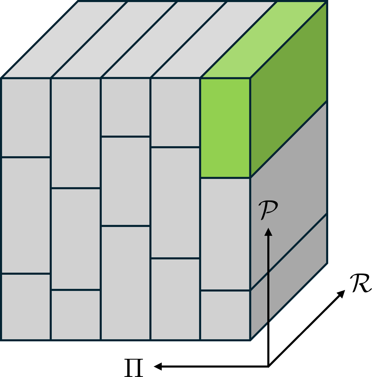
Figure 1: Partitioning for hybrid MDPs

Figure 1 illustrates the partition scheme over $\mathcal{M}\times\Pi=\mathcal{P}\times\mathcal{R}\times\Pi$ described in Assumption 2. Each infoset $\phi$ (represented by the green block in Figure 1) is associated with single policy $\pi_{\phi}$, a subset of transitions, and all reward functions. As shown in Figure 1, the partition over the $\mathcal{P}$ space could be different for different $\pi$.

Appendix C Omitted Details in Section 2

In this section, we show that the algorithms in Xu and Zeevi, (2023) and Liu et al., (2025) are special cases of Algorithm 1.

C.1 Recovering Theorem 3

The decision rule of Liu et al., (2025)’s algorithm corresponds to Eq. (3) with $D^{\pi}(\nu\|\rho)=\mathbb{E}_{M\sim\nu}\mathbb{E}_{o\sim M(\cdot|\pi)}[\text{KL}(\nu_{\boldsymbol{\phi}}(\cdot|\pi,o),\rho)]$. It can be shown that $\textup{Breg}_{D^{\pi}(\cdot\|\rho)}(\nu,\nu^{\prime})=\mathbb{E}_{M\sim\nu}\mathbb{E}_{o\sim M(\cdot|\pi)}\big[\text{KL}(\nu_{\boldsymbol{\phi}}(\cdot|\pi,o),\nu^{\prime}_{\boldsymbol{\phi}}(\cdot|\pi,o))\big]$ in this case. Furthermore, notice that when $\nu=\delta_{M_{t},\pi_{\phi^{\star}}}$, we have $\nu_{\boldsymbol{\phi}}(\cdot|\pi,o)=\delta_{\phi^{\star}}$ according to Definition 2. Thus, the estimation error term in Eq. (6) in Liu et al., (2025)’s algorithm is

$$\mathbb{E}[\textbf{{Est}}] =\mathbb{E}\left[\sum_{t=1}^{T}\left(\text{KL}(\delta_{\phi^{\star}},\rho_{t})-\mathbb{E}_{o\sim M_{t}(\cdot|\pi_{t})}\Big[\text{KL}(\delta_{\phi^{\star}},(\nu_{t})_{\boldsymbol{\phi}}(\cdot|\pi_{t},o))\Big]\right)\right]$$

$$=\mathbb{E}\left[\sum_{t=1}^{T}\left(\text{KL}(\delta_{\phi^{\star}},\rho_{t})-\text{KL}(\delta_{\phi^{\star}},(\nu_{t})_{\boldsymbol{\phi}}(\cdot|\pi_{t},o_{t}))\right)\right]=\mathbb{E}\left[\sum_{t=1}^{T}\log\frac{\nu_{t}(\phi^{\star}|\pi_{t},o_{t})}{\rho_{t}(\phi^{\star})}\right],$$

where in the second equality we use that $o_{t}$ is drawn from $M_{t}(\cdot|\pi_{t})$. Thus, by letting $\rho_{t+1}(\phi)=\nu_{t}(\phi|\pi_{t},o_{t})$, their algorithm achieves $\mathbb{E}[\textbf{{Est}}]=\mathbb{E}\left[\sum_{t=1}^{T}\log\frac{\rho_{t+1}(\phi^{\star})}{\rho_{t}(\phi^{\star})}\right]\leq\log\frac{1}{\rho_{1}(\phi^{\star})}=\log|\Phi|$. Using this in Eq. (6) proves Theorem 3. The results of Xu and Zeevi, (2023) can also be recovered as they are special cases of Liu et al., (2025).

C.2 Recovering results for adversarial MDP with full-information feedback (Liu et al.,, 2025)

For learning with full information feedback in the adversarial MDPs, the learner can observe the full reward function at the end of each episode. In other words, at episode $t$, the reward function $R_{t}:\mathcal{S}\times\mathcal{A}\to[0,1]$ is part of the observation $o_{t}$. In this setting, the $\log|\Pi|$ dependence in the regret bound can be improved to $\log|\mathcal{A}|$. To achieve this, Liu et al., (2025) designed a two-level algorithm and define a new notion called InfoAIR. We can recover this result by instantiating our Algorithm 1 with $\Phi=\{\phi_{P,(a_{s})_{s\in\mathcal{S}}}:~P\in\mathcal{P},a_{s}\in\mathcal{A},\forall s\in\mathcal{S}\}$ where $\phi_{P,(a_{s})_{s\in\mathcal{S}}}=\{((P,R),\pi^{\star}):R\in\mathcal{R},\pi^{\star}=(a_{s})_{s\in\mathcal{S}}\}$, that is, partitioning $\mathcal{M}\times\Pi$ according to the transition kernel and the actions taken by the policy on all states. Then define

$$D^{\pi}(\nu\|\rho)=\mathbb{E}_{(P,R,\pi^{\star})\sim\nu}\mathbb{E}_{o\sim M_{P,R}(\cdot|\pi)}\mathbb{E}_{s\sim d^{\pi,P}}\left[\text{KL}(\nu_{\boldsymbol{a}_{s},\boldsymbol{P}}(\cdot|\pi,o),\rho_{\boldsymbol{a}_{s},\boldsymbol{P}})\right],$$

where $M_{P,R}$ denotes the MDP model with transition kernel $P$ and reward function $R$, and $\rho_{\boldsymbol{a}_{s},\boldsymbol{P}}$ denotes $\rho$’s marginal distribution over $(a_{s},P)$ following our notational convention. Finally, update the posterior as $\rho_{t+1}=\operatorname*{argmin}_{\rho}\sum_{s\in\mathcal{S}}\text{KL}\left(\rho_{\boldsymbol{a}_{s},\boldsymbol{P}},\nu_{\boldsymbol{a}_{s},\boldsymbol{P}}(\cdot|\pi_{t},o_{t})\right)$. This recovers the same regret bound as in Liu et al., (2025) without the need for the two-level design. We also note that the analysis for this result requires our new proof strategy in Eq. (5), as the $D^{\pi}(\nu\|\rho)$ here is not strictly convex in $\nu$ and the previous proof Xu and Zeevi, (2023); Liu et al., (2025) cannot be applied.

Appendix D Concentration Inequality

Lemma 15 (Freedman’s inequality (Beygelzimer et al.,, 2011)).

Let $X_{1},X_{2},\ldots$ be a martingale difference sequence with respect to a filtration $\mathfrak{F}_{1}\subset\mathfrak{F}_{2}\subset\cdots$ such that $\mathbb{E}[X_{t}|\mathfrak{F}_{t}]=0$ and assume $X_{t}\leq B$ almost surely. Then for any $\alpha\geq B$, with probability at least $1-\delta$,

$$\sum_{t=1}^{T}X_{t}\leq\frac{1}{\alpha}\sum_{t=1}^{T}\mathbb{E}[X_{t}^{2}|\mathfrak{F}_{t}]+\alpha\log(1/\delta).$$ (10)

Lemma 16 (Empirical Freedman’s inequality).

Let $X_{1},X_{2},\ldots$ be a sequence with respect to a filtration $\mathfrak{F}_{1}\subset\mathfrak{F}_{2}\subset\cdots$ such that $\mathbb{E}[X_{t}|\mathfrak{F}_{t}]=\mu_{t}$ and assume $\max\{X_{t}-\mu_{t},X_{t}\}\leq B$ almost surely. Then for any $\alpha\geq 4B$, with probability at least $1-\delta$,

$$\sum_{t=1}^{T}(\mu_{t}-X_{t})\leq\frac{4}{\alpha}\sum_{t=1}^{T}X_{t}^{2}+\alpha\log(1/\delta).$$ (11)

Proof.

Denote $\mathbb{E}_{t}[\cdot]=\mathbb{E}[\cdot~|~\mathfrak{F}_{t}]$. We have at any time step

$$\mathbb{E}_{t}\left[\exp\left(\frac{1}{\alpha}(\mu_{t}-X_{t})-\frac{4}{\alpha^{2}}X_{t}^{2}\right)\right]$$

$$\leq\mathbb{E}_{t}\left[1+\frac{1}{\alpha}(\mu_{t}-X_{t})-\frac{4}{\alpha^{2}}X_{t}^{2}+\left(\frac{1}{\alpha}(\mu_{t}-X_{t})-\frac{4}{\alpha^{2}}X_{t}^{2}\right)^{2}\right]$$

$$\leq 1+\mathbb{E}_{t}\left[-\frac{4}{\alpha^{2}}X_{t}^{2}+\frac{2}{\alpha^{2}}((\mu_{t}-X_{t})^{2}+X_{t}^{2})\right]\leq 1.$$

Markov inequality finishes the proof. ∎

Lemma 17.

Let $(X_{1},Y_{1}),(X_{2},Y_{2})\ldots$ be a sequence with respect to a filtration $\mathfrak{F}_{1}\subset\mathfrak{F}_{2}\subset\cdots$ such that $|X_{t}|\leq B$ and $0\leq Y_{t}\leq B$ almost surely. Furthermore, $\mathbb{E}[X_{t}|\mathfrak{F}_{t}]\geq\mathbb{E}[Y_{t}|\mathfrak{F}_{t}]$ and $B\mathbb{E}[X_{t}|\mathfrak{F}_{t}]\geq\mathbb{E}[X_{t}^{2}|\mathfrak{F}_{t}]$. Then with probability at least $1-\delta$,

$$\frac{1}{2}\sum_{t=1}^{T}\mathbb{E}[X_{t}|\mathfrak{F}_{t}]\leq\sum_{t=1}^{T}\left(X_{t}-\frac{1}{4}Y_{t}\right)+9B\log(1/\delta).$$ (12)

Also, with probability at least $1-\delta$,

$$\frac{1}{2}\sum_{t=1}^{T}X_{t}\leq\sum_{t=1}^{T}\left(X_{t}-\frac{1}{4}Y_{t}\right)+9B\log(1/\delta).$$ (13)

Proof.

Denote $\mathbb{E}_{t}[\cdot]=\mathbb{E}[\cdot~|~\mathfrak{F}_{t}]$. Let $c\in[\frac{1}{2},1]$ be a fixed constant, and define $Z_{t}=cX_{t}-\frac{1}{4}Y_{t}$. Applying Lemma 15 with $\alpha=9B$ gives

$$\sum_{t=1}^{T}\left(\mathbb{E}_{t}[Z_{t}]-Z_{t}\right) \leq\frac{1}{9B}\sum_{t=1}^{T}\mathbb{E}_{t}[(\mathbb{E}_{t}[Z_{t}]-Z_{t})^{2}]+9B\log(1/\delta)$$

$$\leq\frac{1}{9B}\sum_{t=1}^{T}\mathbb{E}_{t}[Z_{t}^{2}]+9B\log(1/\delta)$$

$$\leq\frac{1}{9B}\sum_{t=1}^{T}\left(2c^{2}\mathbb{E}_{t}[X_{t}^{2}]+\frac{2}{16}\mathbb{E}_{t}[Y_{t}^{2}]\right)+9B\log(1/\delta)$$

$$\leq\frac{1}{9}\sum_{t=1}^{T}\left(2c^{2}\mathbb{E}_{t}[X_{t}]+\frac{2}{16}\mathbb{E}_{t}[X_{t}]\right)+9\log(1/\delta) \mathbb{E}_{t}[Y_{t}^{2}]\leq B\mathbb{E}_{t}[Y_{t}] Y_{t}\in[0,B]$$ ( because )

Rearranging:

$$\sum_{t=1}^{T}\mathbb{E}_{t}\left[Z_{t}-\left(\frac{2c^{2}}{9}+\frac{1}{72}\right)X_{t}\right]\leq\sum_{t=1}^{T}Z_{t}+9B\log(1/\delta).$$ (14)

To prove Eq. (12), let $c=1$, which gives $\mathbb{E}_{t}\left[Z_{t}-\left(\frac{2c^{2}}{9}+\frac{1}{72}\right)X_{t}\right]=\mathbb{E}_{t}\left[X_{t}-\frac{1}{4}Y_{t}-\frac{17}{72}X_{t}\right]\geq\frac{1}{2}\mathbb{E}_{t}[X_{t}]$. Combining this with Eq. (14) proves Eq. (12). To prove Eq. (13), let $c=\frac{1}{2}$. which gives $\mathbb{E}_{t}\left[Z_{t}-\left(\frac{2c^{2}}{9}+\frac{1}{72}\right)X_{t}\right]=\mathbb{E}_{t}\left[\frac{1}{2}X_{t}-\frac{1}{4}Y_{t}-\frac{5}{72}X_{t}\right]\geq 0$. Combining this with Eq. (14) and rearranging proves Eq. (13). ∎

Appendix E Mirror Descent

Lemma 18 (First-order optimality condition).

For any concave and differentiable function $F$, if $\nu^{\prime}\in\operatorname*{argmax}_{\nu\in\Omega}F(\nu)$ for some convex set $\Omega$, then $F(\nu)\leq F(\nu^{\prime})-\textup{Breg}_{(-F)}(\nu,\nu^{\prime})$ for any $\nu\in\Omega$.

Proof.

Define $G=-F$. Then $G$ is convex and $\nu^{\prime}\in\operatorname*{argmin}_{\nu^{\prime}}G(\nu^{\prime})$. We have by the definition of Bregman divergence $\textup{Breg}_{G}(\nu,\nu^{\prime})=G(\nu)-G(\nu^{\prime})-\langle\nabla G(\nu^{\prime}),\nu-\nu^{\prime}\rangle$, and first-order optimality condition $\langle\nabla G(\nu^{\prime}),\nu-\nu^{\prime}\rangle\geq 0$. Thus, $G(\nu)\geq G(\nu^{\prime})+\textup{Breg}_{G}(\nu,\nu^{\prime})$, which is equivalent to $F(\nu)\leq F(\nu^{\prime})+\textup{Breg}_{(-F)}(\nu,\nu^{\prime})$. ∎

Lemma 19.

Let $g:\Phi\to[-1,1]$ be any function and let $\nu,\rho\in\Delta(\Phi)$. Then for any $\eta>0$,

$$\mathbb{E}_{\phi\sim\nu}[g(\phi)]-\mathbb{E}_{\phi\sim\rho}[g(\phi)]-\frac{1}{\eta}\text{KL}(\nu,\rho)\leq\eta.$$

Proof.

$$\mathbb{E}_{\phi\sim\nu}[g(\phi)]-\mathbb{E}_{\phi\sim\rho}[g(\phi)]\leq 2D_{\text{TV}}(\nu,\rho)\leq 2\sqrt{\text{KL}(\nu,\rho)}\leq\frac{1}{\eta}\text{KL}(\nu,\rho)+\eta,$$

where we use Pinsker’s inequality and AM-GM inequality. ∎

Lemma 20 (Mirror descent with auxiliary terms).

Let $F_{t}$ be a convex function over $\Delta_{N}$, and let $\ell_{t},b_{t}\in\mathbb{R}^{N}$ with $\ell_{t}^{2}$ denoting $(\ell_{t}(1)^{2},\ldots,\ell_{t}(N)^{2})$. Then the update $p_{1}=\frac{1}{N}\mathbf{1}$ and

$$p_{t+1}=\operatorname*{argmin}_{p\in\Delta_{N}}\Big\{\left\langle p,\ell_{t}+4\gamma\ell_{t}^{2}+b_{t}\right\rangle+F_{t}(p)+\frac{1}{\gamma}\text{KL}(p,p_{t})\Big\}$$

with $\gamma|\ell_{t}(i)|\leq\frac{1}{16}$ and $0\leq\gamma b_{t}(i)\leq\frac{1}{4}$ for all $i\in[N]$ ensures for any $p^{\star}\in\Delta_{N}$,

$$\sum_{t=1}^{T}\left\langle p_{t},\ell_{t}\right\rangle$$

$$\leq\frac{\log N}{\gamma}+\sum_{t=1}^{T}\Big(\left\langle p^{\star},\ell_{t}+4\gamma\ell_{t}^{2}\right\rangle+\left\langle p^{\star},b_{t}\right\rangle-\frac{1}{2}\left\langle p_{t},b_{t}\right\rangle+F_{t}(p^{\star})-F_{t}(p_{t+1})-\textup{Breg}_{F_{t}}(p^{\star},p_{t+1})\Big).$$

Proof.

By Lemma 18,

$$\left\langle p_{t+1},\ell_{t}+4\gamma\ell_{t}^{2}+b_{t}\right\rangle+F_{t}(p_{t+1})+\frac{1}{\gamma}\text{KL}(p_{t+1},p_{t})$$

$$\leq\left\langle p^{\star},\ell_{t}+4\gamma\ell_{t}^{2}+b_{t}\right\rangle+F_{t}(p^{\star})+\frac{1}{\gamma}\text{KL}(p^{\star},p_{t})-\textup{Breg}_{F_{t}}(p^{\star},p_{t+1})-\frac{1}{\gamma}\text{KL}(p^{\star},p_{t+1}).$$

Rearranging gives

$$\left\langle p_{t},\ell_{t}+4\gamma\ell_{t}^{2}\right\rangle$$

$$\leq\left\langle p^{\star},\ell_{t}+4\gamma\ell_{t}^{2}\right\rangle+\left\langle p_{t}-p_{t+1},\ell_{t}+4\gamma\ell_{t}^{2}+b_{t}\right\rangle-\frac{1}{\gamma}\text{KL}(p_{t+1},p_{t})$$

$$\quad+\left\langle p^{\star}-p_{t},b_{t}\right\rangle+\frac{\text{KL}(p^{\star},p_{t})-\text{KL}(p^{\star},p_{t+1})}{\gamma}+F_{t}(p^{\star})-F_{t}(p_{t+1})-\textup{Breg}_{F_{t}}(p^{\star},p_{t+1}).$$ (15)

Since $\gamma|\ell_{t}(i)+4\gamma\ell_{t}(i)^{2}+b_{t}(i)|\leq\frac{1}{16}+4\times(\frac{1}{16})^{2}+\frac{1}{4}\leq 1$, by Lemma 19 we have

$$\left\langle p_{t}-p_{t+1},\ell_{t}+4\gamma\ell_{t}^{2}+b_{t}\right\rangle-\frac{1}{\gamma}\text{KL}(p_{t+1},p_{t})$$

$$\leq\gamma\left\langle p_{t},(\ell_{t}+4\gamma\ell_{t}^{2}+b_{t})^{2}\right\rangle$$

$$\leq 2\gamma\left\langle p_{t},({\textstyle\frac{5}{4}}\ell_{t})^{2}\right\rangle+2\gamma\left\langle p_{t},b_{t}^{2}\right\rangle$$

$$\leq\left\langle p_{t},4\gamma\ell_{t}^{2}\right\rangle+\frac{1}{2}\left\langle p_{t},b_{t}\right\rangle.$$

Using this in Eq. (15) we get

$$\left\langle p_{t},\ell_{t}\right\rangle \leq\left\langle p^{\star},\ell_{t}+4\gamma\ell_{t}^{2}\right\rangle+\left\langle p^{\star},b_{t}\right\rangle-\frac{1}{2}\left\langle p_{t},b_{t}\right\rangle$$

$$\qquad+\frac{\text{KL}(p^{\star},p_{t})-\text{KL}(p^{\star},p_{t+1})}{\gamma}+F_{t}(p^{\star})-F_{t}(p_{t+1})-\textup{Breg}_{F_{t}}(p^{\star},p_{t+1}).$$

Summing over $t$ gives the desired inequality. ∎

Appendix F Estimation Procedures

We present the choices of PosteriorUpdate as standalone online learning algorithms because they might be of independent interest.

F.1 Average estimation error minimization via batching

1Input: An estimation function $\ell_{h}:\Phi\times\mathcal{O}\to[-B,B]^{N}$ satisfying Assumption 5.

2 Parameter: $\tau=T^{\frac{1}{3}},\beta=7\tau N\iota$, $\gamma=\frac{1}{2\beta}$, $\iota=\log(12NKH/\delta)$.

3 for $k=1,2,\ldots,K$ do

4    Receive observations $o_{t}\sim M_{t}(\cdot|\pi_{k})$ for all $t\in\mathcal{I}_{k}=\{(k-1)\tau+1,\ldots,k\tau\}$.

5    Split $\mathcal{I}_{k}$ into two sub-intervals of equal size:

$$\mathcal{I}_{k}^{-}=\{(k-1)\tau+1,\ldots,(k-1)\tau+\tfrac{\tau}{2}\}\quad\text{and}\quad\mathcal{I}_{k}^{+}=\{(k-1)\tau+\tfrac{\tau}{2}+1,\ldots,k\tau\}.$$

Define for all $j\in[N]$,

$$L_{k}(\phi)_{j} =\frac{\tau}{B^{2}H}\sum_{h=1}^{H}\left(\frac{1}{|\mathcal{I}_{k}^{-}|}\sum_{t\in\mathcal{I}_{k}^{-}}\ell_{h}(\phi;o_{t,h})_{j}\right)\left(\frac{1}{|\mathcal{I}_{k}^{+}|}\sum_{t\in\mathcal{I}_{k}^{+}}\ell_{h}(\phi;o_{t,h})_{j}\right)\,,\quad L_{k}(\phi)=\sum_{j=1}^{N}L_{k}(\phi)_{j}.$$

6   Let $(F_{t})_{t\in\mathcal{I}_{k}}:\Delta(\Phi)\to\mathbb{R}$ be convex functions. Calculate

$$\rho_{k+1}=\operatorname*{argmin}_{\rho\in\Delta(\Phi)}\left\{\left\langle\rho,L_{k}+(4\gamma+2\beta^{-1})L_{k}^{2}\right\rangle+\sum_{t\in\mathcal{I}_{k}}F_{t}(\rho)+\frac{1}{\gamma}\text{KL}(\rho,\rho_{k})\right\}.$$ (16)

Algorithm 2 Epoch-based learning algorithm for average estimation error

Lemma 21.

With probability at least $1-\delta/3$, Algorithm 2 satisfies

$$\frac{1}{B^{2}H}\sum_{k=1}^{K}\sum_{\phi}\rho_{k}(\phi)\sum_{t\in\mathcal{I}_{k}}\max_{j\in[N]}\sum_{h=1}^{H}\left(\mathbb{E}^{\pi_{k},M_{t}}[\ell_{h}(\phi;o_{h})_{j}]\right)^{2}\leq\sum_{k=1}^{K}\sum_{\phi}\rho_{k}(\phi)\left(L_{k}(\phi)+\frac{1}{\beta}L_{k}(\phi)^{2}\right)+4\beta\log(3/\delta)\,.$$

Proof.

By Assumption 5, for any $t,t^{\prime}\in\mathcal{I}_{k}$ it holds that

$$\mathbb{E}^{\pi_{k},M_{t}}\left[\ell_{h}(\phi;o_{h})\right]=\mathbb{E}^{\pi_{k},M_{t^{\prime}}}\left[\ell_{h}(\phi;o_{h})\right].$$

We denote $\bar{\ell}_{k,h}(\phi)=\mathbb{E}^{\pi_{k},M_{t}}[\ell_{h}(\phi;o_{h})]$ for any $t\in\mathcal{I}_{k}$.

Clearly, the left-hand side of the desired inequality is upper bounded by

$$\frac{1}{B^{2}H}\sum_{k=1}^{K}\sum_{\phi}\rho_{k}(\phi)\sum_{t\in\mathcal{I}_{k}}\sum_{j=1}^{N}\sum_{h=1}^{H}\left(\mathbb{E}^{\pi_{k},M_{t}}[\ell_{h}(\phi;o_{h})_{j}]\right)^{2}=\frac{\tau}{B^{2}H}\sum_{k=1}^{K}\sum_{\phi}\rho_{k}(\phi)\sum_{j=1}^{N}\sum_{h=1}^{H}\bar{\ell}_{k,h}(\phi)^{2}_{j}$$

By construction, $\mathbb{E}_{k}[L_{k}(\phi)]=\frac{\tau}{B^{2}H}\sum_{j=1}^{N}\sum_{h=1}^{H}\bar{\ell}_{k,h}(\phi)^{2}_{j}$ due to the conditional independence of the observations. Furthermore, we have $L_{k}(\phi)\in[-\tau N,\tau N]$. Therefore, we can use Lemma 16 on the sequence $X_{k}=-\sum_{\phi}\rho_{k}(\phi)L_{k}(\phi)$ with $\beta\geq 7\tau N$:

$$\frac{\tau}{B^{2}H}\sum_{k=1}^{K}\sum_{\phi}\rho_{k}(\phi)\sum_{j=1}^{N}\sum_{h=1}^{H}\bar{\ell}_{k,h}(\phi)^{2}_{j}\leq\sum_{k=1}^{K}\sum_{\phi}\rho_{k}(\phi)\left(L_{k}(\phi)+\frac{1}{\beta}L_{k}(\phi)^{2}\right)+4\beta\log(3/\delta)\,.$$

∎

Lemma 22.

With probability at least $1-\delta/3$,

$$\sum_{k=1}^{K}L_{k}(\phi^{\star})^{2}\leq KN^{2}\log^{2}(12NKH/\delta).$$

Proof.

By Assumption 5 and Lemma 15, for any $j,k,h$, we have with probability $1-\delta$,

$$\left|\sum_{t\in\mathcal{I}_{k}^{-}}\ell_{h}(\phi^{\star},o_{t,h})_{j}\right|=\left|\sum_{t\in\mathcal{I}_{k}^{-}}\ell_{h}(\phi^{\star},o_{t,h})_{j}-\sum_{t\in\mathcal{I}_{k}^{-}}\mathbb{E}^{\pi_{k},M_{t}}[\ell_{h}(\phi^{\star};o_{h})]\right|\leq B\sqrt{\tau\log(12/\delta)}$$

$$\left|\sum_{t\in\mathcal{I}_{k}^{+}}\ell_{h}(\phi^{\star},o_{t,h})_{j}\right|=\left|\sum_{t\in\mathcal{I}_{k}^{+}}\ell_{h}(\phi^{\star},o_{t,h})_{j}-\sum_{t\in\mathcal{I}_{k}^{+}}\mathbb{E}^{\pi_{k},M_{t}}[\ell_{h}(\phi^{\star};o_{h})]\right|\leq B\sqrt{\tau\log(12/\delta)}\,.$$

Via a union bound over all these events, this holds simultaneously for all $j,k,h$. Hence with probability $1-\delta$, we have $|L_{k}(\phi^{\star})_{j}|\leq\frac{\tau}{B^{2}H}H\left(\frac{1}{\tau}B\sqrt{\tau\log(12NKH/\delta)}\right)^{2}=\log(12NKH/\delta)$ for all $j,k$ simultaneously. Summing over $j$ and $k$ finishes the proof. ∎

Lemma 23.

With probability at least $1-\delta/3$, we have

$$\sum_{k=1}^{K}L_{k}(\phi^{\star})\leq\frac{1}{\beta}\sum_{k=1}^{K}L_{k}(\phi^{\star})^{2}+4\beta\log(6/\delta)$$

Proof.

Define the random variable $X_{k}=\min\{L_{k}(\phi^{\star}),N\log(12NKH/\delta)\}$. By Lemma 16 we have with probability at least $1-\delta/6$,

$$\sum_{k=1}^{K}X_{t}\leq\frac{1}{\beta}\sum_{k=1}^{K}L_{k}(\phi^{\star})^{2}+4\beta\log(6/\delta)\,,$$

where we use that $\mathbb{E}_{k}[X_{k}]\leq\mathbb{E}_{k}[L_{k}(\phi^{\star})]=0$. Finally note that with probability $1-\delta/6$ we have $L_{k}(\phi^{\star})=X_{k}$ for all $k$ by the proof of Lemma 22. Combining both events finishes the proof. ∎

Lemma 24.

With probability at least $1-\delta$, Algorithm 2 satisfies

$$\frac{1}{B^{2}H}\sum_{k=1}^{K}\sum_{\phi}\rho_{k}(\phi)\sum_{t\in\mathcal{I}_{k}}\max_{j\in[N]}\sum_{h=1}^{H}\left(\mathbb{E}^{\pi_{k},M_{t}}\left[\ell_{h}(\phi;o_{h})_{j}\right]\right)^{2}\leq O\left(NT^{\frac{1}{3}}\log|\Phi|\right)$$

$$\quad+\sum_{k=1}^{K}\sum_{t\in\mathcal{I}_{k}}(F_{t}(\delta_{\phi^{\star}})-F_{t}(\rho_{k+1})-\textup{Breg}_{F_{t}}(\delta_{\phi^{\star}},\rho_{k+1})).$$

Proof of Lemma 24.

By union bound, the events of Lemma 21, Lemma 22, and Lemma 23 hold simultaneously with probability $1-\delta$. Observe that the update of $\rho_{k}$ (Eq. (16)) is in the form specified in Lemma 20. Invoking Lemma 20 with $b_{k}=\frac{2}{\beta}L_{k}^{2}$, we get

$$\sum_{k=1}^{K}\left\langle\rho_{k},L_{k}+\frac{1}{\beta}L_{k}^{2}\right\rangle\leq\frac{\log|\Phi|}{\gamma}$$ (17)

$$\quad+\sum_{k=1}^{K}\left(L_{k}(\phi^{\star})+\left(4\gamma+\frac{2}{\beta}\right)L_{k}(\phi^{\star})^{2}+\sum_{t\in\mathcal{I}_{k}}(F_{t}(\delta_{\phi^{\star}})-F_{t}(\rho_{k+1})-\textup{Breg}_{F_{t}}(\delta_{\phi^{\star}},\rho_{k+1}))\right).$$

Chaining Lemma 22 and Lemma 23,

$$\sum_{k=1}^{K}\left(L_{k}(\phi^{\star})+\left(4\gamma+\frac{2}{\beta}\right)L_{k}(\phi^{\star})^{2}\right)$$

$$\leq 4\beta\log(6/\delta)+\left(4\gamma+\frac{3}{\beta}\right)KN^{2}\log^{2}(12NKH/\delta).$$

Using Lemma 21 and substituting $\beta=7\tau N\iota$, $\gamma=\frac{1}{2\beta}$ yields

$$\frac{1}{B^{2}H}\sum_{k=1}^{K}\sum_{\phi}\rho_{k}(\phi)\sum_{t\in\mathcal{I}_{k}}\max_{j\in[N]}\sum_{h=1}^{H}\left(\mathbb{E}^{\pi_{k},M_{t}}[\ell_{h}(\phi;o_{h})_{j}]\right)^{2}\leq 35\tau N\iota+20\frac{KN\iota}{\tau}$$

Using $K=T/\tau$ and tuning $\tau=T^{\frac{1}{3}}$ yields $O(T^{\frac{1}{3}}N\iota)$. ∎

F.2 Squared estimation error minimization via bi-level learning

1Input: An estimation function $\xi_{h}:\Phi\times\Phi\times\mathcal{O}\to[0,B^{2}]$ satisfying Assumption 6.

2 Parameter: $\iota=64\log|\Phi|$, $\gamma=\frac{1}{4\iota}$.

3 $\rho_{1}(\phi)=1/|\Phi|,\,\forall\phi\in\Phi$ and $q_{1}(\phi^{\prime}|\phi)=1/|\Phi|$, $\forall\phi^{\prime},\phi\in\Phi$.

4 for $t=1,2,\ldots,T$ do

5    Receive observation $o_{t}\sim M_{t}(\cdot|\pi_{t})$.

6    Define

$$\Delta_{t}(\phi^{\prime},\phi) =\frac{1}{B^{2}H}\sum_{h=1}^{H}\xi_{h}(\phi^{\prime},\phi,o_{t,h}),$$

$$L_{t}(\phi) =\Delta_{t}(\phi,\phi)-\mathbb{E}_{\phi^{\prime}\sim q_{t}(\cdot|\phi)}\left[\Delta_{t}(\phi^{\prime},\phi)\right],$$

$$b_{t}(\phi) =\frac{[\rho_{t}(\phi)-\max_{s<t}\rho_{s}(\phi)]_{+}}{\rho_{t}(\phi)}\iota.$$

Let $F_{t}:\Delta(\Phi)\to\mathbb{R}$ be a convex function. Calculate

$$\rho_{t+1}=\operatorname*{argmin}_{\rho\in\Delta(\Phi)}\left\{\left\langle\rho,L_{t}+4\gamma L_{t}^{2}+b_{t}\right\rangle+F_{t}(\rho)+\frac{1}{\gamma}\text{KL}(\rho,\rho_{t})\right\},$$ (18)

$$q_{t+1}(\phi^{\prime}|\phi)\propto\exp\left(-\alpha_{t}(\phi)\sum_{s=1}^{t}\rho_{s}(\phi)\Delta_{s}(\phi^{\prime},\phi)\right)\quad\text{where \ \ }\alpha_{t}(\phi)=\frac{1}{16\max_{s\leq t}\rho_{s}(\phi)}.$$

Algorithm 3 Bi-level learning algorithm for squared estimation error

Lemma 25.

With probability at least $1-\delta$,

$$\sum_{t=1}^{T}\left\langle\rho_{t},L_{t}\right\rangle\leq\frac{\log|\Phi|}{\gamma}$$

$$\quad+\sum_{t=1}^{T}\left(-\frac{1}{2}\left\langle\rho_{t},b_{t}\right\rangle+b_{t}(\phi^{\star})+F_{t}(\delta_{\phi^{\star}})-F_{t}(\rho_{t+1})-\textup{Breg}_{F_{t}}(\delta_{\phi^{\star}},\rho_{t+1})\right)+O\left(\log(1/\delta)\right).$$

Proof of Lemma 25.

Observe that the update of $\rho_{t}$ (Eq. (18)) is in the form specified in Lemma 20. Invoking Lemma 20, we get

$$\sum_{t=1}^{T}\left\langle\rho_{t},L_{t}\right\rangle\leq\frac{\log|\Phi|}{\gamma}$$ (19)

$$\quad+\sum_{t=1}^{T}\left(L_{t}(\phi^{\star})+4\gamma L_{t}(\phi^{\star})^{2}+b_{t}(\phi^{\star})-\frac{1}{2}\left\langle\rho_{t},b_{t}\right\rangle+F_{t}(\delta_{\phi^{\star}})-F_{t}(\rho_{t+1})-\textup{Breg}_{F_{t}}(\delta_{\phi^{\star}},\rho_{t+1})\right).$$

By Assumption 6 we have

$$0\leq\mathbb{E}_{t}[L_{t}(\phi^{\star})^{2}] =\mathbb{E}_{t}\left[\left(\Delta_{t}(\phi^{\star},\phi^{\star})-\mathbb{E}_{\phi^{\prime}\sim q_{t}(\cdot|\phi^{\star})}\left[\Delta_{t}(\phi^{\prime},\phi^{\star})\right]\right)^{2}\right]$$

$$\leq\mathbb{E}_{\phi^{\prime}\sim q_{t}(\cdot|\phi^{\star})}\left[\mathbb{E}_{t}\left[\left(\Delta_{t}(\phi^{\star},\phi^{\star})-\Delta_{t}(\phi^{\prime},\phi^{\star})\right)^{2}\right]\right]$$ (Jensen’s inequality)

$$\leq\mathbb{E}_{\phi^{\prime}\sim q_{t}(\cdot|\phi^{\star})}\left[\mathbb{E}_{t}\left[\left(\Delta_{t}(\mathcal{T}_{M_{t}}\phi^{\star},\phi^{\star})-\Delta_{t}(\phi^{\prime},\phi^{\star})\right)^{2}\right]\right] M_{t}\in\phi^{\star} \mathcal{T}_{M_{t}}\phi^{\star}=\phi^{\star}$$ ( and thus )

$$\leq 4\mathbb{E}_{\phi^{\prime}\sim q_{t}(\cdot|\phi^{\star})}\left[\mathbb{E}_{t}\left[\Delta_{t}(\phi^{\prime},\phi^{\star})-\Delta_{t}(\mathcal{T}_{M_{t}}\phi^{\star},\phi^{\star})\right]\right]$$ (by Assumption 6)

$$=4\mathbb{E}_{\phi^{\prime}\sim q_{t}(\cdot|\phi^{\star})}\left[\mathbb{E}_{t}\left[\Delta_{t}(\phi^{\prime},\phi^{\star})-\Delta_{t}(\phi^{\star},\phi^{\star})\right]\right]$$

$$=-4\mathbb{E}_{t}[L_{t}(\phi^{\star})].$$

This allows us to apply Lemma 17 with $X_{t}=-L_{t}(\phi^{\star})$ and $Y_{t}=\frac{1}{4}X_{t}^{2}$, which gives

$$\sum_{t=1}^{T}\left(L_{t}(\phi^{\star})+4\gamma L_{t}(\phi^{\star})^{2}\right) \leq\sum_{t=1}^{T}\left(L_{t}(\phi^{\star})+\frac{1}{16}L_{t}(\phi^{\star})^{2}\right)$$

$$\leq\frac{1}{2}\sum_{t=1}^{T}\mathbb{E}_{t}[L_{t}(\phi^{\star})]+36\log(1/\delta)\leq 36\log(1/\delta).$$

Combining this with Eq. (19) finishes the proof. ∎

Lemma 26.

With probability at least $1-\delta$,

$$\sum_{t=1}^{T}\mathbb{E}_{\phi\sim\rho_{t}}\mathbb{E}_{\phi^{\prime}\sim q_{t}(\cdot|\phi)}[\Delta_{t}(\phi^{\prime},\phi)-\Delta_{t}(\mathcal{T}_{M_{t}}\phi,\phi)]\leq 32\sum_{\phi}\max_{t\leq T}\rho_{t}(\phi)\log|\Phi|+72\log(1/\delta).$$

Proof.

By Assumption 6, we have $\mathcal{T}_{M_{t}}\phi=\mathcal{T}_{M_{t^{\prime}}}\phi$ for all $\phi$ and all $t,t^{\prime}\in[T]$. We denote $\mathcal{T}\phi=\mathcal{T}_{M_{t}}\phi$ for any $t$. By the exponential weight update, for any $\phi$,

$$\sum_{t=1}^{T}\sum_{\phi^{\prime}}q_{t}(\phi^{\prime}|\phi)\rho_{t}(\phi)\left(\Delta_{t}(\phi^{\prime},\phi)-\Delta_{t}(\mathcal{T}_{M_{t}}\phi,\phi)\right)$$

$$=\sum_{t=1}^{T}\sum_{\phi^{\prime}}q_{t}(\phi^{\prime}|\phi)\rho_{t}(\phi)\left(\Delta_{t}(\phi^{\prime},\phi)-\Delta_{t}(\mathcal{T}\phi,\phi)\right)$$

$$\leq\frac{\log|\Phi|}{\alpha_{T}(\phi)}+\sum_{t=1}^{T}\sum_{\phi^{\prime}}\alpha_{t}(\phi)q_{t}(\phi^{\prime}|\phi)\rho_{t}(\phi)^{2}\left(\Delta_{t}(\phi^{\prime},\phi)-\Delta_{t}(\mathcal{T}\phi,\phi)\right)^{2}$$

$$\leq 16\max_{t\leq T}\rho_{t}(\phi)\log|\Phi|+\frac{1}{16}\sum_{t=1}^{T}\sum_{\phi^{\prime}}q_{t}(\phi^{\prime}|\phi)\rho_{t}(\phi)\left(\Delta_{t}(\phi^{\prime},\phi)-\Delta_{t}(\mathcal{T}\phi,\phi)\right)^{2}.$$

Rearranging and summing over $\phi$:

$$\sum_{t=1}^{T}\mathbb{E}_{\phi\sim\rho_{t}}\mathbb{E}_{\phi^{\prime}\sim q_{t}(\cdot|\phi)}\left[\Delta_{t}(\phi^{\prime},\phi)-\Delta_{t}(\mathcal{T}\phi,\phi)-\frac{1}{16}(\Delta_{t}(\phi^{\prime},\phi)-\Delta_{t}(\mathcal{T}\phi,\phi))^{2}\right]$$

$$\qquad\qquad\leq 16\sum_{\phi}\max_{t\leq T}\rho_{t}(\phi)\log|\Phi|.$$ (20)

Define

$$X_{t} =\mathbb{E}_{\phi\sim\rho_{t}}\mathbb{E}_{\phi^{\prime}\sim q_{t}(\cdot|\phi)}\left[\Delta_{t}(\phi^{\prime},\phi)-\Delta_{t}(\mathcal{T}\phi,\phi)\right],$$

$$Y_{t} =\frac{1}{4}\mathbb{E}_{\phi\sim\rho_{t}}\mathbb{E}_{\phi^{\prime}\sim q_{t}(\cdot|\phi)}\left[\left(\Delta_{t}(\phi^{\prime},\phi)-\Delta_{t}(\mathcal{T}\phi,\phi)\right)^{2}\right].$$

By Assumption 6 we have $\mathbb{E}_{t}[Y_{t}]\leq\mathbb{E}_{t}[X_{t}]$. By Jensen’s inequality, $\mathbb{E}_{t}[X_{t}^{2}]\leq 4B^{2}H\mathbb{E}_{t}[Y_{t}]\leq 4B^{2}H\mathbb{E}_{t}[X_{t}]$. Invoking Lemma 17 and using Eq. (20) give

$$\frac{1}{2}\sum_{t=1}^{T}X_{t} \leq\sum_{t=1}^{T}\left(X_{t}-\frac{1}{4}Y_{t}\right)+36\log(1/\delta)\leq 16\sum_{\phi}\max_{t\leq T}\rho_{t}(\phi)\log|\Phi|+36\log(1/\delta),$$

proving the desired inequality.

∎

Lemma 27.

With probability at least $1-\delta$,

$$\sum_{t=1}^{T}\mathbb{E}_{\phi\sim\rho_{t}}\left[\Delta_{t}(\phi,\phi)-\Delta_{t}(\mathcal{T}_{M_{t}}\phi,\phi)\right]$$

$$\leq\sum_{t=1}^{T}\left(F_{t}(\delta_{\phi^{\star}})-F_{t}(\rho_{t+1})-\textup{Breg}_{F_{t}}(\delta_{\phi^{\star}},\rho_{t+1})\right)+O\left(\log^{2}(|\Phi|/\delta)\right).$$

Proof.

By Assumption 6, we have $\mathcal{T}_{M_{t}}\phi=\mathcal{T}_{M_{t^{\prime}}}\phi$ for all $\phi$ and all $t,t^{\prime}\in[T]$. We denote $\mathcal{T}\phi=\mathcal{T}_{M_{t}}\phi$ for any $t$.

$$\mathbb{E}_{\phi\sim\rho_{t}}[L_{t}(\phi)] =\mathbb{E}_{\phi\sim\rho_{t}}[\Delta_{t}(\phi,\phi)-\mathbb{E}_{\phi^{\prime}\sim q_{t}(\cdot|\phi)}[\Delta_{t}(\phi^{\prime},\phi)]]$$

$$=\mathbb{E}_{\phi\sim\rho_{t}}\left[\Delta_{t}(\phi,\phi)-\Delta_{t}(\mathcal{T}\phi,\phi)-\left(\mathbb{E}_{\phi^{\prime}\sim q_{t}(\cdot|\phi)}[\Delta_{t}(\phi^{\prime},\phi)]-\Delta_{t}(\mathcal{T}\phi,\phi)\right)\right].$$

Combining this with Lemma 25, we get

$$\sum_{t=1}^{T}\mathbb{E}_{\phi\sim\rho_{t}}\left[\Delta_{t}(\phi,\phi)-\Delta_{t}(\mathcal{T}\phi,\phi)\right]$$

$$\leq\frac{\log|\Phi|}{\gamma}+\sum_{t=1}^{T}\left(-\frac{1}{2}\left\langle\rho_{t},b_{t}\right\rangle+b_{t}(\phi^{\star})+F_{t}(\delta_{\phi^{\star}})-F_{t}(\rho_{t+1})-\textup{Breg}_{F_{t}}(\delta_{\phi^{\star}},\rho_{t+1})\right)$$

$$\qquad+O\left(\log(1/\delta)\right)+\sum_{t=1}^{T}\mathbb{E}_{\phi\sim\rho_{t}}\mathbb{E}_{\phi^{\prime}\sim q_{t}(\cdot|\phi)}\left[\Delta_{t}(\phi^{\prime},\phi)-\Delta_{t}(\mathcal{T}\phi,\phi)\right]$$

$$\leq\sum_{t=1}^{T}\left(-\frac{1}{2}\left\langle\rho_{t},b_{t}\right\rangle+b_{t}(\phi^{\star})+F_{t}(\delta_{\phi^{\star}})-F_{t}(\rho_{t+1})-\textup{Breg}_{F_{t}}(\delta_{\phi^{\star}},\rho_{t+1})\right)$$

$$\qquad+O\left(\log^{2}(|\Phi|/\delta)\right)+32\sum_{\phi}\max_{t\leq T}\rho_{t}(\phi)\log|\Phi|. \gamma$$ (by Lemma 26 and the value of )

Note that

$$32\log|\Phi|\sum_{\phi}\max_{t\leq T}\rho_{t}(\phi) =32\log|\Phi|\sum_{\phi}\left(\rho_{1}(\phi)+\sum_{t=2}^{T}[\rho_{t}(\phi)-\max_{s<t}\rho_{s}(\phi)]_{+}\right)$$

$$=32\log|\Phi|\sum_{\phi}\left(\rho_{1}(\phi)+\sum_{t=2}^{T}\rho_{t}(\phi)\frac{[\rho_{t}(\phi)-\max_{s<t}\rho_{s}(\phi)]_{+}}{\rho_{t}(\phi)}\right)$$

$$=\frac{1}{2}\sum_{t=1}^{T}\left\langle\rho_{t},b_{t}\right\rangle$$

and

$$\sum_{t=1}^{T}b_{t}(\phi^{\star}) =O(\log|\Phi|)\times\sum_{t=1}^{T}\frac{\max_{s\leq t}\rho_{s}(\phi^{\star})-\max_{s\leq t-1}\rho_{s}(\phi^{\star})}{\max_{s\leq t}\rho_{s}(\phi^{\star})}$$

$$\leq O(\log|\Phi|)\times\left(1+\sum_{t=2}^{T}\ln\frac{\max_{s\leq t}\rho_{s}(\phi^{\star})}{\max_{s\leq t-1}\rho_{s}(\phi^{\star})}\right) 1-x\leq\ln\frac{1}{x}$$ ()

$$\leq O\left(\log^{2}|\Phi|\right).$$

Combining inequalities above proves the lemma.

∎

Appendix G Omitted Details in Section 4

We define a batched version of Algorithm 1 in Algorithm 4. When the batch size $\tau=1$, it is exactly Algorithm 1. One can also think of Algorithm 4 as a special case of Algorithm 1 where PosteriorUpdate makes a real update only when $t=k\tau$ for $k=1,2,\ldots$, and keeps $\rho_{t+1}=\rho_{t}$ otherwise.

1Input: Partition set $\Phi$ and its union $\Psi$ (defined in Section 2.1). Batch size $\tau$.

2 $\rho_{1}(\phi)=1/|\Phi|,\,\forall\phi\in\Phi$.

3 for $k=1,2,\ldots,K$ do

4    Set $p_{k},\nu_{k}$ as the solution of the following minimax optimization (defined in Eq. (2)):

$$\min_{p\in\Delta(\Pi)}\max_{\nu\in\Delta(\Psi)}\mathsf{AIR}^{\Phi,D}_{\eta}(p,\nu;\rho_{k}).$$ (21)

Execute $\pi_{k}$ in rounds $t\in\{(k-1)\tau+1,\ldots,k\tau\}=\mathcal{I}_{k}$ and receive observations $(o_{t})_{t\in\mathcal{I}_{k}}$.

5   -5pt

$$\text{Update\ }\rho_{k+1}=\textsc{PosteriorUpdate}(\nu_{k},\rho_{k},\pi_{k},(o_{t})_{t\in\mathcal{I}_{k}}).$$ (22)

6

-3pt

Algorithm 4 General Batched Framework

G.1 Assumption reductions

Proof of Lemma 8.

In the stochastic setting, by Assumption 1 we have $f_{\phi}(s,a)=Q^{\star}(s,a;M)$ and $f_{\phi}(s)=V^{\star}(s;M)$ for any $M\in\phi$. Hence

$$\mathbb{E}^{\pi,M}[\ell_{h}(\phi;o_{h})] =\mathbb{E}^{\pi,M}[f_{\phi}(s_{h},a_{h})-r_{h}-f_{\phi}(s_{h+1})]$$

$$=\mathbb{E}^{\pi,M}[Q^{\star}(s_{h},a_{h};M)-r_{h}-V^{\star}(s_{h+1};M)]=0.$$

In the hybrid setting, we have by Assumption 2 and Assumption 3 that $f_{\phi}(s,a;R)=Q^{\pi_{\phi}}(s,a;(P,R))$ and $f_{\phi}(s;R)=V^{\pi_{\phi}}(s;(P,R))$ for any $P\in\phi$. Hence, for any $j\in[d]$, defining $R^{\prime}$ such that $R^{\prime}(s,a)=\varphi(s,a)_{j}$, we have for $(P,R)\in\phi$,

$$\mathbb{E}^{\pi,(P,R)}[\ell_{h}(\phi;o_{h})_{j}] =\mathbb{E}^{\pi,P}[f_{\phi}(s_{h},a_{h};R^{\prime})-R^{\prime}(s_{h},a_{h})-f_{\phi}(s_{h+1};R^{\prime})]$$

$$=\mathbb{E}^{\pi,P}[Q^{\pi_{\phi}}(s_{h},a_{h};(P,R^{\prime}))-R^{\prime}(s,a)-V^{\pi_{\phi}}(s_{h+1};(P,R^{\prime}))]=0.$$

Finally, note that in the stochastic setting $M_{t}=M^{\star}$, and in the hybrid setting $P_{t}=P^{\star}$, so the additional assumption always holds. ∎

Proof of Lemma 12.

In the stochastic setting, with Assumption 1 and the Bellman completeness assumption (Definition 9), for any $M=(P,R)$, we define $\mathcal{T}_{M}\phi\in\Phi$ as the $\phi^{\prime}$ such that

$$f_{\phi^{\prime}}(s,a)=R(s,a)+\mathbb{E}_{s^{\prime}\sim P(\cdot|s,a)}[f_{\phi}(s^{\prime})].$$

By Definition 9, such $\phi^{\prime}$ always exists.

In the hybrid setting, with Assumption 2, Assumption 3 and Assumption 4 and the Bellman completeness assumption (Definition 10), for any $M=(P,R)$, we define $\mathcal{T}_{M}\phi\in\Phi$ to be the $\phi^{\prime}$ such that $\pi_{\phi^{\prime}}=\pi_{\phi}$ and for all $\tilde{R}$,

$$f_{\phi^{\prime}}(s,a;\tilde{R})=\tilde{R}(s,a)+\mathbb{E}_{s^{\prime}\sim P(\cdot|s,a)}[f_{\phi}(s^{\prime};\tilde{R})].$$

By Definition 10, such $\phi^{\prime}$ always exists.

Below, with a slight overload of notation, we denote in the hybrid setting $f_{\phi}(s_{h},a_{h})\in\mathbb{R}^{d}$ as the vector $(f_{\phi}(s_{h},a_{h};\bm{e}_{j}))_{j\in[d]}$ and $f_{\phi}(s_{h+1})\in\mathbb{R}^{d}$ as the vector $\mathbb{E}_{a\sim\pi_{\phi}(\cdot|s_{h+1})}[(f_{\phi}(s_{h+1},a;\bm{e}_{j}))_{j\in[d]}]$. Furthermore, we use the notation $y_{h}$ to denote $r_{h}\in\mathbb{R}$ in the stochastic setting, and $\varphi(s_{h},a_{h})\in\mathbb{R}^{d}$ in the hybrid setting.

Then we have by our choice of $\xi_{h}$:

$$\mathbb{E}^{\pi,M}\left[\xi_{h}(\phi^{\prime},\phi;o_{h})-\xi_{h}(\mathcal{T}_{M}\phi,\phi;o_{h})\right]$$

$$=\mathbb{E}^{\pi,M}\left[\|f_{\phi^{\prime}}(s_{h},a_{h})-y_{h}-f_{\phi}(s_{h+1})\|^{2}-\|f_{\mathcal{T}_{M}\phi}(s_{h},a_{h})-y_{h}-f_{\phi}(s_{h+1})\|^{2}\right]$$

$$=\mathbb{E}^{\pi,M}\left[\left\|f_{\phi^{\prime}}(s_{h},a_{h})-f_{\mathcal{T}_{M}\phi}(s_{h},a_{h})\right\|^{2}\right]$$

$$\qquad+2\cdot\mathbb{E}^{\pi,M}\left[\left\langle f_{\phi^{\prime}}(s_{h},a_{h})-f_{\mathcal{T}_{M}\phi}(s_{h},a_{h}),f_{\mathcal{T}_{M}\phi}(s_{h},a_{h})-y_{h}-f_{\phi}(s_{h+1})\right\rangle\right]$$

$$=\mathbb{E}^{\pi,M}\left[\left\|f_{\phi^{\prime}}(s_{h},a_{h})-f_{\mathcal{T}_{M}\phi}(s_{h},a_{h})\right\|^{2}\right]\,,$$ (23)

where the last line follows from $\mathbb{E}^{\pi,M}[y_{h}+f_{\phi}(s_{h+1})]=f_{\mathcal{T}_{M}\phi}(s_{h},a_{h})$ by definition of $\mathcal{T}_{M}\phi$. On the other hand,

$$\mathbb{E}^{\pi,M}\left[\left(\xi_{h}(\phi^{\prime},\phi;o_{h})-\xi_{h}(\mathcal{T}_{M}\phi,\phi;o_{h})\right)^{2}\right]$$

$$=\mathbb{E}^{\pi,M}\left[\left(\|f_{\phi^{\prime}}(s_{h},a_{h})-y_{h}-f_{\phi}(s_{h+1})\|^{2}-\|f_{\mathcal{T}_{M}\phi}(s_{h},a_{h})-y_{h}-f_{\phi}(s_{h+1})\|^{2}\right)^{2}\right]$$

$$=\mathbb{E}^{\pi,M}\left[\left\langle f_{\phi^{\prime}}(s_{h},a_{h})-f_{\mathcal{T}_{M}\phi}(s_{h},a_{h}),\ \ f_{\mathcal{T}_{M}\phi}(s_{h},a_{h})+f_{\phi^{\prime}}(s_{h},a_{h})-2y_{h}-2f_{\phi}(s_{h+1})\right\rangle^{2}\right]$$

$$\leq 4B^{2}\mathbb{E}^{\pi,M}\left[\left\|f_{\phi^{\prime}}(s_{h},a_{h})-f_{\mathcal{T}_{M}\phi}(s_{h},a_{h})\right\|^{2}\right],$$

where $B^{2}=1$ in the stochastic setting and $B^{2}=d$ in the hybrid setting. Combining both finishes the proof.

∎

G.2 Bounds on Est

With the specific form of divergence

$$D^{\pi}(\nu\|\rho)=\mathbb{E}_{M\sim\nu}\mathbb{E}_{o\sim M(\cdot|\pi)}\left[\text{KL}\left(\nu_{\boldsymbol{\phi}}(\cdot|\pi,o),\rho\right)+\mathbb{E}_{\phi\sim\rho}\left[\overline{D}^{\pi}(\phi\|M)\right]\right],$$ (24)

the estimation term in Eq. (6) for an epoch algorithm with epoch length $\tau^{\prime}$ and $K$ epochs is given by

Lemma 28.

Est in Eq. (6) can be written as

$$\textbf{{Est}}=\sum_{t=1}^{T}\mathbb{E}_{\pi\sim p_{t}}\mathbb{E}_{o\sim M_{t}(\cdot|\pi)}\left[\log\left(\frac{\nu_{t}(\phi^{\star}|\pi,o)}{\rho_{t}(\phi^{\star})}\right)\right]+\sum_{t=1}^{T}\mathbb{E}_{\pi\sim p_{t}}\mathbb{E}_{\phi\sim\rho_{t}}\left[\overline{D}^{\pi}(\phi\|M_{t})\right].$$ (25)

Proof of Lemma 28.

From the definition of divergence in Eq. (24) and Eq. (25), let $\delta_{\phi^{\star}}\in\Delta(\Phi)$ be the Kronecker delta function centered at $\phi^{\star}$. Then

Est $$=\sum_{t=1}^{T}\Bigg(\log\left(\frac{1}{\rho_{t}(\phi^{\star})}\right)+\mathbb{E}_{\pi\sim p_{t}}\mathbb{E}_{\phi\sim\rho_{t}}\left[\overline{D}^{\pi}(\phi\|M_{t})\right]$$

$$\qquad\qquad\qquad\qquad-\mathbb{E}_{\pi\sim p_{t}}\mathbb{E}_{o\sim M_{t}(\cdot|\pi)}\left[\text{KL}\left(\delta_{\phi^{\star}},(\nu_{t})_{\boldsymbol{\phi}}(\cdot|\pi,o)\right)\right]\Bigg)$$

$$=\sum_{t=1}^{T}\mathbb{E}_{\pi\sim p_{t}}\mathbb{E}_{o\sim M_{t}(\cdot|\pi)}\left[\log\left(\frac{\nu_{t}(\phi^{\star}|\pi,o)}{\rho_{t}(\phi^{\star})}\right)\right]+\sum_{t=1}^{T}\mathbb{E}_{\pi\sim p_{t}}\mathbb{E}_{\phi\sim\rho_{t}}\left[\overline{D}^{\pi}(\phi\|M_{t})\right]$$ (26)

where the first equality uses the fact that for any $\rho$,

$$\textup{Breg}_{D^{\pi}(\cdot\|\rho)}(\nu,\nu^{\prime})=\mathbb{E}_{M\sim\nu}\mathbb{E}_{o\sim M(\cdot|\pi)}\left[\text{KL}\left(\nu_{\boldsymbol{\phi}}(\cdot|\pi,o),\nu_{\boldsymbol{\phi}}^{\prime}(\cdot|\pi,o)\right)\right].$$

∎

Proof of Theorem 7.

With abuse of notation, we use $p_{t},\nu_{t},\rho_{t}$ to denote the $p_{k},\nu_{k},\rho_{k}$ where $k$ is the epoch where episode $t$ lies. We start from the estimation term in Eq. (25) using the definition of $\overline{D}$:

Est $$=\sum_{t=1}^{T}\mathbb{E}_{\pi\sim p_{t}}\mathbb{E}_{o\sim M_{t}(\cdot|\pi)}\left[\log\left(\frac{\nu_{t}(\phi^{\star}|\pi,o)}{\rho_{t}(\phi^{\star})}\right)\right]+\frac{1}{B^{2}H}\sum_{t=1}^{T}\mathbb{E}_{\pi\sim p_{t}}\mathbb{E}_{\phi\sim\rho_{t}}\left[\max_{j\in[N]}\sum_{h=1}^{H}\left(\mathbb{E}^{\pi,M_{t}}\left[\ell_{h}(\phi;o_{h})_{j}\right]\right)^{2}\right]$$

$$=\sum_{k=1}^{K}\mathbb{E}_{\pi\sim p_{k}}\sum_{t\in\mathcal{I}_{k}}\mathbb{E}_{o\sim M_{t}(\cdot|\pi)}\left[\log\left(\frac{\nu_{k}(\phi^{\star}|\pi,o)}{\rho_{k}(\phi^{\star})}\right)\right]$$

$$\qquad\qquad+\frac{1}{B^{2}H}\sum_{k=1}^{K}\mathbb{E}_{\pi\sim p_{k}}\mathbb{E}_{\phi\sim\rho_{k}}\left[\sum_{t\in\mathcal{I}_{k}}\max_{j\in[N]}\sum_{h=1}^{H}\left(\mathbb{E}^{\pi,M_{t}}\left[\ell_{h}(\phi;o_{h})_{j}\right]\right)^{2}\right].$$

Applying Lemma 24 with $F_{t}(\rho)=\text{KL}(\rho,(\nu_{k})_{\boldsymbol{\phi}}(\cdot|\pi_{k},o_{t}))$ for $t\in\mathcal{I}_{k}$, we get

$$\mathbb{E}[\textbf{{Est}}] \leq\mathbb{E}\left[\sum_{k=1}^{K}\mathbb{E}_{\pi\sim p_{k}}\sum_{t\in\mathcal{I}_{k}}\mathbb{E}_{o\sim M_{t}(\cdot|\pi)}\left[\log\left(\frac{\nu_{k}(\phi^{\star}|\pi,o)}{\rho_{k}(\phi^{\star})}\right)\right]\right]+O\left(N\log(|\Phi|)T^{\frac{1}{3}}\right)$$

$$\qquad\quad+\mathbb{E}\left[\sum_{k=1}^{K}\sum_{t\in\mathcal{I}_{k}}\left(\log\left(\frac{1}{\nu_{k}(\phi^{\star}|\pi_{k},o_{t})}\right)-\text{KL}(\rho_{k+1},(\nu_{k})_{\boldsymbol{\phi}}(\pi_{k},o_{t}))-\log\left(\frac{1}{\rho_{k+1}(\phi^{\star})}\right)\right)\right]$$

$$\leq\mathbb{E}\left[\sum_{k=1}^{K}\sum_{t\in\mathcal{I}_{k}}\left(\log\left(\frac{\nu_{k}(\phi^{\star}|\pi_{k},o_{t})}{\rho_{k}(\phi^{\star})}\right)+\log\left(\frac{\rho_{k+1}(\phi^{\star})}{\nu_{k}(\phi^{\star}|\pi_{k},o_{t})}\right)\right)\right]+O\left(N\log(|\Phi|)T^{\frac{1}{3}}\right)$$

$$\leq\tau\log\left(\frac{1}{\rho_{1}(\phi^{\star})}\right)+O\left(N\log(|\Phi|)T^{\frac{1}{3}}\right)$$

$$=O\left(N\log(|\Phi|)T^{\frac{1}{3}}\right).$$

∎

Proof of Theorem 11.

We start from the estimation term in Eq. (25), using the definition of $\overline{D}$:

Est $$=\sum_{t=1}^{T}\mathbb{E}_{\pi\sim p_{t}}\mathbb{E}_{o\sim M_{t}(\cdot|\pi)}\left[\log\left(\frac{\nu_{t}(\phi^{\star}|\pi,o)}{\rho_{t}(\phi^{\star})}\right)\right]$$

$$\qquad+\frac{1}{B^{2}H}\sum_{t=1}^{T}\mathbb{E}_{\pi\sim p_{t}}\mathbb{E}_{\phi\sim\rho_{t}}\left[\sum_{h=1}^{H}\mathbb{E}^{\pi,M_{t}}\left[\xi_{h}(\phi,\phi;o_{h})-\xi_{h}(\mathcal{T}_{M_{t}}\phi,\phi;o_{h})\right]\right].$$

Applying Lemma 27 with $F_{t}(\rho)=\text{KL}(\rho,(\nu_{t})_{\boldsymbol{\phi}}(\cdot|\pi_{t},o_{t}))$, we get

$$\mathbb{E}[\textbf{{Est}}] \leq\mathbb{E}\left[\sum_{t=1}^{T}\mathbb{E}_{\pi\sim p_{t}}\mathbb{E}_{o\sim M_{t}(\cdot|\pi)}\left[\log\left(\frac{\nu_{t}(\phi^{\star}|\pi,o)}{\rho_{t}(\phi^{\star})}\right)\right]\right]+O\left(\log^{2}|\Phi|\right)$$

$$\qquad\quad+\mathbb{E}\left[\sum_{t=1}^{T}\left(\log\left(\frac{1}{\nu_{t}(\phi^{\star}|\pi_{t},o_{t})}\right)-\text{KL}(\rho_{t+1},(\nu_{t})_{\boldsymbol{\phi}}(\pi_{t},o_{t}))-\log\left(\frac{1}{\rho_{t+1}(\phi^{\star})}\right)\right)\right]$$

$$\leq\mathbb{E}\left[\sum_{t=1}^{T}\log\left(\frac{\rho_{t+1}(\phi^{\star})}{\rho_{t}(\phi^{\star})}\right)\right]+O\left(\log^{2}|\Phi|\right)=O\left(\log^{2}|\Phi|\right).$$

∎

Appendix H Relating $\mathsf{dig}\text{-}\mathsf{dec}$ to Existing Complexities in the Stochastic Setting

H.1 Supporting lemmas

Lemma 29.

Suppose that $(\mathcal{M},\Phi)$ satisfy Assumption 5 with estimation function $\ell_{h}(\phi;o_{h})=f_{\phi}(s_{h},a_{h})-r_{h}-f_{\phi}(s_{h+1})$. Furthermore, assume that $(\mathcal{M},\Phi)$ is Bellman complete (Definition 9). Then Assumption 6 holds with $\xi_{h}(\phi^{\prime},\phi;o_{h})=(f_{\phi^{\prime}}(s_{h},a_{h})-r_{h}-f_{\phi}(s_{h+1}))^{2}$ and

$$\mathsf{dig}\text{-}\mathsf{dec}_{\eta}^{\Phi,\overline{D}_{\mathsf{sq}}}\leq\mathsf{dig}\text{-}\mathsf{dec}_{\eta}^{\Phi,\overline{D}_{\mathsf{av}}}.$$

Proof.

It suffices to show that $\overline{D}_{\mathsf{av}}^{\pi}(\phi\|M)\leq\overline{D}^{\pi}_{\mathsf{sq}}(\phi\|M)$ for any $\pi,\phi,M$:

$$\overline{D}_{\mathsf{sq}}^{\pi}(\phi\|M) =\frac{1}{B^{2}H}\sum_{h=1}^{H}\mathbb{E}^{\pi,M}\left[\xi_{h}(\phi,\phi;o_{h})-\xi_{h}(\mathcal{T}_{M}\phi,\phi;o_{h})\right]$$

$$=\frac{1}{B^{2}H}\sum_{h=1}^{H}\mathbb{E}^{\pi,M}\left[\left(f_{\phi}(s_{h},a_{h})-f_{\mathcal{T}_{M}\phi}(s_{h},a_{h})\right)^{2}\right]$$ (by the same calculation as Eq. (23))

$$\geq\frac{1}{B^{2}H}\sum_{h=1}^{H}\left(\mathbb{E}^{\pi,M}\left[f_{\phi}(s_{h},a_{h})-f_{\mathcal{T}_{M}\phi}(s_{h},a_{h})\right]\right)^{2}$$ (Jensen’s inequality)

$$=\frac{1}{B^{2}H}\sum_{h=1}^{H}\left(\mathbb{E}^{\pi,M}\left[f_{\phi}(s_{h},a_{h})-r_{h}-f_{\phi}(s_{h+1})\right]\right)^{2}$$

$$=\overline{D}_{\mathsf{av}}(\phi\|M).$$

∎

H.2 Relating $\mathsf{dig}\text{-}\mathsf{dec}$ to $\mathsf{o}\text{-}\mathsf{dec}$

Proof of Theorem 13.

In the stochastic setting, by definition,

$$\mathsf{dig}\text{-}\mathsf{dec}_{\eta}^{\Phi,\overline{D}}=\max_{\rho\in\Delta(\Phi)}\min_{p\in\Delta(\Pi)}\max_{\nu\in\Delta(\mathcal{M})}$$

$$\qquad\mathbb{E}_{\pi\sim p}\mathbb{E}_{M\sim\nu}\left[V_{M}(\pi_{M})-V_{M}(\pi)-\frac{1}{\eta}\mathbb{E}_{o\sim M(\cdot|\pi)}\left[\text{KL}(\nu_{\boldsymbol{\phi}}(\cdot|\pi,o),\rho)\right]-\frac{1}{\eta}\mathbb{E}_{\phi\sim\rho}\left[\overline{D}^{\pi}(\phi\|M)\right]\right]$$

and

$$\mathsf{o}\text{-}\mathsf{dec}_{\eta}^{\Phi,\overline{D}} =\max_{\rho\in\Delta(\Phi)}\min_{p\in\Delta(\Pi)}\max_{\nu\in\Delta(\mathcal{M})}\mathbb{E}_{\pi\sim p}\mathbb{E}_{M\sim\nu}\mathbb{E}_{\phi\sim\rho}\left[V_{\phi}(\pi_{\phi})-V_{M}(\pi)-\frac{1}{\eta}\overline{D}^{\pi}(\phi\|M)\right].$$

For any $\rho,p,\nu$, we have

$$\mathbb{E}_{\pi\sim p}\mathbb{E}_{M\sim\nu}\left[V_{M}(\pi_{M})-V_{M}(\pi)-\frac{1}{\eta}\mathbb{E}_{o\sim M(\cdot|\pi)}\left[\text{KL}(\nu_{\boldsymbol{\phi}}(\cdot|\pi,o),\rho)\right]-\frac{1}{\eta}\mathbb{E}_{\phi\sim\rho}\left[\overline{D}^{\pi}(\phi\|M)\right]\right]$$

$$=\underbrace{\mathbb{E}_{M\sim\nu}\mathbb{E}_{\phi\sim\rho}\left[V_{M}(\pi_{M})-V_{\phi}(\pi_{\phi})\right]-\frac{1}{\eta}\text{KL}(\nu_{\boldsymbol{\phi}},\rho)}_{\textbf{term1}}-\frac{1}{\eta}\mathbb{E}_{\pi\sim p}\mathbb{E}_{M\sim\nu}\mathbb{E}_{o\sim M(\cdot|\pi)}[\text{KL}(\nu_{\boldsymbol{\phi}}(\cdot|\pi,o),\nu_{\boldsymbol{\phi}})]$$

$$\quad+\mathbb{E}_{\pi\sim p}\mathbb{E}_{M\sim\nu}\mathbb{E}_{\phi\sim\rho}\left[V_{\phi}(\pi_{\phi})-V_{M}(\pi)-\frac{1}{\eta}\overline{D}^{\pi}(\phi\|M)\right].$$

To bound term1, observe that

$$\mathbb{E}_{M\sim\nu}\left[V_{M}(\pi_{M})\right] =\mathbb{E}_{\phi\sim\nu}\left[V_{\phi}(\pi_{\phi})\right].$$

Thus,

$$\textbf{term1}=\mathbb{E}_{\phi\sim\nu}[V_{\phi}(\pi_{\phi})]-\mathbb{E}_{\phi\sim\rho}[V_{\phi}(\pi_{\phi})]-\frac{1}{\eta}\text{KL}(\nu_{\boldsymbol{\phi}},\rho)\leq\eta.$$ (Lemma 19)

This implies

$$\mathsf{dig}\text{-}\mathsf{dec}_{\eta}^{\Phi,\overline{D}}$$

$$\leq\eta+\max_{\rho\in\Delta(\Phi)}\min_{p\in\Delta(\Pi)}\max_{\nu\in\Delta(\mathcal{M})}\mathbb{E}_{\pi\sim p}\mathbb{E}_{M\sim\nu}\mathbb{E}_{\phi\sim\rho}\left[V_{\phi}(\pi_{\phi})-V_{M}(\pi)-\frac{1}{\eta}\overline{D}^{\pi}(\phi\|M)-\frac{1}{\eta}\mathbb{E}_{o\sim M(\cdot|\pi)}[\text{KL}(\nu_{\boldsymbol{\phi}}(\cdot|\pi,o),\nu_{\boldsymbol{\phi}})]\right]$$

$$\leq\eta+\max_{\rho\in\Delta(\Phi)}\min_{p\in\Delta(\Pi)}\max_{\nu\in\Delta(\mathcal{M})}\mathbb{E}_{\pi\sim p}\mathbb{E}_{M\sim\nu}\mathbb{E}_{\phi\sim\rho}\left[V_{\phi}(\pi_{\phi})-V_{M}(\pi)-\frac{1}{\eta}\overline{D}^{\pi}(\phi\|M)\right]$$

$$=\eta+\mathsf{o}\text{-}\mathsf{dec}^{\Phi,\overline{D}}_{\eta}.$$

∎

H.3 Relating $\mathsf{dig}\text{-}\mathsf{dec}$ to bilinear rank

Bilinear rank is a complexity measure proposed in Du et al., (2021). It is defined as the following.

Assumption 7 (Bilinear class (Du et al.,, 2021)).

A model class $\mathcal{M}$ and its associated $\Phi$ satisfying Assumption 1 is a bilinear class with rank $d$ if there exists functions $X_{h}:\Phi\times\mathcal{M}\rightarrow\mathbb{R}^{d}$ and $W_{h}:\Phi\times\mathcal{M}\rightarrow\mathbb{R}^{d}$ for all $h\in[H]$ such that

1. For $M\in\phi$, it holds that $W_{h}(\phi;M)=0$.

2. For any $\phi\in\Phi$ and any $M\in\mathcal{M}$,

   $$\left|V_{\phi}(\pi_{\phi})-V_{M}(\pi_{\phi})\right|\leq\sum_{h=1}^{H}\left|\langle X_{h}(\phi;M),W_{h}(\phi;M)\rangle\right|.$$

3. For every policy $\pi$, there exists an estimation policy $\pi^{\operatorname*{est}}$. Also, there exists a discrepancy function $\ell_{h}:\Phi\times\mathcal{O}\rightarrow\mathbb{R}$ such that for any $\phi^{\prime},\phi\in\Phi$ and any $M\in\mathcal{M}$,

   $$\left|\langle X_{h}(\phi^{\prime};M),W_{h}(\phi;M)\rangle\right|=\left|\mathbb{E}^{\pi_{\phi^{\prime}}\,\circ_{h}\,\pi_{\phi^{\prime}}^{\operatorname*{est}},\,M}\left[\ell_{h}(\phi;o_{h})\right]\right|$$

   where $o_{h}=(s_{h},a_{h},r_{h},s_{h+1})$ and $\pi\circ_{h}\pi^{\operatorname*{est}}$ denotes a policy that plays $\pi$ for the first $h-1$ steps and plays policy $\pi^{\operatorname*{est}}$  at the $h$-th step.

We call it an on-policy bilinear class if $\pi^{\operatorname*{est}}=\pi$ for all $\pi\in\Pi$, and otherwise an off-policy bilinear class. As in prior work (Du et al.,, 2021; Foster et al., 2021b, ), for the off-policy case, we assume $|\mathcal{A}|$ is finite, and $\pi^{\operatorname*{est}}$ is always $\operatorname*{unif}(\mathcal{A})$. We denote by $\pi^{\alpha}$ the policy that in every step $h=1,\ldots,H$ chooses $\pi$ with probability $1-\frac{\alpha}{H}$ and chooses $\pi^{\operatorname*{est}}$ with probability $\frac{\alpha}{H}$.

Lemma 30.

Bilinear classes (Assumption 7) satisfy Assumption 5.

Proof of Lemma 30.

For any $\phi^{\prime}\in\Phi$ and any $(M,\phi)$ such that $M\in\phi$,

$$\left|\mathbb{E}^{\pi_{\phi^{\prime}}\circ_{h}\pi_{\phi^{\prime}}^{\operatorname*{est}},M}\left[\ell_{h}(\phi;o_{h})\right]\right| =\left|\left\langle X_{h}(\phi^{\prime};M),W_{h}(\phi,M)\right\rangle\right|$$ (by Assumption 7.3)

$$=0. M\in\phi$$ (by Assumption 7.1 and that )

∎

Lemma 31.

Let $(\mathcal{M},\Phi)$ be a bilinear class (Assumption 7). Then

• $\mathsf{dig}\text{-}\mathsf{dec}_{\eta}^{\Phi,\overline{D}_{\mathsf{av}}}\leq O(B^{2}H^{2}d\eta)$ in the on-policy case.

• $\mathsf{dig}\text{-}\mathsf{dec}_{\eta}^{\Phi,\overline{D}_{\mathsf{av}}}\leq O(\sqrt{B^{2}H^{3}d\eta})$ in the off-policy case.

Proof of Lemma 31.

We first use Theorem 13 to bound $\mathsf{dig}\text{-}\mathsf{dec}_{\eta}^{\Phi,\overline{D}_{\mathsf{av}}}$ by $\mathsf{o}\text{-}\mathsf{dec}_{\eta}^{\Phi,\overline{D}_{\mathsf{av}}}+\eta$, and then use Lemma 32 to relate $\mathsf{o}\text{-}\mathsf{dec}_{\eta}^{\Phi,\overline{D}_{\mathsf{av}}}$ to bilinear rank. ∎

Lemma 32 (Proposition 2.2 of Foster et al., 2023b ).

Let $(\mathcal{M},\Phi)$ be a bilinear class (Assumption 7). Then

• $\mathsf{o}\text{-}\mathsf{dec}_{\eta}^{\Phi,\overline{D}_{\mathsf{av}}}\leq O(B^{2}H^{2}d\eta)$ in the on-policy case;

• $\mathsf{o}\text{-}\mathsf{dec}_{\eta}^{\Phi,\overline{D}_{\mathsf{av}}}\leq O(\sqrt{B^{2}H^{3}d|\mathcal{A}|\eta})$ in the off-policy case.

H.4 Relating $\mathsf{dig}\text{-}\mathsf{dec}$ to Bellman-eluder dimension

Lemma 33.

Let $\ell_{h}(\phi;o_{h})=f_{\phi}(s_{h},a_{h})-r_{h}-f_{\phi}(s_{h+1})$, and let $\overline{D}_{\mathsf{av}}$ be defined with respect to this $\ell_{h}$. Then

• If the $Q$-type Bellman-eluder dimension of $(\mathcal{M},\Phi)$ is bounded by $d$, then $\mathsf{dig}\text{-}\mathsf{dec}_{\eta}^{\Phi,\overline{D}_{\mathsf{av}}}\leq O(Hd\eta)$.

• If the $V$-type Bellman-eluder dimension of $(\mathcal{M},\Phi)$ is bounded by $d$, then $\mathsf{dig}\text{-}\mathsf{dec}_{\eta}^{\Phi,\overline{D}_{\mathsf{av}}}\leq O(H\sqrt{d|\mathcal{A}|\eta})$.

Proof.

We first consider the $Q$-type setting. Define $g_{h}(\phi^{\prime},\phi;M)=\mathbb{E}^{\pi_{\phi^{\prime}},M}[\ell_{h}(\phi;o_{h})]$. For a fixed $M$, we have by the AM-GM inequality

$$\mathbb{E}_{\phi\sim\rho}\left[g_{h}(\phi,\phi;M)\right] \leq\frac{\lambda}{4}\cdot\mathbb{E}_{\phi\sim\rho}\left[\frac{g_{h}(\phi,\phi;M)^{2}}{\mathbb{E}_{\phi^{\prime}\sim\rho}\left[g_{h}(\phi^{\prime},\phi;M)^{2}\right]}\right]+\frac{1}{\lambda}\mathbb{E}_{\phi\sim\rho}\mathbb{E}_{\phi^{\prime}\sim\rho}\left[g_{h}(\phi^{\prime},\phi;M)^{2}\right]$$

for any $\lambda>0$, implying that

$$\mathsf{o}\text{-}\mathsf{dec}_{\eta}^{\Phi,\overline{D}_{\mathsf{av}}}$$

$$=\max_{\rho}\min_{p}\max_{\nu}\mathbb{E}_{\pi\sim p}\mathbb{E}_{\phi\sim\rho}\mathbb{E}_{M\sim\nu}\left[V_{\phi}(\pi_{\phi})-V_{M}(\pi)-\frac{1}{\eta B^{2}H}\sum_{h=1}^{H}\left(\mathbb{E}^{\pi,M}\left[\ell_{h}(\phi;o_{h})\right]\right)^{2}\right]$$

$$\leq\max_{\rho}\max_{\nu}\mathbb{E}_{\phi^{\prime}\sim\rho}\mathbb{E}_{\phi\sim\rho}\mathbb{E}_{M\sim\nu}\left[V_{\phi}(\pi_{\phi})-V_{M}(\pi_{\phi})-\frac{1}{\eta B^{2}H}\sum_{h=1}^{H}\left(\mathbb{E}^{\pi_{\phi^{\prime}},M}\left[\ell_{h}(\phi;o_{h})\right]\right)^{2}\right]$$

$$=\max_{\rho}\max_{\nu}\mathbb{E}_{\phi^{\prime}\sim\rho}\mathbb{E}_{\phi\sim\rho}\mathbb{E}_{M\sim\nu}\left[\sum_{h=1}^{H}g_{h}(\phi,\phi;M)-\frac{1}{\eta B^{2}H}\sum_{h=1}^{H}g_{\phi}(\phi^{\prime},\phi,M)^{2}\right]$$

$$\leq\frac{\eta B^{2}H}{4}\max_{\rho}\max_{\nu}\sum_{h=1}^{H}\mathbb{E}_{\phi\sim\rho}\left[\frac{g_{h}(\phi,\phi;M)^{2}}{\mathbb{E}_{\phi^{\prime}\sim\rho}\left[g_{h}(\phi^{\prime},\phi;M)^{2}\right]}\right].$$

The rest of the proof goes through standard steps. First, bound $\mathbb{E}_{\phi\sim\rho}\left[\frac{g_{h}(\phi,\phi;M)^{2}}{\mathbb{E}_{\phi^{\prime}\sim\rho}\left[g_{h}(\phi^{\prime},\phi;M)^{2}\right]}\right]$ by the disagreement coefficient of the function class $\mathcal{F}_{M}=\left\{f_{\phi}-\mathcal{T}_{M}f_{\phi}:\phi\in\Phi\right\}$ where $(\mathcal{T}_{M}f)(s,a)\triangleq R(s,a)+\mathbb{E}_{s^{\prime}\sim P(\cdot|s,a)}[f(s^{\prime})]$ under the probability measure $\mathbb{E}_{\phi\sim\rho}[d_{h}^{\pi_{\phi},M}]$ (Lemma E.2 of Foster et al., 2021b ). Taking a maximum over $\rho$, this can be further bounded by the distributional eluder dimension of $\mathcal{F}_{M}$ over the probability measure space $\mathcal{D}_{\Phi,M}=\{d_{h}^{\pi_{\phi},M}:\phi\in\Phi\}$ (Lemma 6.1 of Foster et al., 2021b and Theorem 2.10 of Foster et al., 2021a ), which is equivalent to the $Q$-type Bellman-eluder dimension in $M$ defined in Jin et al., (2021). This then allows us to bound $\mathsf{o}\text{-}\mathsf{dec}_{\eta}^{\Phi,\overline{D}_{\mathsf{av}}}\leq\eta dB^{2}H^{2}$, where $d$ is the maximum $Q$-type Bellman-eluder dimension over all possible $M$.

Next, we consider the $V$-type setting. Define $g_{h}(\phi^{\prime},\phi;M)=\mathbb{E}^{\pi_{\phi^{\prime}}\circ_{h}\pi_{\phi},M}[\ell_{h}(\phi;o_{h})]$. For a fixed $M$, we have by the AM-GM inequality

$$\mathbb{E}_{\phi\sim\rho}\left[g_{h}(\phi,\phi;M)\right] \leq\frac{\lambda}{4}\cdot\mathbb{E}_{\phi\sim\rho}\left[\frac{g_{h}(\phi,\phi;M)^{2}}{\mathbb{E}_{\phi^{\prime}\sim\rho}\left[g_{h}(\phi^{\prime},\phi;M)^{2}\right]}\right]+\frac{1}{\lambda}\mathbb{E}_{\phi\sim\rho}\mathbb{E}_{\phi^{\prime}\sim\rho}\left[g_{h}(\phi^{\prime},\phi;M)^{2}\right]$$

for any $\lambda>0$. Below, let $\pi^{\alpha}$ be the policy that in every step $h$, with probability $1-\frac{\alpha}{H}$ executes policy $\pi$, and with probability $\frac{\alpha}{H}$ executes $\operatorname*{unif}(\mathcal{A})$. Then we have

$$\mathsf{o}\text{-}\mathsf{dec}_{\eta}^{\Phi,\overline{D}_{\mathsf{av}}}$$

$$=\max_{\rho}\min_{p}\max_{\nu}\mathbb{E}_{\pi\sim p}\mathbb{E}_{\phi\sim\rho}\mathbb{E}_{M\sim\nu}\left[V_{\phi}(\pi_{\phi})-V_{M}(\pi)-\frac{1}{\eta B^{2}H}\sum_{h=1}^{H}\left(\mathbb{E}^{\pi,M}\left[\ell_{h}(\phi;o_{h})\right]\right)^{2}\right]$$

$$\leq\max_{\rho}\max_{\nu}\mathbb{E}_{\phi^{\prime}\sim\rho}\mathbb{E}_{\phi\sim\rho}\mathbb{E}_{M\sim\nu}\left[V_{\phi}(\pi_{\phi})-V_{M}(\pi_{\phi}^{\alpha})-\frac{1}{\eta B^{2}H}\sum_{h=1}^{H}\left(\mathbb{E}^{\pi_{\phi^{\prime}}^{\alpha},M}\left[\ell_{h}(\phi;o_{h})\right]\right)^{2}\right]$$

$$\leq\alpha+\max_{\rho}\max_{\nu}\mathbb{E}_{\phi^{\prime}\sim\rho}\mathbb{E}_{\phi\sim\rho}\mathbb{E}_{M\sim\nu}\left[V_{\phi}(\pi_{\phi})-V_{M}(\pi_{\phi})-\frac{1}{\eta B^{2}H}\cdot\frac{\alpha}{3H|\mathcal{A}|}\sum_{h=1}^{H}\left(\mathbb{E}^{\pi_{\phi^{\prime}}\circ_{h}\pi_{\phi},M}\left[\ell_{h}(\phi;o_{h})\right]\right)^{2}\right]$$

$$=\alpha+\max_{\rho}\max_{\nu}\mathbb{E}_{\phi^{\prime}\sim\rho}\mathbb{E}_{\phi\sim\rho}\mathbb{E}_{M\sim\nu}\left[\sum_{h=1}^{H}g_{h}(\phi,\phi;M)-\frac{\alpha}{3\eta B^{2}H^{2}|\mathcal{A}|}\sum_{h=1}^{H}g_{\phi}(\phi^{\prime},\phi,M)^{2}\right]$$

$$\leq\alpha+\frac{3\eta B^{2}H^{2}|\mathcal{A}|}{4\alpha}\max_{\rho}\max_{\nu}\sum_{h=1}^{H}\mathbb{E}_{\phi\sim\rho}\left[\frac{g_{h}(\phi,\phi;M)^{2}}{\mathbb{E}_{\phi^{\prime}\sim\rho}\left[g_{h}(\phi^{\prime},\phi;M)^{2}\right]}\right].$$

where the second inequality is because with probability at least $\left(1-\frac{\alpha}{H}\right)^{h-1}\frac{\alpha}{H|\mathcal{A}|}\geq\frac{\alpha}{3H|\mathcal{A}|}$, the policy $\pi^{\alpha}_{\phi^{\prime}}$ chooses the same actions in steps $1,\ldots,h$ as the policy $\pi_{\phi^{\prime}}\circ_{h}\pi_{\phi}$. Similar to the $Q$-type analysis, the last expression can be related to $V$-type Bellman-eluder dimension (notice that the definition of $g_{h}$ is different for $Q$-type and $V$-type). This gives $\mathsf{o}\text{-}\mathsf{dec}_{\eta}^{\Phi,\overline{D}_{\mathsf{av}}}\lesssim\alpha+\frac{B^{2}H^{3}d|\mathcal{A}|\eta}{\alpha}=O\big(\sqrt{B^{2}H^{3}d|\mathcal{A}|\eta}\big)$ by choosing the optimal $\alpha$.

Finally, using Theorem 13 finishes the proof. ∎

H.5 Relating $\mathsf{dig}\text{-}\mathsf{dec}$ to coverability under Bellman completeness

Lemma 34.

Let $(\mathcal{M},\Phi)$ be Bellman complete (Definition 9), and suppose the coverability of every model in $\mathcal{M}$ is bounded by $d$. Then it holds that $\mathsf{o}\text{-}\mathsf{dec}_{\eta}^{\Phi,\overline{D}_{\mathsf{sq}}}\leq\eta dH$ where $\overline{D}_{\mathsf{sq}}$ is defined with

$$\xi_{h}(\phi^{\prime},\phi;o_{h})=(f_{\phi^{\prime}}(s_{h},a_{h})-r_{h}-f_{\phi}(s_{h+1}))^{2}.$$

Proof.

For $M=(P,R)$, define

$$g_{h}(s,a,\phi;M) =f_{\phi}(s,a)-R(s,a)-\mathbb{E}_{s^{\prime}\sim P(\cdot|s,a)}[f_{\phi}(s^{\prime})]=f_{\phi}(s,a)-f_{\mathcal{T}_{M}\phi}(s,a),$$

$$d_{h}^{\rho,M}(s,a) =\mathbb{E}_{\phi\sim\rho}\left[d_{h}^{\pi_{\phi},M}(s,a)\right].$$

By the AM-GM inequality, for any $\lambda>0$,

$$\mathbb{E}_{\phi\sim\rho}\mathbb{E}^{\pi_{\phi},M}\left[g_{h}(s_{h},a_{h},\phi;M)\right]$$

$$=\mathbb{E}_{\phi\sim\rho}\mathbb{E}_{(s,a)\sim d_{h}^{\pi_{\phi},M}}\left[g_{h}(s,a,\phi;M)\right]$$

$$=\mathbb{E}_{\phi\sim\rho}\mathbb{E}_{(s,a)\sim d_{h}^{\rho,M}}\left[\frac{d_{h}^{\pi_{\phi},M}(s,a)}{d_{h}^{\rho,M}(s,a)}g_{h}(s,a,\phi;M)\right]$$

$$\leq\mathbb{E}_{\phi\sim\rho}\mathbb{E}_{(s,a)\sim d_{h}^{\rho,M}}\left[\frac{\lambda}{4}\frac{d_{h}^{\pi_{\phi},M}(s,a)^{2}}{d_{h}^{\rho,M}(s,a)^{2}}+\frac{1}{\lambda}g_{h}(s,a,\phi;M)^{2}\right]$$

$$=\frac{\lambda}{4}\mathbb{E}_{\phi\sim\rho}\left[\sum_{s,a}\frac{d_{h}^{\pi_{\phi},M}(s,a)^{2}}{d_{h}^{\rho,M}(s,a)}\right]+\frac{1}{\lambda}\mathbb{E}_{\phi\sim\rho}\mathbb{E}_{\phi^{\prime}\sim\rho}\mathbb{E}^{\pi_{\phi^{\prime}},M}\left[g_{h}(s_{h},a_{h},\phi,M)^{2}\right].$$ (27)

Note that

$$\sum_{h=1}^{H}\mathbb{E}_{\phi\sim\rho}\mathbb{E}^{\pi_{\phi},M}[g_{h}(s_{h},a_{h},\phi;M)]=\mathbb{E}_{\phi\sim\rho}\left[V_{\phi}(\pi_{\phi})-V_{M}(\pi_{\phi})\right],$$

and by the same calculation as Eq. (23), we have

$$\frac{1}{B^{2}H}\sum_{h=1}^{H}\mathbb{E}^{\pi_{\phi^{\prime}},M}\left[g_{h}(s_{h},a_{h},\phi,M)^{2}\right]=\frac{1}{B^{2}H}\sum_{h=1}^{H}\mathbb{E}^{\pi_{\phi^{\prime}},M}\left[\xi_{h}(\phi^{\prime},\phi;o_{h})-\xi_{h}(\mathcal{T}_{M}\phi,\phi;o_{h})\right]=\overline{D}_{\mathsf{sq}}^{\pi_{\phi^{\prime}}}(\phi\|M).$$

By the definition of $\mathsf{o}\text{-}\mathsf{dec}$ and combining the inequalities above,

$$\mathsf{o}\text{-}\mathsf{dec}_{\eta}^{\Phi,\overline{D}_{\mathsf{sq}}}$$

$$=\max_{\rho}\min_{p}\max_{\nu}\mathbb{E}_{\pi\sim p}\mathbb{E}_{\phi\sim\rho}\mathbb{E}_{M\sim\nu}\left[V_{\phi}(\pi_{\phi})-V_{M}(\pi)-\frac{1}{\eta}\overline{D}_{\mathsf{sq}}^{\pi}(\phi\|M)\right]$$

$$\leq\max_{\rho}\max_{\nu}\mathbb{E}_{\phi^{\prime}\sim\rho}\mathbb{E}_{\phi\sim\rho}\mathbb{E}_{M\sim\nu}\left[V_{\phi}(\pi_{\phi})-V_{M}(\pi_{\phi})-\frac{1}{\eta}\overline{D}_{\mathsf{sq}}^{\pi_{\phi^{\prime}}}(\phi\|M)\right]$$

$$=\max_{\rho}\max_{\nu}\mathbb{E}_{\phi^{\prime}\sim\rho}\mathbb{E}_{\phi\sim\rho}\mathbb{E}_{M\sim\nu}\left[\sum_{h=1}^{H}\mathbb{E}^{\pi_{\phi},M}[g_{h}(s_{h},a_{h},\phi;M)]-\frac{1}{\eta B^{2}H}\sum_{h=1}^{H}\mathbb{E}^{\pi_{\phi^{\prime}},M}\left[g_{h}(s_{h},a_{h},\phi,M)^{2}\right]\right]$$

$$\leq\frac{\eta B^{2}H}{4}\max_{\rho}\max_{\nu}\mathbb{E}_{M\sim\nu}\mathbb{E}_{\phi\sim\rho}\left[\sum_{h=1}^{H}\sum_{s,a}\frac{d_{h}^{\pi_{\phi},P}(s,a)^{2}}{d_{h}^{\rho,P}(s,a)}\right].$$ (by Eq. (27))

Let $\mu_{h}^{P}$ be any occupancy measure over layer $h$ that depends on $P$. Then

$$\mathbb{E}_{\phi\sim\rho}\left[\sum_{s,a}\frac{d_{h}^{\pi_{\phi},P}(s,a)^{2}}{d_{h}^{\rho,P}(s,a)}\right] =\mathbb{E}_{\phi\sim\rho}\left[\sum_{s,a}\frac{d_{h}^{\pi_{\phi},P}(s,a)\mu_{h}^{P}(s,a)}{d_{h}^{\rho,P}(s,a)}\cdot\frac{d^{\pi_{\phi},P}(s,a)}{\mu_{h}^{P}(s,a)}\right]$$

$$\leq\mathbb{E}_{\phi\sim\rho}\left[\sum_{s,a}\frac{d_{h}^{\pi_{\phi},P}(s,a)\mu_{h}^{P}(s,a)}{d_{h}^{\rho,P}(s,a)}\right]\cdot\max_{s,a,\pi}\frac{d_{h}^{\pi,P}(s,a)}{\mu_{h}^{P}(s,a)}$$

$$=\sum_{s,a}\mu_{h}^{P}(s,a)\cdot\max_{s,a,\pi}\frac{d_{h}^{\pi,P}(s,a)}{\mu_{h}^{P}(s,a)}$$

$$=\max_{s,a,\pi}\frac{d_{h}^{\pi,P}(s,a)}{\mu_{h}^{P}(s,a)}.$$

We let $\mu_{h}^{P}$ be the minimizer of $\max_{s,a,\pi}\frac{d_{h}^{\pi,P}(s,a)}{\mu_{h}^{P}(s,a)}$. The coverability in MDP $M$ is defined as $\min_{\mu}\max_{s,a,\pi,h}\frac{d_{h}^{\pi,P}(s,a)}{\mu_{h}^{P}(s,a)}$ (Xie et al.,, 2023). Combining the inequalities proves $\mathsf{o}\text{-}\mathsf{dec}_{\eta}^{\Phi,\overline{D}_{\mathsf{sq}}}\leq\eta dB^{2}H^{2}$. ∎

Appendix I Relating $\mathsf{dig}\text{-}\mathsf{dec}$ to Existing Complexities in the Hybrid Setting

I.1 Supporting lemmas

Lemma 35.

Let $g:\Phi\to[0,G]$. For $\nu,\rho\in\Delta(\Phi)$, we have

$$\mathbb{E}_{\phi\sim\rho}[g(\phi)]\leq 3\mathbb{E}_{\phi\sim\nu}[g(\phi)]+2G\cdot D_{\textup{H}}^{2}(\nu,\rho),$$

where $D_{\textup{H}}^{2}$ is the Hellinger distance.

Proof.

$$\left|\mathbb{E}_{\phi\sim\rho}[g(\phi)]-\mathbb{E}_{\phi\sim\nu}[g(\phi)]\right| =\left|\sum_{\phi}(\rho(\phi)-\nu(\phi))g(\phi)\right|$$

$$\leq\sqrt{\sum_{\phi}(\rho(\phi)+\nu(\phi))g(\phi)^{2}}\sqrt{\sum_{\phi}\frac{(\rho(\phi)-\nu(\phi))^{2}}{\rho(\phi)+\nu(\phi)}}$$

$$\leq\frac{1}{2}\mathbb{E}_{\phi\sim\rho}[g(\phi)]+\frac{1}{2}\mathbb{E}_{\phi\sim\nu}[g(\phi)]+\frac{G}{2}D_{\Delta}(\nu,\rho),$$ (28)

where

$$D_{\Delta}(\nu,\rho)=\sum_{\phi}\frac{(\rho(\phi)-\nu(\phi))^{2}}{\rho(\phi)+\nu(\phi)}$$

is the triangular discrimination. We can further bound it as

$$D_{\Delta}(\nu,\rho)=\sum_{\phi}\frac{(\rho(\phi)-\nu(\phi))^{2}}{\rho(\phi)+\nu(\phi)}=\sum_{\phi}\frac{(\sqrt{\rho(\phi)}-\sqrt{\nu(\phi)})^{2}(\sqrt{\rho(\phi)}+\sqrt{\nu(\phi)})^{2}}{\rho(\phi)+\nu(\phi)}\leq 2D_{\textup{H}}^{2}(\nu,\rho).$$

Using this in Eq. (28) and rearranging gives the desired inequality. ∎

Lemma 36.

Suppose that $(\mathcal{M},\Phi)$ satisfy Assumption 5 with estimation function $\ell_{h}(\phi;o_{h})_{j}=f_{\phi}(s_{h},a_{h};\bm{e}_{j})-\varphi(s_{h},a_{h})^{\top}\bm{e}_{j}-f_{\phi}(s_{h+1};\bm{e}_{j})$. Furthermore, assume that $(\mathcal{M},\Phi)$ is Bellman complete (Definition 10). Then Assumption 6 holds with $\xi_{h}(\phi^{\prime},\phi;o_{h})=\sum_{j=1}^{d}(f_{\phi^{\prime}}(s_{h},a_{h};\bm{e}_{j})-\varphi(s_{h},a_{h})^{\top}\bm{e}_{j}-f_{\phi}(s_{h+1};\bm{e}_{j}))^{2}$ and

$$\mathsf{dig}\text{-}\mathsf{dec}_{\eta}^{\Phi,\overline{D}_{\mathsf{sq}}}\leq\mathsf{dig}\text{-}\mathsf{dec}_{\eta}^{\Phi,\overline{D}_{\mathsf{av}}}.$$

Proof.

The proof is similar to that in the stochastic setting (Lemma 29). ∎

Lemma 37.

Under Assumption 3 and Assumption 4, if $P,P^{\prime}\in\phi$, then they share the same $d\times H$ dimensional vector:

$$\Big(\mathbb{E}^{\pi_{\phi},P}\left[\varphi(s_{h},a_{h})\right]\Big)_{h\in[H]}=\Big(\mathbb{E}^{\pi_{\phi},P^{\prime}}\left[\varphi(s_{h},a_{h})\right]\Big)_{h\in[H]}$$

Proof.

Given a linear reward with known feature (Assumption 4), we have $R(s_{h},a_{h})=\varphi(s_{h},a_{h})^{\top}\theta_{h}(R)$ where $\varphi$ is a known feature. For any $P,R,\pi$, we have

$$V_{P,R}(\pi)=\sum_{h=1}^{H}\mathbb{E}^{\pi,P}\left[\varphi(s_{h},a_{h})^{\top}\theta_{h}(R)\right].$$

Fix a $\phi$ and consider $P,P^{\prime}\in\phi$. By Assumption 4, $V_{P,R}(\pi_{\phi})=V_{P^{\prime},R}(\pi_{\phi})$ for any $R$. For each $h$, by instantiating $\theta_{h}(R)$ as all basis vectors in the $d$ dimensional space, we prove that $\mathbb{E}^{\pi_{\phi},P}\left[\varphi(s_{h},a_{h})_{j}\right]=\mathbb{E}^{\pi_{\phi},P^{\prime}}\left[\varphi(s_{h},a_{h})_{j}\right]$ for any $h\in[H]$ and any $j\in[d]$. ∎

Definition 38.

We define several quantities that will be reused in Appendix I.2 for hybrid bilinear classes and Appendix I.3 for coverable MDPs. We fix $\alpha\in[0,1]$, and define $\pi^{\alpha}$ as the policy that in every step $h=1,2,\ldots,H$ chooses $\pi$ with probability $1-\frac{\alpha}{H}$ and chooses $\operatorname*{unif}(\mathcal{A})$ with probability $\frac{\alpha}{H}$. We also fix $\overline{D}$, which will be instantiated as $\overline{D}_{\mathsf{av}}$ and $\overline{D}_{\mathsf{sq}}$ in later subsections.

With them, we define (with $M=(P,R)$)

$$\textbf{{TermA}}_{\eta}^{\Phi,\overline{D}}(\nu) =\alpha+\mathbb{E}_{M\sim\nu}\mathbb{E}_{\phi\sim\nu}\mathbb{E}_{\phi^{\prime}\sim\nu}\left[V_{\phi,R}(\pi_{\phi})-V_{M}(\pi_{\phi})-\frac{1}{9\eta}\overline{D}^{\pi_{\phi^{\prime}}^{\alpha}}(\phi\|M)\right]$$

$$\textbf{{TermB}}_{\eta}^{\Phi,\overline{D}}(\nu) =6\sqrt{dH}\sqrt{3\mathbb{E}_{\phi\sim\nu}\mathbb{E}_{(P,R)\sim\nu}\left[\left(V_{\phi,R}(\pi_{\phi})-V_{P,R}(\pi_{\phi})\right)^{2}\right]}-\frac{2}{9\eta}\mathbb{E}_{\phi^{\prime}\sim\nu}\mathbb{E}_{M\sim\nu}\mathbb{E}_{\phi\sim\nu}\left[\overline{D}^{\pi_{\phi^{\prime}}^{\alpha}}(\phi\|M)\right]$$

$$\textbf{{TermC}}_{\eta}^{\Phi,\overline{D}}(\nu) =\mathbb{E}_{(M,\pi^{\star})\sim\nu}\mathbb{E}_{\phi\sim\nu}\mathbb{E}_{\phi^{\prime}\sim\nu}$$

$$\qquad\qquad\left[V_{M}(\pi^{\star})-V_{\phi,R}(\pi_{\phi})-\frac{1}{\eta}\mathbb{E}_{o\sim M(\cdot|\pi_{\phi^{\prime}}^{\alpha})}\left[\text{KL}(\nu_{\boldsymbol{\phi}}(\cdot|\pi_{\phi^{\prime}}^{\alpha},o),\nu_{\boldsymbol{\phi}})\right]-\frac{2}{9\eta}\overline{D}^{\pi_{\phi^{\prime}}^{\alpha}}(\phi\|M)\right]$$

Lemma 39.

$$\min_{p}\max_{\nu}\mathsf{AIR}_{\eta}^{\Phi,D}(p,\nu;\rho)\leq\max_{\nu}\textbf{{TermA}}_{\eta}^{\Phi,\overline{D}}(\nu)+\max_{\nu}\textbf{{TermC}}_{\eta}^{\Phi,\overline{D}}(\nu).$$

Proof.

$$\mathsf{AIR}_{\eta}^{\Phi,D}(p,\nu;\rho)$$

$$=\mathbb{E}_{\pi\sim p}\mathbb{E}_{(M,\pi^{\star})\sim\nu}\left[V_{M}(\pi^{\star})-V_{M}(\pi)-\frac{1}{\eta}\mathbb{E}_{o\sim M(\cdot|\pi)}\left[\text{KL}(\nu_{\boldsymbol{\phi}}(\cdot|\pi,o),\rho)\right]-\frac{1}{\eta}\mathbb{E}_{\phi\sim\rho}\left[\overline{D}^{\pi}(\phi\|M)\right]\right]$$

$$=\mathbb{E}_{\pi\sim p}\mathbb{E}_{(M,\pi^{\star})\sim\nu}\left[V_{M}(\pi^{\star})-V_{M}(\pi)-\frac{1}{\eta}\mathbb{E}_{o\sim M(\cdot|\pi)}\left[\text{KL}\left(\nu_{\boldsymbol{\phi}}(\cdot|\pi,o),\nu_{\boldsymbol{\phi}}\right)\right]-\frac{1}{\eta}\mathbb{E}_{\phi\sim\rho}\left[\overline{D}^{\pi}(\phi\|M)\right]-\frac{1}{\eta}\text{KL}\left(\nu_{\boldsymbol{\phi}},\rho\right)\right]$$

$$\leq\mathbb{E}_{\pi\sim p}\mathbb{E}_{(M,\pi^{\star})\sim\nu}\left[V_{M}(\pi^{\star})-V_{M}(\pi)-\frac{1}{\eta}\mathbb{E}_{o\sim M(\cdot|\pi)}\left[\text{KL}\left(\nu_{\boldsymbol{\phi}}(\cdot|\pi,o),\nu_{\boldsymbol{\phi}}\right)\right]\right.$$

$$\qquad\qquad\qquad\left.-\frac{1}{3\eta}\mathbb{E}_{\phi\sim\nu}\left[\overline{D}^{\pi}(\phi\|M)\right]+\frac{2}{3\eta}D_{\textup{H}}^{2}(\nu_{\boldsymbol{\phi}},\rho)-\frac{1}{\eta}\text{KL}\left(\nu_{\boldsymbol{\phi}},\rho\right)\right]$$ (Lemma 35)

$$\leq\mathbb{E}_{\pi\sim p}\mathbb{E}_{M\sim\nu}\mathbb{E}_{\phi\sim\nu}\left[V_{\phi,R}(\pi_{\phi})-V_{M}(\pi)-\frac{1}{9\eta}\overline{D}^{\pi}(\phi\|M)\right]$$

$$\qquad+\mathbb{E}_{\pi\sim p}\mathbb{E}_{(M,\pi^{\star})\sim\nu}\mathbb{E}_{\phi\sim\nu}\left[V_{M}(\pi^{\star})-V_{\phi,R}(\pi_{\phi})-\frac{1}{\eta}\mathbb{E}_{o\sim M(\cdot|\pi)}\left[\text{KL}(\nu_{\boldsymbol{\phi}}(\cdot|\pi,o),\nu_{\boldsymbol{\phi}})\right]-\frac{2}{9\eta}\overline{D}^{\pi}(\phi\|M)\right].$$

We have $\min_{p}\max_{\nu}\mathsf{AIR}_{\eta}^{\Phi,D}(p,\nu;\rho)=\max_{\nu}\min_{p}\mathsf{AIR}_{\eta}^{\Phi,D}(p,\nu;\rho)$ because $\mathsf{AIR}$ is convex in $p$ and concave in $\nu$. After the min-max swap, for each $\nu$, we choose $p$ to be such that $\pi\sim p$ is equivalent to first sampling $\phi^{\prime}\sim\nu$ and then setting $\pi=\pi_{\phi^{\prime}}^{\alpha}$. This gives

$$\min_{p}\max_{\nu}\mathsf{AIR}_{\eta}^{\Phi,D}(p,\nu;\rho)$$

$$\leq\max_{\nu}\mathbb{E}_{\phi^{\prime}\sim\nu}\mathbb{E}_{M\sim\nu}\mathbb{E}_{\phi\sim\nu}\left[V_{\phi,R}(\pi_{\phi})-V_{M}(\pi_{\phi^{\prime}}^{\alpha})-\frac{1}{9\eta}\overline{D}^{\pi_{\phi^{\prime}}^{\alpha}}(\phi\|M)\right]$$

$$\qquad+\mathbb{E}_{\phi^{\prime}\sim\nu}\mathbb{E}_{(M,\pi^{\star})\sim\nu}\mathbb{E}_{\phi\sim\nu}\left[V_{M}(\pi^{\star})-V_{\phi,R}(\pi_{\phi})-\frac{1}{\eta}\mathbb{E}_{o\sim M(\cdot|\pi_{\phi^{\prime}}^{\alpha})}\left[\text{KL}(\nu_{\boldsymbol{\phi}}(\cdot|\pi_{\phi^{\prime}}^{\alpha},o),\nu_{\boldsymbol{\phi}})\right]-\frac{2}{9\eta}\overline{D}^{\pi_{\phi^{\prime}}^{\alpha}}(\phi\|M)\right]$$

$$\leq\max_{\nu}\textbf{{TermA}}_{\eta}^{\Phi,\overline{D}}(\nu)+\max_{\nu}\textbf{{TermC}}_{\eta}^{\Phi,\overline{D}}(\nu).$$

∎

Lemma 40.

$$\textbf{{TermC}}_{\eta}^{\Phi,\overline{D}}(\nu)\leq O(\eta dH+\alpha)+\textbf{{TermB}}_{\eta}^{\Phi,\overline{D}}(\nu).$$

Proof.

By Lemma 37 we can define with any $P\in\phi$,

$$X_{h}(\phi)=\mathbb{E}^{\pi_{\phi},P}\left[\varphi(s_{h},a_{h})\right].$$

Furthermore, define

$$X(\phi) =(X_{h}(\phi))_{h\in[H]}\in\mathbb{R}^{dH},$$

$$\theta(R) =(\theta_{h}(R))_{h\in[H]}\in\mathbb{R}^{dH}.$$

With this, we have

$$\mathbb{E}_{(M,\pi^{\star})\sim\nu}\mathbb{E}_{\phi\sim\nu}[V_{M}(\pi^{\star})-V_{\phi,R}(\pi_{\phi})]$$

$$=\mathbb{E}_{\phi\sim\nu}\mathbb{E}_{R\sim\nu(\cdot|\phi)}\left[V_{\phi,R}(\pi_{\phi})\right]-\mathbb{E}_{\phi\sim\nu}\mathbb{E}_{R\sim\nu}\left[V_{\phi,R}(\pi_{\phi})\right]$$

$$=\mathbb{E}_{\phi\sim\nu}\left[X(\phi)^{\top}\left(\mathbb{E}_{R\sim\nu(\cdot|\phi)}\left[\theta(R)\right]-\mathbb{E}_{R\sim\nu}\left[\theta(R)\right]\right)\right]$$

$$\leq\mathbb{E}_{\phi\sim\nu}\left[\left\|X(\phi)\right\|_{\Sigma_{\nu}^{-1}}\left\|\mathbb{E}_{R\sim\nu(\cdot|\phi)}\left[\theta(R)\right]-\mathbb{E}_{R\sim\nu}\left[\theta(R)\right]\right\|_{\Sigma_{\nu}}\right] \Sigma_{\nu}=\mathbb{E}_{\phi\sim\nu}\left[X(\phi)X(\phi)^{\top}\right]$$ ()

$$\leq\sqrt{\mathbb{E}_{\phi\sim\nu}\left[\left\|X(\phi)\right\|_{\Sigma_{\nu}^{-1}}^{2}\right]}\sqrt{\mathbb{E}_{\phi\sim\nu}\left[\left\|\mathbb{E}_{R\sim\nu(\cdot|\phi)}\left[\theta(R)\right]-\mathbb{E}_{R\sim\nu}\left[\theta(R)\right]\right\|_{\Sigma_{\nu}}^{2}\right]}$$

$$=\sqrt{dH}\sqrt{\mathbb{E}_{\phi^{\prime}\sim\nu}\mathbb{E}_{\phi\sim\nu}\left[\left(X(\phi^{\prime})^{\top}\mathbb{E}_{R\sim\nu(\cdot|\phi)}\left[\theta(R)\right]-X(\phi^{\prime})^{\top}\mathbb{E}_{R\sim\nu}\left[\theta(R)\right]\right)^{2}\right]}$$

$$\leq 3\sqrt{dH}\sqrt{\underbrace{\mathbb{E}_{\phi^{\prime}\sim\nu}\mathbb{E}_{\phi\sim\nu}\left[\left(\mathbb{E}_{(P,R)\sim\nu(\cdot|\phi)}\left[V_{P,R}(\pi_{\phi^{\prime}})\right]-\mathbb{E}_{(P,R)\sim\nu}\left[V_{P,R}(\pi_{\phi^{\prime}})\right]\right)^{2}\right]}_{\textbf{Div1}}}$$

$$\quad+3\sqrt{dH}\sqrt{\underbrace{\mathbb{E}_{\phi^{\prime}\sim\nu}\mathbb{E}_{\phi\sim\nu}\left[\left(X(\phi^{\prime})^{\top}\mathbb{E}_{R\sim\nu(\cdot|\phi)}\left[\theta(R)\right]-\mathbb{E}_{(P,R)\sim\nu(\cdot|\phi)}\left[V_{P,R}(\pi_{\phi^{\prime}})\right]\right)^{2}\right]}_{\textbf{Div2}}}$$

$$\qquad+3\sqrt{dH}\sqrt{\underbrace{\mathbb{E}_{\phi^{\prime}\sim\nu}\mathbb{E}_{\phi\sim\nu}\left[\left(X(\phi^{\prime})^{\top}\mathbb{E}_{R\sim\nu}\left[\theta(R)\right]-\mathbb{E}_{(P,R)\sim\nu}\left[V_{P,R}(\pi_{\phi^{\prime}})\right]\right)^{2}\right]}_{\textbf{Div3}}}.$$ (29)

For any observation $o=(s_{1},a_{1},r_{1},\cdots,s_{H},a_{H},r_{H})$, let $r(o)=\sum_{h=1}^{H}r_{h}$, we have

Div1 $$=\mathbb{E}_{\phi^{\prime}\sim\nu}\mathbb{E}_{\phi\sim\nu}\left[\left(\mathbb{E}_{(P,R)\sim\nu(\cdot|\phi)}\left[V_{P,R}(\pi_{\phi^{\prime}})\right]-\mathbb{E}_{(P,R)\sim\nu}\left[V_{P,R}(\pi_{\phi^{\prime}})\right]\right)^{2}\right]$$

$$\leq 2\mathbb{E}_{\phi^{\prime}\sim\nu}\mathbb{E}_{\phi\sim\nu}\left[\left(\mathbb{E}_{(P,R)\sim\nu(\cdot|\phi)}\left[V_{P,R}(\pi_{\phi^{\prime}}^{\alpha})\right]-\mathbb{E}_{(P,R)\sim\nu}\left[V_{P,R}(\pi_{\phi^{\prime}}^{\alpha})\right]\right)^{2}\right]+8\alpha^{2}$$

$$=2\mathbb{E}_{\phi^{\prime}\sim\nu}\mathbb{E}_{\phi\sim\nu}\left[\left(\mathbb{E}_{(P,R)\sim\nu(\cdot|\phi)}\left[\mathbb{E}_{o\sim M_{P,R}(\cdot|\pi_{\phi^{\prime}}^{\alpha})}\left[r(o)\right]\right]-\mathbb{E}_{(P,R)\sim\nu}\left[\mathbb{E}_{o\sim M_{P,R}(\cdot|\pi_{\phi^{\prime}}^{\alpha})}\left[r(o)\right]\right]\right)^{2}\right]+8\alpha^{2}$$

$$=2\mathbb{E}_{\phi^{\prime}\sim\nu}\mathbb{E}_{\phi\sim\nu}\left[\left(\mathbb{E}_{o\sim\nu(\cdot|\phi,\pi_{\phi^{\prime}}^{\alpha})}\left[r(o)\right]-\mathbb{E}_{o\sim\nu(\cdot|\pi_{\phi^{\prime}}^{\alpha})}\left[r(o)\right]\right)^{2}\right]+8\alpha^{2}$$

$$\leq 2\mathbb{E}_{\phi^{\prime}\sim\nu}\mathbb{E}_{\phi\sim\nu}\left[\left(\sum_{o}\left|\nu(o|\phi,\pi_{\phi^{\prime}}^{\alpha})-\nu(o|\pi_{\phi^{\prime}}^{\alpha})\right|\right)^{2}\right]+8\alpha^{2}$$

$$=8\mathbb{E}_{\phi^{\prime}\sim\nu}\mathbb{E}_{\phi\sim\nu}\left[D_{\text{TV}}^{2}\left(\nu_{\boldsymbol{o}}(\cdot|\phi,\pi_{\phi^{\prime}}^{\alpha}),\nu_{\boldsymbol{o}}(\cdot|\pi_{\phi^{\prime}}^{\alpha})\right)\right]+8\alpha^{2}$$

$$\leq 8\mathbb{E}_{\phi^{\prime}\sim\nu}\mathbb{E}_{\phi\sim\nu}\left[\text{KL}\left(\nu_{\boldsymbol{o}}(\cdot|\phi,\pi_{\phi^{\prime}}^{\alpha}),\nu_{\boldsymbol{o}}(\cdot|\pi_{\phi^{\prime}}^{\alpha})\right)\right]+8\alpha^{2}$$

$$=8\mathbb{E}_{\phi^{\prime}\sim\nu}\mathbb{E}_{M\sim\nu}\mathbb{E}_{o\sim M(\cdot|\pi^{\alpha}_{\phi^{\prime}})}\left[\text{KL}\left(\nu_{\boldsymbol{\phi}}(\cdot|\pi_{\phi^{\prime}}^{\alpha},o),\nu_{\boldsymbol{\phi}}\right)\right]+8\alpha^{2}.$$

On the other hand

Div2 $$=\mathbb{E}_{\phi^{\prime}\sim\nu}\mathbb{E}_{\phi\sim\nu}\left[\left(X(\phi^{\prime})^{\top}\mathbb{E}_{R\sim\nu(\cdot|\phi)}\left[\theta(R)\right]-\mathbb{E}_{(P,R)\sim\nu(\cdot|\phi)}\left[V_{P,R}(\pi_{\phi^{\prime}})\right]\right)^{2}\right]$$

$$=\mathbb{E}_{\phi^{\prime}\sim\nu}\mathbb{E}_{\phi\sim\nu}\left[\left(\mathbb{E}_{R\sim\nu(\cdot|\phi)}\left[V_{\phi^{\prime},R}(\pi_{\phi^{\prime}})\right]-\mathbb{E}_{(P,R)\sim\nu(\cdot|\phi)}\left[V_{P,R}(\pi_{\phi^{\prime}})\right]\right)^{2}\right]$$

$$\leq\mathbb{E}_{\phi^{\prime}\sim\nu}\mathbb{E}_{\phi\sim\nu}\mathbb{E}_{(P,R)\sim\nu(\cdot|\phi)}\left[\left(V_{\phi^{\prime},R}(\pi_{\phi^{\prime}})-V_{P,R}(\pi_{\phi^{\prime}})\right)^{2}\right]$$

$$=\mathbb{E}_{\phi^{\prime}\sim\nu}\mathbb{E}_{(P,R)\sim\nu}\left[\left(V_{\phi^{\prime},R}(\pi_{\phi^{\prime}})-V_{P,R}(\pi_{\phi^{\prime}})\right)^{2}\right]$$

Similarly,

Div3 $$=\mathbb{E}_{\phi^{\prime}\sim\nu}\mathbb{E}_{\phi\sim\nu}\left[\left(X(\phi^{\prime})^{\top}\mathbb{E}_{R\sim\nu}\left[\theta(R)\right]-\mathbb{E}_{(P,R)\sim\nu}\left[V_{P,R}(\pi_{\phi^{\prime}})\right]\right)^{2}\right]$$

$$=\mathbb{E}_{\phi^{\prime}\sim\nu}\mathbb{E}_{\phi\sim\nu}\left[\left(\mathbb{E}_{R\sim\nu}\left[V_{\phi^{\prime},R}(\pi_{\phi^{\prime}})\right]-\mathbb{E}_{(P,R)\sim\nu}\left[V_{P,R}(\pi_{\phi^{\prime}})\right]\right)^{2}\right]$$

$$\leq\mathbb{E}_{\phi^{\prime}\sim\nu}\mathbb{E}_{(P,R)\sim\nu}\left[\left(V_{\phi^{\prime},R}(\pi_{\phi^{\prime}})-V_{P,R}(\pi_{\phi^{\prime}})\right)^{2}\right]$$

Combining these equations back to Eq. (29) and using the definition of $\textbf{{TermC}}_{\eta}^{\Phi,\overline{D}}(\nu)$, we have

$$\textbf{{TermC}}_{\eta}^{\Phi,\overline{D}}(\nu)$$

$$\leq 3\sqrt{8dH\mathbb{E}_{\phi^{\prime}\sim\nu}\mathbb{E}_{M\sim\nu}\mathbb{E}_{o\sim M(\cdot|\pi^{\alpha}_{\phi^{\prime}})}\left[\text{KL}\left(\nu_{\boldsymbol{\phi}}(\cdot|\pi_{\phi^{\prime}}^{\alpha},o),\nu_{\boldsymbol{\phi}}\right)\right]+8\alpha^{2}}$$

$$\qquad+6\sqrt{dH}\sqrt{3\mathbb{E}_{\phi\sim\nu}\mathbb{E}_{(P,R)\sim\nu}\left[\left(V_{\phi,R}(\pi_{\phi})-V_{P,R}(\pi_{\phi})\right)^{2}\right]}$$

$$\qquad-\frac{1}{\eta}\mathbb{E}_{\phi^{\prime}\sim\nu}\mathbb{E}_{M\sim\nu}\mathbb{E}_{o\sim M(\cdot|\pi^{\alpha}_{\phi^{\prime}})}\left[\text{KL}\left(\nu_{\boldsymbol{\phi}}(\cdot|\pi_{\phi^{\prime}}^{\alpha},o),\nu_{\boldsymbol{\phi}}\right)\right]-\frac{2}{9\eta}\mathbb{E}_{\phi^{\prime}\sim\nu}\mathbb{E}_{M\sim\nu}\mathbb{E}_{\phi\sim\nu}\left[\overline{D}^{\pi_{\phi^{\prime}}^{\alpha}}(\phi\|M)\right]$$

$$\leq O\left(\eta dH+\alpha\right)+6\sqrt{dH}\sqrt{3\mathbb{E}_{\phi\sim\nu}\mathbb{E}_{(P,R)\sim\nu}\left[\left(V_{\phi,R}(\pi_{\phi})-V_{P,R}(\pi_{\phi})\right)^{2}\right]}-\frac{2}{9\eta}\mathbb{E}_{\phi^{\prime}\sim\nu}\mathbb{E}_{M\sim\nu}\mathbb{E}_{\phi\sim\nu}\left[\overline{D}^{\pi_{\phi^{\prime}}^{\alpha}}(\phi\|M)\right]$$

$$=O\left(\eta dH+\alpha\right)+\textbf{{TermB}}_{\eta}^{\Phi,\overline{D}}(\nu).$$

∎

I.2 Relating $\mathsf{dig}\text{-}\mathsf{dec}$ to hybrid bilinear rank

Assumption 8 (Hybrid bilinear class (Liu et al.,, 2025)).

A model class $\mathcal{M}$ and its associated $\Phi$ satisfying Assumption 3 is a hybrid bilinear class with rank $d$ if there exists functions $X_{h}:\Phi\times\mathcal{P}\rightarrow\mathbb{R}^{d}$ and $W_{h}:\Phi\times\mathcal{R}\times\mathcal{P}\rightarrow\mathbb{R}^{d}$ for all $h\in[H]$ such that

1. For any $M=(P,R)\in\phi$, it holds that $W_{h}(\phi,\tilde{R};P)=0$ for any $\tilde{R}\in\mathcal{R}$.

2. For any $\phi\in\Phi$ and any $(P,R)\in\mathcal{M}$,

   $$\left|V_{\phi,R}(\pi_{\phi})-V_{P,R}(\pi_{\phi})\right|\leq\sum_{h=1}^{H}\left|\langle X_{h}(\phi;P),W_{h}(\phi,R;P)\rangle\right|.$$

3. For every policy $\pi$, there exists an estimation policy $\pi^{\operatorname*{est}}$. Also, there exists a discrepancy function $\ell_{h}:\Phi\times\mathcal{R}\times\mathcal{O}\rightarrow\mathbb{R}$ such that for any $\phi^{\prime},\phi\in\Phi$ and any $M=(P,R)\in\mathcal{M}$,

   $$\left|\langle X_{h}(\phi^{\prime};P),W_{h}(\phi,R;P)\rangle\right|=\left|\mathbb{E}^{\pi_{\phi^{\prime}}\,\circ_{h}\,\pi_{\phi^{\prime}}^{\operatorname*{est}},\,P}\left[\ell_{h}(\phi,R;o_{h})\right]\right|$$

   where $o_{h}=(s_{h},a_{h},r_{h},s_{h+1})$ and $\pi\circ_{h}\pi^{\operatorname*{est}}$ denotes a policy that plays $\pi$ for the first $h-1$ steps and plays policy $\pi^{\operatorname*{est}}$  at the $h$-th step.

We call it an on-policy bilinear class if $\pi^{\operatorname*{est}}=\pi$ for all $\pi\in\Pi$, and otherwise an off-policy bilinear class. We denote by $\pi^{\alpha}$ the policy that in every step $h=1,\ldots,H$ chooses $\pi$ with probability $1-\frac{\alpha}{H}$ and chooses $\pi^{\operatorname*{est}}$ with probability $\frac{\alpha}{H}$.

Lemma 41.

Hybrid bilinear classes (Assumption 8) with known-feature linear reward (Assumption 4) satisfy Assumption 5 with $N=d$.

Proof.

With the estimation function $\ell_{h}(\phi,R;o_{h})$ defined in Assumption 8, we define for $j\in[d]$,

$$\ell_{h}(\phi;o_{h})_{j}=\ell_{h}(\phi,\bm{e}_{j};o_{h}),$$

where $\bm{e}_{j}$ as a reward represents the reward function defined as $R(s,a)=\varphi(s,a)^{\top}\bm{e}_{j}=\varphi(s,a)_{j}$.

For any $\phi^{\prime}\in\Phi$ and any $M=(P,R)\in\phi$,

$$\left|\mathbb{E}^{\pi_{\phi^{\prime}}\circ_{h}\pi_{\phi^{\prime}}^{\operatorname*{est}},P}\left[\ell_{h}(\phi;o_{h})_{j}\right]\right|$$

$$=\left|\mathbb{E}^{\pi_{\phi^{\prime}}\circ_{h}\pi_{\phi^{\prime}}^{\operatorname*{est}},P}\left[\ell_{h}(\phi,\bm{e}_{j};o_{h})\right]\right|$$

$$=\left|\left\langle X_{h}(\phi^{\prime};P),W_{h}(\phi,\bm{e}_{j};P)\right\rangle\right|$$ (by Assumption 8.3)

$$=0.$$ (by Assumption 8.1)

∎

Lemma 42 (Lemma 20 of Liu et al., (2025)).

Let $(\mathcal{M},\Phi)$ be a hybrid bilinear class (Assumption 8). Then

• $\max_{\nu}\textbf{{TermA}}^{\Phi,\overline{D}_{\mathsf{av}}}_{\eta}(\nu)\leq O(B^{2}H^{2}d\eta)$ in the on-policy case.

• $\max_{\nu}\textbf{{TermA}}^{\Phi,\overline{D}_{\mathsf{av}}}_{\eta}(\nu)\leq O(\alpha+B^{2}H^{3}d\eta/\alpha)$ in the off-policy case.

Lemma 43.

Let $(\mathcal{M},\Phi)$ be a hybrid bilinear class (Assumption 8). Then

• $\max_{\nu}\textbf{{TermB}}^{\Phi,\overline{D}_{\mathsf{av}}}_{\eta}(\nu)\leq O\left(\left(B^{2}H^{5}d^{3}\eta\right)^{\frac{1}{3}}\right)$ in the on-policy case.

• $\max_{\nu}\textbf{{TermB}}^{\Phi,\overline{D}_{\mathsf{av}}}_{\eta}(\nu)\leq O\left(\left(B^{2}H^{6}d^{3}\eta/\alpha\right)^{\frac{1}{3}}\right)$ in the off-policy case.

Proof.

From the definition of hybrid bilinear class in Assumption 8, we have

$$\mathbb{E}_{\phi\sim\nu}\mathbb{E}_{(P,R)\sim\nu}\left[\left(V_{\phi,R}(\pi_{\phi})-V_{P,R}(\pi_{\phi})\right)^{2}\right]$$

$$\leq\mathbb{E}_{\phi\sim\nu}\mathbb{E}_{(P,R)\sim\nu}\left[\left(\sum_{h=1}^{H}\left|\langle X_{h}(\phi;P),W_{h}(\phi,R;P)\rangle\right|\right)^{2}\right]$$

$$\leq H\sum_{h=1}^{H}\mathbb{E}_{\phi\sim\nu}\mathbb{E}_{(P,R)\sim\nu}\left[\left|\langle X_{h}(\phi;P),W_{h}(\phi,R;P)\rangle\right|^{2}\right].$$

Define $\Sigma_{h,P}=\mathbb{E}_{\phi\sim\nu}\left[X_{h}(\phi;P)X_{h}(\phi;P)^{\top}\right]$. We have

$$\mathbb{E}_{\phi\sim\nu}\left[\left|\langle X_{h}(\phi;P),W_{h}(\phi,R;P)\rangle\right|^{2}\right]$$

$$\leq\mathbb{E}_{\phi\sim\nu}\left[\left|\langle X_{h}(\phi;P),W_{h}(\phi,R;P)\rangle\right|\right]$$

$$\leq\sqrt{\mathbb{E}_{\phi\sim\nu}\left[\left\|X_{h}(\phi;P)\right\|_{\Sigma_{h,P}^{-1}}^{2}\right]}\sqrt{\mathbb{E}_{\phi\sim\nu}\left[\left\|W_{h}(\phi,R;P)\right\|_{\Sigma_{h,P}}^{2}\right]}$$

$$=\sqrt{d\mathbb{E}_{\phi\sim\nu}\mathbb{E}_{\phi^{\prime}\sim\nu}\left[\left(\mathbb{E}^{\pi_{\phi^{\prime}}\,\circ_{h}\,\pi_{\phi^{\prime}}^{\operatorname*{est}},\,P}\left[\ell_{h}(\phi,R;o_{h})\right]\right)^{2}\right]}.$$ (Assumption 8)

Thus,

$$\sqrt{\mathbb{E}_{\phi\sim\nu}\mathbb{E}_{(P,R)\sim\nu}\left[\left(V_{\phi,R}(\pi_{\phi})-V_{P,R}(\pi_{\phi})\right)^{2}\right]}$$

$$\qquad\quad\leq\sqrt{H\sum_{h=1}^{H}\mathbb{E}_{(P,R)\sim\nu}\left[\sqrt{d\mathbb{E}_{\phi\sim\nu}\mathbb{E}_{\phi^{\prime}\sim\nu}\left[\left(\mathbb{E}^{\pi_{\phi^{\prime}}\,\circ_{h}\,\pi_{\phi^{\prime}}^{\operatorname*{est}},\,P}\left[\ell_{h}(\phi,R;o_{h})\right]\right)^{2}\right]}\right]}.$$

(1) In the on-policy case, we have $\alpha=0$ and

$$6\sqrt{3dH\mathbb{E}_{\phi\sim\nu}\mathbb{E}_{(P,R)\sim\nu}\left[\left(V_{\phi,R}(\pi_{\phi})-V_{P,R}(\pi_{\phi})\right)^{2}\right]}-\frac{2}{9\eta}\mathbb{E}_{\phi^{\prime}\sim\nu}\mathbb{E}_{M\sim\nu}\mathbb{E}_{\phi\sim\nu}\left[D_{\mathsf{av}}^{\pi_{\phi^{\prime}}}(\phi\|M)\right]$$

$$\leq 6\sqrt{3d^{\frac{3}{2}}H^{2}\sum_{h=1}^{H}\mathbb{E}_{(P,R)\sim\nu}\left[\sqrt{\mathbb{E}_{\phi\sim\nu}\mathbb{E}_{\phi^{\prime}\sim\nu}\left[\left(\mathbb{E}^{\pi_{\phi^{\prime}},P}\left[\ell_{h}(\phi,R;o_{h})\right]\right)^{2}\right]}\right]}$$

$$\qquad-\frac{2}{9\eta B^{2}H}\sum_{h=1}^{H}\mathbb{E}_{\phi\sim\nu}\mathbb{E}_{\phi^{\prime}\sim\nu}\mathbb{E}_{(P,R)\sim\nu}\left[\sum_{j=1}^{d}\left(\mathbb{E}^{\pi_{\phi^{\prime}},P}\left[\ell_{h}(\phi;o_{h})_{j}\right]\right)^{2}\right]$$

$$\leq O\left(d^{\frac{3}{2}}H^{2}\beta\right)+\frac{1}{4\beta}\sum_{h=1}^{H}\mathbb{E}_{(P,R)\sim\nu}\left[\sqrt{\mathbb{E}_{\phi\sim\nu}\mathbb{E}_{\phi^{\prime}\sim\nu}\left[\left(\mathbb{E}^{\pi_{\phi^{\prime}},P}\left[\ell_{h}(\phi,R;o_{h})\right]\right)^{2}\right]}\right]$$

$$\qquad-\frac{2}{9\eta B^{2}H}\sum_{h=1}^{H}\mathbb{E}_{\phi\sim\nu}\mathbb{E}_{\phi^{\prime}\sim\nu}\mathbb{E}_{(P,R)\sim\nu}\left[\left(\mathbb{E}^{\pi_{\phi^{\prime}},P}\left[\ell_{h}(\phi,R;o_{h})\right]\right)^{2}\right]$$

$$\leq O\left(d^{\frac{3}{2}}H^{2}\beta+\frac{\eta B^{2}H}{\beta^{2}}\right)=O\left(\left(B^{2}H^{5}d^{3}\eta\right)^{\frac{1}{3}}\right). \beta$$ (choosing optimal )

(2) For the off-policy case, we have

$$6\sqrt{3dH\mathbb{E}_{\phi\sim\nu}\mathbb{E}_{(P,R)\sim\nu}\left[\left(V_{\phi,R}(\pi_{\phi})-V_{P,R}(\pi_{\phi})\right)^{2}\right]}-\frac{2}{9\eta}\mathbb{E}_{\phi^{\prime}\sim\nu}\mathbb{E}_{M\sim\nu}\mathbb{E}_{\phi\sim\nu}\left[D_{\mathsf{av}}^{\pi_{\phi^{\prime}}^{\alpha}}(\phi\|M)\right]$$

$$\leq 6\sqrt{d^{\frac{3}{2}}H^{2}\sum_{h=1}^{H}\mathbb{E}_{(P,R)\sim\nu}\left[\sqrt{\mathbb{E}_{\phi\sim\nu}\mathbb{E}_{\phi^{\prime}\sim\nu}\left[\left(\mathbb{E}^{\pi_{\phi^{\prime}}\circ_{h}\pi_{\phi^{\prime}}^{\operatorname*{est}},P}\left[\ell_{h}(\phi,R;o_{h})\right]\right)^{2}\right]}\right]}$$

$$\qquad\qquad-\frac{2}{9\eta B^{2}H}\sum_{h=1}^{H}\mathbb{E}_{\phi\sim\nu}\mathbb{E}_{\phi^{\prime}\sim\nu}\mathbb{E}_{(P,R)\sim\nu}\left[\sum_{j=1}^{d}\left(\mathbb{E}^{\pi_{\phi^{\prime}}^{\alpha},P}\left[\ell_{h}(\phi;o_{h})_{j}\right]\right)^{2}\right]$$

$$\leq O\left(d^{\frac{3}{2}}H^{2}\beta\right)+\frac{1}{4\beta}\sum_{h=1}^{H}\mathbb{E}_{(P,R)\sim\nu}\left[\sqrt{\mathbb{E}_{\phi\sim\nu}\mathbb{E}_{\phi^{\prime}\sim\nu}\left[\left(\mathbb{E}^{\pi_{\phi^{\prime}}\circ_{h}\pi_{\phi^{\prime}}^{\operatorname*{est}},P}\left[\ell_{h}(\phi,R;o_{h})\right]\right)^{2}\right]}\right]$$

$$\qquad\qquad-\frac{\alpha}{3H}\cdot\frac{2}{9\eta B^{2}H}\sum_{h=1}^{H}\mathbb{E}_{\phi\sim\nu}\mathbb{E}_{\phi^{\prime}\sim\nu}\mathbb{E}_{(P,R)\sim\nu}\left[\left(\mathbb{E}^{\pi_{\phi^{\prime}}\circ_{h}\pi_{\phi^{\prime}}^{\operatorname*{est}},P}\left[\ell_{h}(\phi,R;o_{h})\right]\right)^{2}\right]$$

$$\leq O\left(d^{\frac{3}{2}}H^{2}\beta+\frac{\eta B^{2}H^{2}}{\alpha\beta^{2}}\right)=O\left(\left(B^{2}H^{6}d^{3}\eta/\alpha\right)^{\frac{1}{3}}\right), \beta$$ (with the optimal )

where the second-to-last inequality is because with probability $(1-\frac{\alpha}{H})^{h-1}\frac{\alpha}{H}\geq\frac{\alpha}{3H}$, policy $\pi^{\alpha}_{\phi^{\prime}}$ chooses the policy $\pi_{\phi^{\prime}}\circ_{h}\pi_{\phi^{\prime}}^{\operatorname*{est}}$. ∎

Lemma 44.

Let $(\mathcal{M},\Phi)$ be a hybrid bilinear class (Assumption 8). Then

• $\mathsf{dig}\text{-}\mathsf{dec}_{\eta}^{\Phi,\overline{D}_{\mathsf{av}}}\leq O\left(B^{2}H^{2}d\eta+\left(B^{2}H^{5}d^{3}\eta\right)^{\frac{1}{3}}\right)$ in the on-policy case;

• $\mathsf{dig}\text{-}\mathsf{dec}_{\eta}^{\Phi,\overline{D}_{\mathsf{av}}}\leq O\left(\sqrt{B^{2}H^{3}d\eta}+\left(B^{2}H^{6}d^{3}\eta\right)^{\frac{1}{4}}\right)$ in the off-policy case.

Proof.

This can be obtained by directly combining Lemma 39, Lemma 40, Lemma 42, Lemma 43. In the on-policy case,

$$\mathsf{dig}\text{-}\mathsf{dec}_{\eta}^{\Phi,\overline{D}_{\mathsf{av}}}=O\left(B^{2}H^{2}d\eta+\left(B^{2}H^{5}d^{3}\eta\right)^{\frac{1}{3}}\right).$$

In the off-policy case,

$$\mathsf{dig}\text{-}\mathsf{dec}_{\eta}^{\Phi,\overline{D}_{\mathsf{av}}} =O\left(\alpha+B^{2}H^{3}d\eta/\alpha+\left(B^{2}H^{6}d^{3}\eta/\alpha\right)^{\frac{1}{3}}\right)$$

$$=O\left(\sqrt{B^{2}H^{3}d\eta}+\left(B^{2}H^{6}d^{3}\eta\right)^{\frac{1}{4}}\right). \alpha$$ (with optimal )

∎

I.3 Relating $\mathsf{dig}\text{-}\mathsf{dec}$ to coverability under Bellman completeness

Lemma 45.

For hybrid MDPs with Bellman completeness and coverability bounded by $d$, it holds that

$$\max_{\nu}\textbf{{TermA}}^{\Phi,\overline{D}_{\mathsf{sq}}}_{\eta}(\nu)\leq O\left(\eta dB^{2}H^{2}\right).$$

Proof.

For $M=(P,R)$, define

$$g_{h}(s,a,\phi;R,P) =f_{\phi}(s,a;R)-R(s,a)-\mathbb{E}_{s^{\prime}\sim P(\cdot|s,a)}[f_{\phi}(s^{\prime};R)],$$

$$d_{h}^{\nu,P}(s,a) =\mathbb{E}_{\phi\sim\nu}\left[d_{h}^{\pi_{\phi},P}(s,a)\right].$$

By the AM-GM inequality, for any $\lambda>0$,

$$\mathbb{E}_{\phi\sim\nu}\mathbb{E}^{\pi_{\phi},P}\left[g_{h}(s_{h},a_{h},\phi;R,P)\right]$$

$$=\mathbb{E}_{\phi\sim\nu}\mathbb{E}_{(s,a)\sim d_{h}^{\pi_{\phi},P}}\left[g_{h}(s,a,\phi;R,P)\right]$$

$$=\mathbb{E}_{\phi\sim\nu}\mathbb{E}_{(s,a)\sim d_{h}^{\nu,P}}\left[\frac{d_{h}^{\pi_{\phi},P}(s,a)}{d_{h}^{\nu,P}(s,a)}g_{h}(s,a,\phi;R,P)\right]$$

$$\leq\mathbb{E}_{\phi\sim\nu}\mathbb{E}_{(s,a)\sim d_{h}^{\nu,P}}\left[\frac{\lambda}{4}\frac{d_{h}^{\pi_{\phi},P}(s,a)^{2}}{d_{h}^{\nu,P}(s,a)^{2}}+\frac{1}{\lambda}g_{h}(s,a,\phi;R,P)^{2}\right]$$

$$=\frac{\lambda}{4}\mathbb{E}_{\phi\sim\nu}\left[\sum_{s,a}\frac{d_{h}^{\pi_{\phi},P}(s,a)^{2}}{d_{h}^{\nu,P}(s,a)}\right]+\frac{1}{\lambda}\mathbb{E}_{\phi\sim\nu}\mathbb{E}_{\phi^{\prime}\sim\nu}\mathbb{E}^{\pi_{\phi^{\prime}},M}\left[g_{h}(s_{h},a_{h},\phi,R,P)^{2}\right].$$ (30)

Note that

$$\sum_{h=1}^{H}\mathbb{E}_{\phi\sim\nu}\mathbb{E}^{\pi_{\phi},P}[g_{h}(s_{h},a_{h},\phi;R,P)]=\mathbb{E}_{\phi\sim\nu}\left[V_{\phi,R}(\pi_{\phi})-V_{M}(\pi_{\phi})\right],$$

and

$$\sum_{h=1}^{H}\mathbb{E}^{\pi_{\phi^{\prime}},P}\left[g_{h}(s_{h},a_{h},\phi;R,P)^{2}\right]$$

$$\leq\sum_{h=1}^{H}\sum_{j=1}^{d}\mathbb{E}^{\pi_{\phi^{\prime}},P}\left[g_{h}(s_{h},a_{h},\phi;\bm{e}_{j},P)^{2}\right]$$

$$=\sum_{h=1}^{H}\sum_{j=1}^{d}\mathbb{E}^{\pi_{\phi^{\prime}},P}\left[\left(f_{\phi}(s_{h},a_{h};\bm{e}_{j})-\varphi(s_{h},a_{h})^{\top}\bm{e}_{j}-\mathbb{E}_{s^{\prime}\sim P(\cdot|s,a)}[f_{\phi}(s^{\prime};\bm{e}_{j})]\right)^{2}\right],$$

$$=\sum_{h=1}^{H}\sum_{j=1}^{d}\mathbb{E}^{\pi_{\phi^{\prime}},P}\left[\left(f_{\phi}(s_{h},a_{h};\bm{e}_{j})-f_{\mathcal{T}_{M}\phi}(s_{h},a_{h};\bm{e}_{j})\right)^{2}\right]$$

$$=\sum_{h=1}^{H}\mathbb{E}^{\pi_{\phi^{\prime}},P}\left[\left\|f_{\phi}(s_{h},a_{h})-f_{\mathcal{T}_{M}\phi}(s_{h},a_{h})\right\|^{2}\right]$$

$$=\sum_{h=1}^{H}\mathbb{E}^{\pi_{\phi^{\prime}},P}\left[\xi_{h}(\phi,\phi;o_{h})-\xi_{h}(\mathcal{T}_{M}\phi,\phi;o_{h})\right]$$ (by Eq. (23))

$$=B^{2}H\overline{D}_{\mathsf{sq}}^{\pi_{\phi^{\prime}}}(\phi\|M).$$ (31)

Thus,

$$\textbf{{TermA}}_{\eta}^{\Phi,\overline{D}_{\mathsf{sq}}}(\nu)$$

$$=\mathbb{E}_{M\sim\nu}\mathbb{E}_{\phi^{\prime}\sim\nu}\mathbb{E}_{\phi\sim\nu}\left[V_{\phi,R}(\pi_{\phi})-V_{M}(\pi_{\phi})-\frac{1}{\eta}\overline{D}^{\pi_{\phi^{\prime}}}_{\mathsf{sq}}\left(\phi\|M\right)\right]$$

$$\leq\mathbb{E}_{\phi\sim\nu}\mathbb{E}_{\phi^{\prime}\sim\nu}\mathbb{E}_{M\sim\nu}\left[\sum_{h=1}^{H}\mathbb{E}^{\pi_{\phi},P}[g_{h}(s_{h},a_{h},\phi;R,P)]-\frac{1}{\eta B^{2}H}\sum_{h=1}^{H}\mathbb{E}^{\pi_{\phi^{\prime}},P}\left[g_{h}(s_{h},a_{h},\phi,R,P)^{2}\right]\right]$$

$$\leq\frac{\eta B^{2}H}{4}\mathbb{E}_{M\sim\nu}\mathbb{E}_{\phi\sim\nu}\left[\sum_{h=1}^{H}\sum_{s,a}\frac{d_{h}^{\pi_{\phi},P}(s,a)^{2}}{d_{h}^{\nu,P}(s,a)}\right].$$ (by Eq. (30))

Let $\mu_{h}^{P}$ be any occupancy measure over layer $h$ that depends on $P$. Then

$$\mathbb{E}_{\phi\sim\nu}\left[\sum_{s,a}\frac{d_{h}^{\pi_{\phi},P}(s,a)^{2}}{d_{h}^{\nu,P}(s,a)}\right] =\mathbb{E}_{\phi\sim\nu}\left[\sum_{s,a}\frac{d_{h}^{\pi_{\phi},P}(s,a)\mu_{h}^{P}(s,a)}{d_{h}^{\nu,P}(s,a)}\cdot\frac{d^{\pi_{\phi},P}(s,a)}{\mu_{h}^{P}(s,a)}\right]$$

$$\leq\mathbb{E}_{\phi\sim\nu}\left[\sum_{s,a}\frac{d_{h}^{\pi_{\phi},P}(s,a)\mu_{h}^{P}(s,a)}{d_{h}^{\nu,P}(s,a)}\right]\cdot\max_{s,a,\pi}\frac{d_{h}^{\pi,P}(s,a)}{\mu_{h}^{P}(s,a)}$$

$$=\left(\sum_{s,a}\mu_{h}^{P}(s,a)\right)\cdot\max_{s,a,\pi}\frac{d_{h}^{\pi,P}(s,a)}{\mu_{h}^{P}(s,a)}$$

$$=\max_{s,a,\pi}\frac{d_{h}^{\pi,P}(s,a)}{\mu_{h}^{P}(s,a)}.$$ (32)

We let $\mu_{h}^{P}$ be the minimizer of $\max_{s,a,\pi}\frac{d_{h}^{\pi,P}(s,a)}{\mu_{h}^{P}(s,a)}$. The coverability in MDP $M$ is defined as $\min_{\mu}\max_{s,a,\pi,h}\frac{d_{h}^{\pi,P}(s,a)}{\mu_{h}^{P}(s,a)}$ (Xie et al.,, 2023). Combining the inequalities proves $\textbf{{TermA}}_{\eta}^{\Phi,\overline{D}_{\mathsf{sq}}}(\nu)\leq O\left(\eta dB^{2}H^{2}\right)$. ∎

Lemma 46.

For hybrid MDPs with Bellman completeness and coverability bounded by $d$, it holds that

$$\max_{\nu}\textbf{{TermB}}^{\Phi,\overline{D}_{\mathsf{sq}}}_{\eta}(\nu)\leq O\left(\left(B^{2}H^{5}d^{3}\eta\right)^{\frac{1}{3}}\right).$$

Proof.

By definition,

$$\textbf{{TermB}}_{\eta}^{\Phi,\overline{D}_{\mathsf{sq}}}(\nu) =6\sqrt{dH}\sqrt{3\mathbb{E}_{\phi\sim\nu}\mathbb{E}_{(P,R)\sim\nu}\left[\left(V_{\phi,R}(\pi_{\phi})-V_{P,R}(\pi_{\phi})\right)^{2}\right]}-\frac{2}{9\eta}\mathbb{E}_{\phi^{\prime}\sim\nu}\mathbb{E}_{M\sim\nu}\mathbb{E}_{\phi\sim\nu}\left[\overline{D}_{\mathsf{sq}}^{\pi_{\phi^{\prime}}}(\phi\|M)\right]$$

Define

$$g_{h}(s,a,\phi;R,P) =f_{\phi}(s,a;R)-R(s,a)-\mathbb{E}_{s^{\prime}\sim P(\cdot|s,a)}[f_{\phi}(s^{\prime};R)],$$

$$d_{h}^{\nu,P}(s,a) =\mathbb{E}_{\phi\sim\nu}\left[d_{h}^{\pi_{\phi},P}(s,a)\right].$$

We have

$$\mathbb{E}_{\phi\sim\nu}\left[\left(V_{\phi,R}(\pi_{\phi})-V_{P,R}(\pi_{\phi})\right)^{2}\right]$$

$$=H\sum_{h=1}^{H}\mathbb{E}_{\phi\sim\nu}\mathbb{E}_{(s,a)\sim d_{h}^{\pi_{\phi},P}}\left[g_{h}(s,a,\phi;R,P)^{2}\right]$$

$$\leq H\sum_{h=1}^{H}\mathbb{E}_{\phi\sim\nu}\mathbb{E}_{(s,a)\sim d_{h}^{\pi_{\phi},P}}\left[\left|g_{h}(s,a,\phi;R,P)\right|\right]$$

$$=H\sum_{h=1}^{H}\mathbb{E}_{\phi\sim\nu}\mathbb{E}_{(s,a)\sim d_{h}^{\nu,P}}\left[\frac{d_{h}^{\pi_{\phi},P}(s,a)}{d_{h}^{\nu,P}(s,a)}\left|g_{h}(s,a,\phi;R,P)\right|\right]$$

$$\leq H\sum_{h=1}^{H}\sqrt{\mathbb{E}_{\phi\sim\nu}\mathbb{E}_{(s,a)\sim d_{h}^{\nu,P}}\left[\frac{d_{h}^{\pi_{\phi},P}(s,a)^{2}}{d_{h}^{\nu,P}(s,a)^{2}}\right]}\sqrt{\mathbb{E}_{\phi\sim\nu}\mathbb{E}_{(s,a)\sim d_{h}^{\nu,P}}\left[\left(g_{h}(s,a,\phi;R,P)\right)^{2}\right]}$$

$$\leq H\sum_{h=1}^{H}\sqrt{d\mathbb{E}_{\phi\sim\nu}\mathbb{E}_{(s,a)\sim d_{h}^{\nu,P}}\left[g_{h}(s,a,\phi;R,P)^{2}\right]}. \leq d$$ (by Eq. (32) and that coverability )

Thus,

$$6\sqrt{dH}\sqrt{3\mathbb{E}_{\phi\sim\nu}\mathbb{E}_{(P,R)\sim\nu}\left[\left(V_{\phi,R}(\pi_{\phi})-V_{P,R}(\pi_{\phi})\right)^{2}\right]}-\frac{2}{9\eta}\mathbb{E}_{\phi^{\prime}\sim\nu}\mathbb{E}_{M\sim\nu}\mathbb{E}_{\phi\sim\nu}\left[\overline{D}_{\mathsf{sq}}^{\pi_{\phi^{\prime}}}(\phi\|M)\right]$$

$$\leq\sqrt{d^{\frac{3}{2}}H^{2}\sum_{h=1}^{H}\mathbb{E}_{(P,R)\sim\nu}\left[\sqrt{\mathbb{E}_{\phi\sim\nu}\mathbb{E}_{(s,a)\sim d_{h}^{\nu,P}}\left[g_{h}(s,a,\phi;R,P)^{2}\right]}\right]}-\frac{2}{9\eta}\mathbb{E}_{\phi^{\prime}\sim\nu}\mathbb{E}_{M\sim\nu}\mathbb{E}_{\phi\sim\nu}\left[\overline{D}_{\mathsf{sq}}^{\pi_{\phi^{\prime}}}(\phi\|M)\right]$$

$$\leq d^{\frac{3}{2}}H^{2}\beta+\frac{1}{4\beta}\sum_{h=1}^{H}\mathbb{E}_{(P,R)\sim\nu}\left[\sqrt{\mathbb{E}_{\phi\sim\nu}\mathbb{E}_{(s,a)\sim d_{h}^{\nu,P}}\left[g_{h}(s,a,\phi;R,P)^{2}\right]}\right]$$

$$\qquad-\frac{2}{9\eta B^{2}H}\sum_{h=1}^{H}\mathbb{E}_{\phi^{\prime}\sim\nu}\mathbb{E}_{M\sim\nu}\mathbb{E}_{\phi\sim\nu}\mathbb{E}_{(s,a)\sim d_{h}^{\pi_{\phi^{\prime}},P}}\left[g_{h}(s,a,\phi;R,P)^{2}\right]$$ (Eq. (31))

$$\leq O\left(d^{\frac{3}{2}}H^{2}\beta+\frac{\eta B^{2}H}{\beta^{2}}\right)=O\left(\left(B^{2}H^{5}d^{3}\eta\right)^{\frac{1}{3}}\right).$$

∎

Lemma 47.

For hybrid MDPs with Bellman completeness and coverability bounded by $d$, it holds that

$$\mathsf{dig}\text{-}\mathsf{dec}_{\eta}^{\Phi,\overline{D}_{\mathsf{av}}}=O\left(B^{2}H^{2}d\eta+\left(B^{2}H^{5}d^{3}\eta\right)^{\frac{1}{3}}\right).$$

Proof.

This can be obtained by directly combining Lemma 39, Lemma 40, Lemma 45, Lemma 46. ∎

Appendix J Omitted Details in Section 6

J.1 Proof of Theorem 14

In this section, we will use $\text{Ber}(p)$ to denote Bernoulli distribution with success probability $p$. We consider parameters $\epsilon$ and $\Delta$ with $\epsilon<\Delta=\frac{1}{16\sqrt{T}}\leq\frac{1}{16}$. Define $p^{+}=\frac{1}{2}+\Delta$ and $p^{-}=\frac{1}{2}-\Delta$. Let $\mathbb{H}(\nu)$ denote the entropy of distribution $\nu$. We assume learning rate $\eta\leq 1$.

Consider a three-arm bandit environment with model class $\mathcal{M}=\{M_{1},M_{2}\}$ where

• $M_{1}=\left(\text{Ber}\left(p^{-}\right),\text{Ber}\left(p^{+}\right),\epsilon\text{Ber}(0.5)\right)$. The reward distribution is $\text{Ber}\left(p^{-}\right)$ for arm $a_{1}$ and $\text{Ber}\left(p^{+}\right)$ for arm $a_{2}$. Arm $a_{3}$’s reward is $0$ and $\epsilon$ with equal probability.

• $M_{2}=\left(\text{Ber}\left(p^{+}\right),\text{Ber}\left(p^{-}\right),0.5\epsilon\right)$. The reward distribution is $\text{Ber}\left(p^{+}\right)$ for arm $a_{1}$ and $\text{Ber}\left(p^{-}\right)$ for arm $a_{2}$. Arm $a_{3}$’s reward is $0.5\epsilon$ deterministically.

In this setting, $\Phi$ contains two infosets (based on Assumption 1):

$$\phi_{1}=\left\{\left(M_{1},\pi_{M_{1}}\right)\right\},\quad\phi_{2}=\left\{\left(M_{2},\pi_{M_{2}}\right)\right\}.$$

In the rest of this proof, we compare the optimistic E2D algorithm (Foster et al., 2023b, ) and our algorithm in this environment.

Optimistic DEC algorithm (Foster et al., 2023b, )

Given $\rho_{t}\in\Delta(\Phi)$, the algorithm chooses action distribution via

$$p_{t}=\operatorname*{argmin}_{p\in\Delta(\Pi)}\max_{\nu\in\Delta(\Psi)}\mathbb{E}_{a\sim p}\mathbb{E}_{\phi\sim\rho_{t}}\mathbb{E}_{M\sim\nu}\left\{V_{\phi}(a_{\phi})-V_{M}(a)-\frac{1}{\eta}D^{a}(\phi\|M)\right\}$$ (33)

where $a_{\phi}$ is the optimal action of infoset $\phi$. In this simple bandit setting, the bilinear divergence and the squared Bellman error coincide with

$$D^{a}(\phi\|M)=\left(\mathbb{E}^{a,M}[V_{\phi}(a)-r]\right)^{2}=(V_{\phi}(a)-V_{M}(a))^{2}.$$

We first consider the divergence term, for action $a\in\{a_{1},a_{2}\}$, we have

$$\mathbb{E}_{\phi\sim\rho_{t}}\mathbb{E}_{M\sim\nu}\left[D^{a}(\phi\|M)\right] =\rho_{t}(\phi_{1})\nu(M_{2})(V_{\phi_{1}}(a)-V_{M_{2}}(a))^{2}+\rho_{t}(\phi_{2})\nu(M_{1})(V_{\phi_{2}}(a)-V_{M_{1}}(a))^{2}$$

$$=4\left(\rho_{t}(\phi_{1})\nu(M_{2})+\rho_{t}(\phi_{2})\nu(M_{1})\right)\Delta^{2}$$ (34)

For action $a=a_{3}$, we have

$$\mathbb{E}_{\phi\sim\rho_{t}}\mathbb{E}_{M\sim\nu}\left[D^{a}(\phi\|M)\right] =\rho_{t}(\phi_{1})\nu(M_{2})(V_{\phi_{1}}(a)-V_{M_{2}}(a))^{2}+\rho_{t}(\phi_{2})\nu(M_{1})(V_{\phi_{2}}(a)-V_{M_{1}}(a))^{2}$$

$$=0$$ (35)

Thus, for any $\rho_{t}$ and $\nu$, we have

$$\mathbb{E}_{a\sim p}\mathbb{E}_{\phi\sim\rho_{t}}\mathbb{E}_{M\sim\nu}\left[-\frac{1}{\eta}D^{a}(\phi\|M)\right] =-\frac{4(1-p(a_{3}))\Delta^{2}}{\eta}\left(\rho_{t}(\phi_{1})\nu(M_{2})+\rho_{t}(\phi_{2})\nu(M_{1})\right)$$

which is monotonically increasing in $p(a_{3})$.

We then consider the regret term. For any $p\in\Delta\left(\Pi\right)$, define $\tilde{p}=\left(\frac{p(a_{1})}{1-p(a_{3})},\frac{p(a_{2})}{1-p(a_{3})},0\right)$ if $p(a_{3})<1$, and $\tilde{p}=(\frac{1}{2},\frac{1}{2},0)$ otherwise. For any $M\in\mathcal{M}$, when $p(a_{3})<1$ we have

$$\mathbb{E}_{a\sim p}\left[V_{M}(a)\right]-\mathbb{E}_{a\sim\tilde{p}}\left[V_{M}(a)\right] =\sum_{a\in\{a_{1},a_{2}\}}\left(p(a)-\tilde{p}(a)\right)V_{M}(a)+p(a_{3})V_{M}(a_{3})$$

$$=\frac{-p(a_{3})}{1-p(a_{3})}\sum_{a\in\{a_{1},a_{2}\}}p(a)V_{M}(a)+p(a_{3})V_{M}(a_{3})$$

$$\leq\frac{-p(a_{3})}{1-p(a_{3})}\left(p(a_{1})+p(a_{2})\right)p^{-}+p(a_{3})V_{M}(a_{3}) V_{M}(a)\geq p^{-} M a\in\{a_{1},a_{2}\} p(a_{3})<1$$ ( for any and , and )

$$=p(a_{3})\left(V_{M}(a_{3})-\frac{1}{2}+\Delta\right)$$

$$\leq p(a_{3})\left(0.5\epsilon+\Delta-\frac{1}{2}\right)\leq 0, \epsilon<\Delta\leq\frac{1}{16}$$ ()

and when $p(a_{3})=1$ we also have $\mathbb{E}_{a\sim p}\left[V_{M}(a)\right]-\mathbb{E}_{a\sim\tilde{p}}\left[V_{M}(a)\right]\leq 0$. Thus, for any $\rho_{t}$, $\nu$, and $p$,

$$\mathbb{E}_{a\sim\tilde{p}}\mathbb{E}_{\phi\sim\rho_{t}}\mathbb{E}_{M\sim\nu}\left\{V_{\phi}(a_{\phi})-V_{M}(a)\right\}\leq\mathbb{E}_{a\sim p}\mathbb{E}_{\phi\sim\rho_{t}}\mathbb{E}_{M\sim\nu}\left\{V_{\phi}(a_{\phi})-V_{M}(a)\right\}.$$

Combining the discussion of the above two terms, for any $\rho_{t},\nu$ and $p$, we have

$$\mathbb{E}_{a\sim\tilde{p}}\mathbb{E}_{\phi\sim\rho_{t}}\mathbb{E}_{M\sim\nu}\left\{V_{\phi}(a_{\phi})-V_{M}(a)-\frac{1}{\eta}D^{a}(\phi\|M)\right\}\leq\mathbb{E}_{a\sim p}\mathbb{E}_{\phi\sim\rho_{t}}\mathbb{E}_{M\sim\nu}\left\{V_{\phi}(a_{\phi})-V_{M}(a)-\frac{1}{\eta}D^{a}(\phi\|M)\right\}.$$ (36)

Given Eq. (36), the minimax solution of Eq. (33) must have $p_{t}(3)=0$ for any $\rho_{t}$ and any $t$. This implies that the optimistic DEC algorithm will never choose $a_{3}$ and the problem degenerate to standard two-arm bandit, so the policy derived from optimistic DEC objective Eq. (33) must suffer standard regret lower bound $\mathbb{E}\left[\text{\rm Reg}(\pi_{M^{\star}})\right]\geq\Omega(\sqrt{T})$ given $\Delta=\Theta\left(\frac{1}{\sqrt{T}}\right)$.

Our algorithm

Given $\rho_{1}$ is a uniform distribution, we consider our first step optimization where

$$p_{1}=\operatorname*{argmin}_{p\in\Delta(\Pi)}\max_{\nu\in\Delta(\Psi)}\mathbb{E}_{a\sim p}\mathbb{E}_{\phi\sim\rho_{1}}\mathbb{E}_{M\sim\nu}\left\{V_{M}(a_{M})-V_{M}(a)-\frac{1}{\eta}\mathbb{E}_{o\sim M(\cdot|a)}\left[\text{KL}(\nu_{\boldsymbol{\phi}}(\cdot|a,o),\rho_{1})\right]-\frac{1}{\eta}D^{a}(\phi\|M)\right\}.$$ (37)

Below, we discuss the four terms in Eq. (37).

The $V_{M}(a_{M})$ term For any $\nu$, we have $\mathbb{E}_{M\sim\nu}[V_{M}(a_{M})]=p^{+}$, which is a constant. Therefore, this term can be ignored in the objective.

The $V_{M}(a)$ term By direct calculation, we have

$$\mathbb{E}_{a\sim p}\mathbb{E}_{M\sim\nu}\left[V_{M}(a)\right]=\frac{p(a_{1})+p(a_{2})}{2}+\left(p(a_{1})-p(a_{2})\right)\left(\nu(M_{2})-\nu(M_{1})\right)\Delta+0.5p(a_{3})\epsilon.$$ (38)

For any $p=(p(a_{1}),p(a_{2}),p(a_{3}))$, consider $\hat{p}=(\frac{p(a_{1})+p(a_{2})}{2},\frac{p(a_{1})+p(a_{2})}{2},p(a_{3}))$. By Eq. (38) we have

$$\max_{\nu\in\Delta(\Psi)}\mathbb{E}_{a\sim\hat{p}}\mathbb{E}_{M\sim\nu}\left[-V_{M}(a)\right]\leq\max_{\nu\in\Delta(\Psi)}\mathbb{E}_{a\sim p}\mathbb{E}_{M\sim\nu}\left[-V_{M}(a)\right].$$ (39)

The $D^{a}(\phi\|M)$ term Given $\rho_{1}$ is a uniform distribution, for action $a\in\{1,2\}$, from Eq. (34), for any $\nu$ we have $\mathbb{E}_{\phi\sim\rho_{1}}\mathbb{E}_{M\sim\nu}\left[D^{a}(\phi\|M)\right]=2\Delta^{2}$. For action $a=3$, from Eq. (35), for any $\nu$, we have $\mathbb{E}_{\phi\sim\rho_{1}}\mathbb{E}_{M\sim\nu}\left[D^{a}(\phi\|M)\right]=0$. Hence, $\mathbb{E}_{a\sim p}\mathbb{E}_{\phi\sim\rho_{1}}\mathbb{E}_{M\sim\nu}\left[D^{a}(\phi\|M)\right]=2(1-p(a_{3}))\Delta^{2}$. Note that now this is independent of $\nu$, and only related to $p(a_{3})$ or $p(a_{1})+p(a_{2})$ but not $p(a_{1})$ or $p(a_{2})$ individually.

The KL term Notice that

$$\nu_{\boldsymbol{o}}(\cdot|a_{1},\phi_{1})=\text{Ber}\left(p^{-}\right),\quad\nu_{\boldsymbol{o}}(\cdot|a_{2},\phi_{1})=\text{Ber}\left(p^{+}\right),\quad\nu_{\boldsymbol{o}}(\cdot|a_{1},\phi_{2})=\text{Ber}\left(p^{+}\right),\quad\nu_{\boldsymbol{o}}(\cdot|a_{2},\phi_{2})=\text{Ber}\left(p^{-}\right),$$

$$\nu_{\boldsymbol{o}}(\cdot|a_{1})=\text{Ber}\left(m_{1}\right),\qquad\nu_{\boldsymbol{o}}(\cdot|a_{2})=\text{Ber}\left(m_{2}\right),$$

where $m_{1}=\nu(\phi_{1})p^{-}+\nu(\phi_{2})p^{+}$ and $m_{2}=\nu(\phi_{1})p^{+}+\nu(\phi_{2})p^{-}$ and it holds that $m_{1}+m_{2}=1$. Given that $\text{KL}\left(\text{Ber}\left(p\right),\text{Ber}\left(q\right)\right)=\text{KL}\left(\text{Ber}\left(1-p\right),\text{Ber}\left(1-q\right)\right)$, we have

$$\mathbb{E}_{a\sim p}\mathbb{E}_{M\sim\nu}\left[\mathbb{E}_{o\sim M(a)}\left[\text{KL}(\nu_{\boldsymbol{\phi}}(\cdot|a,o),\rho_{1})\right]\right]$$

$$=\mathbb{E}_{a\sim p}\mathbb{E}_{\phi\sim\nu}\left[\text{KL}(\nu_{\boldsymbol{o}}(\cdot|a,\phi),\nu_{\boldsymbol{o}}(\cdot|a))\right]+\text{KL}(\nu_{\boldsymbol{\phi}},\rho_{1})$$

$$=p(a_{1})\nu(\phi_{1})\text{KL}\left(\text{Ber}\left(p^{-}\right),\text{Ber}\left(m_{1}\right)\right)+p(a_{2})\nu(\phi_{1})\text{KL}\left(\text{Ber}\left(p^{+}\right),\text{Ber}\left(m_{2}\right)\right)+\text{KL}(\nu_{\boldsymbol{\phi}},\rho_{1})$$

$$\qquad+p(a_{1})\nu(\phi_{2})\text{KL}\left(\text{Ber}\left(p^{+}\right),\text{Ber}\left(m_{1}\right)\right)+p(a_{2})\nu(\phi_{2})\text{KL}\left(\text{Ber}\left(p^{-}\right),\text{Ber}\left(m_{2}\right)\right)$$

$$\qquad+p(a_{3})\mathbb{E}_{\phi\sim\nu}\left[\text{KL}(\nu_{\boldsymbol{o}}(\cdot|a_{3},\phi),\nu_{\boldsymbol{o}}(\cdot|a_{3}))\right]$$

$$=\left(p(a_{1})+p(a_{2})\right)\left(\nu(\phi_{1})\text{KL}\left(\text{Ber}\left(p^{-}\right),\text{Ber}\left(m_{1}\right)\right)+\nu(\phi_{2})\text{KL}\left(\text{Ber}\left(p^{+}\right),\text{Ber}\left(m_{1}\right)\right)\right)$$

$$\qquad+p(a_{3})\mathbb{H}(\nu)+\text{KL}(\nu_{\boldsymbol{\phi}},\rho_{1})$$

$$=\left(1-p(a_{3})\right)\left(\mathbb{H}\left(\text{Ber}(m_{1})\right)-\mathbb{H}\left(\text{Ber}\left(p^{+}\right)\right)\right)+p(a_{3})\mathbb{H}(\nu)+\text{KL}(\nu_{\boldsymbol{\phi}},\rho_{1}).$$

Note that this term is only related to $p(a_{3})$ or $p(a_{1})+p(a_{2})$, but not $p(a_{1})$ or $p(a_{2})$ individually.

Combining terms Combining the case discussions above, for any $p=(p(a_{1}),p(a_{2}),p(a_{3}))$, with $\hat{p}=(\frac{p(a_{1})+p(a_{2})}{2},\frac{p(a_{1})+p(a_{2})}{2},p(a_{3}))$, we have

$$\max_{\nu\in\Delta(\Psi)}\left\{\mathbb{E}_{a\sim\hat{p}}\mathbb{E}_{M\sim\nu}\left[-V_{M}(a)-\frac{1}{\eta}\mathbb{E}_{o\sim M(a)}\left[\text{KL}(\nu_{\boldsymbol{\phi}}(\cdot|a,o),\rho_{1})\right]-\frac{1}{\eta}\mathbb{E}_{\phi\sim\rho_{1}}[D^{a}(\phi\|M)]\right]\right\}$$

$$\leq\max_{\nu\in\Delta(\Psi)}\left\{\mathbb{E}_{a\sim p}\mathbb{E}_{M\sim\nu}\left[-V_{M}(a)-\frac{1}{\eta}\mathbb{E}_{o\sim M(a)}\left[\text{KL}(\nu_{\boldsymbol{\phi}}(\cdot|a,o),\rho_{1})\right]-\frac{1}{\eta}\mathbb{E}_{\phi\sim\rho_{1}}[D^{a}(\phi\|M)]\right]\right\}.$$

To calculate the max value of the left-hand-side, consider policy distribution $p_{s}=(\frac{1-s}{2},\frac{1-s}{2},s)$. We have

$$\mathbb{E}_{a\sim p_{s}}\mathbb{E}_{M\sim\nu}\left[-V_{M}(a)-\frac{1}{\eta}\mathbb{E}_{o\sim M(a)}\left[\text{KL}(\nu_{\boldsymbol{\phi}}(\cdot|a,o),\rho_{1})\right]-\frac{1}{\eta}\mathbb{E}_{\phi\sim\rho_{1}}[D^{a}(\phi\|M)]\right]$$

$$=\frac{s-1}{2}-\frac{s\epsilon}{2}-\frac{1}{\eta}\left(\left(1-s\right)\left(\mathbb{H}\left(\text{Ber}(m_{1})\right)-\mathbb{H}\left(\text{Ber}(p^{+})\right)+2\Delta^{2}\right)+\text{KL}\left(\nu_{\boldsymbol{\phi}},\rho_{1}\right)+s\mathbb{H}(\nu)\right)$$ (40)

where $m_{1}=\nu(\phi_{1})p^{-}+\nu(\phi_{2})p^{+}$. Define

$$G(\nu)=(1-s)\mathbb{H}(\text{Ber}(m_{1}))+\text{KL}\left(\nu_{\boldsymbol{\phi}},\rho_{1}\right)+s\mathbb{H}(\nu).$$

To calculate $\max_{\nu}$ of Eq. (40), we only need to consider $\min_{\nu}\left\{G(\nu)\right\}$. By setting $\nu(\phi_{2})=1-\nu(\phi_{1})$, function $G$ is only related to $\nu(\phi_{1})$ and we denote it as $G(\nu(\phi_{1}))$, after taking derivative, we have

$$G^{\prime}(\nu(\phi_{1})) =(1-s)\ln\left(\frac{1-m_{1}}{m_{1}}\right)\left(p^{-}-p^{+}\right)+\log\left(\frac{\nu(\phi_{1})}{1-\nu(\phi_{1})}\right)+s\log\left(\frac{1-\nu(\phi_{1})}{\nu(\phi_{1})}\right)$$

$$=-\Delta(1-s)\ln\left(\frac{1-m_{1}}{m_{1}}\right)+\log\left(\frac{\nu(\phi_{1})}{1-\nu(\phi_{1})}\right)+s\log\left(\frac{1-\nu(\phi_{1})}{\nu(\phi_{1})}\right)$$

where $m_{1}=\nu(\phi_{1})p^{-}+(1-\nu(\phi_{1}))p^{+}$ and we use the fact that $\frac{\mathrm{d}\mathbb{H}(\text{Ber}(p))}{\mathrm{d}p}=\ln\left(\frac{1-p}{p}\right)$. Note that when $\nu(\phi_{1})=\frac{1}{2}$ we have $m_{1}=\frac{1}{2}$ and $G^{\prime}(\frac{1}{2})=0$. Thus, $\frac{1}{2}$ is a stationary point. On the other hand, we have $G^{\prime\prime}(\frac{1}{2})=4(1-s-2(1-s)\Delta^{2})\geq 0$ and $G(\nu(\phi_{1}))=G(1-\nu(\phi_{1}))$. This implies $\nu(\phi_{1})=\frac{1}{2}$ is the unique minimizer and the minimal value is $G(\frac{1}{2})=\ln(2)$.

Thus,

$$\max_{\nu\in\Delta(\Psi)}\left\{\mathbb{E}_{a\sim p_{s}}\mathbb{E}_{M\sim\nu}\left[-V_{M}(a)-\frac{1}{\eta}\mathbb{E}_{o\sim M(a)}\left[\text{KL}(\nu_{\boldsymbol{\phi}}(\cdot|a,o),\rho_{1})\right]-\frac{1}{\eta}\mathbb{E}_{\phi\sim\rho_{1}}[D^{a}(\phi\|M)]\right]\right\}$$

$$=\frac{s-1}{2}-\frac{s\epsilon}{2}-\frac{1}{\eta}\left(1-s\right)\left(-\mathbb{H}\left(\text{Ber}(p^{+})\right)+2\Delta^{2}\right)-\frac{1}{\eta}\ln(2)$$

$$=(1-s)\left(-\frac{1-\epsilon}{2}+\frac{\mathbb{H}(\text{Ber}(p^{+}))-2\Delta^{2}}{\eta}\right)-\frac{\ln 2}{\eta}-\frac{\epsilon}{2}.$$ (41)

Note that

$$\mathbb{H}(\text{Ber}(p^{+}))-2\Delta^{2}$$

$$=-\text{KL}(\text{Ber}(p^{+}),\text{Ber}(\tfrac{1}{2}))+\ln 2-2D_{\textrm{TV}}^{2}(\text{Ber}(p^{+}),\text{Ber}(\tfrac{1}{2}))$$

$$\geq\ln 2-5\text{KL}(\text{Ber}(p^{+}),\text{Ber}(\tfrac{1}{2}))$$ (Pinsker’s inequality)

$$\geq\ln 2-15\Delta^{2} \text{KL}(\text{Ber}(\frac{1}{2}+\Delta),\text{Ber}(\frac{1}{2}))\leq 3\Delta^{2} \Delta\leq\frac{1}{2}$$ ( for )

$$\geq\frac{1}{2}. \Delta=\frac{1}{16\sqrt{T}}\leq\frac{1}{16}$$ (by the assumption )

Hence, the minimum value of Eq. (41) is achieved at $s=1$ when $\frac{1}{2\eta}-\frac{1-\epsilon}{2}\geq 0$. By the condition $\eta\leq 1$, this indeed holds. This means that our algorithm always picks the third arm in the first round. After picking arm $a_{3}$, the belief of $\phi$ will be deterministic, since $\nu_{1}(\phi|a_{3},o)=0$ for any $\phi\neq\phi^{\star}$. This means the algorithm will always choose the optimal action in the following rounds, ensuring that $\mathbb{E}\left[\text{\rm Reg}(\pi_{M^{\star}})\right]\leq p^{+}<1$.

References

- Agarwal and Zhang, (2022) Agarwal, A. and Zhang, T. (2022). Non-linear reinforcement learning in large action spaces: Structural conditions and sample-efficiency of posterior sampling. In Conference on Learning Theory, pages 2776–2814. PMLR.
- Beygelzimer et al., (2011) Beygelzimer, A., Langford, J., Li, L., Reyzin, L., and Schapire, R. (2011). Contextual bandit algorithms with supervised learning guarantees. In Proceedings of the Fourteenth International Conference on Artificial Intelligence and Statistics, pages 19–26. JMLR Workshop and Conference Proceedings.
- Chen et al., (2025) Chen, F., Mei, S., and Bai, Y. (2025). Unified algorithms for rl with decision-estimation coefficients: Pac, reward-free, preference-based learning and beyond. The Annals of Statistics, 53(1):426–456.
- Chen and Rakhlin, (2025) Chen, F. and Rakhlin, A. (2025). Decision making in changing environments: Robustness, query-based learning, and differential privacy. Conference on Learning Theory.
- Chen et al., (2021) Chen, L., Luo, H., and Wei, C.-Y. (2021). Impossible tuning made possible: A new expert algorithm and its applications. In Conference on Learning Theory, pages 1216–1259. PMLR.
- Dai et al., (2023) Dai, Y., Luo, H., Wei, C.-Y., and Zimmert, J. (2023). Refined regret for adversarial mdps with linear function approximation. In International Conference on Machine Learning.
- Du et al., (2021) Du, S., Kakade, S., Lee, J., Lovett, S., Mahajan, G., Sun, W., and Wang, R. (2021). Bilinear classes: A structural framework for provable generalization in rl. In International Conference on Machine Learning, pages 2826–2836. PMLR.
- (8) Foster, D., Rakhlin, A., Simchi-Levi, D., and Xu, Y. (2021a). Instance-dependent complexity of contextual bandits and reinforcement learning: A disagreement-based perspective. In Conference on Learning Theory, pages 2059–2059. PMLR.
- (9) Foster, D. J., Golowich, N., and Han, Y. (2023a). Tight guarantees for interactive decision making with the decision-estimation coefficient. In The Thirty Sixth Annual Conference on Learning Theory, pages 3969–4043. PMLR.
- (10) Foster, D. J., Golowich, N., Qian, J., Rakhlin, A., and Sekhari, A. (2023b). Model-free reinforcement learning with the decision-estimation coefficient. Advances in Neural Information Processing Systems, 36.
- (11) Foster, D. J., Kakade, S. M., Qian, J., and Rakhlin, A. (2021b). The statistical complexity of interactive decision making. arXiv preprint arXiv:2112.13487.
- Foster et al., (2022) Foster, D. J., Rakhlin, A., Sekhari, A., and Sridharan, K. (2022). On the complexity of adversarial decision making. Advances in Neural Information Processing Systems, 35:35404–35417.
- Jin et al., (2020) Jin, C., Jin, T., Luo, H., Sra, S., and Yu, T. (2020). Learning adversarial markov decision processes with bandit feedback and unknown transition. In International Conference on Machine Learning, pages 4860–4869. PMLR.
- Jin et al., (2021) Jin, C., Liu, Q., and Miryoosefi, S. (2021). Bellman eluder dimension: New rich classes of rl problems, and sample-efficient algorithms. Advances in neural information processing systems, 34:13406–13418.
- Kong et al., (2023) Kong, F., Zhang, X., Wang, B., and Li, S. (2023). Improved regret bounds for linear adversarial mdps via linear optimization. Transactions on Machine Learning Research.
- Li et al., (2024) Li, L.-F., Zhao, P., and Zhou, Z.-H. (2024). Improved algorithm for adversarial linear mixture mdps with bandit feedback and unknown transition. In International Conference on Artificial Intelligence and Statistics, pages 3061–3069. PMLR.
- (17) Liu, H., Mhammedi, Z., Wei, C.-Y., and Zimmert, J. (2024a). Beating adversarial low-rank mdps with unknown transition and bandit feedback. In The Thirty-eighth Annual Conference on Neural Information Processing Systems.
- (18) Liu, H., Wei, C.-Y., and Zimmert, J. (2024b). Towards optimal regret in adversarial linear mdps with bandit feedback. In The Twelfth International Conference on Learning Representations.
- Liu et al., (2025) Liu, H., Wei, C.-Y., and Zimmert, J. (2025). Decision making in hybrid environments: A model aggregation approach. Conference on Learning Theory.
- Luo et al., (2021) Luo, H., Wei, C.-Y., and Lee, C.-W. (2021). Policy optimization in adversarial mdps: Improved exploration via dilated bonuses. Advances in Neural Information Processing Systems, 34:22931–22942.
- Neu et al., (2013) Neu, G., György, A., Szepesvári, C., and Antos, A. (2013). Online markov decision processes under bandit feedback. IEEE Transactions on Automatic Control, 59(3):676–691.
- Rosenberg and Mansour, (2019) Rosenberg, A. and Mansour, Y. (2019). Online stochastic shortest path with bandit feedback and unknown transition function. Advances in Neural Information Processing Systems, 32.
- Shani et al., (2020) Shani, L., Efroni, Y., Rosenberg, A., and Mannor, S. (2020). Optimistic policy optimization with bandit feedback. In International Conference on Machine Learning, pages 8604–8613. PMLR.
- Sherman et al., (2023) Sherman, U., Koren, T., and Mansour, Y. (2023). Improved regret for efficient online reinforcement learning with linear function approximation. In International Conference on Machine Learning, pages 31117–31150. PMLR.
- Xie et al., (2023) Xie, T., Foster, D., Bai, Y., Jiang, N., and Kakade, S. (2023). The role of coverage in online reinforcement learning. In Proceedings of the Eleventh International Conference on Learning Representations.
- Xu and Zeevi, (2023) Xu, Y. and Zeevi, A. (2023). Bayesian design principles for frequentist sequential learning. In International Conference on Machine Learning, pages 38768–38800. PMLR.
- Zhao et al., (2024) Zhao, C., Yang, R., Wang, B., Zhang, X., and Li, S. (2024). Learning adversarial low-rank markov decision processes with unknown transition and full-information feedback. Advances in Neural Information Processing Systems, 36.