Continual Action Quality Assessment via Adaptive Manifold-Aligned Graph Regularization

Abstract

Action Quality Assessment (AQA) quantifies human actions in videos, supporting applications in sports scoring, rehabilitation, and skill evaluation. A major challenge lies in the non-stationary nature of quality distributions in real-world scenarios, which limits the generalization ability of conventional methods. We introduce Continual AQA (CAQA), which equips AQA with Continual Learning (CL) capabilities to handle evolving distributions while mitigating catastrophic forgetting. Although parameter-efficient fine-tuning of pretrained models has shown promise in CL for image classification, we find it insufficient for CAQA. Our empirical and theoretical analyses reveal two insights: (i) Full-Parameter Fine-Tuning (FPFT) is necessary for effective representation learning; yet (ii) uncontrolled FPFT induces overfitting and feature manifold shift, thereby aggravating forgetting. To address this, we propose Adaptive Manifold-Aligned Graph Regularization (MAGR++), which couples backbone fine-tuning that stabilizes shallow layers while adapting deeper ones with a two-step feature rectification pipeline: a manifold projector to translate deviated historical features into the current representation space, and a graph regularizer to align local and global distributions. We construct four CAQA benchmarks from three datasets with tailored evaluation protocols and strong baselines, enabling systematic cross-dataset comparison. Extensive experiments show that MAGR++ achieves state-of-the-art performance, with average correlation gains of 3.6% offline and 12.2% online over the strongest baseline, confirming its robustness and effectiveness. Our code is available at https://github.com/ZhouKanglei/MAGRPP.

I Introduction

Action Quality Assessment (AQA) [1, 2, 3, 4] evaluates how well human actions are performed in videos, offering an objective alternative to subjective judgment. It has diverse applications in sports scoring [5, 6, 7], rehabilitation [8], skill assessment [9, 10], etc. As reliable annotations require domain expertise, data collection becomes costly, limiting dataset scale. To address this, many studies employ Pretrained Models (PTMs) [11] trained on large-scale action recognition datasets [12]. Although these models provide strong representations, their performance declines when distributions shift. In AQA, such shifts are inherent, as scoring patterns evolve with individual skill progression and differ across groups (see Figs. 1 and 1), which limits AQA’s real-world applicability.

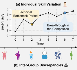
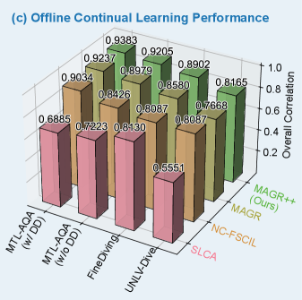
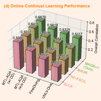
Figure 1: Motivation and challenges of CAQA. 1 and 1 illustrate the inherent limitations of conventional AQA methods, while 1 and 1 demonstrate that even strong CL baselines exhibit large performance gaps on CAQA benchmarks in both offline and online settings.

To this end, Continual Learning (CL) [13] provides a principled framework for adapting models to evolving distributions while retaining previously acquired knowledge. However, most CL research has focused on classification tasks [14, 15, 16], whereas its extension to AQA requires continual score regression and remains largely unexplored. Bridging this gap demands clear task formulation, benchmark construction, and customized evaluation protocols. In this work, we introduce Continual AQA (CAQA), a novel setting that extends CL to AQA tasks by confronting the dilemma between capturing fine-grained motion cues through continual adaptation and maintaining stability under non-stationary score distributions.

The complexity of CAQA poses unique challenges that render even strong CL baselines ineffective when applied directly (see Figs. 1 and 1). Existing PTM-based CL methods typically follow two paradigms: (i) extensive base-session adaptation followed by feature freezing, or (ii) Parameter-Efficient Fine-Tuning (PEFT) for continual updates [17, 15, 18]. While both strategies have shown success in classification, their limitations become evident in CAQA. First, the high cost of expert annotations [19] makes large-scale base-session adaptation impractical. Second, unlike coarse-grained classification, AQA relies on subtle motion cues, meaning frozen features without adequate adaptation fail to generalize across evolving distributions [20, 21]. Finally, although PEFT provides a lightweight mechanism for continual updates, the substantial domain gap between upstream recognition and downstream fine-grained AQA renders such adapters insufficient. Our empirical study (see Sect. III-B) demonstrates that Full-Parameter Fine-Tuning (FPFT) consistently outperforms PEFT, suggesting its necessity to CAQA.

To investigate this observation, we conduct an in-depth theoretical analysis under a representative, storage-efficient feature replay strategy, and obtain two key insights. First, while FPFT is effective for realigning representations, repeated use in long-term continual adaptation risks severe overfitting. Second, continual distribution shifts cause replayed features to drift from the evolving data manifold, undermining rehearsal effectiveness. Inspired by these, we propose Adaptive Manifold-Aligned Graph Regularization (MAGR++), an innovative framework that addresses both overfitting and distribution shift in CAQA. MAGR++ employs a layer-adaptive fine-tuning strategy that constrains shallow layers from drifting while fully tuning deeper ones to embrace session-specific variations, with the boundary determined adaptively. It further incorporates a manifold projector that maps historical features into the current representation space and a graph regularizer that enforces both local and global consistency between feature and quality spaces, enabling reliable replay and regression. Together, these modules allow MAGR++ to achieve effective continual adaptation while maintaining stability.

We establish four CAQA benchmarks from three AQA datasets, with tailored evaluation metrics and strong baselines for systematic cross-dataset comparison. Experiments across both offline and online CAQA settings demonstrate that MAGR++ achieves state-of-the-art performance, surpassing the strongest baseline by 1.6%–6.5% offline and 4.0%–21.8% online, with average gains of 3.6% and 12.2%, respectively.

This work substantially extends our preliminary version MAGR [22]. Beyond a complete rewriting of the manuscript, MAGR++ advances the prior work in three key aspects. First, we establish a solid theoretical foundation that formalizes the challenges of CAQA and clarifies the principles guiding our design. Second, we propose a theoretically grounded solution that tackles the stability–adaptability dilemma through layer-adaptive fine-tuning and an asynchronous two-step feature rectification pipeline, providing a principled framework rather than an ad-hoc extension. Third, we broaden the empirical validation by incorporating both offline and online CAQA across diverse protocols and datasets, offering comprehensive evidence of robustness and generality.

Overall, our contributions can be summarized as follows:

• We introduce the first formulation of CAQA to explicitly tackle non-stationary action quality distributions.

• We develop a theoretical framework that reveals two fundamental challenges of CAQA, i.e., overfitting from repeated FPFT and feature drift under feature replay.

• We propose a theoretically grounded CAQA method with adaptive FPFT for robust representation learning and two-step rectification for coherent feature alignment.

• We conduct extensive experiments on four CAQA benchmarks. Our method achieves consistently state-of-the-art performance in both offline and online settings.

II Related Work

Action Quality Assessment. AQA aims to automatically evaluate the objective execution quality of human actions, spanning numerous applications in sports scoring [23, 24, 25, 26, 27], rehabilitation [8], and skill assessment [28]. A major challenge is the scarcity of annotated labels [19], since reliable quality scores demand domain expertise. To address this, most approaches [29, 30, 31] leverage PTMs (e.g., I3D [11]) to extract strong visual features and then regress quality scores either via direct regression [32] or contrastive regression [33]. Ranking-based skill assessment methods [34, 35] further alleviate annotation costs by comparing relative performance instead of relying on absolute scores. Another core difficulty lies in fine-grained temporal parsing, as PTMs are optimized for coarse action recognition while AQA demands temporal sensitivity. To this end, strategies such as continual pretraining [36], regularization [21, 20], and human-centric cues [37, 38] have been proposed to enhance feature representations. Furthermore, non-stationary variations across tasks pose additional challenges for CAQA. While recent works attempt to mitigate this by freezing backbone features [39], such designs restrict adaptation capacity and often overlook skill variations within the same action, where subtle distribution shifts make fine-grained evaluation more difficult. In this work, we address these challenges by designing a framework that both adapts to evolving task distributions and preserves discriminative skill-related cues, enabling AQA in realistic evolving scenarios.

Continual Learning. CL [40, 13] enables models to acquire new knowledge from a stream of tasks without forgetting previous ones. This capability is particularly valuable in real-world applications such as robotics, surveillance, and other dynamic vision domains [17]. The main challenge is to avoid catastrophic forgetting of previously learned knowledge. Current efforts can be broadly divided into constraint-based and replay-based methods. Constraint-based methods such as SI [41], EWC [42], and LwF [43] impose regularization to preserve old knowledge without storing past data, but often suffer from limited scalability. Replay-based methods, by contrast, achieve stronger retention via exemplar storage (e.g., MER [44], DER++ [45], TOPIC [46], and GEM [47]), which raises memory and privacy concerns. More recently, feature replay has emerged as a lightweight and privacy-preserving alternative (e.g., SLCA [48, 49], NC-FSCIL [50], FS-Aug [39], and MAGR [22]). However, applying feature replay in domains like AQA is challenging due to significant domain gaps, and continual adaptation of the backbone often induces manifold shifts, misaligning old and new feature distributions. Motivated by these, our work adopts feature replay as the primary technical route of CAQA while introducing adaptive strategies to alleviate feature misalignment.

III Preliminaries of AQA and CAQA

In this section, we describe the problem formulation of AQA and CAQA, empirically investigate FPFT and PEFT under these settings, and provide an in-depth theoretical analysis with storage-efficient feature replay, which yields key implications for the design of MAGR++.

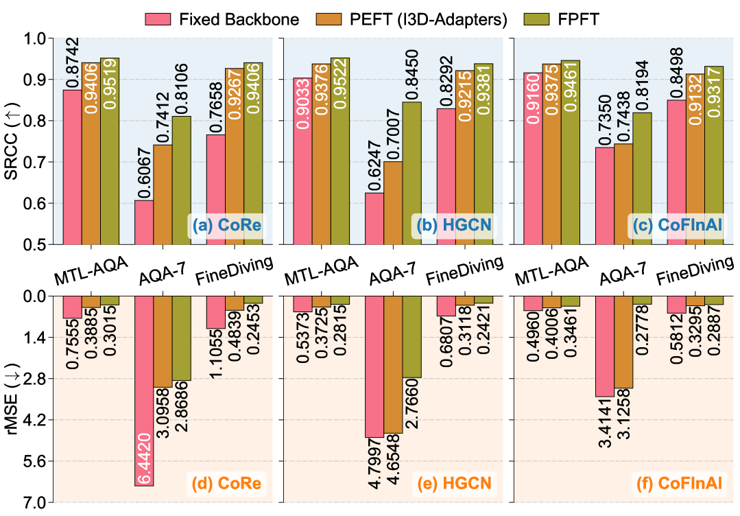
Figure 2: SRCC and rMSE comparison of fixed backbone, PEFT (I3D-Adapters), and FPFT in representative AQA tasks.

III-A Task Definition of AQA and CAQA

In AQA, the goal is to assign a quantitative score $\hat{y}\in\mathbb{R}$ to a video $\mathbf{x}\in\mathbb{R}^{F\times H\times W\times 3}$, where $F$, $H$, and $W$ denote the number of frames, height, and width. A backbone $f$ extracts features $\bm{h}=f(\mathbf{x})$, and a regressor $g$ predicts scores $\hat{y}=g(\bm{h})$, trained on a labeled dataset $\mathcal{D}_{\text{train}}=\{(\mathbf{x}_{n},y_{n})\}_{n=1}^{N}$. Traditional AQA assumes that both $\mathcal{D}_{\text{train}}$ and the parameters $\bm{\theta}_{f},\bm{\theta}_{g}$ remain fixed once trained. In practice, however, new actions, user populations, and individual variations continually emerge, leading to shifts in the underlying distribution. We therefore define CAQA: given a sequence of datasets $\{\mathcal{D}_{\text{train}}^{t}\}_{t=1}^{T}$ across sessions, the backbone $f^{t}$ and regressor $g^{t}$ are updated in each session to adapt to new data while retaining past knowledge. For clarity, we omit parameter dependence (e.g., $\bm{\theta}_{f}^{t},\bm{\theta}_{g}^{t}$) in the notation when referring to session $t$.

A critical challenge in CAQA is catastrophic forgetting, where learning from new data degrades performance on previous sessions. Rehearsal [13] is a simple yet effective remedy that stores and replays past samples. To this end, CAQA employs the storage-efficient feature replay [50], which maintains a memory bank $\mathcal{M}$ containing only a small set of representative latent embeddings $\bm{h}$ from previous sessions. Building on this, we define the CAQA objective as:

$$\min_{\bm{\theta}_{f}^{t},\,\bm{\theta}_{g}^{t}}~\mathcal{L}_{\text{D}}+\mathcal{L}_{\text{M}},$$ (1)

where $\mathcal{L}_{\text{D}}$ denotes the regression loss on the current session data $\mathcal{D}_{\text{train}}^{t}$, and $\mathcal{L}_{\text{M}}$ represents the replay loss on the memory bank $\mathcal{M}$. This joint objective enables the model to incrementally refine its assessment ability across sessions while effectively retaining previously acquired knowledge.

III-B Empirical Study of PEFT and FPFT for AQA

PEFT techniques [18], such as prompts, LoRA and adapters, are effective when upstream models are strong and downstream tasks are simple, as they require only minimal adaptation. In AQA, however, upstream models pretrained on coarse-grained action recognition are poorly aligned with the fine-grained motion cues essential for quality assessment [20, 21], yet the roles of PEFT and FPFT remain largely underexplored.

To close this gap, we adopt representative baselines for a fair empirical comparison. Since PEFT in AQA has only been explored with adapters, we use I3D-Adapters as its representative. Concretely, we compare fixed backbone (no adaptation), PEFT with I3D-Adapters [36], and FPFT across three benchmarks (MTL-AQA [31], AQA-7 [24], FineDiving [23]) with three prediction heads: CoRe [30], HGCN [32], and CoFInAl [20]. As shown in Fig. 2, FPFT consistently achieves superior performance in both SRCC (defined in Eq. 12) and rMSE [19] across all datasets and models. Compared with the fixed backbone, FPFT yields average gains of $+$3.33% SRCC and $-$31.23% rMSE, confirming that upstream features are poorly aligned for AQA. Compared with PEFT, FPFT achieves average gains of $+$2.11% SRCC and $-$14.25% rMSE, with the most significant improvement on AQA-7 ($+$5.89% SRCC, $-$44.21% rMSE), and smaller yet consistent benefits on MTL-AQA ($+$0.23% SRCC, $+$4.31% rMSE) and FineDiving ($+$0.22% SRCC, $-$2.85% rMSE), demonstrating that lightweight adapters cannot fully bridge the upstream–downstream gap.

To place these findings in a broader context, we categorize fine-tuning choices by the relative strengths of upstream models and downstream tasks, as shown in Fig. 3. We further provide an in-depth theoretical analysis as follows.

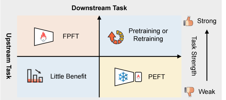
Figure 3: PEFT works well when upstream models are strong and downstream tasks are simple. FPFT does the opposite, as in AQA.

III-C Theoretical Analysis of FPFT with Feature Replay

Why FPFT Matters for AQA. As shown in Sect. III-B, FPFT consistently outperforms PEFT in AQA, though prior results mainly concern adapters. Theorem 1 generalizes this finding by showing that all PEFT methods suffer a projection gap: when the downstream optimum lies outside the restricted subspace, PEFT updates incur strictly positive excess risk under a curvature-induced metric, whereas FPFT avoids this.

Theorem 1

Let the upstream model $\phi_{\bm{\theta}_{\text{up}}}$ denote a pre-trained AQA scorer on a source domain $\mathcal{D}_{\text{up}}$ (typically large-scale action recognition), and define the downstream task on a target AQA domain $\mathcal{D}_{\text{down}}$ with a distinct data distribution. The goal is to adapt $\phi_{\bm{\theta}_{\text{up}}}$ by minimizing the downstream risk $R_{\text{down}}(\bm{\theta})=\mathbb{E}_{(x,y)\sim\mathcal{D}_{\text{down}}}\ell(\phi_{\bm{\theta}}(x),y)$, where $\bm{\theta}_{\text{down}}^{\star}=\arg\min_{\bm{\theta}}R_{\text{down}}(\bm{\theta})$. Following the unified view of PEFT methods [51], prompt tuning, adapter tuning, and LoRA share a common low-rank formulation. Taking LoRA as an example, updates are restricted to a low-rank subspace $\mathcal{S}:=\mathrm{range}(\mathbf{U})\subset\mathbb{R}^{d}$ via $\bm{\theta}=\bm{\theta}_{\text{up}}+\mathbf{U}\bm{\alpha}$, with $\mathbf{U}\in\mathbb{R}^{d\times r}$ and $\mathrm{rank}(\mathbf{U})=r\!\ll\!d$, while FPFT allows full-space updates. The upstream Jacobian $\mathbf{J}_{\text{up}}(x):=\nabla_{\bm{\theta}}\phi_{\bm{\theta}_{\text{up}}}(x)$ measures the local sensitivity of outputs to parameters, and its Neural Tangent Kernel (NTK)-style Gram matrix $\mathbf{\Sigma}_{0}:=\mathbb{E}_{x\sim\mathcal{D}_{\text{down}}}[\mathbf{J}_{\text{up}}(x)\mathbf{J}_{\text{up}}(x)^{\top}]\succeq 0$ characterizes the curvature and geometry around $\bm{\theta}_{\text{up}}$. Assume:

• (Curvature) The loss $\ell(\cdot,y)$ is twice differentiable and locally strongly convex, i.e., $\ell^{\prime\prime}(z,y)\geq\mu>0$, ensuring a quadratic lower bound on the risk landscape.

• (Nondegeneracy) The curvature of $\mathbf{\Sigma}_{0}$ on the orthogonal complement $\mathcal{S}^{\perp}$ is positive, i.e., $\lambda_{\min}(\mathbf{\Sigma}_{0}\!\mid_{\mathcal{S}^{\perp}})>0$, ensuring that useful and stable descent directions exist consistently outside the PEFT subspace.

• (Linearization) There exist constants $\rho>0$ and $L_{\varepsilon}\!\geq\!0$ such that for all small perturbations $\bm{v}$ with $\|\bm{v}\|\!\leq\!\rho$, $\big|R_{\text{down}}(\bm{\theta}_{\text{up}}+\bm{v})-\widetilde{R}_{\text{down}}(\bm{v})\big|\leq\tfrac{L_{\varepsilon}}{2}\|\bm{v}\|^{2}$, where the linearized risk is $\widetilde{R}_{\text{down}}(\bm{v})=\mathbb{E}_{(x,y)\sim\mathcal{D}_{\text{down}}}\!\ell\big(\phi_{\bm{\theta}_{\text{up}}}(x)+\mathbf{J}_{\text{up}}(x)^{\top}\bm{v},\,y\big)$, and both the restricted and full minimizers, $\bm{v}_{\mathcal{S}}=\arg\min_{\bm{v}\in\mathcal{S}}\widetilde{R}_{\text{down}}(\bm{v})$ and $\bm{v}^{\star}=\arg\min_{\bm{v}}\widetilde{R}_{\text{down}}(\bm{v})$, lie within the local region $\|\bm{v}\|\leq\rho$.

Under these assumptions, for any PEFT parameter $\bm{\alpha}$ (such that $\bm{v}=\mathbf{U}\bm{\alpha}\in\mathcal{S}$), the following holds:

$$R_{\text{down}}(\bm{\theta}_{\text{up}}+\mathbf{U}\bm{\alpha})-R_{\text{down}}(\bm{\theta}_{\text{down}}^{\star})\geq\tfrac{\mu}{2}\,\|\Pi_{\mathcal{S}^{\perp}}^{(\mathbf{\Sigma}_{0})}\bm{\Delta}\|_{\mathbf{\Sigma}_{0}}^{2}-C_{\varepsilon},$$ (2)

where $\bm{\Delta}:=\bm{\theta}_{\text{down}}^{\star}-\bm{\theta}_{\text{up}}$, $\|\bm{w}\|_{\mathbf{\Sigma}_{0}}^{2}:=\bm{w}^{\top}\mathbf{\Sigma}_{0}\bm{w}$, $\Pi_{\mathcal{S}^{\perp}}^{(\mathbf{\Sigma}_{0})}$ is the $\mathbf{\Sigma}_{0}$-orthogonal projection onto $\mathcal{S}^{\perp}$ (well-defined under assumption (A2)), and $C_{\varepsilon}:=\tfrac{L_{\varepsilon}}{2}(\|\bm{v}_{\mathcal{S}}\|^{2}+\|\bm{v}^{\star}\|^{2})$.

Eq. 2 indicates that PEFT suffers excess risk whenever the downstream optimum $\bm{\theta}_{\text{down}}^{\star}$ has a nonzero projection onto $\mathcal{S}^{\perp}$, the complement of its update subspace. The projection term $\|\Pi_{\mathcal{S}^{\perp}}^{(\mathbf{\Sigma}_{0})}\bm{\Delta}\|_{\mathbf{\Sigma}_{0}}^{2}$ measures the portion of adaptation inaccessible to PEFT under the curvature geometry of $\mathbf{\Sigma}_{0}$. In contrast, FPFT can align with the full descent direction, achieving lower risk. A detailed proof of Theorem 1 is provided in Appendix A.

When FPFT Meets Feature Replay. While Theorem 1 shows the advantage of FPFT over PEFT in static transfer, the CAQA setting requires continual adaptation to evolving distributions. In practice, feature replay [50] is widely adopted to mitigate forgetting with limited extra memory. However, combining FPFT with feature replay introduces new risks: FPFT may induce overfitting due to large parameter shifts, and historical features stored in memory can drift away from the representations produced by the continually updated backbone. To better understand these challenges, Theorem 2 formalizes FPFT under replay and establishes stability conditions.

Theorem 2

Let $f_{\bm{\theta}_{f}}:\mathcal{X}\!\to\!\mathbb{R}^{m}$ be the encoder (backbone), $g_{\bm{\theta}_{g}}:\mathbb{R}^{m}\!\to\!\mathbb{R}$ be the output head, and the full model be $\phi_{\bm{\theta}}:=g_{\bm{\theta}_{g}}\circ f_{\bm{\theta}_{f}}$, where $\bm{\theta}=\{\bm{\theta}_{f},\bm{\theta}_{g}\}$. At session $t$, parameters update from $\bm{\theta}^{t-1}$ to $\bm{\theta}^{t}$ by FPFT on new data $\mathcal{D}_{t}$ while replaying a memory buffer $\mathcal{M}_{t-1}$. We denote the update vector as $\bm{\Delta}_{t}:=\bm{\theta}^{t}-\bm{\theta}^{t-1}$ and its associated step size as $\Delta_{t}:=\|\bm{\Delta}_{t}\|$. Assume:

• (Loss Smoothness) The loss $\ell(\cdot,y)$ (e.g., MSE or KL divergence) is $1$-Lipschitz continuous with respect to its scalar input, ensuring that small prediction changes lead to bounded loss variation.

• (Head Regularity) For any parameter $\bm{\theta}_{g}$, the prediction head $g_{\bm{\theta}_{g}}$ is $L_{g}$-Lipschitz continuous with respect to its feature input, limiting sensitivity in score prediction caused by feature perturbations.

• (Backbone Stability) The backbone mapping $f_{\bm{\theta}_{f}}$ satisfies $\|f_{\bm{\theta}^{\prime}_{f}}(x)-f_{\bm{\theta}_{f}}(x)\|\leq L_{f}\,\|\bm{\theta}^{\prime}_{f}-\bm{\theta}_{f}\|$ uniformly for all $x\in\mathcal{X}$ and parameters $\bm{\theta}_{f},\bm{\theta}^{\prime}_{f}$, ensuring representation smoothness during encoder updates.

• (Model Continuity) The overall mapping $\phi_{\bm{\theta}}=g_{\bm{\theta}_{g}}\!\circ\!f_{\bm{\theta}_{f}}$ is uniformly continuous, satisfying $\|\phi_{\bm{\theta}^{\prime}}(x)-\phi_{\bm{\theta}}(x)\|\leq L_{\phi}\,\|\bm{\theta}^{\prime}-\bm{\theta}\|$, which guarantees bounded prediction drift under finite-step updates.

Under these regularity and stability conditions, for any past task $k<t$, the expected forgetting satisfies

$$\mathbb{E}\!\left[\psi_{t}(k)\right]\;\;\lesssim\;\;L_{g}L_{f}\,\Delta_{t}\;+\;C\,L_{\phi}\,\Delta_{t}\;+\;E_{\text{opt}},$$ (3)

where $\psi_{t}(k)$ denotes the forgetting on task $k$ after session $t$, the first term quantifies the replay-drift contribution from feature mismatch, the second term reflects the growth of the hypothesis class (for some constant $C>0$), and $E_{\text{opt}}\geq 0$ accounts for the residual optimization error at session $t$.

Eq. 3 shows that FPFT’s flexibility comes at the cost of stability: large updates $\Delta_{t}$ amplify both replay drift ($L_{g}L_{f}\Delta_{t}$) and generalization growth ($CL_{\phi}\Delta_{t}$), leading to potential overfitting and forgetting. Moreover, stale features from the old encoder deviate from the updated one, weakening replay supervision. These findings motivate the layer-adaptive tuning and feature rectification in MAGR++, which jointly constrain $\Delta_{t}$ and reduce feature drift for stable continual adaptation. A detailed proof of Theorem 2 is deferred to Appendix B.

Theorem 1 shows that FPFT strictly dominates PEFT by avoiding projection gaps, yet Theorem 2 further reveals two crucial risks in CAQA: (i) FPFT may suffer from overfitting as the hypothesis class grows across sessions, and (ii) feature replay is vulnerable to representation drift when old features become misaligned with the updated backbone. In the original MAGR [22], synchronous projector training exacerbates this misalignment, leading to unstable replay correction.

To address these challenges, MAGR++ introduces two key improvements: (i) layer-adaptive fine-tuning, which constrains updates on low-level layers while fully tuning high-level ones, thereby balancing stability and adaptability; and (ii) asynchronous feature rectification, which allows the backbone and projector to converge before replay correction, preventing noisy updates and ensuring robust continual adaptation.

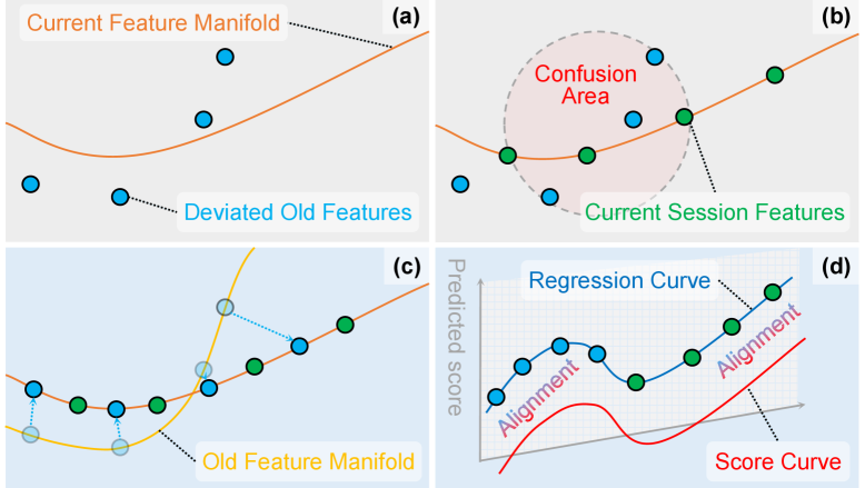
Figure 4: Core idea of MAGR++: (a) Old features (blue circles) deviate from the current manifold (orange curve) due to manifold shift; (b) Mixing old and new features (green circles) leads to confusion in score regression; (c) The manifold projector translates old features from the previous manifold (yellow curve) to the current one; (d) The feature space is further aligned with the quality score space.

IV Adaptive Manifold-Aligned Graph Regularization (MAGR++)

This section presents the design of our proposed MAGR++ for CAQA. We first introduce the task definition, motivation, and overall architecture, and then describe the core modules. The training strategy that integrates these components into a CL system is presented in Appendix C.

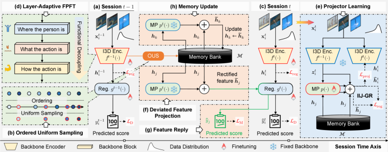
Figure 5: Overview of MAGR++. At the end of session $t-1$ 5, representative features are selected via Ordered Uniform Sampling (OUS, 5) and stored in the memory bank $\mathcal{M}$. At the start of session $t$ 5, the backbone is adapted with layer-adaptive FPFT 5 to balance stability and plasticity. A Manifold Projector (MP) is then trained 5 to align old features with the evolving feature space 5, enabling effective replay and regressor adaptation 5. Finally, the memory bank is refreshed with rectified old features and newly sampled prototypes 5.

IV-A Motivation and Framework Overview

Addressing CAQA Challenges with MAGR++. As discussed in Sect. III, CAQA poses a dilemma for CL: fine-tuning the backbone is essential for adapting to new sessions, yet it inevitably causes feature manifold shift and catastrophic forgetting. As illustrated in Fig. 4, this shift causes stored feature prototypes (blue circles) to deviate from the new feature manifold (orange curve), making them ineffective for reply (see Fig. 4) and prone to confusing score regression when mixed with current features (see Fig. 4). These challenges undermine replay-based methods and highlight the need for shift-aware adaptation. To address this, MAGR++ introduces a two-step solution: (i) mapping old features from their previous manifold (yellow curve) onto the current session’s manifold (see Fig. 4); and (ii) readjusting the translated distribution for optimal alignment with target scores (see Fig. 4).

Framework Overview. Fig. 5 depicts the overall pipeline of MAGR++. At the end of session $t-1$ (see Fig. 5), Ordered Uniform Sampling (OUS, see Fig. 5) stores representative features in the memory bank $\mathcal{M}$ by sorting samples by quality scores and uniformly selecting them across the score range, ensuring diverse coverage. At the beginning of each new session $t$ (see Fig. 5), the backbone is adapted to the new data distribution via layer-adaptive FPFT (see Fig. 5). Next, the Manifold Projector (MP) is trained to align session-wise feature spaces (see Fig. 5) by using paired features from the frozen backbone $f^{t-1}$ and the updated backbone $f^{t}$, learning a mapping from the old space to the new one. Additionally, an Intra-Inter-Joint Graph Regularization (IIJ-GR) promotes feature alignment across sessions. The regressor is jointly trained on rectified old features and new features (see Fig. 5), enabling adaptation to new data while retaining previously acquired knowledge. Finally, after regressor training, old features are first updated via MP to align with the current feature space (see Fig. 5), and new prototypes from session $t$ are chosen and added to $\mathcal{M}$.

Formally, at session $t$, MAGR++ optimizes the backbone ($\bm{\theta}_{f}^{t}$), regressor ($\bm{\theta}_{g}^{t}$), and manifold projector ($\bm{\theta}_{p}^{t}$) by minimizing the following composite training objective:

$$\min_{\bm{\theta}_{f}^{t},\,\bm{\theta}_{g}^{t},\,\bm{\theta}_{p}^{t}} \ \mathcal{L}_{\text{D}}+\mathcal{L}_{\text{M}}+\lambda_{\text{tune}}\,\mathcal{L}_{\text{tune}}+\lambda_{\text{proj}}\,\mathcal{L}_{\text{proj}}+\lambda_{\text{reg}}\,\mathcal{L}_{\text{reg}}$$ (4)

s.t. $$\ \hat{y}_{i}^{t}=g^{t}(f^{t}(\mathbf{x}_{i}^{t})),~~(\mathbf{x}_{i}^{t},y_{i}^{t})\in\mathcal{D}^{t}_{\text{train}},$$

$$\ \hat{y}_{j}=g^{t}(p^{t}(\bm{h}_{j})),~~(\bm{h}_{j},y_{j})\in\mathcal{M}.$$

Here, $\mathcal{L}_{\text{D}}$ and $\mathcal{L}_{\text{M}}$ follow Eq. 1, $\mathcal{L}_{\text{tune}}$ is the FPFT loss (see Eq. 6 in Sect. IV-B), and $\mathcal{L}_{\text{proj}}$ (see Eq. 8 in Sect. IV-C) and $\mathcal{L}_{\text{reg}}$ (see Eq. 11 in Sect. IV-D) regularize the projector and regressor, respectively. The coefficients $\lambda_{\text{tune}}$, $\lambda_{\text{proj}}$, and $\lambda_{\text{reg}}$ balance the corresponding loss terms.

IV-B Stability–Adaptability Balance via Layer-Adaptive FPFT

A central challenge in CAQA is the stability–adaptability dilemma: FPFT provides strong adaptation to new sessions but risks overfitting and catastrophic forgetting. Inspired by prior findings in vision representation learning [52], we leverage the hierarchical functionality of pretrained backbone: shallow layers capture spatial cues (where), middle layers encode semantics (what), and deeper layers model execution quality (how). Since AQA depends primarily on fine-grained motion quality, we propose layer-adaptive FPFT (see Fig. 6), which constrains shallow layers for stability while fully fine-tuning deeper layers for adaptability. Adaptive layer selection identifies the optimal boundary, and constrained full tuning regularizes updates, systematically balancing robustness and flexibility. Unlike previous CL methods such as first-session adaptation and continual PEFT [17, 18, 15, 53], our novelty lies in exploiting the intrinsic hierarchical decomposition of representations to explicitly balance stability and adaptability in CAQA, offering a principled solution applicable beyond this domain.

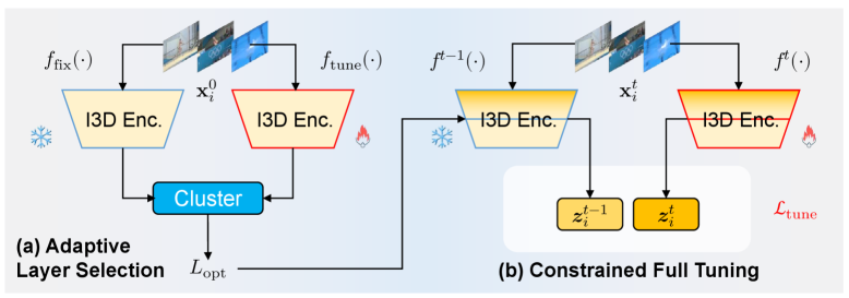
Figure 6: Illustration of layer-adaptive FPFT.

Adaptive Layer Selection. The key to layer-adaptive FPFT lies in identifying the optimal boundary between stable and adaptive layers. Exhaustive grid search is infeasible since it requires future session data and incurs prohibitive cost. Instead, we exploit only base-session data to guide boundary selection, preventing information leakage. As shown in Fig. 6, we evaluate the abstraction degree encoded at each layer by treating clustering quality as a proxy for feature abstraction, denoted as $\mathcal{C}^{l}$ for the $l$-th layer. Shallower layers dominated by low-level appearance cues generally yield noisy and less separable structures, whereas deeper layers encode more abstract and quality-aware features that are easier to cluster by action scores. For each layer $l$, we compute the Davies–Bouldin index from both the frozen backbone $f_{\text{fix}}$ and the fine-tuned backbone $f_{\text{tune}}$, and define the abstraction ratio as $r^{l}=\mathcal{C}^{l}_{\text{tune}}/\mathcal{C}^{l}_{\text{fix}}$. The key intuition is that $r^{l}\leq 1$ indicates no gain, or even degradation, from fine-tuning, suggesting that the layer is still dominated by low-level cues, whereas $r^{l}>1$ signifies improved separability and abstraction through fine-tuning. Accordingly, the optimal boundary is determined as:

$$L_{\text{opt}}=\min\big\{l\in\{1,\dots,L\}\;|\;r^{l}>1+\epsilon\big\},$$ (5)

where $\epsilon$ is a small margin (e.g., 0.05) introduced to enhance robustness against noise. Layers below $L_{\text{opt}}$ are constrained to remain stable, while deeper layers are fully fine-tuned to adapt to evolving quality distributions. This principled criterion eliminates future-data dependence, avoids costly grid search, and provides a robust mechanism for balancing stability and adaptability in CAQA. As shown in Fig. 9, the layer boundaries selected by our method are consistent with those obtained via exhaustive grid search, verifying its effectiveness.

Constrained Full Tuning. During the current session $t$, we constrain the backbone’s updates for layers below $L_{\text{opt}}$ when adapting the backbone $f^{t}$ (see Fig. 6). Given current session data $\mathbf{x}_{i}^{t}$, we obtain paired features $\bm{z}_{i}^{t,l}$ from $f^{t}$ and $\bm{z}_{i}^{t-1,l}$ from the previous backbone $f^{t-1}$ at layer $l<L_{\text{opt}}$. We then enforce consistency between features across sessions using a feature-matching loss, which is:

$$\mathcal{L}_{\text{tune}}=\frac{1}{N_{t}}\sum_{i=1}^{N_{t}}\sum_{l<L_{\text{opt}}}\big\|\bm{z}_{i}^{t,l}-\bm{z}_{i}^{t-1,l}\big\|_{2}^{2},$$ (6)

where $N_{t}$ is the number of samples in the current session and $\bm{z}_{i}^{t,l}$ denotes the feature from layer $l$ at session $t$. Unlike freezing features entirely, this soft constraint still permits shallow layers to undergo limited adaptation, as suggested by Fig. 9, while effectively preventing uncontrolled drift. This design stabilizes generic low-level representations without suppressing their necessary refinement, thereby balancing stability and adaptability during FPFT. Interestingly, our experiments further show that applying the constraint only at layer $L_{\text{opt}}-1$ is sufficient to achieve stable performance, offering a lightweight yet effective regularization strategy.

IV-C Deviated Feature Translation via Manifold Projector

As identified in Sect. III, CAQA suffers from manifold shift under FPFT, as features extracted from earlier sessions become inconsistent with the updated backbone, causing replayed samples to misalign with the current representation and degrade regressor performance. Existing strategies remain insufficient. Experience replay [45] depends on raw inputs and raises storage and privacy concerns. Backbone freezing [50] preserves stability but hinders adaptation. Alignment-based corrections [48] only partially capture evolving shifts. To this end, we introduce the Manifold Projector (MP), which estimates the manifold shift between adjacent sessions and translates deviated features into the current representation space without requiring raw inputs.

Projector Learning. The key to MP lies in estimating the manifold shift without accessing raw data from previous sessions. We cast this as a self-supervised prediction problem using only current-session inputs. As shown in Fig. 5, at the start of session $t$ we freeze the previous backbone $f^{t-1}$ and compute initial features $\bm{z}_{j}^{t}=f^{t-1}(\mathbf{x}_{j}^{t})$ for each current sample $\mathbf{x}_{j}^{t}$. We then train a projector $p(\cdot)$ to predict the updated features produced by the adapting backbone $f^{t}$, which is:

$$\bm{\hat{h}}_{j}^{t}=\bm{z}_{j}^{t}+p(\bm{z}_{j}^{t}),$$ (7)

where the residual connection stabilizes optimization. The projector is optimized by minimizing the discrepancy between the predicted features $\bm{\hat{h}}_{j}^{t}$ and the actual updated features $\bm{h}_{j}^{t}=f^{t}(\mathbf{x}_{j}^{t})$, which is:

$$\mathcal{L}_{\text{proj}}=\frac{1}{N_{t}}\sum_{j}\|\bm{h}_{j}^{t}-\bm{\hat{h}}_{j}^{t}\|_{2}^{2},$$ (8)

where $N_{t}$ is the number of samples in session $t$, and $\|\cdot\|_{2}^{2}$ denotes the mean squared error. In parallel, old features fetched from the memory bank are updated via the projector and used to compute a regularization loss with respect to $\bm{\hat{h}}_{j}^{t}$, further constraining projector learning (detailed in Sect. IV-D). This design enables the projector to capture representation shifts effectively without requiring access to old data.

Deviated Feature Projection. Once trained with sufficient coverage of the current session data, the projector is applied to translate old features from previous sessions into the current representation space. For an old feature $\bm{h}_{i}^{s}$ stored in memory ($s<t$), the corrected feature is computed as:

$$\bm{h}_{i}^{s}\leftarrow\bm{h}_{i}^{s}+p(\bm{h}_{i}^{s}).$$ (9)

This translation aligns old features with the updated manifold, ensuring stable replay that alleviates catastrophic forgetting.

IV-D Feature Alignment via Intra-Inter-Joint Graph Regularizer

While MP translates old features into the current representation space, it does not ensure that the overall feature distribution remains aligned with the quality score distribution (see Fig. 4). Existing graph-based CL methods [46] often rely on Euclidean distances, which fail to capture the geodesic structure of quality relationships and thus distort feature–score alignment (see Fig. 7). Furthermore, features from different sessions may suffer from inconsistent scaling, which disrupts the relative ordering of quality scores and confuses regression. To address these issues, we propose the Intra-Inter-Joint Graph Regularizer (IIJ-GR), which explicitly enforces both local (intra-session) and global (inter-session) consistency between the feature and score spaces, as shown in Fig. 7. The key innovation lies in leveraging angular distances on a unit hypersphere (see Fig. 7), together with a distance matrix partitioning strategy (see Fig. 7) that provides a principled mechanism to preserve the geometric structure of quality relationships across sessions, thereby enhancing both stability and accuracy in CAQA.

Distance Matrix Partitioning. Given a mini-batch of old features $\bm{h}_{i}^{s}$ from the memory bank and $\bm{h}_{j}^{t}$ from the current session, we form a joint feature matrix $\mathbf{H}=[\bm{h}_{1}^{s},\dots,\bm{h}_{b_{1}}^{s},\bm{h}_{1}^{t},\dots,\bm{h}_{b_{2}}^{t}]$. All features are normalized onto a unit hypersphere, where each row of $\tilde{\mathbf{H}}$ has unit length. Their pairwise angular distances are:

$$\mathbf{A}=\arccos\!\left(\tilde{\mathbf{H}}\tilde{\mathbf{H}}^{\top}\right).$$ (10)

Compared to Euclidean distance, angular distance better preserves the geodesic structure of semantic similarity [54], which is crucial for reflecting fine-grained quality cues. The resulting matrix $\mathbf{A}$ is then partitioned into four sub-blocks corresponding to intra-session relations in past data, intra-session relations in current data, and inter-session relations across the two. This partitioning disentangles local (within-session) and global (cross-session) dependencies, enabling structured supervision that balances stability and adaptability in distribution alignment.

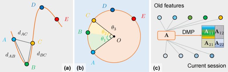
Figure 7: Illustrations of IIJ-GR: 7 Euclidean distance, 7 Angular distance, and 7 Distance Matrix Partitioning (DMP).

Graph Regularization. To align the feature geometry with quality relationships, we construct a score distance matrix $\mathbf{S}=\bm{y}-\bm{y}^{\top}$, where $\bm{y}$ denotes the quality labels of the joint batch. We then define the regularization loss as:

$$\mathcal{L}_{\text{reg}}=\|\mathbf{A}-\mathbf{S}\|_{2}^{2}+\sum_{i=1}^{2}\sum_{j=1}^{2}\|\mathbf{A}_{ij}-\mathbf{S}_{ij}\|_{2}^{2}.$$ (11)

By jointly optimizing the global distance matrix $\mathbf{A}$ and its sub-blocks against $\mathbf{S}$, IIJ-GR enforces alignment between feature distances and score relationships at both intra- and inter-session levels. This design preserves local ranking consistency within each session while maintaining global comparability across sessions, ensuring that rectified features remain semantically meaningful for continual regression.

TABLE I: Offline performance comparison. The primary metric is $\rho_{\text{avg}}$, with Joint Training as the Upper Bound (UB) and Sequential FT as the Lower Bound (LB). Best results are highlighted in bold. $\uparrow$: higher is better; $\downarrow$: lower is better.

a MTL-AQA (default, w/o difficulty label)

Method	Publisher	Memory	$\rho_{\text{avg}}$ ($\uparrow$)	$\rho_{\text{aft}}$ ($\downarrow$)	$\rho_{\text{fwt}}$ ($\uparrow$)
Joint Training (UB)	-	None	0.9360	-	-
Sequential FT (LB)	-	None	0.5458	0.1524	$0.0538$
SI [41]	ICML’17	None	0.5526	0.2677	$0.0350$
EWC [42]	PNAS’17	None	0.2312	0.1553	$0.0343$
LwF [43]	TPAMI’17	None	0.4581	0.1894	$0.0490$
MER [44]	ICLR’19	Raw Data	0.8720	0.1303	$0.0625$
DER++ [45]	NeurIPS’20	Raw Data	0.8334	0.1775	$0.0433$
TOPIC [46]	CVPR’20	Raw Data	0.7693	0.1427	$0.1391$
GEM [47]	ICCV’21	Raw Data	0.8583	0.0950	$0.1429$
Feature MER	-	Feature	0.7283	0.2255	$0.0535$
SLCA [48]	ICCV’23	Feature	0.7223	0.1852	$0.1665$
NC-FSCIL [50]	ICLR’23	Feature	0.8426	0.1146	$0.0718$
FS-Aug [39]	TCSVT’24	Feature	0.8060	0.1456	$0.0790$
MAGR [22]	ECCV’24	Feature	0.8979	0.0223	$0.1914$
MAGR++ (Ours)	-	Feature	0.9205	0.0103	$0.1274$

b MTL-AQA (w/ difficulty)

Method	Publisher	Memory	$\rho_{\text{avg}}$ ($\uparrow$)	$\rho_{\text{aft}}$ ($\downarrow$)	$\rho_{\text{fwt}}$ ($\uparrow$)
Joint Training (UB)	-	None	0.9587	-	-
Sequential FT (LB)	-	None	0.8684	0.1418	$0.2282$
SI [41]	ICML’17	None	0.8678	0.2050	$0.2491$
EWC [42]	PNAS’17	None	0.8625	0.1267	$0.1776$
LwF [43]	TPAMI’17	None	0.7852	0.1501	$0.0912$
MER [44]	ICLR’19	Raw Data	0.9234	0.0832	$0.3089$
DER++ [45]	NeurIPS’20	Raw Data	0.9037	0.1230	$0.3122$
TOPIC [46]	CVPR’20	Raw Data	0.8782	0.1394	$0.2304$
GEM [47]	ICCV’21	Raw Data	0.8873	0.1707	$0.3127$
Feature MER	-	Feature	0.8785	0.2130	$0.2436$
SLCA [48]	ICCV’23	Feature	0.6885	0.2029	$0.0958$
NC-FSCIL [50]	ICLR’23	Feature	0.9034	0.0878	$0.1456$
FS-Aug [39]	TCSVT’24	Feature	0.9136	0.1280	$0.3145$
MAGR [22]	ECCV’24	Feature	0.9237	0.0615	$0.1944$
MAGR++ (Ours)	-	Feature	0.9383	0.0181	$0.3222$

c FineDiving (w/ dive number)

Method	Publisher	Memory	$\rho_{\text{avg}}$ ($\uparrow$)	$\rho_{\text{aft}}$ ($\downarrow$)	$\rho_{\text{fwt}}$ ($\uparrow$)
Joint Training (UB)	-	None	0.9075	-	-
Sequential FT (LB)	-	None	0.7420	0.1322	$0.2135$
SI [41]	ICML’17	None	0.6863	0.2330	$0.1938$
EWC [42]	PNAS’17	None	0.5311	0.3177	$0.1776$
LwF [43]	TPAMI’17	None	0.7648	0.0807	$0.2894$
MER [44]	ICLR’19	Raw Data	0.8276	0.1446	$0.2806$
DER++ [45]	NeurIPS’20	Raw Data	0.8285	0.1523	$0.2851$
TOPIC [46]	CVPR’20	Raw Data	0.8006	0.1344	$0.2744$
GEM [47]	ICCV’21	Raw Data	0.8309	0.0721	$0.2883$
Feature MER	-	Feature	0.4914	0.2354	$0.2344$
SLCA [48]	ICCV’23	Feature	0.8130	0.0920	$0.2453$
NC-FSCIL [50]	ICLR’23	Feature	0.8087	0.0203	$0.3404$
FS-Aug [39]	TCSVT’24	Feature	0.8123	0.1412	$0.2928$
MAGR [22]	ECCV’24	Feature	0.8580	0.0167	$0.2952$
MAGR++ (Ours)	-	Feature	0.8902	0.0090	$0.3915$

d UNLV-Dive

Method	Publisher	Memory	$\rho_{\text{avg}}$ ($\uparrow$)	$\rho_{\text{aft}}$ ($\downarrow$)	$\rho_{\text{fwt}}$ ($\uparrow$)
Joint Training (UB)	-	None	0.8460	-	-
Sequential FT (LB)	-	None	0.6307	0.2135	$0.3595$
SI [41]	ICML’17	None	0.1519	0.3822	$0.0220$
EWC [42]	PNAS’17	None	0.4096	0.2576	$0.3039$
LwF [43]	TPAMI’17	None	0.6081	0.1578	$0.3230$
MER [44]	ICLR’19	Raw Data	0.7397	0.1321	$0.0465$
DER++ [45]	NeurIPS’20	Raw Data	0.7206	0.1382	$-0.1773$
TOPIC [46]	CVPR’20	Raw Data	0.4085	0.2647	$0.1132$
GEM [47]	ICCV’21	Raw Data	0.6538	0.2322	$0.0270$
Feature MER	-	Feature	0.5675	0.1322	$0.1558$
SLCA [48]	ICCV’23	Feature	0.5551	0.1085	$0.3200$
NC-FSCIL [50]	ICLR’23	Feature	0.6458	0.0637	$-0.1677$
FS-Aug [39]	TCSVT’24	Feature	0.7374	0.0263	$-0.0742$
MAGR [22]	ECCV’24	Feature	0.7668	0.0827	$0.1227$
MAGR++ (Ours)	-	Feature	0.8165	0.0910	$0.3502$

TABLE II: Online performance comparison. The primary metric is $\rho_{\text{avg}}$, with Joint Training as the Upper Bound (UB) and Sequential FT as the Lower Bound (LB). Best results are highlighted in bold. $\uparrow$: higher is better; $\downarrow$: lower is better.

a MTL-AQA (default, w/o difficulty label)

Method	Publisher	Memory	$\rho_{\text{avg}}$ ($\uparrow$)	$\rho_{\text{aft}}$ ($\downarrow$)	$\rho_{\text{fwt}}$ ($\uparrow$)
Sequential FT (LB)	-	None	0.4926	0.0649	$-0.1416$
SI [41]	ICML’17	None	0.5243	0.0253	$0.0669$
EWC [42]	PNAS’17	None	0.5401	0.0303	$0.0850$
LwF [43]	TPAMI’17	None	0.5243	0.0170	$0.0797$
MER [44]	ICLR’19	Raw Data	0.5734	0.0394	$0.0262$
DER++ [45]	NeurIPS’20	Raw Data	0.5415	0.0146	$0.0857$
TOPIC [46]	CVPR’20	Raw Data	0.5116	0.0981	$0.0690$
GEM [47]	ICCV’21	Raw Data	0.5490	0.0612	$0.0972$
Feature MER	-	Feature	0.3571	0.1444	$-0.0213$
SLCA [48]	ICCV’23	Feature	0.4880	0.0430	$-0.0282$
NC-FSCIL [50]	ICLR’23	Feature	0.4971	0.0291	$-0.0463$
FS-Aug [39]	TCSVT’24	Feature	0.3322	0.0725	$-0.0581$
MAGR [22]	ECCV’24	Feature	0.5196	0.0337	$0.0282$
MAGR++ (Ours)	-	Feature	0.5618	0.0165	$0.0405$

b MTL-AQA (w/ difficulty label)

Method	Publisher	Memory	$\rho_{\text{avg}}$ ($\uparrow$)	$\rho_{\text{aft}}$ ($\downarrow$)	$\rho_{\text{fwt}}$ ($\uparrow$)
Sequential FT (LB)	-	None	0.6022	0.0647	$-0.0536$
SI [41]	ICML’17	None	0.6581	0.0803	$0.0429$
EWC [42]	PNAS’17	None	0.6371	0.1372	$0.0895$
LwF [43]	TPAMI’17	None	0.6416	0.0134	$0.3076$
MER [44]	ICLR’19	Raw Data	0.6290	0.0833	$0.0057$
DER++ [45]	NeurIPS’20	Raw Data	0.6444	0.1133	$0.0221$
TOPIC [46]	CVPR’20	Raw Data	0.6241	0.0916	$0.0258$
GEM [47]	ICCV’21	Raw Data	0.6422	0.0894	$0.0105$
Feature MER	-	Feature	0.6065	0.0472	$-0.0294$
SLCA [48]	ICCV’23	Feature	0.5980	0.0827	$-0.0266$
NC-FSCIL [50]	ICLR’23	Feature	0.5937	0.1006	$0.0181$
FS-Aug [39]	TCSVT’24	Feature	0.5339	0.0723	$-0.0108$
MAGR [22]	ECCV’24	Feature	0.6416	0.0134	$0.3076$
MAGR++ (Ours)	-	Feature	0.6676	0.0810	$-0.0126$

c FineDiving (w/o dive number)

Method	Publisher	Memory	$\rho_{\text{avg}}$ ($\uparrow$)	$\rho_{\text{aft}}$ ($\downarrow$)	$\rho_{\text{fwt}}$ ($\uparrow$)
Sequential FT (LB)	-	None	0.3970	0.0448	$0.0557$
SI [41]	ICML’17	None	0.4597	0.0149	$0.0553$
EWC [42]	PNAS’17	None	0.3222	0.0471	$0.0825$
LwF [43]	TPAMI’17	None	0.4230	0.0217	$0.1144$
MER [44]	ICLR’19	Raw Data	0.4116	0.0534	$0.0426$
DER++ [45]	NeurIPS’20	Raw Data	0.4358	0.0707	$0.1045$
TOPIC [46]	CVPR’20	Raw Data	0.4654	0.0978	$0.1086$
GEM [47]	ICCV’21	Raw Data	0.4414	0.0531	$0.1109$
Feature MER	-	Feature	0.1935	0.0998	$0.1559$
SLCA [48]	ICCV’23	Feature	0.3935	0.3360	$0.2346$
NC-FSCIL [50]	ICLR’23	Feature	0.3810	0.0079	$0.2518$
FS-Aug [39]	TCSVT’24	Feature	0.4266	0.0732	$0.1645$
MAGR [22]	ECCV’24	Feature	0.4641	0.0062	$0.2020$
MAGR++ (Ours)	-	Feature	0.5325	0.0094	$0.1227$

d UNLV-Dive

Method	Publisher	Memory	$\rho_{\text{avg}}$ ($\uparrow$)	$\rho_{\text{aft}}$ ($\downarrow$)	$\rho_{\text{fwt}}$ ($\uparrow$)
Sequential FT (LB)	-	None	0.2251	0.2592	$-0.1432$
SI [41]	ICML’17	None	0.3465	0.2211	$-0.3182$
EWC [42]	PNAS’17	None	0.3722	0.2631	$-0.3542$
LwF [43]	TPAMI’17	None	0.3981	0.2132	$-0.3913$
MER [44]	ICLR’19	Raw Data	0.2890	0.2222	$-0.3567$
DER++ [45]	NeurIPS’20	Raw Data	0.4291	0.1350	$-0.3106$
TOPIC [46]	CVPR’20	Raw Data	0.3874	0.2112	$-0.3454$
GEM [47]	ICCV’21	Raw Data	0.4094	0.2315	$-0.3773$
Feature MER	-	Feature	0.1308	0.2126	$-0.4571$
SLCA [48]	ICCV’23	Feature	0.3119	0.1641	$-0.3082$
NC-FSCIL [50]	ICLR’23	Feature	0.3136	0.1282	$-0.4892$
FS-Aug [39]	TCSVT’24	Feature	0.3639	0.1510	$-0.1555$
MAGR [22]	ECCV’24	Feature	0.4202	0.1947	$-0.0499$
MAGR++ (Ours)	-	Feature	0.5117	0.0959	$0.3927$

V Experiments

We conduct extensive experiments to evaluate the effectiveness and robustness of our proposed MAGR++ for CAQA. In addition, we provide supplementary experiments in Appendix D to further validate the generality of our approach.

V-A Experimental Setting

Datasets. We build CAQA benchmarks on three diving AQA datasets of varying scales and feature-shift levels (validated in Tab. III). MTL-AQA [24] contains 1412 samples across 16 diving events (male/female, single/double, 3m springboard, 10m platform), with detailed annotations of action categories, commentary, and AQA scores; 1059 samples are used for training and 353 for testing. FineDiving [23] includes 3000 dives from major competitions (Olympics, World Cup, etc.), annotated with 52 action types, 29 sub-action types, 23 difficulty levels, temporal boundaries, and both action and AQA scores; we adopt the official 75%/25% train/test split. UNLV-Dive [55] provides 370 videos (300 train and 70 test) from the 2012 London Olympics 10 m platform event, with final scores ranging from 21.6–102.6 and execution scores in [0, 30]. We focus on diving datasets in the main paper because they offer multiple well-annotated benchmarks with consistent action types, ensuring fair cross-dataset comparison. Results on other actions, such as UNLV-Vault [30], are provided in Appendix D to demonstrate generalization beyond diving while keeping the main analysis concise and focused.

CAQA Protocol. To simulate real-world skill variations, we introduce a grade-incremental setting for CAQA that couples regression and classification challenges. The continuous quality space is discretized into $G$ grade intervals, with $S$ samples per session to induce challenging score variations. Unlike the uniform and independent class space in traditional class-incremental tasks [56], our setting preserves contextual dependencies between adjacent grades. Here, grade order typically follows skill progression (with Fig. 10 analyzing task order effects), while the quality range also shifts across sessions. These challenges are compounded by the fine-grained regression nature of AQA, posing significant difficulties for lifelong learning in mitigating catastrophic forgetting.

CAQA Metrics. We propose innovative evaluation metrics tailored to the CAQA setting. Our design builds upon Spearman’s Rank Correlation Coefficient (SRCC) $\rho$, the standard metric in AQA for measuring the alignment between predicted scores $\hat{\bm{y}}$ and ground-truth scores $\bm{y}$. Given rank vectors $\bm{p}$ and $\bm{q}$ for $\bm{y}$ and $\hat{\bm{y}}$, SRCC is defined as:

$$\rho=\frac{\sum_{i}(p_{i}-\bar{p})(q_{i}-\bar{q})}{\sqrt{\sum_{i}(p_{i}-\bar{p})^{2}\sum_{i}(q_{i}-\bar{q})^{2}}},$$ (12)

where $\bar{p}$ and $\bar{q}$ are the mean ranks of $\bm{p}$ and $\bm{q}$. However, SRCC is highly sensitive to sample size, making simple averaging across sessions unreliable in CL scenarios. To address this, we introduce the overall correlation $\rho_{\text{avg}}$ as the primary CAQA metric, which aggregates predictions from all sessions into a single unified estimate, ensuring fairness and consistency across tasks. To further probe model stability and adaptability, we also report two auxiliary metrics: average forgetting $\rho_{\text{aft}}=\tfrac{1}{T-1}\sum_{t=1}^{T-1}\max_{i,j\in\{1,2,\cdots,T\}}(\rho_{i,t}-\rho_{j,t})$ and forward transfer $\rho_{\text{fwt}}=\tfrac{1}{T-1}\sum_{t=2}^{T}(\rho_{t-1,t}-\tilde{\rho}_{t})$, where $\rho_{i,j}$ denotes the correlation on the $j$-th test set after training up to task $i$ ($j\leq i$), and $\tilde{\rho}_{t}$ is the baseline correlation of a randomly initialized model on task $t$. Together, these three metrics provide a comprehensive assessment of CAQA in terms of accuracy, stability, and plasticity.

Implementation Details. All experiments are conducted on two Nvidia 4090 GPUs using PyTorch. We adopt the I3D backbone [11] with a score regression model [32]. Training is performed using Adam with a learning rate of $10^{-4}$ and weight decay of $10^{-5}$, run for up to 50 epochs in the offline setting, and for 1 epoch in the online setting. To emulate real-world constraints of limited data streams and label scarcity, we configure the incremental setting with $G=5$ and $S=20$, using batch size $b_{1}=5$ and mini-batch size $b_{2}=3$. The remaining data are reserved for base-session adaptation, providing a stable foundation before incremental updates. Batch normalization layers in the backbone are frozen to mitigate small-batch effects. MP is implemented as a two-layer MLP that learns residual feature shifts between old and new manifolds, which can be effectively captured without complex architectures. All losses are normalized to remove scale mismatch, so $\lambda_{\text{tune}}$, $\lambda_{\text{proj}}$, and $\lambda_{\text{reg}}$ are simply fixed to 1.

V-B Comparisons with Strong Baselines

Following prior work [30, 32], we evaluate all methods on the MTL-AQA dataset with and without Difficulty Degree (DD). In total, our evaluation covers three benchmark datasets and four experimental configurations. For comprehensive comparison, we implement several recent CL baselines [50, 48] and incorporate state-of-the-art CAQA models [39, 22]. We then compare MAGR++ against these strong baselines in terms of offline performance (see Tab. I), online performance (see Tab. II), and computational efficiency (see Tab. IV).

Offline Performance. In Tab. I, we report Upper-Bound (UB) results by jointly training all samples with the baseline [32]. These results serve only as references for fair comparison, as our focus is on enhancing CAQA performance rather than pursuing upper-bound improvements, which have been explored in recent AQA studies [38, 57]. In contrast, sequentially training each task serves as the Lower Bound (LB). The gap between UB and LB reflects catastrophic forgetting, as evidenced by a 41.69% correlation drop on MTL-AQA (w/o DD). Among these CL baselines, rehearsal-free methods generally perform worse than replay-based methods, indicating that the complexity of video and the fine-grained nature of AQA make replay-based strategies simple yet effective. Furthermore, raw data replay methods slightly outperform recent feature replay methods, as the continually adapting feature space induces severe catastrophic forgetting.

In contrast, MAGR++ explicitly addresses manifold shift and consistently surpasses MAGR and other feature-replay baselines across datasets with varying shift severity. On MTL-AQA (w/o DD), MAGR++ improves $\rho_{\text{avg}}$ from 0.8979 to 0.9205, a 2.52% gain over MAGR and 9.25% over NC-FSCIL [50]. With DD, it achieves 1.58% and 2.70% improvements over MAGR and FS-Aug [39], respectively. On FineDiving, MAGR++ reaches 0.8902, outperforming MAGR by 3.75% and SLCA [48] by 9.50%, while on UNLV-Dive it improves from 0.7668 to 0.8165, a 6.48% increase over MAGR and 10.73% over FS-Aug. Beyond correlation, MAGR++ also achieves lower forgetting and stronger forward transfer than all competing baselines, highlighting its superiority.

In addition, MAGR++ outperforms raw data replay methods such as MER [44] and DER++ [45] by explicitly modeling feature relations across sessions, thereby mitigating catastrophic forgetting more effectively. Furthermore, by balancing plasticity and stability via effective FPFT, MAGR++ surpasses relation-based methods such as TOPIC [46].

TABLE III: Feature deviations and correlation gains.

Setting		FineDiving	MTL-AQA	UNLV-Dive
Deviation Strength (MSE)		$26.85$	$35.28$	$51.75$
	FS-Aug [39]	$-0.09$	$-4.34$	$+14.18$
	MAGR [22]	$+5.66$	$+6.56$	$+15.64$
$\Delta\rho_{\text{avg}}$	MAGR++	$+9.50$	$+9.25$	$+26.43$

Finally, we perform a cross-dataset analysis by quantifying the feature deviations between pretrained and fine-tuned features under joint training, as shown in Tab. III. This deviation, measured by mean squared error (MSE), reflects the degree of manifold shift induced during continual adaptation. We observe that the three datasets exhibit different deviation levels: datasets with fewer samples and classes (e.g., UNLV-Dive) show larger deviations, while larger datasets (e.g., FineDiving) exhibit smaller deviations. When comparing replay-based methods, FS-Aug often degrades under stronger shifts (e.g., $-4.34$ on MTL-AQA), while MAGR achieves moderate gains ($+5.66$, $+6.56$, $+15.64$). In contrast, MAGR++ consistently delivers the largest improvements, scaling with deviation strength: $+9.50$ on FineDiving (MSE=26.85), $+9.25$ on MTL-AQA (MSE=35.28), and $+26.43$ on UNLV-Dive (MSE=51.75). This confirms the superiority of MAGR++ to mitigate feature shifts over both prior methods.

Online Performance. In Tab. II, online results exhibit a different trend compared to offline. Rehearsal-free methods such as SI [41] and LwF [43] achieve competitive performance relative to replay-based methods, mainly due to the domain gap between the pretraining domain (coarse action recognition) and the fine-grained AQA domain [21, 20]. The single-epoch nature of online training, coupled with severe manifold shift, makes feature replay generally less effective than raw data replay. In contrast, MAGR++ explicitly manages feature shifts and further stabilizes adaptation through layer-adaptive fine-tuning, leading to consistent improvements over MAGR and other baselines. Specifically, on MTL-AQA (w/o DD), MAGR++ improves $\rho_{\text{avg}}$ from 0.5196 to 0.5618 (+8.12% over MAGR, +6.57% over MER). On MTL-AQA (w/ DD), MAGR++ attains a correlation of 0.6676, 4.05% higher than MAGR and 3.61% higher than DER++. On FineDiving, the correlation reaches 0.5325, 14.74% higher than MAGR and 14.43% higher than TOPIC. The largest gain is observed on UNLV-Dive, where MAGR++ improves correlation from 0.4202 to 0.5117, 21.77% higher than MAGR and 19.27% higher than DER++. These results highlight the effectiveness of MAGR++ in mitigating catastrophic forgetting and adapting under severe distribution shifts in the online scenario.

TABLE IV: Computational performance on MTL-AQA. All metrics are reported as improvements over the offline LB.

Method	Parameters (M)	Training Time (h)	$\Delta\rho_{\text{avg}}$	$\Delta\rho_{\text{aft}}$	$\Delta\rho_{\text{fwt}}$
SLCA [48]	13.62	2.27	$+0.1765$	$-0.0672$	$+0.1127$
NC-FSCIL [50]	12.62	2.33	$+0.2968$	$-0.0378$	$+0.0180$
Feature MER	12.62	2.22	$+0.1825$	$+0.0731$	$-0.0003$
MAGR [22]	12.63	2.23	$+0.3521$	$-0.1301$	$+0.1376$
MAGR++ (Ours)	12.63	2.32	$+0.3925$	$-0.1421$	$+0.0736$

Computational Efficiency. Tab. IV reports model size and offline training time under previous settings [17]. MAGR++ incurs only negligible overhead, adding just 0.01M parameters and 0.09h training time compared to MAGR. With this minor cost, MAGR++ achieves the largest gains over LB across all metrics, offering a favorable balance between computational efficiency and CL performance.

V-C Ablation Study

All ablation and parameter sensitivity experiments are conducted on MTL-AQA. Tab. V summarizes the main ablation results. Beyond these, we further investigate the impact of memory size (see Fig. 8), task order (see Fig. 10), and robustness against sparse and noisy labeling attacks (see Fig. 11).

Impact of Core Modules. Tab. V shows that backbone tuning, multi-phase rectification, graph relations, and sampling are all critical to the final performance. (1) Compared to the fixed backbone (ID 3, $\rho_{\text{avg}}$ drops by 47%), both FPFT (ID 2) and PEFT (ID 4) achieve significant improvements, confirming that tuning is necessary to reduce the domain gap. FPFT is consistently more effective than PEFT, showing better $\rho_{\text{avg}}$ and lower forgetting. (2) Our two-stage MP (ID 1) outperforms both the one-stage version (ID 5, $\rho_{\text{avg}}$ drops by 3%) and the removal of MP (ID 6, $\rho_{\text{avg}}$ drops by 9%), verifying that explicitly decomposing feature shift rectification into two phases is more powerful than one-step methods like MAGR. (3) Removing inter-intra relation (II-GR, ID 7) or joint relation (J-GR, ID 8) each leads to clear performance drops. Excluding both (IIJ-GR, ID 9) further reduces $\rho_{\text{avg}}$ by 7%, highlighting that relational modeling at both local and global levels is indispensable. (4) Replacing our ordered sampling with random sampling (ID 10) degrades $\rho_{\text{aft}}$ from 0.0103 to 0.0397 (+285%), showing that our strategy effectively recovers old distributions and reduces forgetting.

TABLE V: Ablation studies on MTL-AQA. Reported percentages are performance changes compared to each method’s ID 1.

ID	Setting	$\rho_{\text{avg}}$ ($\uparrow$)	$\rho_{\text{aft}}$ ($\downarrow$)	$\rho_{\text{fwt}}$ ($\uparrow$)
1	MAGR++ (Ours)	0.9205	0.0103	0.1274
2	w/ FPFT	0.9135-1%	0.0233+126%	0.1204-5%
3	w/ Fixed Backbone	0.4855-47%	0.0523+408%	0.0746-41%
4	w/ PEFT (Adapters)	0.8703-5%	0.0180+75%	0.2991+135%
5	w/ One-Stage MP	0.8944-3%	0.0355+245%	0.1149-10%
6	w/o MP	0.8418-9%	0.0995+866%	0.1082-15%
7	w/o II-GR	0.8730-5%	0.0131+27%	0.1095-14%
8	w/o J-GR	0.8991-2%	0.0314+205%	0.1586+25%
9	w/o IIJ-GR	0.8548-7%	0.0143+39%	0.1211-5%
10	w/ Random Sampling	0.9143-1%	0.0397+285%	0.1191-7%

Impact of Memory Size. Fig. 8 depicts the trade-off between accuracy and storage by varying the number of replayed samples per session. Most baselines such as DER++ and MER exhibit relatively flat performance across different sizes (e.g., DER++ $\rho_{\text{avg}}$ ranges narrowly from 0.8383 to 0.8434), indicating limited sensitivity. In contrast, MAGR benefits substantially from larger memory: $\rho_{\text{avg}}$ improves from 0.6750 at 3 samples to 0.8918 at 11 samples. Our MAGR++ method consistently outperforms all competitors under every setting, achieving the best balance between accuracy and forgetting. For instance, with only 3 samples per session, our method already achieves $\rho_{\text{avg}}=0.9066$ and $\rho_{\text{aft}}=0.0173$, clearly outperforming MAGR (0.6750, 0.2107) and NC-FSCIL (0.7751, 0.1536). This advantage stems from the fact that MAGR++ more effectively addresses feature shifts and better exploits limited samples to recover underlying data distributions, thereby mitigating forgetting. We choose 10 samples per session for a fair comparison in Sect. V-B.

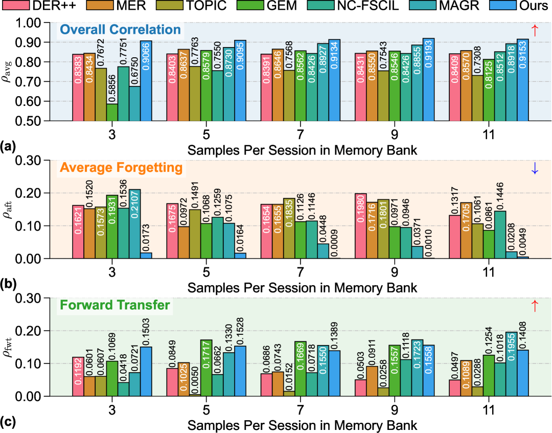
Figure 8: Comparison of different memory sizes on MTL-AQA.

Impact of Feature Supervision Layer. Fig. 9 investigates which layer of the I3D backbone should be layer-adaptive to balance stability and adaptability. Specifically, we aim to identify the boundary layer that yields optimal performance when used for feature supervision. Empirical results consistently point to the third layer as the most effective choice, which aligns with the outcomes of our dynamic layer selection strategy. This is reasonable since earlier layers mainly capture low-level visual patterns that are broadly transferable, while higher layers encode task-specific semantics that require adaptation. Thus, supervising features at the third layer provides an effective trade-off, preserving generalizable representations while allowing deeper layers to specialize.

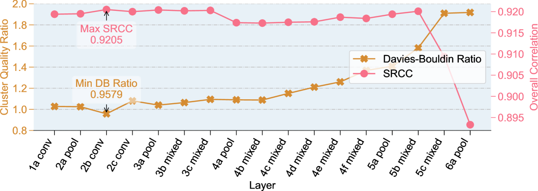
Figure 9: Cluster quality ratio and overall correlation.

Impact of Task Order. In practice, human skill progression is not strictly linear. To assess the impact of varying task sequences, we shuffled the task order multiple times and measured both performance and parameter changes (see Fig. 10). Our method shows strong robustness to task-order variation, achieving an average performance of $0.9183\pm 0.0028$, which is not only more stable but also higher than FS-Aug and NC-FSCIL. Moreover, in terms of parameter dynamics, our approach exhibits larger yet more structured parameter changes while maintaining higher performance and lower forgetting (see Fig. 10), highlighting its superior ability to manage catastrophic forgetting caused by parameter shifts.

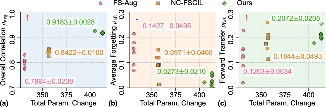
Figure 10: Performance vs. parameter changes across task orders.

Impact of Semi-Supervision and Noise. Fig. 11 evaluates MAGR++ under semi-supervised settings with limited labels (see Fig. 11) and in the presence of noisy annotations (see Fig. 11), two realistic and challenging issues in AQA that directly impact model generalization. Compared to MAGR, MAGR++ achieves consistently higher performance owing to its two-stage feature rectification and effective FPFT backbone tuning. With only 10 samples per session, MAGR++ reaches $\rho_{\text{avg}}=0.9162$ compared to MAGR’s 0.8741, and the margin remains at 25 samples (0.9256 vs. 0.8951). Under noise, MAGR++ is notably more resilient, sustaining 0.9234 at intensity 7 (see Fig. 11, $\hat{y}_{i}=0.94y_{i}+3.04$) while MAGR drops sharply to 0.7813 (see Fig. 11, $\hat{y}_{i}=0.65y_{i}+32.17$). Beyond MAGR, MAGR++ also outperforms other baselines: at 15 samples it achieves 0.9205 compared to 0.8950 for SLCA and 0.8142 for NC-FSCIL, and at noise level 7 it yields 0.9234 compared to 0.8032 for SLCA (see Fig. 11, $\hat{y}_{i}=0.53y_{i}+37.34$), 0.7548 for NC-FSCIL (see Fig. 11, $\hat{y}_{i}=0.73y_{i}+24.71$), while TOPIC lags further at 0.7049. These results verify the superior robustness of MAGR++ under both label scarcity and noisy supervision.

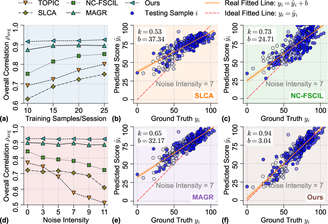
Figure 11: Performance comparison under label scarcity and labeling noise. 11 varies the number of training samples per session, and 11 evaluates robustness under noisy annotations. 11, 11, 11, and 11 show correlation plots at noise level 7, with fitted regression lines.

V-D Qualitative and Quantitative Results

We provide additional experimental results to further validate the effectiveness of our proposed method.

Flatness of Loss Landscape. To assess model generalization, we visualize the flatness of the loss landscape [58]. After training each session, model weights are perturbed along 10 random directions, and the resulting loss curves are averaged across perturbation magnitudes. Figs. 12, 12, 12, 12 and 12 illustrate session-wise results, while Fig. 12 shows the average over all five sessions. MAGR++ consistently exhibits flatter and lower loss landscapes than all other baselines, suggesting it converges to more stable minima that enhance generalization and mitigate catastrophic forgetting. In contrast, FS-Aug produces uneven and fluctuating curves, reflecting sensitivity to noise and a lack of robustness in its learned representations.

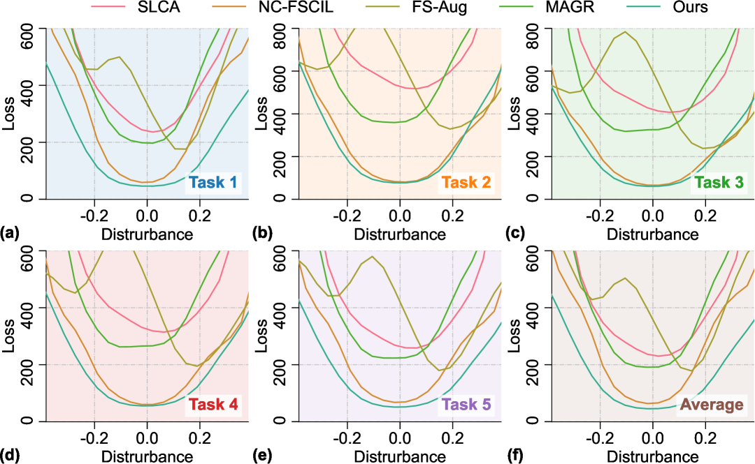
Figure 12: Loss landscapes on MTL-AQA. 12-12 show loss curves for five sessions, while 12 presents the average curve.

Visualization of Addressing Feature Shifts. To better understand catastrophic forgetting, we visualize feature distributions and scatter correlation in Fig. 13. In Figs. 13, 13, 13 and 13, MER exhibits severe manifold shifts where samples from different sessions are highly entangled, leading to a poorly aligned regression line $\hat{y}_{i}=0.11y_{i}+76.78$. FS-Aug and MAGR alleviate this overlap but still suffer from residual shifts, with regression lines remaining misaligned (e.g., MAGR: $\hat{y}_{i}=0.73y_{i}+23.90$ (see Fig. 13)). In contrast, our method explicitly separates samples across sessions (see Figs. 13, 13 and 13) and achieves a much closer regression fit $\hat{y}_{i}=0.90y_{i}+7.63$ (see Fig. 13), approaching the ideal line $\hat{y}_{i}=y_{i}$. These results indicate that our approach effectively mitigates feature shifts, preserving both feature space consistency and correlation accuracy across tasks.

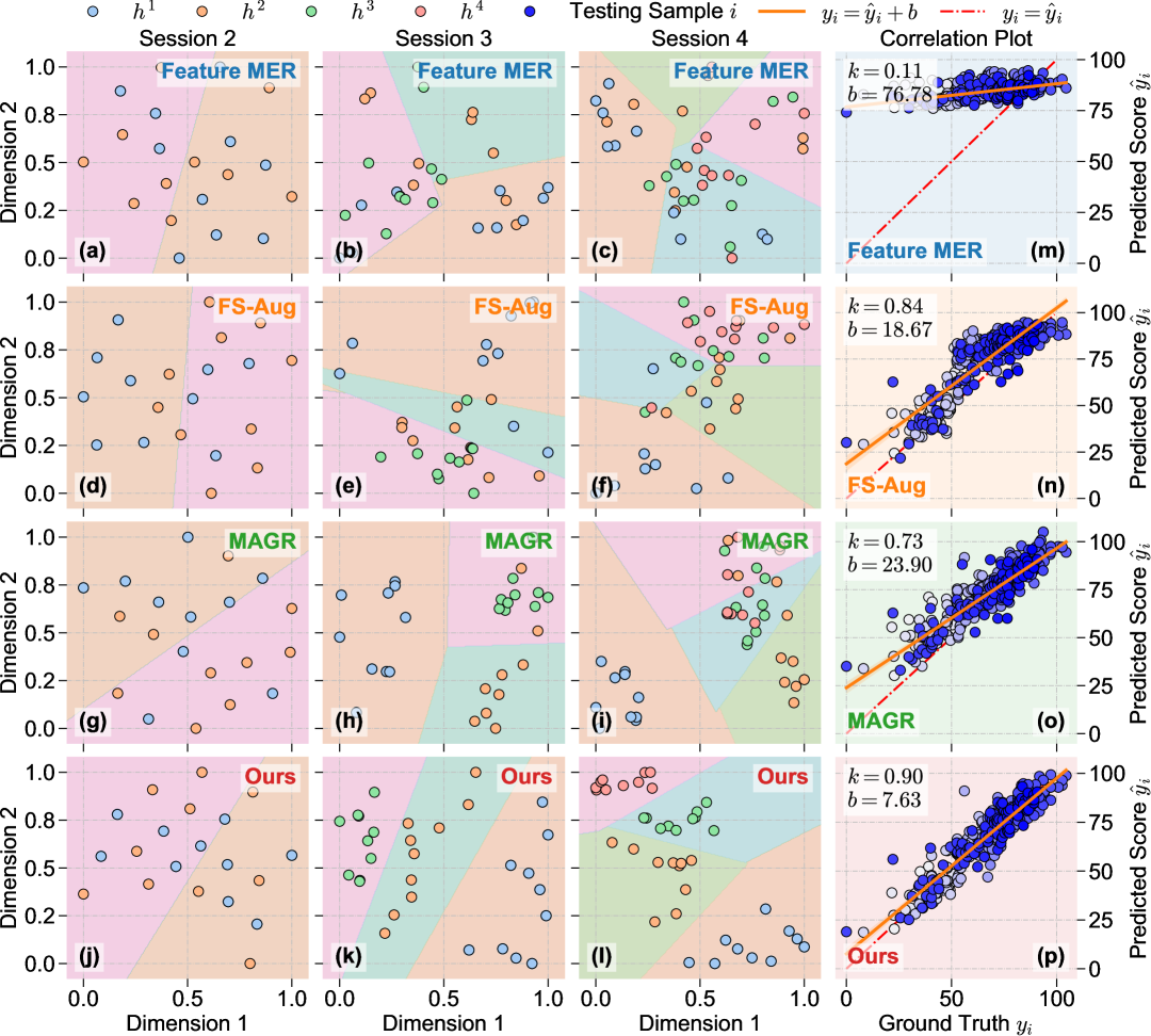
Figure 13: Visualization of t-SNE feature distributions (first three columns) and overall correlation plots (last column). The feature space is projected into two dimensions and normalized to $[0,1]$.

Error Analysis. Fig. 14 compares error distributions and cumulative accuracy among baselines and MAGR++. SLCA, FS-Aug, and MAGR achieve mean absolute errors of $10.80\pm 8.83$, $12.48\pm 8.41$, and $9.68\pm 6.17$, respectively. In contrast, MAGR++ significantly reduces the error to $5.26\pm 4.39$, indicating both lower bias and variance. The cumulative accuracy curves further emphasize this gain: MAGR++ reaches an AUC of $0.91$, surpassing SLCA ($0.81$), FS-Aug ($0.78$), and MAGR ($0.83$) by margins of $0.10$, $0.13$, and $0.08$, respectively. These results confirm the effectiveness of shift-aware rectification in improving both accuracy and stability for CAQA.

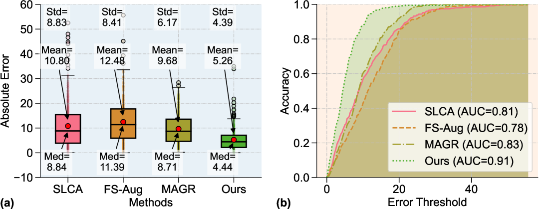
Figure 14: Error analysis on MTL-AQA. 14: Boxplots of absolute errors with mean, median, and standard deviation. 14: Cumulative error accuracy curves with area under the curve (AUC).

VI Discussion and Conclusion

In this work, we introduce the first formulation of CAQA, extending CL to fine-grained regression in AQA. To support this new paradigm, we construct four comprehensive benchmarks with tailored evaluation metrics and strong baselines, enabling fair cross-dataset comparison. Through an empirical study, we demonstrate that existing CL paradigms are insufficient for CAQA, and FPFT is necessary to bridge the gap between upstream action recognition and downstream fine-grained quality assessment. Our theoretical analysis further shows that FPFT is prone to overfitting during long-term adaptation and is vulnerable to manifold shift when replaying old features. To address these challenges, we proposed MAGR++, which integrates FPFT with layer-adaptive selection to stabilize continual updates, a manifold projector to rectify deviated features, and graph regularization to regulate feature space. Experiments show that MAGR++ consistently achieves state-of-the-art performance across various benchmarks. We believe this work establishes a solid foundation for future research on continual adaptation in fine-grained video understanding.

Despite these promising results, several avenues remain open. First, our current formulation focuses on CL of AQA tasks. Extending MAGR++ to more general CL scenarios could further validate its applicability. Second, integrating multi-modal inputs (e.g., audio and text) may improve the robustness and effectiveness. Third, incorporating online adaptation mechanisms could enhance efficiency for deployment in real-time settings. We view these directions as natural and impactful extensions toward advancing CAQA research.

Kanglei Zhou specializes in action quality assessment and continual learning. He is currently a Postdoctoral Researcher in the Department of Psychology and Cognitive Science at Tsinghua University. He received the Ph.D. degree in Computer Science and Engineering from Beihang University, Beijing, China. In 2024, he was a Visiting Student in the Department of Computer Science at Durham University, U.K. He obtained the B.E. degree from the College of Computer and Information Engineering, Henan Normal University, Xinxiang, China, in 2020.

Qingyi Pan is currently pursuing his Ph.D. degree at the Department of Statistics and Data Science at Tsinghua University. He received his M.S. degree from the Department of Computer Science and Technology at Tsinghua University in 2022. His research interest focuses on continual learning, interpretability, and uncertainty quantification for multivariate time series forecasting.

Xingxing Zhang received the BE and PhD degrees from the Institute of Information Science, Beijing Jiaotong University, in 2015 and 2020, respectively. She was also a visiting student with the Department of Computer Science, University of Rochester, from 2018 to 2019. She was a postdoc with the Department of Computer Science and Technology, Tsinghua University, from 2020 to 2022. Her research interests include continual learning and few-shot learning. She received the Excellent PhD Thesis Award from the Chinese Institute of Electronics in 2020.

Hubert P. H. Shum (Senior Member, IEEE) is a Professor of Visual Computing and the Director of Research for the Department of Computer Science at Durham University, specialising in modelling spatio-temporal information with responsible AI. He is also a Co-Founder and the Co-Director of Durham University Space Research Centre. He received his PhD degree from the University of Edinburgh. He chaired conferences such as Pacific Graphics, BMVC and SCA. He has authored over 200 research publications in the fields of Computer Vision, Computer Graphics and AI in Healthcare.

Frederick W. B. Li received a B.A. and an M.Phil. degree from Hong Kong Polytechnic University, and a Ph.D. degree from the City University of Hong Kong. He is currently an Associate Professor at Durham University, researching computer graphics, deep learning, collaborative virtual environments, and educational technologies. He is also an Associate Editor of Frontiers in Education and an Editorial Board Member of Virtual Reality & Intelligent Hardware. He chaired conferences such as ISVC and ICWL.

Xiaohui Liang (Member, IEEE) received his Ph.D. degree in computer science and engineering from Beihang University, China. He is currently a Professor, working in the School of Computer Science and Engineering at Beihang University. His main research interests include computer graphics and animation, visualization, and virtual reality.

Liyuan Wang is currently an Assistant Professor in the Department of Psychological and Cognitive Sciences at Tsinghua University. He received the B.S. and Ph.D. degrees from Tsinghua University, where he also conducted his postdoctoral research. He has an interdisciplinary background in neuroscience and machine learning. His work on continual learning has been published in major conferences and journals in related fields, such as Nature Machine Intelligence, TPAMI, TNNLS, NeurIPS, ICLR, CVPR, ICCV, ECCV, etc.

Appendix A Proof of Theorem 1

Proof 1

Let $\bm{v}:=\bm{\theta}-\bm{\theta}_{\text{up}}$ and $\mathcal{S}:=\mathrm{range}(\mathbf{U})$. Define the linearized risk

$$\widetilde{R}_{\text{down}}(\bm{v}):=\mathbb{E}_{(x,y)\sim\mathcal{D}_{\text{down}}}\,\ell\!\big(\phi_{\bm{\theta}_{\text{up}}}(x)+\mathbf{J}_{\text{up}}(x)^{\top}\bm{v},\,y\big),$$ (A13)

together with the $\mathbf{\Sigma}_{0}$-norm

$$\|\bm{w}\|_{\mathbf{\Sigma}_{0}}^{2}:=\bm{w}^{\top}\mathbf{\Sigma}_{0}\bm{w}.$$ (A14)

By Taylor’s theorem, for $\bm{v}^{\star}:=\arg\min_{\bm{v}}\widetilde{R}_{\text{down}}(\bm{v})$ and any $\bm{v}$ in the NTK neighborhood, one has

$$\widetilde{R}_{\text{down}}(\bm{v})\;\geq\;\widetilde{R}_{\text{down}}(\bm{v}^{\star})+\tfrac{1}{2}(\bm{v}-\bm{v}^{\star})^{\top}\mathbf{H}(\bm{v})(\bm{v}-\bm{v}^{\star}),$$ (A15)

where

$$\mathbf{H}(\bm{v})=\mathbb{E}_{(x,y)\sim\mathcal{D}_{\text{down}}}\!\big[\ell^{\prime\prime}(\phi_{\bm{\theta}_{\text{up}}}(x)+\mathbf{J}_{\text{up}}(x)^{\top}\bar{\bm{v}},y)\,\mathbf{J}_{\text{up}}(x)\mathbf{J}_{\text{up}}(x)^{\top}\big]\succeq\mu\,\mathbf{\Sigma}_{0}$$ (A16)

for some $\bar{\bm{v}}$ on the segment $[\bm{v}^{\star},\bm{v}]$. This implies

$$\widetilde{R}_{\text{down}}(\bm{v})-\widetilde{R}_{\text{down}}(\bm{v}^{\star})\;\geq\;\tfrac{\mu}{2}\,\|\bm{v}-\bm{v}^{\star}\|_{\mathbf{\Sigma}_{0}}^{2}.$$ (A17)

Since PEFT restricts $\bm{v}$ to $\mathcal{S}$, let $\bm{v}_{\mathcal{S}}:=\arg\min_{\bm{v}\in\mathcal{S}}\widetilde{R}_{\text{down}}(\bm{v})$. By Eq. A17, it follows that

$$\widetilde{R}_{\text{down}}(\bm{v}_{\mathcal{S}})-\widetilde{R}_{\text{down}}(\bm{v}^{\star})\;\geq\;\tfrac{\mu}{2}\,\inf_{\bm{s}\in\mathcal{S}}\|\bm{s}-\bm{v}^{\star}\|_{\mathbf{\Sigma}_{0}}^{2}=\tfrac{\mu}{2}\,\big\|\bm{v}^{\star}-\Pi_{\mathcal{S}}^{(\mathbf{\Sigma}_{0})}(\bm{v}^{\star})\big\|_{\mathbf{\Sigma}_{0}}^{2},$$ (A18)

where $\Pi_{\mathcal{S}}^{(\mathbf{\Sigma}_{0})}$ is the $\mathbf{\Sigma}_{0}$-orthogonal projection onto $\mathcal{S}$. Substituting $\bm{v}^{\star}=\bm{\theta}_{\text{down}}^{\star}-\bm{\theta}_{\text{up}}$ gives

$$\big\|\bm{v}^{\star}-\Pi_{\mathcal{S}}^{(\mathbf{\Sigma}_{0})}(\bm{v}^{\star})\big\|_{\mathbf{\Sigma}_{0}}=\big\|\Pi_{\mathcal{S}^{\perp}}^{(\mathbf{\Sigma}_{0})}(\bm{\theta}_{\text{down}}^{\star}-\bm{\theta}_{\text{up}})\big\|_{\mathbf{\Sigma}_{0}}.$$ (A19)

Finally, by assumption (A3), for $\|\bm{v}_{\mathcal{S}}\|,\|\bm{v}^{\star}\|\leq\rho$,

$$R_{\text{down}}(\bm{\theta}_{\text{up}}+\bm{v}_{\mathcal{S}})-R_{\text{down}}(\bm{\theta}_{\text{down}}^{\star})\;\geq\;\widetilde{R}_{\text{down}}(\bm{v}_{\mathcal{S}})-\widetilde{R}_{\text{down}}(\bm{v}^{\star})-\tfrac{L_{\varepsilon}}{2}\big(\|\bm{v}_{\mathcal{S}}\|^{2}+\|\bm{v}^{\star}\|^{2}\big).$$ (A20)

Combining Eqs. A18, A19 and A20 yields

$$R_{\text{down}}(\bm{\theta}_{\text{up}}+\bm{v}_{\mathcal{S}})-R_{\text{down}}(\bm{\theta}_{\text{down}}^{\star})\;\geq\;\tfrac{\mu}{2}\,\big\|\Pi_{\mathcal{S}^{\perp}}^{(\mathbf{\Sigma}_{0})}(\bm{\theta}_{\text{down}}^{\star}-\bm{\theta}_{\text{up}})\big\|_{\mathbf{\Sigma}_{0}}^{2}-C_{\varepsilon},$$ (A21)

where $C_{\varepsilon}:=\tfrac{L_{\varepsilon}}{2}(\|\bm{v}_{\mathcal{S}}\|^{2}+\|\bm{v}^{\star}\|^{2})$. This establishes Eq. 2.

1

Input : Sequential training sets $\{\mathcal{D}^{t}_{\text{train}}\}_{t=1}^{T}$, memory size $M$, backbone $f$, regressor $g$, projector $p$, threshold $\epsilon$

Output : Trained $(f^{T},g^{T},p^{T})$

2

3Init: Pretrain $f$ (e.g., I3D) and init $g,p$; $\mathcal{M}\leftarrow\varnothing$;

4 for $t\leftarrow 1$ to $T$ do

5   

   Copy previous backbone $f^{t-1}$ and freeze $f^{t-1}$ ;

    // copy previous backbone

    $L_{\text{opt}}\leftarrow$ LayerSelection ( $f^{t-1},\ f^{t},\mathcal{D}^{1}_{\text{train}},\ \epsilon$ );

    // see Sect. IV-B, invoke Algorithm 2

6   

   // Mini-batch training loop

7    while not converged do

8       Sample current batch $\mathcal{B}^{t}=\{(\mathbf{x}_{i}^{t},y_{i}^{t})\}_{i=1}^{b_{2}}\subset\mathcal{D}^{t}_{\text{train}}$;

       // Forward through current and previous backbones

9       $\bm{h}_{i}^{t,l}\leftarrow f^{t,l}(\mathbf{x}_{i}^{t})$,   $\bm{z}_{i}^{t,l}\leftarrow f^{t-1,l}(\mathbf{x}_{i}^{t})$ for all layers $l$;

10      

      $\hat{y}_{i}^{t}\leftarrow g(\bm{h}_{i}^{t,L})$;   $\mathcal{L}_{\text{D}}\leftarrow\frac{1}{b_{2}}\sum_{i}(\hat{y}_{i}^{t}-y_{i}^{t})^{2}$;

       // Current-task loss (Eq. (1))

11      

      // Training phase 1: layer-adaptive FPFT (Eq. (6))

12       $\mathcal{L}_{\text{tune}}\leftarrow\frac{1}{b_{2}}\sum_{i}\sum_{l<L_{\text{opt}}}\|\bm{h}_{i}^{t,l}-\bm{z}_{i}^{t,l}\|_{2}^{2}$;

13      

      // Training phase 2: projector learning (Eqs. (7), (8))

14       $\bm{z}_{i}^{t}\leftarrow\bm{z}_{i}^{t,L}$;    $\bm{\hat{h}}_{i}^{t}\leftarrow\bm{z}_{i}^{t}+p(\bm{z}_{i}^{t})$;   $\mathcal{L}_{\text{proj}}\leftarrow\frac{1}{b_{2}}\sum_{i}\|\bm{h}_{i}^{t,L}-\bm{\hat{h}}_{i}^{t}\|_{2}^{2}$;

15      

16      Sample old feature batch $\tilde{\mathcal{B}}=\{(\tilde{\bm{h}}_{j},y_{j})\}_{j=1}^{b_{1}}\subset\mathcal{M}$;

17       foreach $(\tilde{\bm{h}}_{j},y_{j})\in\tilde{\mathcal{B}}$ do

          $\tilde{\bm{h}}_{j}\leftarrow\tilde{\bm{h}}_{j}+p(\tilde{\bm{h}}_{j})$ ;

          // deviated feature translation

18         

19      

      // Training phase 3: build joint batch and compute regularizer (Eq. (11))

20       $\mathbf{H}\leftarrow[\tilde{\bm{h}}_{1:b_{1}},\ \bm{h}^{t,L}_{1:b_{2}}]$;   $\bm{y}\leftarrow[y_{1:b_{1}},\ y^{t}_{1:b_{2}}]$;

       $\mathcal{L}_{\text{reg}}\leftarrow$ IIJGRLoss ( $\mathbf{H},\bm{y}$ );

       // angular distances + matrix partitions, see Eq. 11

21      

      $\hat{y}_{j}\leftarrow g(\tilde{\bm{h}}_{j})$;   $\mathcal{L}_{\text{M}}\leftarrow\frac{1}{b_{1}}\sum_{j}(\hat{y}_{j}-y_{j})^{2}$;

       // replay loss (Eq. (1))

22      

23      Update $\{f,g,p\}$ by backprop on $\mathcal{L}$ (optimizer, LR schedule, etc.);

24      

25   

   // End-of-session memory maintenance

26    foreach $(\tilde{\bm{h}},y)\in\mathcal{M}$ do

       $\tilde{\bm{h}}\leftarrow\tilde{\bm{h}}+p(\tilde{\bm{h}})$ ;

       // refresh old features via converged projector

27      

   $\mathcal{P}^{t}\leftarrow\textnormal{{OUS}}(\mathcal{D}^{t}_{\text{train}},f,g,M)$ ;

    // select new prototypes, invoke Algorithm 3

28    Update memory as $\mathcal{M}\leftarrow\mathcal{M}\cup\mathcal{P}^{t}$ and keep at most $M$ items;

29   

Algorithm 1 Training procedure of MAGR++ for CAQA

Appendix B Proof of Theorem 2

Proof 2

Let the per-session update be defined as

$$\bm{\Delta}_{t}:=\bm{\theta}^{t}-\bm{\theta}^{t-1},\qquad\Delta_{t}:=\|\bm{\Delta}_{t}\|.$$ (A22)

Define the per-task risk and its empirical counterpart as

$$R_{k}(\bm{\theta}):=\mathbb{E}_{(x,y)\sim\mathcal{D}_{k}}\,\ell\!\big(\phi_{\bm{\theta}}(x),y\big),\qquad\hat{R}_{k}(\bm{\theta}):=\mathbb{E}_{(x,y)\sim\text{mem}(k)}\,\ell\!\big(\phi_{\bm{\theta}}(x),y\big).$$ (A23)

At session $t$, define the stale and ideal replay objectives:

$$\mathcal{L}_{t}^{\text{stale}}(\bm{\theta}) =\mathbb{E}_{(x,y)\sim\mathcal{M}_{t-1}}\,\ell\!\big(g_{\bm{\theta}_{g}}(f_{\bm{\theta}_{f}^{t-1}}(x)),y\big),$$ (A24)

$$\mathcal{L}_{t}^{\text{ideal}}(\bm{\theta}) =\mathbb{E}_{(x,y)\sim\mathcal{M}_{t-1}}\,\ell\!\big(g_{\bm{\theta}_{g}}(f_{\bm{\theta}_{f}}(x)),y\big).$$

By Assumptions (B1) and (B2), evaluating at $\bm{\theta}=\bm{\theta}^{t}$ yields

$$\Big|\mathcal{L}_{t}^{\text{stale}}(\bm{\theta}^{t})-\mathcal{L}_{t}^{\text{ideal}}(\bm{\theta}^{t})\Big| \leq\mathbb{E}\,\big\|g_{\bm{\theta}_{g}^{t}}\!\big(f_{\bm{\theta}_{f}^{t-1}}(x)\big)-g_{\bm{\theta}_{g}^{t}}\!\big(f_{\bm{\theta}_{f}^{t}}(x)\big)\big\|$$ (A25)

$$\leq L_{g}\,\mathbb{E}\,\big\|f_{\bm{\theta}_{f}^{t-1}}(x)-f_{\bm{\theta}_{f}^{t}}(x)\big\|.$$

Using Assumption (B3) with $\|\bm{\theta}_{f}^{t}-\bm{\theta}_{f}^{t-1}\|=\Delta_{t}$, we have

$$\Big|\mathcal{L}_{t}^{\text{stale}}(\bm{\theta}^{t})-\mathcal{L}_{t}^{\text{ideal}}(\bm{\theta}^{t})\Big|\;\leq\;L_{g}\,L_{f}\,\Delta_{t}.$$ (A26)

If there exists a projector $\mathbf{P}_{t}$ such that

$$\mathbb{E}\,\big\|f_{\bm{\theta}_{f}^{t}}(x)-\mathbf{P}_{t}f_{\bm{\theta}_{f}^{t-1}}(x)\big\|\leq\varepsilon_{t},$$ (A27)

the bound refines to

$$\Big|\mathcal{L}_{t}^{\text{stale}}(\bm{\theta}^{t})-\mathcal{L}_{t}^{\text{ideal}}(\bm{\theta}^{t})\Big|\;\leq\;L_{g}\,\varepsilon_{t}.$$ (A28)

Let $\mathcal{H}_{t-1}$ denote the model class realizable near $\bm{\theta}^{t-1}$, and define

$$\mathcal{H}_{t}:=\mathcal{H}_{t-1}\cup\big\{\phi_{\bm{\theta}}:\|\bm{\theta}-\bm{\theta}^{t-1}\|\leq\Delta_{t}\big\}.$$ (A29)

By Assumption (B4), enlarging the parameter ball by $\Delta_{t}$ increases localized complexity (e.g., Rademacher or covering bounds) by at most $C_{0}L_{\phi}\Delta_{t}$, giving

$$\mathbb{E}\big[R_{k}(\bm{\theta}^{t})-\hat{R}_{k}(\bm{\theta}^{t})\big]\;\leq\;\mathbb{E}\big[R_{k}(\bm{\theta}^{t-1})-\hat{R}_{k}(\bm{\theta}^{t-1})\big]\;+\;C\,L_{\phi}\,\Delta_{t},$$ (A30)

for some constant $C>0$.

Define the forgetting as

$$\psi_{t}(k):=R_{k}(\bm{\theta}^{t})-R_{k}(\bm{\theta}^{t-1}).$$ (A31)

Adding and subtracting empirical risks gives

$$\psi_{t}(k)=\underbrace{R_{k}(\bm{\theta}^{t})-\hat{R}_{k}(\bm{\theta}^{t})}_{\text{(I)}}+\underbrace{\hat{R}_{k}(\bm{\theta}^{t})-\hat{R}_{k}(\bm{\theta}^{t-1})}_{\text{(II)}}+\underbrace{\hat{R}_{k}(\bm{\theta}^{t-1})-R_{k}(\bm{\theta}^{t-1})}_{\text{(III)}}.$$ (A32)

Taking expectations and applying Eq. A30 to (I) and (III) gives

$$\mathbb{E}[\text{(I)}+\text{(III)}]\;\lesssim\;C\,L_{\phi}\,\Delta_{t}.$$ (A33)

For (II), the empirical change is bounded by the stale–ideal gap plus the session-$t$ optimization suboptimality:

$$\mathbb{E}\big[\hat{R}_{k}(\bm{\theta}^{t})-\hat{R}_{k}(\bm{\theta}^{t-1})\big]\;\lesssim\;\Big|\mathcal{L}_{t}^{\text{stale}}(\bm{\theta}^{t})-\mathcal{L}_{t}^{\text{ideal}}(\bm{\theta}^{t})\Big|\;+\;E_{\text{opt}}.$$ (A34)

Combining Eqs. A26, A33 and A34 yields

$$\mathbb{E}[\psi_{t}(k)]\;\lesssim\;L_{g}L_{f}\,\Delta_{t}\;+\;C\,L_{\phi}\,\Delta_{t}\;+\;E_{\text{opt}},$$ (A35)

matching the bound in Eq. 3. In the projector case Eq. A27, replace $L_{g}L_{f}\Delta_{t}$ by $L_{g}\varepsilon_{t}$ from Eq. A28, completing the proof.

Appendix C Training Procedure

At each session $t$, MAGR++ jointly optimizes the backbone, regressor, and projector under the composite objective in Eq. 4. The training begins with Ordered Uniform Sampling (OUS) to store representative features from session $t{-}1$ in the memory bank $\mathcal{M}$, ensuring efficient replay coverage as required by the CAQA loss in Eq. 1. The backbone $f^{t}$ is then adapted to current data $\mathcal{D}^{t}_{\text{train}}$ via layer-adaptive FPFT, where shallow layers below $L_{\text{opt}}$ are constrained by the feature-matching loss in Eq. 6, while deeper layers are fully fine-tuned to capture evolving quality cues. To handle manifold shift, the Manifold Projector (MP) is trained using the projection loss in Eq. 8, aligning $f^{t-1}$ and $f^{t}$ representations with only current-session inputs, and subsequently applied to translate old features from $\mathcal{M}$ into the updated space for replay. In parallel, the Intra-Inter-Joint Graph Regularizer (IIJ-GR) minimizes the regularization loss in Eq. 11, enforcing both intra- and inter-session consistency between feature geometry and quality scores. Finally, the regressor $g^{t}$ is optimized on a mixture of rectified old features and current-session features, and the memory bank is refreshed by updating old features through MP and adding new prototypes. This coordinated pipeline ensures that MAGR++ balances adaptation and stability across sessions, while mitigating forgetting through replay. The details of the training procedure are shown in Algorithm 1.

Input: Base-session set $\mathcal{D}^{0}$, backbone $f$, threshold $\epsilon$

Output: Optimal boundary $L_{\text{opt}}$

1

2for $l\leftarrow 1$ to $L$ do

3    $\mathbf{Z}^{l}_{\text{fix}}\leftarrow f_{\text{fix}}^{l}(\mathcal{D}^{0})$;    $\mathbf{Z}^{l}_{\text{tune}}\leftarrow f_{\text{tune}}^{l}(\mathcal{D}^{0})$;

4   

5   $r^{l}\leftarrow\mathcal{C}(\mathbf{Z}^{l}_{\text{tune}})/\mathcal{C}(\mathbf{Z}^{l}_{\text{fix}})$;

6   

7   if $r^{l}>1+\epsilon$ then

8       $L_{\text{opt}}\leftarrow l$;

9      

10   

return $L_{\text{opt}}$

Algorithm 2 LayerSelection: Layer Selection

Input: Training set $\mathcal{D}^{t}$, memory size $M$, scorer $g$

Output: Prototype set $\mathcal{P}^{t}$

1

2Compute scores $y_{i}=g^{t}(f^{t}(\mathbf{x}_{i}))$ for all $\mathbf{x}_{i}\in\mathcal{D}^{t}$;

3 Sort $\mathcal{D}^{t}$ by $y_{i}$ in ascending order;

4 Divide sorted samples into $M$ intervals uniformly across score range;

5 Select one representative sample from each interval;

return $\mathcal{P}^{t}$

Algorithm 3 OUS: Ordered Uniform Sampling

TABLE A6: Experiments on UNLV-Vault.

a UNLV-Vault (offline)

Method	Publisher	Memory	$\rho_{\text{avg}}$ ($\uparrow$)	$\rho_{\text{aft}}$ ($\downarrow$)	$\rho_{\text{fwt}}$ ($\uparrow$)
Joint Training (UB)	-	None	$0.7514$	-	-
Sequential FT (LB)	-	None	$0.5168$	0.1887	$0.3445$
SI [41]	ICML’17	None	$0.5165$	0.2287	$0.2839$
EWC [42]	PNAS’17	None	$0.5173$	0.2250	$0.2371$
LwF [43]	TPAMI’17	None	$0.6659$	0.1371	$0.4318$
MER [44]	ICLR’19	Raw Data	$0.5883$	0.1458	$0.4053$
DER++ [45]	NeurIPS’20	Raw Data	$0.5905$	0.3693	$0.2150$
TOPIC [46]	CVPR’20	Raw Data	$0.5429$	0.1712	$0.3183$
GEM [47]	ICCV’21	Raw Data	$0.5339$	0.1854	$0.0608$
Feature MER	-	Feature	$0.4342$	0.1856	$0.4578$
SLCA [48]	ICCV’23	Feature	$0.4919$	0.1221	$0.3972$
NC-FSCIL [50]	ICLR’23	Feature	$0.5747$	0.2664	$0.4863$
FS-Aug [39]	TCSVT’24	Feature	$0.5146$	0.2113	$0.4275$
MAGR [22]	ECCV’24	Feature	$0.6526$	0.0687	$0.2853$
MAGR++ (Ours)	-	Feature	$0.7012$	0.2425	$0.2534$

b UNLV-Vault (online)

Method	Publisher	Memory	$\rho_{\text{avg}}$ ($\uparrow$)	$\rho_{\text{aft}}$ ($\downarrow$)	$\rho_{\text{fwt}}$ ($\uparrow$)
Sequential FT (LB)	-	None	$0.2139$	0.0684	$0.5507$
SI [41]	ICML’17	None	$-0.2904$	0.0897	$0.2912$
EWC [42]	PNAS’17	None	$0.0585$	0.0385	$0.2288$
LwF [43]	TPAMI’17	None	$-0.1075$	0.2311	$0.1540$
MER [44]	ICLR’19	Raw Data	$0.0441$	0.2533	$0.2597$
DER++ [45]	NeurIPS’20	Raw Data	$-0.1701$	0.1642	$0.2853$
TOPIC [46]	CVPR’20	Raw Data	$0.0590$	0.1013	$0.3340$
GEM [47]	ICCV’21	Raw Data	$0.0391$	0.1013	$0.3340$
Feature MER	-	Feature	$0.3571$	0.1444	$-0.0213$
SLCA [48]	ICCV’23	Feature	$0.0962$	0.1242	$0.2670$
NC-FSCIL [50]	ICLR’23	Feature	$0.4971$	0.0291	$-0.0463$
FS-Aug [39]	TCSVT’24	Feature	$0.1998$	0.1350	$0.1497$
MAGR [22]	ECCV’24	Feature	$0.1986$	0.1201	$-0.1483$
MAGR++ (Ours)	-	Feature	$0.5806$	0.0000	$0.7057$

Figure A15: Representative samples from MTL-AQA covering high-, mid-, and low-score cases. The first five columns show sampled frames, and the last column reports assessment results with errors. A15 and A15 show successful cases, while A15 depicts a failure case.

Appendix D Additional Experiments

D-A Experimental Setting

UNLV-Vault. To further verify the generalization of our method beyond diving, we include the UNLV-Vault dataset in our evaluations. UNLV-Vault contains 176 gymnastics vault videos is treated as the “vault” class in the AQA-7 benchmark [30]. Each video sequence is sampled to 103 frames, covering the complete vault motion from run-up to landing. Each sample is annotated by expert judges under the standard vault scoring system. In our experiments, we follow the same split as in prior works (120 for training and 56 for testing). Since vault actions differ substantially from diving, with shorter durations, more abrupt motions, and distinct visual cues, this dataset serves as a complementary testbed to assess whether our method can maintain performance under domain shift. The results show that MAGR++ retains strong performance on UNLV-Vault, supporting its generalization across different action domains.

TABLE A7: Additional ablation results on MTL-AQA. Reported percentages denote relative changes compared to ID 1.

ID	Setting	$\rho_{\text{avg}}$ ($\uparrow$)	$\rho_{\text{aft}}$ ($\downarrow$)	$\rho_{\text{fwt}}$ ($\uparrow$)
1	MAGR++ (Ours)	0.9205	0.0103	0.1274
2	MP w/o Residual Link	0.8933-3%	0.0389+278%	0.0693-46%
3	Eq. 11 w/ KL Loss	0.9173-0.3%	0.0155+51%	0.1029-19%

D-B Results and Analysis

Generalization to Other Domains Beyond Diving. To further verify the cross-domain robustness of our approach, we evaluate MAGR++ on the UNLV-Vault dataset, which differs significantly from diving in terms of motion dynamics and temporal structure. As summarized in Tab. A6, MAGR++ achieves the best overall performance in both offline and online settings. In the offline case, it attains $\rho_{\text{avg}}=0.7012$, outperforming the strongest baseline MAGR [22] by $+0.0486$, NC-FSCIL [50] by $+0.1265$, and SLCA [48] by $+0.2093$. In the online setting, MAGR++ reaches $\rho_{\text{avg}}=0.5806$, yielding a substantial improvement of $+0.0835$ over NC-FSCIL (0.4971) and $+0.3810$ over FS-Aug (0.1998). It also maintains zero forgetting ($\rho_{\text{aft}}=0$) and the highest forward transfer ($\rho_{\text{fwt}}=0.7057$), indicating strong adaptability without sacrificing stability. These results demonstrate that the proposed layer-adaptive fine-tuning and two-step rectification effectively preserve feature–score alignment even when transferred to unseen domains with distinct motion and visual characteristics.

Ablation Study. As shown in Tab. A7, removing the residual link in MP leads to a notable decline in performance, with the average correlation dropping by about 3%, the after-effect increasing nearly threefold, and the forward transfer reduced by almost half. This observation highlights that the residual connection is essential for capturing substantial feature variations and maintaining stability across continual updates. In contrast, substituting the MSE term in Eq. 11 with a KL divergence yields only marginal changes, demonstrating that our method remains robust regardless of the specific feature-matching loss. Overall, these results confirm the stability and robustness of MAGR++, showing that its performance is largely insensitive to minor design variations, yet heavily reliant on the residual link for effective adaptation.

Case Study. Fig. A15 illustrates representative samples from the MTL-AQA dataset, covering low-, high-, and mid-score diving scenarios. We further compare the predictions of different methods, including SLCA [48], NC-FSCIL [50], FS-Aug [39], MAGR [22], and our approach. Fig. A15 illustrates representative samples from the MTL-AQA dataset, covering low-, high-, and mid-score diving scenarios, with predictions compared across SLCA [48], NC-FSCIL [50], FS-Aug [39], MAGR [22], and our approach. In the low-score case (Sample #006), the dive produces a large splash indicating poor execution, where the ground-truth score is 25.65 and our method predicts 26.03 with only 0.38 error, while SLCA (59.75, error 34.10) and FS-Aug (36.71, error 11.06) perform much worse. In the high-score case (Sample #138), the nearly splash-free entry yields a ground truth of 90.75, and our method achieves 90.54 with 0.21 error, whereas NC-FSCIL (100.34, error 9.59) and SLCA (82.58, error 7.77) deviate substantially. Even in the more challenging mid-score case (Sample #021), where the ground truth is 52.70, our method outputs 66.43, closer to the target than NC-FSCIL (70.43) and SLCA (69.44). These examples highlight the superior reliability of our method across both extreme and intermediate performance levels. At the same time, they reveal common error modes: occlusions (e.g., body–water overlap) may lead to misaligned features, while abrupt motion changes can induce projection failures, which explains the remaining discrepancies. Analyzing such cases not only clarifies why errors occur but also highlights promising directions for future research, such as developing representations that are intrinsically robust to occlusion and designing projection mechanisms that explicitly account for dynamic motion patterns.

Appendix E Additional Discussion and Future Work

While MAGR++ demonstrates strong performance and generalization across diverse CAQA benchmarks, several open challenges remain. First, although the proposed layer-adaptive fine-tuning effectively balances stability and adaptability, it relies on clustering-based abstraction estimation. Future work could explore more efficient or theoretically grounded criteria, such as information-theoretic or gradient-based layer importance measures. Second, MP is currently implemented as a simple MLP, which assumes local smoothness in feature transitions. Incorporating spatiotemporal attention or motion-conditioned projection could better handle complex distribution shifts caused by abrupt dynamics or occlusions. Third, while our two-step rectification preserves feature–score alignment, it primarily focuses on visual modality. Extending this framework to multi-modal settings (e.g., integrating pose or textual feedback) would further enhance interpretability and robustness. Finally, although our evaluations cover multiple datasets and both offline and online CAQA settings, future studies could examine real-time deployment and memory-limited environments to further assess scalability and practicality. Overall, we envision MAGR++ as a foundation for building trustworthy, adaptive AQA systems capable of CL under realistic scenarios.

References

- [1] K. Gedamu, Y. Ji, Y. Yang, J. Shao, and H. T. Shen, “Self-supervised subaction parsing network for semi-supervised action quality assessment,” IEEE Transactions on Image Processing, 2024.
- [2] A. Majeedi, V. R. Gajjala, S. S. S. N. GNVV, and Y. Li, “Rica2: Rubric-informed, calibrated assessment of actions,” in European Conference on Computer Vision, vol. 15121, pp. 143–161, 2024.
- [3] X. Dong, X. Liu, W. Li, A. Adeyemi-Ejeye, and A. Gilbert, “Interpretable long-term action quality assessment,” arXiv preprint arXiv:2408.11687, 2024.
- [4] J. Liu, H. Wang, W. Zhou, K. Stawarz, P. Corcoran, Y. Chen, and H. Liu, “Adaptive spatiotemporal graph transformer network for action quality assessment,” IEEE Transactions on Circuits and Systems for Video Technology, 2025.
- [5] L.-A. Zeng and W.-S. Zheng, “Multimodal action quality assessment,” IEEE Transactions on Image Processing, vol. 33, pp. 1600–1613, 2024.
- [6] Y. Ji, L. Ye, H. Huang, L. Mao, Y. Zhou, and L. Gao, “Localization-assisted uncertainty score disentanglement network for action quality assessment,” in ACM International Conference on Multimedia, pp. 8590–8597, 2023.
- [7] S. Zhang, W. Dai, S. Wang, X. Shen, J. Lu, J. Zhou, and Y. Tang, “Logo: A long-form video dataset for group action quality assessment,” in IEEE/CVF Conference on Computer Vision and Pattern Recognition, pp. 2405–2414, 2023.
- [8] K. Zhou, R. Cai, Y. Ma, Q. Tan, X. Wang, J. Li, H. P. Shum, F. W. Li, S. Jin, and X. Liang, “A video-based augmented reality system for human-in-the-loop muscle strength assessment of juvenile dermatomyositis,” IEEE Transactions on Visualization and Computer Graphics, vol. 29, no. 5, pp. 2456–2466, 2023.
- [9] P. Parmar, J. Reddy, and B. Morris, “Piano skills assessment,” in 2021 IEEE 23rd International Workshop on Multimedia Signal Processing (MMSP), pp. 1–5, IEEE, 2021.
- [10] Z. Li, L. Gu, W. Wang, R. Nakamura, and Y. Sato, “Surgical skill assessment via video semantic aggregation,” in International Conference on Medical Image Computing and Computer-Assisted Intervention, pp. 410–420, Springer, 2022.
- [11] J. Carreira and A. Zisserman, “Quo vadis, action recognition? a new model and the kinetics dataset,” in IEEE/CVF Conference on Computer Vision and Pattern Recognition, pp. 6299–6308, 2017.
- [12] W. Kay, J. Carreira, K. Simonyan, B. Zhang, C. Hillier, S. Vijayanarasimhan, F. Viola, T. Green, T. Back, P. Natsev, et al., “The kinetics human action video dataset,” arXiv preprint arXiv:1705.06950, 2017.
- [13] L. Wang, X. Zhang, H. Su, and J. Zhu, “A comprehensive survey of continual learning: Theory, method and application,” IEEE Transactions on Pattern Analysis and Machine Intelligence, 2024.
- [14] Z. Chi, L. Gu, H. Liu, Y. Wang, Y. Yu, and J. Tang, “Metafscil: A meta-learning approach for few-shot class incremental learning,” in IEEE/CVF Conference on Computer Vision and Pattern Recognition, pp. 14166–14175, 2022.
- [15] L. Wang, J. Xie, X. Zhang, M. Huang, H. Su, and J. Zhu, “Hierarchical decomposition of prompt-based continual learning: Rethinking obscured sub-optimality,” Advances in Neural Information Processing Systems, vol. 36, 2024.
- [16] L. Wang, M. Zhang, Z. Jia, Q. Li, C. Bao, K. Ma, J. Zhu, and Y. Zhong, “Afec: Active forgetting of negative transfer in continual learning,” Advances in Neural Information Processing Systems, vol. 34, pp. 22379–22391, 2021.
- [17] K. Zhou, Z. Hao, L. Wang, and X. Liang, “Adaptive score alignment learning for continual perceptual quality assessment of 360-degree videos in virtual reality,” IEEE Transactions on Visualization and Computer Graphics, 2025.
- [18] Y. Xin, J. Yang, S. Luo, H. Zhou, J. Du, X. Liu, Y. Fan, Q. Li, and Y. Du, “Parameter-efficient fine-tuning for pre-trained vision models: A survey,” arXiv preprint arXiv:2402.02242, 2024.
- [19] K. Zhou, R. Cai, L. Wang, H. P. H. Shum, and X. Liang, “A comprehensive survey of action quality assessment: Method and benchmark,” arXiv preprint arXiv:2412.11149, 2024.
- [20] K. Zhou, J. Li, R. Cai, L. Wang, X. Zhang, and X. Liang, “Cofinal: Enhancing action quality assessment with coarse-to-fine instruction alignment,” in International Joint Conference on Artificial Intelligence, pp. 1771–1779, 2024.
- [21] K. Zhou, H. P. Shum, F. W. Li, X. Zhang, and X. Liang, “Phi: Bridging domain shift in long-term action quality assessment via progressive hierarchical instruction,” IEEE Transactions on Image Processing, vol. 34, pp. 3718–3732, 2025.
- [22] K. Zhou, L. Wang, X. Zhang, H. P. Shum, F. W. Li, J. Li, and X. Liang, “Magr: Manifold-aligned graph regularization for continual action quality assessment,” in European Conference on Computer Vision, pp. 375–392, 2024.
- [23] J. Xu, Y. Rao, X. Yu, G. Chen, J. Zhou, and J. Lu, “Finediving: A fine-grained dataset for procedure-aware action quality assessment,” in IEEE/CVF Conference on Computer Vision and Pattern Recognition, pp. 2949–2958, 2022.
- [24] P. Parmar and B. Morris, “Action quality assessment across multiple actions,” in WACV, pp. 1468–1476, IEEE, 2019.
- [25] H. Pirsiavash, C. Vondrick, and A. Torralba, “Assessing the quality of actions,” in European Conference on Computer Vision, pp. 556–571, Springer, 2014.
- [26] H. Xu, H. Wu, X. Ke, Y. Li, R. Xu, and W. Guo, “Quality-guided vision-language learning for long-term action quality assessment,” IEEE Transactions on Multimedia, 2025.
- [27] H. Xu, X. Ke, Y. Li, R. Xu, H. Wu, X. Lin, and W. Guo, “Vision-language action knowledge learning for semantic-aware action quality assessment,” in European Conference on Computer Vision, 2024.
- [28] A. Zia, Y. Sharma, V. Bettadapura, E. L. Sarin, T. Ploetz, M. A. Clements, and I. Essa, “Automated video-based assessment of surgical skills for training and evaluation in medical schools,” International Journal of Computer Assisted Radiology and Surgery, vol. 11, pp. 1623–1636, 2016.
- [29] J.-H. Pan, J. Gao, and W.-S. Zheng, “Adaptive action assessment,” IEEE Transactions on Pattern Analysis and Machine Intelligence, vol. 44, no. 12, pp. 8779–8795, 2021.
- [30] X. Yu, Y. Rao, W. Zhao, J. Lu, and J. Zhou, “Group-aware contrastive regression for action quality assessment,” in IEEE/CVF International Conference on Computer Vision, pp. 7919–7928, 2021.
- [31] P. Parmar and B. T. Morris, “What and how well you performed? a multitask learning approach to action quality assessment,” in IEEE/CVF Conference on Computer Vision and Pattern Recognition, pp. 304–313, 2019.
- [32] K. Zhou, Y. Ma, H. P. Shum, and X. Liang, “Hierarchical graph convolutional networks for action quality assessment,” IEEE Transactions on Circuits and Systems for Video Technology, vol. 33, no. 12, pp. 7749–7763, 2023.
- [33] X. Ke, H. Xu, X. Lin, and W. Guo, “Two-path target-aware contrastive regression for action quality assessment,” Information Sciences, vol. 664, p. 120347, 2024.
- [34] H. Doughty, W. Mayol-Cuevas, and D. Damen, “The pros and cons: Rank-aware temporal attention for skill determination in long videos,” in IEEE/CVF Conference on Computer Vision and Pattern Recognition, pp. 7862–7871, 2019.
- [35] H. Doughty, D. Damen, and W. Mayol-Cuevas, “Who’s better? who’s best? pairwise deep ranking for skill determination,” in IEEE/CVF Conference on Computer Vision and Pattern Recognition, pp. 6057–6066, 2018.
- [36] A. Dadashzadeh, S. Duan, A. Whone, and M. Mirmehdi, “Pecop: Parameter efficient continual pretraining for action quality assessment,” in WACV, pp. 42–52, 2024.
- [37] J. Xu, S. Yin, G. Zhao, Z. Wang, and Y. Peng, “Fineparser: A fine-grained spatio-temporal action parser for human-centric action quality assessment,” in IEEE/CVF Conference on Computer Vision and Pattern Recognition, pp. 14628–14637, 2024.
- [38] J. Xu, S. Yin, and Y. Peng, “Human-centric fine-grained action quality assessment,” IEEE Transactions on Pattern Analysis and Machine Intelligence, 2025.
- [39] Y.-M. Li, L.-A. Zeng, J.-K. Meng, and W.-S. Zheng, “Continual action assessment via task-consistent score-discriminative feature distribution modeling,” IEEE Transactions on Circuits and Systems for Video Technology, 2024.
- [40] L. Wang, X. Zhang, Q. Li, M. Zhang, H. Su, J. Zhu, and Y. Zhong, “Incorporating neuro-inspired adaptability for continual learning in artificial intelligence,” Nature Machine Intelligence, vol. 5, no. 12, pp. 1356–1368, 2023.
- [41] F. Zenke, B. Poole, and S. Ganguli, “Continual learning through synaptic intelligence,” in International Conference on Machine Learning, pp. 3987–3995, PMLR, 2017.
- [42] J. Kirkpatrick, R. Pascanu, N. Rabinowitz, J. Veness, G. Desjardins, A. A. Rusu, K. Milan, J. Quan, T. Ramalho, A. Grabska-Barwinska, D. Hassabis, C. Clopath, D. Kumaran, and R. Hadsell, “Overcoming catastrophic forgetting in neural networks,” Proceedings of the National Academy of Sciences, vol. 114, no. 13, pp. 3521–3526, 2017.
- [43] Z. Li and D. Hoiem, “Learning without forgetting,” IEEE Transactions on Pattern Analysis and Machine Intelligence, vol. 40, no. 12, pp. 2935–2947, 2017.
- [44] M. Riemer, I. Cases, R. Ajemian, M. Liu, I. Rish, Y. Tu, and G. Tesauro, “Learning to learn without forgetting by maximizing transfer and minimizing interference,” in International Conference on Learning Representations, 2019.
- [45] P. Buzzega, M. Boschini, A. Porrello, D. Abati, and S. Calderara, “Dark experience for general continual learning: A strong, simple baseline,” Advances in Neural Information Processing Systems, vol. 33, pp. 15920–15930, 2020.
- [46] X. Tao, X. Hong, X. Chang, S. Dong, X. Wei, and Y. Gong, “Few-shot class-incremental learning,” in IEEE/CVF Conference on Computer Vision and Pattern Recognition, pp. 12183–12192, 2020.
- [47] A. Kukleva, H. Kuehne, and B. Schiele, “Generalized and incremental few-shot learning by explicit learning and calibration without forgetting,” in IEEE/CVF International Conference on Computer Vision, pp. 9020–9029, 2021.
- [48] G. Zhang, L. Wang, G. Kang, L. Chen, and Y. Wei, “Slca: Slow learner with classifier alignment for continual learning on a pre-trained model,” IEEE/CVF International Conference on Computer Vision, pp. 19148–19158, 2023.
- [49] G. Zhang, L. Wang, G. Kang, L. Chen, and Y. Wei, “Slca++: Unleash the power of sequential fine-tuning for continual learning with pre-training,” arXiv preprint arXiv:2408.08295, 2024.
- [50] Y. Yang, H. Yuan, X. Li, Z. Lin, P. Torr, and D. Tao, “Neural collapse inspired feature-classifier alignment for few-shot class incremental learning,” arXiv preprint arXiv:2302.03004, 2023.
- [51] J. He, C. Zhou, X. Ma, T. Berg-Kirkpatrick, and G. Neubig, “Towards a unified view of parameter-efficient transfer learning,” arXiv preprint arXiv:2110.04366, 2021.
- [52] J. Datta, R. Rabbi, P. Saha, A. N. Zereen, M. Abdullah-Al-Wadud, and J. Uddin, “Deep representation learning using layer-wise vicreg losses: J. datta et al.,” Scientific Reports, vol. 15, no. 1, p. 27049, 2025.
- [53] L. Wang, J. Xie, X. Zhang, H. Su, and J. Zhu, “Hide-pet: continual learning via hierarchical decomposition of parameter-efficient tuning,” IEEE Transactions on Pattern Analysis and Machine Intelligence, 2025.
- [54] Y. Bao and F. Lu, “Pcfgaze: Physics-consistent feature for appearance-based gaze estimation,” arXiv preprint arXiv:2309.02165, 2023.
- [55] P. Parmar and B. Tran Morris, “Learning to score olympic events,” in IEEE Conference on Computer Vision and Pattern Recognition Workshops, pp. 20–28, 2017.
- [56] J. Zhang, L. Liu, O. Silven, M. Pietikäinen, and D. Hu, “Few-shot class-incremental learning: A survey,” arXiv preprint arXiv:2308.06764, 2023.
- [57] S. Xu, P. Chen, Y. Liu, M. Wang, S. Wang, H. Yan, and S. Kwong, “Comprehensive action quality assessment through multi-branch modeling,” IEEE Transactions on Multimedia, 2025.
- [58] D. Deng, G. Chen, J. Hao, Q. Wang, and P.-A. Heng, “Flattening sharpness for dynamic gradient projection memory benefits continual learning,” Advances in Neural Information Processing Systems, vol. 34, pp. 18710–18721, 2021.