Market Dynamical Systems

Abstract

We present a novel approach to modeling market dynamics using ordinary differential equations that explicitly incorporates product competitiveness and consumer behavior. Our framework treats market segments as interacting populations in a dynamical system analogous to predator-prey models, where competitive advantages drive market share transitions through mechanistic modeling of market flows including new product adoption, refresh cycles, and obsolescence dynamics.

91B55, 34C60, 37N40, 91A80

1 Introduction

Modeling market dynamics is a challenging problem in quantitative analysis, characterized by complex interactions between multiple time-varying and time-invariant factors that influence outcomes. Traditional econometric approaches, while widely adopted, often fall short in explicitly capturing the underlying mechanisms that drive market behavior and fail to provide the mechanistic insights necessary for strategic decision-making Arthur et al. (1997); Farmer and Foley (2009). This research proposes a novel approach to market modeling using ordinary differential equations (ODEs) and constrained parameter optimization, drawing inspiration from successful applications of dynamical systems theory in population biology, epidemiology, and fluid mechanics.

Markets are complex dynamical systems influenced by various time-dependent and time-independent factors such as economic outlook, product competitiveness, supply chain constraints, consumer behavior, and regulatory changes. Historically, autoregressive (AR) models (ARIMA, VAR, etc.) have been the predominant statistical methods used to forecast market behavior Box and Jenkins (1976); Sims (1980). However, given that these models are linear combinations of historical values that represent the market quantitatively, the insights we can draw from them are limited. While AR models excel at pattern recognition and short-term forecasting based on historical trends, they provide little understanding of the causal mechanisms underlying market movements and offer limited capability for scenario analysis or policy intervention assessment Granger (1969); Hamilton (1994).

On the contrary, dynamical systems allow us to explicitly quantify various dynamics that influence market outcomes and study their relationships in a mechanistic framework Strogatz (2014); Medio and Lines (2001). Additionally, business and management decision support requires a prediction of how outcomes will change due to a specific decision or intervention, which cannot be accomplished with simple linear AR models that lack causal structure Pearl (2009).

2 Background

2.1 Limitations of Traditional Market Modeling Approaches

Traditional econometric models, particularly autoregressive approaches, have dominated market analysis for decades due to their mathematical tractability and reasonable short-term forecasting performance. ARIMA (Autoregressive Integrated Moving Average) models and their multivariate extensions such as Vector Autoregression (VAR) models represent markets as linear combinations of lagged variables, assuming that future values can be predicted based on weighted averages of historical observations Box and Jenkins (1976); Lütkepohl (2005).

However, these approaches suffer from several fundamental limitations that have been extensively documented in the literature:

1. Lack of Mechanistic Insight: AR models are essentially sophisticated curve-fitting exercises that identify statistical patterns without providing understanding of the underlying economic mechanisms driving market behavior Granger (1969); Hendry (1995). As noted by Sims (1980), these models often fail to distinguish between correlation and causation, limiting their utility for policy analysis.

2. Limited Scenario Analysis: Since these models are based purely on historical correlations, they cannot reliably predict market responses to novel interventions or unprecedented events Lucas (1976). The famous “Lucas Critique” highlighted how structural econometric models break down when policy regimes change and the importance of explicitly capturing “deep parameters”.

3. Linear Assumptions: Real markets exhibit nonlinear behaviors, threshold effects, and regime changes that linear models cannot adequately capture Tong (1990); Hamilton (1989). Studies by Teräsvirta et al. (2005) demonstrate that nonlinear models often significantly outperform linear alternatives in financial time series forecasting.

4. Static Parameter Structure: Traditional models assume constant relationships between variables, failing to account for evolving market dynamics and structural breaks Stock and Watson (1996); Pesaran and Timmermann (2007).

2.2 Dynamical Systems Approach to Market Modeling

Dynamical systems theory provides a powerful framework for modeling complex systems where multiple variables interact and evolve over time according to well-defined rules. This approach has proven highly successful in diverse fields:

• Population Dynamics: Lotka-Volterra equations model predator-prey relationships and competition between species Murray (2002)

• Epidemiology: SIR (Susceptible-Infected-Recovered) models track disease transmission through populations Anderson and May (1991)

• Chemical Kinetics: Reaction-diffusion equations describe concentration changes in chemical systems Epstein and Pojman (1998)

• Fluid Mechanics: Navier-Stokes equations govern fluid flow and turbulence Tritton (1988)

Recent work has begun to apply similar principles to economic and financial systems (see Appendix B). The key advantage of the dynamical systems approach lies in its ability to explicitly model the rates of change of system variables as functions of the current state and external influences. This mechanistic perspective enables:

1. Causal Understanding: ODEs can incorporate known economic relationships and behavioral assumptions, providing interpretable parameters that represent real-world processes Strogatz (2014).

2. Intervention Analysis: By modifying parameters or adding forcing terms, researchers can simulate the effects of policy changes, market interventions, or external shocks Blanchard and Kahn (1980).

3. Nonlinear Dynamics: ODE models naturally accommodate nonlinear relationships, feedback loops, and threshold effects commonly observed in markets Medio and Lines (2001).

4. Stability Analysis: Mathematical techniques from dynamical systems theory can identify equilibrium points, assess stability, and predict long-term market behavior Wiggins (2003).

2.2.1 Ordinary Differential Equations in Market Context

In the proposed framework, market variables such as prices, demand, supply, and market share are treated as state variables that evolve continuously over time. The rates of change of these variables are expressed as functions of the current market state, external economic factors, and model parameters that capture fundamental market mechanisms.

Several researchers have laid the groundwork for this approach:

Price Dynamics: Zeeman (1974) developed catastrophe theory models of stock market crashes, while Day and Huang (1990) analyzed nonlinear price adjustment mechanisms in commodity markets.

Supply and Demand Dynamics: Saari (1985) studied the stability of market equilibria using differential equation methods, while Scarf (1960) analyzed price adjustment processes in general equilibrium.

Market Share Competition: Hanssens et al. (2001) applied differential equations to model competitive dynamics in marketing, while Chintagunta and Vilcassim (1992) developed continuous-time models of brand choice.

2.3 Parameter Estimation and Model Validation

The parameter estimation process involves constrained optimization techniques that fit the ODE model to observed market data while ensuring that parameter values remain within economically meaningful ranges. This approach has been successfully applied in various contexts:

Econometric Methods: Bergstrom (1990) developed continuous-time econometric methods for estimating differential equation models from discrete data, while Phillips (1991) analyzed the statistical properties of such estimators.

Optimization Techniques: Recent advances in computational methods have made it feasible to estimate complex ODE models. Ramsay et al. (2007) developed parameter cascading methods, while Brunel (2008) proposed likelihood-based approaches for stochastic differential equations.

Model Selection and Validation: Burnham and Anderson (2002) provide frameworks for model selection in complex systems, while cross-validation techniques adapted for time series Bergmeir and Benítez (2012) can assess out-of-sample performance.

This research aims to demonstrate that ODE-based market models can provide superior performance in both forecasting accuracy and decision support capabilities compared to traditional autoregressive approaches, while offering deeper insights into the fundamental processes governing market dynamics. The approach builds on the rich literature in complexity economics while leveraging modern computational methods to make such models practically implementable for real-world market analysis.

3 Market Model Set-up

3.1 Definitions

Let $M$ denote the market of $n\in\mathbb{N}$ products $d$. At any given time $t$, product $d\in M$ belongs to exactly one market segment: $i$ and one use case: $u$. We establish the following definitions about the market and subsequently model the dynamics of the system.

At any time $t$, a customer segment $D_{i}(t)$ is the count of all products in the segment. A segment can be defined as any grouping of products—by brand, year of release, feature set, etc.

At any time $t$, a product has one of two deterministic states: active or obsolete, which implies that $ND$ and $OD$ are mutually exclusive groups at time $t$.

At any time $t$, for a given customer segment $i\in\{1,n\}$ where $\{1,n\}\subseteq\mathbb{N}$, the size of a market segment is given by its sources minus sinks:

(1) $$\frac{d(D_{i}(t))}{dt}=\frac{d(ND_{i}(t))}{dt}-\frac{d(OD_{i}(t))}{dt}$$

Where,
$D$: Total products
$ND$: New products
$OD$: Obsolete products

(2) $$\frac{d(ND_{i}(t))}{dt}=\frac{d(BND_{i}(t))}{dt}+\frac{d(RD_{i}(t))}{dt}$$

Where,
$ND$: New products
$BND$: De novo products
$RD$: Refreshed products

Putting these equations together, we get:

(3) $$\frac{d(D_{i}(t))}{dt}=\left(\frac{d(BND_{i}(t))}{dt}+\frac{d(RD_{i}(t))}{dt}\right)-\frac{d(OD_{i}(t))}{dt}$$

$ND$ represents all demand entering a customer segment $i$, which constitutes demand due to the replacement of other segments $OD_{j}$ or $RD_{i}$ and fresh demand as a result of new entrants in the market $BND_{i}$. The proposed product market model exhibits structural similarities to the classical Lotka-Volterra (LV) predator-prey system, though with important conceptual differences that reflect the unique nature of technology markets (see Appendix A).

4 Market Dynamics Components

Now we define the dynamics of obsolescence, refresh and new entrants. We use the competitiveness scores of segments and helper functions described in sections below for allocating demand, modifying competition scores, incorporating customer psychology, etc.

4.1 Obsolescence Dynamics

The rate at which a segment becomes obsolete is an exponential curve that decays proportional to its competitiveness in the market and stickiness of customer demand.

(4) $$\frac{d(OD_{i}(t))}{dt}=-\lambda\cdot D_{i}(t)\text{, where }\lambda=-k\cdot(1-a_{i,m}(t))\cdot(1-s)$$

$s\in[0,1]$: Stickiness or attachment between customers and their customer segments, i.e. customers’ resistance to change
$k\in[0,50]$: Default rate of decay when $s$ = 0 and $a_{i,m}(t)$ = 0.

In physical terms, this implies that the more competitive $D_{i}$ is, the lower the rate at which it becomes obsolete. On the other hand, $D_{i}$ depletes rapidly if it is less competitive in the market. The stickiness factor independently quantifies a consumer’s attachment to a market segment, which may or may not be implicitly dependent on its competitiveness score.

4.2 Refresh Dynamics

Products that become obsolete are assumed to be ”refreshed” with a new product. In general, we state that as some customer segments shrink, demand is shifted towards other segments in the market based on competitiveness and consumer preferences. This allocation is done using the methodologies described in earlier sections.

(5) $$\frac{d}{dt}RD_{i}(t)=h(a_{i,m}^{mod}(t))\sum_{j=1}^{n}\frac{d(OD_{j}(t))}{dt}$$

Since the owners of these products are presumably presented with the same choices as a new customer, a simple way of modeling refresh dynamics would be to assume all refresh demand is allocated to the most competitive product $i=i_{max}$, i.e. $wta=1$. This assumption gives,

(6) $$\frac{d}{dt}RD_{i}(t)=\delta_{i,i_{max}}\cdot\sum_{j=1}^{n}\frac{d(OD_{j}(t))}{dt}\text{, where $\delta_{m,n}$ is the Kronecker delta}$$

Equivalently, this can be written using matrix notation as:

$$\begin{bmatrix}\frac{d(RD_{1}(t))}{dt}\\ \\ \frac{d(RD_{2}(t))}{dt}\\ .\\ .\\ \frac{d(RD_{n-1}(t))}{dt}\\ \\ \frac{d(RD_{n}(t))}{dt}\end{bmatrix}=\sum_{j=1}^{n}X_{i,j}$$

Where,

$$X_{i,j}=\begin{bmatrix}\delta_{1,i_{max}}\\ \\ \delta_{2,i_{max}}\\ .\\ .\\ \delta_{n-1,i_{max}}\\ \\ \delta_{n,i_{max}}\end{bmatrix}\cdot\begin{bmatrix}\frac{d(OD_{1}(t))}{dt}\\ \\ \frac{d(OD_{2}(t))}{dt}\\ .\\ .\\ \frac{d(OD_{n-1}(t))}{dt}\\ \\ \frac{d(OD_{n}(t))}{dt}\end{bmatrix}^{T}$$

This winner-take-all (WTA) assumption can be relaxed, as shown previously, by allowing the allocation of demand to vary between a WTA scenario and a scenario in which demand is allocated as a function of competitiveness. In this case, the Kronecker delta vector (that necessarily sums to 1) is replaced with another vector based on competitiveness scores (that also necessarily sums to 1). Note that the competitiveness scores can be modified according to psychology and winner-take-all factors.

$$\begin{bmatrix}\frac{d(RD_{1}(t))}{dt}\\ \\ \frac{d(RD_{2}(t))}{dt}\\ .\\ .\\ \frac{d(RD_{n-1}(t))}{dt}\\ \\ \frac{d(RD_{n}(t))}{dt}\end{bmatrix}=\begin{bmatrix}h(a_{1,m}^{mod}(t))\\ \\ h(a_{2,m}^{mod}(t))\\ .\\ .\\ h(a_{n-1,m}^{mod}(t))\\ \\ h(a_{n,m}^{mod}(t))\end{bmatrix}\cdot\begin{bmatrix}\frac{d(OD_{1}(t))}{dt}\\ \\ \frac{d(OD_{2}(t))}{dt}\\ .\\ .\\ \frac{d(OD_{n-1}(t))}{dt}\\ \\ \frac{d(OD_{n}(t))}{dt}\end{bmatrix}^{T}$$

Where $h$ is a normalizing operation, or a demand allocation function, as described above.

To this point, we have not allowed for the possibility that a customer’s refresh purchase decision might depend on the product that is becoming obsolete. There are many reasons to believe that such dynamics could be important. For example, a familiarity bias would necessitate a refresh demand equation that increases the allocation of demand to the product currently held, regardless of competitiveness scores. These dynamics require an $n\times n$ matrix rather than an $n$-length vector.

$$\begin{bmatrix}\frac{d(RD_{1}(t))}{dt}\\ \\ \frac{d(RD_{2}(t))}{dt}\\ .\\ .\\ \frac{d(RD_{n-1}(t))}{dt}\\ \\ \frac{d(RD_{n}(t))}{dt}\end{bmatrix}=\begin{bmatrix}h(a_{1,1}^{mod}(t))&h(a_{1,2}^{mod}(t))&.&h(a_{1,n}^{mod}(t))\\ \\ h(a_{2,1}^{mod}(t))&h(a_{2,2}^{mod}(t))&.&h(a_{2,n}^{mod}(t))\\ .&.&.&.\\ .&.&.&.\\ h(a_{n-1,1}^{mod}(t))&h(a_{n-1,2}^{mod}(t))&.&h(a_{n-1,n}^{mod}(t))\\ \\ h(a_{n,1}^{mod}(t))&h(a_{n,2}^{mod}(t))&.&h(a_{n,n}^{mod}(t))\\ \end{bmatrix}\cdot\begin{bmatrix}\frac{d(OD_{1}(t))}{dt}\\ \\ \frac{d(OD_{2}(t))}{dt}\\ .\\ .\\ \frac{d(OD_{n-1}(t))}{dt}\\ \\ \frac{d(OD_{n}(t))}{dt}\end{bmatrix}$$

Here, as before, the $h$ operation must be defined such that each column of the allocation matrix sums to 1, i.e.

(7) $$\sum_{j=1}^{n}h(a_{i,j}(t))=1$$

4.3 New Market Entrants

A new consumer in the market chooses to purchase a product based on how competitive it is in the market. Similar to product refresh dynamics, new customers altogether, may either take a winner-take-all (WTA) approach or a more relaxed one.

If we assume all new demand is allocated to the most competitive product $i=i_{max}$, the rate at which segment $D_{i}$ grows due to these de novo purchases is:

(8) $$\frac{d(BND_{i}(t))}{dt}=\delta_{i,i_{max}}\cdot\frac{d(NC(t))}{dt}$$

Where, $\delta_{m,n}$ is the Kronecker delta and $\frac{d(NC(t))}{dt}$ is rate at which new customers are entering the market agnostic to specific customer segments at a time $t$.

Equivalently, this can be written using matrix notation as:

$$\begin{bmatrix}\frac{d(BND_{1}(t))}{dt}\\ \\ \frac{d(BND_{2}(t))}{dt}\\ .\\ .\\ \frac{d(BND_{n-1}(t))}{dt}\\ \\ \frac{d(BND_{n}(t))}{dt}\end{bmatrix}=\begin{bmatrix}\delta_{1,i_{max}}\\ \\ \delta_{2,i_{max}}\\ .\\ .\\ \delta_{n-1,i_{max}}\\ \\ \delta_{n,i_{max}}\end{bmatrix}\cdot\frac{d(NC(t))}{dt}$$

Identical to customer choices in the case of product refresh, the WTA assumption can be relaxed, by allowing the allocation of demand to vary between a WTA scenario, and a scenario in which demand is allocated as a function of competitiveness. In this case, the Kronecker delta vector (that necessarily sums to 1) is replaced with another vector based on competitiveness scores (that also necessarily sums to 1).

(9) $$\frac{d(BND_{i}(t))}{dt}=h(a_{i,m}^{mod}(t))\cdot\frac{d(NC(t))}{dt}$$

Equivalently, this can be written using matrix notation as:

$$\begin{bmatrix}\frac{d(BND_{1}(t))}{dt}\\ \\ \frac{d(BND_{2}(t))}{dt}\\ .\\ .\\ \frac{d(BND_{n-1}(t))}{dt}\\ \\ \frac{d(BND_{n}(t))}{dt}\end{bmatrix}=\begin{bmatrix}h(a_{1,m}^{mod}(t))\\ \\ h(a_{2,m}^{mod}(t))\\ .\\ .\\ h(a_{n-1,m}^{mod}(t))\\ \\ h(a_{n,m}^{mod}(t))\end{bmatrix}\cdot\frac{d(NC(t))}{dt}$$

5 Competitiveness Scores

The performance and competitiveness of a market segment is arguably the most pertinent factor that governs its growth or decline. We quantify various traits and features of market segments and define two measures: a pairwise and market-level score that provides some insight into the standing of a market segment in the broader landscape.

Given any two customer segments $D_{i},D_{j}\in M$ with $n$ segments, $a_{i,j}(t)$ is the pairwise competitiveness score of $D_{i}$ w.r.t $D_{j}$ at time $t$ and is a function attribute of the two market segments.
Furthermore, $a_{i,m}(t)$ is the relative competitiveness score of $D_{i}$ w.r.t to the rest of the customer segments in the market $M$, and is calculated by combining all of the pairwise competitiveness scores of $D_{i}$ at time $t$.

5.1 Scoring Methodology

Customers score various product attributes, for example the price and quality of a segment, and indicate how important these attributes are to them.

We state that there are $k$ number of distinguishable product attributes $z$, $count(z)=k$, that buyers evaluate on a predefined numerical scale: [$s_{min},s_{max}]>0$ independent of $t$:

(10) $$z_{i}(t),z^{imp}_{i}(t)\in[s_{min},s_{max}]$$

Here, $z_{i}(t)$ is the performance score of an attribute $z_{i}$ for segment $i$, and $z^{imp}_{i}(t)$ is the importance of the attribute to a customer. Notably, the performance score of an attribute is a raw score that reflects how a consumer values a feature, and is distinct from a customer segment’s competitiveness score, which is defined later in this section.

The ”applied” importance score or weight of an attribute $z$ is the relative importance of said attribute to all other attributes that a customer is evaluating:

(11) $$w^{z,imp}_{i}(t)=\frac{z^{imp}_{i}(t)}{\sum_{z=1}^{k}z^{imp}_{i}(t)}\text{, where }w^{z,imp}_{i}(t)\in[0,1]$$

The relative competitiveness score of a customer segment $i$ in the market of products at time $t$ is:

(12) $$a_{i,m}(t)=\sum_{z=1}^{k}z_{i}(t)\cdot w^{z,imp}_{i}(t)\text{, where }a_{i,m}(t)\in[s_{min},s_{max}]$$

Example: If price and quality are two attributes a customer values in their decision-making, $k=2$, $z_{1}=p$ and $z_{2}=q$, and $[s_{min},s_{max}]=[0,10]$, the competitiveness score of segment $i$ compared to the remaining segments in the market is:

(13) $$a_{i,m}(t)=[p_{i}(t),q_{i}(t)]\cdot\left[\frac{p^{imp}_{i}(t)}{p^{imp}_{i}(t)+q^{imp}_{i}(t)},\frac{q^{imp}_{i}(t)}{p^{imp}_{i}(t)+q^{imp}_{i}(t)}\right]\text{, where }a_{i,m}(t)\in[1,10]$$

Next, the pairwise competitiveness score between segment $i$ and $j$ is:

(14) $$a_{i,j}(t)=\sum_{z=1}^{k}\frac{z_{i}(t)-z_{j}(t)}{s_{max}-s_{min}}\cdot w^{z,imp}_{i}(t)\text{, where }a_{i,j}(t)\in[-1,1]$$

Here, $\frac{z_{i}(t)-z_{j}(t)}{s_{max}-s_{min}}$ is the relative performance score of attribute $z$ in segment $i$ and $j$. Conceptually, this is asking the following question: “How much more competitive is $i$ than $j$ relative to how much more competitive $i$ could be than $j$.”

In simple terms, $a_{i,j}(t)$ is the degree to which customer segment $i$ is better (or worse) than customer segment $j$. A negative score means that segment $i$ is worse than $j$, a score of 0 means that neither segment is better than the other, and a positive score means that $i$ is better than segment $j$.

Consequently,

(15) $$a_{i,j}(t)=-a_{j,i}(t)$$

6 Market Building Blocks

Now that we have established the core parameters that drive market dynamics, i.e. the flow of demand through the network of market segments, we define various modular functions that can be applied in a plug-and-play fashion to model the growth and decline of segment sizes.

6.1 Behavioral Modification

6.1.1 Winner-Take-All Effects

The competitiveness score of a segment is inflated or deflated based on how winner-take-all the market is, i.e. how logical or rational customers are (at large) by choosing to buy products that are in fact the best for them.

We already established that the pairwise competitiveness score, $a_{i,j}(t)\in[-1,1]$ and the market level competitiveness score, $a_{i,m}(t)\in[s_{min},s_{max}]$, where $s_{min}\geq 0$

The winner-take-all factor is defined at the market level and is not dependent on the individual competitiveness scores:

(16) $$wta\in[0,1]$$

Say the most competitive product in the market is $i=i_{max}$ with a score of $a_{m(j)}^{max}(t)$.

The competitiveness scores are inflated or deflated as follows using the $wta$ factor:

(17) $$a_{i,m(j)}^{mod}(t)=\begin{cases}(\delta_{i,i_{max}}\cdot a_{i,m(j)}(t)\cdot wta)+(a_{i,m(j)}(t)\cdot(1-wta)),&\text{if $a_{i,m(j)}(t)>0$}.\\ a_{i,m(j)}(t)-|a_{i,m(j)}(t)\cdot wta|,&\text{if $a_{i,m(j)}(t)<0$}.\\ -1\cdot wta,&\text{if $a_{i,m(j)}(t)=0$}.\end{cases}$$

Where $\delta_{m,n}$ is the Kronecker delta function.
In essence, we discard $wta$% of the competitiveness score in all cases except the first case when $i=i_{max}$, which implies that $a_{i,m(j)}^{mod}(t)=a_{i,m(j)}(t)=a_{m(j)}^{max}(t)$. If $wta<1$ in the first case, then for $i\neq i_{max}$, the logic of discarding $wta$% of the competitiveness score stands since $\delta_{i,i_{max}}=0$.

If $wta=1$ in the first case, $a_{i,m(j)}^{mod}(t)$ = $\delta_{i,i_{max}}\cdot a_{i,m(j)}(t)$. This implies that the competitiveness score of the best product in the market remains unchanged while the scores of the remaining products are modified to 0.

6.1.2 Customer Psychology

The true competitiveness of a customer segment may vary slightly from a how a customer applies this competitiveness knowledge in their decisions. For example, a product may be highly competitive based on the attributes that a customer values, but if it is a new unknown brand (e.g., ASUS) or is produced by a less known country (e.g., Egypt), they may value the product slightly less than it scored. We assert that this behavior can be quantified as a difference between a true competitiveness score and the applied competitiveness score.

A customer’s resistance to being rational decreases as the product competitiveness score increases in the market. Hence, we model this resistance as an exponential curve whose rate of growth or decline is proportional to true market competitiveness. We assert that a customer’s perception of competitiveness cannot become skewed in the opposite direction, i.e. consider a product that is worse than what they currently own as better.

We already established that the pairwise competitiveness score, $a_{i,j}(t)\in[-1,1]$ and the market level competitiveness score, $a_{i,m}(t)\in[s_{min},s_{max}]$, where $s_{min}\geq 0$ and $s_{max}\geq s_{min}$

We define the following resistance metrics that quantify the deviation from the true competitiveness score.

(18) $$r(a_{i,j}(t),\gamma,c)=\begin{cases}1,&\text{if $a_{i,j}(t)\leq 0$}.\\ e^{\gamma\cdot a_{i,j}(t)}+c,&\text{if $a_{i,j}(t)>0$}\end{cases}$$

(19) $$r(a_{i,m}(t),\gamma,c)=\begin{cases}1,&\text{if $a_{i,m}(t)=0$}.\\ e^{\gamma\cdot a_{i,m}(t)}+c,&\text{if $a_{i,m}(t)>0$}.\end{cases}$$

(20) $$\text{Where, }\gamma<0,c\geq 0\text{ and }r\in[0,1]$$

$c$ represents the default degree of resistance a customer has towards buying a segment, even the most competitive one in the market.

We discard a portion of the competitiveness score in the same way as we deal with the winner-take-all characteristic of the market. The competitiveness scores are modified as follows:

(21) $$a_{i,m(j)}^{mod}(t)=\begin{cases}a_{i,m(j)}(t)\cdot(1-r),&\text{if $a_{i,m(j)}(t)>0$}.\\ a_{i,m(j)}(t)-|a_{i,m(j)}(t)\cdot r|,&\text{if $a_{i,m(j)}(t)<0$}.\\ 0,&\text{if $a_{i,m(j)}(t)=0$}.\end{cases}$$

7 Demand Allocation Mechanisms

In order to operationalize our competitiveness score in market share allocation, we define a function $h(a_{i,m(j)}(t))$ distributes demand across all segments in the market.

The distinction in the approaches described below primarily hinge on same-product refreshes—bias towards it, bias against it, or somewhere in between. These biases and preferences reflect different assumptions about the market.

7.1 Ratio-Based Allocation

Demand is allocated for positive competitiveness scores only, i.e. products that are indeed better than the existing segment $i$. Notably, this allocation method does not return any market share to the existing segment $i$ and instead increases demand in segments that are positive improvements from the focus segment.
$\forall i\in n$ and $\forall j\in n,$ if $a_{i,m(j)}(t)\geq 0$:

(22) $$h(a_{i,m(j)}(t))=\frac{a_{i,m(j)}(t)}{\sum_{i=1}^{i=n}a_{i,m(j)}(t)},\text{where }{a_{i,m(j)}(t)}\geq 0$$

If $a_{i,m(j)}(t)<0$, no demand is allocated to the less competitive segment or product.

(23) $$h(a_{i,m(j)}(t))=0$$

Consequently,

(24) $$\sum_{i=1}^{i=n}h(a_{i,m(j)}(t))=1$$

7.2 Softmax-Based Allocation

Alternatively, we can distribute market demand using a standard softmax function. We apply softmax on the vector of segment competitiveness scores and index the resultant vector at position $i$ for the final allocation towards segment $i$ in the market.

(25) $$h(a_{i,m(j)}(t))=softmax(\left\langle a_{i,m(j)}(t),a_{i+1,m(j)}(t)...a_{n,m(j)}(t)\right\rangle)[i]$$

By nature of the softmax algorithm,

(26) $$\sum_{i=1}^{i=n}h(a_{i,m(j)}(t))=1$$

Notably, in contrast to Option 1, negative competitiveness scores, i.e. products segments that are worse than the existing one, still win a non-trivial portion of the demand.

7.3 Redistribution Allocation

It is evident from both Option 1 and Option 2 that market demand can be allocated towards segments that are less competitive than the existing one in a multitude of ways. In Option 1, no demand is allocated to a poorer performing segment, which is modified in Option 2.

Here, similar to Option 1 no demand is allocated towards poorer performing segments. If $a_{i,m(j)}(t)<0$,

(27) $$h(a_{i,m(j)}(t))=0$$

However, in contrast to Option 1, instead of allocating additional demand across the stronger segments, we allocate remaining demand towards the existing segment itself.

(28) $$h(a_{i,m(j)}(t))=a_{i,m(j)}(t)\text{ if $a_{i,m(j)}(t)>0$}.$$

(29) $$h(a_{i,i}(t))=1-\sum a_{i,m(j)}(t)\text{ where }{a_{i,m(j)}(t)>0}$$

In a winner-take-all scenario, the WTA factor defined in the previous section is set to 1. For all allocation methodologies—ratio, softmax and redistribution, we arrive at the same outcome:

(30) $$h(a_{i,j(m)}(t))=\delta_{i,i_{max}}\cdot a_{i,m(j)}(t)=\begin{cases}1\text{ where }{i=i_{max}}\\ 0\text{ where }{i\neq i_{max}}\end{cases}$$

In essence, all of the demand is allocated towards the most competitive segment in the market $i_{max}$.

8 Sample Implementation

Consider a market of $n=3$ customer segments $D_{i}$ and $t=6$ discrete time stamps. Each segment $i$ earns the following raw performance scores:

Table 1: Quality and Price Scores for Segments Over Time

	Quality (scores $\in$ [1, 10])			Price (scores $\in$ [1, 10])
Time	$D_{i=1}$	$D_{i=2}$	$D_{i=3}$	$D_{i=1}$	$D_{i=2}$	$D_{i=3}$
$t_{1}$	4	8	2	8	4	8
$t_{2}$	5	8	2	8	5	8
$t_{3}$	6	7	2	7	6	8
$t_{4}$	7	6	2	6	7	8
$t_{5}$	8	5	3	5	8	8
$t_{6}$	8	4	3	4	8	8

Note that some segments earn better performance scores for certain attributes over time while others receive lower scores. This reflects evolutions in customer preferences of segment attributes. The competitiveness scores of each segment is a combination of the directionality of attribute-specific performance scores. Over time, the segment performance and competitiveness scores follow the trajectory below:

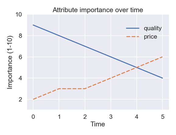
(a) Importance Scores Over Time

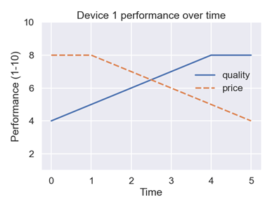
(b) Segment 1 Performance Over Time

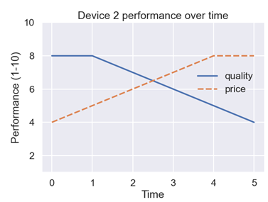
(c) Segment 2 Performance Over Time

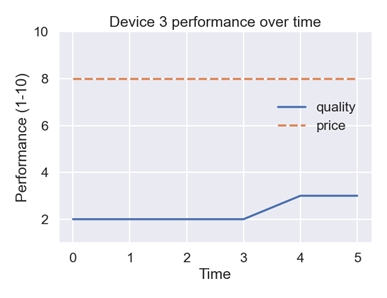
(d) Segment 3 Performance Over Time

Figure 1: Segment Performance Analysis Over Time

We see that over time $t=0\text{ to }6$, $D_{3}$ becomes more competitive in the market while $D_{2}$ becomes less competitive. Ultimately, at $t=6$, $D_{2}$ is the most competitive customer segment in the market. Next, demand is allocated across the three market segments at each time stamp using one of three methodologies—ratio, softmax or redistribution. We also incorporate a winner-take-all factor of 0.3.

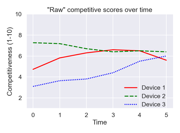
Figure 2: Segment Competitiveness Over Time

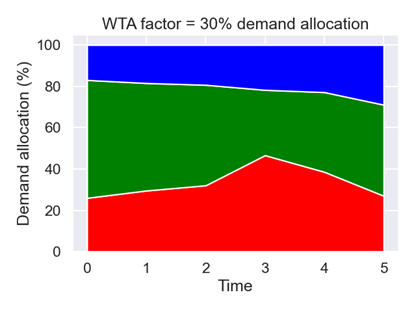
(a) Moderate winner-take-all ($wta=0.3$)

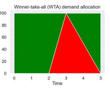
(b) Complete winner-take-all ($wta=1$)

Figure 3: Redistribution-based Demand Allocation Under Different Market Scenarios

We see that in the scenario with $wta=1$, the most competitive device in the market at any $t$ receives 100% of the market demand. In the scenario with $wta=0.3$, we interpolate between a scenario of $wta=1$ and $wta=0$, leaning more closely to the latter. Demand is therefore distributed more proportionally across the three market segments.

9 Future Work

Real-world use cases are likely to have historical market shares and performance estimates, but not customer importance scores or WTA factors. These parameters can be discovered and tuned with constrained optimization. Iteratively collecting and comparing market share data with model predictions can offer important insights. Deviations from model outputs are important learning opportunities and can provide a remedy for speculative forecasting.

10 Conclusion

This paper presents a novel framework for modeling market dynamics that explicitly incorporates product competitiveness and consumer behavior. The key contributions include: (1) a mechanistic modeling framework that moves beyond traditional AR approaches by explicitly modeling underlying market processes, (2) a comprehensive competitiveness scoring system that quantifies product attributes and consumer preferences, and (3) flexible demand allocation mechanisms accommodating different market behaviors from winner-take-all to distributed competitive outcomes.

Our framework addresses fundamental limitations of traditional econometric models by providing causal understanding, enabling scenario analysis, naturally accommodating nonlinear dynamics, and offering interpretable parameters representing real-world processes. The sample implementation demonstrates how competitiveness affects market share evolution, while behavioral factors such as customer psychology provide more nuanced understanding than purely statistical approaches.

By bridging concepts from mathematical biology, dynamical systems theory, and economics, this framework represents a significant step toward more mechanistic, interpretable, and actionable market models that can support strategic decision-making in complex competitive environments.

11 Acknowledgment

We would like to thank our colleagues and management at Intel for providing business use cases and problem statements that motivated our modeling approaches. We are also grateful to the Institute for Operations Research and Management Science (INFORMS) for the opportunity to share our work with the larger OR community.

Appendix A Relationship to Lotka-Volterra Dynamics

The standard LV equations describe the dynamics of two interacting populations:

(31) $$\frac{dx}{dt} =\alpha x-\beta xy$$

(32) $$\frac{dy}{dt} =\delta xy-\gamma y$$

Where $x$ represents prey population, $y$ represents predator population, and the parameters $\alpha,\beta,\gamma,\delta>0$ represent birth rates, predation rates, and death rates.

In our product market model, equation (4) can be rewritten to highlight the analogous structure:

(33) $$\frac{d(D_{i}(t))}{dt}=\underbrace{\frac{d(BND_{i}(t))}{dt}}_{\text{Birth term}}+\underbrace{\frac{d(RD_{i}(t))}{dt}}_{\text{Migration term}}-\underbrace{\frac{d(OD_{i}(t))}{dt}}_{\text{Death term}}$$

The correspondence becomes clearer when we consider the competitive dynamics between market segments:

A.1 Birth and Death Processes

• Birth term $\frac{d(BND_{i}(t))}{dt}$: Analogous to the prey birth rate $\alpha x$ in LV equations, representing the intrinsic growth of segment $i$ through new product introductions.

• Death term $\frac{d(OD_{i}(t))}{dt}$: Analogous to the predator death rate $\gamma y$, representing products becoming obsolete due to technological advancement or market forces.

A.2 Competitive Interactions

The refresh term $\frac{d(RD_{i}(t))}{dt}$ captures the most interesting parallel to LV dynamics. In technology markets, this term can represent:

• Competitive displacement: When superior technology in segment $j$ causes users to abandon segment $i$, similar to predation in LV models

• Market cannibalization: When a company’s new customer segment reduces demand for its existing segments

• Technology migration: Users moving between segments due to changing preferences or capabilities

Appendix B Applications of Dynamical Systems in Economics and Finance

Dynamical systems theory has been successfully applied across various economic and financial domains, providing the foundation for our market modeling approach.

B.1 Macroeconomic Dynamics

Business cycle modeling represents one of the earliest applications of biological dynamics to economics. Employment rates and wage shares interact cyclically in predator-prey fashion, with high employment leading to wage increases that eventually reduce profitability and employment Goodwin (1967). More recent work has developed sophisticated stock-flow consistent models using differential equations that capture dynamic interactions between economic sectors while maintaining accounting identities Grasselli and Maheshwari (2017).

B.2 Behavioral Finance

The most fertile ground for dynamical systems applications has been behavioral finance, where psychological factors and social interactions drive market dynamics. Models of herd behavior explain how rational individual decisions can lead to collective market bubbles and crashes through purely endogenous mechanisms Lux (1995).

These applications demonstrate key advantages of dynamical systems approaches: they model rates of change rather than levels, incorporate nonlinear relationships and feedback effects, provide mechanistic explanations for observed phenomena, and enable scenario analysis. Our market segmentation model builds on these foundations to address the specific challenges of modeling competitive dynamics in technology markets.

References

- Anderson and May [1991] Roy M. Anderson and Robert M. May. Infectious diseases of humans: dynamics and control. Oxford University Press, Oxford, 1991. URL https://global.oup.com/academic/product/infectious-diseases-of-humans-9780198545996.
- Arthur et al. [1997] W. Brian Arthur, Steven N. Durlauf, and David A. Lane, editors. The economy as an evolving complex system II. Addison-Wesley, Reading, MA, 1997. URL https://www.santafe.edu/research/results/books/the-economy-as-an-evolving-complex-system-ii.
- Bergmeir and Benítez [2012] Christoph Bergmeir and José M. Benítez. On the use of cross-validation for time series predictor evaluation. Information Sciences, 191:192–213, 2012. URL https://doi.org/10.1016/j.ins.2011.12.028.
- Bergstrom [1990] A. R. Bergstrom. Continuous time econometric modelling. Oxford University Press, Oxford, 1990. URL https://global.oup.com/academic/product/continuous-time-econometric-modelling-9780198283409.
- Blanchard and Kahn [1980] Olivier J. Blanchard and Charles M. Kahn. The solution of linear difference models under rational expectations. Econometrica, 48(5):1305–1311, 1980. URL https://doi.org/10.2307/1912186.
- Box and Jenkins [1976] George E. P. Box and Gwilym M. Jenkins. Time series analysis: forecasting and control. Holden-Day, San Francisco, 1976.
- Brunel [2008] Nicolas J.-B. Brunel. Parameter estimation of ODE’s via nonparametric estimators. Electronic Journal of Statistics, 2:1242–1267, 2008. URL https://doi.org/10.1214/07-EJS132.
- Burnham and Anderson [2002] Kenneth P. Burnham and David R. Anderson. Model selection and multimodel inference: a practical information-theoretic approach. Springer, New York, 2002. URL https://doi.org/10.1007/b97636.
- Chintagunta and Vilcassim [1992] Pradeep K. Chintagunta and Naufel J. Vilcassim. An empirical investigation of advertising strategies in a dynamic duopoly. Management Science, 38(9):1230–1244, 1992. URL https://doi.org/10.1287/mnsc.38.9.1230.
- Day and Huang [1990] Richard H. Day and Weihong Huang. Bulls, bears and market sheep. Journal of Economic Behavior & Organization, 14(3):299–329, 1990. URL https://doi.org/10.1016/0167-2681(90)90061-H.
- Epstein and Pojman [1998] Irving R. Epstein and John A. Pojman. An introduction to nonlinear chemical dynamics: oscillations, waves, patterns, and chaos. Oxford University Press, Oxford, 1998. URL https://global.oup.com/academic/product/an-introduction-to-nonlinear-chemical-dynamics-9780195096705.
- Farmer and Foley [2009] J. Doyne Farmer and Duncan Foley. The economy needs agent-based modelling. Nature, 460(7256):685–686, 2009. URL https://doi.org/10.1038/460685a.
- Goodwin [1967] Richard M. Goodwin. A growth cycle. In C. H. Feinstein, editor, Socialism, Capitalism and Economic Growth, pages 54–58. Cambridge University Press, Cambridge, 1967.
- Granger [1969] Clive W. J. Granger. Investigating causal relations by econometric models and cross-spectral methods. Econometrica, 37(3):424–438, 1969. URL https://doi.org/10.2307/1912791.
- Grasselli and Maheshwari [2017] Matheus Grasselli and Aditya Maheshwari. A comment on ‘Testing Goodwin: growth cycles in ten OECD countries’. Cambridge Journal of Economics, 41(6):1761–1766, 2017. URL https://doi.org/10.1093/cje/bex006.
- Hamilton [1989] James D. Hamilton. A new approach to the economic analysis of nonstationary time series and the business cycle. Econometrica, 57(2):357–384, 1989. URL https://doi.org/10.2307/1912559.
- Hamilton [1994] James D. Hamilton. Time series analysis. Princeton University Press, Princeton, NJ, 1994. URL https://press.princeton.edu/books/hardcover/9780691042893/time-series-analysis.
- Hanssens et al. [2001] Dominique M. Hanssens, Leonard J. Parsons, and Randall L. Schultz. Market response models: econometric and time series analysis. Springer, New York, 2001. URL https://doi.org/10.1007/978-1-4615-1701-4.
- Hendry [1995] David F. Hendry. Dynamic econometrics. Oxford University Press, Oxford, 1995. URL https://global.oup.com/academic/product/dynamic-econometrics-9780198283164.
- Lucas [1976] Robert E. Jr. Lucas. Econometric policy evaluation: A critique. Carnegie-Rochester Conference Series on Public Policy, 1:19–46, 1976. URL https://doi.org/10.1016/S0167-2231(76)80003-6.
- Lütkepohl [2005] Helmut Lütkepohl. New introduction to multiple time series analysis. Springer, Berlin, 2005. URL https://doi.org/10.1007/978-3-540-27752-1.
- Lux [1995] Thomas Lux. Herd behaviour, bubbles and crashes. Economic Journal, 105(431):881–896, 1995. URL https://doi.org/10.2307/2235156.
- Medio and Lines [2001] Alfredo Medio and Marji Lines. Nonlinear dynamics: a primer. Cambridge University Press, Cambridge, 2001. URL https://doi.org/10.1017/CBO9780511754050.
- Murray [2002] James D. Murray. Mathematical biology: I. An introduction. Springer, New York, 3rd edition, 2002. URL https://doi.org/10.1007/b98868.
- Pearl [2009] Judea Pearl. Causality. Cambridge University Press, Cambridge, 2nd edition, 2009. URL https://doi.org/10.1017/CBO9780511803161.
- Pesaran and Timmermann [2007] M. Hashem Pesaran and Allan Timmermann. Selection of estimation window in the presence of breaks. Journal of Econometrics, 137(1):134–161, 2007. URL https://doi.org/10.1016/j.jeconom.2006.03.010.
- Phillips [1991] Peter C. B. Phillips. Optimal inference in cointegrated systems. Econometrica, 59(2):283–306, 1991. URL https://doi.org/10.2307/2938258.
- Ramsay et al. [2007] James O. Ramsay, Giles Hooker, David Campbell, and Jiguo Cao. Parameter estimation for differential equations: a generalized smoothing approach. Journal of the Royal Statistical Society: Series B (Statistical Methodology), 69(5):741–796, 2007. URL https://doi.org/10.1111/j.1467-9868.2007.00610.x.
- Saari [1985] Donald G. Saari. Iterative price mechanisms. Econometrica, 53(5):1117–1131, 1985. URL https://doi.org/10.2307/1911017.
- Scarf [1960] Herbert Scarf. Some examples of global instability of the competitive equilibrium. International Economic Review, 1(3):157–172, 1960. URL https://doi.org/10.2307/2525561.
- Sims [1980] Christopher A. Sims. Macroeconomics and reality. Econometrica, 48(1):1–48, 1980. URL https://doi.org/10.2307/1912017.
- Stock and Watson [1996] James H. Stock and Mark W. Watson. Evidence on structural instability in macroeconomic time series relations. Journal of Business & Economic Statistics, 14(1):11–30, 1996. URL https://doi.org/10.1080/07350015.1996.10524626.
- Strogatz [2014] Steven H. Strogatz. Nonlinear dynamics and chaos: with applications to physics, biology, chemistry, and engineering. Westview Press, Boulder, CO, 2nd edition, 2014. URL https://www.westviewpress.com/books/nonlinear-dynamics-and-chaos.
- Teräsvirta et al. [2005] Timo Teräsvirta, Dick Van Dijk, and Marcelo C. Medeiros. Linear models, smooth transition autoregressions, and neural networks for forecasting macroeconomic time series: A re-examination. International Journal of Forecasting, 21(4):755–774, 2005. URL https://doi.org/10.1016/j.ijforecast.2005.04.010.
- Tong [1990] Howell Tong. Non-linear time series: a dynamical system approach. Oxford University Press, Oxford, 1990. URL https://global.oup.com/academic/product/non-linear-time-series-9780198522249.
- Tritton [1988] D. J. Tritton. Physical fluid dynamics. Oxford University Press, Oxford, 2nd edition, 1988. URL https://global.oup.com/academic/product/physical-fluid-dynamics-9780198544937.
- Wiggins [2003] Stephen Wiggins. Introduction to applied nonlinear dynamical systems and chaos. Springer, New York, 2nd edition, 2003. URL https://doi.org/10.1007/b97481.
- Zeeman [1974] E. Christopher Zeeman. On the unstable behaviour of stock exchanges. Journal of Mathematical Economics, 1(1):39–49, 1974. URL https://doi.org/10.1016/0304-4068(74)90034-2.