Testing the equality of estimable parameters across many populations
Abstract
The comparison of a parameter in populations is a classical problem in statistics. Testing for the equality of means or variances are typical examples. Most procedures designed to deal with this problem assume that is fixed and that samples with increasing sample sizes are available from each population. This paper introduces and studies a test for the comparison of an estimable parameter across populations, when is large and the sample sizes from each population are small when compared with . The proposed test statistic is asymptotically distribution-free under the null hypothesis of parameter homogeneity, enabling asymptotically exact inference without parametric assumptions. Additionally, the behaviour of the proposal is studied under alternatives. Simulations are conducted to evaluate its finite-sample performance, and a linear bootstrap method is implemented to improve its behaviour for small . Finally, an application to a real dataset is presented.
Keywords: Testing Many populations -statistics Consistency
1 Introduction
Testing the equality of a parameter in a given number of populations from independent samples coming from them, is a central topic in statistics, with early methods including one-way ANOVA for comparing means (Fisher,, 1925) and Bartlett’s test for comparing variances (Bartlett,, 1937). Given the sensitivity of these procedures to parametric assumptions, nonparametric alternatives such as the Kruskal–Wallis’ test (Kruskal and Wallis,, 1952) and Levene’s test (Levene,, 1960) were later developed.
These classical methods implicitly assume that the number of populations is fixed and small relative to the within-group sample sizes , which are usually assumed to be large. In many contemporary applications, such as genomics (see e.g. Zhan and Hart, (2014)) or social sciences (see e.g. Alba-Fernández et al., (2024)), researchers frequently face problems where is large and larger than the sample sizes from each population. In an era of massive data collection, comparing fundamental parameters, such as measures of location, dispersion, or association, across many groups remains an interesting problem.
The behavior of some classical tests in the large-, small- regime has been studied in the literature for some specific testing problems. Below, we cite some papers dealing with the comparison of means. Boos and Brownie, (1995) analyzed the asymptotic properties of ANOVA and rank-based tests as , assuming homoscedasticity. Building on this work, Akritas and Arnold, (2000) derived the asymptotic distribution of the ANOVA -statistic in both one-way and two-way layout models. Subsequently, Bathke, (2002) extended the analysis to the balanced multi-factor case, demonstrating that the asymptotic properties observed in simpler layouts can be generalized to more complex factorial designs. Later, Akritas and Papadatos, (2004) introduced nonparametric procedures for one-way layouts that accommodate heteroscedasticity, thereby broadening the applicability of multi-sample inference in large- settings. Collectively, these studies show that classical -statistics and their rank-based analogues, under the assumption of homoscedasticity, converge in distribution to a normal law as , deviating from the classical distribution. This shift (which not only happens in the tests for the means) highlights the necessity of either adapting existing tests or developing novel statistical methods specially designed for the large-, small- context.
Motivated by these challenges, some recent research is focused on multi-sample inference with large and small sample sizes for testing other hypothesis rather than comparing means. Specifically, goodness-of-fit tests have been designed for this regime, with recent contributions addressing Poissonity, normality, and proportion tests in Jiménez-Gamero and de Uña Álvarez, (2024), Jiménez-Gamero, (2024), Alba-Fernández et al., (2024), respectively; approaches for the -sample problem have also been developed by Zhan and Hart, (2014), Kim, (2021), and Jiménez-Gamero et al., (2022); a test for homocedasticity has been proposed in Jiménez-Gamero et al., (2025).
In particular, in their practical application, Zhan and Hart, (2014) rejected the null hypothesis of equal densities, suggesting the presence of heterogeneity across the populations. This naturally raises the question of whether the observed differences are driven by specific parameters such as the mean, variance, or other distributional characteristics. Investigating these aspects could provide a deeper understanding of the nature of the heterogeneity detected by the test.
While much of the existing work has focused on comparing means, variances, or entire distributions, it is natural to consider broader comparisons involving parameters such as measures of location, scale, dispersion, association, or other functionals expressible as expectations of kernels. In this way, the comparison of means and variances can be extended to other population parameters, such as the Gini mean difference and Spearman’s rho. In this direction, the framework developed in this paper provides a unified approach to compare such parameters across many populations without relying on specific structural properties of the kernel.
In this work, assuming independent samples from each population, the problem of testing the null hypothesis is considered, where each is defined as the expectation of a kernel of fixed degree . A test statistic is proposed, which is an unbiased estimator of the variance of the parameters . Notice that is equivalent to . Under some mild assumptions, is consistent and asymptotically normal, where by asymptotic we mean as . The asymptotic distribution of is derived by decomposing it into a linear component and a remainder. The variance of the reminder is shown to be is asymptotically negligible relative to that of the linear part. The practical use of as a test statistic, requires the estimation of its asymptotic variance, which is the variance of its linear component. A ratio-consistent estimator of the variance under the null hypothesis is devised. This way, it is obtained a test statistic which is asymptotically free distributed under the null. The power of the proposed test is analyzed for a broad class of alternatives, establishing its consistency under explicit conditions on the rate at which alternatives converge to the null and the growth of the sample sizes.
To improve the performance of the proposed procedure for moderate and small values of we additionally implement a bootstrap procedure. The behavior of the asymptotic approximation and the bootstrap approximation are assessed through an extensive simulation study focusing on the Gini mean difference and Spearman’s rho.
One of the assumed assumptions to derive the previous results is that the sample sizes must be comparable (in a sense that will be specified later). When applying our methodology to real datasets, we found that the sample sizes were far from balanced, with some being very large. Another point is that the computation of the variance of the test statistic increases substantially with the sample sizes. To deal with these two issues, we adopt a strategy which parallels to that in Cuesta-Albertos and Febrero-Bande, (2010). Specifically, balanced random samples are taken from the data and the associated -value is obtained. This is repeated several times and the -values are adjusted.
The remainder of the paper is organized as follows. Section 2 introduces the proposed test statistic for comparing general parameters across multiple populations. Section 3 develops the asymptotic distribution of the test statistic under the null hypothesis. Section 4 presents a ratio-consistent estimator for the asymptotic variance. Section 5 studies the asymptotic power of the proposed test under various types of alternatives. Section 6 discusses computational challenges and proposed solutions.
2 Test statistic
Let be independent random elements defined on a common probability space , taking values in a measurable space , where is an arbitrary space and is -algebra on .
Furthermore, let be a fixed integer. We consider that
| (1) | ||||
Let be defined as
where is a symmetric kernel of degree . For this kernel, we denote its variance terms as
| (2) |
where .
Our objective is to test when is large. Under the null, this is equivalent to testing whether , where
with .
Given the definition of the parameter , it is natural to estimate it using the -statistic
where , which is an unbiased estimator of for . Similarly, to obtain an unbiased estimator of , we first construct a unbiased estimators of for by applying -statistics theory. The kernel associated with is
| (3) |
and the corresponding unbiased estimator of is given by
Then, we define the statistic
| (4) |
which is, by construction, an unbiased estimator of . Moreover, under certain conditions, is a consistent estimator of , meaning that converges in probability to . Specifically, we assume that
| (5) |
which is a key assumption in most of our results to derive meaningful conclusions. Throughout this paper, all limits are understood to be taken as , unless otherwise specified.
The null hypothesis is identified by , whereas the alternative hypothesis is characterized by . Since is unbiased and consistent for , it would be reasonable to reject when is large. However, to determine when is large, we need to know its distribution under . Since we have made no assumptions about the underlying distribution of , obtaining the exact distribution of is not feasible. For this reason, we approximate it through its asymptotic distribution, which is derived in the next section.
3 Asymptotic distribution
To derive the asymptotic distribution of , we decompose the statistic as stated in the following lemma:
Lemma 2.
can be expressed as
| (6) |
where
and
Note that the variable depend only on the sample . As the samples are independent, the variables are also independent. Consequently,
| (7) |
Lemma 3.
Assume that . The variance of is given by
where
Now, we outline the scenarios in which we will obtain the asymptotic distribution of . We consider two cases. The first case is the obvious one, where holds. If is not true, we assume one of the following assumptions describing the behavior of the sequence .
Assumption 1.
does not hold, one of these conditions is satisfied:
-
(i)
, for some and some .
-
(ii)
and for some and some , where is an increasing sequence such that , , for some , and , , for some positive constant .
Condition (i) corresponds to a scenario where remains bounded away from zero for all sufficiently large . In contrast, condition (ii) allows to approach zero at a controlled rate , since
| (8) |
These two conditions are assumed to ensure that the sequence behaves regularly, allowing us to derive meaningful outcomes.
To establish the asymptotic distribution of the test statistic, we will show that the variance of the remainder term is negligible compared to the variance of the linear term. To achieve this, we make two additional assumptions.
First, we assume that the sample sizes are comparable, in the sense that
| (9) |
The comparability condition on sample sizes, as defined in (9), is imposed to mitigate the impact of severe sample size imbalances, which affects the asymptotic distribution of the statistic. Such assumption is commonly made in the statistical literature. For instance, Scholz and Stephens, (1987) and Rizzo and Székely, (2010) impose similar conditions to establish the consistency of the test developed in their respective works. In what follows, we omit the explicit dependence on of and for simplicity in notation.
Next, we assume that is non-degenerate, meaning that , where is defined in (2). Morover, to derive the next result we assume a uniform lower bound on , i.e.,
| (10) |
Lemma 4.
Once we have the previous result, deriving the asymptotic distribution of reduces to determining the asymptotic distribution of , which is stated in the following result.
Lemma 5.
Theorem 1.
Under the assumptions of Lemma 5, we have that .
Theorem 1 holds either if is true or Assumption 1 is satisfied. Specifically, when holds, we have , and from (7), it follows that . As discussed at the end of Section 2, it is reasonable to reject the null hypothesis whenever is large, as larger values of indicate a stronger deviation from . Theorem 1 provides a rigorous foundation for constructing statistical tests. Specifically, for a chosen significance level , we can reject if , where is the critical value corresponding to the -quantile of the standard normal distribution. This decision rule ensures that the probability of incorrectly rejecting (the type I error) does not exceed for large .
However, in practice, Theorem 1 cannot be directly applied because the variance is typically unknown, as no assumptions are made about the distribution of the random variables. To address this limitation, we require a ratio-consistent estimator of under . Specifically, this means that when holds. By Slutsky’s theorem, substituting with in the normalization does not alter the limiting distribution. Consequently, constructing such an estimator is a crucial step for the practical implementation of the test. The details of this construction are presented in the following section.
Remark 1.
Note that all previous results are valid whenever the sample sizes satisfy (9), which allows the sample size to remain bounded or increase with .
4 Variance estimation
The variance we are trying to estimate, as defined in (7), is given by
Firstly, we eliminate the aditive constants in , as they have no effect in the variance computation. For that, we introduce the auxiliar quantities
| (11) |
and by construction, we have that for . Observe that , and therefore, . Let
Its expetation is given by
where and . We have that,
with . Therefore we can write
where
| (12) |
It is easy to observe that, under , , and hence . However, although could serve as a ratio-consistent estimator of , it cannot be directly computed because are unknown, as is unknown. To address this issue, we introduce a slight modification. Define
and
| (13) |
Finally, we show that is a ratio-consistent estimator of , as formally stated in the following result.
Proposition 1.
In contrast to the results previously stated, the ratio-consistency of in Proposition 1 additionally requires that . This assumption is not particularly restrictive in practice, as it is generally unrealistic to obtain increasing amounts of data from all populations as the number of populations grows. Furthermore, the proposition assumes the existence of a -th moment for some . This condition is justified in each of the cases considered, since Lemma 9 (parts 1, 3, 4, and 5) in Section 10 shows that the corresponding variables, , , or , have finite second moments. In light of this, it is reasonable to impose a slightly stronger moment condition in each setting.
Observe that under , since , the variance estimator satisfies the ratio-consistency property, i.e., . Recalling Theorem 1 and applying Slutsky’s theorem, it follows that
| (14) |
Consequently, the test that rejects if has level asymptotically.
5 Asymptotic power
In this section, we study the asymptotic power of the proposed test under the alternatives outlined in Assumption 1. The following theorem summarizes the cases in which the test is consistent, i.e., , where .
Theorem 2.
Assume that the conditions in Proposition 1 are satisfied, and that one of the following scenarios holds:
-
a)
Assumption 1.i is satisfied.
-
b)
Assumption 1.ii is satisfied and .
-
c)
Assumption 1.ii is satisfied, , and .
-
d)
Assumption 1.ii is satisfied, , , and remains bounded.
-
e)
Assumption 1.ii is satisfied, , , , and .
Then, .
The following results examine the power of the test under alternative scenarios, where the asymptotic power is less than .
Proposition 2.
The results presented above are based on the possible behaviors of the sequences and . These include cases where is bounded or tends to infinity, as well as different rates at which and approach infinity. They provide intuitive insights into the asymptotic power of the test, which can be summarized as follows:
-
•
Alternatives satisfying Assumption 1.i, where is bounded away from zero, can be detected by the test both when is bounded and when (case (a)).
-
•
For alternatives satisfying Assumption 1.ii, the behavior depends on the rate at which converges to zero. The following subcases can be distinguished:
-
–
If (case (b)), converges to 0 at a slow rate, allowing the test to detect the violation of both when is bounded and when .
-
–
If (i.e., ; case (c) and Proposition 2.1 , converges faster than in the previous case, and a bounded is no longer sufficient. Consistency is achieved when . On the other hand, if remains bounded, the power converges to a value strictly between and 1. This value depends on the limiting behavior of the signal-to-noise ratio , and is equal to when this quantity converges to .
-
–
For the final cases, where (cases (d) and (e) in Theorem 2, and parts 2–3 of Proposition 2, converges to zero so fast that the consistency of the test is achieved if at a rate faster than a certain threshold. In particular, consistency is achieved when . Otherwise, the test is consistent when grows faster than . Finally, when , the power tends to a value in , which again depends on the limiting signal-to-noise ratio. If instead , then the power tends to .
-
–
All above cases are graphically displayed in Figure 1.
This discussion shows that the more difficult it is to detect the violation of , the larger the number of observations in each group must be to ensure consistency. While easier alternatives can be detected with a bounded , more challenging ones require not only , but also at a fast enough rate.
6 Computational considerations
The practical application of the proposed methodology may face two main challenges. First, the behavior of the test statistic may deviate from its asymptotic distribution, particularly when the number of groups is small or moderate. Second, when group sizes are large or highly unbalanced, both the computational burden and the validity of the theoretical approximations may be adversely affected. To address these challenges, we propose two complementary strategies:
-
•
A linear bootstrap procedure to improve the practical performance of the test for small to moderate .
-
•
A random sampling approach that reduces the computational burden and mitigates the impact of group size imbalance.
6.1 Linear bootstrap
In the simulation study, the convergence to the normal law of the null distribution of the test statistic was found to be relatively slow for small to moderate . To improve the performance of the test, we employed a linear bootstrap procedure based on resampling the linear component of the statistic, as proposed in Jiménez-Gamero et al., (2025). The procedure is implemented as follows:
-
1.
Compute the centered linear components .
-
2.
Generate a bootstrap sample from the empirical distribution of the centered values.
-
3.
Evaluate the linear approximation of on the bootstrap sample, obtaining , where and .
-
4.
Approximate the null distribution of by the conditional distribution of given the observed data .
In practice, this approximation is computed via Monte Carlo simulation: steps 2 and 3 are repeated times, yielding bootstrap replicates . The empirical distribution of these replicates provides an estimate of the linear bootstrap distribution of .
This resampling strategy is particularly efficient for large , as it completely avoids the computation of at bootstrap level, which are the most computationally demanding components of the statistic.
6.2 Random sampling
Real datasets often exhibit considerable imbalance in sample sizes, with some groups having disproportionately large sizes. This fact poses three issues: a) to derive the results, comparability of sample sizes is assumed (see (9)); b) the sample sizes must be small relative to (recall that Proposition 1 assumes that ); c) the estimation of the variance requires computing , each based on a -statistic of degree with computational cost for , and hence, the overall computational burden may become substantially large.
To address these limitations, we propose a random sampling scheme whereby, for each application of the test, we draw a sample of size from each group. This reduces the computational burden and provides a better approximation to the condition in Proposition 1. It is worth noting that different random samples may lead to contradictory conclusions. To mitigate this problem, we adopt the strategy proposed by Cuesta-Albertos and Febrero-Bande, (2010) in the context of random projection tests for functional data. Their approach consists in generating independent random projections, computing the -value for each of them, and applying a multiple testing correction (such as the method proposed in Benjamini and Yekutieli, (2001)). Specifically, their methodology computes -values, one for each random projection; then sorts them as ; and finally obtains the -value as . The global null hypothesis is then rejected at level whenever . Proposition 2.3 in Cuesta-Albertos and Febrero-Bande, (2010) ensures that the level is at most .
In our setting, we apply the same idea by drawing independent random samples from each group; calculating the -value for each set of random samples and calculating as before. The authors recommend the use up to . Furthermore, as shown in Theorem 2, some alternatives require to increase with in order to ensure the consistency of the test. Consequently, rather than fixing a small sample size in advance, we adopt an adaptive strategy in which is progressively increased until the test decision stabilizes.
7 Simulation studies
In this section, we evaluate the finite-sample performance of the proposed test through Monte Carlo simulations selecting a particular choice of the kernel . We have selected two different statistics to evaluate the performance of the test: the Gini mean difference (GMD) and the Spearman’s rho . We assess the performance of two tests:
-
•
The test based on the asymptotic normal approximation derived in this work (N).
-
•
The linear bootstrap test discussed in Section 6 (LB).
To reduce the computational burden involved in bootstrap, we employ the warp-speed method proposed in Giacomini et al., (2013). In this approach, instead of computing critical values for each Monte Carlo sample, we generate a single resample per iteration. Let denote the total number of Monte Carlo replications. In each iteration , the test statistic is first computed on the original sample, resulting in , and then on a resample generated in the same iteration, yielding . The empirical distribution of the resampled statistics, , is then used to compute -values for the corresponding original values , .
For each configuration, we generate independent samples from populations, with identical sample sizes . The -value of the observed value of the test statistic is computed using both the normal approximation and the bootstrap approach. The simulation is repeated times to estimate the empirical rejection rates under the null and alternative hypotheses. We study the impact of both the number of populations and the individual sample size on the performance of the test.
7.1 Gini mean difference
The Gini mean difference (GMD) of a random variable is defined as , where and are independent copies of . This corresponds to a -statistic of degree 2 with kernel .
Type I error: Experimental design and results
To empirically asses the probability of type I error, we considered four data-generating settings. In the first three, all populations are identically distributed, following:
-
1.
a standard normal distribution ,
-
2.
a chi-squared distribution with 3 degrees of freedom, ,
-
3.
a Student’s -distribution with 5 degrees of freedom ,
-
4.
A heterogeneous mixture: one third of the populations are sampled from each of the aforementioned distributions, and the data are rescaled so that all populations have a Gini mean difference equal to 1.
For each case, we considered populations and equal group sizes for . The results are reported in Table 1.
| 50 N 4.4 9.5 3.2 7.7 3.1 7.4 LB 4.6 9.4 4.7 9.6 4.7 9.9 100 N 4.5 9.5 3.4 8.4 3.4 8.4 LB 5.0 10.1 4.3 9.2 5.0 10.2 500 N 4.5 9.4 4.3 8.8 4.0 9.1 LB 4.5 9.4 5.3 10.0 5.0 10.3 1000 N 4.6 9.9 4.3 9.3 4.2 9.0 LB 4.8 9.9 5.0 10.1 5.0 10.1 1500 N 4.7 9.8 4.3 8.9 4.3 9.1 LB 4.9 10.1 4.6 9.8 4.8 9.6 50 N 4.9 9.9 4.0 9.0 3.6 8.8 LB 3.6 8.7 3.9 9.3 4.1 10.0 100 N 4.8 10.1 4.0 9.1 3.8 8.2 LB 4.3 9.7 4.1 9.4 4.3 8.5 500 N 4.9 9.9 4.6 9.4 4.2 8.8 LB 4.7 9.6 4.8 9.8 4.7 9.9 1000 N 4.4 9.6 4.6 9.6 4.6 9.6 LB 5.0 9.8 4.8 9.6 4.7 10.3 1500 N 4.7 9.9 4.8 9.7 4.7 9.9 LB 4.7 10.0 5.1 9.8 5.0 10.1 |
| Test 50 N 3.9 8.8 3.2 8.1 3.4 8.1 LB 3.3 8.3 3.6 8.2 4.5 9.3 100 N 4.1 8.8 3.2 8.2 3.4 8.2 LB 4.0 8.8 3.8 8.9 4.5 10.2 500 N 4.1 9.0 3.8 9.3 3.9 8.5 LB 5.0 9.6 4.5 9.9 4.8 9.9 1000 N 4.4 9.4 4.2 9.2 4.2 9.2 LB 4.7 9.8 5.0 9.9 5.1 9.6 1500 N 4.6 9.9 4.2 9.2 4.3 9.4 LB 4.9 10.3 5.2 9.8 5.0 10.3 Mixture 50 N 4.5 9.8 3.7 8.7 3.2 8.1 LB 3.5 8.8 3.7 9.0 3.9 8.6 100 N 4.3 9.3 4.0 8.9 3.5 8.3 LB 4.1 9.4 4.4 9.8 4.2 9.6 500 N 4.4 9.4 4.3 9.4 4.3 9.2 LB 4.4 9.2 5.2 10.1 5.1 10.4 1000 N 4.3 9.2 4.4 9.4 4.2 9.1 LB 4.8 9.4 5.2 9.9 4.8 9.6 1500 N 4.7 9.7 4.1 9.4 4.3 9.3 LB 5.2 10.3 4.7 10.2 4.6 9.7 |
Looking at Table 1, we observe that that both the asymptotic test (N) and the linear bootstrap test (LB) tend to be conservative for small . For small values of , increasing the sample size can lead to a decrease in the empirical type I error rate, specially for the asymptotic test. As the number of populations increases, both procedures converge to the nominal levels. In general, the bootstrap test display a better performance.
Empirical power: Experimental design and results
We generated scaled normal data with and created alternatives by assigning a proportion of contaminated data with of the populations with GMD equal to . We considered configurations with and . In this case, we have that . Therefore, by varying and , we assess the power of the test under alternatives located at different distances from the null. The results obtained are reported in Table 2.
| Test | ||||||||
| 0.1 | 50 | N | 5.5 11.0 | 5.9 12.7 | 7.8 16.5 | 7.5 14.6 | 13.4 25.6 | 23.5 40.5 |
| LB | 5.7 10.9 | 8.7 15.7 | 11.2 20.7 | 7.7 14.9 | 18.4 31.0 | 30.9 47.0 | ||
| 100 | N | 5.8 11.9 | 8.1 16.6 | 11.8 22.8 | 9.3 17.4 | 24.0 38.7 | 44.5 62.3 | |
| LB | 6.4 12.8 | 10.5 18.9 | 16.1 28.0 | 10.4 18.7 | 28.1 42.6 | 53.6 68.9 | ||
| 200 | N | 6.8 13.3 | 11.1 21.2 | 19.0 32.2 | 12.7 22.5 | 41.1 57.6 | 74.0 85.7 | |
| LB | 7.6 14.7 | 13.6 23.8 | 22.9 35.9 | 14.2 24.1 | 45.3 60.8 | 78.5 87.8 | ||
| 0.2 | 50 | N | 6.4 12.6 | 9.2 18.2 | 14.9 27.6 | 11.5 20.9 | 33.0 50.2 | 61.6 77.9 |
| LB | 6.4 12.8 | 12.6 22.6 | 20.8 33.0 | 11.6 21.3 | 40.4 56.0 | 69.0 82.6 | ||
| 100 | N | 7.3 14.2 | 14.6 25.9 | 25.7 41.1 | 16.0 27.1 | 57.9 73.1 | 89.8 95.6 | |
| LB | 8.2 15.1 | 17.2 28.4 | 32.5 47.1 | 17.8 28.6 | 62.2 76.6 | 93.1 96.5 | ||
| 200 | N | 9.2 17.1 | 22.7 36.9 | 44.5 60.9 | 25.3 38.8 | 85.5 92.3 | 99.6 99.9 | |
| LB | 10.5 18.4 | 26.4 40.4 | 51.0 64.7 | 27.6 40.7 | 87.5 93.4 | 99.8 99.9 | ||
| 0.3 | 50 | N | 7.1 14.3 | 12.3 23.5 | 22.4 37.7 | 15.7 26.4 | 53.1 69.7 | 86.1 93.7 |
| LB | 7.6 14.7 | 16.6 28.3 | 29.3 44.2 | 16.4 27.5 | 60.3 74.2 | 89.5 95.5 | ||
| 100 | N | 8.7 16.4 | 21.1 34.5 | 40.1 56.0 | 23.1 36.7 | 81.2 90.2 | 98.9 99.7 | |
| LB | 9.5 17.6 | 24.6 37.9 | 47.5 61.0 | 25.5 38.9 | 84.4 91.7 | 99.4 99.8 | ||
| 200 | N | 11.6 20.9 | 35.1 50.8 | 66.1 79.1 | 38.8 54.0 | 97.8 99.3 | 100 100 | |
| LB | 13.1 22.4 | 40.9 54.7 | 71.9 81.7 | 42.6 56.0 | 98.5 99.5 | 100 100 | ||
| 0.4 | 50 | N | 7.5 14.9 | 15.1 27.4 | 28.6 45.3 | 18.6 30.7 | 65.8 79.9 | 94.3 97.9 |
| LB | 8.0 15.3 | 19.8 32.5 | 36.5 51.9 | 20.7 31.7 | 72.7 83.3 | 96.3 98.5 | ||
| 100 | N | 9.5 17.9 | 26.1 40.6 | 49.7 65.7 | 29.5 44.2 | 91.4 96.1 | 99.9 100 | |
| LB | 10.7 19.1 | 30.2 44.9 | 56.9 70.3 | 33.2 47.0 | 93.2 96.8 | 100 100 | ||
| 200 | N | 13.4 23.2 | 43.9 60.2 | 78.1 88.1 | 49.6 64.6 | 99.7 99.9 | 100 100 | |
| LB | 14.8 24.1 | 49.4 64.1 | 82.9 89.9 | 53.3 66.0 | 99.8 100 | 100 100 | ||
As can be seen in Table 2, the empirical power increases with higher values of , , and . The bootstrap approximation slightly outperforms the asymptotic approach.
7.2 Spearman’s rho
The Spearman’s rho between the -th and -th components of a -dimensional random vector is defined as
where , and are independent copies of , and is a symmetric kernel of degree 3 given by
The superscripts and indicate the -th and -th components of the vectors , respectively. This -statistic representation can be found in Maache and Lepage, (2003)
Type I error: Experimental design and results
To empirically assess the probability of type I error of the test when the parameter of interest is Spearman’s rho, we generated data from bivariate normal distributions with varying degrees of correlation between two components. Specifically, we considered Spearman’s rho values , populations, and group sizes .
| Test 50 N 4.3 9.4 3.3 7.8 3.0 7.6 LB 4.6 10.2 5.1 9.7 4.8 9.3 100 N 4.3 9.4 4.0 8.9 3.4 8.0 LB 5.1 9.9 4.9 10 4.8 9.8 500 N 4.8 9.7 4.4 9.5 3.9 8.4 LB 4.9 10.4 4.8 9.8 4.8 9.3 1000 N 4.7 9.8 4.5 9.6 4.3 9.4 LB 4.7 10.1 5.2 10.2 4.9 10.1 1500 N 4.5 9.6 4.7 9.6 4.6 9.5 LB 4.8 9.8 5.3 10.2 5.4 10.2 2000 N 4.5 9.5 4.7 9.8 4.7 9.7 LB 4.7 10.0 5.2 10.4 5.3 10.5 Test 50 N 3.8 8.7 2.9 7.3 2.8 7.2 LB 4.4 9.7 4.2 8.9 4.7 9.5 100 N 3.9 8.3 3.2 7.8 3.0 7.8 LB 4.7 9.8 4.8 9.6 4.5 9.6 500 N 4.2 9.2 3.8 8.5 3.9 9.0 LB 4.6 9.2 4.5 9.8 4.7 10.4 1000 N 4.5 9.6 4.4 8.9 4.2 8.8 LB 4.7 9.5 5.1 9.6 4.9 9.4 1500 N 4.6 9.6 4.3 9.3 4.0 8.7 LB 4.7 10.0 4.7 10.2 4.6 10.0 2000 N 4.6 9.6 4.6 9.2 4.0 8.9 LB 4.9 9.9 5.2 9.9 4.6 9.8 |
| Test 50 N 2.5 6.7 2.4 6.5 2.4 6.5 LB 3.4 8.6 3.8 8.4 3.8 8.7 100 N 2.8 7.2 2.9 7.3 2.6 6.9 LB 4.2 9.0 5.0 9.8 4.0 8.9 500 N 3.6 8.3 3.4 8.2 3.5 8.5 LB 4.5 9.3 4.5 9.5 4.4 9.8 1000 N 4.2 8.7 4.0 0.1 4.0 8.6 LB 4.8 9.6 5.2 10.2 4.7 9.4 1500 N 4.2 9.1 4.3 9.2 4.2 8.6 LB 4.7 9.5 5.2 10.3 5.0 9.9 2000 N 4.4 9.6 4.5 9.2 4.3 8.9 LB 4.5 10.0 5.3 10.2 5.4 10.1 Test 50 N 1.1 4.3 1.7 4.9 1.6 5.4 LB 1.6 5.9 2.5 6.5 3.4 7.7 100 N 1.4 5.1 1.8 5.2 1.9 5.3 LB 2.9 7.6 3.4 8.2 3.1 7.1 500 N 2.3 6.9 2.7 7.0 2.9 7.3 LB 4.6 9.5 4.0 8.7 4.4 9.4 1000 N 2.9 7.9 3.0 7.4 3.2 8.0 LB 4.4 10.0 4.3 9.5 4.5 9.6 1500 N 3.2 7.9 3.4 8.0 3.8 8.0 LB 4.8 9.9 4.7 10.3 5.2 9.8 2000 N 3.4 7.9 3.5 8.1 3.5 8.4 LB 4.8 9.4 5.3 10.1 5.0 10.1 |
The results are summarized in Table 3. It can be observed that the empirical levels of the bootstrap test are generally closer to the nominal values than those of the asymptotic test. The discrepancy between both tests diminishes as increases. For small values of and , both procedures tend to be conservative, particularly as becomes larger.
Power: Experimental design and results
To empirically study the power, we generated standard bivariate normal data and created alternatives by assigning a proportion of the populations a nonzero Spearman’s rho equal to , while the remaining populations kept . We used and . In this case, we have that , which equals zero under the null hypothesis. By varying and , we assess the power of the test under alternatives located at different distances from the null. The results obtaind are presented in Table 4. As in the GMD case, the power increases with and .
| Test | ||||||||
| 0.1 | 50 | N | 5.3 10.7 | 4.8 11.1 | 5.5 12.8 | 8.5 17.3 | 13.4 27.4 | 25.5 46.4 |
| LB | 6.4 12.1 | 6.9 13.3 | 8.6 16.8 | 11.3 20.6 | 22.0 34.2 | 38.6 56.7 | ||
| 100 | N | 5.5 11.5 | 6.1 13.1 | 8.5 16.9 | 13.0 24.4 | 25.9 42.7 | 52.8 71.9 | |
| LB | 6.7 12.9 | 7.9 14.8 | 11.3 19.9 | 17.5 28.1 | 34.5 49.1 | 65.3 78.5 | ||
| 200 | N | 6.5 13.2 | 8.2 16.1 | 13.1 23.5 | 21.4 35.3 | 47.7 64.9 | 85.7 93.7 | |
| LB | 7.5 13.9 | 10.0 17.9 | 16.0 26.1 | 25.7 39.5 | 55.2 69.2 | 90.3 95.4 | ||
| 0.2 | 50 | N | 6.2 12.3 | 6.6 14.1 | 9.3 19.0 | 16.0 28.5 | 32.1 49.9 | 64.2 80.8 |
| LB | 7.5 13.7 | 9.0 16.7 | 13.5 23.4 | 19.8 32.0 | 41.1 56.8 | 75.1 85.7 | ||
| 100 | N | 7.2 14.3 | 14.6 25.9 | 25.7 41.1 | 16.0 27.1 | 57.9 73.1 | 89.8 95.6 | |
| LB | 8.2 15.1 | 17.2 28.4 | 32.5 47.1 | 17.8 28.6 | 62.2 76.6 | 93.1 96.5 | ||
| 200 | N | 9.2 17.1 | 22.7 36.9 | 44.5 60.9 | 25.3 38.8 | 85.5 92.3 | 99.6 99.9 | |
| LB | 10.5 18.4 | 26.4 40.4 | 51.0 64.7 | 27.6 40.7 | 87.5 93.4 | 99.8 99.9 | ||
| 0.3 | 50 | N | 6.6 13.2 | 12.3 23.5 | 22.4 37.7 | 15.7 26.4 | 53.1 69.7 | 86.1 93.7 |
| LB | 7.6 14.7 | 16.6 28.3 | 29.3 44.2 | 16.4 27.5 | 60.3 74.2 | 89.5 95.5 | ||
| 100 | N | 8.7 16.4 | 21.1 34.5 | 40.1 56.0 | 23.1 36.7 | 81.2 90.2 | 98.9 99.7 | |
| LB | 9.5 17.6 | 24.6 37.9 | 47.5 61.0 | 25.5 38.9 | 84.4 91.7 | 99.4 99.8 | ||
| 200 | N | 11.6 20.9 | 35.1 50.8 | 66.1 79.1 | 38.8 54.0 | 97.8 99.3 | 100 100 | |
| LB | 13.1 22.4 | 40.9 54.7 | 71.9 81.7 | 42.6 56.0 | 98.5 99.5 | 100 100 | ||
| 0.4 | 50 | N | 7.1 14.9 | 15.1 27.4 | 28.6 45.3 | 18.6 30.7 | 65.8 79.9 | 94.3 97.9 |
| LB | 8.0 15.3 | 19.8 32.5 | 36.5 51.9 | 20.7 31.7 | 72.7 83.3 | 96.3 98.5 | ||
| 100 | N | 9.5 17.9 | 26.1 40.6 | 49.7 65.7 | 29.5 44.2 | 91.4 96.1 | 99.9 100 | |
| LB | 10.7 19.1 | 30.2 44.9 | 56.9 70.3 | 33.2 47.0 | 93.2 96.8 | 100 100 | ||
| 200 | N | 13.4 23.2 | 43.9 60.2 | 78.1 88.1 | 49.6 64.6 | 99.7 99.9 | 100 100 | |
| LB | 14.8 24.1 | 49.4 64.1 | 82.9 89.9 | 53.3 66.0 | 99.8 100 | 100 100 | ||
8 Empirical application
In this section, we illustrate the application of the proposed test using data from the IPUMS USA Version 16.0 dataset Ruggles et al., (2025). IPUMS USA Version 16.0 is a harmonized microdata extract that combines decennial census Public Use Microdata Samples (PUMS) and American Community Survey (ACS) 1-year samples from 2001 to 2023. This dataset provides consistent individual-level information on demographics (e.g., age, sex, race), education, employment, income, housing, and health, along with geographic identifiers down to the Public Use Microdata Area (PUMA) and county levels for sub-state analysis.
For our analysis, we select the ACS 2023 1-year sample from IPUMS USA Version 16.0. This specific sample allows us to conduct a detailed cross-sectional examination of income and employment patterns across counties. To construct a meaningful partition of the data, we combine two key geographic identifiers: PUMA, which represents Public Use Microdata Areas, and COUNTYICP, a coding scheme for counties based on the Inter-University Consortium for Political and Social Research (ICPSR) standard. The concatenation of these two variables uniquely identifies each subregion in the dataset. The study focuses on two main variables: INCEARN, which corresponds to the individual’s earned income, and UHRSWORK, representing the usual number of hours worked per week. After filtering out records with missing, unknown, or non-identifiable values for the relevant variables, the final sample consists of 1,132,892 individuals distributed across counties. The sample sizes at the county level range from 193 to 2,691 individuals
Gini mean difference of income relative to weekly hours worked
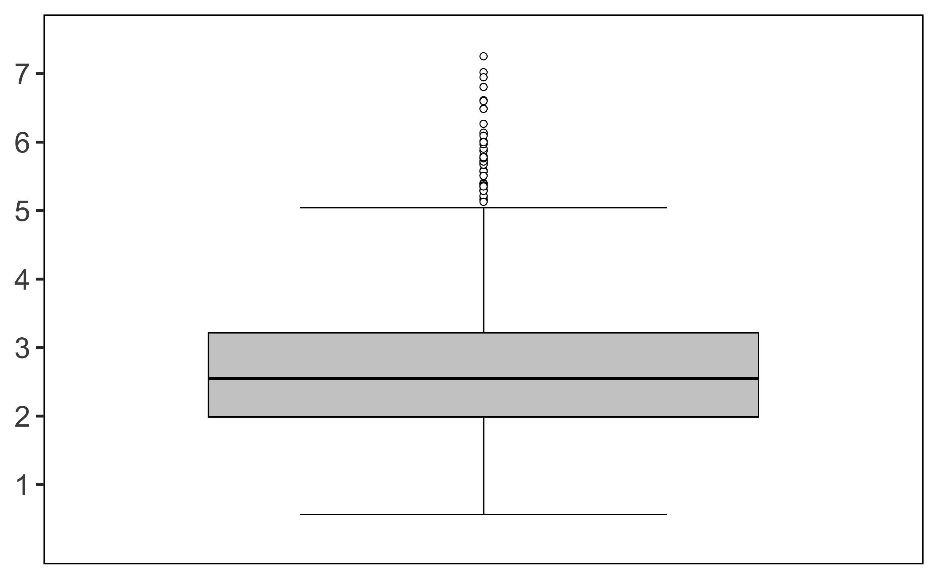
We begin by evaluating whether the Gini mean difference of the income-to-hours ratio (INCTOT/UHRSWORK) is homogeneous across counties. This measure serves as a proxy for effective hourly pay and may reveal whether income disparities vary significantly across regions. The estimated GMDs range from 0.56 to 7.25. Figure 2 displays their distribution across counties.
At this point, we apply the resampling methodology described in Subsection 6.2. In Table 5, we report results for values of ranging from 5 to 40 in increments of 5 and for .
| Test | |||||||||
| 10 | N | ||||||||
| LB | 0.03 | 0 | 0.40 | 0 | 0 | 0 | 0 | 0 | |
| 20 | N | ||||||||
| LB | 0.22 | 0 | 0 | 0 | 0 | 0 | 0 | 0 | |
| 30 | N | ||||||||
| LB | 0 | 0 | 0 | 0 | 0 | 0 | 0 | 0 | |
| 40 | N | ||||||||
| LB | 0 | 0 | 0 | 0 | 0 | 0 | 0 | 0 | |
| 50 | N | ||||||||
| LB | 0 | 0 | 0 | 0 | 0 | 0 | 0 | 0 |
Table 5 shows that for and , the test consistently rejects the null hypothesis, with associated -values being extremely small. Moreover, for , the decision is stable across all considered values of . This observation is consistent with the results in Section 7: under alternatives, the power increases with , while under the null, the level is only slightly affected by the choice of . Altogether, the results provide strong evidence against the null hypothesis and support the practical adequacy of using as an upper bound, as originally proposed in Cuesta-Albertos and Febrero-Bande, (2010).
Spearman’s correlation between working hours and earned income
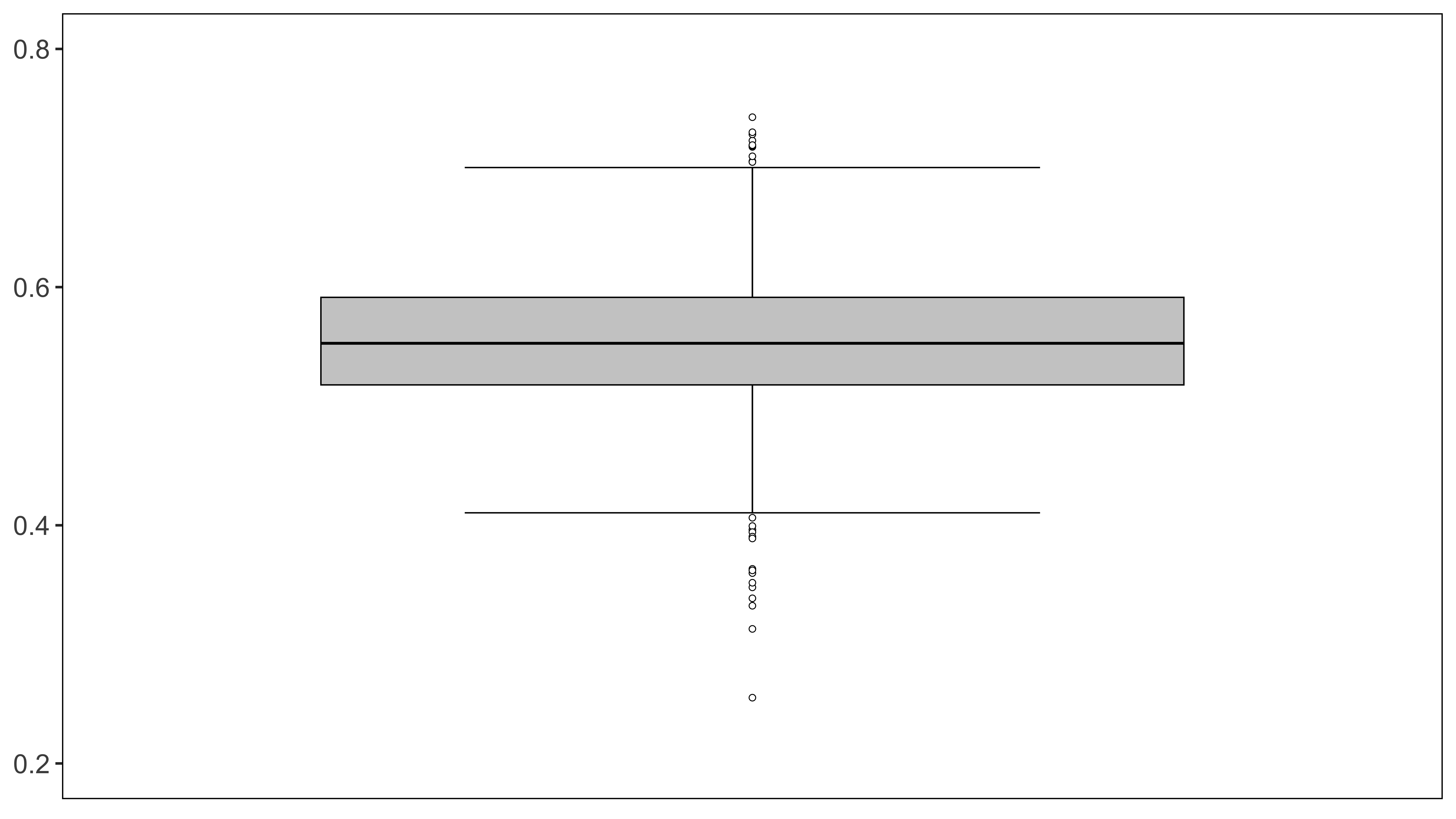
We analyze between the number of usual hours worked per week and earned income to assess the homogeneity of the relationship across all counties. The estimated Spearman’s rho are all positive, ranging from 0.26 to 0.74, indicating that in every county the two variables exhibit a positive association. The distribution of estimated is displayed in Figure 3.
As done in the previous case, we now perform the same resampling study. The resulting -values are presented in Table 6.
| Test | |||||||||
| 10 | N | 0.60 | 0.75 | 0.74 | 0.36 | 0.51 | 1 | 0.46 | 0.37 |
| LB | 0.90 | 1 | 1 | 1 | 1 | 1 | 1 | 1 | |
| 20 | N | 0.02 | 0.02 | ||||||
| LB | 0.40 | 0.19 | 0.12 | 0 | 0 | 0.78 | 0.25 | 0 | |
| 30 | N | ||||||||
| LB | 0.01 | 0.13 | 0 | 0 | 0 | 0 | 0 | 0 | |
| 40 | N | ||||||||
| LB | 0.18 | 0 | 0 | 0 | 0 | 0 | 0 | 0 | |
| 50 | N | ||||||||
| LB | 0 | 0 | 0 | 0 | 0 | 0 | 0 | 0 |
Looking at this table, we see that for and , the test consistently rejects the null, with low -values. Moreover, for , is rejected for every considered value of . In contrast, for , the test does not reject the null, even for large values of . These findings are in line with those discussed for the Gini case and more clearly highlight the influence of on the test decision, as previously noted. Taken together, the results provide strong evidence against the null in this setting.
9 Conclusions and future work
In this work, a general, nonparametric test based on –statistics was developed for assessing the equality of parameters across a large number of populations. Under mild moment and sample‐size comparability conditions, the proposed test statistic converges to a normal distribution under the null hypothesis. In addition, a ratio‐consistent estimator of its variance was provided, which, together with the statistic’s convergence, enables asymptotically exact inference without parametric assumptions. A linear bootstrap approximation to improve the performance for small to moderate , and a random sampling strategy to reduce computational burden, were also implemented. Simulation studies for the Gini mean difference and Spearman’s rho were conducted to examine the behavior of both the asymptotic and bootstrap versions in terms of Type I error control and power, across different group sizes and alternatives. A real-data application was also presented to illustrate the procedure.
A number of extensions are possible. In many real‐world settings the observations within each group may exhibit temporal or spatial dependence (for example, in time‐series or panel data), so extending the theory to accommodate dependent data is an important avenue for future work. Likewise, it is often of interest to compare vector‐valued or multivariate functionals, such as covariance matrices or other high‐dimensional summaries, across many populations. In this regard, generalizing the current framework to parameters of arbitrary dimension is therefore another line for future research.
10 Proofs
Throughout this section, denote generic positive constants that are not important and may vary from one step to another, or even between different occurrences within the same line of an inequality. A sequence of random variables is if it converges to 0, and is if it is bounded in probability.
Proof of Lemma 1.
Note that
We know that , , for . To prove the first part of the result it suffices to show
| (15) |
| (16) |
and
| (17) |
Firstly we prove (15) and (16). As the random variables (also ) are independent but not identically distributed we apply Kolmogorov’s Strong Law of Large Numbers (see Theorem D in Chapter 1.8 of Serfling, (1980)). To do so, it suffices to show that From (90) and (91), we have
| (18) |
An analogous equation holds for
| (19) |
where the last inequality follows from the independence of and .
Therefore, since we have (5), we obtain (15) and (16), which in turn implies convergence in probability. Finally, we proceed to prove (17). From (5) and (18), and observing that
| (20) |
it follows that , we get and then (17) is fulfilled.
For the second part, we only need to show that the convergence in (17) is almost sure. Note that
From (18), we know that , so to prove the result, it suffices to show that
To do so, we apply Corollary 3.9 of White, (2014), where we only need to check that , for some and all . Using the inequality, we get
| (21) |
Then, as for , the result is proven. ∎
Proof of Lemma 2.
To obtain the result, we follow a similar approach to that described in Section 3 of Akritas and Papadatos, (2004). In this case, the projection is applied by conditioning to the samples , rather than to the individual random variables. By applying the Decomposition Lemma of Efron and Stein, (1981) we get
| (22) |
Computing the conditional expectations, we find
and for
Substituting these expressions into (22), the result follows. ∎
Remark 2.
Note that can be expressed as the sum of and , where
| (23) | ||||
The term corresponds to a degree- -statistic with a symmetric kernel ,
where is defined in (3). We have that
since . Therefore is degenerated. Now, we compute the second order variance, i.e. . First, we calculate the conditional expectation
| (24) | ||||
where . Routine calculations show that
| (25) |
On the other hand,
| (26) |
Substituting (25) and (26) into (24), it follows that
and noting that,
we get
Since is degenerated, from (91), (9) and the previous equation, it follows that
| (27) |
On the other hand, using (90), (91) and (9), we obtain
| (28) |
By applying inequality we get
Furthermore, for the monotonicity of moments, we note that
| (29) |
In addition, from (19), we have
Substituting all the previous bounds into (28), we obtain
| (30) |
The term is a degree-2 -statistic whose kernel is given by
and then
| (31) |
This implies that, in general, is a non-degenerated -statistic, and then, for analogous reasons to , we have that
| (32) |
We also have an upper bound on . From (90), (91) and (9), we get
| (33) |
then, by inequality and (29), it follows that
and hence
| (34) |
Before proving Lemma 3, we first present some preliminary results. Throughout this work, by convention, we set the binomial coefficient as
| (35) |
In the following proof, we will make use of the identities provided in Section B of the appendix.
Lemma 6.
Proof.
First, from (93) we note that
| (36) |
In addition, we have that
| (37) |
Then, from the symmetry of the binomial coefficients and noting that the term for equals 0 since , we get that
Hence, using the last equation we can write
where we have changed the order of summations. Now applying property (93) twice, we get
Now we apply Vandermonde’s identity (94) yielding
| (38) |
where we have extended the sum to because if . Then, recalling the definition of in (91), we obtain the desired result.
∎
Lemma 7.
Proof.
We have
Since is symmetrically defined in its arguments we only need to compute
for fixed indices and multiply it by all the possible permutation of those. In the above expression, we have indices for the random variables, of which at least must be distinct. It is evident that any covariance involving distinct indices will be zero due to the independence of the random variables. Therefore, the non-zero terms will correspond to those in which , where ranges from to . Additionally, the value of these terms depends on the specific place where those indices are repeated in . Hence, if indices are repeated the non-zero terms, considering that all random variables are identically distributed, will be
| (40) |
Let be the number of ways in which indices can repeat, with of these indices appearing in the same configuration as in . With this notation we can write
| (41) |
In the following we calculate . There are ways of choosing indices from a set of . Fixing one choice of those , there are ways to choose elements from those and partition them into two groups of and elements. Once this is done, we need to count the ways of distributing them into those two groups. This can be done in the same ways of those of partitioning the remaining elements, i.e. ways. Finally we have to take into accunt the permutations of those elements. Thus,
| (42) |
and hence, from (42) and (41) we obtain
| (43) |
Now we write in terms of the centered kernel , defined in (87). Hence, defining
| (44) |
we can write
Now, using (89), we can identify the covariances above, yielding
| (45) |
Introducing (45) into (43), we get
where
| (46) |
From Lemma 6, and the result holds. ∎
Proof of Lemma 3.
Lemma 8.
Proof.
First, note that applying Cauchy-Schwarz inequality, we have that
where the last inequality follows from (90). In addition, we know that , which, from (5), is uniformly bounded, and hence
Now, as is a fixed quantity, it follows that all the binomial coefficients involving and are bounded. Note also that . Then we get
where the last equality follows from (9). Hence
since is a strictly decreasing function of in its domain , its maximum is attained at , where it takes the value . Thus, since we are considering finite values of , the result follows. ∎
Before proving Lemma 4 we introduce some useful bounds for .
Lemma 9.
Proof.
- 1.
- 2.
- 3.
-
4.
To establish the upper bound, we apply the inequality, which gives Using bound (30) and noting that is bounded, we obtain Similarly, from equation (33) and the fact that is uniformly bounded, we deduce that
which is bounded from (5). Combining these results, we conclude the upper bound on . To establish the lower bound, we consider (49) along with assumption 1.ii.
At this point myltiplying the previous inequality and recalling (8), we get
where the last inequality follows from . Since , the result holds for large .
-
5.
To get the lower bound, from Lemma 3 we have
∎
Proof of Lemma 4.
Note that,
| (53) |
where
So, to show the result it suffices to see that
| (54) |
for . We now upper-bound as follows:
| (55) |
where the third equality follows from the independence of samples. Specifically, the expectation
retains only terms where pairs of indices match, a situation that occurs twice, resulting in the expression (55).
At this stage, by appliying (91) and recalling (90) along with , we can obtain an upper bound on , given by
| (56) |
where the last inequality follows from Vandermonde’s identity (94). In addition, we have that
where the last inequality follows from (9). Substituting the previous equation into (56), we have that
| (57) |
and thus, from (55) we get the bound
| (58) |
Next, to study , we consider different cases.
- •
- •
Proof of Lemma 5.
To prove the result, we verify Lindeberg’s condition
| (63) |
where denotes the indicator function.
We proceed by analyzing different cases, starting with the assumption that holds. First, we multiply and divide by . Then, invoking the lower bound in (48), we obtain that, to prove (63), it suffices to show that
| (64) |
Next, observe that
Consequently, we obtain the bound
| (65) |
Since , from the upper bound in (48) it follows that is finite. Using this result and applying the Dominated Convergence Theorem to (65), we deduce that for each ,
Therefore, (63) holds when is true.
Now assume that Assumption 1.i holds. Recalling the lower bound in (50), it follows that, to establish (63), it suffices to verify that
From the lower bound in (50), it follows that
which yields
| (66) |
Once again, since , the upper bound in (50) implies that is bounded. This allows us to apply the Dominated Convergence Theorem to (66), which in turn confirms that (63) holds under Assumption 1.i.
Suppose now that Assumption 1.ii holds and that . From the lower bound in (51), it suffices to show that
In this case, from the lower bound in (51), we get
and then
| (67) |
As , from the upper bound in (51), . Hence, we apply the Dominated Convergence Theorem noting that since is positive and , for some , we have
Finally, we assume that Assumption 1.ii holds and that . Recalling the lower bound in (52), we conclude that, to establish (63), it suffices to verify that (64) holds. Now, from the upper bound in (52), we get that is finite. Following the same reasoning as in the first case, one gets that (63) holds. ∎
Proof of Theorem 1.
Proof of Proposition 1.
In first place, can be decomposed as
| (68) |
where
and for . By definition, and can be written as follows
| (69) |
As we are assuming (5), we have, as we saw in the proof of Lemma 1, that and hence
| (70) |
Similarly, as is finite under (5), it follows that
| (71) |
Now we check Lindeberg’s condition
| (72) |
Now, we observe that, from (10), is bounded away from zero, and thus is a non-degenerate -statistic. Therefore, from (91) and (9), we conclude that
| (73) |
and thus is bounded from below by some constant. Thus, to check Lindeberg’s condition it suffices to see that
Hence, considering the bound (73), it follows that
which implies
Now, as we showed in (57), as since (5) and (9) hold, we have that
Now, by applying the Dominated Convergence Theorem as in the proof of Lemma 5, we conclude that Lindeberg’s condition is satisfied. This implies that
| (74) |
where follows a standard normal distribution. Finally, since and from (74), we obtain that
| (75) |
Finally, from (70), (71) and (75), it follows that
Next, we are going to prove that .
First, it is important to note that (5) is sufficient to guarantee that is upper-bounded, as shown in Lemma 9. Consequently, is also upper-bounded.
-
•
If holds, from the lower bound in (48), since in this case , we have
for , because it is assumed that .
- •
- •
- •
On the other hand, and . Hence, can be expressed as
Lemma 5 establishes that, under either or Assumption 1,
As a consequence, it follows that
which further implies that
Finally, this leads to
We now compute
where we used that due to the independence of the random samples, along with the fact that . Now, from the bounds in Lemma 9, we get
| (76) |
since . Therefore, by applying Markov’s inequality, we obtain
We have proven that
| (77) |
Under , we apply Markov’s inequality, the inequality, and a refinement of the inequality from Theorem 2 of von Bahr (1965), obtaining
| (78) |
The last inequality follows from the upper bound in (48) and the assumption that is uniformly bounded. This establishes that
which, recalling the lower bound on in (48), implies
Thus, from (77), we conclude that under ,
| (79) |
If Assumption 1.i holds, recalling (50) and following a similar reasoning, we obtain that (79) holds. Otherwise, if Assumption 1.ii holds and is bounded, applying the bound (51), and noting that
proceeding analogously, we conclude that (79) also holds. In the case where Assumption 1.ii holds and , from the bounds in (52), and following the same steps as in the first case, (79) follows.
Proof.
The proof follows a similar argument to that of Lemma 7 in Jiménez-Gamero et al., (2025). ∎
Proof of Theorem 2.
First, the critical region is given by
From Theorem 1, under Assumption 1, we have that
On the other hand, from Proposition 1, we know that
where . With these results, the critical region can be written as
| (80) |
Now, we analyze the behavior of both sides of the inequality case by case:
-
a)
If Assumption 1.i holds, for the left-hand side of (80), recalling the upper-bound of (50), we have that
for either bounded or . To prove the result, it suffices to show that is upper-bounded, which reduces to establishing the same for . From Lemma 10, it is sufficient to verify that is upper-bounded, which is immediate from (20). Then, all the above implies that .
- b)
- c)
-
d)
If Assumption 1.ii holds, , , and , we express the critical region (80) as
For the left-hand side of the previous inequality, we get
where we have used the upper bound on obtained in (51). Sach a bound implies that Then, to prove the result, it suffices to check that This follows from Lemma 10, together with the bound stated in (8), and the assumption given in Proposition 1.
- e)
∎
Proof of Proposition 2.
Since , the power of the test is given by,
-
1.
First, note that since is fixed, by Lemma 9, . We also know, from Lemma 10, that . These arguments imply that , and hence
(82) Now, from (8) and the aforementioned bounds for , we have that
(83) As we are assuming that , from the monotonicity of the cumulative distribution function, it follows that . If additionally, , from (82) we obtain that .
-
2.
We proceed as in the first case. First, it is important to note that
Next, we study the term , recalling Lemma 10, (8), (52) and the equation above, we have that
(84) since we are assuming that is upper-bounded. Therefore (82) also holds in this case. In addition, we have that
Then, as we are assuming that , from the monotonicity of the cumulative distribution function, it follows that . If additionally, , from (82) we obtain that .
- 3.
Acknowledgements
This research has been financed by research project PID2022-137818OB-I00 (Ministerio de Ciencia, Innovación y Universidades, Spain).
References
- Akritas and Arnold, (2000) Akritas, M. G. and Arnold, S. F. (2000). Asymptotics for analysis of variance when the number of levels is large. Journal of the American Statistical Association, 95(449):212–226.
- Akritas and Papadatos, (2004) Akritas, M. G. and Papadatos, N. (2004). Heteroscedastic one-way anova and lack-of-fit tests. Journal of the American Statistical Association, 99(466):368–382.
- Alba-Fernández et al., (2024) Alba-Fernández, M., Jiménez-Gamero, M., and Jiménez-Jiménez, F. (2024). Testing for proportions when data are classified into a large number of groups. Mathematics and Computers in Simulation, 223:588–600.
- Bartlett, (1937) Bartlett, M. S. (1937). Properties of sufficiency and statistical tests. Proceedings of the Royal Society of London. Series A, 160:268–282.
- Bathke, (2002) Bathke, A. C. (2002). Anova for a large number of treatments. Mathematical Methods of Statistics, 11(1):118–132.
- Benjamini and Yekutieli, (2001) Benjamini, Y. and Yekutieli, D. (2001). The control of the false discovery rate in multiple testing under dependency. The Annals of Statistics, 29(4):1165–1188.
- Boos and Brownie, (1995) Boos, D. D. and Brownie, C. (1995). Anova and rank tests when the number of treatments is large. Statistics & Probability Letters, 23(2):183–191.
- Cuesta-Albertos and Febrero-Bande, (2010) Cuesta-Albertos, J. and Febrero-Bande, M. (2010). A simple multiway ANOVA for functional data. Test, 19(3):537–557.
- Efron and Stein, (1981) Efron, B. and Stein, C. (1981). The jackknife estimate of variance. The Annals of Statistics, 9(3):586–596.
- Fisher, (1925) Fisher, R. A. (1925). Statistical Methods for Research Workers. Oliver and Boyd, Edinburgh.
- Giacomini et al., (2013) Giacomini, R., Politis, D. N., and White, H. (2013). A warp-speed method for conducting monte carlo experiment involving bootstrap estimators. Econometric Theory, 29(3):567–589.
- Harrar and Bathke, (2008) Harrar, S. W. and Bathke, A. C. (2008). Nonparametric methods for unbalanced multivariate data and many factor levels. Journal of Multivariate Analysis, 99(8):1635–1664.
- Hoeffding, (1948) Hoeffding, W. (1948). A Class of Statistics with Asymptotically Normal Distribution. The Annals of Mathematical Statistics, 19(3):293 – 325.
- Jiménez-Gamero, (2024) Jiménez-Gamero, M. D. (2024). Testing normality of a large number of populations. Statistical Papers, 65:435–465.
- Jiménez-Gamero et al., (2022) Jiménez-Gamero, M. D., Cousido-Rocha, M., Alba-Fernández, M. V., et al. (2022). Testing the equality of a large number of populations. Test, 31:1–21.
- Jiménez-Gamero and de Uña Álvarez, (2024) Jiménez-Gamero, M. D. and de Uña Álvarez, J. (2024). Testing poissonity of a large number of populations. Test, 33:1863–8260.
- Jiménez-Gamero et al., (2025) Jiménez-Gamero, M. D., Valdora, M., and Rodríguez, D. (2025). Testing homoscedasticity of a large number of populations. Statistical Papers, 66(1):32.
- Kim, (2021) Kim, I. (2021). Comparing a large number of multivariate distributions. Bernoulli, 27(1):419 – 441.
- Kruskal and Wallis, (1952) Kruskal, W. H. and Wallis, W. A. (1952). Use of ranks in one-criterion variance analysis. Journal of the American Statistical Association, 47(260):583–621.
- Lee, (1990) Lee, A. J. (1990). U-Statistics: Theory and Practice. Marcel Dekker.
- Levene, (1960) Levene, H. (1960). Robust tests for equality of variances. In Olkin, I. e. a., editor, Contributions to Probability and Statistics: Essays in Honor of Harold Hotelling, pages 278–292. Stanford University Press, Palo Alto, CA.
- Li and Yao, (2019) Li, D. and Yao, Q. (2019). Asymptotic tests for high-dimensional regression coefficients with heteroscedasticity. Journal of the Royal Statistical Society: Series B, 81(2):337–360.
- Maache and Lepage, (2003) Maache, H. E. and Lepage, Y. (2003). Spearman’s rho and Kendall’s tau for multivariate data sets. Lecture Notes-Monograph Series, 42:113–130.
- Rizzo and Székely, (2010) Rizzo, M. L. and Székely, G. J. (2010). Disco analysis: A nonparametric extension of analysis of variance. The Annals of Applied Statistics, 4(2):1034–1055.
- Ruggles et al., (2025) Ruggles, S., Flood, S., Sobek, M., Backman, D., Cooper, G., Drew, J. A. R., Richards, S., Rodgers, R., Schroeder, J., and Williams, K. C. W. (2025). IPUMS USA: Version 16.0 [dataset].
- Scholz and Stephens, (1987) Scholz, F. W. and Stephens, M. A. (1987). K-sample Anderson-Darling tests. Journal of the American Statistical Association, 82(399):918–924.
- Sen, (1974) Sen, P. K. (1974). Weak convergence of generalized -statistics. The Annals of Probability, 2(1):90–102.
- Serfling, (1980) Serfling, R. J. (1980). Approximation Theorems of Mathematical Statistics. Wiley, New York.
- von Bahr and Esseen, (1965) von Bahr, B. and Esseen, C.-G. (1965). Inequalities for the th absolute moment of a sum of random variables, . The Annals of Statistics, 36(6):299–303.
- White, (2014) White, H. (2014). Asymptotic theory for econometricians. Academic press.
- Zhan and Hart, (2014) Zhan, D. and Hart, J. D. (2014). Testing equality of a large number of densities. Biometrika, 101(2):449–464.
Appendix A Classical Results on U-Statistics
In this section, we present some properties of U-statistics, which will be instrumental in proving the main results later in the paper. The results and definitions not explicitly referenced can be found in Sections 5.1 and 5.2 of Serfling, (1980).
Let be a symmetric kernel of degree . Let be a random sample with . The U-statistic based on and the random sample is defined as
| (85) |
We say that is a degree- U-statistic. Let . The U-statistic is a symmetric function of its inputs and serves as an unbiased estimator of , i.e.,
To compute the variance of , we first define the conditional expectation of the kernel given variables
| (86) |
We define the centered version of as
| (87) |
Note that, . The variance of both and is
| (88) |
We also have that for indices and sharing exactly common elements, , where denotes the cardinality of ,
| (89) |
Note that the previous equation is valid if we replace the kernels for their centered version as well. The variances satisfy the ordering,
| (90) |
Using these variances, the variance of is given by
| (91) |
Appendix B Binomial coefficient properties
We summarize essential properties of binomial coefficients.
Identity B.1 (Symmetry)
| (92) |
Identity B.2
| (93) |
Identity B.3 (Vandermonde’s Identity)
| (94) |