Construction of optimal tests for symmetry on the torus and their quantitative error bounds

Abstract

In this paper, we develop optimal tests for symmetry on the hyper-dimensional torus, leveraging Le Cam’s methodology. We address both scenarios where the center of symmetry is known and where it is unknown. These tests are not only valid under a given parametric hypothesis but also under a very broad class of symmetric distributions. The asymptotic behavior of the proposed tests is studied both under the null hypothesis and local alternatives, and we derive quantitative bounds on the distributional distance between the exact (unknown) distribution of the test statistic and its asymptotic counterpart using Stein’s method. The finite-sample performance of the tests is evaluated through simulation studies, and their practical utility is demonstrated via an application to protein folding data. Additionally, we establish a broadly applicable result on the quadratic mean differentiability of functions, a key property underpinning the use of Le Cam’s approach.

Abstract

Section S1 of this supplement contains the proofs of all propositions, theorems and lemmas of the main paper. Some further simulation results can be found in Section S2.

Keywords Asymptotic theory $\cdot$ Directional statistics $\cdot$ Le Cam’s theory $\cdot$ Protein folding $\cdot$ Quadratic mean differentiability $\cdot$ Stein’s method

1 Introduction

Various complex data obtained from the real world can be viewed as data on the $d$-dimensional torus, which is the cartesian product of $d$ circles. Concrete examples include wind direction measured at different times during the day (johnson_measures_1977 ; kato_distribution_2009 ; shieh_inferences_2005 ), directions of steepest descent before and after an earthquake (rivest_decentred_1997 ), direction of animal movement (mastrantonio_modelling_2022 ), shared orthologous genes between circular genomes (fernandez-duran_modeling_2014 ), morphological data from human neurons (puerta_regularized_2015 ) and, in marine biology, the spawning time of a particular fish and the time of the low tide (kato_circularcircular_2008 ). A domain that has given rise in the past two decades to a lot of such toroidal data is bioinformatics, where dihedral angles from proteins can be viewed as data on the torus, see kato2024versatiletrivariatewrappedcauchy ; kato_mobius_2015 ; mardia_multivariate_2008 ; mardia_mixtures_2012 ; mardia_protein_2007 ; singh_probabilistic_2002 , and these angles play an essential role in the protein structure prediction problem. Other examples from bioinformatics are RNA data (nodehi_estimation_2018 ) and the circadian clock of two different tissues of a mouse (liu_phase_2006 ).

In the literature there exist a lot of distributions for data on the (hyper-)torus. Firstly, for one angle, meaning circular data, there is an abundance of literature proposing models, see for example mardia_directional_2000 for an overview. The most classical distributions are the von Mises distribution, which arises as a maximum entropy distribution, the wrapped Cauchy, the cardioid, and the wrapped Normal. Distributions for two angles include the bivariate von Mises distribution (mardia_statistics_1975 ), its submodels, which are the Sine (singh_probabilistic_2002 ) and Cosine (mardia_protein_2007 ) distributions, and the bivariate wrapped Cauchy distribution (kato_mobius_2015 ; kato_distribution_2009 ). The trivariate wrapped Cauchy copula (TWCC) (kato2024versatiletrivariatewrappedcauchy ) can model three angles, while the multivariate von Mises (mardia_multivariate_2008 ), multivariate wrapped normal (Baba1981 ) and the multivariate non-negative trigonometric sums (MNNTS) (fernandez-duran_modeling_2014 ) models can be used for any dimension.

All aforementioned distributions, except the MNNTS, are symmetric models. However, many datasets involve skewed data. In order to overcome this shortcoming of flexible asymmetric models, ameijeiras-alonso_sine-skewed_2022 proposed the sine-skewed family of distributions, building on the work of umbach_building_2009 ; abe_sine-skewed_2011 which skewed one-dimensional circular distributions. The proposed transformation, given in (1), can turn any symmetric distribution, of any dimension, into an asymmetric one and has several attractive properties, such as unchanged normalizing constant, easy interpretation and simple data generating mechanism. Thanks to these attractive properties, the sine-skewed construction, in particular in combination with the Sine model, has been implemented in the probabilistic programming languages Pyro and NumPyro (ronning_time_efficient_2021 ). This sine-skewing construction raises the following question: when should the simpler symmetric distribution be used and when should the more complicated, yet more flexible skewed version of it be preferred? This question was partly answered in ameijeiras-alonso_sine-skewed_2022 , using likelihood ratio tests. However, these parametric tests are not enough for an informed decision whether the dataset is symmetric or not. Generally valid tests are needed to better understand the data without any restrictive parametric assumptions. For dimension $d=1$, optimal tests are proposed by ameijeiras-alonso_optimal_2021 ; ley_simple_2014 for the cases of known and unknown symmetry center, respectively. The goal of this paper is to derive tests for symmetry for $d$-dimensional toroidal data that are robust to the assumption of the underlying distribution of the data, for both known and unknown symmetry centers. Moreover, we wish our tests to be efficient against the class of sine-skewed alternatives.

In order to reach our goals we develop the Le Cam theory of asymptotic experiments le2012asymptotic for hyper-toroidal settings, and optimality is to be understood in the Le Cam sense, namely asymptotically (in the sample size) and locally (against local sine-skewed deviations from symmetry). In particular, we will establish the Uniform Local Asymptotic Normality (ULAN) property for a broad class of symmetric distributions on the hyper-torus. For both known and unknown center scenarios, we start by constructing optimal parametric tests under a specified symmetric distribution, which we will then turn into semi-parametric tests that are valid under a very broad class of symmetric distributions on the torus satisfying mild regularity conditions. Each resulting semiparametric test will not only be robust to the assumption of the underlying distribution but moreover remain optimal under the parametric distribution it was built. Moreover, when the center of symmetry is known, all tests are exactly of the same form, leading to a single test that is uniformly optimal to test symmetry against sine-skewed distributions. This is a very powerful and quite rare result. The tests are easy to compute numerically, with their computational complexity increasing with the dimension of the data set and the difficulty of inverting the corresponding Fisher Information matrix, which is $O(d^{3})$ for a $d\times d$ matrix (trefethen2022numerical ), as well as the sample size. More specifically, the computational complexity of the algorithm in the case of the specified symmetry center case is $O(n^{2}d^{9})$, where $d$ is the dimension of the problem and $n$ is the sample size of the dataset under consideration. In the case of the unspecified symmetry center, it becomes $O(n^{6}d^{23})$.

Since the rejection rules of our new tests will be based on their asymptotic distribution, there will inevitably be approximation errors as real data naturally have a finite sample size. The larger this sample size, the smaller the approximation error between the intractable exact distribution of our test statistics and their simple asymptotic law. This is a reality for the overwhelming majority of existing hypothesis testing procedures. Unlike most of the literature, in this paper we wish to quantify this approximation error, and we will tackle this difficult problem through the suit of several technical calculations and proofs. One part of our proofs will rely on Stein’s Method, which is an important tool in applied and theoretical probability, whose principal aim is to provide quantitative assessments in distributional approximation problems of the form $W\approx Z$, where $Z$ follows a simple distribution and $W$ is the object of interest (stein1972bound ). Stein’s Method is known to be effective for numerous approximation problems, including the normal, the Poisson, the exponential and the Beta, among many others (ley_reinert_swan2017 ; ross_stein2011 ). It has successively been used to assess approximation errors for maximum likelihood estimators (anastasiou2017bounds , anastasiou2017_MLE_m , anastasiou2018_MLE , anastasiou_gaunt2021 ), the likelihood ratio statistic (reinert_anastasiou2020 ), Pearson’s chi-square statistic (gaunt_pickett_reinert2017 ), Friedman’s statistic (gaunt_reinert_Friedman2023 ), and neural networks (favaro_quantitative_2025 ), to name but a few. For a general overview, we refer the reader to anastasiou_stein2023 .

The novelty of our paper does not just arise from defining symmetry tests for the first time on the torus. It is also, to the best of our knowledge, the first paper that combines Le Cam’s theory of asymptotic experiments and Stein’s Method in the context of optimal testing for symmetry. Moreover, in Proposition 1, we provide a general result for quadratic mean differentiability of products of functions, a necessary condition for the ULAN property to be proved for our setting but which also applies to many other settings from the literature. Hence, besides recovering various existing results from the literature, this proposition also paves the way for establishing ULAN in future papers for many distinct settings since quadratic mean differentiability is often a main difficulty in establishing ULAN. Finally, our paper is the first statistical confirmation that dihedral angles from proteins are asymmetric, which provides further insights in the structure of the proteins.

The outline of the paper is as follows. In Section 2, through Proposition 1, we establish the ULAN property of the family of sine-skewed distributions, as defined in (1). In Sections 3 and 4, we respectively propose optimal tests for symmetry on the $d$-dimensional torus in the cases that the symmetry center is known or unknown and needs to be estimated. The theoretical properties of both tests are investigated, including the asymptotic distribution under the null hypothesis of symmetry, which turns out to be chi-squared with $d$ degrees of freedom, and under local alternatives, which is non-central chi-squared with $d$ degrees of freedom, where $d$ is the dimensionality of the problem. Bounds between the complicated finite-sample distribution of the test statistics and their simple limiting distributions are derived using Stein’s Method. Extensive numerical simulations, as well as a real data application using protein folding data can be found in Sections 5 and 6, respectively. Section 7 concludes the paper with a summary of the most important findings. The supplementary material contains all proofs of the theorems and lemmas presented in the main paper, along with some further results that are used for the proofs, as well as some further simulation results. The implementation of the tests can be found in https://doi.org/10.5281/zenodo.17224138 and https://github.com/Sophia-Loizidou/Symmetry_test_on_hypertorus.

2 Family of distributions and the ULAN property

2.1 A technical result about Quadratic Mean Differentiability

A common analytical condition in order to establish a ULAN property is quadratic mean differentiability (QMD) of the square root of densities (see Section 2.3 for details in our context). Since sine-skewed densities correspond to a product or composition of two functions, we provide in this section a general statement for the QMD property under function composition. This result goes beyond the mere setting of this paper and actually holds for very general settings. We therefore also consider a general support $\mathbb{R}^{m}$ for the pdfs. The proof can be found in Section S1.1 of the supplementary material. For the proposition, and the rest of the paper, we denote the usual supremum norm of a function $\lVert h\rVert=\lVert h\rVert_{\infty}=\sup_{x\in\mathbb{R}}|h(x)|$.

Proposition 1.

Consider the functions $f(\boldsymbol{x};\boldsymbol{\mu}),g(\boldsymbol{x};\boldsymbol{\mu},\boldsymbol{\lambda})$, $f,g:\mathcal{X}\subset\mathbb{R}^{m}\rightarrow\mathbb{R}^{+}$ with parameters $\boldsymbol{\mu}\in\mathbb{R}^{k},\boldsymbol{\lambda}\in\mathbb{R}^{m}$. Assume that $f(\boldsymbol{x};\boldsymbol{\mu})$ and $f(\boldsymbol{x};\boldsymbol{\mu})g(\boldsymbol{x};\boldsymbol{\mu},\boldsymbol{\lambda})$ are probability density functions and that $f$ and $g$ satisfy the following conditions:

1. $g(\boldsymbol{x};\boldsymbol{\mu},\boldsymbol{\lambda})$ is almost everywhere (a.e.) $\mathcal{C}^{1}$ over $\mathcal{X}$ with respect to $\boldsymbol{\lambda}$;

2. $||\nabla_{\boldsymbol{\lambda}}g^{1/2}(\boldsymbol{x};\boldsymbol{\mu},\boldsymbol{\lambda})|_{\boldsymbol{\lambda}=0}||\leq C\ell(\boldsymbol{x};\boldsymbol{\mu})$ for some $C\in\mathbb{R}^{+}$ independent of both $\boldsymbol{\mu},\boldsymbol{\lambda}$ and some function $\ell(\boldsymbol{x};\boldsymbol{\mu})$ that is in $L^{2}(f(\boldsymbol{x};\boldsymbol{\mu})d\boldsymbol{x})$;

3. $f(\boldsymbol{x};\boldsymbol{\mu}),g(\boldsymbol{x};\boldsymbol{\mu},\boldsymbol{\lambda})>0$ a.e. over $\mathcal{X}$;

4. $g(\boldsymbol{x};\boldsymbol{\mu},\boldsymbol{0})=1$ and $\nabla_{\boldsymbol{\mu}}g(\boldsymbol{x};\boldsymbol{\mu},\boldsymbol{\lambda})|_{\boldsymbol{\lambda}=0}=0$;

5. For $\boldsymbol{\mu}=(\mu_{1},\ldots,\mu_{k})^{\prime}$ and $i\in\{1,\ldots,k\}$, $\int_{\mathcal{X}}\left(\frac{\partial}{\partial_{\mu_{i}}}f^{1/2}(\boldsymbol{x};\boldsymbol{\mu})\right)^{2}{\mathrm{d}}\boldsymbol{x}<\infty$;

6. For $\boldsymbol{\lambda}=(\lambda_{1},\ldots,\lambda_{m})^{\prime}$ and $j\in\{1,\ldots,m\}$, $\int_{\mathcal{X}}\left(\frac{\partial}{\partial_{\lambda_{j}}}g^{1/2}(\boldsymbol{x};\boldsymbol{\mu},\boldsymbol{\lambda})|_{\boldsymbol{\lambda}=0}\right)^{2}f(\boldsymbol{x};\boldsymbol{\mu}){\mathrm{d}}\boldsymbol{x}<\infty$.

Then $f(\boldsymbol{x};\boldsymbol{\mu})$ is QMD with quadratic mean $\nabla_{\boldsymbol{\mu}}f^{1/2}(\boldsymbol{x};\boldsymbol{\mu})$ if and only if $f(\boldsymbol{x};\boldsymbol{\mu})g(\boldsymbol{x};\boldsymbol{\mu},\boldsymbol{\lambda})$ is QMD at $\boldsymbol{\lambda}=0$ with quadratic mean $\begin{pmatrix}\nabla_{\boldsymbol{\mu}}f^{1/2}(\boldsymbol{x};\boldsymbol{\mu})\\ f^{1/2}(\boldsymbol{x};\boldsymbol{\mu})\nabla_{\boldsymbol{\lambda}}g^{1/2}(\boldsymbol{x};\boldsymbol{\mu},\boldsymbol{\lambda})|_{\scriptscriptstyle\lambda=0}\end{pmatrix}$.

In order to avoid any confusion, we note that we denote by QMD both ‘quadratic mean differentiability’ and ‘quadratic mean differentiable’. Proposition 1 is very powerful as it gives a general proof for such modulated distributions on $\mathbb{R}^{m}$ (to the best of our knowledge, this terminology goes back to JUPP2016107 ). It retrieves in a single sweep several QMD results established in the literature for such distributions, for instance in the circular case for testing symmetry against $k$-sine-skewed alternatives in Theorem 2.1 of ley_simple_2014 , in the spherical case for testing rotational symmetry against skew-rotationally-symmetric alternatives in Theorem 1 of ley2017skew , in the multivariate Euclidean setting for testing elliptical symmetry against skew-elliptical alternatives in Theorem 2.1 of babic2021optimal (under some mild regularity assumption on their skewing function $\Pi$), to cite but these. Our result is also directly applicable for a range of modulated distribution models such as weighted distributions (see nakhaei2025weighting and references therein), cosine perturbation on the circle (abe2011symmetric ), etc. Since QMD is at the core of the ULAN property, Proposition 1 not only retrieves results from the literature but paves the way to obtain quite immediately ULAN results for modulated distributions and, hence, avoids an ad hoc proof in each case. Finally, note that in Assumption (ii) of Proposition 1 the function $\ell(\boldsymbol{x};\boldsymbol{\mu})$ can coincide with 1 when the support of the density is bounded, as will be the case for the family of sine-skewed distributions we describe next.

2.2 Family of sine-skewed distributions

As already mentioned in Section 1, the family of distributions we are interested in was proposed by ameijeiras-alonso_sine-skewed_2022 . For a $d-$dimensional angular vector $\boldsymbol{\theta}\in[-\pi,\pi)^{d}$, we consider sine-skewed densities of the form

$$\boldsymbol{\theta}\mapsto f_{\boldsymbol{\mu},\boldsymbol{\lambda}}(\boldsymbol{\theta};\boldsymbol{\Upsilon}):=f_{0}(\boldsymbol{\theta}-\boldsymbol{\mu};\boldsymbol{\Upsilon})\left(1+\sum_{j=1}^{d}\lambda_{j}\sin(\theta_{j}-\mu_{j})\right)\quad\mbox{subject to}\,\,\sum_{j=1}^{d}|\lambda_{j}|\leq 1,$$ (1)

where $\boldsymbol{\mu}\in[-\pi,\pi)^{d}$ is the hyper-toroidal location parameter, $\boldsymbol{\lambda}\in\mathbb{R}^{d}$ the skewness parameter, and $f_{0}$ is any symmetric density on the $d$-dimensional torus with $\boldsymbol{\Upsilon}$ the corresponding set of non-location parameters. We introduce the notation $S^{d}:=\left\{\boldsymbol{\lambda}\in\mathbb{R}^{d}\,\mbox{such that}\,\sum_{j=1}^{d}|\lambda_{j}|\leq 1\right\}$ for the domain of the skewness parameter. For the sake of readability, we will omit writing $\boldsymbol{\Upsilon}$ in the developments that follow. In this paper, we require $f_{0}$ to be a component-wise $2\pi$-periodic, unimodal, symmetric density, ensuring that the symmetry center $\boldsymbol{\mu}$ is uniquely defined. More formally, we require $f_{0}\in\mathcal{F}$, where $\mathcal{F}$ is defined as

$$\mathcal{F}:=\left\{\begin{array}[]{ll}&f_{0}(\boldsymbol{\theta})>0\,\mbox{a.e.}\,\ \forall\boldsymbol{\theta}\in[-\pi,\pi)^{d},\\ &f_{0}(\theta_{1}+2\pi k_{1},\ldots,\theta_{d}+2\pi k_{d})=f_{0}(\theta_{1},\ldots,\theta_{d})\ \forall k_{i}\in\mathbb{Z},i=1,\ldots,d,\\ f_{0}(\boldsymbol{\theta}):&f_{0}(\boldsymbol{\theta})=f_{0}(-\boldsymbol{\theta})\ \forall\boldsymbol{\theta}\in[-\pi,\pi)^{d},\\ &f_{0}\text{ unimodal in }\boldsymbol{\theta}\in[-\pi,\pi)^{d}\text{ with a mode at }\boldsymbol{0},\\ &\int_{[-\pi,\pi)^{d}}f_{0}(\boldsymbol{\theta}){\mathrm{d}}\boldsymbol{\theta}=1.\end{array}\right\}.$$ (7)

Most known models from the literature, such as the Sine, Cosine, bivariate wrapped Cauchy, trivariate wrapped Cauchy with specified marginals, or the multivariate von Mises, satisfy this requirement under certain restrictions on the parameter space to ensure unimodality. Whenever $\boldsymbol{\lambda}=\boldsymbol{0}$, we retrieve the original symmetric density $f_{0}$, otherwise the resulting density is sine-skewed. This naturally leads us to test the null hypothesis $\boldsymbol{\lambda}=\boldsymbol{0}$ against $\boldsymbol{\lambda}\neq\boldsymbol{0}$. Depending on whether the center of symmetry is known and on whether we assume $f_{0}$ to be known or not, we will have a distinct notation for the hypothesis testing problem, which we will introduce in Sections 3 and 4.

2.3 ULAN property

As already mentioned, we are interested in the symmetry hypothesis testing problem, that is, testing the null hypothesis $\boldsymbol{\lambda}=\boldsymbol{0}$ against the alternative $\boldsymbol{\lambda}\neq\boldsymbol{0}$. We derive four tests, depending on what we consider to be a nuisance parameter. Parametric tests are derived in the cases that the symmetry center is known (no nuisance parameters) and unknown ($\boldsymbol{\mu}$ is a nuisance parameter). Similarly, semi-parametric tests are also derived, when the symmetry center is known ($f_{0}$ is a nuisance parameter) and unknown (both $f_{0}$ and $\boldsymbol{\mu}$ are nuisance parameters).

We denote by $P^{(n)}_{\boldsymbol{\mu},\boldsymbol{\lambda};f_{0}}$, with $f_{0}\in\mathcal{F}$ as in (7), the joint distribution of a sequence $\{\boldsymbol{\theta}_{i}\}_{i=1}^{n}=\{(\theta_{1i},\ldots,\theta_{di})^{\prime}\}_{i=1}^{n}$ of independent and identically distributed (iid) hyper-toroidal random observations with density (1). Any $f_{0}$ then induces a toroidal location-skewness model

$$P^{(n)}_{f_{0}}:=\left\{P^{(n)}_{\boldsymbol{\mu},\boldsymbol{\lambda};f_{0}}:\boldsymbol{\mu}\in[-\pi,\pi)^{d},\boldsymbol{\lambda}\in S^{d}\right\}.$$

In order to derive tests for symmetry that are optimal in the Le Cam sense, we will establish the ULAN property in the vicinity of symmetry, meaning at $\boldsymbol{\lambda}=\boldsymbol{0}$, of the parametric model $P^{(n)}_{f_{0}}$. The ULAN property means that the distributions not only enjoy the local asymptotic normality (LAN) property, but also asymptotic linearity. For the ULAN property, we require the following mild assumption which is related to our general proposition from Section 2.1.

Assumption 1.a.

The mapping $\boldsymbol{\theta}\mapsto f_{0}^{1/2}\left(\boldsymbol{\theta}\right)$ is QMD over $\left[-\pi,\pi\right)^{d}$ with quadratic mean or weak vector derivative $({f_{0}^{1/2})}\dot{}\left(\boldsymbol{\theta}\right)$ and, letting ${\boldsymbol{\psi}}^{f_{0}}(\boldsymbol{\theta})=-2\frac{(f_{0}^{1/2})\dot{}\left(\boldsymbol{\theta}\right)}{f_{0}^{1/2}\left(\boldsymbol{\theta}\right)}$, the Fisher information matrix for location ${\boldsymbol{I}}^{f_{0}}_{\boldsymbol{\mu}\boldsymbol{\mu}}=\int_{[-\pi,\pi)^{d}}{\boldsymbol{\psi}}^{f_{0}}(\boldsymbol{\theta})({\boldsymbol{\psi}}^{f_{0}}(\boldsymbol{\theta}))^{\prime}f_{0}\left(\boldsymbol{\theta}\right){\mathrm{d}}\boldsymbol{\theta}$ has finite elements.

All our subsequent developments work under this mild assumption of weak differentiability. However, in view of notational simplicity and since all existing models from the literature actually possess regular derivatives, we shall henceforth work under the slightly stronger Assumption 1.b below.

Assumption 1.b.

The mapping $\boldsymbol{\theta}\mapsto f_{0}^{1/2}\left(\boldsymbol{\theta}\right)$ is continuously differentiable over $\left[-\pi,\pi\right)^{d}$ with continuous derivative

$$\nabla_{\boldsymbol{\mu}}f^{1/2}_{0}\left(\boldsymbol{\theta}-\boldsymbol{\mu}\right)=\begin{pmatrix}\frac{\frac{\partial}{\partial\mu_{1}}f_{0}\left(\boldsymbol{\theta}-\boldsymbol{\mu}\right)}{2f^{1/2}_{0}\left(\boldsymbol{\theta}-\boldsymbol{\mu}\right)}\\ \vdots\\ \frac{\frac{\partial}{\partial\mu_{d}}f_{0}\left(\boldsymbol{\theta}-\boldsymbol{\mu}\right)}{2f^{1/2}_{0}\left(\boldsymbol{\theta}-\boldsymbol{\mu}\right)}\end{pmatrix}=\frac{1}{2}\begin{pmatrix}\phi^{f_{0}}_{1}(\boldsymbol{\theta}-\boldsymbol{\mu})\\ \vdots\\ \phi^{f_{0}}_{d}(\boldsymbol{\theta}-\boldsymbol{\mu})\end{pmatrix}f^{1/2}_{0}\left(\boldsymbol{\theta}-\boldsymbol{\mu}\right),$$

where

$$\phi^{f_{0}}_{j}(\boldsymbol{\theta}-\boldsymbol{\mu})=-\frac{\frac{\partial}{\partial\theta_{j}}f_{0}(\boldsymbol{\theta}-\boldsymbol{\mu})}{f_{0}(\boldsymbol{\theta}-\boldsymbol{\mu})},\textrm{ for }j\in\{1,\ldots,d\}.$$ (8)

From Theorem 12.2.2 of lehmann_quadratic_2005 , quadratic mean differentiability of $\boldsymbol{\theta}\mapsto f_{0}^{1/2}\left(\boldsymbol{\theta}\right)$ is implied by continuous differentiability. Note that ${\psi}^{f_{0}}_{i}(\boldsymbol{\theta})$ in Assumption 1.a simplifies to $\phi^{f_{0}}_{i}(\boldsymbol{\theta})$ under Assumption 1.b. Moreover, the Fisher Information elements $I^{f_{0}}_{\mu_{i}\mu_{i}}=\int_{[-\pi,\pi)^{d}}\left(\phi^{f_{0}}_{i}(\boldsymbol{\theta})\right)^{2}f_{0}\left(\boldsymbol{\theta}\right){\mathrm{d}}\boldsymbol{\theta}$ are finite for $i\in\{1,\ldots,d\}$ by the assumption of continuous differentiability over a bounded domain. As already said, all known models from the literature satisfy Assumption 1.b. To avoid any misunderstandings, we provide a general definition of QMD in Definition 1 of the supplementary material. In view of the latter, it becomes clear that Assumption 1.b leads to quadratic mean differentiability of $P^{(n)}_{f_{0}}$ with respect to the location parameter at $\boldsymbol{\lambda}=\boldsymbol{0}$. As we shall see in the proof of Proposition 2, we need to establish QMD with respect to both location and skewness parameters to obtain the ULAN property. This will be a direct consequence of our general Proposition 1.

Let $\boldsymbol{\vartheta}=(\boldsymbol{\mu}^{\prime},\boldsymbol{\lambda}^{\prime})^{\prime}$ and $\boldsymbol{\vartheta}_{0}=(\boldsymbol{\mu}^{\prime},\boldsymbol{0}^{\prime})^{\prime}$. We now state the ULAN property of the family $P^{(n)}_{f_{0}}$ in the vicinity of symmetry, that is, at $\boldsymbol{\vartheta}_{0}$.

Proposition 2.

Let $f_{0}\in\mathcal{F}$ satisfy Assumption 1.b. Then the sine-skewed family $P^{(n)}_{f_{0}}$ is ULAN at $\boldsymbol{\vartheta}_{0}$. More precisely, for any $\mu_{i}^{(n)}=\mu_{i}+O(n^{-1/2}),i=1,\ldots,d,$ and for any bounded sequence $\boldsymbol{\tau}^{(n)}:=(\boldsymbol{\tau}^{(n)\prime}_{\mu},\boldsymbol{\tau}^{(n)\prime}_{\lambda})^{\prime}\in\mathbb{R}^{2d}$ with $\boldsymbol{\tau}^{(n)}_{\mu}=(\tau^{(n)}_{1},\ldots,\tau^{(n)}_{d})^{\prime}\in\mathbb{R}^{d}$, $\boldsymbol{\tau}^{(n)}_{\lambda}=(\tau^{(n)}_{d+1},\ldots,\tau^{(n)}_{2d})^{\prime}\in\mathbb{R}^{d}$ such that $\mu^{(n)}_{i}+n^{-1/2}\tau^{(n)}_{i}$, $i=1,\ldots,d,$ remains in $[-\pi,\pi)$, and $n^{-1/2}\tau^{(n)}_{j}\in[-1,1]$, $j=d+1,\dots,2d$ and $\sum_{j=d+1}^{2d}|\tau^{(n)}_{j}|<n^{1/2}$, we have

$$\Lambda^{(n)} :=\log\Biggl(\frac{P^{(n)}_{\boldsymbol{\mu}^{(n)}+n^{-1/2}\boldsymbol{\tau}^{(n)}_{\mu},n^{-1/2}\boldsymbol{\tau}^{(n)}_{\lambda};f_{0}}}{P^{(n)}_{\boldsymbol{\mu}^{(n)},\boldsymbol{0};f_{0}}}\Biggr)=\boldsymbol{\tau}^{(n)}{{}^{\prime}}\Delta_{f_{0}}^{(n)}(\boldsymbol{\mu}^{(n)})-\frac{1}{2}\boldsymbol{\tau}^{(n)}{{}^{\prime}}\Gamma_{f_{0}}\boldsymbol{\tau}^{(n)}+o_{P}(1)$$ (9)

as $n\to\infty$, and the central sequence

$$\Delta_{f_{0}}^{(n)}(\boldsymbol{\mu}):=\begin{pmatrix}\Delta_{f_{0};\mu}^{(n)}(\boldsymbol{\mu})\\ \Delta_{\lambda}^{(n)}(\boldsymbol{\mu})\end{pmatrix}=\frac{1}{\sqrt{n}}\sum_{i=1}^{n}\Delta_{f_{0};i}^{(n)}(\boldsymbol{\mu})=\frac{1}{\sqrt{n}}\sum_{i=1}^{n}\begin{pmatrix}\phi^{f_{0}}_{1}(\boldsymbol{\theta}_{i}-\boldsymbol{\mu})\\ \vdots\\ \phi^{f_{0}}_{d}(\boldsymbol{\theta}_{i}-\boldsymbol{\mu})\\ \sin(\theta_{1i}-\mu_{1})\\ \vdots\\ \sin(\theta_{di}-\mu_{d})\end{pmatrix},$$ (10)

for $\phi^{f_{0}}_{j}(\boldsymbol{\theta}-\boldsymbol{\mu})$ as in (8), converges to $\mathcal{N}_{2d}(\boldsymbol{0},\Gamma_{f_{0}})$ under $P^{(n)}_{\boldsymbol{\mu}^{(n)},\boldsymbol{0};f_{0}}$ as $n\to\infty$, where the Fisher information matrix $\Gamma_{f_{0}}$ is given by

$$\Gamma_{f_{0}}=\begin{pmatrix}I^{f_{0}}_{\mu_{1}\mu_{1}}&\ldots&I^{f_{0}}_{\mu_{1}\mu_{d}}&I^{f_{0}}_{\mu_{1}\lambda_{1}}&\ldots&I^{f_{0}}_{\mu_{1}\lambda_{d}}\\ \vdots&\ddots&\vdots&\vdots&\ddots&\vdots\\ I^{f_{0}}_{\mu_{1}\mu_{d}}&\ldots&I^{f_{0}}_{\mu_{d}\mu_{d}}&I^{f_{0}}_{\mu_{d}\lambda_{1}}&\ldots&I^{f_{0}}_{\mu_{d}\lambda_{d}}\\ I^{f_{0}}_{\mu_{1}\lambda_{1}}&\ldots&I^{f_{0}}_{\mu_{d}\lambda_{1}}&I^{f_{0}}_{\lambda_{1}\lambda_{1}}&\ldots&I^{f_{0}}_{\lambda_{1}\lambda_{d}}\\ \vdots&\ddots&\vdots&\vdots&\ddots&\vdots\\ I^{f_{0}}_{\mu_{1}\lambda_{d}}&\ldots&I^{f_{0}}_{\mu_{d}\lambda_{d}}&I^{f_{0}}_{\lambda_{1}\lambda_{d}}&\ldots&I^{f_{0}}_{\lambda_{d}\lambda_{d}}\end{pmatrix}$$ (11)

with

$$I^{f_{0}}_{\mu_{j}\mu_{k}}=\int_{[-\pi,\pi)^{d}}\phi_{j}^{f_{0}}(\boldsymbol{\theta})\phi_{k}^{f_{0}}(\boldsymbol{\theta})f_{0}(\boldsymbol{\theta}){\mathrm{d}}\boldsymbol{\theta},,\qquad I^{f_{0}}_{\lambda_{j}\lambda_{k}}=\int_{[-\pi,\pi)^{d}}\sin(\theta_{j})\sin(\theta_{k})f_{0}(\boldsymbol{\theta}){\mathrm{d}}\boldsymbol{\theta},$$

$$I^{f_{0}}_{\mu_{j}\lambda_{j}}=\int_{[-\pi,\pi)^{d}}\phi_{j}^{f_{0}}(\boldsymbol{\theta})\sin(\theta_{j})f_{0}(\boldsymbol{\theta}){\mathrm{d}}\boldsymbol{\theta},\qquad I^{f_{0}}_{\mu_{j}\lambda_{k}}=0,\text{ for }j\neq k,$$ (12)

where $j,k\in\{1,\ldots,d\}$.

The proof of the ULAN property relies on Lemma 2.3 of garel_local_1995 , which is a modification of Lemma 1 of swensen_asymptotic_1985 and is provided in Section S1.2 of the Supplementary Material. It is straightforward to see that the skewness parts of the Fisher information matrix are finite by bounding $|\sin(\cdot)|$ by 1; the same holds true for the location-skewness parts thanks to our assumptions on $f_{0}$. In the next two sections we will derive our optimal tests for symmetry for both the case of known and unknown centers thanks to this ULAN property.

3 Optimal tests for symmetry about a known center

In this section, we assume that the center of symmetry is known and fixed to $\boldsymbol{\mu}\in[-\pi,\pi)^{d}$. Our goal is to derive semi-parametrically optimal tests for the following hypothesis testing problem:

$$\mathcal{H}^{(n)}_{0;\mu}:=\bigcup_{f_{0}\in\mathcal{F}}P^{(n)}_{\boldsymbol{\mu},0;f_{0}}\quad\text{vs}\quad\mathcal{H}^{(n)}_{1;\mu}:=\bigcup_{\boldsymbol{\lambda}\in S^{d}\setminus\{\boldsymbol{0}\}}\bigcup_{f_{0}\in\mathcal{F}}P^{(n)}_{\boldsymbol{\mu},\boldsymbol{\lambda};f_{0}}.$$ (13)

Since $\boldsymbol{\mu}$ is known, we focus on the parts of the central sequence and Fisher Information matrix that only depend on $\boldsymbol{\lambda}$. We recall that

$$\Delta_{\lambda}^{(n)}(\boldsymbol{\mu})=\frac{1}{\sqrt{n}}\sum_{i=1}^{n}\begin{pmatrix}\sin(\theta_{1i}-\mu_{1})\\ \vdots\\ \sin(\theta_{di}-\mu_{d})\end{pmatrix}\quad\text{and define}\quad\Gamma_{f_{0};\lambda}=\begin{pmatrix}I^{f_{0}}_{\lambda_{1}\lambda_{1}}&\ldots&I^{f_{0}}_{\lambda_{1}\lambda_{d}}\\ \vdots&\ddots&\vdots\\ I^{f_{0}}_{\lambda_{1}\lambda_{d}}&\ldots&I^{f_{0}}_{\lambda_{d}\lambda_{d}}\end{pmatrix}$$ (14)

where $I^{f_{0}}_{\lambda_{i}\lambda_{j}}$ for $i,j=1,\ldots,d$ is defined in (2). Using the ULAN property established in Proposition 2, we can establish optimal (in the Le Cam sense) parametric tests for symmetry under fixed $f_{0}$, that is, for the problem $\mathcal{H}^{(n)}_{0;\mu,f_{0}}:=P^{(n)}_{\boldsymbol{\mu},0;f_{0}}$ vs $\mathcal{H}^{(n)}_{1;\mu,f_{0}}:=\bigcup_{\boldsymbol{\lambda}\in S^{d}\setminus\{\boldsymbol{0}\}}P^{(n)}_{\boldsymbol{\mu},\boldsymbol{\lambda};f_{0}}$. To this end, we build the $f_{0}$-parametric test $\phi^{(n);\mu}_{f_{0}}$ that rejects $\mathcal{H}^{(n)}_{0;\mu,f_{0}}$ at asymptotic level $\alpha$ whenever the statistic

$$Q_{f_{0}}^{(n);\boldsymbol{\mu}}:=\left(\Delta_{\lambda}^{(n)}(\boldsymbol{\mu})\right)^{\prime}\left(\Gamma_{f_{0};\lambda}\right)^{-1}\Delta_{\lambda}^{(n)}(\boldsymbol{\mu})$$ (15)

exceeds $\chi^{2}_{d;\alpha}$, the $\alpha$-upper quantile of the $\chi^{2}$ distribution with $d$ degrees of freedom. From the Le Cam theory, it follows that this test is locally and asymptotically maximin for testing the null $\mathcal{H}^{(n)}_{0;\mu,f_{0}}$ against the alternative $\mathcal{H}^{(n)}_{1;\mu,f_{0}}$. However, this holds only when the true density of the data, $f_{0}$, is known, and does not hold when it is misspecified. So, we consider the studentized version of the test, denoted by $\phi^{\ast(n);\mu}$, that rejects the much broader null hypothesis $\mathcal{H}^{(n)}_{0;\mu}$ against the alternative $\mathcal{H}^{(n)}_{1;\mu}$ at asymptotic level $\alpha$ whenever the statistic

$$Q^{\ast(n);\boldsymbol{\mu}}=\left(\Delta_{\lambda}^{(n)}(\boldsymbol{\mu})\right)^{\prime}\left(\hat{\Gamma}_{\lambda}\right)^{-1}\Delta_{\lambda}^{(n)}(\boldsymbol{\mu})$$ (16)

exceeds $\chi^{2}_{d;\alpha}$ (an asymptotic result which we formally establish in Theorem 1) where

$$\hat{\Gamma}_{\lambda}=\begin{pmatrix}\hat{I}_{\lambda_{1}\lambda_{1}}&\ldots&\hat{I}_{\lambda_{1}\lambda_{d}}\\ \vdots&\ddots&\vdots\\ \hat{I}_{\lambda_{1}\lambda_{d}}&\ldots&\hat{I}_{\lambda_{d}\lambda_{d}}\end{pmatrix},\ \hat{I}_{\lambda_{j}\lambda_{k}}=\frac{1}{n}\sum_{i=1}^{n}\sin(\theta_{ji}-\mu_{j})\sin(\theta_{ki}-\mu_{k})\text{ for }j,k=1,\ldots,d.$$ (17)

The latter quantity is the empirical estimate of the Fisher Information matrix $\Gamma_{f_{0};\lambda}$ defined in (14). Calculating the inverse of it requires numerical methods for high dimensions. We attract the reader’s attention to the interesting fact that $Q^{\ast(n);\boldsymbol{\mu}}$ does not depend on $f_{0}$ thanks to the estimator $\hat{\Gamma}_{\lambda}$. This is the reason why we omit $f_{0}$ as an index in both $Q^{\ast(n);\boldsymbol{\mu}}$ and $\phi^{\ast(n);\mu}$, and implies that any $f_{0}$-parametric test leads to the same studentized test, a rare and very powerful result. Indeed, the test $\phi^{\ast(n);\mu}$ inherits the optimality properties from its parametric antecedents (see Theorem 1) and, consequently, becomes a universally optimal test. The asymptotic results concerning the test statistic (16) are summarized in the following theorem, whose proof can be found in Section S1.3 of the Supplementary Material.

Theorem 1.

For $Q^{\ast(n);\boldsymbol{\mu}}$ as defined in (16), the following hold under Assumption 1.b:

1. Under $\mathcal{H}^{(n)}_{0;\mu}$, we have that

   $$Q^{\ast(n);\boldsymbol{\mu}}\xrightarrow{\mathcal{D}}\chi^{2}_{d}$$ (18)

   as $n\rightarrow\infty$, so that the test $\phi^{\ast(n);\mu}$, defined above (16), has asymptotic level $\alpha$ under the null.

2. Under $P^{(n)}_{\boldsymbol{\mu},n^{-1/2}\boldsymbol{\tau}^{(n)}_{\lambda};f_{0}}$ for $f_{0}\in\mathcal{F}$ and $\boldsymbol{\tau}^{(n)}_{\lambda}$ as defined in Proposition 2, it holds that

   $$Q^{\ast(n);\boldsymbol{\mu}}\xrightarrow{\mathcal{D}}\chi^{2}_{d}(\boldsymbol{\tau}^{\prime}_{\lambda}\Gamma_{f_{0};\lambda}\boldsymbol{\tau}_{\lambda})$$ (19)

   as $n\rightarrow\infty$, where $\chi^{2}_{\nu}(\kappa)$ denotes a non-central $\chi^{2}$ distribution with $\nu$ degrees of freedom and non-centrality parameter $\kappa$, with $\boldsymbol{\tau}_{\lambda}=\lim_{n\rightarrow\infty}\boldsymbol{\tau}^{(n)}_{\lambda}$.

3. The test $\phi^{\ast(n);\mu}$ is universally (in $f_{0}$) locally and asymptotically maximin at level $\alpha$ when testing $\mathcal{H}^{(n)}_{0;\mu}$ against $\mathcal{H}^{(n)}_{1;\mu}$.

This theorem formally shows what we announced before, namely that we have a semi-parametric test that is valid under the entire null hypothesis $\mathcal{H}^{(n)}_{0;\mu}$ and uniformly (in $f_{0}$) optimal against the alternative $\mathcal{H}^{(n)}_{1;\mu}$. To these remarkable features we can add that our test statistic is extremely simple, as it is just based on trigonometric moments. Moreover, by point (ii), we are able to write down the explicit asymptotic power of the test against the local alternatives $P^{(n)}_{\boldsymbol{\mu},n^{-1/2}\boldsymbol{\tau}^{(n)}_{\lambda};f_{0}}$ as $n\rightarrow\infty$, resulting in the expression $\mathbb{P}\Bigl(Q\geq\chi^{2}_{d;\alpha}\Bigr)$ for $Q\sim\chi^{2}_{d}(\boldsymbol{\tau}^{\prime}_{\lambda}\Gamma_{f_{0};\lambda}\boldsymbol{\tau}_{\lambda})$. For $\kappa=\boldsymbol{\tau}^{\prime}_{\lambda}\Gamma_{f_{0};\lambda}\boldsymbol{\tau}_{\lambda}$, the expression of the asymptotic power can be equivalently written as

$$\mathbb{P}\Bigl(Q\geq\chi^{2}_{d;\alpha}\Bigr)=1-e^{-\kappa/2}\sum_{j=0}^{\infty}\frac{\left(\kappa/2\right)^{j}}{j!}\frac{\gamma\left(d/2,\chi^{2}_{d;\alpha}/2\right)}{\Gamma\left(d/2\right)},$$

where $\gamma(s,t)$ is the lower incomplete gamma function. As a special case, when $d=1$, we retrieve the results of ley_simple_2014 .

For any real life dataset, there will only be a limited number of observations available. In the following theorem, working under the null hypothesis, $\mathcal{H}^{(n)}_{0;\mu}$, we derive a bound for the distance (integral probability metric) between $Q^{\ast(n);\boldsymbol{\mu}}$ and its limiting chi-square distribution with $d$ degrees of freedom. This gives information on how well the limiting distribution approximates the true distribution, in the case of finite observations. The proof of the theorem is based on Stein’s Method, and it can be found in Section S1.4 of the supplementary material. The notation $C^{k}_{b}(I)$ denotes the class of real-valued functions defined on $I\subset\mathbb{R}$ whose partial derivatives of order $k$ all exist and are bounded.

Theorem 2.

For $i,j\in\{1,\ldots,d\}$, define $\gamma_{ij}=\left(\Gamma_{f_{0};\lambda}^{-1}\right)_{ij}$ and $\hat{\gamma}_{ij}=\left(\hat{\Gamma}_{\lambda}^{-1}\right)_{ij}$, where $A_{ij}$ denotes the entry of a matrix $A$ in row $i$ and column $j$. Then, for any $h\in C^{6}_{b}(\mathbb{R})$, working under Assumption 1.b,

$$\Bigl|\mathbb{E} \left[h(Q^{\ast(n);\boldsymbol{\mu}})\right]-\mathbb{E}\left[h\left(\chi^{2}_{d}\right)\right]\Bigr|$$

$$\leq\frac{1}{n}\Biggl[C_{1}+\lVert h^{(1)}\rVert\sum_{i=1}^{d}\sum_{j=1}^{d}\Biggl(\mathbb{E}\left[\left(\hat{\gamma}_{ij}-\gamma_{ij}\right)^{2}\right]\biggl(\ n\ \mathbb{E}\left[\sin^{2}\left(\theta_{i1}-\mu_{i}\right)\sin^{2}\left(\theta_{j1}-\mu_{j}\right)\right]$$

$$\hskip 42.67912pt+2n(n-1)\Bigl(\mathbb{E}\left[\sin\left(\theta_{i1}-\mu_{i}\right)\sin\left(\theta_{j2}-\mu_{j}\right)\right]\Bigr)^{2}$$

$$\hskip 42.67912pt+n(n-1)\mathbb{E}\left[\sin^{2}\left(\theta_{i1}-\mu_{i}\right)\right]\mathbb{E}\left[\sin^{2}\left(\theta_{j2}-\mu_{j}\right)\right]\biggr)\Biggr)^{1/2}\Biggr],$$ (20)

where $h^{(\ell)}$ denotes the $\ell^{\text{th}}$ derivative of $h$ and $C_{1}$ is the constant as given in Theorem 2.4 of gaunt_rate_2023 ; more precisely, $C_{1}$ depends on the $10^{\textrm{th}}$ order absolute moment of $X_{lj}$, for $X_{lj}=\sum_{k=1}^{d}a_{kj}\sin(\theta_{kl}-\mu_{k})$ for $l\in\{1,\ldots,n\}$ and $a_{ij}=\left(\left(\Gamma_{f_{0};\lambda}^{-1}\right)^{1/2}\right)_{ij}$, as well as on $h_{4}$ and $h_{6}$, with $h_{m}=\sum_{\ell=1}^{m}\begin{Bmatrix}m\\ \ell\end{Bmatrix}\lVert h^{(\ell)}\rVert$, for $\begin{Bmatrix}m\\ \ell\end{Bmatrix}=\frac{1}{\ell!}\sum_{l=0}^{\ell}\left(-1\right)^{\ell-l}\begin{pmatrix}\ell\\ l\end{pmatrix}l^{m}$ being the Stirling numbers of the second kind.

In order to be able to calculate the order of the bound in (2), we need to bound $\mathbb{E}\left[\left(\hat{\gamma}_{ij}-\gamma_{ij}\right)^{2}\right]$. Using Lemma 1, which is stated below, the order of the bound in (2) is $O\left(\frac{1}{\sqrt{n}}\right)$. This result not only quantifies the distance between $Q^{\ast(n);\boldsymbol{\mu}}$ and its limiting chi-square distribution with $d$ degrees of freedom, but also serves as an alternative proof of Theorem 1(i).

Lemma 1.

For $i,j\in\{1,\ldots,d\}$ and $\gamma_{ij}$ and $\hat{\gamma}_{ij}$ as defined in Theorem 2, it holds that

$$\mathbb{E}\left[\left(\hat{\gamma}_{ij}-\gamma_{ij}\right)^{2}\right]\leq C_{2}/n$$ (21)

for a universal constant $C_{2}$, which depends on the true underlying distribution $f_{0}$.

The constant $C_{2}$ in Lemma 1 cannot be calculated explicitly, which is a consequence of multiplying with the inverse of $\hat{\Gamma}_{\lambda}$ in the expression of $Q^{\ast(n);\boldsymbol{\mu}}$. In the proof, this can be seen from (S52) where the bound can only be derived with a universal constant because of the last term of the equation. The proof of the lemma is deferred to Section S1.5 of the supplementary material.

4 Optimal tests for unknown symmetry center

In this section, we derive semi-parametrically optimal tests for the case that the symmetry center is unknown; in formal terms we consider the testing problem

$$\mathcal{H}_{0}^{(n)}:=\bigcup_{\boldsymbol{\mu}\in[-\pi,\pi)^{d}}\bigcup_{g_{0}\in\mathcal{F}}P^{(n)}_{\boldsymbol{\mu},\boldsymbol{0};g_{0}}\quad\text{vs}\quad\mathcal{H}_{1}^{(n)}:=\bigcup_{\boldsymbol{\lambda}\in(-1,1)^{d}\setminus\{\boldsymbol{0}\}}\bigcup_{\boldsymbol{\mu}\in[-\pi,\pi)^{d}}\bigcup_{g_{0}\in\mathcal{F}}P^{(n)}_{\boldsymbol{\mu},\boldsymbol{\lambda};g_{0}}.$$ (22)

The main change compared to the previous section is the fact that we now need to estimate the nuisance parameter $\boldsymbol{\mu}$ by some estimator $\hat{\boldsymbol{\mu}}^{(n)}$. We will henceforth assume that such location estimators satisfy the following assumption.

Assumption 2.

The estimators $\hat{\boldsymbol{\mu}}^{(n)}=\left(\hat{\mu}^{(n)}_{1},\ldots,\hat{\mu}^{(n)}_{d}\right)^{\prime}$ for $\boldsymbol{\mu}$ are

1. $\sqrt{n}$-consistent, i.e. $\sqrt{n}\left(\hat{\boldsymbol{\mu}}^{(n)}-\boldsymbol{\mu}\right)=O_{P}(1)$ as $n\rightarrow\infty$ under $\cup_{g_{0}\in\mathcal{F}}P^{(n)}_{\boldsymbol{\mu},\boldsymbol{0};g_{0}}$, and

2. locally asymptotic discrete, i.e. for all $i\in\{1,\ldots,d\}$, $\mu_{i}\in[-\pi,\pi)$, and $c>0$ there exists $M=M(c)>0$ such that the number of possible values of $\hat{\mu}^{(n)}_{i}$ in intervals of the form $\{t\in[-\pi,\pi):\sqrt{n}|t-\mu_{i}|\leq c\}$, is bounded by $M$, uniformly as $n\rightarrow\infty$.

Assumption 2 will allow us to use Lemma 4.4 from kreiss_adaptive_1987 , which is an integral step in obtaining all asymptotic results provided in this section. Part (i) is a typical assumption on estimators, while Part (ii) is purely a technical requirement, with little practical implication. Indeed, for a fixed sample size, any estimator can be considered part of a locally asymptotically discrete sequence: see, for instance, le2000asymptotics . At a first glance, this assumption seems to not respect the periodic nature of the data. However, since the estimators and location parameter de facto lie on the surface of the torus, we can simply choose the starting point of our intervals on a different place such that the periodicity is not violated.

For an estimator $\hat{\boldsymbol{\mu}}^{(n)}$ that satisfies Assumption 2, using the ULAN property of Proposition 2 and Lemma 4.4 from kreiss_adaptive_1987 , we get the following asymptotic linearity property, under any distribution $f_{0}\in\mathcal{F}$:

$$\begin{pmatrix}\Delta_{f_{0};\mu}^{(n)}(\hat{\boldsymbol{\mu}}^{(n)})\\ \Delta_{\lambda}^{(n)}(\hat{\boldsymbol{\mu}}^{(n)})\end{pmatrix}=\begin{pmatrix}\Delta_{f_{0};\mu}^{(n)}(\boldsymbol{\mu})\\ \Delta_{\lambda}^{(n)}(\boldsymbol{\mu})\end{pmatrix}-\Gamma_{f_{0}}\begin{pmatrix}\sqrt{n}(\hat{\boldsymbol{\mu}}^{(n)}-\boldsymbol{\mu})\\ \boldsymbol{0}\end{pmatrix}+o_{P}(1)\mathbbm{1}_{2d\times 1}$$ (23)

where $\mathbbm{1}_{n\times m}$ is the $n\times m$ matrix of ones. From (23) and the non-diagonality of the Fisher information matrix $\Gamma_{f_{0}}$, it is clear that the asymptotic cost of estimating $\boldsymbol{\mu}$ is not zero. This fact needs to be taken into account when constructing the test. We do this by calculating a new central sequence for skewness, the efficient central sequence $\Delta_{f_{0};\lambda}^{(n)\ast}(\boldsymbol{\mu})$, which is orthogonal to $\Delta_{f_{0};\mu}^{(n)}(\boldsymbol{\mu})$ under $f_{0}$.

By orthogonal projection, the efficient central sequence for skewness can be calculated as

$$\Delta_{f_{0};\lambda}^{(n)\ast}(\boldsymbol{\mu}) =\Delta_{\lambda}^{(n)}(\boldsymbol{\mu})-\text{Cov}_{f_{0}}\left(\Delta_{\lambda}^{(n)}(\boldsymbol{\mu}),\Delta_{f_{0};\mu}^{(n)}(\boldsymbol{\mu})\right)\text{Var}_{f_{0}}\left(\Delta_{f_{0};\mu}^{(n)}(\boldsymbol{\mu})\right)^{-1}\Delta_{f_{0};\mu}^{(n)}(\boldsymbol{\mu})$$ (24)

where

$$\text{Cov}_{f_{0}}\left(\Delta_{\lambda}^{(n)}(\boldsymbol{\mu}),\Delta_{f_{0};\mu}^{(n)}(\boldsymbol{\mu})\right)=\begin{pmatrix}I^{f_{0}}_{\mu_{1}\lambda_{1}}&\cdots&0\\ \vdots&\ddots&\vdots\\ 0&\cdots&I^{f_{0}}_{\mu_{d}\lambda_{d}}\end{pmatrix},\ \text{Var}_{f_{0}}\left(\Delta_{f_{0};\mu}^{(n)}(\boldsymbol{\mu})\right)=\begin{pmatrix}I^{f_{0}}_{\mu_{1}\mu_{1}}&\cdots&I^{f_{0}}_{\mu_{1}\mu_{d}}\\ \vdots&\ddots&\vdots\\ I^{f_{0}}_{\mu_{1}\mu_{d}}&\cdots&I^{f_{0}}_{\mu_{d}\mu_{d}}\end{pmatrix}$$

and in our notation we emphasize the fact that both $\text{Var}(\cdot)$ and $\text{Cov}(\cdot)$ are calculated with respect to the density $f_{0}$. This calculation can also be viewed as finding new expressions for $\boldsymbol{\mu}$. In order to illustrate this, we consider the case $d=2$. The exact expression of $\Delta_{f_{0};\lambda}^{(n)\ast}(\boldsymbol{\mu})$ in this case becomes

$$\Delta_{f_{0};\lambda}^{(n)\ast}(\boldsymbol{\mu})=\frac{1}{\sqrt{n}}\sum_{i=1}^{n}\begin{pmatrix}\sin(\theta_{1i}-\mu_{1})-\frac{I^{f_{0}}_{\mu_{1}\lambda_{1}}I^{f_{0}}_{\mu_{2}\mu_{2}}\phi^{f_{0}}_{1}(\boldsymbol{\theta}_{i}-\boldsymbol{\mu})-I^{f_{0}}_{\mu_{1}\lambda_{1}}I^{f_{0}}_{\mu_{1}\mu_{2}}\phi^{f_{0}}_{2}(\boldsymbol{\theta}_{i}-\boldsymbol{\mu})}{d^{f_{0}}_{\mu_{1}\mu_{2}}}\\ \sin(\theta_{2i}-\mu_{2})-\frac{-I^{f_{0}}_{\mu_{2}\lambda_{2}}I^{f_{0}}_{\mu_{1}\mu_{2}}\phi^{f_{0}}_{1}(\boldsymbol{\theta}_{i}-\boldsymbol{\mu})+I^{f_{0}}_{\mu_{2}\lambda_{2}}I^{f_{0}}_{\mu_{1}\mu_{1}}\phi^{f_{0}}_{2}(\boldsymbol{\theta}_{i}-\boldsymbol{\mu})}{d^{f_{0}}_{\mu_{1}\mu_{2}}}\end{pmatrix},$$ (25)

where $d^{f_{0}}_{\mu_{1}\mu_{2}}=I^{f_{0}}_{\mu_{1}\mu_{1}}I^{f_{0}}_{\mu_{2}\mu_{2}}-\left(I^{f_{0}}_{\mu_{1}\mu_{2}}\right)^{2}$. The expression in (25) is the score function of observations $\{\theta_{1i},\theta_{2i}\}_{i=1}^{n}$ with density

$$f_{0}\Bigl(\theta_{1}-\mu_{1}(\lambda_{1},\lambda_{2}),\theta_{2}-\mu_{2}(\lambda_{1},\lambda_{2})\Bigr)(1+\lambda_{1}\sin(\theta_{1}-\mu_{1}(\lambda_{1},\lambda_{2}))+\lambda_{2}\sin(\theta_{2}-\mu_{2}(\lambda_{1},\lambda_{2}))),$$

where $\mu_{1}(\lambda_{1},\lambda_{2})=(I^{f_{0}}_{\mu_{1}\lambda_{1}}I^{f_{0}}_{\mu_{2}\mu_{2}}\lambda_{1}-I^{f_{0}}_{\mu_{2}\lambda_{2}}I^{f_{0}}_{\mu_{1}\mu_{2}}\lambda_{2})/d_{\mu_{1}\mu_{2}}$ and $\mu_{2}(\lambda_{1},\lambda_{2})=(-I^{f_{0}}_{\mu_{1}\lambda_{1}}I^{f_{0}}_{\mu_{1}\mu_{2}}\lambda_{1}+I^{f_{0}}_{\mu_{2}\lambda_{2}}I^{f_{0}}_{\mu_{1}\mu_{1}}\lambda_{2})/d_{\mu_{1}\mu_{2}}$.

Going back to the derivation of the parametric test for symmetry, we have

$$\text{Var}_{f_{0}}\left(\Delta_{f_{0};\lambda}^{(n)\ast}(\boldsymbol{\mu})\right)=\ \text{Var}_{f_{0}}\left(\Delta_{\lambda}^{(n)}(\boldsymbol{\mu})\right)$$

$$\hskip 42.67912pt-\text{Cov}_{f_{0}}\left(\Delta_{\lambda}^{(n)}(\boldsymbol{\mu}),\Delta_{f_{0};\mu}^{(n)}(\boldsymbol{\mu})\right)\text{Var}_{f_{0}}\left(\Delta_{f_{0};\mu}^{(n)}(\boldsymbol{\mu})\right)^{-1}\text{Cov}_{f_{0}}\left(\Delta_{\lambda}^{(n)}(\boldsymbol{\mu}),\Delta_{f_{0};\mu}^{(n)}(\boldsymbol{\mu})\right)$$

and, replacing the unknown $\boldsymbol{\mu}$ with an estimator satisfying Assumption 2, the $f_{0}$-parametric test $\phi^{(n)}_{f_{0}}$ for symmetry rejects $\mathcal{H}^{(n)}_{0;f_{0}}:=\bigcup_{\boldsymbol{\mu}\in[-\pi,\pi)^{d}}P^{(n)}_{\boldsymbol{\mu},\boldsymbol{0};f_{0}}$ at asymptotic level $\alpha$ whenever the statistic

$$Q_{f_{0}}^{(n)}:=\left(\Delta_{f_{0};\lambda}^{(n)\ast}(\hat{\boldsymbol{\mu}}^{(n)})\right)^{\prime}\left(\text{Var}_{f_{0}}\left(\Delta_{f_{0};\lambda}^{(n)\ast}(\hat{\boldsymbol{\mu}}^{(n)})\right)\right)^{-1}\Delta_{f_{0};\lambda}^{(n)\ast}(\hat{\boldsymbol{\mu}}^{(n)})$$ (26)

exceeds $\chi^{2}_{d;\alpha}$. This asymptotic result can be proven using Lemma 4.4 from kreiss_adaptive_1987 and the fact that, under $\mathcal{H}^{(n)}_{0}$, $\Delta_{f_{0};\lambda}^{(n)\ast}(\boldsymbol{\mu})\xrightarrow{\mathcal{D}}\mathcal{N}_{d}\left(\boldsymbol{0},\text{Var}_{f_{0}}\left(\Delta_{f_{0};\lambda}^{(n)\ast}(\boldsymbol{\mu})\right)\right)$ as $n\rightarrow\infty$.

In order to derive the parametric test in (26), the efficient central sequence was calculated under the assumption that the true underlying distribution of $\{\boldsymbol{\theta}_{i}\}_{i=1}^{n}$ is $f_{0}$. Now, we want to derive a more generally valid test, and consider to that end any density $g_{0}\in\mathcal{F}$ that satisfies the same assumptions as $f_{0}$ and for the rest of this section we assume that $g_{0}$ is the true underlying distribution of $\{\boldsymbol{\theta}_{i}\}_{i=1}^{n}$. The orthogonalization as was done in (24) needs to be adjusted accordingly, which is done as follows:

$$\tilde{\Delta}_{f_{0};g_{0};\lambda}^{(n)}(\boldsymbol{\mu}) =\Delta_{\lambda}^{(n)}(\boldsymbol{\mu})-C^{g_{0}}_{\mu;\lambda}\left(C^{f_{0};g_{0}}_{\mu;\mu}\right)^{-1}\Delta_{f_{0};\mu}^{(n)}(\boldsymbol{\mu}),$$ (27)

where

$$C^{f_{0};g_{0}}_{\mu;\mu}:=\text{Cov}_{g_{0}}\left(\Delta_{f_{0};\mu}^{(n)}(\boldsymbol{\mu}),\Delta_{g_{0};\mu}^{(n)}(\boldsymbol{\mu})\right)=\begin{pmatrix}I^{f_{0};g_{0}}_{\mu_{1}\mu_{1}}&\cdots&I^{f_{0};g_{0}}_{\mu_{1}\mu_{d}}\\ \vdots&\ddots&\vdots\\ I^{f_{0};g_{0}}_{\mu_{d}\mu_{1}}&\cdots&I^{f_{0};g_{0}}_{\mu_{d}\mu_{d}}\end{pmatrix}$$ (28)

for $I^{f_{0};g_{0}}_{\mu_{j}\mu_{k}}=\int_{[-\pi,\pi)^{d}}\phi_{j}^{f_{0}}(\boldsymbol{\theta}-\boldsymbol{\mu})\phi_{k}^{g_{0}}(\boldsymbol{\theta}-\boldsymbol{\mu})g_{0}(\boldsymbol{\theta}-\boldsymbol{\mu}){\mathrm{d}}\boldsymbol{\theta}$, $j,k\in\{1,\ldots,d\}$, and

$$C^{g_{0}}_{\mu;\lambda}:=\text{Cov}_{g_{0}}\left(\Delta_{\lambda}^{(n)}(\boldsymbol{\mu}),\Delta_{g_{0};\mu}^{(n)}(\boldsymbol{\mu})\right)=\begin{pmatrix}I^{g_{0}}_{\mu_{1}\lambda_{1}}&\cdots&0\\ \vdots&\ddots&\vdots\\ 0&\cdots&I^{g_{0}}_{\mu_{d}\lambda_{d}}\end{pmatrix}$$ (29)

for $I^{g_{0}}_{\mu_{j}\lambda_{j}}=\int_{[-\pi,\pi)^{d}}\sin(\theta_{j}-\mu_{j})\phi_{j}^{g_{0}}(\boldsymbol{\theta}-\boldsymbol{\mu})g_{0}(\boldsymbol{\theta}-\boldsymbol{\mu}){\mathrm{d}}\boldsymbol{\theta}$, $j\in\{1,\ldots,d\}$. Note that (28) is a symmetric matrix, something that can easily be shown by integration by parts. In addition, (29) is a diagonal matrix since, as given in (2), $I^{f_{0}}_{\mu_{j}\lambda_{k}}=0$ for $j\neq k$.

Since $g_{0}$ is unknown, we need a semi-parametric version of the central sequence, meaning in particular that we need to estimate the aforementioned covariances. Integrating by parts and using the periodicity of $f_{0}$ and $g_{0}$, we obtain

$$I^{g_{0}}_{\mu_{j}\lambda_{j}} \ =\int_{[-\pi,\pi)^{d}}\sin(\theta_{j}-\mu_{j})\phi_{j}^{g_{0}}(\boldsymbol{\theta}-\boldsymbol{\mu})g_{0}(\boldsymbol{\theta}-\boldsymbol{\mu}){\mathrm{d}}\boldsymbol{\theta}$$

$$\ =\int_{[-\pi,\pi)^{d}}\cos(\theta_{j}-\mu_{j})g_{0}(\boldsymbol{\theta}-\boldsymbol{\mu}){\mathrm{d}}\boldsymbol{\theta}\ =\ \mathbb{E}_{g_{0}}\left[\cos(\theta_{j}-\mu_{j})\right]$$ (30)

for $j\in\{1,\ldots,d\}$ and

$$I^{f_{0};g_{0}}_{\mu_{j}\mu_{k}} =\int_{[-\pi,\pi)^{d}}\phi_{j}^{f_{0}}(\boldsymbol{\theta}-\boldsymbol{\mu})\phi_{k}^{g_{0}}(\boldsymbol{\theta}-\boldsymbol{\mu})g_{0}(\boldsymbol{\theta}-\boldsymbol{\mu}){\mathrm{d}}\boldsymbol{\theta}$$

$$=-\int_{[-\pi,\pi)^{d}}\phi_{j}^{f_{0}}(\boldsymbol{\theta}-\boldsymbol{\mu})\frac{\partial}{\partial\theta_{k}}g_{0}(\boldsymbol{\theta}-\boldsymbol{\mu}){\mathrm{d}}\boldsymbol{\theta}$$

$$=-\int_{[-\pi,\pi)^{d-1}}\phi_{j}^{f_{0}}(\boldsymbol{\theta}-\boldsymbol{\mu})g_{0}(\boldsymbol{\theta}-\boldsymbol{\mu})\Big|_{-\pi}^{\pi}{\mathrm{d}}\boldsymbol{\theta}_{(k)}+\int_{[-\pi,\pi)^{d}}\frac{\partial}{\partial\theta_{k}}\phi_{j}^{f_{0}}(\boldsymbol{\theta}-\boldsymbol{\mu})g_{0}(\boldsymbol{\theta}-\boldsymbol{\mu}){\mathrm{d}}\boldsymbol{\theta}$$

$$=\mathbb{E}_{g_{0}}\left[\frac{\partial}{\partial\theta_{k}}\phi_{j}^{f_{0}}(\boldsymbol{\theta}-\boldsymbol{\mu})\right],$$

for any combination of $j,k\in\{1,\ldots,d\}$, where ${\mathrm{d}}\boldsymbol{\theta}_{(k)}$ denotes integrating with respect to $\theta_{1},\ldots,\theta_{k-1},\theta_{k+1},\ldots,\theta_{d}$. In order to derive consistent estimators of the unknown quantities $I^{g_{0}}_{\mu_{j}\lambda_{j}}$ and $I^{f_{0};g_{0}}_{\mu_{j}\mu_{k}}$, a further assumption is needed on $f_{0}$.

Assumption 3.

The mapping $\boldsymbol{\theta}\mapsto f_{0}(\boldsymbol{\theta}-\boldsymbol{\mu})$ is $\mathcal{C}^{2}$ a.e. on $\left[-\pi,\pi\right)^{d}$.

Combining Assumption 3 with the fact that $f_{0}(\boldsymbol{\theta}-\boldsymbol{\mu})>0$ a.e. leads to $\phi_{i}^{f_{0}}(\boldsymbol{\theta}-\boldsymbol{\mu})$ being differentiable a.e. over $[-\pi,\pi)^{d}$.

Proposition 3.

Suppose that $f_{0},g_{0}\in\mathcal{F}$ and that Assumptions 1.b, 2 and 3 hold. Then, for $j,k\in\{1,\ldots,d\}$, it holds that

$$I^{g_{0}}_{\mu_{j}\lambda_{j}}-\hat{I}_{\mu_{j}\lambda_{j}}=o_{P}(1),\text{ for }\hat{I}_{\mu_{j}\lambda_{j}}=\frac{1}{n}\sum_{i=1}^{n}\cos(\theta_{ji}-\hat{\mu}^{(n)}_{j}),$$ (31)

$$I^{f_{0};g_{0}}_{\mu_{j}\mu_{k}}-\hat{I}^{f_{0}}_{\mu_{j}\mu_{k}}=o_{P}(1),\text{ for }\hat{I}^{f_{0}}_{\mu_{j}\mu_{k}}=\frac{1}{n}\sum_{i=1}^{n}\frac{\partial}{\partial\theta_{k}}\phi_{j}^{f_{0}}(\boldsymbol{\theta}_{i}-\hat{\boldsymbol{\mu}}^{(n)})$$ (32)

as $n\rightarrow\infty$ under $P^{(n)}_{\boldsymbol{\mu},\boldsymbol{0};g_{0}}$.

The proof of the proposition can be found in Section S1.6 of the Supplementary Material. Using these estimators, the new efficient semi-parametric central sequence can be written as

$$\tilde{\Delta}_{f_{0};\lambda}^{(n)\ast}(\hat{\boldsymbol{\mu}}^{(n)})=\Delta_{\lambda}^{(n)}(\hat{\boldsymbol{\mu}}^{(n)})-\widehat{C}_{\mu;\lambda}\left(\widehat{C}^{f_{0}}_{\mu;\mu}\right)^{-1}\Delta_{f_{0};\mu}^{(n)}(\hat{\boldsymbol{\mu}}^{(n)})$$ (33)

where

$$\widehat{C}^{f_{0}}_{\mu;\mu}=\begin{pmatrix}\hat{I}^{f_{0}}_{\mu_{1}\mu_{1}}&\cdots&\hat{I}^{f_{0}}_{\mu_{1}\mu_{d}}\\ \vdots&\ddots&\vdots\\ \hat{I}^{f_{0}}_{\mu_{1}\mu_{d}}&\cdots&\hat{I}^{f_{0}}_{\mu_{d}\mu_{d}}\end{pmatrix}\quad\text{and}\quad\widehat{C}_{\mu;\lambda}=\begin{pmatrix}\hat{I}_{\mu_{1}\lambda_{1}}&\cdots&0\\ \vdots&\ddots&\vdots\\ 0&\cdots&\hat{I}_{\mu_{d}\lambda_{d}}\end{pmatrix}$$ (34)

for $\hat{I}_{\mu_{j}\lambda_{j}}$, $j\in\{1,\ldots,d\},$ and $\hat{I}^{f_{0}}_{\mu_{j}\mu_{k}}$, $j,k\in\{1,\ldots,d\},$ as defined in (31) and (32), respectively. Using the fact that $\mathbb{E}_{g_{0}}\left[\tilde{\Delta}_{f_{0};g_{0};\lambda}^{(n)}(\boldsymbol{\mu})\right]=\boldsymbol{0}$, the variance of the efficient central sequence is given by

$$V_{g_{0}}^{f_{0}}\left(\boldsymbol{\mu}\right)=\text{Var}_{g_{0}}\left(\tilde{\Delta}_{f_{0};g_{0};\lambda}^{(n)}(\boldsymbol{\mu})\right)=\mathbb{E}_{g_{0}}\left[\tilde{\Delta}_{f_{0};g_{0};\lambda}(\boldsymbol{\mu})\tilde{\Delta}_{f_{0};g_{0};\lambda}(\boldsymbol{\mu})^{\prime}\right],$$ (35)

where

$$\tilde{\Delta}_{f_{0};g_{0};\lambda}(\boldsymbol{\mu})=\Delta_{\lambda}(\boldsymbol{\mu})-C^{g_{0}}_{\mu;\lambda}\left(C^{f_{0};g_{0}}_{\mu;\mu}\right)^{-1}\Delta_{f_{0};\mu}(\boldsymbol{\mu}),$$

for

$$\Delta_{f_{0};\mu}(\boldsymbol{\mu})=\begin{pmatrix}\phi^{f_{0}}_{1}(\boldsymbol{\theta}-\boldsymbol{\mu})\\ \vdots\\ \phi^{f_{0}}_{d}(\boldsymbol{\theta}-\boldsymbol{\mu})\end{pmatrix}\text{ and }\Delta_{\lambda}(\boldsymbol{\mu})=\begin{pmatrix}\sin(\theta_{1}-\mu_{1})\\ \vdots\\ \sin(\theta_{d}-\mu_{d})\end{pmatrix},$$

where $\boldsymbol{\theta}\overset{\mathrm{d}}{=}\boldsymbol{\theta}_{i}$. This can be estimated using

$$\hat{V}_{f_{0}}\left(\hat{\boldsymbol{\mu}}^{(n)}\right)=\frac{1}{n}\sum_{i=1}^{n}\tilde{\Delta}^{(n)\ast}_{f_{0};\lambda;i}\left(\hat{\boldsymbol{\mu}}^{(n)}\right)\tilde{\Delta}^{(n)\ast}_{f_{0};\lambda;i}\left(\hat{\boldsymbol{\mu}}^{(n)}\right)^{\prime}$$ (36)

for $\tilde{\Delta}_{f_{0};\lambda;i}^{(n)\ast}(\hat{\boldsymbol{\mu}}^{(n)})$ defined via

$$\tilde{\Delta}_{f_{0};\lambda}^{(n)\ast}(\hat{\boldsymbol{\mu}}^{(n)})=\frac{1}{\sqrt{n}}\sum_{i=1}^{n}\tilde{\Delta}_{f_{0};\lambda;i}^{(n)\ast}(\hat{\boldsymbol{\mu}}^{(n)}).$$

In the following proposition, we show that the semi-parametric central sequence and the estimate of its variance converge, in probability, to the parametric ones. Its proof can be found in Section S1.7 of the Supplementary Material.

Proposition 4.

Suppose that $f_{0},g_{0}\in\mathcal{F}$ and Assumptions 1.b, 2 and 3 hold. Then, as $n\rightarrow\infty$ under $P^{(n)}_{\boldsymbol{\mu},\boldsymbol{0};g_{0}}$, it holds that

1. $\tilde{\Delta}_{f_{0};\lambda}^{(n)\ast}(\hat{\boldsymbol{\mu}}^{(n)})-\tilde{\Delta}_{f_{0};g_{0};\lambda}^{(n)}(\boldsymbol{\mu})=o_{P}(1)\mathbbm{1}_{d\times 1}$ and

2. $\hat{V}_{f_{0}}\left(\hat{\boldsymbol{\mu}}^{(n)}\right)-V^{f_{0}}_{g_{0}}\left(\boldsymbol{\mu}\right)=o_{P}(1)\mathbbm{1}_{d\times d}$

where $\mathbbm{1}_{n\times m}$ is the $n\times m$ matrix of ones.

It is worth noting that in the proof of Proposition 4, we prove that

$$\Delta_{f_{0};\mu}^{(n)}(\boldsymbol{\mu}^{(n)})-\Delta_{f_{0};\mu}^{(n)}(\boldsymbol{\mu})=-C^{f_{0};g_{0}}_{\mu;\mu}\boldsymbol{\tau}_{\mu}+o_{P}(1)\mathbbm{1}_{d\times 1}$$

as $n\rightarrow\infty$, which is a result that provides the asymptotic linearity of the central sequence when the expectations are evaluated under $g_{0}$. This is not a straightforward result and is sometimes assumed to hold in situations where Le Cam theory is used to build optimal tests.

Using Propositions 3 and 4, we propose the locally and asymptotically optimal test for symmetry $\phi^{\ast(n)}_{f_{0}}$ that rejects $\mathcal{H}^{(n)}_{0}$ at asymptotic level $\alpha$ whenever the statistic

$$Q_{f_{0}}^{\ast(n)}:=\left(\tilde{\Delta}_{f_{0};\lambda}^{(n)\ast}(\hat{\boldsymbol{\mu}}^{(n)})\right)^{\prime}\left(\hat{V}_{f_{0}}(\hat{\boldsymbol{\mu}}^{(n)})\right)^{-1}\tilde{\Delta}_{f_{0};\lambda}^{(n)\ast}(\hat{\boldsymbol{\mu}}^{(n)})$$ (37)

exceeds $\chi^{2}_{d;\alpha}$. The following theorem states the asymptotic properties of $Q_{f_{0}}^{\ast(n)}$. Its proof can be found in Section S1.8 of the Supplementary Material.

Theorem 3.

For $Q_{f_{0}}^{\ast(n)}$ as defined in (37) and working under Assumptions 1.b, 2 and 3, the following hold

1. Under $\mathcal{H}^{(n)}_{0}$,

   $$Q_{f_{0}}^{\ast(n)}\xrightarrow{\mathcal{D}}\chi^{2}_{d}$$ (38)

   as $n\rightarrow\infty$ so that the test $\phi^{\ast(n)}_{f_{0}}$, defined above (37), has asymptotic level $\alpha$ under the same hypothesis.

2. Under $\cup_{\boldsymbol{\mu}\ \in[-\pi,\pi)^{d}}P^{(n)}_{\boldsymbol{\mu},n^{-1/2}\boldsymbol{\tau}^{(n)}_{\lambda};g_{0}}$ with $g_{0}\in\mathcal{F}$,

   $$Q_{f_{0}}^{\ast(n)}\xrightarrow{\mathcal{D}}\chi^{2}_{d}\Bigl(\boldsymbol{\tau}^{\prime}_{\lambda}C_{g_{0}}^{f_{0}}(\boldsymbol{\mu})V_{g_{0}}^{f_{0}}(\boldsymbol{\mu})^{-1}C_{g_{0}}^{f_{0}}(\boldsymbol{\mu})\boldsymbol{\tau}_{\lambda}\Bigr)$$ (39)

   as $n\rightarrow\infty$ with $\boldsymbol{\tau}_{\lambda}=\lim_{n\rightarrow\infty}\boldsymbol{\tau}^{(n)}_{\lambda}$, $V_{g_{0}}^{f_{0}}(\boldsymbol{\mu})$ is defined in (35) and

   $$C_{g_{0}}^{f_{0}}(\boldsymbol{\mu})=\text{Cov}_{g_{0}}\left(\tilde{\Delta}^{(n)}_{f_{0};g_{0};\lambda}(\boldsymbol{\mu}),\Delta^{(n)}_{\lambda}(\boldsymbol{\mu})\right).$$

3. The test $\phi^{\ast(n)}_{f_{0}}$ is locally and asymptotically maximin at level $\alpha$ when testing $\mathcal{H}^{(n)}_{0}$ against $\cup_{\mu\ \in[-\pi,\pi)^{d}}P^{(n)}_{\boldsymbol{\mu},n^{-1/2}\boldsymbol{\tau}^{(n)}_{\lambda};f_{0}}$.

By point (ii), we can write down the explicit asymptotic power of the test against the local alternatives $\cup_{\mu\ \in[-\pi,\pi)^{d}}P^{(n)}_{\boldsymbol{\mu},n^{-1/2}\boldsymbol{\tau}^{(n)}_{\lambda};f_{0}}$ as $n\rightarrow\infty$ under the form $\mathbb{P}\Bigl(Q\geq\chi^{2}_{d;\alpha}\Bigr)$ for $Q\sim\chi^{2}_{d}\Bigl(\boldsymbol{\tau}^{\prime}_{\lambda}C_{g_{0}}^{f_{0}}(\boldsymbol{\mu})V_{g_{0}}^{f_{0}}(\boldsymbol{\mu})^{-1}C_{g_{0}}^{f_{0}}(\boldsymbol{\mu})\boldsymbol{\tau}_{\lambda}\Bigr)$. As a special case, when $d=1$, we retrieve the results of ameijeiras-alonso_optimal_2021 .

From our construction, it is clear that we obtain a different test for each distribution $f_{0}$ it is based on, and that each test is valid under the entire null hypothesis $\mathcal{H}^{(n)}_{0}$. A finite-sample comparison of the performances of these distinct tests is given in the following section. Practitioners have the advantage to choose which form of the test they prefer, based on their own preferences such as simplicity of the density $f_{0}$, optimality under a certain distribution, etc. We however draw the reader’s attention to the fact that singularity issues arise when using the Cosine distribution as $f_{0}$. In the one-dimensional case, the von Mises distribution has singular Fisher Information matrix, as noted in ameijeiras-alonso_optimal_2021 . So, our observation is expected, since the Cosine distribution is a submodel of the bivariate von Mises distribution. However, as our model is robust to the assumption of the underlying distribution, $f_{0}$, the tests can be built with other distributions, such as the bivariate wrapped Cauchy in the two-dimensional case. Thus, we do not investigate this issue further. Interestingly, the test built using the Sine model is invariant to the choice of the value of the parameters.

As with the case of a known symmetry center, we are interested in deriving a bound for the distance (integral probability metric) between $Q_{f_{0}}^{\ast(n)}$ and its limiting distribution; such a bound quantifies the quality of the approximation in case of finite observations. The proof of Theorem 4 is based on Stein’s Method, and it can be found in Section S1.9 of the Supplementary Material.

Theorem 4.

For $i,j\in\{1,\ldots,d\}$, define $\gamma_{ij}=\left(V_{g_{0}}^{f_{0}}\left(\boldsymbol{\mu}\right)^{-1}\right)_{ij}$ and $\hat{\gamma}_{ij}=\left(\hat{V}_{f_{0}}\left(\boldsymbol{\mu}\right)^{-1}\right)_{ij}$. Then, for $h\in C^{6}_{b}(\mathbb{R})$ and working under Assumptions 1.b, 2, 3, and 4,

$$\Bigl|\mathbb{E}_{g_{0}}\left[h\left(Q_{f_{0}}^{\ast(n)}\right)\right] -\mathbb{E}_{g_{0}}\left[h\left(\chi^{2}_{d}\right)\right]\Bigr|$$

$$\leq\frac{C_{3}}{n}+\lVert h^{(1)}\rVert \left(\mathbb{E}_{g_{0}}\left[\Big\lvert\Big\lvert\left(\nabla_{\boldsymbol{\mu}}Q_{f_{0}}^{\ast(n)}\right)^{\prime}\Big\rvert\Big\rvert_{2}^{2}\right]\mathbb{E}_{g_{0}}\left[\Big\lVert\hat{\boldsymbol{\mu}}^{(n)}-\boldsymbol{\mu}\Big\rVert_{2}^{2}\right]\right)^{1/2}$$

$$+\frac{1}{n}\lVert h^{(1)}\rVert \sum_{i=1}^{d}\sum_{j=1}^{d}\left\{\left(\mathbb{E}_{g_{0}}\left[\left(\hat{\gamma}_{ij}\right)^{2}\right]\right)^{1/2}\left(\mathbb{E}_{g_{0}}\left[\left(\sum_{k=1}^{n}\sum_{\ell=1}^{n}\left(\tilde{\Delta}_{ik}^{\ast}\tilde{\Delta}_{j\ell}^{\ast}-\tilde{\Delta}_{ik}\tilde{\Delta}_{j\ell}\right)\right)^{2}\right]\right)^{1/2}\right.$$

$$\left.+\ \left(\mathbb{E}_{g_{0}}\left[\left(\hat{\gamma}_{ij}-\gamma_{ij}\right)^{2}\right]\right)^{1/2}\left(\mathbb{E}_{g_{0}}\left[\left(\sum_{k=1}^{n}\sum_{\ell=1}^{n}\tilde{\Delta}_{ik}\tilde{\Delta}_{j\ell}\right)^{2}\right]\right)^{1/2}\right\},$$ (40)

where $C_{3}$ is the same constant as in Theorem 2 for $X_{lj}=\begin{pmatrix}a_{j1}&\cdots&a_{jd}\end{pmatrix}\tilde{\Delta}_{f_{0};g_{0};\lambda;l}^{(n)}(\boldsymbol{\mu})$, $l\in\{1,\ldots,n\}$, $a_{ij}=\left(\left(V_{g_{0}}^{f_{0}}\left(\boldsymbol{\mu}\right)^{-1}\right)^{1/2}\right)_{ij}$, $\tilde{\Delta}_{f_{0};g_{0};\lambda;l}^{(n)}(\boldsymbol{\mu})$ is $\tilde{\Delta}_{f_{0};g_{0};\lambda}^{(n)}(\boldsymbol{\mu})$ evaluated at the $l^{\text{th}}$ observation, and $V_{g_{0}}^{f_{0}}\left(\boldsymbol{\mu}\right)$ is as in (35). $\tilde{\Delta}_{ik}$ and $\tilde{\Delta}_{ik}^{\ast}$ denote the $i^{\text{th}}$ component of the vectors $\tilde{\Delta}_{f_{0};g_{0};\lambda}^{(n)}(\boldsymbol{\mu})$ and $\tilde{\Delta}_{f_{0};\lambda}^{(n)\ast}(\boldsymbol{\mu})$, respectively, evaluated at the $k^{\text{th}}$ observation, as defined in (S72).

In order to be able to calculate the order of the bound in (4), we need a further assumption on the estimator of the location parameter, given in Assumption 4 below.

Assumption 4.

It holds that the mean squared error of $\hat{\mu}^{(n)}_{j}$ as an estimator of $\mu_{j}$ converges to 0 with rate $n^{-1}$, meaning $\mathbb{E}_{g_{0}}\left[(\hat{\mu}^{(n)}_{j}-\mu_{j})^{2}\right]=O\left(\frac{1}{n}\right)$.

This assumption is satisfied by various estimators. Namely, it is satisfied by any MLE estimator under some assumptions that guarantee asymptotic normality. For example, in the circular case, the sample mean is the MLE of the von Mises distribution. Lemma 2 below provides upper bounds that are, as well, useful for the discussion on the order of the bound in (4). The proof is in Section S1.7 of the online supplement.

Lemma 2.

For $i,j\in\{1,\ldots,d\}$, $k\in\{1,\ldots,n\}$ and $\tilde{\Delta}_{ik}$, $\tilde{\Delta}_{ik}^{\ast}$, $\gamma_{ij}$ and $\hat{\gamma}_{ij}$ as defined in Theorem 4, it holds that

1. $\mathbb{E}_{g_{0}}\left[\Big\lVert\left(\nabla_{\boldsymbol{\mu}}Q_{f_{0}}^{\ast(n)}\right)^{\prime}\Big\rVert_{2}^{2}\right]\leq C_{4}$;

2. $\mathbb{E}_{g_{0}}\left[\left(\sum_{k=1}^{n}\sum_{\ell=1}^{n}\tilde{\Delta}_{ik}\tilde{\Delta}_{j\ell}\right)^{2}\right]\leq n^{2}C_{5}$;

3. $\mathbb{E}_{g_{0}}\left[\left(\sum_{k=1}^{n}\sum_{\ell=1}^{n}\left(\tilde{\Delta}_{ik}^{\ast}\tilde{\Delta}_{j\ell}^{\ast}-\tilde{\Delta}_{ik}\tilde{\Delta}_{j\ell}\right)\right)^{2}\right]\leq nC_{6}$;

4. $\mathbb{E}_{g_{0}}\left[\left(\hat{\gamma}_{ij}-\gamma_{ij}\right)^{2}\right]\leq C_{7}/n$;

5. $\mathbb{E}_{g_{0}}\left[\left(\hat{\gamma}_{ij}\right)^{2}\right]\leq C_{8}$,

for a large enough constant $C_{4}$ as given in (S76) and universal constants $C_{5},C_{6},C_{7},C_{8}$, which depend on $f_{0}$ and $g_{0}$.

Similarly to Lemma 1, the constants $C_{5},C_{6},C_{7},C_{8}$ cannot be calculated explicitly due to multiplying with inverses of matrices in the expressions of the efficient central sequence and the test statistic.

Under Assumption 4, $\mathbb{E}_{g_{0}}\left[\Big\lVert\hat{\boldsymbol{\mu}}^{(n)}-\boldsymbol{\mu}\Big\rVert_{2}^{2}\right]=O\left(\frac{1}{n}\right)$ and based on the results from Lemma 2, straightforward calculations yield that the order of the bound in (4) is $O\left(\frac{1}{\sqrt{n}}\right)$.

5 Simulation results

In this section we present the simulation results for our new tests, $\phi^{\ast(n);\mu}$ for the specified symmetry center case, and $\phi^{\ast(n)}_{f_{0}}$ for the unspecified symmetry center case. We will consider various distinct settings, and for each setting we conduct a simulation study with 1000 replications. The Monte Carlo estimates of the probability of rejection of the respective null hypotheses ($\mathcal{H}^{(n)}_{0;\mu}$ and $\mathcal{H}^{(n)}_{0}$) at the $5\%$ level of significance are presented. For $d=2$, the distributions used to generate data are the Sine, Cosine and bivariate wrapped Cauchy distributions, denoted by $S_{\kappa_{1};\kappa_{2};\rho}$, $C_{\kappa_{1};\kappa_{2};\rho}$, and $BWC_{\xi_{1};\xi_{2};\tilde{\rho}}$, respectively, where $\kappa_{1},\kappa_{2}\geq 0$, $\xi_{1},\xi_{2}\in[0,1)$ are concentration parameters and $\rho\in\mathbb{R}$, $\tilde{\rho}\in(-1,1)$ are dependence parameters. For the Sine and Cosine models the parameters are chosen to satisfy the conditions of Theorems 3 and 4 of mardia_protein_2007 such that the distributions are unimodal. For $d=3$, the trivariate wrapped Cauchy (TWC) copula kato2024versatiletrivariatewrappedcauchy is used with marginal distributions chosen to be the wrapped Cauchy distribution. This distribution is denoted by $TWC_{\rho_{12};\rho_{13};\rho_{23}}^{\beta_{1};\beta_{2};\beta_{3}}$, where $\rho_{12},\rho_{13},\rho_{23}\in\mathbb{R}\setminus\{0\}$ are the copula parameters satisfying Equation (8) in kato2024versatiletrivariatewrappedcauchy and $\beta_{1},\beta_{2},\beta_{3}>0$ are the parameters for the marginal distributions. For any dimension $d$, data can be generated by assuming independence between the marginals or using the multivariate non-negative trigonometric sums model (MNNTS) introduced in fernandez-duran_modeling_2014 . For the independent model, the wrapped Cauchy distribution is used and the model is denoted by $I_{\beta_{1};\ldots;\beta_{d}}$ where $\beta_{1},\ldots,\beta_{d}>0$ are the marginal concentration parameters. Data of dimension up to $d=20$ are generated using this model. The MNNTS model is a general toroidal model for which, in order to ensure that the data are generated from a symmetric, unimodal distribution for any $d$, we set $M_{1}=\cdots=M_{d}=1$ (as defined in Equation (7) of fernandez-duran_modeling_2014 ) and the parameters are chosen to be equal real numbers, and more specifically, equal to $1/(4\pi)^{d/2}$. To simplify the notation, we simply denote this by MNNTS_d. Due to the high computational complexity of generating data from MNNTS in higher dimensions, the model is used for $d\leq 6$.

Considering firstly the symmetry specified case, the simulation results for our test $\phi^{\ast(n);\mu}$ are indicated in Tables 1, 2 and 3 for dimensions $d=2,d=3$ and $d=5,10,20$, respectively. Further simulation results are provided in Section S2 of the Supplementary Material. More specifically, Tables S7, S8 and S9 contain results for $d=2,d=3$ and $d=4,6$, respectively. As expected, the Type I error of the test is around $5\%$ for $\boldsymbol{\lambda}=\boldsymbol{0}$ and for $\boldsymbol{\lambda}\neq\boldsymbol{0}$, the power increases as either the sample size or $||\boldsymbol{\lambda}||$ increase. Similar conclusions hold for higher dimensions, which we however do not show here for the sake of presentation. We remark that from dimension 10 on, there are some empty entries in Table 3 due to the fact that the sum of the components of the skewness parameter exceeds 1, which is not permitted for the distribution to exist.

Turning our attention now to the tests $\phi^{\ast(n)}_{f_{0}}$ when the symmetry center is not specified, we need to provide some notational explanations. The data are generated from the distribution $g_{0}$, which can be found on the top of each table, and the test is built using the distribution $f_{0}$ which is presented on the first column of each table. Due to the singularity issues arising for the Cosine model, it is not used in the simulations for the unspecified symmetry center case. Whenever possible, we provide results for the test built using as $f_{0}$ the family of $g_{0}$, with both true parameter values and other values. In the case of data generated from the Sine distribution, we only report the results obtained using one set of parameters, as the test is invariant to that choice. Table 4 contains results for $d=2$, while Tables 5, 6 concern dimension $d=3$. Further simulation results, including higher dimensions, can be found in Section S2 of the Supplementary Material. More specifically, simulations for $d=2$ can be found in Tables S10, S11 and S12 for different distributions $g_{0}$. Tables S13 and S14 concern $d=3$ while Tables S15 and S16 contain results for $d=4,5,6$ and $d=4,5,6,10,20$, respectively.

Similarly to the symmetry-specified situation, the tests satisfy the significance level and their power increases with the degree of skewness and sample size. However, here a larger sample size is required to see clearly that the power converges to 1. This is expected as the median direction is not known and needs to be calculated. It can be observed that building tests from some distributions results in slower convergence of the power, see for example Tables 4 and Tables S11, S12 in the Supplementary Material. The simulation results show that the test has higher power when it is built using the distribution $g_{0}$ from which data are generated, which confirms Theorem 3, see for example Table 6 and Table S11 in the Supplementary Material.

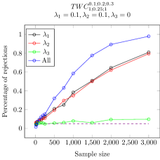
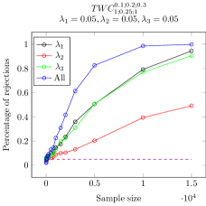
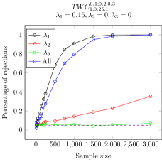
Figure 1: Results of Monte Carlo estimates of percentage of rejection of different null hypotheses of specified center symmetry, with increasing sample size and $f_{0}$ being the TWC with parameters $\rho_{12}=\rho_{23}=1,\rho_{13}=0.25$ and wrapped Cauchy marginal distributions with parameters $\beta_{1}=0.1,\beta_{2}=0.2,\beta_{3}=0.3$. The black line corresponds to the test $\mathcal{H}^{(n)}_{0;\mu;1}:\lambda_{1}=0\text{ vs }\mathcal{H}^{(n)}_{1;\mu;1}:\lambda_{1}\neq 0$, the red and green lines correspond to the analogous tests for $\lambda_{2}$ and $\lambda_{3}$ and the blue line corresponds to the test $\mathcal{H}^{(n)}_{0;\mu}:\boldsymbol{\lambda}=0\text{ vs }\mathcal{H}^{(n)}_{1;\mu}:\boldsymbol{\lambda}\neq 0$. The purple dotted line indicates 0.05.

After these extensive and general observations, we now investigate certain settings in more detail. To this end, Figure 1 shows plots of the Monte Carlo estimates of the probability of rejection of three different null hypotheses under specified symmetry center as the sample size increases. The blue line represents the power of the test for testing $\mathcal{H}^{(n)}_{0;\mu}:\boldsymbol{\lambda}=\boldsymbol{0}$, while the black, red and green lines represent the power of the test for testing for symmetry on each of the directions separately, meaning $\mathcal{H}^{(n)}_{0;\mu;i}:\lambda_{i}=0$ for $i=1,2,3$. The data are generated from the TWC, with parameters $\rho_{12}=\rho_{23}=1,\rho_{13}=0.25$ and wrapped Cauchy marginal distributions with parameters $\beta_{1}=0.1,\beta_{2}=0.2,\beta_{3}=0.3$. The three components are not independent, which explains why in the left plot there is some power of the test corresponding to $\lambda_{3}$, even though $\lambda_{3}=0$. In the first two plots, it is clear that the power of the test when testing all three components at the same time is higher than the power of the other tests. In the last plot, $\lambda_{1}$ is the only non-zero skewness parameter and thus the power of the test only for $\lambda_{1}$ is the most powerful. However, the power of the test for all three components is only slightly less powerful. These plots provide evidence in favor of using a test for symmetry on all the dimensions of the data at hand, instead of testing for symmetry for each component separately.

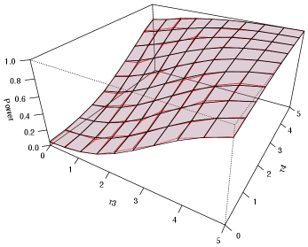
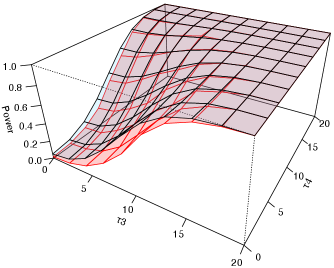
(a)	(b)
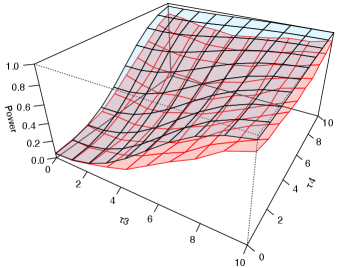
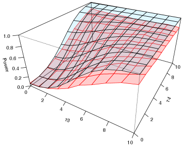
(c)	(d)

Figure 2: Plots of the theoretical (light blue) and simulated (red) power of the test for (a) $\phi^{\ast(n);\mu}$ with $f_{0}=BWC_{0.1,0.5,0.4}$, (b) $\phi^{\ast(n)}_{f_{0}}$ with $f_{0}=g_{0}=BWC_{0.9,0.9,0.4}$, (c) $\phi^{\ast(n)}_{f_{0}}$ with $f_{0}=BWC_{0.8,0.8,0.6}$, $g_{0}=BWC_{0.3,0.3,0.4}$ and (d) $\phi^{\ast(n)}_{f_{0}}$ with $f_{0}=S_{0.2,0.2,0.4}$, $g_{0}=S_{0.1,0.1,0.1}$.

Figure 2 is a plot of the theoretical power of the test, as given in Theorems 1 and 3, in light blue color, and the simulated power, as obtained by Monte Carlo simulations, in red color. For these plots we consider only $d=2$ and denote $\boldsymbol{\tau}_{\lambda}=(\tau_{3},\tau_{4})^{\prime}$. For the simulations, 1.000 repetitions were used for each value of $\boldsymbol{\lambda}=\boldsymbol{\tau}/\sqrt{n}$, and the sample size for each replication was $n=10.000$. In Figure 2(a), the results for the test for the specified symmetry center are plotted, with data being generated from the BWC distribution with parameters $\xi_{1}=0.1,\xi_{2}=0.5$ and $\tilde{\rho}=0.4$. We observe that the theoretical and estimated powers are almost identical. In Figures 2(b)-(d), the test for unspecified symmetry center is considered. In (b), the true and assumed densities $f_{0}$ and $g_{0}$ are chosen to be the same while, for (c) and (d), they are different. For (b), the distribution is chosen as the BWC with parameters $\xi_{1}=0.9,\xi_{2}=0.9$ and $\tilde{\rho}=0.4$. For small values of the skewness parameter the simulated power is lower than the theoretical one, as expected. For (c), the data are generated from the BWC with $\xi_{1}=0.3,\xi_{2}=0.3$ and $\rho=0.4$ while the test is built using the same distribution with $\xi_{1}=0.8,\xi_{2}=0.8$ and $\tilde{\rho}=0.6$. Finally, for (d), the data are generated from the Sine model with $\kappa_{1}=0.1,\kappa_{2}=0.1$ and $\rho=0.1$ and the test is built using the Sine model with $\kappa_{1}=0.2,\kappa_{2}=0.2$ and $\rho=0.4$. The simulated powers of the test in (c) and (d) are also lower than the theoretical ones. This can be improved by considering a larger $n$, which we did not attempt due to the computational complexity of the simulations. It is important to note that the high computational complexity refers to the resources needed to generate data from the underlying distributions, and not to the calculation of the test statistic, which can always be evaluated within seconds. We note that the difference between theoretical and practical power is the smallest when $f_{0}=g_{0}$.

Table 1: Percentage of rejections for $\phi^{\ast(n);\mu}$ when $d=2$. The data are generated using the model mentioned, $n$ represents the sample size and $\boldsymbol{\lambda}$ the value of the skewness parameter.

	$\boldsymbol{\lambda}$	$(0,0)$	$(0.1,0)$	$(0.1,0.1)$	$(0.2,0.1)$	$(0.2,0.2)$
Model	$n$
	200	0.058	0.118	0.225	0.488	0.717
$I_{0.1;0.1}$	500	0.056	0.253	0.501	0.893	0.985
	1000	0.042	0.492	0.804	1.000	1.000
	200	0.051	0.114	0.202	0.448	0.720
$S_{1;1;0.1}$	500	0.043	0.280	0.472	0.886	0.977
	1000	0.045	0.484	0.808	0.993	1.000
	200	0.047	0.118	0.194	0.456	0.710
$C_{1;1;0.1}$	500	0.046	0.269	0.459	0.870	0.975
	1000	0.047	0.456	0.808	0.996	1.000
	200	0.048	0.121	0.242	0.569	0.780
$BWC_{0.1;0.5;0.3}$	500	0.045	0.292	0.551	0.923	0.992
	1000	0.047	0.494	0.857	1.000	1.000
	200	0.044	0.144	0.224	0.512	0.730
$MNNTS_{2}$	500	0.051	0.268	0.521	0.895	0.984
	1000	0.048	0.502	0.829	0.996	1.000

Table 2: Percentage of rejections for $\phi^{\ast(n);\mu}$ when $d=3$. The data are generated using the model mentioned, $n$ represents the sample size and $\boldsymbol{\lambda}$ the value of the skewness parameter.

	$\boldsymbol{\lambda}$	$(0,0,0)$	$(0.1,0,0)$	$(0.2,0.1,0)$	$(0.2,0.2,0.2)$
Model	$n$
	200	0.041	0.109	0.414	0.821
$I_{0.1;0.1;0.1}$	500	0.054	0.238	0.854	0.999
	1000	0.063	0.451	0.994	1.000
	200	0.066	0.116	0.440	0.834
$TWC_{5;2;0.1}^{0.1;0.1;0.1}$	500	0.048	0.229	0.852	0.998
	1000	0.047	0.448	0.992	1.000
	200	0.070	0.116	0.440	0.861
$MNNTS_{3}$	500	0.046	0.220	0.864	1.000
	1000	0.061	0.446	0.995	1.000

Table 3: Percentage of rejections for $\phi^{\ast(n);\mu}$ when $d=5,10,20$. The data are generated using the model mentioned, $n$ represents the sample size and $\boldsymbol{\lambda}$ the value of the skewness parameter. Note that the missing entries correspond to non-allowed settings where the sum of the components of $\boldsymbol{\lambda}$ would exceed 1.

		$\boldsymbol{\lambda}$	$(0,\ldots,0)$	$(0.05,\ldots,0.05)$	$(0.1,\ldots,0.1)$	$(0.15,\ldots,0.15)$
Model	$d$	$n$
		200	0.041	0.134	0.350	0.705
$I_{0.1;\ldots;0.1}$	$5$	500	0.049	0.206	0.773	0.998
		1000	0.049	0.442	0.979	1.000
		200	0.047	0.080	0.212	0.516
$I_{0.6;\ldots;0.6}$	$5$	500	0.051	0.131	0.534	0.925
		1000	0.040	0.278	0.884	0.997
		200	0.049	0.118	0.346	0.709
$MNNTS_{5}$	5	500	0.050	0.222	0.780	0.992
		1000	0.066	0.447	0.982	1.000
		200	0.051	0.147	0.484	-
$I_{0.1;\ldots;0.1}$	10	500	0.047	0.321	0.937	-
		1000	0.052	0.640	1.000	-
		200	0.040	0.089	0.316	-
$I_{0.6;\ldots;0.6}$	10	500	0.044	0.197	0.773	-
		1000	0.050	0.440	0.991	-
		200	0.049	0.162	-	-
$I_{0.1;\ldots;0.1}$	20	500	0.047	0.515	-	-
		1000	0.055	0.866	-	-
		1500	0.041	0.983	-	-
		200	0.043	0.088	-	-
$I_{0.6;\ldots;0.6}$	20	500	0.046	0.284	-	-
		1000	0.055	0.623	-	-
		1500	0.050	0.859	-	-

Table 4: Percentage of rejections for $\phi^{\ast(n)}_{f_{0}}$ when $d=2$. The data are generated using the model $g_{0}$ and the test statistic is evaluated using the model $f_{0}$, $n$ represents the sample size and $\boldsymbol{\lambda}$ the value of the skewness parameter.

$g_{0}=S_{1;1;0.7}$
	$\boldsymbol{\lambda}$	$(0,0)$	$(0.1,0)$	$(0.1,0.1)$	$(0.2,0.1)$	$(0.2,0.2)$
$f_{0}$	$n$
	500	0.058	0.069	0.147	0.290	0.387
$S_{0.5;0.5;0.1}$	1000	0.050	0.108	0.255	0.494	0.673
	5000	0.059	0.402	0.865	0.996	1.000
	$\boldsymbol{\lambda}$	$(0,0)$	$(0.2,0)$	$(0.4,0)$	$(0.6,0)$	$(0.8,0)$
	500	0.067	0.068	0.055	0.099	0.409
$I_{0.1;0.1}$	1000	0.045	0.061	0.069	0.139	0.690
	5000	0.062	0.115	0.097	0.522	1.000
	500	0.049	0.043	0.061	0.123	0.254
$BWC_{0.5;0.5;0.3}$	1000	0.048	0.069	0.118	0.217	0.454
	5000	0.054	0.127	0.371	0.823	0.998

Table 5: Percentage of rejections for $\phi^{\ast(n)}_{f_{0}}$ when $d=3$. The data are generated using the model $g_{0}$ and the test statistic is evaluated using the model $f_{0}$, $n$ represents the sample size and $\boldsymbol{\lambda}$ the value of the skewness parameter.

$g_{0}=MNNTS_{3}$
	$\boldsymbol{\lambda}$	$(0,0,0)$	$(0.1,0,0)$	$(0.2,0.1,0)$	$(0.2,0.2,0.2)$
$f_{0}$	$n$
	200	0.078	0.095	0.142	0.210
$I_{0.1;0.1;0.1}$	500	0.052	0.089	0.202	0.397
	1000	0.058	0.109	0.324	0.646
	200	0.056	0.077	0.213	0.644
$TWC_{1;1.2;0.5}^{0.1;0.2;0.3}$	500	0.054	0.097	0.265	0.967
	1000	0.059	0.088	0.446	1.000

Table 6: Percentage of rejections for $\phi^{\ast(n)}_{f_{0}}$ when $d=3$. The data are generated using the model $g_{0}$ and the test statistic is evaluated using the model $f_{0}$, $n$ represents the sample size and $\boldsymbol{\lambda}$ the value of the skewness parameter.

$g_{0}=TWC_{5;2;0.1}^{0.1;0.1;0.1}$
	$\boldsymbol{\lambda}$	$(0,0,0)$	$(0.1,0,0)$	$(0.1,0.1,0)$	$(0.1,0.1,0.1)$
$f_{0}$	$n$
	500	0.042	0.232	0.440	0.596
$I_{0.1;0.1;0.1}$	1000	0.052	0.436	0.742	0.906
	5000	0.056	0.982	1.000	1.000
	500	0.062	0.226	0.405	0.530
$I_{0.1;0.2;0.3}$	1000	0.064	0.424	0.720	0.860
	5000	0.061	0.990	1.000	1.000
	500	0.035	0.201	0.384	0.585
$TWC_{5;2;0.1}^{0.1;0.1;0.1}$	1000	0.052	0.389	0.746	0.896
	5000	0.047	0.984	1.000	1.000
	500	0.044	0.171	0.248	0.499
$TWC_{1;1.2;0.5}^{0.1;0.2;0.3}$	1000	0.051	0.228	0.429	0.785
	5000	0.040	0.461	0.899	1.000

6 Application: protein data

In this section, our new tests are applied to a real-world dataset. The chosen dataset includes data from the protein folding problem, which involves predicting the three-dimensional structure of a protein using the sequence of amino acids that make up the protein. This is an important and challenging problem with implications to vaccine and medicine development. Deep learning models like AlphaFold, whose lead scientists won the Nobel Prize in Chemistry in 2024, have drastically improved accuracy, solving protein structures that were unknown for decades. However, the problem is not yet completely solved. The open questions include dynamics, mutants, accuracy (lopez-sagaseta_severe_2025 ; chakravarty_alphafold_2024 ). A natural extension of protein folding is RNA folding, for which even the most advanced protein prediction algorithms fall short (kwon_rna_2025 ).

Many papers in the literature model datasets relating to the protein folding problem using distributions on the torus, see for example kato2024versatiletrivariatewrappedcauchy ; mardia_multivariate_2008 ; mardia_mixtures_2012 . Mardia13 reviews statistical advances in some major active areas of protein structural bioinformatics, including structure prediction. Most efforts have employed symmetric distributions. Based on visual inspection of such datasets, biologists believe that asymmetric distributions should be used (Mardia13 ). Our aim here is to provide a statistical confirmation of this fact.

Proteins are made up of amino acids, which in turn are made up of the backbone and the sidechains. In this analysis, we only focus on the backbone but one could also consider the angles formed in the sidechains. The backbone consists of two flexible chemical bonds, NH-C$\alpha$ and C$\alpha$-CO, where C$\alpha$ denotes the central Carbon atom. The angle that can be found at the beginning of each residue is the NH-C$\alpha$ torsion angle, denoted by $\phi$ and at the end is the C$\alpha$-CO torsion angle, denoted by $\psi$. The peptide bond, CO-NH, is a torsion angle that cannot rotate freely, due to the physiochemical properties and is denoted by $\omega$. These angles need to be studied as specific combinations of them allow the favourable hydrogen bonding patterns, while others can ‘result in clashes within the backbone or between adjacent sidechains’ (jacobsen_introduction_2023 ).

For the present data analysis, we consider position 55 at 2000 randomly selected times in the molecular dynamic trajectory of the SARS-CoV-2 spike domain from genna_sars-cov-2_2020 . The position occurs in $\alpha$-helix throughout the trajectory. DPPS kabsch_dictionary_1983 is used to compute the secondary structure and cock_biopython_2009 to verify the chains. Since we only use data from an $\alpha$-helix, the data used have a unique mode, which can also be observed by the plot of the angles in Figure 3. It is a known fact in biology (see tooze_introduction_1998 ) that the $\alpha$-helix occurs when the consecutive ($\phi$, $\psi$) angle pairs are around $(-1.05\text{ rads},-0.87\text{ rads})$ (or equivalently $(-60^{\circ},-50^{\circ})$), for the shape of the helix to come up. The angle $\omega$ can only take the values $0$ and $\pi$, but usually the values are recorded with noise. In the case of our data, from the plot of Figure 3, the theoretical value is $\omega=\pi$ rads. Thus the theoretical symmetry center for our specified-center test will be $(-1.05,-0.87,\pi)$. In Figure 3, the theoretical value of the mean is plotted in red and the estimated one in blue, for each angle.

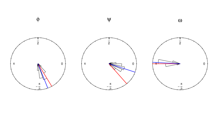
Figure 3: Rose plots of the protein data. The theoretical mean $(-1.05,-0.87,\pi)$ is plotted in red and the estimated one $(-1.21,-0.33,3.08)$ is plotted in blue.

As expected and confirming biologists’ observations, the test for specified symmetry center $Q_{f_{0}}^{\ast(n);\boldsymbol{\mu}}$ rejects the null hypothesis of symmetry $\mathcal{H}^{(n)}_{0;\mu}$ at all commonly used levels of significance. We next applied the test for unspecified symmetry center, $Q_{f_{0}}^{\ast(n)}$ with the TWCC as $f_{0}$, which also rejects the null hypothesis of symmetry $\mathcal{H}^{(n)}_{0}$ at all commonly used levels of significance. This supports the biologists’ belief that the data is not symmetric, and thus must be modeled using skewed distributions. The test can also be performed for only $(\phi,\psi)$, a dihedral pair which is commonly modeled in the literature (see for example mardia_mixtures_2012 ; kato_mobius_2015 ; singh_probabilistic_2002 ), and the conclusion remains the same.

7 Conclusion

In this paper we have proposed tests for symmetry for data on a hyper-torus, using the Le Cam approach for building optimal tests. Two different tests are proposed, depending on whether the symmetry center is specified or needs to be calculated. In both cases, the distribution of the test statistic under the null hypothesis of symmetry is the chi-squared distribution, with $d$ degrees of freedom. The asymptotic distribution under local alternatives is a non-central chi-square distribution with $d$ degrees of freedom, with different centrality parameter for the two tests. For both cases, we also provide, using Stein’s Method, bounds on the distributional distance between the distribution of the test statistic and its limiting distribution.

The finite sample performance of the proposed tests is also investigated using simulation studies. Data from different distributions were generated, in different dimensions $d$, and, in the case of the test corresponding to the case of the unspecified median, different distributions were used to build the tests. Our tests’ power was also exhibited in a real world scenario, using data from the protein structure prediction problem.

The tests are built to test for symmetry in the sine-skewed family (1). It can be proven that the tests are also optimal for testing for symmetry in the following skewed family, with alternative skewing transformation:

$$\boldsymbol{\theta}\mapsto f_{\boldsymbol{\mu},\boldsymbol{\lambda}}(\boldsymbol{\theta};\boldsymbol{\vartheta}):=f_{0}(\boldsymbol{\theta}-\boldsymbol{\mu};\boldsymbol{\vartheta})\prod_{j=1}^{d}\left(1+\lambda_{j}\sin(\theta_{j}-\mu_{j})\right)\quad\mbox{subject to}\,\,|\lambda_{j}|\leq 1,j=1,\ldots,d$$ (41)

since the central sequence and the Fisher Information matrix will be the same as the model under consideration in this paper. This implies that the ULAN property will also be the same and so all results mentioned in this paper hold for (41) as well.

Acknowledgments: The authors would like to thank Thomas Hamelryck and Ola Rønning for the protein data and Ivan Nourdin for constructive conversations.

Funding: The third author was funded by the Luxembourg National Research Fund (FNR), grant reference PRIDE/21/16747448/MATHCODA.

S1 Proofs

S1.1 Proof of Proposition 1

Before the proof, we state for the sake of readability the definition of quadratic mean differentiable functions (see Definition 12.2.1 from [4]), which is needed to prove the proposition.

Definition 1.

The model $\left(P_{\theta}:\theta\in\Theta\right)$ is said to be differentiable in quadratic mean if at an inner point $\theta_{0}\in\Theta$ there exists a measurable function $\dot{\ell}_{\theta_{0}}:\mathcal{X}\rightarrow\mathbb{R}^{k}$ such that

$$\int_{\mathcal{X}}\left\{\sqrt{p_{\theta_{0}+h}}-\sqrt{p_{\theta_{0}}}-\frac{1}{2}h^{\prime}\dot{\ell}_{\theta_{0}}\sqrt{p_{\theta_{0}}}\right\}^{2}{\mathrm{d}}\mu=o\left(||h||^{2}\right)\quad\text{as }||h||\rightarrow 0,$$ (S42)

where $p_{\theta}$ is the density of $P_{\theta}$ with respect to some measure $\mu$ and $\frac{1}{2}\dot{\ell}_{\theta_{0}}\sqrt{p_{\theta_{0}}}$ is the quadratic mean derivative at $\theta_{0}$.

Proof of Proposition 1.

“$\Leftarrow$" is immediate by taking $\boldsymbol{h}=(h_{1}^{1},\ldots,h_{1}^{k},0,\ldots,0)^{\prime}$ in (S42).

“$\Rightarrow$" Assume that $\boldsymbol{\mu}\mapsto f(\boldsymbol{x};\boldsymbol{\mu})$ is QMD. Using (S42) and defining

$$A:=\int_{\mathcal{X}}\Biggl(f^{1/2}(\boldsymbol{x};\boldsymbol{\mu}_{0}+\boldsymbol{h}_{1}) g^{1/2}(\boldsymbol{x};\boldsymbol{\mu}_{0}+\boldsymbol{h}_{1},\boldsymbol{h}_{2})-f^{1/2}(\boldsymbol{x};\boldsymbol{\mu}_{0})$$

$$- \boldsymbol{h}^{\prime}\left.\begin{pmatrix}\nabla_{\boldsymbol{\mu}}f^{1/2}(\boldsymbol{x};\boldsymbol{\mu})\\ f^{1/2}(\boldsymbol{x};\boldsymbol{\mu})\nabla_{\boldsymbol{\lambda}}g^{1/2}(\boldsymbol{x};\boldsymbol{\mu},\boldsymbol{\lambda})\end{pmatrix}\right|_{\begin{subarray}{c}\scriptscriptstyle{\boldsymbol{\mu}=\boldsymbol{\mu}_{0}}\\ \scriptscriptstyle{\boldsymbol{\lambda}=0}\end{subarray}}\Biggr)^{2}{\mathrm{d}}\boldsymbol{x}$$

for $\boldsymbol{h}=(\boldsymbol{h}_{1}^{\prime},\boldsymbol{h}_{2}^{\prime})^{\prime}$, $\boldsymbol{h}_{1}\in\mathbb{R}^{k}$ and $\boldsymbol{h}_{2}\in\mathbb{R}^{m}$, we need to prove that $A=o(||\boldsymbol{h}||^{2})$. Condition (iii) of the statement of the proposition ensures that the partial derivatives of the square roots of the functions are well defined. We can bound $A$ by $3(A_{1}+A_{2}+A_{3})$, where

$$A_{1}: =\int_{\mathcal{X}}\Biggl(f^{1/2}(\boldsymbol{x};\boldsymbol{\mu}_{0}+\boldsymbol{h}_{1})-f^{1/2}(\boldsymbol{x};\boldsymbol{\mu}_{0})-\boldsymbol{h}_{1}^{\prime}\left.\nabla_{\boldsymbol{\mu}}f^{1/2}(\boldsymbol{x};\boldsymbol{\mu})\right|_{{\scriptscriptstyle{\boldsymbol{\mu}=\boldsymbol{\mu}_{0}}}}\Biggr)^{2}{\mathrm{d}}\boldsymbol{x},$$

$$A_{2}: =\int_{\mathcal{X}}\Biggl(f^{1/2}(\boldsymbol{x};\boldsymbol{\mu}_{0}+\boldsymbol{h}_{1})g^{1/2}(\boldsymbol{x};\boldsymbol{\mu}_{0}+\boldsymbol{h}_{1},\boldsymbol{h}_{2})-f^{1/2}(\boldsymbol{x};\boldsymbol{\mu}_{0}+\boldsymbol{h}_{1})$$

$$\hskip 85.35826pt-\boldsymbol{h}_{2}^{\prime}\left.f^{1/2}(\boldsymbol{x};\boldsymbol{\mu}_{0}+\boldsymbol{h}_{1})\nabla_{\boldsymbol{\lambda}}g^{1/2}(\boldsymbol{x};\boldsymbol{\mu},\boldsymbol{\lambda})\right|_{\begin{subarray}{c}\scriptscriptstyle{\boldsymbol{\mu}=\boldsymbol{\mu}_{0}+\boldsymbol{h}_{1}}\\ \scriptscriptstyle{\boldsymbol{\lambda}=0}\end{subarray}}\Biggr)^{2}{\mathrm{d}}\boldsymbol{x},$$

$$A_{3}: =\int_{\mathcal{X}}\Biggl(\boldsymbol{h}_{2}^{\prime}\biggl(\left.f^{1/2}(\boldsymbol{x};\boldsymbol{\mu}_{0}+\boldsymbol{h}_{1})\nabla_{\boldsymbol{\lambda}}g^{1/2}(\boldsymbol{x};\boldsymbol{\mu},\boldsymbol{\lambda})\right|_{\begin{subarray}{c}\scriptscriptstyle{\boldsymbol{\mu}=\boldsymbol{\mu}_{0}+\boldsymbol{h}_{1}}\\ \scriptscriptstyle{\boldsymbol{\lambda}=0}\end{subarray}}$$

$$\hskip 85.35826pt-f^{1/2}(\boldsymbol{x};\boldsymbol{\mu}_{0})\left.\nabla_{\boldsymbol{\lambda}}g^{1/2}(\boldsymbol{x};\boldsymbol{\mu},\boldsymbol{\lambda})\right|_{\begin{subarray}{c}\scriptscriptstyle{\boldsymbol{\mu}=\boldsymbol{\mu}_{0}}\\ \scriptscriptstyle{\boldsymbol{\lambda}=0}\end{subarray}}\biggr)\Biggr)^{2}{\mathrm{d}}\boldsymbol{x}.$$

Showing that $A_{1}=o(\parallel\boldsymbol{h}_{1}\parallel^{2})$ and $A_{2}=o(\parallel\boldsymbol{h}_{2}\parallel^{2})=A_{3}$ implies that $A=o(||\boldsymbol{h}||^{2})$. Note that conditions (v) and (vi) in the statement of the proposition are needed for $A_{1}$, $A_{2}$ and $A_{3}$ to be finite. The result concerning $A_{1}$ follows immediately from Definition 1 and the fact that $\boldsymbol{\mu}\mapsto f(\boldsymbol{x};\boldsymbol{\mu})$ is QMD. For the part involving $A_{2}$, we rewrite it as

$$A_{2}=\int_{\mathcal{X}}f(\boldsymbol{x};\boldsymbol{\mu}_{0}+\boldsymbol{h}_{1})\Biggl(g^{1/2}(\boldsymbol{x};\boldsymbol{\mu}_{0}+\boldsymbol{h}_{1},\boldsymbol{h}_{2})-1-\boldsymbol{h}_{2}^{\prime}\left.\nabla_{\boldsymbol{\lambda}}g^{1/2}(\boldsymbol{x};\boldsymbol{\mu},\boldsymbol{\lambda})\right|_{\begin{subarray}{c}\scriptscriptstyle{\boldsymbol{\mu}=\boldsymbol{\mu}_{0}+\boldsymbol{h}_{1}}\\ \scriptscriptstyle{\boldsymbol{\lambda}=0}\end{subarray}}\Biggr)^{2}{\mathrm{d}}\boldsymbol{x}.$$

From assumption (i), $g$ is a.e. $\mathcal{C}^{1}$ in $\boldsymbol{\lambda}$, hence by the Mean Value Theorem it holds that

$$\boldsymbol{h}_{2}^{\prime}\nabla_{\boldsymbol{\lambda}}\left.g^{1/2}(\boldsymbol{x};\boldsymbol{\mu},\boldsymbol{\lambda})\right| {}_{\begin{subarray}{c}\scriptscriptstyle{\boldsymbol{\mu}=\boldsymbol{\mu}_{0}+\boldsymbol{h}_{1}}\\ \scriptscriptstyle{\boldsymbol{\lambda}=\boldsymbol{\lambda}^{\ast}_{\boldsymbol{h}_{2}}}\end{subarray}}$$

$$=g^{1/2} (\boldsymbol{x};\boldsymbol{\mu}_{0}+\boldsymbol{h}_{1},\boldsymbol{h}_{2})-g^{1/2}(\boldsymbol{x};\boldsymbol{\mu}_{0}+\boldsymbol{h}_{1},\boldsymbol{0})=g^{1/2}(\boldsymbol{x};\boldsymbol{\mu}_{0}+\boldsymbol{h}_{1},\boldsymbol{h}_{2})-1$$

for some $\boldsymbol{\lambda}^{\ast}_{\boldsymbol{h}_{2}}$ which lies on the line connecting $\boldsymbol{0}$ and $\boldsymbol{h}_{2}$, where the last equality follows from assumption (iv). This entails that

$$A_{2} =\int_{\mathcal{X}}f(\boldsymbol{x};\boldsymbol{\mu}_{0}+\boldsymbol{h}_{1})\Biggl(\boldsymbol{h}_{2}^{\prime}\left(\nabla_{\boldsymbol{\lambda}}\left.g^{1/2}(\boldsymbol{x};\boldsymbol{\mu},\boldsymbol{\lambda})\right|_{\begin{subarray}{c}\scriptscriptstyle{\boldsymbol{\mu}=\boldsymbol{\mu}_{0}+\boldsymbol{h}_{1}}\\ \scriptscriptstyle{\boldsymbol{\lambda}=\boldsymbol{\lambda}^{\ast}_{\boldsymbol{h}_{2}}}\end{subarray}}-\left.\nabla_{\boldsymbol{\lambda}}g^{1/2}(\boldsymbol{x};\boldsymbol{\mu},\boldsymbol{\lambda})\right|_{\begin{subarray}{c}\scriptscriptstyle{\boldsymbol{\mu}=\boldsymbol{\mu}_{0}+\boldsymbol{h}_{1}}\\ \scriptscriptstyle{\boldsymbol{\lambda}=0}\end{subarray}}\right)\Biggr)^{2}{\mathrm{d}}\boldsymbol{x}$$

$$\leq||\boldsymbol{h}_{2}||^{2}\int_{\mathcal{X}}f(\boldsymbol{x};\boldsymbol{\mu}_{0}+\boldsymbol{h}_{1})\Biggl|\Biggl|\nabla_{\boldsymbol{\lambda}}\left.g^{1/2}(\boldsymbol{x};\boldsymbol{\mu},\boldsymbol{\lambda})\right|_{\begin{subarray}{c}\scriptscriptstyle{\boldsymbol{\mu}=\boldsymbol{\mu}_{0}+\boldsymbol{h}_{1}}\\ \scriptscriptstyle{\boldsymbol{\lambda}=\boldsymbol{\lambda}^{\ast}_{\boldsymbol{h}_{2}}}\end{subarray}}-\left.\nabla_{\boldsymbol{\lambda}}g^{1/2}(\boldsymbol{x};\boldsymbol{\mu},\boldsymbol{\lambda})\right|_{\begin{subarray}{c}\scriptscriptstyle{\boldsymbol{\mu}=\boldsymbol{\mu}_{0}+\boldsymbol{h}_{1}}\\ \scriptscriptstyle{\boldsymbol{\lambda}=0}\end{subarray}}\Biggr|\Biggr|^{2}{\mathrm{d}}\boldsymbol{x},$$

where the last inequality follows by Cauchy-Schwarz. The triangle inequality combined with assumption (ii) yields

$$\Biggl|\Biggl|\nabla_{\boldsymbol{\lambda}}\left.g^{1/2}(\boldsymbol{x};\boldsymbol{\mu},\boldsymbol{\lambda})\right|_{\begin{subarray}{c}\scriptscriptstyle{\boldsymbol{\mu}=\boldsymbol{\mu}_{0}+\boldsymbol{h}_{1}}\\ \scriptscriptstyle{\boldsymbol{\lambda}=\boldsymbol{\lambda}^{\ast}_{\boldsymbol{h}_{2}}}\end{subarray}}-\left.\nabla_{\boldsymbol{\lambda}}g^{1/2}(\boldsymbol{x};\boldsymbol{\mu},\boldsymbol{\lambda})\right|_{\begin{subarray}{c}\scriptscriptstyle{\boldsymbol{\mu}=\boldsymbol{\mu}_{0}+\boldsymbol{h}_{1}}\\ \scriptscriptstyle{\boldsymbol{\lambda}=0}\end{subarray}}\Biggr|\Biggr|\leq 2C\ell(\boldsymbol{x};\boldsymbol{\mu}_{0}+\boldsymbol{h}_{1})$$

for $C\in\mathbb{R}^{+}$ independent of $\lambda^{\ast}_{\boldsymbol{h}_{2}}$ and hence of $\boldsymbol{h}_{2}$. The Dominated Convergence Theorem allows us to conclude that $A_{2}=o(\parallel\boldsymbol{h}_{2}\parallel^{2})$.

Finally for $A_{3}$, we also have by the triangle inequality and assumption (ii) that

$$\Biggl|\Biggl|\left.f^{1/2}(\boldsymbol{x};\boldsymbol{\mu}_{0}+\boldsymbol{h}_{1})\nabla_{\boldsymbol{\lambda}}g^{1/2}(\boldsymbol{x};\boldsymbol{\mu},\boldsymbol{\lambda})\right|_{\begin{subarray}{c}\scriptscriptstyle{\boldsymbol{\mu}=\boldsymbol{\mu}_{0}+\boldsymbol{h}_{1}}\\ \scriptscriptstyle{\boldsymbol{\lambda}=0}\end{subarray}}-f^{1/2}(\boldsymbol{x};\boldsymbol{\mu}_{0})\left.\nabla_{\boldsymbol{\lambda}}g^{1/2}(\boldsymbol{x};\boldsymbol{\mu},\boldsymbol{\lambda})\right|_{\begin{subarray}{c}\scriptscriptstyle{\boldsymbol{\mu}=\boldsymbol{\mu}_{0}}\\ \scriptscriptstyle{\boldsymbol{\lambda}=0}\end{subarray}}\Biggr|\Biggr|$$

$$\leq f^{1/2}(\boldsymbol{x};\boldsymbol{\mu}_{0}+\boldsymbol{h}_{1})\Biggl|\Biggl|\left.\nabla_{\boldsymbol{\lambda}}g^{1/2}(\boldsymbol{x};\boldsymbol{\mu},\boldsymbol{\lambda})\right|_{\begin{subarray}{c}\scriptscriptstyle{\boldsymbol{\mu}=\boldsymbol{\mu}_{0}+\boldsymbol{h}_{1}}\\ \scriptscriptstyle{\boldsymbol{\lambda}=0}\end{subarray}}\Biggr|\Biggr|+f^{1/2}(\boldsymbol{x};\boldsymbol{\mu}_{0})\Biggl|\Biggl|\left.\nabla_{\boldsymbol{\lambda}}g^{1/2}(\boldsymbol{x};\boldsymbol{\mu},\boldsymbol{\lambda})\right|_{\begin{subarray}{c}\scriptscriptstyle{\boldsymbol{\mu}=\boldsymbol{\mu}_{0}}\\ \scriptscriptstyle{\boldsymbol{\lambda}=0}\end{subarray}}\Biggr|\Biggr|$$

$$\leq C\left(f^{1/2}(\boldsymbol{x};\boldsymbol{\mu}_{0}+\boldsymbol{h}_{1})\ell(\boldsymbol{x};\boldsymbol{\mu}_{0}+\boldsymbol{h}_{1})+f^{1/2}(\boldsymbol{x};\boldsymbol{\mu}_{0})\ell(\boldsymbol{x};\boldsymbol{\mu}_{0})\right)$$

which is an integrable function not depending on $\boldsymbol{h}_{2}$. The Dominated Convergence Theorem thus applies and gives $A_{3}=o(\parallel\boldsymbol{h}_{2}\parallel^{2})$. ∎

S1.2 Proof of Proposition 2

For the sake of a better understanding, we recall here Lemma 2.3 of [1], on which the proof is based.

Lemma S3.

Denote by $P^{(n)}_{1}$ and $P^{(n)}_{0}$ two sequences of probability measures on measurable spaces $\left(\mathcal{X}^{(n)},\mathcal{A}^{(n)}\right)$. For all $n$, let $\mathcal{A}_{t}^{(n)}\subset\mathcal{A}_{t+1}^{(n)}$ be a filtration such that $\mathcal{A}_{n}^{(n)}=\mathcal{A}^{(n)}$, and denote by $P^{(n)}_{1,t}$ and $P^{(n)}_{0,t}$ the restrictions to $\mathcal{A}_{t}^{(n)}$ of $P^{(n)}_{1}$ and $P^{(n)}_{0}$, respectively. Assuming that $P^{(n)}_{1,t}$ is absolutely continuous (on $\mathcal{A}_{t}^{(n)}$) with respect to $P^{(n)}_{0,t}$, let $\alpha_{0}^{(n)}=1,\alpha_{t}^{(n)}=dP^{(n)}_{1,t}/dP^{(n)}_{0,t}$ and $\xi_{t}^{(n)}=\left(\alpha_{t}^{(n)}/\alpha_{t-1}^{(n)}\right)^{1/2}-1$. Assume that the random variables $\zeta_{t}^{(n)}$ satisfy the following conditions (all convergences are in $P^{(n)}_{0}$-probability, as $n\rightarrow\infty$; expectations are also taken with respect to $P^{(n)}_{0}$):

1. $\mathbb{E}\left[\sum_{t=1}^{n}\left(\zeta_{t}^{(n)}-\xi_{t}^{(n)}\right)^{2}\right]\rightarrow 0$;

2. $\sup_{n}\mathbb{E}\left[\sum_{t=1}^{n}\left(\zeta_{t}^{(n)}\right)^{2}\right]<\infty$;

3. $\max_{1\leq t\leq n}\left|\zeta_{t}^{(n)}\right|\rightarrow 0$;

4. $\sum_{t=1}^{n}\left(\zeta_{t}^{(n)}\right)^{2}-\frac{\left(\uptau^{(n)}\right)^{2}}{4}\rightarrow 0$ for some non-random sequence $\left(\uptau^{(n)},n\in\mathbb{N}\right)$ such that $\sup_{n}\left(\uptau^{(n)}\right)^{2}<\infty$;

5. $\sum_{t=1}^{n}\mathbb{E}\left\{\left(\zeta_{t}^{(n)}\right)^{2}I\left[\left|\zeta_{t}^{(n)}\right|>\frac{1}{2}\right]\Bigg|\mathcal{A}^{(n)}_{t-1}\right\}\rightarrow 0$;

6. $\mathbb{E}\left[\zeta_{t}^{(n)}|\mathcal{A}^{(n)}_{t-1}\right]=0$;

7. $\sum_{t=1}^{n}\mathbb{E}\left[\left(\xi_{t}^{(n)}\right)^{2}+2\xi_{t}^{(n)}|\mathcal{A}^{(n)}_{t-1}\right]\rightarrow 0$.

Then, under $P_{0}^{(n)}$, as $n\rightarrow\infty$,

$$\Lambda^{(n)}=\log\left(dP_{1}^{(n)}/P_{0}^{(n)}\right)=2\sum_{t=1}^{n}\zeta_{t}^{(n)}-\left(\uptau^{(n)}\right)^{2}/2+o_{P}(1),$$

and the distribution of $\left[\Lambda^{(n)}+\left(\uptau^{(n)}\right)^{2}/2\right]/\uptau^{(n)}$ is asymptotically standard normal.

Before proceeding to the proof of Proposition 2, we match the notation from this lemma with that in our paper:

$$\alpha_{t}^{(n)}=\frac{dP^{(n)}_{1,t}}{dP^{(n)}_{0,t}}=\prod_{i=1}^{t}\frac{f_{\boldsymbol{\mu}^{(n)}+n^{-1/2}\boldsymbol{\tau}^{(n)}_{\mu},n^{-1/2}\boldsymbol{\tau}^{(n)}_{\lambda}}(\boldsymbol{\theta}_{i})}{f_{\boldsymbol{\mu}^{(n)},\boldsymbol{0}}(\boldsymbol{\theta}_{i})}$$

$$\xi_{t}^{(n)}=\left(\frac{f_{\boldsymbol{\mu}^{(n)}+n^{-1/2}\boldsymbol{\tau}^{(n)}_{\mu},n^{-1/2}\boldsymbol{\tau}^{(n)}_{\lambda}}(\boldsymbol{\theta}_{t})}{f_{\boldsymbol{\mu}^{(n)},\boldsymbol{0}}(\boldsymbol{\theta}_{t})}\right)^{1/2}-1,$$

$$\zeta_{t}^{(n)}=\frac{1}{2\sqrt{n}}\boldsymbol{\tau}^{(n)\prime}\Delta_{f_{0};t}^{(n)}(\boldsymbol{\mu}^{(n)})=\frac{1}{2\sqrt{n}}\Biggl(\sum_{j=1}^{d}\tau_{j}^{(n)}\phi^{f_{0}}_{j}(\boldsymbol{\theta}_{t}-\boldsymbol{\mu}^{(n)})+\sum_{j=d+1}^{2d}\tau_{j}^{(n)}\sin(\theta_{tj}-\mu_{j}^{(n)})\Biggr),$$

$$\left(\uptau^{(n)}\right)^{2}=\boldsymbol{\tau}^{(n)\prime}\Gamma_{f_{0}}\boldsymbol{\tau}^{(n)}.$$

Note that $\sup_{n}\left(\uptau^{(n)}\right)<\infty$, so the assumption in (iv) is satisfied. Now we can prove Proposition 2.

Proof of Proposition 2.

Proving that Lemma S3 holds in our setting for family $P^{(n)}_{f_{0}}$ implies that Proposition 2 holds. Thus, we need to check that the conditions of Lemma S3 hold.

(i) Straightforward calculations yield

$$\mathbb{E} \left[\sum_{t=1}^{n}\left(\zeta_{t}^{(n)}-\xi_{t}^{(n)}\right)^{2}\right]=n\ \mathbb{E}\left[\left(\frac{\boldsymbol{\tau}^{(n)\prime}}{2\sqrt{n}}\Delta_{f_{0}}^{(n)}(\boldsymbol{\mu}^{(n)})-\frac{f^{1/2}_{\boldsymbol{\mu}^{(n)}+n^{-1/2}\boldsymbol{\tau}^{(n)}_{\mu},n^{-1/2}\boldsymbol{\tau}^{(n)}_{\lambda}}(\boldsymbol{\theta})}{f^{1/2}_{\boldsymbol{\mu}^{(n)},\boldsymbol{0}}(\boldsymbol{\theta})}+1\right)^{2}\right]$$

$$=n\int_{[-\pi,\pi)^{d}}\Biggl(\frac{\boldsymbol{\tau}^{(n)\prime}}{2\sqrt{n}}\nabla\log\left(f_{\boldsymbol{\mu}^{(n)},\boldsymbol{0}}(\boldsymbol{\theta})\right)-\frac{f^{1/2}_{\boldsymbol{\mu}^{(n)}+n^{-1/2}\boldsymbol{\tau}^{(n)}_{\mu},n^{-1/2}\boldsymbol{\tau}^{(n)}_{\lambda}}(\boldsymbol{\theta})}{f^{1/2}_{\boldsymbol{\mu}^{(n)},\boldsymbol{0}}(\boldsymbol{\theta})}+1\Biggr)^{2}f_{\boldsymbol{\mu}^{(n)},\boldsymbol{0}}(\boldsymbol{\theta})\ {\mathrm{d}}\boldsymbol{\theta}$$

$$=n\int_{[-\pi,\pi)^{d}}\left(f^{1/2}_{\boldsymbol{\mu}^{(n)}+n^{-1/2}\boldsymbol{\tau}^{(n)}_{\mu},n^{-1/2}\boldsymbol{\tau}^{(n)}_{\lambda}}(\boldsymbol{\theta})-f^{1/2}_{\boldsymbol{\mu}^{(n)},\boldsymbol{0}}(\boldsymbol{\theta})-\frac{\boldsymbol{\tau}^{(n)\prime}}{2\sqrt{n}}\frac{\nabla f_{\boldsymbol{\mu}^{(n)},\boldsymbol{0}}(\boldsymbol{\theta})}{f^{1/2}_{\boldsymbol{\mu}^{(n)},\boldsymbol{0}}(\boldsymbol{\theta})}\right)^{2}{\mathrm{d}}\boldsymbol{\theta}$$

$$=n\int_{[-\pi,\pi)^{d}}\left(f^{1/2}_{\boldsymbol{\mu}^{(n)}+n^{-1/2}\boldsymbol{\tau}^{(n)}_{\mu},n^{-1/2}\boldsymbol{\tau}^{(n)}_{\lambda}}(\boldsymbol{\theta})-f^{1/2}_{\boldsymbol{\mu}^{(n)},\boldsymbol{0}}(\boldsymbol{\theta})-\frac{\boldsymbol{\tau}^{(n)\prime}}{\sqrt{n}}\nabla f^{1/2}_{\boldsymbol{\mu}^{(n)},\boldsymbol{0}}(\boldsymbol{\theta})\right)^{2}{\mathrm{d}}\boldsymbol{\theta}.$$ (S43)

Note that in these calculations the gradient is taken with respect to $(\boldsymbol{\mu}^{\prime},\boldsymbol{\lambda}^{\prime})^{\prime}$ and then evaluated at $(\boldsymbol{\mu}^{(n)\prime},\boldsymbol{0}^{\prime})^{\prime}$, but for the sake of readability we used a simplified notation. By Proposition 1 and Assumption 1.b, $\boldsymbol{\vartheta}\mapsto f_{\boldsymbol{\vartheta}}(\boldsymbol{\theta})$ is QMD at $(\boldsymbol{\mu}^{(n)\prime},\boldsymbol{0}^{\prime})^{\prime}$, which entails that $\eqref{eq: condition_1}=o(n^{-1})$.

(ii) Reminding that the Fisher information matrix is the variance of the central sequence, we get

$$\mathbb{E}\left[\sum_{t=1}^{n}\left(\zeta_{t}^{(n)}\right)^{2}\right]=n\int_{[-\pi,\pi)^{d}}\left(\zeta_{t}^{(n)}\right)^{2}f_{\boldsymbol{\mu}^{(n)},\boldsymbol{0}}(\boldsymbol{\theta}){\mathrm{d}}\boldsymbol{\theta}=\frac{1}{4}\left(\uptau^{(n)}\right)^{2}$$

and, by assumption, $\sup_{n}\left(\uptau^{(n)}\right)^{2}<\infty$.

(iii) By definition,

$$\left|\zeta_{t}^{(n)}\right| =\frac{1}{2\sqrt{n}}\Biggl|\sum_{j=1}^{d}\tau_{j}^{(n)}\phi^{f_{0}}_{j}(\boldsymbol{\theta}_{t}-\boldsymbol{\mu}^{(n)})+\sum_{j=d+1}^{2d}\tau_{j}^{(n)}\sin(\theta_{tj}-\mu_{j}^{(n)})\Biggr|$$

$$\leq\frac{1}{2\sqrt{n}}\Biggl|\sum_{j=1}^{d}\tau_{j}^{(n)}\phi^{f_{0}}_{j}(\boldsymbol{\theta}_{t}-\boldsymbol{\mu}^{(n)})\Biggr|+\frac{1}{2\sqrt{n}}\Biggr|\sum_{j=d+1}^{2d}\tau_{j}^{(n)}\sin(\theta_{tj}-\mu_{j}^{(n)})\Biggr|.$$

Since $\boldsymbol{\tau}^{(n)}$ is bounded and $\sin(x)\in\left[-1,1\right]$, the second summand goes to zero as $n\to\infty$. For any $\boldsymbol{\theta}_{t},\boldsymbol{\mu}\in\left[-\pi,\pi\right)^{d}$, since $f_{0}(\cdot)>0$ a.e. and continuous, $\phi^{f_{0}}_{j}(\boldsymbol{\theta}_{t}-\boldsymbol{\mu}^{(n)})$ is finite for $j=1,\ldots,d$, implying that the first term also converges to 0. Consequently $\left|\zeta_{t}^{(n)}\right|\rightarrow 0$ as $n\to\infty$.

(iv) Bearing in mind that the variance of the central sequence is the Fisher information matrix $\Gamma_{f_{0}}$, we get by the Law of Large Numbers that

$$\sum_{t=1}^{n}\left(\zeta_{t}^{(n)}\right)^{2}=\frac{1}{4n}\boldsymbol{\tau}^{(n)\prime}\sum_{t=1}^{n}\Delta_{f_{0};t}^{(n)}(\boldsymbol{\mu}^{(n)})\left(\Delta_{f_{0};t}^{(n)}(\boldsymbol{\mu}^{(n)})\right)^{\prime}\boldsymbol{\tau}^{(n)}$$

$$=\frac{1}{4}\boldsymbol{\tau}^{(n)\prime}\Gamma_{f_{0}}\boldsymbol{\tau}^{(n)}+o_{P}(1)=\frac{\left(\uptau^{(n)}\right)^{2}}{4}+o_{P}(1)$$

as $n\to\infty$.

(v) Using the same argument as in (iii), $\left|\zeta_{t}^{(n)}\right|\rightarrow 0$ as $n\rightarrow\infty$, so there exists $M\in\mathbb{N}$ such that, $\forall n>M,\left|\zeta_{t}^{(n)}\right|\leq\frac{1}{2}$. Consequently

$$\lim_{n\rightarrow\infty}\sum_{t=1}^{n}\mathbb{E} \left\{\left(\zeta_{t}^{(n)}\right)^{2}I\left[\left|\zeta_{t}^{(n)}\right|>\frac{1}{2}\right]\Bigg|\mathcal{A}^{(n)}_{t-1}\right\}$$

$$=\lim_{n\rightarrow\infty}\sum_{t=1}^{n}\mathbb{E}\left\{\left(\zeta_{t}^{(n)}\right)^{2}I\left[\left|\zeta_{t}^{(n)}\right|>\frac{1}{2}\right]\right\}$$

$$=\lim_{n\rightarrow\infty}\sum_{t=1}^{n}\mathbb{E}\left\{\left(\frac{1}{2\sqrt{n}}\boldsymbol{\tau}^{(n)}\Delta_{f_{0};t}^{(n)}(\boldsymbol{\mu}^{(n)})\right)^{2}I\left[\left|\zeta_{t}^{(n)}\right|>\frac{1}{2}\right]\right\}$$

$$=\lim_{n\rightarrow\infty}\sum_{t=1}^{n}\frac{1}{4n}\mathbb{E}\left\{\left(\boldsymbol{\tau}^{(n)}\Delta_{f_{0};t}^{(n)}(\boldsymbol{\mu}^{(n)})\right)^{2}I\left[\left|\zeta_{t}^{(n)}\right|>\frac{1}{2}\right]\right\}$$

$$=\lim_{n\rightarrow\infty}\frac{1}{4}\mathbb{E}\left\{\left(\boldsymbol{\tau}^{(n)}\Delta_{f_{0};1}(\boldsymbol{\mu})\right)^{2}I\left[\left|\zeta_{t}^{(n)}\right|>\frac{1}{2}\right]\right\}$$

$$=\frac{1}{4}\mathbb{E}\left\{\lim_{n\rightarrow\infty}\left(\boldsymbol{\tau}^{(n)}\Delta_{f_{0}}(\boldsymbol{\mu})\right)^{2}I\left[\left|\zeta_{t}^{(n)}\right|>\frac{1}{2}\right]\right\}=0,$$

where in the third last line the dependence on $n$ in $\Delta_{f_{0};1}^{(n)}(\boldsymbol{\mu}^{(n)})$ only comes from $\boldsymbol{\mu}^{(n)}$ which can be replaced by $\boldsymbol{\mu}$ by a simple change of variables and where in the last line the Dominated Convergence Theorem allows us to enter the limit inside the integral since $\left(\boldsymbol{\tau}^{(n)}\Delta_{f_{0};1}(\boldsymbol{\mu})\right)^{2}I\left[\left|\zeta_{t}^{(n)}\right|>\frac{1}{2}\right]\leq\sup_{n}\left|\boldsymbol{\tau}^{(n)}\right|^{2}\Delta_{f_{0};1}(\boldsymbol{\mu})$ which is integrable.

(vi) By independence we readily have $\mathbb{E}\left[\zeta_{t}^{(n)}|\mathcal{A}^{(n)}_{t-1}\right]=\mathbb{E}\left[\zeta_{t}^{(n)}\right]=0.$

(vii) We have

$$\sum_{t=1}^{n}\mathbb{E}\left[\left(\xi_{t}^{(n)}\right)^{2}+2\xi_{t}^{(n)}|\mathcal{A}^{(n)}_{t-1}\right] =\sum_{t=1}^{n}\mathbb{E}\left[\frac{f_{\boldsymbol{\mu}^{(n)}+n^{-1/2}\boldsymbol{\tau}^{(n)}_{\mu},n^{-1/2}\boldsymbol{\tau}^{(n)}_{\lambda}}(\boldsymbol{\theta}_{t})}{f_{\boldsymbol{\mu}^{(n)},\boldsymbol{0}}(\boldsymbol{\theta}_{t})}-1\right]$$

$$=n\int_{[-\pi,\pi)^{d}}\left(f_{\boldsymbol{\mu}^{(n)}+n^{-1/2}\boldsymbol{\tau}^{(n)}_{\mu},n^{-1/2}\boldsymbol{\tau}^{(n)}_{\lambda}}(\boldsymbol{\theta})-f_{\boldsymbol{\mu}^{(n)},\boldsymbol{0}}(\boldsymbol{\theta})\right){\mathrm{d}}\boldsymbol{\theta}$$

$$=0.$$

∎

S1.3 Proof of Theorem 1

Proof.

(i) Using the Central Limit Theorem (CLT), $\Delta_{\lambda}^{(n)}(\boldsymbol{\mu})\xrightarrow{\mathcal{D}}\mathcal{N}_{d}\left(\boldsymbol{0},\Gamma_{f_{0};\lambda}\right)$ as $n\rightarrow\infty$. So, for $Z\sim\mathcal{N}_{d}\left(\boldsymbol{0},I_{d}\right)$, with $I_{d}$ being the $d\times d$ identity matrix, and using properties of $o_{P}(\cdot)$, we have that

$$Q^{\ast(n);\boldsymbol{\mu}} =\left(\Delta_{\lambda}^{(n)}(\boldsymbol{\mu})\right)^{\prime}\left(\hat{\Gamma}_{\lambda}\right)^{-1}\Delta_{\lambda}^{(n)}(\boldsymbol{\mu})$$

$$=\left(\Delta_{\lambda}^{(n)}(\boldsymbol{\mu})\right)^{\prime}\left(\Gamma_{f_{0};\lambda}\right)^{-1}\Delta_{\lambda}^{(n)}(\boldsymbol{\mu})+o_{P}(1)$$ (S44)

$$=\left(\Delta_{\lambda}^{(n)}(\boldsymbol{\mu})\right)^{\prime}\left(\Gamma_{f_{0};\lambda}\right)^{-1/2}\left(\Gamma_{f_{0};\lambda}\right)^{-1/2}\Delta_{\lambda}^{(n)}(\boldsymbol{\mu})+o_{P}(1)$$

$$=Z^{\prime}Z+o_{P}(1)$$

as $n\rightarrow\infty$, which implies the desired convergence.

(ii) Consider the quantity

$$\Lambda^{\prime}_{d}: =\log\frac{dP^{(n)}_{\boldsymbol{\mu},n^{-1/2}\boldsymbol{\tau}^{(n)}_{\lambda};f_{0}}}{dP^{(n)}_{\boldsymbol{\mu},\boldsymbol{0};f_{0}}}=\left(\boldsymbol{\tau}^{(n)}_{\lambda}\right)^{\prime}\Delta_{\lambda}^{(n)}(\boldsymbol{\mu})-\frac{1}{2}\left(\boldsymbol{\tau}^{(n)}_{\lambda}\right)^{\prime}\Gamma_{f_{0};\lambda}\boldsymbol{\tau}^{(n)}_{\lambda}+o_{P}(1)$$

as $n\rightarrow\infty$. Under $P^{(n)}_{\boldsymbol{\mu},\boldsymbol{0};f_{0}}$, we, firstly, deduce from Proposition 2 via a simple projection that $\Lambda^{\prime}_{d}\xrightarrow{\mathcal{D}}\mathcal{N}\Bigl(-\frac{1}{2}\boldsymbol{\tau}^{\prime}_{\lambda}\Gamma_{f_{0};\lambda}\boldsymbol{\tau}_{\lambda},\ \boldsymbol{\tau}^{\prime}_{\lambda}\Gamma_{f_{0};\lambda}\boldsymbol{\tau}_{\lambda}\Bigr)$ and, secondly, we readily obtain that $\text{Cov}\Bigl(\Delta_{\lambda}^{(n)}(\boldsymbol{\mu}),\Lambda^{\prime}_{d}\Bigr)\xrightarrow{n\rightarrow\infty}\Gamma_{f_{0};\lambda}\boldsymbol{\tau}_{\lambda}$ as $n\rightarrow\infty$, and so

$$\begin{pmatrix}\Delta_{\lambda}^{(n)}(\boldsymbol{\mu})\\ \Lambda^{\prime}_{d}\end{pmatrix}\xrightarrow{\mathcal{D}}\mathcal{N}_{d+1}\Biggl(\begin{pmatrix}\boldsymbol{0}_{d}\\ -\frac{1}{2}\boldsymbol{\tau}^{\prime}_{\lambda}\Gamma_{f_{0};\lambda}\boldsymbol{\tau}_{\lambda}\end{pmatrix},\quad\begin{pmatrix}\Gamma_{f_{0};\lambda}&\Gamma_{f_{0};\lambda}\boldsymbol{\tau}_{\lambda}\\ \boldsymbol{\tau}^{\prime}_{\lambda}\Gamma_{f_{0};\lambda}&\boldsymbol{\tau}^{\prime}_{\lambda}\Gamma_{f_{0};\lambda}\boldsymbol{\tau}_{\lambda}\end{pmatrix}\Biggr)$$

as $n\rightarrow\infty$. Now, since $P^{(n)}_{\boldsymbol{\mu},0;f_{0}}$ and $P^{(n)}_{\boldsymbol{\mu},n^{-1/2}\boldsymbol{\tau}^{(n)}_{\lambda};f_{0}}$ are mutually contiguous, using the Third Le Cam Lemma, which can be found in [5] (Proposition 5.2.2) and holds thanks to the ULAN property, we obtain

$$\Delta_{\lambda}^{(n)}(\boldsymbol{\mu})\xrightarrow{\mathcal{D}}\mathcal{N}_{d}\left(\Gamma_{f_{0};\lambda}\boldsymbol{\tau}_{\lambda},\Gamma_{f_{0};\lambda}\right)$$

under $P^{(n)}_{\boldsymbol{\mu},n^{-1/2}\boldsymbol{\tau}^{(n)}_{\lambda};f_{0}}$ as $n\rightarrow\infty$. Also by contiguity, (S44) holds, and by setting $W=\hat{\Gamma}_{\lambda}^{-1/2}\Delta_{\lambda}^{(n)}(\boldsymbol{\mu})$, we have $W\xrightarrow{\mathcal{D}}\mathcal{N}_{d}\left(\Gamma_{f_{0};\lambda}^{1/2}\boldsymbol{\tau}_{\lambda},I_{d}\right)$ as $n\rightarrow\infty$. This entails that, as $n\rightarrow\infty$,

$$Q^{\ast(n);\boldsymbol{\mu}}=W^{\prime}W\xrightarrow{\mathcal{D}}\chi^{2}_{d}(\kappa),$$

where $\kappa=(\Gamma_{f_{0};\lambda}^{1/2}\boldsymbol{\tau}_{\lambda})^{\prime}\Gamma_{f_{0};\lambda}^{1/2}\boldsymbol{\tau}_{\lambda}=\boldsymbol{\tau}^{\prime}_{\lambda}\Gamma_{f_{0};\lambda}\boldsymbol{\tau}_{\lambda}$.

(iii) In (i) we proved that $Q^{\ast(n);\boldsymbol{\mu}}=Q^{(n);\boldsymbol{\mu}}_{f_{0}}+o_{P}(1)$ asymptotically, so the result follows from the optimality of the $f_{0}$-parametric test $\phi^{(n);\mu}_{f_{0}}$. The $f_{0}$-universal optimality is obtained directly thanks to the fact that $Q^{\ast(n);\boldsymbol{\mu}}$ does not depend on $f_{0}$. ∎

S1.4 Proof of Theorem 2

Proof of Theorem 2.

Using the triangle inequality,

$$\left|\mathbb{E}\left[h(Q^{\ast(n);\boldsymbol{\mu}})\right]-\mathbb{E}\left[h\left(\chi^{2}_{d}\right)\right]\right|\ \leq\ \left|\mathbb{E}\left[h(Q_{f_{0}}^{(n);\boldsymbol{\mu}})\right]-\mathbb{E}\left[h\left(\chi^{2}_{d}\right)\right]\right|$$ (S45)

$$+\left|\mathbb{E}\left[h(Q^{\ast(n);\boldsymbol{\mu}})\right]-\mathbb{E}\left[h(Q_{f_{0}}^{(n);\boldsymbol{\mu}})\right]\right|.$$ (S46)

The quantity in (S45) can be bounded using Theorem 2.4 of [2] by taking in their result the even function $g(\boldsymbol{W})=\boldsymbol{W}^{\prime}\boldsymbol{W}$, where $\boldsymbol{W}=(W_{1},\ldots,W_{d})^{\prime}$ and $W_{j}=\frac{1}{\sqrt{n}}\sum_{l=1}^{n}X_{lj}$ for $j=1,\ldots,d$, with $X_{lj}$ as defined in the statement of Theorem 2. For the constants used in [2], it can be derived that in our case $A=2^{3}$, $B_{1}=\cdots=B_{d}=2^{6}$ and $r_{d}=6$. The bound obtained is

$$\left|\mathbb{E}\left[h(Q^{\ast(n);\boldsymbol{\mu}})\right]-\mathbb{E}\left[h(Q_{f_{0}}^{(n);\boldsymbol{\mu}})\right]\right|\leq C_{1}/n$$ (S47)

with $C_{1}$ as in the statement of Theorem 2.

The expression in (S46) requires more work. For ease of presentation, for the rest of the proof we denote $Q^{\ast(n);\boldsymbol{\mu}}$ by $Q^{\ast}$ and $Q_{f_{0}}^{(n);\boldsymbol{\mu}}$ by $Q$. Firstly, from a first-order Taylor expansion, we have that $h(Q^{\ast})=h(Q)+\left(Q^{\ast}-Q\right)h^{(1)}(\tilde{Q})$, where $\tilde{Q}$ is between $Q^{\ast}$ and $Q$. Therefore, (S46) can be written as

$$\left|\mathbb{E}\left[h(Q^{\ast})\right]-\mathbb{E}\left[h(Q)\right]\right|=\left|\mathbb{E}\left[\left(Q^{\ast}-Q\right)h^{(1)}(\tilde{Q})\right]\right|\leq\lVert h^{(1)}\rVert\mathbb{E}\left|Q^{\ast}-Q\right|.$$

So, our aim is to find an upper bound for $\mathbb{E}\left|Q^{\ast}-Q\right|$. For $\Gamma_{f_{0};\lambda}$ and $\hat{\Gamma}_{\lambda}$ as defined in (14) and (17), respectively, denote by

$$\hat{\Gamma}_{\lambda}^{-1}=\begin{pmatrix}\hat{\gamma}_{11}&\ldots&\hat{\gamma}_{1d}\\ \vdots&\ddots&\vdots\\ \hat{\gamma}_{d1}&\ldots&\hat{\gamma}_{dd}\end{pmatrix}\quad\text{and}\quad\Gamma_{f_{0};\lambda}^{-1}=\begin{pmatrix}{\gamma}_{11}&\ldots&{\gamma}_{1d}\\ \vdots&\ddots&\vdots\\ {\gamma}_{d1}&\ldots&{\gamma}_{dd}\end{pmatrix}$$

as in the statement of the theorem. Then

$$Q^{\ast}=\frac{1}{n}\sum_{i=1}^{d}\sum_{j=1}^{d}\hat{\gamma}_{ij}\sum_{k=1}^{n}\sum_{\ell=1}^{n}\sin(\theta_{ik}-\mu_{i})\sin(\theta_{j\ell}-\mu_{j})$$

and, similarly,

$$Q=\frac{1}{n}\sum_{i=1}^{d}\sum_{j=1}^{d}\gamma_{ij}\sum_{k=1}^{n}\sum_{\ell=1}^{n}\sin(\theta_{ik}-\mu_{i})\sin(\theta_{j\ell}-\mu_{j}).$$

Using the triangle inequality and the Cauchy-Schwarz inequality leads to

$$\mathbb{E}\left|Q^{\ast}-Q\right|\leq\frac{1}{n}\sum_{i=1}^{d}\sum_{j=1}^{d}\mathbb{E}\left|\left(\hat{\gamma}_{ij}-\gamma_{ij}\right)\sum_{k=1}^{n}\sum_{\ell=1}^{n}\sin(\theta_{ik}-\mu_{i})\sin(\theta_{j\ell}-\mu_{j})\right|$$

$$\leq\frac{1}{n}\sum_{i=1}^{d}\sum_{j=1}^{d}\left(\mathbb{E}\left[\left(\hat{\gamma}_{ij}-\gamma_{ij}\right)^{2}\right]\mathbb{E}\left[\left(\sum_{k=1}^{n}\sum_{\ell=1}^{n}\sin(\theta_{ik}-\mu_{i})\sin(\theta_{j\ell}-\mu_{j})\right)^{2}\right]\right)^{1/2}.$$ (S48)

A long but straightforward calculation yields

$$\mathbb{E} \left[\left(\sum_{k=1}^{n}\sum_{\ell=1}^{n}\sin(\theta_{ik}-\mu_{i})\sin(\theta_{j\ell}-\mu_{j})\right)^{2}\right]$$

$$= \ n\ \mathbb{E}\left[\sin^{2}\left(\theta_{i1}-\mu_{i}\right)\sin^{2}\left(\theta_{j1}-\mu_{j}\right)\right]+2n(n-1)\Bigl(\mathbb{E}\left[\sin\left(\theta_{i1}-\mu_{i}\right)\sin\left(\theta_{j2}-\mu_{j}\right)\right]\Bigr)^{2}$$

$$\hskip 28.45274pt+n(n-1)\mathbb{E}\left[\sin^{2}\left(\theta_{i1}-\mu_{i}\right)\right]\mathbb{E}\left[\sin^{2}\left(\theta_{j2}-\mu_{j}\right)\right].$$ (S49)

The statement of the theorem follows by combining (S47), (S48) and (S49). ∎

S1.5 Proof of Lemma 1

Proof of Lemma 1.

For $i,j\in\{1,\ldots,d\}$ it holds that $\hat{\gamma}_{ij}=\hat{\gamma}_{ji}=(-1)^{i+j}{\hat{d}_{ij}^{\lambda_{d}}}/{\hat{d}^{\lambda_{d}}}$, ${\gamma}_{ij}={\gamma}_{ji}=(-1)^{i+j}{d_{ij}^{\lambda_{d}}}/{d^{\lambda_{d}}}$ for

$$\hat{d}^{\lambda_{d}}=\det\left(\hat{\Gamma}_{\lambda}\right),\qquad \qquad\hat{d}_{ij}^{\lambda_{d}}=\det\left(\left(\hat{\Gamma}_{\lambda}\right)_{(ij)}\right),$$ (S50)

$${d}^{\lambda_{d}}=\det\left(\Gamma_{f_{0};\lambda}\right),\qquad \qquad{d}_{ij}^{\lambda_{d}}=\det\left(\left(\Gamma_{f_{0};\lambda}\right)_{(ij)}\right),$$ (S51)

where $A_{(ij)}$ denotes the matrix $A$ after removing the $i^{th}$ row and $j^{th}$ column. Notice that we can write

$$\frac{\hat{d}^{\lambda_{d}}_{ij}}{\hat{d}^{\lambda_{d}}}=\frac{\hat{d}^{\lambda_{d}}_{ij}-d^{\lambda_{d}}_{ij}}{\hat{d}^{\lambda_{d}}}+\frac{d^{\lambda_{d}}_{ij}}{\hat{d}^{\lambda_{d}}}$$

and applying the Taylor expansion to $1/{\hat{d}^{\lambda_{d}}}$ about ${d^{\lambda_{d}}}$ along with straightforward manipulations gives us

$$\frac{\hat{d}^{\lambda_{d}}_{ij}}{\hat{d}^{\lambda_{d}}}=\frac{d^{\lambda_{d}}_{ij}}{d^{\lambda_{d}}}+\frac{\hat{d}^{\lambda_{d}}_{ij}-d^{\lambda_{d}}_{ij}}{d^{\lambda_{d}}}-\frac{d^{\lambda_{d}}_{ij}\left(\hat{d}^{\lambda_{d}}-d^{\lambda_{d}}\right)}{\left(d^{\lambda_{d}}\right)^{2}}-\frac{\left(\hat{d}^{\lambda_{d}}_{ij}-d^{\lambda_{d}}_{ij}\right)\left(\hat{d}^{\lambda_{d}}-d^{\lambda_{d}}\right)}{\left(d^{\lambda_{d}}\right)^{2}}+o\left(\left|\hat{d}^{\lambda_{d}}-d^{\lambda_{d}}\right|\right).$$ (S52)

Therefore, using also that $(\sum_{i=1}^{4}\alpha_{i})^{2}\leq 4\sum_{i=1}^{4}\alpha_{i}^{2}$, for any $\alpha_{i}\in\mathbb{R}$, yields

$$\mathbb{E}\left[\left(\hat{\gamma}_{ij}-\gamma_{ij}\right)^{2}\right]= \ \mathbb{E}\left[\left(\frac{\hat{d}^{\lambda_{d}}_{ij}}{\hat{d}^{\lambda_{d}}}-\frac{d^{\lambda_{d}}_{ij}}{d^{\lambda_{d}}}\right)^{2}\right]$$

$$\leq \ 4\Biggl(\frac{1}{\left(d^{\lambda_{d}}\right)^{2}}\mathbb{E}\left[\left(\hat{d}^{\lambda_{d}}_{ij}-d^{\lambda_{d}}_{ij}\right)^{2}\right]+\frac{\left(d^{\lambda_{d}}_{ij}\right)^{2}}{\left(d^{\lambda_{d}}\right)^{4}}\mathbb{E}\left[\left(\hat{d}^{\lambda_{d}}-d^{\lambda_{d}}\right)^{2}\right]$$ (S53)

$$+\frac{1}{\left(d^{\lambda_{d}}\right)^{4}}\mathbb{E}\left[\left(\hat{d}^{\lambda_{d}}_{ij}-d^{\lambda_{d}}_{ij}\right)^{2}\left(\hat{d}^{\lambda_{d}}-d^{\lambda_{d}}\right)^{2}\right]+o\left(\mathbb{E}\left[\left(\hat{d}^{\lambda_{d}}-d^{\lambda_{d}}\right)^{2}\right]\right)\Biggr).$$

We will focus on proving that $\mathbb{E}\left[\left(\hat{d}^{\lambda_{d}}_{ij}-d^{\lambda_{d}}_{ij}\right)^{2}\right]=O\left(\frac{1}{n}\right)$, as the result follows from there. Indeed, apart from showing the order of the first term of the bound in (S1.5), such a result yields two more outcomes. Firstly, it also implies that the second term is $O\left(\frac{1}{n}\right)$ because $\hat{d}^{\lambda_{d}}$ and $d^{\lambda_{d}}$ can be expressed as $\hat{d}^{\lambda_{d+1}}_{d+1,d+1}$ and $d^{\lambda_{d+1}}_{d+1,d+1}$, respectively. Secondly, showing that $\mathbb{E}\left[\left(\hat{d}^{\lambda_{d}}_{ij}-d^{\lambda_{d}}_{ij}\right)^{2}\right]=O\left(\frac{1}{n}\right)$ means that the last two terms of the bound in (S1.5) can be upper-bounded by an $O\left(\frac{1}{n}\right)$ term, which then proves (21).

The focus is put on the order of the determinant, and not on its exact expression, because the last term of (S1.5) already prevents us from calculating an explicit constant for the bound of (21). The determinant of a $d\times d$ matrix is given by $d!$ summands, each being a product of $d$ elements of the matrix. For $\alpha,\beta\in\{1,\ldots,d\}$ we can write (S51) as

$$d^{\lambda_{d}}_{\alpha\beta}=\sum_{k=1}^{(d-1)!}\prod_{i=1}^{d-1}(-1)^{k}J_{ik}$$ (S54)

where $J_{ik}=I^{f_{0}}_{\lambda_{h_{k}(i)}\lambda_{\ell_{k}(i)}}$, with $h_{k}(i)$ and $\ell_{k}(i)$ being (possibly different) linear functions of $i$ that take values in $\{1,\ldots,d\}$. These functions are of the form $\{c\pm i\}\mod d+1$ for $c\in\{1,\ldots,d\}$. Similarly, (S50) can be written as

$$\hat{d}^{\lambda_{d}}_{\alpha\beta}= \sum_{k=1}^{(d-1)!}\prod_{i=1}^{d-1}\frac{1}{n}\sum_{j=1}^{n}(-1)^{k}\hat{J}_{ik;j}=\ \frac{1}{n^{d-1}}\sum_{k=1}^{(d-1)!}\sum\limits_{\begin{subarray}{c}\scriptscriptstyle{j_{\eta}=1}\\ \scriptscriptstyle{\eta\in B}\end{subarray}}^{n}\prod_{i\in B}(-1)^{k}\hat{J}_{ik;j_{\eta}}$$

where $\hat{J}_{ik;j}=\sin(\theta_{h_{k}(i)j}-\mu_{h_{k}(i)})\sin(\theta_{\ell_{k}(i)j}-\mu_{\ell_{k}(i)})$ and $B=\{1,\ldots,d-1\}$. It holds that $\mathbb{E}[\hat{J}_{ik;j}]=J_{ik}$ for $j=1,\ldots,n$. These general expressions for the determinant allow us to calculate the necessary orders without using the explicit expressions of $h_{k}(i)$ and $\ell_{k}(i)$. Note that the sum over $\eta$ and $j_{\eta}$ is a product of $(d-1)$ sums of $n$ summands each. Define $B[-i]$ to be the set $B$ without the $i^{\text{th}}$ element, then,

$$\mathbb{E}\left[\left(\hat{d}^{\lambda_{d}}_{\alpha\beta}-d^{\lambda_{d}}_{\alpha\beta}\right)^{2}\right]$$

$$=\ \mathbb{E}\left[\left(\frac{1}{n^{d-1}}\sum_{k=1}^{(d-1)!}\sum\limits_{\begin{subarray}{c}\scriptscriptstyle{j_{\eta}=1}\\ \scriptscriptstyle{\eta\in B}\end{subarray}}^{n}\left(\prod_{i\in B}(-1)^{k}\hat{J}_{ik;j_{\eta}}-\frac{d^{\lambda_{d}}_{\alpha\beta}}{(d-1)!}\right)\right)^{2}\right]$$

$$=\ \frac{1}{n^{2d-2}}\sum_{k_{1},k_{2}=1}^{(d-1)!}\sum\limits_{\begin{subarray}{c}\scriptscriptstyle{j_{\eta_{1}},l_{\eta_{2}}=1}\\ \scriptscriptstyle{\eta_{1},\eta_{2}\in B}\end{subarray}}^{n}\mathbb{E}\Biggl[\left(\prod_{i\in B}(-1)^{k}\hat{J}_{ik_{1};j_{\eta_{1}}}-\frac{d^{\lambda_{d}}_{\alpha\beta}}{(d-1)!}\right)\left(\prod_{i\in B}(-1)^{k}\hat{J}_{ik_{2};l_{\eta_{2}}}-\frac{d^{\lambda_{d}}_{\alpha\beta}}{(d-1)!}\right)\Biggr]$$

$$=\ \frac{1}{n^{2d-2}}\sum_{k_{1},k_{2}=1}^{(d-1)!}\sum\limits_{\begin{subarray}{c}\scriptscriptstyle{j_{\eta_{1}},l_{\eta_{2}}=1}\\ \scriptscriptstyle{\eta_{1},\eta_{2}\in B}\\ \scriptscriptstyle{l_{1}\neq l_{2}}\end{subarray}}^{n}\mathbb{E}\Biggl[\left(\prod_{i\in B}(-1)^{k}\hat{J}_{ik_{1};j_{\eta_{1}}}-\frac{d^{\lambda_{d}}_{\alpha\beta}}{(d-1)!}\right)\left(\prod_{i\in B}(-1)^{k}\hat{J}_{ik_{2};l_{\eta_{2}}}-\frac{d^{\lambda_{d}}_{\alpha\beta}}{(d-1)!}\right)\Biggr]$$

$$\hskip 5.69046pt+\frac{1}{n^{2d-2}}\sum_{k_{1},k_{2}=1}^{(d-1)!}\sum\limits_{\begin{subarray}{c}\scriptscriptstyle{j_{\eta_{1}},l_{\eta_{2}}=1}\\ \scriptscriptstyle{\eta_{1}\in B}\\ \scriptscriptstyle{\eta_{2}\in B[-1]}\\ \scriptscriptstyle{l_{1}=l_{2}}\end{subarray}}^{n}\mathbb{E}\Biggl[\left(\prod_{i\in B}(-1)^{k}\hat{J}_{ik_{1};j_{\eta_{1}}}-\frac{d^{\lambda_{d}}_{\alpha\beta}}{(d-1)!}\right)\left(\prod_{i\in B}(-1)^{k}\hat{J}_{ik_{2};l_{\eta_{2}}}-\frac{d^{\lambda_{d}}_{\alpha\beta}}{(d-1)!}\right)\Biggr]$$ (S55)

The second term in (S55) is the product of $2d-3$ sums from $1$ up to $n$. So, this term is $O\left(\frac{1}{n}\right)$. Similarly, for all other terms that involve indices that are equal to each other, we see that they can contain at most $2d-3$ sums from $1$ up to $n$ and so are at most $O(\frac{1}{n})$. It remains to consider the case where all indices are not equal to each other. To this end, defining

$$C:=\left\{(j_{\eta_{1}},l_{\eta_{2}}):\eta_{1},\eta_{2}\in B,\hskip-28.45274pt\begin{array}[]{c}j_{1}\in\{1,\ldots,n\},\\ j_{2}\in\{1,\ldots,n\}\setminus\left\{j_{1}\right\},\\ \vdots\\ j_{d-1}\in\{1,\ldots,n\}\setminus\left\{j_{1},\ldots,j_{d-2}\right\}\\ l_{1}\in\{1,\ldots,n\}\setminus\left\{j_{1},\ldots,j_{d-1}\right\},\\ \vdots\\ l_{d-1}\in\{1,\ldots,n\}\setminus\left\{j_{1},\ldots,j_{d-1},l_{1},\ldots,l_{d-2}\right\}\end{array}\right\},$$ (S56)

we have that

$$\mathbb{E}\left[\left(\hat{d}^{\lambda_{d}}_{\alpha\beta}-d^{\lambda_{d}}_{\alpha\beta}\right)^{2}\right]$$

$$=\ \frac{1}{n^{2d-2}}\sum_{k_{1},k_{2}=1}^{(d-1)!}\sum_{j_{\eta_{1}},l_{\eta_{2}}\in C}\ \mathbb{E}\Biggl[\left(\prod_{i\in B}(-1)^{k}\hat{J}_{ik_{1};j_{\eta_{1}}}-\frac{d^{\lambda_{d}}_{\alpha\beta}}{(d-1)!}\right)$$

$$\hskip 28.45274pt\times\left(\prod_{i\in B}(-1)^{k}\hat{J}_{ik_{2};l_{\eta_{2}}}-\frac{d^{\lambda_{d}}_{\alpha\beta}}{(d-1)!}\right)\Biggr]+O\left(\frac{1}{n}\right)$$

$$=\ \frac{1}{n^{2d-2}}\sum_{k_{1},k_{2}=1}^{(d-1)!}\sum_{j_{\eta_{1}},l_{\eta_{2}}\in C}\left(\prod_{i\in B}(-1)^{k}\mathbb{E}\left[\hat{J}_{ik_{1};j_{\eta_{1}}}\right]-\frac{d^{\lambda_{d}}_{\alpha\beta}}{(d-1)!}\right)$$

$$\hskip 128.0374pt\times\left(\prod_{i\in B}(-1)^{k}\mathbb{E}\left[\hat{J}_{ik_{2};l_{\eta_{2}}}\right]-\frac{d^{\lambda_{d}}_{\alpha\beta}}{(d-1)!}\right)+O\left(\frac{1}{n}\right)$$

$$=\ \frac{n(n-1)\ldots(n-2d+3)}{n^{2d-2}}\left(\sum_{k=1}^{(d-1)!}\prod_{i\in B}(-1)^{k}J_{ik}-d^{\lambda_{d}}_{\alpha\beta}\right)^{2}+O\left(\frac{1}{n}\right)$$

$$=O\left(\frac{1}{n}\right),$$ (S57)

where the last equality is a result of the definition of $d^{\lambda_{d}}_{\alpha\beta}$ as in (S54). Thus (21) holds. ∎

S1.6 Proof of Proposition 3

Proof.

As in Proposition 2, we set ${\boldsymbol{\mu}}^{(n)}=\boldsymbol{\mu}+n^{-1/2}\boldsymbol{\tau}^{(n)}_{\mu}$ for a bounded sequence $\boldsymbol{\tau}^{(n)}_{\mu}$ such that $\boldsymbol{\mu}^{(n)}$ remains in $[-\pi,\pi)^{d}$. We first prove that (31) holds. For estimator $\hat{\boldsymbol{\mu}}^{(n)}$ that satisfies Assumption 2, using Lemma 4.4 from [3], it suffices to show that

$$\mathbb{E}_{g_{0}}\left[\cos(\theta_{j}-\mu_{j})\right]-\frac{1}{n}\sum_{i=1}^{n}\cos(\theta_{ji}-\mu^{(n)}_{j})=o_{P}(1)$$

as $n\rightarrow\infty$ under $P^{(n)}_{\boldsymbol{\mu},\boldsymbol{0};g_{0}}$. By the law of large numbers,

$$\mathbb{E}_{g_{0}}\left[\cos(\theta_{j}-\mu_{j})\right]-\frac{1}{n}\sum_{i=1}^{n}\cos(\theta_{ji}-\mu_{j})=o_{P}(1)$$

as $n\rightarrow\infty$ under $P^{(n)}_{\boldsymbol{\mu},\boldsymbol{0};g_{0}}$, so it remains to show that

$$S_{n}=\frac{1}{n}\sum_{i=1}^{n}\left(\cos(\theta_{ji}-\mu^{(n)}_{j})-\cos(\theta_{ji}-\mu_{j})\right)=o_{P}(1)$$

as $n\rightarrow\infty$ under $P^{(n)}_{\boldsymbol{\mu},\boldsymbol{0};g_{0}}$. By the definition of $\mu^{(n)}_{j}$, $\lim_{n\rightarrow\infty}\mu^{(n)}_{j}=\mu_{j}$ and so $\lim_{n\rightarrow\infty}\cos(\theta_{ji}-\mu^{(n)}_{j})=\cos(\theta_{ji}-\mu_{j})$. Since the $\theta_{ji}$ are iid, using the triangle inequality

$$\mathbb{E}_{g_{0}}\left[\left|S_{n}\right|\right] \leq\frac{1}{n}\sum_{i=1}^{n}\mathbb{E}_{g_{0}}\left[\left|\cos(\theta_{ji}-\mu^{(n)}_{j})-\cos(\theta_{ji}-\mu_{j})\right|\right]$$

$$=\mathbb{E}_{g_{0}}\left[\left|\cos(\theta_{j}-\mu^{(n)}_{j})-\cos(\theta_{ji}-\mu_{j})\right|\right]$$

Now, since $\left|\cos(\theta_{j}-\mu^{(n)}_{j})-\cos(\theta_{ji}-\mu_{j})\right|\leq 2$, we can use dominated convergence to conclude that

$$\lim_{n}\mathbb{E}_{g_{0}}\left[\left|S_{n}\right|\right]\leq\mathbb{E}_{g_{0}}\left[\lim_{n}\left|\cos(\theta_{j}-\mu^{(n)}_{j})-\cos(\theta_{ji}-\mu_{j})\right|\right]=0$$

$$\Rightarrow\lim_{n\rightarrow\infty}\mathbb{E}_{g_{0}}\left[\left|S_{n}\right|\right]=0.$$

Thus, we have convergence in the first moment, which implies convergence in probability.

Now, we prove (32). The proof follows along the same lines as for (31) and relies on showing that

$$\mathbb{E}_{g_{0}}\left[\frac{\partial}{\partial\theta_{k}}\phi_{j}^{f_{0}}(\boldsymbol{\theta}-\boldsymbol{\mu})\right]-\frac{1}{n}\sum_{i=1}^{n}\frac{\partial}{\partial\theta_{k}}\phi_{j}^{f_{0}}(\boldsymbol{\theta}_{i}-\boldsymbol{\mu}^{(n)})=o_{P}(1)$$

as $n\rightarrow\infty$ under $P^{(n)}_{\boldsymbol{\mu},\boldsymbol{0};g_{0}}$. By the law of large numbers and the triangular inequality, this is obtained if

$$\mathbb{E}\left[\left|\frac{\partial}{\partial\theta_{k}}\left(\frac{\frac{\partial}{\partial\theta_{j}}f_{0}(\boldsymbol{\theta}-\boldsymbol{\mu})}{f_{0}(\boldsymbol{\theta}-\boldsymbol{\mu})}\right)-\frac{\partial}{\partial\theta_{k}}\left(\frac{\frac{\partial}{\partial\theta_{j}}f_{0}(\boldsymbol{\theta}-\boldsymbol{\mu}^{(n)})}{f_{0}(\boldsymbol{\theta}-\boldsymbol{\mu}^{(n)})}\right)\right|\right]$$

converges to zero under $P^{(n)}_{\boldsymbol{\mu},\boldsymbol{0};g_{0}}$. By Assumption 3, $\sup_{n}\frac{\partial}{\partial\theta_{1}}\phi_{1}^{f_{0}}(\boldsymbol{\theta}-\boldsymbol{\mu}^{(n)})$ is bounded on the bounded interval $[-\pi,\pi)$. The result follows by applying dominated convergence. ∎

S1.7 Proof of Proposition 4

Proof.

For this proof, we need to define the following notation

$$\Delta_{\lambda;i}\left(\boldsymbol{\mu}\right)=\begin{pmatrix}\sin(\theta_{1i}-\mu_{1})\\ \vdots\\ \sin(\theta_{di}-\mu_{d})\end{pmatrix}\quad\text{ and }\quad\Delta_{f_{0};\mu;i}\left(\boldsymbol{\mu}\right)=\begin{pmatrix}\phi_{1}^{f_{0}}(\boldsymbol{\theta}_{i}-\boldsymbol{\mu})\\ \vdots\\ \phi_{d}^{f_{0}}(\boldsymbol{\theta}_{i}-\boldsymbol{\mu})\end{pmatrix}.$$

Let us now prove the two statements.

(i) The result follows if we show that

$$\tilde{\Delta}_{f_{0};\lambda}^{(n)\ast}(\hat{\boldsymbol{\mu}}^{(n)})-\tilde{\Delta}_{f_{0};g_{0};\lambda}^{(n)}(\hat{\boldsymbol{\mu}}^{(n)})=o_{P}(1)\mathbbm{1}_{d\times 1}$$ (S58)

and

$$\tilde{\Delta}_{f_{0};g_{0};\lambda}^{(n)}(\hat{\boldsymbol{\mu}}^{(n)})-\tilde{\Delta}_{f_{0};g_{0};\lambda}^{(n)}(\boldsymbol{\mu})=o_{P}(1)\mathbbm{1}_{d\times 1}$$ (S59)

under $P^{(n)}_{\boldsymbol{\mu},\boldsymbol{0};g_{0}}$ as $n\rightarrow\infty$. Using Assumption 2 and Lemma 4.4 from [3], (S59) follows from

$$\tilde{\Delta}_{f_{0};g_{0};\lambda}^{(n)}(\boldsymbol{\mu}^{(n)})-\tilde{\Delta}_{f_{0};g_{0};\lambda}^{(n)}(\boldsymbol{\mu})=o_{P}(1)\mathbbm{1}_{d\times 1}$$ (S60)

under $P^{(n)}_{\boldsymbol{\mu},\boldsymbol{0};g_{0}}$ as $n\rightarrow\infty$ where, as defined in Proposition 2, $\boldsymbol{\mu}^{(n)}=\boldsymbol{\mu}+n^{-1/2}\boldsymbol{\tau}^{(n)}_{\mu}$. We will prove (S60) in what follows. From asymptotic linearity and the ULAN property, we know that

$$\Delta_{\lambda}^{(n)}(\boldsymbol{\mu}^{(n)})-\Delta_{\lambda}^{(n)}(\boldsymbol{\mu})=-C^{g_{0}}_{\mu;\lambda}\boldsymbol{\tau}_{\mu}+o_{P}(1)\mathbbm{1}_{d\times 1}$$ (S61)

under $P^{(n)}_{\boldsymbol{\mu},\boldsymbol{0};g_{0}}$ as $n\rightarrow\infty$. Applying Taylor series expansion, the Law of Large Numbers and Slutsky’s Lemma, we find that For some $\boldsymbol{\mu}^{\ast}$ between $\boldsymbol{\mu}^{(n)}$ and $\boldsymbol{\mu}+n^{-1/2}\boldsymbol{\tau}^{(n)}_{\mu}$,

$$\Delta_{f_{0};\mu}^{(n)}(\boldsymbol{\mu}^{(n)})-\Delta_{f_{0};\mu}^{(n)}(\boldsymbol{\mu}) =\frac{1}{\sqrt{n}}\sum_{i=1}^{n}\left(\Delta_{f_{0};\mu;i}(\boldsymbol{\mu}+n^{-1/2}\boldsymbol{\tau}^{(n)}_{\mu})-\Delta_{f_{0};\mu;i}(\boldsymbol{\mu})\right)$$

$$=\frac{1}{\sqrt{n}}\sum_{i=1}^{n}\left(\nabla_{\boldsymbol{\mu}}\Delta_{f_{0};\mu;i}(\boldsymbol{\mu})n^{-1/2}\boldsymbol{\tau}^{(n)}_{\mu}+\nabla^{2}_{\boldsymbol{\mu}}\Delta_{f_{0};\mu;i}(\boldsymbol{\mu}^{\ast})\left(n^{-1/2}\boldsymbol{\tau}^{(n)}_{\mu}\right)^{2}\right)$$

$$=\mathbb{E}_{g_{0}}[\nabla_{\boldsymbol{\mu}}\Delta_{f_{0};\mu;1}(\boldsymbol{\mu})]\boldsymbol{\tau}_{\mu}+o_{P}(1)\mathbbm{1}_{d\times 1}=-C^{f_{0};g_{0}}_{\mu;\mu}\boldsymbol{\tau}_{\mu}+o_{P}(1)\mathbbm{1}_{d\times 1}$$ (S62)

under $P^{(n)}_{\boldsymbol{\mu},\boldsymbol{0};g_{0}}$ as $n\rightarrow\infty$. Using (S61) and (S1.7), we have

$$\tilde{\Delta}_{f_{0};g_{0};\lambda}^{(n)}({\boldsymbol{\mu}}^{(n)})=\ \Delta_{\lambda}^{(n)}({\boldsymbol{\mu}}^{(n)})-C^{g_{0}}_{\mu;\lambda}\left(C^{f_{0};g_{0}}_{\mu;\mu}\right)^{-1}\Delta_{f_{0};\mu}^{(n)}({\boldsymbol{\mu}}^{(n)})$$

$$=\ \Delta_{\lambda}^{(n)}(\boldsymbol{\mu})-C^{g_{0}}_{\mu;\lambda}\boldsymbol{\tau}_{\mu}-C^{g_{0}}_{\mu;\lambda}\left(C^{f_{0};g_{0}}_{\mu;\mu}\right)^{-1}\left[\Delta_{f_{0};\mu}^{(n)}(\boldsymbol{\mu})-C^{f_{0};g_{0}}_{\mu;\mu}\boldsymbol{\tau}_{\mu}\right]+o_{P}(1)\mathbbm{1}_{d\times 1}$$

$$=\ \Delta_{\lambda}^{(n)}(\boldsymbol{\mu})-C^{g_{0}}_{\mu;\lambda}\left(C^{f_{0};g_{0}}_{\mu;\mu}\right)^{-1}\Delta_{f_{0};\mu}^{(n)}(\boldsymbol{\mu})+o_{P}(1)\mathbbm{1}_{d\times 1}$$

$$=\ \tilde{\Delta}_{f_{0};g_{0};\lambda}^{(n)}(\boldsymbol{\mu})+o_{P}(1)\mathbbm{1}_{d\times 1}$$

under $P^{(n)}_{\boldsymbol{\mu},\boldsymbol{0};g_{0}}$ as $n\rightarrow\infty$. It remains to prove (S58). It holds that

$$\tilde{\Delta}_{f_{0};\lambda}^{(n)\ast} (\hat{\boldsymbol{\mu}}^{(n)})-\tilde{\Delta}_{f_{0};g_{0};\lambda}^{(n)}(\hat{\boldsymbol{\mu}}^{(n)})=-\left[\widehat{C}_{\mu;\lambda}\left(\widehat{C}^{f_{0}}_{\mu;\mu}\right)^{-1}-C^{g_{0}}_{\mu;\lambda}\left(C^{f_{0};g_{0}}_{\mu;\mu}\right)^{-1}\right]\Delta_{f_{0};\mu}^{(n)}(\hat{\boldsymbol{\mu}}^{(n)}).$$

By Assumption 2, $\sqrt{n}\left(\hat{\boldsymbol{\mu}}^{(n)}-\boldsymbol{\mu}\right)=O_{P}(1)\mathbbm{1}_{d\times 1}$. Using the CLT, $\Delta_{f_{0};\mu}^{(n)}(\boldsymbol{\mu})\xrightarrow{\mathcal{D}}N(\boldsymbol{0},\Gamma_{g_{0};\lambda})$ so $\forall\epsilon>0\exists M>0:\mathbb{P}\left(\left|\Delta_{f_{0};\mu}^{(n)}(\boldsymbol{\mu})\right|>M\right)<\epsilon$ as $n\rightarrow\infty$, i.e. $\Delta_{f_{0};\mu}^{(n)}(\boldsymbol{\mu})=O_{P}(1)\mathbbm{1}_{d\times 1}$. Using Assumption 2, Lemma 4.4 from [3] and (S1.7), it holds that

$$\Delta_{f_{0};\mu}^{(n)}\left(\hat{\boldsymbol{\mu}}^{(n)}\right)=\Delta_{f_{0};\mu}^{(n)}(\boldsymbol{\mu})-C^{f_{0};g_{0}}_{\mu;\mu}\sqrt{n}\left(\hat{\boldsymbol{\mu}}^{(n)}-\boldsymbol{\mu}\right)+o_{P}(1)\mathbbm{1}_{d\times 1}$$

so $\Delta_{f_{0};\mu}^{(n)}(\hat{\boldsymbol{\mu}}^{(n)})=O_{P}(1)\mathbbm{1}_{d\times 1}$ under $P^{(n)}_{\boldsymbol{\mu},\boldsymbol{0};g_{0}}$ as $n\rightarrow\infty$. Therefore, if we show that

$$\widehat{C}_{\mu;\lambda}\left(\widehat{C}^{f_{0}}_{\mu;\mu}\right)^{-1}-C^{g_{0}}_{\mu;\lambda}\left(C^{f_{0};g_{0}}_{\mu;\mu}\right)^{-1}=o_{P}(1)\mathbbm{1}_{d\times d}$$ (S63)

under $P^{(n)}_{\boldsymbol{\mu},\boldsymbol{0};g_{0}}$ as $n\rightarrow\infty$, then the result follows. In order to show this, we write out the expressions of the matrices. For the following calculations, we use the fact that the elements of the inverse of a $d\times d$ matrix are given by the cofactors which are the determinants of $(d-1)\times(d-1)$ matrices and those consist of $(d-1)!$ summands, each one being a product of $d-1$ elements of the original matrix. There exist (possibly different) functions $\ell_{j}(\cdot),h_{j}(\cdot):\{1,\ldots,d-1\}\rightarrow\{2,\ldots,d\}$ for $j=1,\ldots,(d-1)!$ such the entry at position $[1,1]$ of the resulting matrix in (S63) is equal to

$$\sum_{j=1}^{(d-1)!}\Biggl\{ \frac{\hat{I}_{\mu_{1}\lambda_{1}}}{\hat{d}^{f_{0}}_{\mu}}\prod_{i=1}^{d-1}(-1)^{j+1}\hat{I}^{f_{0}}_{\mu_{h_{j}(i)}\mu_{\ell_{j}(i)}}-\frac{I^{g_{0}}_{\mu_{1}\lambda_{1}}}{d^{f_{0};g_{0}}_{\mu}}\prod_{i=1}^{d-1}(-1)^{j+1}I^{f_{0};g_{0}}_{\mu_{h_{j}(i)}\mu_{\ell_{j}(i)}}\Biggr\}$$

$$=\ \sum_{j=1}^{(d-1)!}(-1)^{j+1}\Biggl\{\frac{\hat{I}_{\mu_{1}\lambda_{1}}}{\hat{d}^{f_{0}}_{\mu}}\prod_{i=1}^{d-1}\hat{I}^{f_{0}}_{\mu_{h_{j}(i)}\mu_{\ell_{j}(i)}}-\frac{\hat{I}_{\mu_{1}\lambda_{1}}}{d^{f_{0};g_{0}}_{\mu}}\prod_{i=1}^{d-1}I^{f_{0};g_{0}}_{\mu_{h_{j}(i)}\mu_{\ell_{j}(i)}}$$

$$\hskip 85.35826pt+\frac{\hat{I}_{\mu_{1}\lambda_{1}}}{d^{f_{0};g_{0}}_{\mu}}\prod_{i=1}^{d-1}I^{f_{0};g_{0}}_{\mu_{h_{j}(i)}\mu_{\ell_{j}(i)}}-\frac{I^{g_{0}}_{\mu_{1}\lambda_{1}}}{d^{f_{0};g_{0}}_{\mu}}\prod_{i=1}^{d-1}I^{f_{0};g_{0}}_{\mu_{h_{j}(i)}\mu_{\ell_{j}(i)}}\Biggr\}$$

$$=\ \sum_{j=1}^{(d-1)!}(-1)^{j+1}\Biggl\{\hat{I}_{\mu_{1}\lambda_{1}}\left(\frac{1}{\hat{d}^{f_{0}}_{\mu}}\prod_{i=1}^{d-1}\hat{I}^{f_{0}}_{\mu_{h_{j}(i)}\mu_{\ell_{j}(i)}}-\frac{1}{d^{f_{0};g_{0}}_{\mu}}\prod_{i=1}^{d-1}I^{f_{0};g_{0}}_{\mu_{h_{j}(i)}\mu_{\ell_{j}(i)}}\right)$$

$$\hskip 85.35826pt+\frac{1}{d^{f_{0};g_{0}}_{\mu}}\prod_{i=1}^{d-1}I^{f_{0};g_{0}}_{\mu_{h_{j}(i)}\mu_{\ell_{j}(i)}}\left(\hat{I}_{\mu_{1}\lambda_{1}}-I^{g_{0}}_{\mu_{1}\lambda_{1}}\right)\Biggr\}$$

$$=\ \sum_{j=1}^{(d-1)!}(-1)^{j+1}\Biggl\{\frac{\hat{I}_{\mu_{1}\lambda_{1}}}{\hat{d}^{f_{0}}_{\mu}}\left(\prod_{i=1}^{d-1}\hat{I}^{f_{0}}_{\mu_{h_{j}(i)}\mu_{\ell_{j}(i)}}-\prod_{i=1}^{d-1}I^{f_{0};g_{0}}_{\mu_{h_{j}(i)}\mu_{\ell_{j}(i)}}\right)$$

$$-\frac{\hat{I}_{\mu_{1}\lambda_{1}}}{\hat{d}^{f_{0}}_{\mu}d^{f_{0};g_{0}}_{\mu}}\prod_{i=1}^{d-1}I^{f_{0};g_{0}}_{\mu_{h_{j}(i)}\mu_{\ell_{j}(i)}}\left(\hat{d}^{f_{0}}_{\mu}-d^{f_{0};g_{0}}_{\mu}\right)+\frac{1}{d^{f_{0};g_{0}}_{\mu}}\prod_{i=1}^{d-1}I^{f_{0};g_{0}}_{\mu_{h_{j}(i)}\mu_{\ell_{j}(i)}}\left(\hat{I}_{\mu_{1}\lambda_{1}}-I^{g_{0}}_{\mu_{1}\lambda_{1}}\right)\Biggr\}$$

where $d^{f_{0};g_{0}}_{\mu}=\det\left(C^{f_{0};g_{0}}_{\mu;\mu}\right)$ and $\hat{d}^{f_{0}}_{\mu}=\det\left(\widehat{C}^{f_{0}}_{\mu;\mu}\right)$. Under $P^{(n)}_{\boldsymbol{\mu},\boldsymbol{0};g_{0}}$ as $n\rightarrow\infty$, the quantity above is $o_{P}(1)$ which can be proved using Proposition 3 for the first and last term, manipulations in the spirit of (S55) combined with Lemma 4.4 of [3] for the difference of determinants in the second term, Slutsky’s theorem and the fact that all quantities are bounded. The other entries of the matrix can be dealt with similarly.

(ii) Showing that

$$\hat{V}_{f_{0}}(\hat{\boldsymbol{\mu}}^{(n)})-V_{f_{0}}(\hat{\boldsymbol{\mu}}^{(n)})=o_{P}(1)\mathbbm{1}_{d\times d}$$ (S64)

and

$$V_{f_{0}}(\hat{\boldsymbol{\mu}}^{(n)})-V^{f_{0}}_{g_{0}}(\boldsymbol{\mu})=o_{P}(1)\mathbbm{1}_{d\times d},$$ (S65)

under $P^{(n)}_{\boldsymbol{\mu},\boldsymbol{0};g_{0}}$ as $n\rightarrow\infty$ proves the result, where

$$V_{f_{0}}\left(\boldsymbol{\mu}\right)=\frac{1}{n}\sum_{i=1}^{n}\tilde{\Delta}_{f_{0};g_{0};\lambda;i}^{(n)}(\boldsymbol{\mu})\tilde{\Delta}_{f_{0};g_{0};\lambda;i}^{(n)}(\boldsymbol{\mu})^{\prime},$$

for

$$\tilde{\Delta}_{f_{0};g_{0};\lambda;i}^{(n)}(\boldsymbol{\mu})=\Delta_{\lambda;i}(\boldsymbol{\mu})-C^{g_{0}}_{\mu;\lambda}\left(C^{f_{0};g_{0}}_{\mu;\mu}\right)^{-1}\Delta_{f_{0};\mu;i}(\boldsymbol{\mu}).$$ (S66)

Considering (S65), it can be proved along the same lines as for Proposition 3 that

$$\frac{1}{n}\sum_{i=1}^{n}\Delta_{\lambda;i}(\hat{\boldsymbol{\mu}}^{(n)})\Delta_{\lambda;i}(\hat{\boldsymbol{\mu}}^{(n)})^{\prime}=\mathbb{E}_{g_{0}}\Bigl[\Delta_{\lambda}\left(\boldsymbol{\mu}\right)\Delta_{\lambda}\left(\boldsymbol{\mu}\right)^{\prime}\Bigr]+o_{P}(1)\mathbbm{1}_{d\times 1}$$

$$\frac{1}{n}\sum_{i=1}^{n}\Delta_{f_{0};\mu;i}(\hat{\boldsymbol{\mu}}^{(n)})\Delta_{f_{0};\mu;i}(\hat{\boldsymbol{\mu}}^{(n)})^{\prime}=\mathbb{E}_{g_{0}}\Bigl[\Delta_{f_{0};\mu}(\boldsymbol{\mu})\Delta_{f_{0};\mu}(\boldsymbol{\mu})^{\prime}\Bigr]+o_{P}(1)\mathbbm{1}_{d\times 1},$$

and

$$\frac{1}{n}\sum_{i=1}^{n}\Delta_{\lambda;i}(\hat{\boldsymbol{\mu}}^{(n)})\Delta_{f_{0};\mu;i}(\hat{\boldsymbol{\mu}}^{(n)})^{\prime}=\mathbb{E}_{g_{0}}\Bigl[\Delta_{\lambda}(\boldsymbol{\mu})\Delta_{f_{0};\mu}(\boldsymbol{\mu})^{\prime}\Bigr]+o_{P}(1)\mathbbm{1}_{d\times 1}$$

under $P^{(n)}_{\boldsymbol{\mu},\boldsymbol{0};g_{0}}$ as $n\rightarrow\infty$. This leads to

$$V_{f_{0}}(\hat{\boldsymbol{\mu}}^{(n)}) =\frac{1}{n}\sum_{i=1}^{n}\left(\Delta_{\lambda;i}(\hat{\boldsymbol{\mu}}^{(n)})-C^{g_{0}}_{\mu;\lambda}\left(C^{f_{0};g_{0}}_{\mu;\mu}\right)^{-1}\Delta_{f_{0};\mu;i}(\hat{\boldsymbol{\mu}}^{(n)})\right)$$

$$\hskip 85.35826pt\times\left(\Delta_{\lambda;i}(\hat{\boldsymbol{\mu}}^{(n)})-C^{g_{0}}_{\mu;\lambda}\left(C^{f_{0};g_{0}}_{\mu;\mu}\right)^{-1}\Delta_{f_{0};\mu;i}(\hat{\boldsymbol{\mu}}^{(n)})\right)^{\prime}$$

$$=\mathbb{E}_{g_{0}}\Bigl[\tilde{\Delta}_{f_{0};g_{0};\lambda}(\boldsymbol{\mu})\tilde{\Delta}_{f_{0};g_{0};\lambda}(\boldsymbol{\mu})^{\prime}\Bigr]+o_{P}(1)\mathbbm{1}_{d\times d}$$

under $P^{(n)}_{\boldsymbol{\mu},\boldsymbol{0};g_{0}}$ as $n\rightarrow\infty$. We can conclude that (S65) holds.

Now, considering (S64) and denoting $C:=C^{g_{0}}_{\mu;\lambda}\left(C^{f_{0};g_{0}}_{\mu;\mu}\right)^{-1}-\widehat{C}_{\mu;\lambda}\left(\widehat{C}^{f_{0}}_{\mu;\mu}\right)^{-1}$,

$$\hat{V}_{f_{0}}(\hat{\boldsymbol{\mu}}^{(n)})- V_{f_{0}}(\hat{\boldsymbol{\mu}}^{(n)})$$

$$=\frac{1}{n}\sum_{i=1}^{n}\Biggl\{ \Delta_{\lambda;i}(\hat{\boldsymbol{\mu}}^{(n)})\Delta_{f_{0};\mu;i}(\hat{\boldsymbol{\mu}}^{(n)})^{\prime}C^{\prime}+C\Delta_{f_{0};\mu;i}(\hat{\boldsymbol{\mu}}^{(n)})\Delta_{\lambda;i}(\hat{\boldsymbol{\mu}}^{(n)})^{\prime}$$

$$-\widehat{C}_{\mu;\lambda}\left(\widehat{C}^{f_{0}}_{\mu;\mu}\right)^{-1}\Delta_{f_{0};\mu;i}\Delta_{f_{0};\mu;i}^{\prime}C^{\prime}-C\Delta_{f_{0};\mu;i}\Delta_{f_{0};\mu;i}^{\prime}\left(C^{f_{0};g_{0}}_{\mu;\mu}\right)^{-1}C^{g_{0}}_{\mu;\lambda}\Biggr\}.$$

By (S63), $C=o_{P}(1)\mathbbm{1}_{d\times d}$ and since all other involved quantities are $O_{P}(1)$ under $P^{(n)}_{\boldsymbol{\mu},\boldsymbol{0};g_{0}}$ as $n\rightarrow\infty$ (following similar arguments as done in this and earlier proofs), we get that (S64) is true. Hence the announced result of the Proposition follows. ∎

S1.8 Proof of Theorem 3

Proof.

(i) By the CLT,

$$\tilde{\Delta}^{(n)}_{f_{0};g_{0};\lambda}(\boldsymbol{\mu})\xrightarrow{\mathcal{D}}\mathcal{N}_{d}\left(\boldsymbol{0},V_{g_{0}}^{f_{0}}(\boldsymbol{\mu})\right)$$

for $V_{g_{0}}^{f_{0}}(\boldsymbol{\mu})$ as defined in (35) under $P^{(n)}_{\boldsymbol{\mu},\boldsymbol{0};g_{0}}$ as $n\rightarrow\infty$. So, for $Z\sim\mathcal{N}_{d}\left(\boldsymbol{0},I_{d}\right)$, $I_{d}$ the $d\times d$ identity matrix, using Proposition 4 and Slutsky’s lemma,

$$Q^{\ast(n)}_{f_{0}}(\hat{\boldsymbol{\mu}}) =\left(\tilde{\Delta}_{f_{0};\lambda}^{(n)\ast}(\hat{\boldsymbol{\mu}}^{(n)})\right)^{\prime}\left(\hat{V}_{f_{0}}(\hat{\boldsymbol{\mu}}^{(n)})\right)^{-1}\tilde{\Delta}_{f_{0};\lambda}^{(n)\ast}(\hat{\boldsymbol{\mu}}^{(n)})$$

$$=\left(\tilde{\Delta}_{f_{0};g_{0};\lambda}^{(n)}(\boldsymbol{\mu})\right)^{\prime}\left(V_{g_{0}}^{f_{0}}(\boldsymbol{\mu})\right)^{-1}\tilde{\Delta}_{f_{0};g_{0};\lambda}^{(n)}(\boldsymbol{\mu})+o_{P}(1)$$

$$=\left(\tilde{\Delta}_{f_{0};g_{0};\lambda}^{(n)}(\boldsymbol{\mu})\right)^{\prime}\left(V_{g_{0}}^{f_{0}}(\boldsymbol{\mu})\right)^{-1/2}\left(V_{g_{0}}^{f_{0}}(\boldsymbol{\mu})\right)^{-1/2}\tilde{\Delta}_{f_{0};g_{0};\lambda}^{(n)}(\boldsymbol{\mu})+o_{P}(1)$$

$$=Z^{\prime}Z+o_{P}(1)\xrightarrow{\mathcal{D}}\chi^{2}_{d}$$

under $P^{(n)}_{\boldsymbol{\mu},\boldsymbol{0};g_{0}}$ as $n\rightarrow\infty$. Since this holds under any $g_{0}$, the result holds under $\mathcal{H}^{(n)}_{0}$.

(ii) Using Proposition 4(i) and the CLT, we readily have

$$\tilde{\Delta}^{(n)\ast}_{f_{0};\lambda}(\hat{\boldsymbol{\mu}}^{(n)})=\tilde{\Delta}^{(n)}_{f_{0};g_{0};\lambda}(\boldsymbol{\mu})+o_{P}(1)\xrightarrow{\mathcal{D}}\mathcal{N}_{d}\Bigl(\boldsymbol{0},V_{g_{0}}^{f_{0}}(\boldsymbol{\mu})\Bigr)$$

under $P^{(n)}_{\boldsymbol{\mu},\boldsymbol{0};g_{0}}$ as $n\rightarrow\infty$. From the ULAN property we have

$$\Lambda: =\log\frac{dP^{(n)}_{\boldsymbol{\mu}+n^{-1/2}\boldsymbol{\tau}^{(n)}_{\mu},n^{-1/2}\boldsymbol{\tau}^{(n)}_{\lambda};g_{0}}}{dP^{(n)}_{\boldsymbol{\mu},\boldsymbol{0};g_{0}}}=\boldsymbol{\tau}^{(n)}{{}^{\prime}}\Delta_{g_{0}}^{(n)}(\boldsymbol{\mu})-\frac{1}{2}\boldsymbol{\tau}^{(n)}{{}^{\prime}}\Gamma_{g_{0}}\boldsymbol{\tau}^{(n)}+o_{P}(1)$$

under $P^{(n)}_{\boldsymbol{\mu},\boldsymbol{0};g_{0}}$ as $n\rightarrow\infty$, where $\Gamma_{g_{0}}$ is defined in (11). Under $P^{(n)}_{\boldsymbol{\mu},\boldsymbol{0};g_{0}}$, it holds that

$$\Lambda\xrightarrow{\mathcal{D}}\mathcal{N}\Bigl(-\frac{1}{2}\boldsymbol{\tau}^{\prime}\Gamma_{g_{0}}\boldsymbol{\tau},\quad\boldsymbol{\tau}^{\prime}\Gamma_{g_{0}}\boldsymbol{\tau}\Bigr)$$

as $n\rightarrow\infty$ thanks to the CLT, with $\boldsymbol{\tau}=\lim_{n\rightarrow\infty}\boldsymbol{\tau}^{(n)}$. Using again Proposition 4 and the fact that $\tilde{\Delta}^{(n)}_{f_{0};g_{0};\lambda}(\boldsymbol{\mu})$ was constructed such that $\text{Cov}(\tilde{\Delta}^{(n)}_{f_{0};g_{0};\lambda}(\boldsymbol{\mu}),\Delta_{g_{0};\mu}^{(n)}(\boldsymbol{\mu}))$ is zero, we can evaluate

$$\text{Cov}\Bigl(\tilde{\Delta}^{(n)\ast}_{f_{0};\lambda}(\hat{\boldsymbol{\mu}}^{(n)}),\Lambda\Bigr)\xrightarrow{n\rightarrow\infty}C_{g_{0}}^{f_{0}}(\boldsymbol{\mu})\boldsymbol{\tau}_{\lambda}$$

under $P^{(n)}_{\boldsymbol{\mu},\boldsymbol{0};g_{0}}$, with $C_{g_{0}}^{f_{0}}(\boldsymbol{\mu})=\text{Cov}(\tilde{\Delta}^{(n)}_{f_{0};g_{0};\lambda}(\boldsymbol{\mu}),\Delta_{\lambda}^{(n)}(\boldsymbol{\mu}))$. Thus, again by CLT the joint distribution of $\tilde{\Delta}^{(n)\ast}_{f_{0};\lambda}(\hat{\boldsymbol{\mu}}^{(n)})$ and $\Lambda$ is given by

$$\begin{pmatrix}\tilde{\Delta}^{(n)\ast}_{f_{0};\lambda}(\hat{\boldsymbol{\mu}}^{(n)})\\ \Lambda\end{pmatrix}\xrightarrow{\mathcal{D}}\mathcal{N}_{d+1}\Biggl(\begin{pmatrix}\boldsymbol{0}\\ -\frac{1}{2}\boldsymbol{\tau}^{\prime}\Gamma_{g_{0}}\boldsymbol{\tau}\end{pmatrix},\quad\begin{pmatrix}V_{g_{0}}^{f_{0}}(\boldsymbol{\mu})&C_{g_{0}}^{f_{0}}(\boldsymbol{\mu})\boldsymbol{\tau}_{\lambda}\\ C_{g_{0}}^{f_{0}}(\boldsymbol{\mu})\boldsymbol{\tau}_{\lambda}&\boldsymbol{\tau}^{\prime}\Gamma_{g_{0}}\boldsymbol{\tau}\end{pmatrix}\Biggr).$$

under $P^{(n)}_{\boldsymbol{\mu},\boldsymbol{0};g_{0}}$ as $n\rightarrow\infty$. Now, since $P^{(n)}_{\boldsymbol{\mu},0;g_{0}}$ and $P^{(n)}_{\boldsymbol{\mu}+n^{-1/2}\boldsymbol{\tau}^{(n)}_{\mu},n^{-1/2}\boldsymbol{\tau}^{(n)}_{\lambda};g_{0}}$ are mutually contiguous, using the Third Le Cam Lemma, which can be found in [5] (Proposition 5.2.2) and holds thanks to the ULAN property, we find

$$\tilde{\Delta}^{(n)\ast}_{f_{0};\lambda}(\hat{\boldsymbol{\mu}}^{(n)})\xrightarrow{\mathcal{D}}\mathcal{N}_{d}\Bigl(C_{g_{0}}^{f_{0}}(\boldsymbol{\mu})\boldsymbol{\tau}_{\lambda},V_{g_{0}}^{f_{0}}(\boldsymbol{\mu})\Bigr)$$

under $P^{(n)}_{\boldsymbol{\mu}+n^{-1/2}\boldsymbol{\tau}^{(n)}_{\mu},n^{-1/2}\boldsymbol{\tau}^{(n)}_{\lambda};g_{0}}$ as $n\rightarrow\infty$. Thanks to Proposition 4(ii) and contiguity, it thus holds that

$$W=\hat{V}_{f_{0}}(\hat{\boldsymbol{\mu}}^{(n)})^{-1/2}\tilde{\Delta}^{(n)\ast}_{f_{0};\lambda}(\hat{\boldsymbol{\mu}}^{(n)})\xrightarrow{\mathcal{D}}\mathcal{N}_{d}\Biggl(V_{g_{0}}^{f_{0}}(\boldsymbol{\mu})^{-1/2}C_{g_{0}}^{f_{0}}(\boldsymbol{\mu})\boldsymbol{\tau}_{\lambda},I_{d}\Biggr)$$

under $P^{(n)}_{\boldsymbol{\mu}+n^{-1/2}\boldsymbol{\tau}^{(n)}_{\mu},n^{-1/2}\boldsymbol{\tau}^{(n)}_{\lambda};g_{0}}$ as $n\rightarrow\infty$, where $\hat{V}_{f_{0}}(\hat{\boldsymbol{\mu}}^{(n)})$ is defined in (36). Thus,

$$Q^{\ast(n)}_{f_{0}}=W^{\prime}W\xrightarrow{\mathcal{D}}\chi^{2}_{d}(\kappa)$$

under $P^{(n)}_{\boldsymbol{\mu}+n^{-1/2}\boldsymbol{\tau}^{(n)}_{\mu},n^{-1/2}\boldsymbol{\tau}^{(n)}_{\lambda};g_{0}}$ as $n\rightarrow\infty$, where

$$\kappa=\biggl(V_{g_{0}}^{f_{0}}(\boldsymbol{\mu})^{-1/2}C_{g_{0}}^{f_{0}}(\boldsymbol{\mu})\boldsymbol{\tau}_{\lambda}\biggr)^{\prime}V_{g_{0}}^{f_{0}}(\boldsymbol{\mu})^{-1/2}C_{g_{0}}^{f_{0}}(\boldsymbol{\mu})\boldsymbol{\tau}_{\lambda}=\boldsymbol{\tau}^{\prime}_{\lambda}C_{g_{0}}^{f_{0}}(\boldsymbol{\mu})V_{g_{0}}^{f_{0}}(\boldsymbol{\mu})^{-1}C_{g_{0}}^{f_{0}}(\boldsymbol{\mu})\boldsymbol{\tau}_{\lambda}.$$

(iii) In (i) we proved that $Q_{f_{0}}^{\ast(n)}=Q^{(n)}_{f_{0}}+o_{P}(1)$ under $P^{(n)}_{\boldsymbol{\mu},\boldsymbol{0};g_{0}}$ as $n\rightarrow\infty$ so the result follows for all $f_{0}\in\mathcal{F}$ from the optimality of the $f_{0}$-parametric test $\phi^{(n)}_{f_{0}}$. ∎

S1.9 Proof of Theorem 4

Proof.

All expectations in the proof are with respect to $g_{0}$. We omit this from the notation for simplicity. Using the triangle inequality

$$\left|\mathbb{E}\left[h(Q_{f_{0}}^{\ast(n)})\right]-\mathbb{E}\left[h\left(\chi^{2}_{d}\right)\right]\right|\ \leq\ \left|\mathbb{E}\left[h(Q_{f_{0}}^{\ast(n)})\right]-\mathbb{E}\left[h(Q_{f_{0}}^{\ast(n)}(\boldsymbol{\mu}))\right]\right|$$ (S67)

$$+\left|\mathbb{E}\left[h(Q_{f_{0}}^{\ast(n)}(\boldsymbol{\mu}))\right]-\mathbb{E}\left[h(Q_{f_{0};g_{0}}^{(n)}(\boldsymbol{\mu}))\right]\right|$$ (S68)

$$+\left|\mathbb{E}\left[h(Q_{f_{0};g_{0}}^{(n)}(\boldsymbol{\mu}))\right]-\mathbb{E}\left[h\left(\chi^{2}_{d}\right)\right]\right|$$ (S69)

where

$$Q_{f_{0}}^{\ast(n)}(\boldsymbol{\mu}):=\left(\tilde{\Delta}_{f_{0};\lambda}^{(n)\ast}(\boldsymbol{\mu})\right)^{\prime}\left(\hat{V}_{f_{0}}(\boldsymbol{\mu})\right)^{-1}\tilde{\Delta}_{f_{0};\lambda}^{(n)\ast}(\boldsymbol{\mu})$$

is the test statistic evaluated using the true value of $\boldsymbol{\mu}$ and

$$Q_{f_{0};g_{0}}^{(n)}(\boldsymbol{\mu})=\tilde{\Delta}_{f_{0};g_{0};\lambda}^{(n)}(\boldsymbol{\mu})^{\prime}V_{g_{0}}^{f_{0}}\left(\boldsymbol{\mu}\right)^{-1}\tilde{\Delta}_{f_{0};g_{0};\lambda}^{(n)}(\boldsymbol{\mu})$$

is the parametric version of $Q_{f_{0}}^{\ast(n)}$. The easiest term to bound is (S69), which can be bounded using Theorem 2.4 of [2] by taking $g(\boldsymbol{W})=\boldsymbol{W}^{\prime}\boldsymbol{W}$, where $\boldsymbol{W}=(W_{1},\ldots,W_{d})^{\prime}$ and $W_{j}=\frac{1}{\sqrt{n}}\sum_{l=1}^{n}X_{lj}$ for $j=1,\ldots,d$, with $X_{lj}$ as defined in the statement of Theorem 4. The bound obtained is

$$\left|\mathbb{E}\left[h(Q_{f_{0};g_{0}}^{(n)}(\boldsymbol{\mu}))\right]-\mathbb{E}\left[h\left(\chi^{2}_{d}\right)\right]\right|\leq C_{3}/n$$ (S70)

with $C_{3}$ as given in the statement of Theorem 4.

Considering the expression in the right-hand side of (S67), using a first-order Taylor expansion of $h(Q_{f_{0}}^{\ast(n)})$ about $Q_{f_{0}}^{\ast(n)}(\boldsymbol{\mu})$, we obtain that $h(Q_{f_{0}}^{\ast(n)})=h(Q_{f_{0}}^{\ast(n)}(\boldsymbol{\mu}))+\left(Q_{f_{0}}^{\ast(n)}-Q_{f_{0}}^{\ast(n)}(\boldsymbol{\mu})\right)h^{(1)}(Q^{\dagger})$, where $Q^{\dagger}$ is a random variable between $Q_{f_{0}}^{\ast(n)}$ and $Q_{f_{0}}^{\ast(n)}(\boldsymbol{\mu})$. Therefore

$$\left|\mathbb{E}\left[h(Q_{f_{0}}^{\ast(n)})\right]-\mathbb{E}\left[h(Q_{f_{0}}^{\ast(n)}(\boldsymbol{\mu}))\right]\right| =\left|\mathbb{E}\left[\left(Q_{f_{0}}^{\ast(n)}-Q_{f_{0}}^{\ast(n)}(\boldsymbol{\mu})\right)h^{(1)}(Q^{\dagger})\right]\right|$$

$$\leq\lVert h^{(1)}\rVert\mathbb{E}\left|Q_{f_{0}}^{\ast(n)}-Q_{f_{0}}^{\ast(n)}(\boldsymbol{\mu})\right|.$$

So, our goal is to find an upper bound for $\mathbb{E}\left|Q_{f_{0}}^{\ast(n)}-Q_{f_{0}}^{\ast(n)}(\boldsymbol{\mu})\right|$. Using a first order Taylor expansion, it holds that

$$Q_{f_{0}}^{\ast(n)}=Q_{f_{0}}^{\ast(n)}(\boldsymbol{\mu})+(\nabla_{\boldsymbol{\mu}}Q_{f_{0}}^{\ast(n)}(\boldsymbol{\mu}^{\ast}))^{\prime}(\hat{\boldsymbol{\mu}}^{(n)}-\boldsymbol{\mu})$$

for some $\boldsymbol{\mu}^{\ast}$ between $\hat{\boldsymbol{\mu}}^{(n)}$ and $\boldsymbol{\mu}$. By Assumption 3, $Q_{f_{0}}^{\ast(n)}(\boldsymbol{\mu})$ is continuously differentiable with respect to $\boldsymbol{\mu}$, with a bounded derivative as it is a continuous function on a bounded domain. Finally, using the Cauchy-Schwartz inequality, we get

$$\mathbb{E}\left|Q_{f_{0}}^{\ast(n)}-Q_{f_{0}}^{\ast(n)}(\boldsymbol{\mu})\right| \leq\mathbb{E}\left[\left|(\nabla_{\boldsymbol{\mu}}Q_{f_{0}}^{\ast(n)}(\boldsymbol{\mu}^{\ast}))^{\prime}(\hat{\boldsymbol{\mu}}^{(n)}-\boldsymbol{\mu})\right|\right]$$ (S71)

$$\leq\sqrt{\mathbb{E}\left[\Big\lVert\left(\nabla_{\boldsymbol{\mu}}Q_{f_{0}}^{\ast(n)}\right)^{\prime}\Big\rVert_{2}^{2}\right]}\sqrt{\mathbb{E}\left[\Big\lVert\hat{\boldsymbol{\mu}}^{(n)}-\boldsymbol{\mu}\Big\rVert_{2}^{2}\right]}.$$

The expression in (S68) requires more work. For ease of presentation, for the rest of the proof we denote $Q_{f_{0}}^{\ast(n)}(\boldsymbol{\mu})$ by $Q^{\ast}$ and $Q_{f_{0};g_{0}}^{(n)}(\boldsymbol{\mu})$ by $Q$. Firstly, $\exists\tilde{Q}$ between $Q^{\ast}$ and $Q$ such that $h(Q^{\ast})=h(Q)+\left(Q^{\ast}-Q\right)h^{(1)}(\tilde{Q})$ and so (S68) can be written as

$$\left|\mathbb{E}\left[h(Q^{\ast})\right]-\mathbb{E}\left[h(Q)\right]\right|=\left|\mathbb{E}\left[\left(Q^{\ast}-Q\right)h^{(1)}(\tilde{Q})\right]\right|\leq\lVert h^{(1)}\rVert\mathbb{E}\left|Q^{\ast}-Q\right|.$$

So, our aim is to find an upper bound for $\mathbb{E}\left|Q^{\ast}-Q\right|$. We use the notations

$$\left(V_{g_{0}}^{f_{0}}\left(\boldsymbol{\mu}\right)\right)^{-1}=\begin{pmatrix}\gamma_{11}&\cdots&\gamma_{1d}\\ \vdots&\ddots&\vdots\\ \gamma_{d1}&\cdots&\gamma_{dd}\end{pmatrix},\qquad\left(\hat{V}_{f_{0}}\left(\boldsymbol{\mu}\right)\right)^{-1}=\begin{pmatrix}\hat{\gamma}_{11}&\cdots&\hat{\gamma}_{1d}\\ \vdots&\ddots&\vdots\\ \hat{\gamma}_{d1}&\cdots&\hat{\gamma}_{dd}\end{pmatrix}$$

and

$$\left(C^{f_{0};g_{0}}_{\mu;\mu}\right)^{-1}=\begin{pmatrix}\beta_{11}&\cdots&\beta_{1d}\\ \vdots&\ddots&\vdots\\ \beta_{d1}&\cdots&\beta_{dd}\end{pmatrix},\qquad\left(\tilde{C}^{f_{0}}_{\mu;\mu}\right)^{-1}=\begin{pmatrix}\tilde{\beta}_{11}&\cdots&\tilde{\beta}_{1d}\\ \vdots&\ddots&\vdots\\ \tilde{\beta}_{d1}&\cdots&\tilde{\beta}_{dd}\end{pmatrix},$$

where $\tilde{C}^{f_{0}}_{\mu;\mu}$ is the same matrix as $\hat{C}^{f_{0}}_{\mu;\mu}$ using the true value, $\boldsymbol{\mu}$, instead of the estimated one. The matrices are symmetric, so it holds that for $i,j\in\{1,\ldots,d\}$, $\gamma_{ij}=\gamma_{ji}$, $\hat{\gamma}_{ij}=\hat{\gamma}_{ji}$, $\beta_{ij}=\beta_{ji}$ and $\hat{\beta}_{ij}=\hat{\beta}_{ji}$. Using this notation, we can write

$$Q=\frac{1}{n}\sum_{i=1}^{d}\sum_{j=1}^{d}\gamma_{ij}\sum_{k=1}^{n}\sum_{\ell=1}^{n}\tilde{\Delta}_{ik}\tilde{\Delta}_{j\ell},\qquad Q^{\ast}=\frac{1}{n}\sum_{i=1}^{d}\sum_{j=1}^{d}\hat{\gamma}_{ij}\sum_{k=1}^{n}\sum_{\ell=1}^{n}\tilde{\Delta}_{ik}^{\ast}\tilde{\Delta}_{j\ell}^{\ast}$$

where, for simplicity of notation, we define

$$\begin{split}\tilde{\Delta}_{ij}&:=\tilde{\Delta}_{f_{0};g_{0};\lambda;ij}(\boldsymbol{\mu})=\sin(\theta_{ij}-\mu_{i})-I_{\mu_{i}\lambda_{i}}\sum_{k=1}^{d}\beta_{ik}\phi^{f_{0}}_{kj}(\boldsymbol{\theta}-\boldsymbol{\mu}),\\ \tilde{\Delta}_{ij}^{\ast}&:=\tilde{\Delta}_{f_{0};\lambda;ij}^{\ast}(\boldsymbol{\mu})=\sin(\theta_{ij}-\mu_{i})-\tilde{I}_{\mu_{i}\lambda_{i}}\sum_{k=1}^{d}\tilde{\beta}_{ik}\phi^{f_{0}}_{kj}(\boldsymbol{\theta}-\boldsymbol{\mu}),\end{split}$$ (S72)

and $\tilde{I}_{\mu_{i}\lambda_{i}}=\frac{1}{n}\sum_{j=1}^{n}\cos(\theta_{ij}-\mu_{i})$. For the rest of the proof we denote $\phi^{f_{0}}_{kj}(\boldsymbol{\theta}-\boldsymbol{\mu})$ by $\phi^{f_{0}}_{kj}$. Now, using the triangle and the Cauchy-Schwarz inequalities, we get

$$\mathbb{E}\left|Q^{\ast}-Q\right| =\ \mathbb{E}\Biggl|\frac{1}{n}\sum_{i=1}^{d}\sum_{j=1}^{d}\hat{\gamma}_{ij}\sum_{k=1}^{n}\sum_{\ell=1}^{n}\tilde{\Delta}_{ik}^{\ast}\tilde{\Delta}_{j\ell}^{\ast}-\frac{1}{n}\sum_{i=1}^{d}\sum_{j=1}^{d}\gamma_{ij}\sum_{k=1}^{n}\sum_{\ell=1}^{n}\tilde{\Delta}_{ik}\tilde{\Delta}_{j\ell}\Biggr|$$

$$\leq\ \frac{1}{n}\sum_{i=1}^{d}\sum_{j=1}^{d}\mathbb{E}\Biggl|\hat{\gamma}_{ij}\sum_{k=1}^{n}\sum_{\ell=1}^{n}\tilde{\Delta}_{ik}^{\ast}\tilde{\Delta}_{j\ell}^{\ast}-\gamma_{ij}\sum_{k=1}^{n}\sum_{\ell=1}^{n}\tilde{\Delta}_{ik}\tilde{\Delta}_{j\ell}\Biggr|$$

$$\leq\ \frac{1}{n}\sum_{i=1}^{d}\sum_{j=1}^{d}\left\{\left(\mathbb{E}\left[\left(\hat{\gamma}_{ij}\right)^{2}\right]\right)^{1/2}\left(\mathbb{E}\left[\left(\sum_{k=1}^{n}\sum_{\ell=1}^{n}\left(\tilde{\Delta}_{ik}^{\ast}\tilde{\Delta}_{j\ell}^{\ast}-\tilde{\Delta}_{ik}\tilde{\Delta}_{j\ell}\right)\right)^{2}\right]\right)^{1/2}\right.$$

$$\hskip 85.35826pt\left.+\ \left(\mathbb{E}\left[\left(\hat{\gamma}_{ij}-\gamma_{ij}\right)^{2}\right]\right)^{1/2}\left(\mathbb{E}\left[\left(\sum_{k=1}^{n}\sum_{\ell=1}^{n}\tilde{\Delta}_{ik}\tilde{\Delta}_{j\ell}\right)^{2}\right]\right)^{1/2}\right\}.$$ (S73)

The statement of the theorem follows by combining (S70), (S71), (S73).

∎

S1.10 Proof of Lemma 2

Before presenting the proof of Lemma 2, we provide a lemma that is used in the proof.

Lemma S4.

Define $\left(C^{f_{0};g_{0}}_{\mu;\mu}\right)^{-1}=\begin{pmatrix}\beta_{11}&\cdots&\beta_{1d}\\ \vdots&\ddots&\vdots\\ \beta_{1d}&\cdots&\beta_{dd}\end{pmatrix}$ and $\left(\tilde{C}^{f_{0}}_{\mu;\mu}\right)^{-1}=\begin{pmatrix}\tilde{\beta}_{11}&\cdots&\tilde{\beta}_{1d}\\ \vdots&\ddots&\vdots\\ \tilde{\beta}_{1d}&\cdots&\tilde{\beta}_{dd}\end{pmatrix}$, where $\tilde{C}^{f_{0}}_{\mu;\mu}$ is the same matrix as $\hat{C}^{f_{0}}_{\mu;\mu}$ (as defined in (34)) but using the true value, $\boldsymbol{\mu}$, instead of the estimated one and for this lemma we denote $\tilde{I}_{\mu_{i}\lambda_{i}}=\frac{1}{n}\sum_{j=1}^{n}\cos(\theta_{ij}-\mu_{i})$. For $i,j,l_{1},l_{2}\in\{1,\ldots,d\}$, the following hold, where all expectations are taken with respect to $g_{0}$

1. For any $X_{ik_{1}},Y_{jk_{2}}$ such that $\mathbb{E}\left[X_{ik_{1}}\right]=0$ and $\mathbb{E}\left[Y_{jk_{2}}\right]=0$ $\forall k_{1},k_{2}\in\{1,\ldots,n\}$, we have E[ ( ∑_k_1 = 1^n ∑_k_2 = 1^n X_ik_1 Y_jk_2 )^2 ] = O(n^2).

2. For any $X_{ik_{1}},Y_{jk_{2}}$ such that $\mathbb{E}\left[X_{ik_{1}}\right]=0$ and $\mathbb{E}\left[Y_{jk_{2}}\right]=0$ $\forall k_{1},k_{2}\in\{1,\ldots,n\}$, we have E[ ( ∑_k_1 = 1^n ∑_k_2 = 1^n X_ik_1 Y_jk_2 )^4 ] = O(n^4).

3. $\mathbb{E}\left[\left(\tilde{I}_{\mu_{i}\lambda_{i}}\tilde{\beta}_{ij}-I^{g_{0}}_{\mu_{i}\lambda_{i}}\beta_{ij}\right)^{2}\right]=O\left(\frac{1}{n}\right)$.

4. $\mathbb{E}\left[\left(\tilde{I}_{\mu_{i}\lambda_{i}}\tilde{\beta}_{ij}-I^{g_{0}}_{\mu_{i}\lambda_{i}}\beta_{ij}\right)^{4}\right]=O\left(\frac{1}{n^{2}}\right)$.

5. $\mathbb{E}\left[\left(\tilde{I}_{\mu_{i}\lambda_{i}}\tilde{I}_{\mu_{j}\lambda_{j}}\tilde{\beta}_{il_{1}}\tilde{\beta}_{il_{2}}-I^{g_{0}}_{\mu_{i}\lambda_{i}}I^{g_{0}}_{\mu_{j}\lambda_{j}}\beta_{il_{1}}\beta_{il_{2}}\right)^{2}\right]=O\left(\frac{1}{n}\right)$.

6. $\mathbb{E}\left[\left(\tilde{I}_{\mu_{i}\lambda_{i}}\tilde{I}_{\mu_{j}\lambda_{j}}\tilde{\beta}_{il_{1}}\tilde{\beta}_{il_{2}}-I^{g_{0}}_{\mu_{i}\lambda_{i}}I^{g_{0}}_{\mu_{j}\lambda_{j}}\beta_{il_{1}}\beta_{il_{2}}\right)^{4}\right]=O\left(\frac{1}{n^{2}}\right)$.

7. For $k\in\{1,\ldots,n\}$, $\mathbb{E}\left[\tilde{\Delta}_{f_{0};\lambda;ik}^{\ast}(\boldsymbol{\mu})\tilde{\Delta}_{f_{0};\lambda;jk}^{\ast}(\boldsymbol{\mu})-\tilde{\Delta}_{f_{0};g_{0};\lambda;i1}(\boldsymbol{\mu})\tilde{\Delta}_{f_{0};g_{0};\lambda;j1}(\boldsymbol{\mu})\right]=O\left(\frac{1}{\sqrt{n}}\right)$, where $\tilde{\Delta}_{f_{0};\lambda;ik}^{\ast}(\boldsymbol{\mu})$ and $\tilde{\Delta}_{f_{0};g_{0};\lambda;i1}(\boldsymbol{\mu})$ denote the $k^{\text{th}}$ elements of the vectors $\tilde{\Delta}_{f_{0};\lambda;k}^{\ast}(\boldsymbol{\mu})$ and $\tilde{\Delta}_{f_{0};g_{0};\lambda;1}(\boldsymbol{\mu})$, respectively.

Proof.

(i) It holds that

$$\mathbb{E} \left[\left(\sum_{k_{1}=1}^{n}\sum_{k_{2}=1}^{n}X_{ik_{1}}Y_{jk_{2}}\right)^{2}\right]$$

$$= \sum_{k_{1}=1}^{n}\sum_{k_{2}=1}^{n}\sum_{k_{3}=1}^{n}\sum_{k_{4}=1}^{n}\mathbb{E}\left[X_{ik_{1}}X_{ik_{2}}Y_{jk_{3}}Y_{jk_{4}}\right]$$

$$= \sum_{k_{1}=1}^{n}\sum_{k_{2}=1}^{n}\sum_{k_{3}=1}^{n}\mathbb{E}\left[X_{ik_{1}}X_{ik_{2}}Y^{2}_{jk_{3}}\right]+\sum_{k_{1}=1}^{n}\sum_{k_{2}=1}^{n}\sum_{k_{3}=1}^{n}\sum_{k_{4}\neq k_{3}}\mathbb{E}\left[X_{ik_{1}}X_{ik_{2}}Y_{jk_{3}}Y_{jk_{4}}\right]$$

$$= \sum_{k_{1}=1}^{n}\sum_{k_{2}=1}^{n}\mathbb{E}\left[X_{ik_{1}}X_{ik_{2}}Y^{2}_{jk_{2}}\right]+\sum_{k_{1}=1}^{n}\sum_{k_{2}=1}^{n}\sum_{k_{3}\neq k_{2}}\mathbb{E}\left[X_{ik_{1}}X_{ik_{2}}Y^{2}_{jk_{3}}\right]$$

$$+\sum_{k_{1}=1}^{n}\sum_{k_{2}=1}^{n}\sum_{k_{3}\neq k_{2}}\mathbb{E}\left[X_{ik_{1}}X_{ik_{2}}Y_{jk_{3}}Y_{jk_{2}}\right]+\sum_{k_{1}=1}^{n}\sum_{k_{2}=1}^{n}\sum_{k_{3}=1}^{n}\sum_{k_{4}\neq k_{3},k_{2}}\mathbb{E}\left[X_{ik_{1}}X_{ik_{2}}Y_{jk_{3}}Y_{jk_{4}}\right]$$

$$= \sum_{k_{1}=1}^{n}\mathbb{E}\left[X^{2}_{ik_{1}}Y^{2}_{jk_{1}}\right]+\sum_{k_{1}=1}^{n}\sum_{k_{2}\neq k_{1}}\mathbb{E}\left[X_{ik_{1}}\right]\mathbb{E}\left[X_{ik_{2}}Y^{2}_{jk_{2}}\right]$$

$$+\sum_{k_{1}=1}^{n}\sum_{k_{2}\neq k_{1}}^{n}\mathbb{E}\left[X_{ik_{1}}Y^{2}_{jk_{1}}\right]\mathbb{E}\left[X_{ik_{2}}\right]+\sum_{k_{1}=1}^{n}\sum_{k_{2}=1}^{n}\sum_{k_{3}\neq k_{2},k_{1}}\mathbb{E}\left[X_{ik_{1}}X_{ik_{2}}\right]\mathbb{E}\left[Y^{2}_{jk_{3}}\right]$$

$$+\sum_{k_{1}=1}^{n}\sum_{k_{2}\neq k_{1}}\mathbb{E}\left[X_{ik_{1}}Y_{jk_{1}}\right]\mathbb{E}\left[X_{ik_{2}}Y_{jk_{2}}\right]+\sum_{k_{1}=1}^{n}\sum_{k_{2}=1}^{n}\sum_{k_{3}\neq k_{2},k_{1}}\mathbb{E}\left[X_{ik_{1}}X_{ik_{2}}Y_{jk_{2}}\right]\mathbb{E}\left[Y_{jk_{3}}\right]$$

$$+\sum_{k_{1}=1}^{n}\sum_{k_{2}\neq k_{1}}\sum_{k_{3}\neq k_{1}}\mathbb{E}\left[X_{ik_{1}}Y_{jk_{1}}\right]\mathbb{E}\left[X_{ik_{2}}Y_{jk_{3}}\right]+\sum_{k_{1}=1}^{n}\sum_{k_{2}=1}^{n}\sum_{k_{3}=1}^{n}\sum_{k_{4}\neq k_{3},k_{2},k_{1}}\mathbb{E}\left[X_{ik_{1}}X_{ik_{2}}Y_{jk_{3}}\right]\mathbb{E}\left[Y_{jk_{4}}\right]$$

$$= \ n\mathbb{E}\left[X^{2}_{i1}Y^{2}_{j1}\right]+\sum_{k_{1}=1}^{n}\sum_{k_{3}\neq k_{1}}\mathbb{E}\left[X^{2}_{ik_{1}}\right]\mathbb{E}\left[Y^{2}_{jk_{3}}\right]+\sum_{k_{1}=1}^{n}\sum_{k_{2}\neq k_{1}}\sum_{k_{3}\neq k_{2},k_{1}}\mathbb{E}\left[X_{ik_{1}}\right]\mathbb{E}\left[X_{ik_{2}}\right]\mathbb{E}\left[Y^{2}_{jk_{3}}\right]$$

$$+n(n-1)\left(\mathbb{E}\left[X_{i1}Y_{j1}\right]\right)^{2}+\sum_{k_{1}=1}^{n}\sum_{k_{2}\neq k_{1}}\mathbb{E}\left[X_{ik_{1}}Y_{jk_{1}}\right]\mathbb{E}\left[X_{ik_{2}}Y_{jk_{2}}\right]$$

$$+\sum_{k_{1}=1}^{n}\sum_{k_{2}\neq k_{1}}\sum_{k_{3}\neq k_{2},k_{1}}\mathbb{E}\left[X_{ik_{1}}Y_{jk_{1}}\right]\mathbb{E}\left[X_{ik_{2}}\right]\mathbb{E}\left[Y_{jk_{3}}\right]$$

$$= \ n\mathbb{E}\left[X^{2}_{i1}Y^{2}_{j1}\right]+n(n-1)\mathbb{E}\left[X^{2}_{i1}\right]\mathbb{E}\left[Y^{2}_{j2}\right]+2n(n-1)\left(\mathbb{E}\left[X_{i1}Y_{j1}\right]\right)^{2}$$

$$= \ O(n^{2}).$$

(ii) The result can be proved in the same way as for (i).

(iii) For $i,j\in\{1,\ldots,d\}$, we can write $\tilde{\beta}_{ij}=(-1)^{i+j}{\tilde{d}^{\mu}_{ij}}/{\tilde{d}^{\mu}}$ and ${\beta}_{ij}=(-1)^{i+j}{d^{\mu}_{ij}}/d^{\mu}$ where $\tilde{d}^{\mu}=\det\left(\tilde{C}^{f_{0}}_{\mu;\mu}\right),\tilde{d}^{\mu}_{ij}=\det\left(\tilde{C}^{f_{0}}_{\mu;\mu;ij}\right),d^{\mu}=\det\left(C^{f_{0};g_{0}}_{\mu;\mu}\right)$ and $d^{\mu}_{ij}=\det\left(C^{f_{0};g_{0}}_{\mu;\mu;ij}\right)$. Here, $\tilde{C}^{f_{0}}_{\mu;\mu;ij}$ and $C^{f_{0};g_{0}}_{\mu;\mu;ij}$ are matrices $\tilde{C}^{f_{0}}_{\mu;\mu}$ and $C^{f_{0};g_{0}}_{\mu;\mu}$ without row $i$ and column $j$, respectively. Using this notation,

$$\mathbb{E}\left[\left(\tilde{I}_{\mu_{i}\lambda_{i}}\tilde{\beta}_{ij}-I^{g_{0}}_{\mu_{i}\lambda_{i}}\beta_{ij}\right)^{2}\right]=\mathbb{E}\left[\left(\tilde{I}_{\mu_{i}\lambda_{i}}\frac{\tilde{d}^{\mu}_{ij}}{\tilde{d}^{\mu}}-I^{g_{0}}_{\mu_{i}\lambda_{i}}\frac{d^{\mu}_{ij}}{d^{\mu}}\right)^{2}\right].$$

Applying the Taylor series expansion to $\frac{1}{\tilde{d}^{\mu}}$ about $\frac{1}{d^{\mu}}$ along with straightforward manipulations yields

$$\frac{\tilde{I}_{\mu_{i}\lambda_{i}}\tilde{d}^{\mu}_{ij}}{\tilde{d}^{\mu}}= \frac{I^{g_{0}}_{\mu_{i}\lambda_{i}}d^{\mu}_{ij}}{d^{\mu}}+\frac{\tilde{I}_{\mu_{i}\lambda_{i}}\tilde{d}^{\mu}_{ij}-I^{g_{0}}_{\mu_{i}\lambda_{i}}d^{\mu}_{ij}}{d^{\mu}}-\frac{I^{g_{0}}_{\mu_{i}\lambda_{i}}d^{\mu}_{ij}\left(\tilde{d}^{\mu}-d^{\mu}\right)}{(d^{\mu})^{2}}$$

$$\hskip 14.22636pt-\frac{\left(\tilde{I}_{\mu_{i}\lambda_{i}}\tilde{d}^{\mu}_{ij}-I^{g_{0}}_{\mu_{i}\lambda_{i}}d^{\mu}_{ij}\right)\left(\tilde{d}^{\mu}-d^{\mu}\right)}{(d^{\mu})^{2}}+o\left(|\tilde{d}^{\mu}-d^{\mu}|\right),$$

so, using the inequality $\left(\sum_{i=1}^{n}x_{i}\right)^{2}\leq n\sum_{i=1}^{n}x_{i}^{2}$, we get

$$\mathbb{E} \left[\left(\tilde{I}_{\mu_{i}\lambda_{i}}\frac{\tilde{d}^{\mu}_{ij}}{\tilde{d}^{\mu}}-I^{g_{0}}_{\mu_{i}\lambda_{i}}\frac{d^{\mu}_{ij}}{d^{\mu}}\right)^{2}\right]$$

$$\leq\ 4\Biggl[\frac{1}{\left(d^{\mu}\right)^{2}}\mathbb{E}\left[\left(\tilde{I}_{\mu_{i}\lambda_{i}}\tilde{d}^{\mu}_{ij}-I^{g_{0}}_{\mu_{i}\lambda_{i}}d^{\mu}_{ij}\right)^{2}\right]+\frac{\left(I^{g_{0}}_{\mu_{i}\lambda_{i}}d^{\mu}_{ij}\right)^{2}}{(d^{\mu})^{4}}\mathbb{E}\left[\left(\tilde{d}^{\mu}-d^{\mu}\right)^{2}\right]$$

$$\hskip 34.14322pt+\frac{1}{(d^{\mu})^{4}}\mathbb{E}\left[\left(\tilde{I}_{\mu_{i}\lambda_{i}}\tilde{d}^{\mu}_{ij}-I^{g_{0}}_{\mu_{i}\lambda_{i}}d^{\mu}_{ij}\right)^{2}\left(\tilde{d}^{\mu}-d^{\mu}\right)^{2}\right]+o\left(\mathbb{E}\left[\left(\tilde{d}^{\mu}-d^{\mu}\right)^{2}\right]\right)\Biggr].$$ (S74)

We will focus on proving that $\mathbb{E}\left[\left(\tilde{I}_{\mu_{i}\lambda_{i}}\tilde{d}^{\mu}_{ij}-I^{g_{0}}_{\mu_{i}\lambda_{i}}d^{\mu}_{ij}\right)^{2}\right]=O\left(\frac{1}{n}\right)$. The proof that the second term of the bound in (S74) is $O\left(\frac{1}{n}\right)$ is similar and easier than the proof for the first term, and so it is skipped. The fact that those two terms are $O\left(\frac{1}{n}\right)$ implies that the last two terms of the bound in (S74) can be upper-bounded by an $O\left(\frac{1}{n}\right)$ term, which then proves the desired result.

The exact expression of the determinant $d^{\mu}_{ij}$ is not important. For $\alpha,\beta\in\{1,\ldots,d\}$ we can write the determinant as

$$d^{\mu}_{\alpha\beta}=\sum_{k=1}^{(d-1)!}\prod_{i=1}^{d-1}(-1)^{k}J_{ik}$$

where $J_{ik}=I^{g_{0}}_{\mu_{h_{k}(i)}\mu_{\ell_{k}(i)}}$, with $h_{k}(i)$ and $\ell_{k}(i)$ being (possibly different) linear functions of $i$ that take values in $\{1,\ldots,d\}$. These functions are of the form $h_{k}(i)=\{c\pm i\}(\mod d)+1$ for $c\in\{1,\ldots,d\}$. Similarly,

$$\tilde{d}^{\mu}_{\alpha\beta}=\sum_{k=1}^{(d-1)!}\prod_{i=1}^{d-1}\frac{1}{n}\sum_{j=1}^{n}(-1)^{k}\hat{J}_{ik;j}=\frac{1}{n^{d-1}}\sum_{k=1}^{(d-1)!}\sum\limits_{\begin{subarray}{c}\scriptscriptstyle{j_{\eta}=1}\\ \scriptscriptstyle{\eta\in B}\end{subarray}}^{n}\prod_{i\in B}(-1)^{k}\hat{J}_{ik;j_{\eta}}$$

where $\hat{J}_{ik;j}=\frac{\partial}{\partial\theta_{\ell_{k}(i)}}\phi^{f_{0}}_{h_{k}(i)j}$ and $B=\{1,\ldots,d-1\}$. It immediately holds that $\mathbb{E}\left[\hat{J}_{ik;j}\right]={J}_{ik}$. These general expressions for the determinant allow us to calculate the necessary orders without using the explicit functions of $h_{k}(i)$ and $\ell_{k}(i)$. Note that the sum over $\eta$ and $j_{\eta}$ is a product of $(d-1)$ sums of $n$ summands each. Define $B[-i]$ to be the set $B$ without the $i^{\text{th}}$ element, then

$$\mathbb{E} \left[\left(\tilde{I}_{\mu_{\alpha}\lambda_{\alpha}}\tilde{d}^{\mu}_{\alpha\beta}-I^{g_{0}}_{\mu_{\alpha}\lambda_{\alpha}}d^{\mu}_{\alpha\beta}\right)^{2}\right]$$

$$= \ \mathbb{E}\left[\left(\frac{1}{n}\sum_{\ell=1}^{n}\cos(\theta_{\alpha\ell}-\mu_{\alpha})\frac{1}{n^{d-1}}\sum_{k=1}^{(d-1)!}\sum\limits_{\begin{subarray}{c}\scriptscriptstyle{j_{\eta}=1}\\ \scriptscriptstyle{\eta\in B}\end{subarray}}^{n}\prod_{i\in B}(-1)^{k}\hat{J}_{ik;j_{\eta}}-I^{g_{0}}_{\mu_{\alpha}\lambda_{\alpha}}d^{\mu}_{\alpha\beta}\right)^{2}\right]$$

$$= \ \frac{1}{n^{2d}}\sum_{\ell_{1},\ell_{2}=1}^{n}\sum_{k_{1},k_{2}=1}^{(d-1)!}\sum\limits_{\begin{subarray}{c}\scriptscriptstyle{j^{1}_{\eta_{1}},j^{2}_{\eta_{2}}=1}\\ \scriptscriptstyle{\eta_{1},\eta_{2}\in B}\end{subarray}}^{n}\mathbb{E}\left[\prod_{y=1}^{2}\left(\cos(\theta_{\alpha\ell_{y}}-\mu_{\alpha})\prod_{i\in B}(-1)^{k_{y}}\hat{J}_{ik_{y};j^{y}_{\eta_{y}}}-\frac{I^{g_{0}}_{\mu_{\alpha}\lambda_{\alpha}}d^{\mu}_{\alpha\beta}}{(d-1)!}\right)\right]$$

$$= \ \frac{1}{n^{2d}}\sum_{\ell_{1},\ell_{2}=1}^{n}\sum_{k_{1},k_{2}=1}^{(d-1)!}\sum\limits_{\begin{subarray}{c}\scriptscriptstyle{j^{1}_{\eta_{1}},j^{2}_{\eta_{2}}=1}\\ \scriptscriptstyle{\eta_{1},\eta_{2}\in B}\\ \scriptscriptstyle{j^{2}_{1}\neq j^{2}_{2}}\end{subarray}}^{n}\mathbb{E}\left[\prod_{y=1}^{2}\left(\cos(\theta_{\alpha\ell_{y}}-\mu_{\alpha})\prod_{i\in B}(-1)^{k_{y}}\hat{J}_{ik_{y};j^{y}_{\eta_{y}}}-\frac{I^{g_{0}}_{\mu_{\alpha}\lambda_{\alpha}}d^{\mu}_{\alpha\beta}}{(d-1)!}\right)\right]$$

$$+\ \frac{1}{n^{2d}}\sum_{\ell_{1},\ell_{2}=1}^{n}\sum_{k_{1},k_{2}=1}^{(d-1)!}\sum\limits_{\begin{subarray}{c}\scriptscriptstyle{j^{1}_{\eta_{1}},j^{2}_{\eta_{2}}=1}\\ \scriptscriptstyle{\eta_{1}\in B}\\ \scriptscriptstyle{\eta_{2}\in B[-1]}\\ \scriptscriptstyle{j^{2}_{1}=j^{2}_{2}}\end{subarray}}^{n}\mathbb{E}\left[\prod_{y=1}^{2}\left(\cos(\theta_{\alpha\ell_{y}}-\mu_{\alpha})\prod_{i\in B}(-1)^{k_{y}}\hat{J}_{ik_{y};j^{y}_{\eta_{y}}}-\frac{I^{g_{0}}_{\mu_{\alpha}\lambda_{\alpha}}d^{\mu}_{\alpha\beta}}{(d-1)!}\right)\right].$$ (S75)

The second term in (S75) is the product of $2d-1$ sums from $1$ up to $n$. So, this term is $O\left(\frac{1}{n}\right)$. Concerning the first term, we define

$$C:=\left\{(j^{1}_{\eta_{1}},j^{2}_{\eta_{2}},\ell_{1},\ell_{2}):\\ \eta_{1},\eta_{2}\in B,\hskip-28.45274pt\begin{array}[]{c}j^{1}_{1}\in\{1,\ldots,n\},\\ j^{1}_{2}\in\{1,\ldots,n\}\setminus\left\{j^{1}_{1}\right\},\\ \vdots\\ j^{1}_{d-1}\in\{1,\ldots,n\}\setminus\left\{j^{1}_{1},\ldots,j^{1}_{d-2}\right\}\\ j^{2}_{1}\in\{1,\ldots,n\}\setminus\left\{j^{1}_{1},\ldots,j^{1}_{d-1}\right\},\\ \vdots\\ j^{2}_{d-1}\in\{1,\ldots,n\}\setminus\left\{j^{1}_{1},\ldots,j^{1}_{d-1},j^{2}_{1},\ldots,j^{2}_{d-2}\right\}\\ \ell_{1}\in\{1,\ldots,n\}\setminus\left\{j^{1}_{1},\ldots,j^{1}_{d-1},j^{2}_{1},\ldots,j^{2}_{d-1}\right\}\\ \ell_{2}\in\{1,\ldots,n\}\setminus\left\{j^{1}_{1},\ldots,j^{1}_{d-1},j^{2}_{1},\ldots,j^{2}_{d-1},\ell_{1}\right\}\end{array}\right\}.$$

Building upon the independence between random quantities (ensured thanks to taking different indices in $C$), we obtain

$$\mathbb{E} \left[\left(\tilde{I}_{\mu_{\alpha}\lambda_{\alpha}}\tilde{d}^{\mu}_{\alpha\beta}-I^{g_{0}}_{\mu_{\alpha}\lambda_{\alpha}}d^{\mu}_{\alpha\beta}\right)^{2}\right]$$

$$= \ \frac{1}{n^{2d}}\sum_{k_{1},k_{2}=1}^{(d-1)!}\sum\limits_{\begin{subarray}{c}\scriptscriptstyle{j^{1}_{\eta_{1}},j^{2}_{\eta_{2}},\ell_{1},\ell_{2}\in C}\\ \scriptscriptstyle{\eta_{1},\eta_{2}\in B}\end{subarray}}^{n}\mathbb{E}\left[\prod_{y=1}^{2}\left(\cos(\theta_{\alpha\ell_{y}}-\mu_{\alpha})\prod_{i\in B}(-1)^{k_{y}}\hat{J}_{ik_{y};j^{y}_{\eta_{y}}}-\frac{I^{g_{0}}_{\mu_{\alpha}\lambda_{\alpha}}d^{\mu}_{\alpha\beta}}{(d-1)!}\right)\right]+\ O\left(\frac{1}{n}\right)$$

$$= \ \frac{1}{n^{2d}}\sum_{k_{1},k_{2}=1}^{(d-1)!}\sum\limits_{\begin{subarray}{c}\scriptscriptstyle{j^{1}_{\eta_{1}},j^{2}_{\eta_{2}},\ell_{1},\ell_{2}\in C}\\ \scriptscriptstyle{\eta_{1},\eta_{2}\in B}\end{subarray}}^{n}\prod_{y=1}^{2}\left(\mathbb{E}\left[\cos(\theta_{\alpha\ell_{y}}-\mu_{\alpha})\right]\prod_{i\in B}(-1)^{k_{y}}\mathbb{E}\left[\hat{J}_{ik_{y};j^{y}_{\eta_{y}}}\right]-\frac{I^{g_{0}}_{\mu_{\alpha}\lambda_{\alpha}}d^{\mu}_{\alpha\beta}}{(d-1)!}\right)+\ O\left(\frac{1}{n}\right)$$

$$= \ \frac{n(n-1)\cdots(n-2d+1)}{n^{2d}}\left(\sum_{k=1}^{(d-1)!}\left(\mathbb{E}\left[\cos(\theta_{\alpha 1}-\mu_{\alpha})\right]\prod_{i\in B}(-1)^{k}J_{ik}-I^{g_{0}}_{\mu_{\alpha}\lambda_{\alpha}}d^{\mu}_{\alpha\beta}\right)\right)^{2}+\ O\left(\frac{1}{n}\right),$$

where the last equality follows from (30). So, $\mathbb{E}\left[\left(\tilde{I}_{\mu_{i}\lambda_{i}}\tilde{d}^{\mu}_{ij}-I^{g_{0}}_{\mu_{i}\lambda_{i}}d^{\mu}_{ij}\right)^{2}\right]=O\left(\frac{1}{n}\right)$ and the result follows.

(iv), (v), (vi) The results can be proved in a similar way to (iii).

(vii) For notational simplicity, in this proof we denote $\phi^{f_{0}}_{\ell i}(\boldsymbol{\theta}-\boldsymbol{\mu})$ by $\phi^{f_{0}}_{\ell i}$. Before providing the proof, we remind the reader of the notation used:

$$\tilde{\Delta}_{f_{0};\lambda;ik}^{\ast}(\boldsymbol{\mu})=\sin(\theta_{ik}-\mu_{i})-\tilde{I}_{\mu_{i}\lambda_{i}}\sum_{\ell=1}^{d}\tilde{\beta}_{i\ell}\phi^{f_{0}}_{\ell k},\quad\tilde{\Delta}_{f_{0};g_{0};\lambda;ik}(\boldsymbol{\mu})=\sin(\theta_{ik}-\mu_{i})-I^{g_{0}}_{\mu_{i}\lambda_{i}}\sum_{\ell=1}^{d}\beta_{i\ell}\phi^{f_{0}}_{\ell k}.$$

Using the triangle and Cauchy-Schwarz inequalities, we obtain

$$\mathbb{E} \left[\tilde{\Delta}_{f_{0};\lambda;ik}^{\ast}(\boldsymbol{\mu})\tilde{\Delta}_{f_{0};\lambda;jk}^{\ast}(\boldsymbol{\mu})-\tilde{\Delta}_{f_{0};g_{0};\lambda;i1}(\boldsymbol{\mu})\tilde{\Delta}_{f_{0};g_{0};\lambda;j1}(\boldsymbol{\mu})\right]$$

$$= \ \mathbb{E}\left[\tilde{\Delta}_{f_{0};\lambda;ik}^{\ast}(\boldsymbol{\mu})\tilde{\Delta}_{f_{0};\lambda;jk}^{\ast}(\boldsymbol{\mu})-\tilde{\Delta}_{f_{0};g_{0};\lambda;ik}(\boldsymbol{\mu})\tilde{\Delta}_{f_{0};g_{0};\lambda;jk}(\boldsymbol{\mu})\right]$$

$$= \ \mathbb{E}\left[-\sum_{\ell=1}^{d}\sin(\theta_{jk}-\mu_{j})\phi^{f_{0}}_{\ell k}\left(\tilde{I}_{\mu_{i}\lambda_{i}}\tilde{\beta}_{i\ell}-I^{g_{0}}_{\mu_{i}\lambda_{i}}\beta_{i\ell}\right)-\sum_{\ell=1}^{d}\sin(\theta_{ik}-\mu_{i})\phi^{f_{0}}_{\ell k}\left(\tilde{I}_{\mu_{j}\lambda_{j}}\tilde{\beta}_{j\ell}-I^{g_{0}}_{\mu_{j}\lambda_{j}}\beta_{j\ell}\right)\right.$$

$$\hskip 42.67912pt\left.+\sum_{\ell_{1}=1}^{d}\sum_{\ell_{2}=1}^{d}\phi^{f_{0}}_{\ell_{1}i}\phi^{f_{0}}_{\ell_{2}i}\left(\tilde{I}_{\mu_{j}\lambda_{j}}\tilde{I}_{\mu_{i}\lambda_{i}}\tilde{\beta}_{j\ell_{1}}\tilde{\beta}_{i\ell_{2}}-I^{g_{0}}_{\mu_{j}\lambda_{j}}I^{g_{0}}_{\mu_{i}\lambda_{i}}\beta_{j\ell_{1}}\beta_{i\ell_{2}}\right)\right]$$

$$\leq \ \sum_{\ell=1}^{d}\mathbb{E}\biggl|\sin(\theta_{jk}-\mu_{j})\phi^{f_{0}}_{\ell k}\left(\tilde{I}_{\mu_{i}\lambda_{i}}\tilde{\beta}_{i\ell}-I^{g_{0}}_{\mu_{i}\lambda_{i}}\beta_{i\ell}\right)\biggr|$$

$$\hskip 28.45274pt+\sum_{\ell=1}^{d}\mathbb{E}\biggl|\sin(\theta_{ik}-\mu_{i})\phi^{f_{0}}_{\ell k}\left(\tilde{I}_{\mu_{j}\lambda_{j}}\tilde{\beta}_{j\ell}-I^{g_{0}}_{\mu_{j}\lambda_{j}}\beta_{j\ell}\right)\biggr|$$

$$\hskip 28.45274pt+\sum_{\ell_{1}=1}^{d}\sum_{\ell_{2}=1}^{d}\mathbb{E}\biggl|\phi^{f_{0}}_{\ell_{1}k}\phi^{f_{0}}_{\ell_{2}k}\left(\tilde{I}_{\mu_{j}\lambda_{j}}\tilde{I}_{\mu_{i}\lambda_{i}}\tilde{\beta}_{j\ell_{1}}\tilde{\beta}_{i\ell_{2}}-I^{g_{0}}_{\mu_{j}\lambda_{j}}I^{g_{0}}_{\mu_{i}\lambda_{i}}\beta_{j\ell_{1}}\beta_{i\ell_{2}}\right)\biggr|$$

$$\leq \ \sum_{\ell=1}^{d}\left(\mathbb{E}\left[\left(\sin(\theta_{jk}-\mu_{j})\phi^{f_{0}}_{\ell k}\right)^{2}\right]\right)^{1/2}\left(\mathbb{E}\left[\left(\tilde{I}_{\mu_{i}\lambda_{i}}\tilde{\beta}_{i\ell}-I^{g_{0}}_{\mu_{i}\lambda_{i}}\beta_{i\ell}\right)^{2}\right]\right)^{1/2}$$

$$\hskip 28.45274pt+\sum_{\ell=1}^{d}\left(\mathbb{E}\left[\left(\sin(\theta_{ik}-\mu_{i})\phi^{f_{0}}_{\ell k}\right)^{2}\right]\right)^{1/2}\left(\mathbb{E}\left[\left(\tilde{I}_{\mu_{j}\lambda_{j}}\tilde{\beta}_{j\ell}-I^{g_{0}}_{\mu_{j}\lambda_{j}}\beta_{j\ell}\right)^{2}\right]\right)^{1/2}$$

$$\hskip 28.45274pt+\sum_{\ell_{1}=1}^{d}\sum_{\ell_{2}=1}^{d}\left(\mathbb{E}\left[\left(\phi^{f_{0}}_{\ell_{1}k}\phi^{f_{0}}_{\ell_{2}k}\right)^{2}\right]\right)^{1/2}\left(\mathbb{E}\left[\left(\tilde{I}_{\mu_{j}\lambda_{j}}\tilde{I}_{\mu_{i}\lambda_{i}}\tilde{\beta}_{j\ell_{1}}\tilde{\beta}_{i\ell_{2}}-I^{g_{0}}_{\mu_{j}\lambda_{j}}I^{g_{0}}_{\mu_{i}\lambda_{i}}\beta_{j\ell_{1}}\beta_{i\ell_{2}}\right)^{2}\right]\right)^{1/2}$$

Noting that $\mathbb{E}\left[\left(\sin(\theta_{jk}-\mu_{j})\phi^{f_{0}}_{\ell k}\right)^{2}\right]=O(1)$, $\mathbb{E}\left[\left(\phi^{f_{0}}_{\ell_{1}k}\phi^{f_{0}}_{\ell_{2}k}\right)^{2}\right]=O(1)$ and using (iii) and (v), the result follows. ∎

Proof of Lemma 2.

All expectations in the proof are with respect to $g_{0}$. We omit this from the notation for simplicity.

(i) By Assumption 3, $Q_{f_{0}}^{\ast(n)}(\boldsymbol{\mu})$ is continuously differentiable with respect to $\boldsymbol{\mu}$, with a bounded derivative as it is a continuous function on a bounded domain. So, $\mathbb{E}\left[\Big\lvert\left(\nabla_{\boldsymbol{\mu}}Q_{f_{0}}^{\ast(n)}\right)^{\prime}\Big\rvert^{2}\right]$ can be bounded by the constant

$$C_{4}=\sup_{j=1,\ldots,d}\Bigl\lVert\nabla_{\boldsymbol{\mu}}Q_{f_{0}}^{\ast(n)}\Bigr\rVert_{2}^{2}.$$ (S76)

(ii) It holds that $\mathbb{E}\left[\tilde{\Delta}_{ik}\right]=0$, so, using Lemma S4(i),

$$\mathbb{E}\left[\left(\sum_{k=1}^{n}\sum_{\ell=1}^{n}\tilde{\Delta}_{ik}\tilde{\Delta}_{j\ell}\right)^{2}\right]\leq C_{5}n^{2}$$

for some universal constant $C_{5}$ that depends on $f_{0}$ and $g_{0}$.

(iii) Changing the indices of the sums for convenience, we find

$$\mathbb{E} \left[\left(\sum_{k_{1}=1}^{n}\sum_{k_{2}=1}^{n}\left(\tilde{\Delta}_{ik_{1}}^{\ast}\tilde{\Delta}_{jk_{2}}^{\ast}-\tilde{\Delta}_{ik_{1}}\tilde{\Delta}_{jk_{2}}\right)\right)^{2}\right]$$

$$=\ \mathbb{E}\left[\left(-\sum_{k_{1}=1}^{n}\sum_{k_{2}=1}^{n}\sum_{\ell=1}^{d}\sin(\theta_{ik_{1}}-\mu_{i})\phi^{f_{0}}_{\ell k_{2}}\left(\tilde{I}_{\mu_{j}\lambda_{j}}\tilde{\beta}_{j\ell}-I_{\mu_{j}\lambda_{j}}\beta_{j\ell}\right)\right.\right.$$

$$\hskip 42.67912pt-\sum_{k_{1}=1}^{n}\sum_{k_{2}=1}^{n}\sum_{\ell=1}^{d}\sin(\theta_{jk_{2}}-\mu_{j})\phi^{f_{0}}_{\ell k_{1}}\left(\tilde{I}_{\mu_{i}\lambda_{i}}\tilde{\beta}_{i\ell}-I_{\mu_{i}\lambda_{i}}\beta_{i\ell}\right)$$

$$\hskip 42.67912pt\left.\left.+\sum_{k_{1}=1}^{n}\sum_{k_{2}=1}^{n}\sum_{\ell_{1}=1}^{d}\sum_{\ell_{2}=1}^{d}\phi^{f_{0}}_{\ell_{1}k_{1}}\phi^{f_{0}}_{\ell_{2}k_{2}}\left(\tilde{I}_{\mu_{i}\lambda_{i}}\tilde{I}_{\mu_{j}\lambda_{j}}\tilde{\beta}_{i\ell_{1}}\tilde{\beta}_{j\ell_{2}}-I_{\mu_{i}\lambda_{i}}I_{\mu_{j}\lambda_{j}}\beta_{i\ell_{1}}\beta_{j\ell_{2}}\right)\right)^{2}\right]$$

$$\leq\ (2d+d^{2})\left\{\mathbb{E}\left[\left(\sum_{k_{1}=1}^{n}\sum_{k_{2}=1}^{n}\sin(\theta_{ik_{1}}-\mu_{i})\phi^{f_{0}}_{\ell k_{2}}\left(\tilde{I}_{\mu_{j}\lambda_{j}}\tilde{\beta}_{j\ell}-I_{\mu_{j}\lambda_{j}}\beta_{j\ell}\right)\right)^{2}\right]\right.$$ (S77)

$$\hskip 71.13188pt+\mathbb{E}\left[\left(\sum_{k_{1}=1}^{n}\sum_{k_{2}=1}^{n}\sin(\theta_{jk_{2}}-\mu_{j})\phi^{f_{0}}_{\ell k_{1}}\left(\tilde{I}_{\mu_{i}\lambda_{i}}\tilde{\beta}_{i\ell}-I_{\mu_{i}\lambda_{i}}\beta_{i\ell}\right)\right)^{2}\right]$$ (S78)

$$\hskip 71.13188pt+\left.\mathbb{E}\left[\left(\sum_{k_{1}=1}^{n}\sum_{k_{2}=1}^{n}\phi^{f_{0}}_{\ell_{1}k_{1}}\phi^{f_{0}}_{\ell_{2}k_{2}}\left(\tilde{I}_{\mu_{i}\lambda_{i}}\tilde{I}_{\mu_{j}\lambda_{j}}\tilde{\beta}_{i\ell_{1}}\tilde{\beta}_{j\ell_{2}}-I_{\mu_{i}\lambda_{i}}I_{\mu_{j}\lambda_{j}}\beta_{i\ell_{1}}\beta_{j\ell_{2}}\right)\right)^{2}\right]\right\}.$$ (S79)

Considering the first term of the sum, (S77), by the Cauchy-Schwartz inequality we readily obtain

$$\mathbb{E}\Biggl[\Biggl( \sum_{k_{1}=1}^{n}\sum_{k_{2}=1}^{n}\sin(\theta_{ik_{1}}-\mu_{i})\phi^{f_{0}}_{\ell k_{2}}\left(\tilde{I}_{\mu_{j}\lambda_{j}}\tilde{\beta}_{j\ell}-I_{\mu_{j}\lambda_{j}}\beta_{j\ell}\right)\Biggr)^{2}\Biggr]$$

$$\leq\left(\mathbb{E}\left[\left(\sum_{k_{1}=1}^{n}\sum_{k_{2}=1}^{n}\sin(\theta_{ik_{1}}-\mu_{i})\phi^{f_{0}}_{\ell k_{2}}\right)^{4}\right]\right)^{1/2}\left(\mathbb{E}\left[\left(\tilde{I}_{\mu_{j}\lambda_{j}}\tilde{\beta}_{j\ell}-I_{\mu_{j}\lambda_{j}}\beta_{j\ell}\right)^{4}\right]\right)^{1/2}$$

$$=\ O(n),$$

where we used Lemma S4(ii) and (iv). Similarly, it can be proved that $\eqref{eq: term_B_term_B}=O(n)$. Considering (S79) and using Lemma S4(ii) and (vi) yields

$$\mathbb{E} \left[\left(\sum_{k_{1}=1}^{n}\sum_{k_{2}=1}^{n}\phi^{f_{0}}_{\ell_{1}k_{1}}\phi^{f_{0}}_{\ell_{2}k_{2}}\left(\tilde{I}_{\mu_{i}\lambda_{i}}\tilde{I}_{\mu_{j}\lambda_{j}}\tilde{\beta}_{i\ell_{1}}\tilde{\beta}_{j\ell_{2}}-I_{\mu_{i}\lambda_{i}}I_{\mu_{j}\lambda_{j}}\beta_{i\ell_{1}}\beta_{j\ell_{2}}\right)\right)^{2}\right]$$

$$\leq\left(\mathbb{E}\left[\left(\sum_{k_{1}=1}^{n}\sum_{k_{2}=1}^{n}\phi^{f_{0}}_{\ell_{1}k_{1}}\phi^{f_{0}}_{\ell_{2}k_{2}}\right)^{4}\right]\right)^{1/2}\left(\mathbb{E}\left[\left(\tilde{I}_{\mu_{i}\lambda_{i}}\tilde{I}_{\mu_{j}\lambda_{j}}\tilde{\beta}_{i\ell_{1}}\tilde{\beta}_{j\ell_{2}}-I_{\mu_{i}\lambda_{i}}I_{\mu_{j}\lambda_{j}}\beta_{i\ell_{1}}\beta_{j\ell_{2}}\right)^{4}\right]\right)^{1/2}$$

$$=\ O(n).$$

Putting all ends together, we get

$$\mathbb{E}\left[\left(\sum_{k=1}^{n}\sum_{\ell=1}^{n}\left(\tilde{\Delta}_{ik}^{\ast}\tilde{\Delta}_{j\ell}^{\ast}-\tilde{\Delta}_{ik}\tilde{\Delta}_{j\ell}\right)\right)^{2}\right]\leq C_{6}n$$

for some universal constant $C_{6}$ that depends on $f_{0}$ and $g_{0}$.

(iv) Since the $\gamma_{ij}$s are the entries of the inverse of a matrix, we can write $\hat{\gamma}_{ij}=(-1)^{i+j}{\hat{d}^{v}_{ij}}/{\hat{d}^{v}}$ and ${\gamma}_{ij}=(-1)^{i+j}{d^{v}_{ij}}/d^{v}$ for $\hat{d}^{v}=\det\left(\hat{V}_{f_{0}}\left(\boldsymbol{\mu}\right)\right),\hat{d}^{v}_{ij}=\det\left(\hat{V}_{f_{0}}\left(\boldsymbol{\mu}\right)_{(ij)}\right),d^{v}=\det\left(V_{g_{0}}^{f_{0}}\left(\boldsymbol{\mu}\right)\right)$ and $d^{v}_{ij}=\det\left(V_{g_{0}}^{f_{0}}\left(\boldsymbol{\mu}\right)_{(ij)}\right)$, where $A_{(ij)}$ denotes the matrix $A$ after removing the $i^{\text{th}}$ row and $j^{\text{th}}$ column. Thus

$$\mathbb{E}\left[\left(\hat{\gamma}_{ij}-\gamma_{ij}\right)^{2}\right]=\mathbb{E}\left[\left((-1)^{i+j}\frac{\hat{d}^{v}_{ij}}{\hat{d}^{v}}-(-1)^{i+j}\frac{d^{v}_{ij}}{d^{v}}\right)^{2}\right].$$

Applying the Taylor expansion to $1/\hat{d}^{v}$ about $d^{v}$ along with straightforward manipulations gives us

$$\frac{\hat{d}^{v}_{ij}}{\hat{d}^{v}}=\frac{d^{v}_{ij}}{d^{v}}+\frac{\hat{d}^{v}_{ij}-d^{v}_{ij}}{d^{v}}-\frac{d^{v}_{ij}(\hat{d}^{v}-d^{v})}{(d^{v})^{2}}-\frac{(\hat{d}^{v}_{ij}-d^{v}_{ij})(\hat{d}^{v}-d^{v})}{(d^{v})^{2}}+o\left(|\hat{d}^{v}-d^{v}|\right),$$ (S80)

and hence

$$\mathbb{E}\left[\left(\frac{\hat{d}^{v}_{ij}}{\hat{d}^{v}}-\frac{d^{v}_{ij}}{d^{v}}\right)^{2}\right]\leq 4\Biggl[ \frac{1}{\left(d^{v}\right)^{2}}\mathbb{E}\left[\left(\hat{d}^{v}_{ij}-d^{v}_{ij}\right)^{2}\right]+\frac{\left(d^{v}_{ij}\right)^{2}}{\left(d^{v}\right)^{4}}\mathbb{E}\left[\left(\hat{d}^{v}-d^{v}\right)^{2}\right]$$

$$+\frac{1}{\left(d^{v}\right)^{4}}\mathbb{E}\left[\left(\hat{d}^{v}_{ij}-d^{v}_{ij}\right)^{2}\left(\hat{d}^{v}-d^{v}\right)^{2}\right]+o\left(\mathbb{E}\left[\left(\hat{d}^{v}-d^{v}\right)^{2}\right]\right)\Biggr].$$ (S81)

Similarly to the proof of Theorem 2, we will focus on proving that $\mathbb{E}\left[\left(\hat{d}^{v}_{ij}-d^{v}_{ij}\right)^{2}\right]=O\left(\frac{1}{n}\right)$, as the result follows from there. Indeed, apart from showing the order of the first term of the bound in (S81), such a result yields two more outcomes. Firstly, it also implies that the second and last term is $O\left(\frac{1}{n}\right)$. Secondly, this means that the third term of the bound in (S81) can be upper-bounded by an $O\left(\frac{1}{n}\right)$ term, which then proves the required result.

In our calculations now, the focus is put on the order of the determinant, and not on its exact expression, because the last term of (S81) already prevents us from calculating an explicit constant for the bound of (S68). The determinant of a $d\times d$ matrix is given by $d!$ summands, each being a product of $d$ elements of the matrix. For $\alpha,\beta\in\{1,\ldots,d\}$ we can write

$$d^{v}_{\alpha\beta}=\sum_{k=1}^{(d-1)!}\prod_{i=1}^{d-1}(-1)^{k}J_{ik}$$ (S82)

where $J_{ik}=\mathbb{E}\left[\tilde{\Delta}_{h_{k}(i)1}\tilde{\Delta}_{\ell_{k}(i)1}\right]$ with $h_{k}(i)$ and $\ell_{k}(i)$ being (possibly different) linear functions of $i$ that take values in $\{1,\ldots,d\}$. These functions are of the form $h_{k}(i)=\{c\pm i\}\mod d+1$ for $c\in\{1,\ldots,d\}$. Similarly,

$$\hat{d}^{v}_{\alpha\beta}= \sum_{k=1}^{(d-1)!}\prod_{i=1}^{d-1}\frac{1}{n}\sum_{j=1}^{n}(-1)^{k}\hat{J}_{ik;j}=\ \frac{1}{n^{d-1}}\sum_{k=1}^{(d-1)!}\sum\limits_{\begin{subarray}{c}\scriptscriptstyle{j_{\eta}=1}\\ \scriptscriptstyle{\eta\in B}\end{subarray}}^{n}\prod_{i\in B}(-1)^{k}\hat{J}_{ik;j_{\eta}}$$

where $\hat{J}_{ik;j}=\tilde{\Delta}_{h_{k}(i)j}^{\ast}\tilde{\Delta}_{\ell_{k}(i)j}^{\ast}$ and $B=\{1,\ldots,d-1\}$. By Lemma S4 (vii), it holds that $\mathbb{E}\left[\hat{J}_{ik;j}\right]-{J}_{ik}=O\left(\frac{1}{\sqrt{n}}\right)$, which is the biggest difference of this proof compared to that of Theorem 2. It also holds that $\tilde{\Delta}_{kj}^{\ast}=O(1)$. The above general expressions for the determinant allow us to calculate the necessary orders without using the explicit functions of $h_{k}(i)$ and $\ell_{k}(i)$. Note that the sum over $\eta$ and $j_{\eta}$ is a product of $(d-1)$ sums of $n$ summands each. Define $B[-i]$ to be the set $B$ without the $i^{\text{th}}$ element, then, following the same steps as in Theorem 2, we obtain

$$\mathbb{E}\left[\left(\hat{d}^{v}_{\alpha\beta}-d^{v}_{\alpha\beta}\right)^{2}\right]$$

$$=\ \frac{1}{n^{2d-2}}\sum_{k_{1},k_{2}=1}^{(d-1)!}\sum\limits_{\begin{subarray}{c}\scriptscriptstyle{j_{\eta_{1}},l_{\eta_{2}}=1}\\ \scriptscriptstyle{\eta_{1},\eta_{2}\in B}\\ \scriptscriptstyle{l_{1}\neq l_{2}}\end{subarray}}^{n}\mathbb{E}\Biggl[\left(\prod_{i\in B}(-1)^{k_{1}}\hat{J}_{ik_{1};j_{\eta_{1}}}-\frac{d^{v}_{\alpha\beta}}{(d-1)!}\right)\left(\prod_{i\in B}(-1)^{k_{2}}\hat{J}_{ik_{2};l_{\eta_{2}}}-\frac{d^{v}_{\alpha\beta}}{(d-1)!}\right)\Biggr]$$

$$\hskip 5.69046pt+\frac{1}{n^{2d-2}}\sum_{k_{1},k_{2}=1}^{(d-1)!}\sum\limits_{\begin{subarray}{c}\scriptscriptstyle{j_{\eta_{1}},l_{\eta_{2}}=1}\\ \scriptscriptstyle{\eta_{1}\in B}\\ \scriptscriptstyle{\eta_{2}\in B[-1]}\\ \scriptscriptstyle{l_{1}=l_{2}}\end{subarray}}^{n}\mathbb{E}\Biggl[\left(\prod_{i\in B}(-1)^{k_{1}}\hat{J}_{ik_{1};j_{\eta_{1}}}-\frac{d^{v}_{\alpha\beta}}{(d-1)!}\right)\left(\prod_{i\in B}(-1)^{k_{2}}\hat{J}_{ik_{2};l_{\eta_{2}}}-\frac{d^{v}_{\alpha\beta}}{(d-1)!}\right)\Biggr]$$ (S83)

The second term in (S83) is the product of $2d-3$ sums from $1$ up to $n$. So, this term is $O\left(\frac{1}{n}\right)$. Similarly, for all other terms that involve indices that are equal to each other, we see that they can contain at most $2d-3$ sums from $1$ up to $n$ and so are at most $O(\frac{1}{n})$. It remains to consider the case where all indices are not equal to each other. To this end, working with the same set as in (S56), having recourse to independence under different indices and using the above-mentioned fact that we have that $\mathbb{E}\left[\hat{J}_{ik;j}\right]-{J}_{ik}=O\left(\frac{1}{\sqrt{n}}\right)$, lengthy calculations (similar to previous proofs, hence we spare the details to the reader) give

$$\mathbb{E}\left[\left(\hat{d}^{v}_{\alpha\beta}-d^{v}_{\alpha\beta}\right)^{2}\right]$$

$$=\ \frac{n(n-1)\ldots(n-2d+3)}{n^{2d-2}}\left(\sum_{k=1}^{(d-1)!}\prod_{i\in B}\left((-1)^{k}J_{ik}+O\left(\frac{1}{\sqrt{n}}\right)\right)-d^{v}_{\alpha\beta}\right)^{2}+O\left(\frac{1}{n}\right)$$

$$=\ \frac{n(n-1)\ldots(n-2d+3)}{n^{2d-2}}\left(\sum_{k=1}^{(d-1)!}\prod_{i\in B}(-1)^{k}J_{ik}-d^{v}_{\alpha\beta}+O\left(\frac{1}{\sqrt{n}}\right)\right)^{2}+O\left(\frac{1}{n}\right)$$

$$=O\left(\frac{1}{n}\right),$$

where the last equality is a result of the definition of $d^{v}_{\alpha\beta}$ as in (S82). Thus, it holds that

$$\mathbb{E}_{g_{0}}\left[\left(\hat{\gamma}_{ij}-\gamma_{ij}\right)^{2}\right]\leq C_{7}/n$$

for some universal constant $C_{7}$ that depends on $f_{0}$ and $g_{0}$.

(v) Direct manipulations yield

$$\mathbb{E}\left[\hat{\gamma}^{2}_{ij}\right]\leq 2\mathbb{E}\left[\gamma^{2}_{ij}\right]+2\mathbb{E}\left[\left(\hat{\gamma}^{2}_{ij}-\gamma^{2}_{ij}\right)\right]\leq C_{8}$$

which follows from (iv) and the boundedness of $\gamma_{ij}$, for some universal constant $C_{8}$ that depends on $f_{0}$ and $g_{0}$. ∎

S2 Further simulation results

In this section, we present further simulation results. The set-up of the simulations is the same as explained in Section 5 of the main paper.

Table S7: Percentage of rejections for $\phi^{\ast(n);\mu}$ when $d=2$. The data are generated using the model mentioned, $n$ represents the sample size and $\boldsymbol{\lambda}$ the value of the skewness parameter.

	$\boldsymbol{\lambda}$	$(0,0)$	$(0.1,0)$	$(0.1,0.1)$	$(0.2,0.1)$	$(0.2,0.2)$
Model	$n$
	200	0.042	0.097	0.115	0.286	0.334
$I_{0.6;0.9}$	500	0.046	0.185	0.232	0.648	0.724
	1000	0.034	0.319	0.434	0.918	0.954
	200	0.047	0.109	0.153	0.435	0.542
$S_{1;5;0.3}$	500	0.048	0.219	0.326	0.823	0.917
	1000	0.047	0.427	0.633	0.989	0.997
	200	0.047	0.116	0.140	0.382	0.512
$C_{1;5;0.3}$	500	0.056	0.231	0.329	0.816	0.898
	1000	0.051	0.462	0.612	0.980	0.994
	200	0.061	0.125	0.231	0.518	0.777
$BWC_{0.1;0.1;0.1}$	500	0.045	0.251	0.573	0.919	0.993
	1000	0.058	0.506	0.857	1.000	1.000

Table S8: Percentage of rejections for $\phi^{\ast(n);\mu}$ when $d=3$. The data are generated using the model mentioned, $n$ represents the sample size and $\boldsymbol{\lambda}$ the value of the skewness parameter.

	$\boldsymbol{\lambda}$	$(0,0,0)$	$(0.1,0,0)$	$(0.2,0.1,0)$	$(0.2,0.2,0.2)$
Model	$n$
	200	0.043	0.097	0.399	0.805
$I_{0.1;0.2;0.3}$	500	0.054	0.251	0.854	0.999
	1000	0.044	0.435	0.993	1.000
	200	0.066	0.120	0.216	0.378
$TWC_{1;1.2;0.5}^{0.1;0.2;0.3}$	500	0.058	0.246	0.548	0.794
	1000	0.045	0.452	0.845	0.983

Table S9: Percentage of rejections for $\phi^{\ast(n);\mu}$ when $d=4,5,6,10,20$. The data are generated using the model mentioned, $n$ represents the sample size and $\boldsymbol{\lambda}$ the value of the skewness parameter. Note that the missing entries correspond to non-allowed settings where the sum of the components of $\boldsymbol{\lambda}$ would exceed 1.

		$\boldsymbol{\lambda}$	$(0,\ldots,0)$	$(0.05,\ldots,0.05)$	$(0.1,\ldots,0.1)$	$(0.15,\ldots,0.15)$
Model	$d$	$n$
		200	0.037	0.086	0.309	0.638
$I_{0.1;\ldots;0.1}$	4	500	0.046	0.191	0.722	0.978
		1000	0.050	0.391	0.959	1.000
		200	0.050	0.077	0.213	0.455
$I_{0.6;\ldots;0.6}$	4	500	0.043	0.152	0.485	0.863
		1000	0.050	0.242	0.834	0.989
		200	0.046	0.107	0.313	0.639
$MNNTS_{4}$	4	500	0.052	0.196	0.709	0.984
		1000	0.050	0.379	0.968	1.000
		200	0.047	0.110	0.401	0.775
$I_{0.1;\ldots;0.1}$	6	500	0.047	0.231	0.827	0.998
		1000	0.041	0.503	0.993	1.000
		200	0.037	0.071	0.252	0.568
$I_{0.6;\ldots;0.6}$	6	500	0.062	0.176	0.599	0.961
		1000	0.062	0.285	0.918	1.000
		200	0.045	0.118	0.393	0.766
$MNNTS_{6}$	6	500	0.054	0.259	0.830	0.998
		1000	0.031	0.492	0.992	1.000

Table S10: Percentage of rejections for $\phi^{\ast(n)}_{f_{0}}$ when $d=2$. The data are generated using the model $g_{0}$ and the test statistic is evaluated using the model $f_{0}$, $n$ represents the sample size and $\boldsymbol{\lambda}$ the value of the skewness parameter.

$g_{0}=I_{0.1;0.1}$
	$\boldsymbol{\lambda}$	$(0,0)$	$(0.1,0)$	$(0.1,0.1)$	$(0.2,0.1)$	$(0.2,0.2)$
$f_{0}$	$n$
	200	0.054	0.123	0.236	0.482	0.705
$I_{0.1;0.1}$	500	0.057	0.270	0.506	0.876	0.984
	1000	0.050	0.485	0.797	0.996	1.000
	200	0.059	0.134	0.249	0.510	0.743
$I_{0.6;0.9}$	500	0.063	0.271	0.514	0.895	0.987
	1000	0.048	0.503	0.819	0.999	1.000
	$\boldsymbol{\lambda}$	$(0,0)$	$(0.2,0)$	$(0.2,0.2)$	$(0.4,0.2)$	$(0.4,0.4)$
	200	0.054	0.145	0.273	0.541	0.746
	500	0.049	0.184	0.330	0.617	0.822
$S_{0.5;0.5;0.1}$	1000	0.054	0.205	0.363	0.666	0.914
	5000	0.036	0.213	0.462	0.943	1.000
	200	0.055	0.184	0.207	0.498	0.590
$BWC_{0.1;0.1;0.1}$	500	0.052	0.225	0.224	0.512	0.595
	1000	0.048	0.285	0.263	0.538	0.614
	5000	0.039	0.342	0.302	0.685	0.7050
	200	0.049	0.274	0.280	0.572	0.639
$BWC_{0.1;0.5;0.3}$	500	0.046	0.439	0.290	0.647	0.664
	1000	0.052	0.625	0.304	0.727	0.656
	5000	0.061	0.832	0.336	0.825	0.666

Table S11: Percentage of rejections for $\phi^{\ast(n)}_{f_{0}}$ when $d=2$. The data are generated using the the model $g_{0}$ and the test statistic is evaluated using the model $f_{0}$, $n$ represents the sample size and $\boldsymbol{\lambda}$ the value of the skewness parameter.

$g_{0}=BWC_{0.5;0.5;0.3}$
	$\boldsymbol{\lambda}$	$(0,0)$	$(0.1,0)$	$(0.1,0.1)$	$(0.2,0.1)$	$(0.2,0.2)$
$f_{0}$	$n$
	500	0.053	0.091	0.121	0.272	0.365
$I_{0.1;0.1}$	1000	0.057	0.114	0.182	0.461	0.674
	5000	0.052	0.424	0.780	0.991	1.000
	500	0.045	0.087	0.123	0.264	0.428
$BWC_{0.1;0.1;0.1}$	1000	0.056	0.158	0.211	0.533	0.707
	5000	0.046	0.582	0.826	0.997	1.000
	500	0.061	0.104	0.180	0.357	0.519
$BWC_{0.5;0.5;0.3}$	1000	0.058	0.193	0.272	0.613	0.811
	5000	0.049	0.719	0.900	1.000	1.000
	$\boldsymbol{\lambda}$	$(0,0)$	$(0.2,0)$	$(0.2,0.2)$	$(0.4,0.2)$	$(0.4,0.4)$
	500	0.046	0.150	0.100	0.276	0.420
$S_{0.5;0.5;0.1}$	1000	0.045	0.219	0.134	0.520	0.747
	5000	0.057	0.802	0.599	0.996	1.000

Table S12: Percentage of rejections for $\phi^{\ast(n)}_{f_{0}}$ when $d=2$. The data are generated using the the model $g_{0}$ and the test statistic is evaluated using the model $f_{0}$, $n$ represents the sample size and $\boldsymbol{\lambda}$ the value of the skewness parameter.

$g_{0}=MNNTS_{2}$
	$\boldsymbol{\lambda}$	$(0,0)$	$(0.1,0)$	$(0.1,0.1)$	$(0.2,0.1)$	$(0.2,0.2)$
$f_{0}$	$n$
	500	0.061	0.074	0.106	0.213	0.320
$I_{0.1;0.1}$	1000	0.060	0.113	0.199	0.350	0.542
	5000	0.047	0.346	0.608	0.940	0.992
	500	0.093	0.331	0.571	0.909	0.991
$I_{0.6;0.9}$	1000	0.066	0.532	0.829	0.995	1.000
	5000	0.050	0.992	1.000	1.000	1.000
	500	0.043	0.063	0.125	0.223	0.359
$BWC_{0.1;0.1;0.1}$	1000	0.040	0.090	0.198	0.372	0.623
	5000	0.051	0.240	0.701	0.971	1.000
	500	0.051	0.088	0.098	0.167	0.241
$BWC_{0.5;0.5;0.3}$	1000	0.045	0.085	0.149	0.240	0.443
	5000	0.047	0.201	0.540	0.846	0.979
	$\boldsymbol{\lambda}$	$(0,0)$	$(0.2,0)$	$(0.2,0.2)$	$(0.4,0.2)$	$(0.4,0.4)$
	500	0.048	0.046	0.064	0.103	0.329
$S_{0.5;0.5;0.1}$	1000	0.035	0.065	0.072	0.137	0.486
	5000	0.048	0.067	0.084	0.355	0.964

Table S13: Percentage of rejections for $\phi^{\ast(n)}_{f_{0}}$ when $d=3$. The data are generated using the model $g_{0}$ and the test statistic is evaluated using the model $f_{0}$, $n$ represents the sample size and $\boldsymbol{\lambda}$ the value of the skewness parameter.

$g_{0}=I_{0.1;0.1;0.1}$
	$\boldsymbol{\lambda}$	$(0,0,0)$	$(0.1,0,0)$	$(0.2,0.1,0)$	$(0.2,0.2,0.2)$
$f_{0}$	$n$
	200	0.055	0.121	0.444	0.835
$I_{0.1;0.1;0.1}$	500	0.047	0.234	0.843	0.999
	1000	0.061	0.422	0.992	1.000
	200	0.051	0.121	0.428	0.766
$I_{0.1;0.2;0.3}$	500	0.039	0.232	0.829	0.986
	1000	0.061	0.432	0.991	1.000
	200	0.046	0.091	0.342	0.777
$TWC_{5;2;0.1}^{0.1;0.1;0.1}$	500	0.054	0.196	0.808	0.999
	1000	0.043	0.367	0.984	1.000
	200	0.060	0.105	0.307	0.727
$TWC_{1;1.2;0.5}^{0.1;0.2;0.3}$	500	0.061	0.145	0.548	0.982
	1000	0.051	0.244	0.753	1.000

Table S14: Percentage of rejections for $\phi^{\ast(n)}_{f_{0}}$ when $d=3$. The data are generated using the model $g_{0}$ and the test statistic is evaluated using the model $f_{0}$, $n$ represents the sample size and $\boldsymbol{\lambda}$ the value of the skewness parameter.

$g_{0}=MNNTS_{3}$
	$\boldsymbol{\lambda}$	$(0,0,0)$	$(0.1,0,0)$	$(0.2,0.1,0)$	$(0.2,0.2,0.2)$
$f_{0}$	$n$
	200	0.078	0.095	0.142	0.210
$I_{0.1;0.1;0.1}$	500	0.052	0.089	0.202	0.397
	1000	0.058	0.109	0.324	0.646
	200	0.056	0.077	0.213	0.644
$TWC_{1;1.2;0.5}^{0.1;0.2;0.3}$	500	0.054	0.097	0.265	0.967
	1000	0.059	0.088	0.446	1.000

Table S15: Percentage of rejections for $\phi^{\ast(n)}_{f_{0}}$ when $d=4,5,6$. The data are generated using the model $g_{0}$ and the test statistic is evaluated using the model $f_{0}$, $n$ represents the sample size and $\boldsymbol{\lambda}$ the value of the skewness parameter.

$g_{0}=MNNTS_{d}$
		$\boldsymbol{\lambda}$	$(0,\ldots,0)$	$(0.05,\ldots,0.05)$	$(0.1,\ldots,0.1)$	$(0.15,\ldots,0.15)$	$(0.2,\ldots,0.2)$
$f_{0}$	$d$	$n$
		200	0.078	0.058	0.065	0.075	0.108
$I_{0.1;\ldots;0.1}$	4	500	0.049	0.052	0.102	0.156	0.257
		1000	0.071	0.080	0.131	0.362	0.617
		200	0.093	0.074	0.177	0.469	0.801
$I_{0.6;\ldots;0.6}$	4	500	0.069	0.134	0.595	0.945	0.999
		1000	0.056	0.320	0.937	1.000	1.000
		200	0.075	0.066	0.059	0.072	0.119
$I_{0.1;\ldots;0.1}$	$5$	500	0.064	0.057	0.099	0.176	0.287
		1000	0.067	0.051	0.166	0.396	0.692
		200	0.084	0.067	0.181	0.517	0.841
$I_{0.6;\ldots;0.6}$	$5$	500	0.063	0.154	0.667	0.975	1.000
		1000	0.061	0.385	0.971	1.000	1.000
		200	0.078	0.066	0.070	0.068	-
$I_{0.1;\ldots;0.1}$	6	500	0.065	0.061	0.083	0.182	-
		1000	0.054	0.062	0.182	0.424	-
		200	0.090	0.079	0.236	0.560	-
$I_{0.6;\ldots;0.6}$	6	500	0.053	0.159	0.716	0.989	-
		1000	0.065	0.403	0.982	1.000	-

Table S16: Percentage of rejections for $\phi^{\ast(n)}_{f_{0}}$ when $d=4,5,6,10,20$. The data are generated using the model $g_{0}$ and the test statistic is evaluated using the model $f_{0}$, $n$ represents the sample size and $\boldsymbol{\lambda}$ the value of the skewness parameter.

$g_{0}=I_{0.6;\ldots;0.6}$
		$\boldsymbol{\lambda}$	$(0,\ldots,0)$	$(0.05,\ldots,0.05)$	$(0.1,\ldots,0.1)$	$(0.15,\ldots,0.15)$	$(0.2,\ldots,0.2)$
$f_{0}$	$d$	$n$
		200	0.049	0.097	0.280	0.622	0.891
$I_{0.1;\ldots;0.1}$	4	500	0.038	0.166	0.675	0.972	1.000
		1000	0.061	0.387	0.943	1.000	1.000
		200	0.073	0.061	0.133	0.309	0.525
$I_{0.6;\ldots;0.6}$	4	500	0.063	0.098	0.384	0.812	0.978
		1000	0.054	0.204	0.786	0.989	1.000
		200	0.061	0.098	0.318	0.638	0.929
$I_{0.1;\ldots;0.1}$	$5$	500	0.044	0.193	0.720	0.989	0.999
		1000	0.051	0.457	0.977	1.000	1.000
		200	0.076	0.072	0.139	0.356	0.615
$I_{0.6;\ldots;0.6}$	$5$	500	0.052	0.124	0.427	0.867	0.992
		1000	0.050	0.226	0.840	0.997	1.000
		200	0.053	0.101	0.322	0.741	-
$I_{0.1;\ldots;0.1}$	6	500	0.064	0.220	0.805	0.997	-
		1000	0.046	0.486	0.994	1.000	-
		200	0.090	0.063	0.117	0.345	-
$I_{0.6;\ldots;0.6}$	6	500	0.058	0.131	0.467	0.905	-
		1000	0.053	0.227	0.872	1.000	-
		200	0.052	0.127	0.450	-	-
$I_{0.1;\ldots;0.1}$	10	500	0.051	0.257	0.941	-	-
		1000	0.046	0.590	1.000	-	-
		200	0.102	0.067	0.191	-	-
$I_{0.6;\ldots;0.6}$	10	500	0.064	0.124	0.649	-	-
		1000	0.068	0.341	0.979	-	-
		200	0.048	0.133	-	-	-
$I_{0.1;\ldots;0.1}$	20	500	0.052	0.426	-	-	-
		1000	0.052	0.829	-	-	-
		5000	0.052	1.000	-	-	-
		200	0.084	0.079	-	-	-
$I_{0.6;\ldots;0.6}$	20	500	0.064	0.185	-	-	-
		1000	0.060	0.504	-	-	-
		5000	0.044	1.000	-	-	-

References

• [1] T. Abe and A. Pewsey. Sine-skewed circular distributions. Statistical Papers, 52:683–707, 2011. Publisher: Springer.
• [2] T. Abe and A. Pewsey. Symmetric circular models through duplication and cosine perturbation. Computational Statistics & Data Analysis, 55(12):3271–3282, 2011.
• [3] J. Ameijeiras-Alonso and C. Ley. Sine-skewed toroidal distributions and their application in protein bioinformatics. Biostatistics, 23(3):685–704, jul 2022.
• [4] J. Ameijeiras-Alonso, C. Ley, A. Pewsey, and T. Verdebout. On optimal tests for circular reflective symmetry about an unknown central direction. Statistical Papers, 62(4):1651–1674, aug 2021.
• [5] A. Anastasiou. Bounds for the normal approximation of the maximum likelihood estimator from $m$-dependent random variables. Statistics and Probability Letters, 129:pp. 171–181, 2017.
• [6] A. Anastasiou. Assessing the multivariate normal approximation of the maximum likelihood estimator from high-dimensional, heterogeneous data. Electronic Journal of Statistics, 12(2):pp. 3794–3828, 2018.
• [7] A. Anastasiou, A. Barp, F.-X. Briol, B. Ebner, R. E. Gaunt, F. Ghaderinezhad, J. Gorham, A. Gretton, C. Ley, Q. Liu, L. Mackey, C. J. Oates, G. Reinert, and Y. Swan. Stein’s Method Meets Computational Statistics: A Review of Some Recent Developments. Statistical Science, 38(1):120 – 139, 2023.
• [8] A. Anastasiou and R. E. Gaunt. Wasserstein distance error bounds for the multivariate normal approximation of the maximum likelihood estimator. Electronic Journal of Statistics, 15(2):pp. 5758–5810, 2021.
• [9] A. Anastasiou and G. Reinert. Bounds for the normal approximation of the maximum likelihood estimator. Bernoulli, 23(1):191 – 218, 2017.
• [10] A. Anastasiou and G. Reinert. Bounds for the asymptotic distribution of the likelihood ratio. The Annals of Applied Probability, 30(2):pp. 608–643, 2020.
• [11] Y. Baba. Statistics of angular data: wrapped normal distribution model (in japanese). Proceedings of the Institute of Statistical Mathematics, 28:41–54, 1981.
• [12] S. Babić, L. Gelbgras, M. Hallin, and C. Ley. Optimal tests for elliptical symmetry: specified and unspecified location. Bernoulli, 27(4):2189–2216, 2021.
• [13] D. Chakravarty, J. W. Schafer, E. A. Chen, J. F. Thole, L. A. Ronish, M. Lee, and L. L. Porter. AlphaFold predictions of fold-switched conformations are driven by structure memorization. Nature Communications, 15(1):7296, aug 2024.
• [14] P. J. A. Cock, T. Antao, J. T. Chang, B. A. Chapman, C. J. Cox, A. Dalke, I. Friedberg, T. Hamelryck, F. Kauff, B. Wilczynski, and M. J. L. de Hoon. Biopython: freely available Python tools for computational molecular biology and bioinformatics. Bioinformatics (Oxford, England), 25(11):1422–1423, jun 2009.
• [15] S. Favaro, B. Hanin, D. Marinucci, I. Nourdin, and G. Peccati. Quantitative CLTs in deep neural networks. Probability Theory and Related Fields, 191(3):933–977, Apr. 2025.
• [16] J. J. Fernández-Durán and M. M. Gregorio-Domínguez. Modeling angles in proteins and circular genomes using multivariate angular distributions based on multiple nonnegative trigonometric sums. Statistical Applications in Genetics and Molecular Biology, 13(1):1–18, feb 2014. Publisher: De Gruyter.
• [17] B. Garel and M. Hallin. Local asymptotic normality of multivariate ARMA processes with a linear trend. Annals of the Institute of Statistical Mathematics, 47(3):551–579, sep 1995.
• [18] R. E. Gaunt, A. M. Pickett, and G. Reinert. Chi-square approximation by Stein’s method with application to Pearson’s statistic. The Annals of Applied Probability, 27(2):720 – 756, 2017.
• [19] R. E. Gaunt and G. Reinert. Bounds for the chi-square approximation of Friedman’s statistic by Stein’s method. Bernoulli, 29(3):2008 – 2034, 2023.
• [20] R. E. Gaunt and G. Reinert. The rate of convergence of some asymptotically chi-square distributed statistics by Stein’s method, may 2023. arXiv:1603.01889 [math].
• [21] V. Genna, A. Hospital, and M. Orozco. SARS-CoV-2 Inhibition, Host Selection and Next-Move Prediction Through High-Performance Computing, feb 2020.
• [22] A. Jacobsen, E. van Dijk, H. Mouhib, B. Stringer, O. Ivanova, J. Gavaldá-Garciá, L. Hoekstra, K. A. Feenstra, and S. Abeln. Introduction to Protein Structure, jul 2023. arXiv:2307.02169 [q-bio].
• [23] R. A. Johnson and T. E. Wehrly. Measures and Models for Angular Correlation and Angular–Linear Correlation. Journal of the Royal Statistical Society, Series B (Methodological), 39(2):222–229, 1977.
• [24] P. Jupp, G. Regoli, and A. Azzalini. A general setting for symmetric distributions and their relationship to general distributions. Journal of Multivariate Analysis, 148:107–119, 2016.
• [25] W. Kabsch and C. Sander. Dictionary of protein secondary structure: Pattern recognition of hydrogen-bonded and geometrical features. Biopolymers, 22(12):2577–2637, 1983. _eprint: https://onlinelibrary.wiley.com/doi/pdf/10.1002/bip.360221211.
• [26] S. Kato. A distribution for a pair of unit vectors generated by Brownian motion. Bernoulli, 15:898–921, 2009.
• [27] S. Kato, C. Ley, S. Loizidou, and K. V. Mardia. A versatile trivariate wrapped cauchy copula with applications to toroidal and cylindrical data, 2024. arXiv:2401.10824 [stat.ME].
• [28] S. Kato and A. Pewsey. A Mobius transformation-induced distribution on the torus. Biometrika, 102, may 2015.
• [29] S. Kato, K. Shimizu, and G. S. Shieh. A Circular–Circular Regression Model. Statistica Sinica, 18(2):633–645, 2008. Publisher: Institute of Statistical Science, Academia Sinica.
• [30] J.-P. Kreiss. On Adaptive Estimation in Stationary ARMA Processes. The Annals of Statistics, 15(1):112–133, mar 1987. Publisher: Institute of Mathematical Statistics.
• [31] D. Kwon. RNA function follows form – why is it so hard to predict? Nature, 639(8056):1106–1108, mar 2025.
• [32] L. Le Cam. Asymptotic Methods in Statistical Decision Theory. Springer Science & Business Media, 2012.
• [33] L. Le Cam and G. L. Yang. Asymptotics in Statistics: Some Basic Concepts. Springer Science & Business Media, 2000.
• [34] E. L. Lehmann and J. P. Romano. Testing Statistical Hypotheses. Springer, 2005.
• [35] C. Ley, G. Reinert, and Y. Swan. Stein’s method for comparison of univariate distributions. Probability Surveys, 14(none):1 – 52, 2017.
• [36] C. Ley and T. Verdebout. Simple Optimal Tests for Circular Reflective Symmetry About a Specified Median Direction. Statistica Sinica, 24(3):1319–1339, 2014. Publisher: Institute of Statistical Science, Academia Sinica.
• [37] C. Ley and T. Verdebout. Skew-rotationally-symmetric distributions and related efficient inferential procedures. Journal of Multivariate Analysis, 159:67–81, 2017.
• [38] D. Liu, S. Peddada, L. Li, and C. R. Weinberg. Phase analysis of circadian-related genes in two tissues. BMC Bioinformatics, 7:87, 2006.
• [39] J. López-Sagaseta and A. Urdiciain. Severe deviation in protein fold prediction by advanced AI: a case study. Scientific Reports, 15(1):4778, feb 2025.
• [40] K. V. Mardia. Statistics of Directional Data. Journal of the Royal Statistical Society: Series B (Methodological), 37:349–371, 1975. Publisher: Wiley Online Library.
• [41] K. V. Mardia. Statistical Approaches to Three Key Challenges in Protein Structural Bioinformatics. Journal of the Royal Statistical Society: Series C (Applied Statistics), 62:487–514, 2013.
• [42] K. V. Mardia, G. Hughes, C. C. Taylor, and H. Singh. A Multivariate Von Mises Distribution with Applications to Bioinformatics. The Canadian Journal of Statistics / La Revue Canadienne de Statistique, 36(1):99–109, 2008. Publisher: [Statistical Society of Canada, Wiley].
• [43] K. V. Mardia and P. E. Jupp. Directional Statistics. John Wiley & Sons, Chichester, United Kingdom, 2000.
• [44] K. V. Mardia, J. T. Kent, Z. Zhang, C. C. Taylor, and T. Hamelryck. Mixtures of concentrated multivariate sine distributions with applications to bioinformatics. Journal of Applied Statistics, nov 2012. Publisher: Taylor & Francis.
• [45] K. V. Mardia, C. C. Taylor, and G. K. Subramaniam. Protein Bioinformatics and Mixtures of Bivariate von Mises Distributions for Angular Data. Biometrics, 63(2):505–512, jun 2007.
• [46] G. Mastrantonio. The Modelling of Movement of Multiple Animals that Share Behavioural Features. Journal of the Royal Statistical Society Series C: Applied Statistics, 71(4):932–950, aug 2022.
• [47] N. Nakhaei Rad, C. Ley, and A. Bekker. The weighting approach on the circle. In Directional and Multivariate Statistics: A Volume in Honour of Ashis SenGupta, pages 25–41. Springer, 2025.
• [48] A. Nodehi, M. Golalizadeh, M. Maadooliat, and C. Agostinelli. Estimation of Multivariate Wrapped Models for Data in Torus, nov 2018. arXiv:1811.06007 [stat].
• [49] L.-P. Rivest. A decentred predictor for circular-circular regression. Biometrika, 84:717–726, 1997.
• [50] L. Rodriguez-Lujan, C. Bielza, and P. Larrañaga. Regularized Multivariate von Mises Distribution. In J. M. Puerta, J. A. Gámez, B. Dorronsoro, E. Barrenechea, A. Troncoso, B. Baruque, and M. Galar, editors, Advances in Artificial Intelligence, volume 9422, pages 25–35. Springer International Publishing, Cham, 2015. Series Title: Lecture Notes in Computer Science.
• [51] N. Ross. Fundamentals of Stein’s method. Probability Surveys, 8(none):210 – 293, 2011.
• [52] O. Rønning, C. Ley, K. V. Mardia, and T. Hamelryck. Time-efficient Bayesian Inference for a (Skewed) Von Mises Distribution on the Torus in a Deep Probabilistic Programming Language. In 2021 IEEE International Conference on Multisensor Fusion and Integration for Intelligent Systems (MFI), pages 1–8, Sept. 2021.
• [53] G. S. Shieh and R. A. Johnson. Inferences based on a bivariate distribution with von Mises marginals. Annals of the Institute of Statistical Mathematics, 57(4):789–802, dec 2005.
• [54] H. Singh, V. Hnizdo, and E. Demchuk. Probabilistic Model for Two Dependent Circular Variables. Biometrika, 89(3):719–723, 2002. Publisher: [Oxford University Press, Biometrika Trust].
• [55] C. Stein. A bound for the error in the normal approximation to the distribution of a sum of dependent random variables. In Proceedings of the sixth Berkeley symposium on mathematical statistics and probability, volume 2: Probability theory, volume 6, pages 583–603. University of California Press, 1972.
• [56] A. R. Swensen. The asymptotic distribution of the likelihood ratio for autoregressive time series with a regression trend. Journal of Multivariate Analysis, 16(1):54–70, feb 1985.
• [57] C. I. B. Tooze, John. Introduction to Protein Structure. Garland Science, New York, 2 edition, dec 1998.
• [58] L. N. Trefethen and D. Bau. Numerical linear algebra. SIAM, 2022.
• [59] D. Umbach and S. R. Jammalamadaka. Building asymmetry into circular distributions. Statistics & Probability Letters, 79:659–663, 2009.
• [60] T. Verdebout and C. Ley. Modern Directional Statistics. Chapman and Hall/CRC, New York, aug 2017.
Supplement to “Construction of optimal tests for symmetry on the torus and their quantitative error bounds”
Andreas Anastasiou1, Christophe Ley2, Sophia Loizidou2
1Department of Mathematics and Statistics, University of Cyprus
2Department of Mathematics, University of Luxembourg

References

• [1] Bernard Garel and Marc Hallin. Local asymptotic normality of multivariate ARMA processes with a linear trend. Annals of the Institute of Statistical Mathematics, 47(3):551–579, sep 1995.
• [2] Robert E. Gaunt and Gesine Reinert. The rate of convergence of some asymptotically chi-square distributed statistics by Stein’s method, may 2023. arXiv:1603.01889 [math].
• [3] Jens-Peter Kreiss. On Adaptive Estimation in Stationary ARMA Processes. The Annals of Statistics, 15(1):112–133, mar 1987. Publisher: Institute of Mathematical Statistics.
• [4] Erich Leo Lehmann and Joseph P Romano. Testing Statistical Hypotheses. Springer, 2005.
• [5] Thomas Verdebout and Christophe Ley. Modern Directional Statistics. Chapman and Hall/CRC, New York, aug 2017.