Quantum Annealing for Realistic Traffic Flow Optimization: Clustering and Data-Driven QUBO

Abstract

Managing city traffic is a complex NP-hard problem where traditional methods often fail to scale. We present a data-driven approach that reformulates traffic optimization as a Quadratic Unconstrained Binary Optimization, capturing both congestion reduction and travel-time efficiency. The model integrates simulated realistic mobility data, multiple routing alternatives, and analytically derived penalty constraints. To address large networks, we apply Leiden clustering to preserve critical congestion patterns while reducing problem size. Benchmarking on up to 25,000 vehicles shows that hybrid quantum annealing achieves near-optimal solutions within 1% of the classical solver Gurobi while reducing congestion by up to 25%.

Keywords: Congestion reduction, Modelling and simulation, QUBO formulation, Quantum annealing, Traffic optimization, Urban traffic

1 Introduction

Optimization problems arising in urban traffic management are of considerable practical and economic importance, and have been studied intensively in both academic and industrial contexts. With the increasing availability of detailed mobility data and advances in quantum optimization technology, it is now possible to solve traffic optimization problems using formulations that capture fine-grained vehicle interactions in time and space representing real-world traffic situations.

In this study, we address Traffic Flow Optimization (TFO), minimizing congestion relative to vehicle-route duration. Congestion is modeled as spatiotemporal conflicts between vehicles sharing a road segment at the same time and direction. The problem is formulated as a Quadratic Unconstrained Binary Optimization (QUBO), where quadratic terms penalize conflicting routes and linear terms reflect travel-time penalties. A dynamic penalty parameter $\lambda$, derived from QUBO coefficients, enforces one-hot route assignment without manual tuning. The QUBO can be solved directly or after clustering vehicles into subproblems via Leiden clustering [1].

Our workflow is scalable and city-agnostic. Maps are sourced from OpenStreetMap (OSM), vehicles’ origins and destinations generated randomly or around attraction points, and for each vehicle two alternative routes are retrieved from Valhalla routing engine [2]. Each route is sampled into 10-second points (coordinates, speed, direction, edge ID). The simulation can be replaced with real traffic data or adapted to other use cases. Congestion is computed from overlaps of route-points (leader–follower order), after which the QUBO is solved with D-Wave (LeapHybridBQMSampler, QPU), classical metaheuristics (Simulated Annealing, Tabu Search), and mathematical programming solvers (CBC, Gurobi). Performance is evaluated by solution quality and runtime, benchmarked against random and shortest-route assignments. Unlike studies limited to fixed networks [3], our framework generates graphs for any city or subregion (via center–radius selection). Attraction points allow modeling of special events or evacuations, making the approach broadly applicable to diverse urban mobility scenarios without altering the workflow.

The present work builds on and extends earlier quantum traffic optimization efforts. The pioneering study by Neukart et al.[4] demonstrated the use of a D-Wave quantum annealer for traffic flow optimization and based on this study, Volkswagen demonstrated one of the first real-world applications of quantum annealing in traffic flow optimization with the Quantum Shuttle project at the 2019 Web Summit in Lisbon. Using a D-Wave quantum annealer connected through a cloud-based quantum web service, shuttle buses were dynamically routed based on live traffic conditions. Over four days, the fleet of nine buses completed more than 160 trips, solving over 1,200 optimization tasks with consistent travel times despite congestion [5]. Their study relies on a static sub-map of Beijing with 418 cars, simplified routing at intersections via Dijkstra, and problem sizes capped at 1,248 variables solved with qbsolv. Random assignment served as the baseline. Our framework extends this by using full OSM-derived city geometries, generating multiple concrete route alternatives per vehicle, and computing congestion with respect to travel-time from spatiotemporal overlaps. This enables iterative experimentation on varied datasets and yields more realistic traffic dynamics, scalable problem instances, and direct comparability with classical solvers.

Similarly, Villanueva et al.[6] formulated the problem of minimizing traffic congestion in terms of QUBO and applied the Quantum Approximate Optimization Algorithm (QAOA) to solve it, but limitations of current gate-based quantum hardware restricted their approach to small, 23 vehicles, simulated instances. They introduced a novel heuristic variant of QAOA (noise-resilient QAOA), but did not compare its effectiveness and solution quality with classical methods. Their aim was to demonstrate the feasibility of QAOA for traffic optimization and explore strategies to mitigate noise on NISQ devices. In contrast, our work focuses on larger-scale scenarios with realistic city maps and vehicle-routes, where we compare the quantum solver against state-of-the-art classical solvers. Our goal is to show the quantum readiness for solving real-world optimization problems.

Leib et al.[7] investigated a transport robot scheduling problem (TRSP) derived from BASF’s high-throughput lab, where a robot must move samples through a fixed sequence of processing steps under resource and timing constraints. They proposed three modeling approaches: a QUBO formulation, enabling execution on quantum and quantum-inspired hardware (D-Wave’s hybrid LBQM, Fujitsu’s Digital Annealer—FDA, and its hybrid variant—FDAh), and two mixed integer programming (MIP) models solvable by classical optimizers (Gurobi). Their benchmarking compared solution quality and runtime across these solvers, finding that the digital annealer and hybrid quantum-classical approaches were competitive with classical MIP formulations, while also highlighting the current limitations of quantum devices in handling industrially relevant scheduling problems. Their QUBO formulation and solver choice are similar to those used in our study, though we address a different optimization problem within the broader transport/traffic domain.

Other quantum-annealing approaches have focused on narrower subproblems. Early work by Hussain et al. [8] formulated optimal control of traffic signals as a QUBO, showing the feasibility of encoding intersection timing into quantum annealing. More recently, Singh et al. [9] extended this idea to real-time adaptive traffic signal control on a D-Wave hybrid solver. Our work addresses city-wide route assignment, which inherently captures congestion interactions across the entire network and could incorporate such signal delay effects as an extension. More recently, [10] proposed an iterative QUBO method that transitions from hybrid solvers to pure quantum processing for large traffic scenarios, inspired by the Volkswagen 418-car Beijing study; our method similarly reduces problem size, but uses Leiden clustering on the congestion graph to preserve high-conflict vehicle groups. A key difference lies in how route alternatives are handled. In the iterative QUBO approach of [10], each vehicle begins with a single predefined route. The initial QUBO solution identifies vehicles to be rerouted, after which new alternatives are computed to avoid high-conflict edges observed in the first solution. This process is repeated across iterations, progressively refining the route set. By contrast, our framework generates all route alternatives in advance using the Valhalla routing engine, enabling a single QUBO to incorporate the full decision space from the outset. This avoids repeated route-generation overhead and ensures that all solver types are evaluated on identical, precomputed alternatives.

Several QUBO formulations have been explored in transportation contexts. Quantum annealing has been applied to the Vehicle Routing Problem (VRP) to balance traffic loads on road segments [11, 12], and similar QUBO-based approaches have been used for assigning ride-pooling services [13]. These studies, however, do not incorporate time-resolved congestion. Our formulation explicitly accounts for the temporal alignment of vehicle trajectories, penalizing conflicts that occur in both space and time. The classical Traffic Assignment Problem (TAP) has likewise been recast as a QUBO [14]. We regard our TFO as a discrete variant of TAP, enabling us to benchmark against existing TAP-based studies and reinforce the validity of our findings.

Commercial navigation platforms such as Google Maps, Waze, and Apple Maps also aim to mitigate congestion, but under different constraints and objectives. Google Maps combines live GPS data from millions of users with historical patterns and AI-based traffic prediction, integrating live incident reports and traffic signal optimization initiatives like Project Green Light [15, 16]. Waze leverages crowd-sourced hazard and congestion reports for dynamic rerouting minimizing individual travel time [17], while Apple Maps emphasizes privacy-preserving data aggregation and contextual adaptation. While these systems excel in scalability and responsiveness, they are proprietary, prioritize individual user experience over system-wide metrics, and do not expose their optimization logic for integration into research frameworks.

IBM has also explored traffic optimization, both through classical AI approaches and experimental applications of quantum computing. Their research investigates how quantum algorithms such as the Quantum Approximate Optimization Algorithm (QAOA) can be adapted to routing and congestion problems, with proof-of-concept studies indicating potential for system-wide improvements in urban mobility. A notable example is the collaboration between IBM, Ford, and the University of Melbourne, reported by already mentioned Villanueva et al. [6]. Unlike commercial navigation platforms, IBM’s work is aimed at exploring how quantum optimization could support large-scale traffic management in the future, not at providing direct navigation services to end users.

In all cases, the common challenge is to formulate realistic, data-driven optimization problems that can be efficiently solved with both classical and quantum technologies. In our study we would like to provide a navigation enhancement module that navigates vehicles with respect to overall congestion while maintaining a focus on travel time. The present framework can be used as an add-on to commercial navigation systems, helping to mitigate traffic jams and, by incorporating attraction points, predict and avoid traffic hot spots.

In summary, this article introduces a scalable, data-driven formulation of the TFO as a QUBO problem. Our findings demonstrate that hybrid quantum annealing achieves near-optimal solution quality compared to state-of-the-art classical solver Gurobi, while providing stable runtimes and feasibility across large-scale city networks and visible congestion reduction. Important factor is also map diversity (different city maps produce different outcomes) and density of the congestion (measured via QUBO matrix density); their impact will be examined in detail in Section 4.3.

Key contributions of this article are:

1. A fully data-driven, time-resolved QUBO formulation of realistic TFO that captures spatiotemporal vehicle conflicts and travel-time penalties.

2. An analytically derived penalty parameter $\lambda$ that enforces one-hot constraints without manual tuning.

3. A scalable simulation-to-optimization workflow with clustering and congestion modeling, enabling benchmarking across classical exact, heuristic, and quantum solvers on up to 25,000 vehicles and diverse city maps.

4. Demonstration of hybrid quantum annealing achieving near-optimal solutions (within 1% of Gurobi) with stable runtimes, evidencing quantum readiness and congestion reduction - improvement of 25% over shortest-path routing.

5. An extensible framework that can operate as a stand-alone tool for modeling diverse traffic scenarios, or be integrated as an add-on to navigation platforms to support congestion-aware routing and hotspot prediction

The article is organized as follows: Section 2 introduces the problem formulation and QUBO model. In Section 3 we describe the benchmark and simulation setup, tested instances, performance metrics and overall workflow. The experimental results across small-, medium-, and large-scale instances are presented in Section 4. Finally, Section 5 provides a discussion of the results along with the current limitations and outlines directions for future work.

2 Problem formulation

The Traffic Flow Optimization problem (TFO) studied in this work can be defined as a city-wide dynamic route assignment task in which each vehicle must be allocated exactly one route from a set of precomputed alternatives. The optimization problem considered here has two primary objectives:

1. reduce overall traffic congestion by discouraging situations where multiple vehicles occupy the same road segment in the same direction during overlapping time intervals,

2. preserve travel efficiency by introducing penalties for route alternatives whose duration is significantly longer than the fastest option available to each vehicle.

This formulation generalizes classical dynamic TAP and QAP, both of which are NP-hard [18, 19]. As the number of vehicles and route alternatives increases, the problem size grows quickly: the number of binary variables increases in proportion to the vehicles, but the possible pairwise interactions expand much faster, on the order of their square. This rapid growth creates a combinatorial explosion that makes exact solution methods impractical for real city networks. At the same time, these characteristics make the problem a natural candidate for quantum optimization, where parallel search across large binary decision spaces can be leveraged to tackle such complexity.

Before we formulate the problem mathematically as QUBO, we first explain how the city map, vehicles, and routes are generated, and how congestion weights and the $\lambda$-penalty parameter are calculated.

City network. The city is represented as a directed graph $G=(V,E)$, where $V$ is the set of nodes (road intersections and geometry points) and $E$ is the set of directed edges (road segments between nodes). The network is constructed from OSM. Each edge $e\in E$ is annotated with its geometry (sequence of latitude/longitude coordinates), length, travel time estimate, and allowed travel direction. Depending on the experiment setup, we consider either the entire city or a spatial subset defined by a center coordinates and radius set via parameters.

Vehicles and routes. We consider a set of vehicles $C=\{1,\dots,n\}$, each with an origin–destination pair. For every vehicle $i\in C$, $k$ alternative routes are generated using the Valhalla routing engine, typically with $k\in\{2,3\}$. These routes may differ in duration, length, or spatial overlap.

Each route $R_{i,a}$ for vehicle $i$ and route alternative $a$ is represented as a sequence of route points sampled every $\alpha$ seconds.

$$R_{i,a}=\{(p_{t},e_{t},v_{t},d_{t})\mid t=0,\alpha,2\alpha,\dots,T_{i,a}\}\;,$$ (1)

where $p_{t}$ is the vehicle position at time $t$, $e_{t}\in E$ the traversed edge, $v_{t}$ the speed, $d_{t}$ the travel direction at time $t$ and $T_{i,a}$ the total travel duration for the route extracted from Valhalla engine.

Congestion definition. Congestion is measured by how often vehicles end up in a leader–follower situation on the same road segment at the same time step. Time is divided into steps of length $\alpha$ seconds, and the entire simulation covers a larger time horizon called the time window $w$. At each step, we group all vehicles that occupy the same edge $e\in E$ and move in the same direction. Within this group, we only consider ordered pairs $(i,j)$ where vehicle $i$ is physically ahead of vehicle $j$ along the edge direction (the leader and the follower). The distance $d_{ij}(t;a_{i},a_{j})$ between vehicles $(i,j)$ at time $t$ under route alternatives $a_{i}$ and $a_{j}$ is computed using the haversine formula, which calculates great-circle distances from GPS coordinates and therefore accounts for the curvature of the Earth:

$$d_{ij}(t,a_{i},a_{j})=2R\arcsin\!\Bigg(\sqrt{\sin^{2}\!\Big(\tfrac{\Delta\varphi}{2}\Big)+\cos(\varphi_{i})\cos(\varphi_{j})\sin^{2}\!\Big(\tfrac{\Delta\lambda}{2}\Big)}\Bigg)$$ (2)

where $R$ is the Earth’s radius, $\varphi$ latitude, and $\lambda$ longitude. To quantify congestion, we assign a score to each leader–follower pair that reflects how close they are relative to their speed. The intuition is that when two vehicles are traveling quickly but remain close together, the potential for congestion is higher. For this reason, the distance is normalized by the average speed and scaled by a sensitivity factor $\gamma$:

$$\mathrm{score}_{ij}(e,t,a_{i},a_{j})=\alpha\cdot\max\!\left(1-\frac{d_{ij}(t,a_{i},a_{j})}{\gamma\,\bar{v}_{ij}(t,a_{i},a_{j})},\,0\right)\;,$$ (3)

with $\bar{v}_{ij}(t,a_{i},a_{j})=\tfrac{1}{2}(v_{i}(t,a_{i})+v_{j}(t,a_{j}))$. The score is measured in seconds, reflecting the cumulative duration of close leader–follower interactions. Its computation is analogous to Wardrop’s classical notion of overtaking frequency [20], but here adapted to continuous spatio-temporal data. If vehicles are far apart relative to their speed, the score becomes zero; if they are close, the score approaches $\alpha$.

Finally, for each edge $e\in E$, vehicle pair $(i,j)$ with $i$ ahead of $j$, and their chosen route alternatives $a_{i}$ and $a_{j}$, the congestion entry stored in the database is

$$\mathrm{Cong}(e,i,j,a_{i},a_{j})=\sum_{t\in\mathrm{min}({T_{i,a_{i}},T_{j,a_{j}},w)}}\mathrm{score}_{ij}(e,t,a_{i},a_{j})\;,$$ (4)

and used for downstream optimization and congestion weight calculation.

Congestion weights. From the per-edge congestion entries in Eq. (4), we derive pairwise congestion weights between vehicles and their route alternatives. Specifically, for each pair of vehicles $i,j\in C$, routes $a_{i},a_{j}\in\{1,\dots,k\}$, and over the entire time window $w$, we define the aggregated weight as

$$w_{i,j,a_{i},a_{j}}=\sum_{e\in E}\mathrm{Cong}(e,i,j,a_{i},a_{j})\;,$$ (5)

where the sum includes all edges $e$ where vehicles $i$ and $j$ traverse the same segment in the same direction with $i$ ahead of $j$. Eq.(5) thus represents the cumulative congestion interaction cost if vehicle $i$ selects route $a_{i}$ and vehicle $j$ selects route $a_{j}$. Collecting these values for all vehicle pairs and route alternatives yields a 4-dimensional congestion weight tensor

$$W=\{\,w_{i,j,a_{i},a_{j}}\;\mid\;i,j\in C,\;a_{i},a_{j}\in\{1,\dots,k\}\,\}\;.$$ (6)

Invalid vehicle–route combinations (i.e., when a vehicle has fewer than $k$ alternatives) are assigned weight zero. This tensor $W$ provides the fundamental congestion interaction costs used in the QUBO formulation.

Duration penalty. In addition to congestion, we incorporate a penalty term to discourage vehicles from being assigned route alternatives that are significantly longer than their fastest available option. For each vehicle $i\in C$ and route $a\in\{1,\dots,k\}$ with duration $\mathrm{dur}_{i,a}$, we define the penalty as

$$\pi_{i}(a)=\mathrm{dur}_{i,a}-\min_{b\in\{1,\dots,k\}}\mathrm{dur}_{i,b}\;,$$ (7)

which measures the additional travel time compared to the shortest route of vehicle $i$ (in seconds). This ensures that selecting routes much longer than the best available option contributes an extra cost. The reasoning is that while congestion avoidance is important, the solution should not force drivers onto unreasonably long detours.

Constraint and penalty parameter $\lambda$. To enforce that each vehicle selects exactly one route, we introduce a one–hot constraint. Formally, for each vehicle $i\in C$ the one–hot constraint requires

$$\sum_{a_{i}=1}^{k}x_{i,a_{i}}=1,\qquad\forall i\in C\;,$$ (8)

where $x_{i,a_{i}}\in\{0,1\}$ is the decision variable that equals $1$ if vehicle $i$ selects route $a_{i}$ and $0$ otherwise.

The associated penalty parameter $\lambda$ is calibrated relative to the maximum interaction weight. For each vehicle $i\in C$ and route $a_{i}\in\{1,\dots,k\}$, we compute the total interaction strength with all other vehicles and routes as

$$\Lambda_{i,a_{i}}=\sum_{j\in C,j\neq i}\;\sum_{a_{j}=1}^{k}w_{i,j,a_{i},a_{j}}\;.$$ (9)

We then set the global penalty parameter as

$$\lambda=\max_{i\in C,a_{i}\in\{1,\dots,k\}}\Lambda_{i,a_{i}}\;.$$ (10)

This guarantees that violating the one–hot constraint for any vehicle incurs a cost larger than any potential gain from reducing congestion, thereby enforcing valid assignments. The detailed reasoning and comparison with related approaches are provided in Appendix A.1.

QUBO formulation. Using binary decision variables $x_{i,a}\in\{0,1\}$ for every vehicle $i\in C$ and route alternative $a\in\{1,\dots,k\}$ (with $x_{i,a}=1$ iff vehicle $i$ selects route $a$), we separate the QUBO objective into a cost term $q(\mathbf{x})$ and a penalty term $p(\mathbf{x})$.

The cost term encodes pairwise congestion interactions (Eq. 5) and duration penalties (Eq. 7)

$$q(\mathbf{x})\;=\;\sum_{i<j}\sum_{a=1}^{k}\sum_{b=1}^{k}w_{i,j,a,b}\,x_{i,a}x_{j,b}\;+\;\sum_{i=1}^{n}\sum_{a=1}^{k}\pi_{i,a}\,x_{i,a}.$$ (11)

The penalty term enforces the one–hot constraint (Eqs. 8 and 10)

$$p(\mathbf{x})\;=\;\lambda\sum_{i=1}^{n}\Big(1-\sum_{a=1}^{k}x_{i,a}\Big)^{2}.$$ (12)

The full QUBO objective is then given by

$$\mathcal{Q}(\mathbf{x})\;=\;q(\mathbf{x})\;+\;p(\mathbf{x}).$$ (13)

The optimization problem is then to find the vehicle-route assignment for each vehicle $i\in C$, such that the overall objective is minimal:

$$\mathbf{x}^{\star}\;=\;\arg\min_{\mathbf{x}\in\{0,1\}^{n\cdot k}}\;\mathcal{Q}(\mathbf{x}).$$ (14)

Our formulation captures congestion in a time-resolved way by modeling how vehicles interact as leader and follower along road segments. By adding route duration penalties and analytically setting the one–hot constraint, it balances congestion reduction with travel efficiency while keeping assignments feasible. Because the QUBO is generated directly from stored routes, congestion weights, and alternatives, the process is reproducible, and the results are easy to interpret and visualize. The detailed algorithm for constructing the QUBO matrix is provided in Appendix B.

3 Benchmark and simulation setup

To evaluate the QUBO formulation of the introduced TFO as defined in (Eq. 13), we designed a simulation workflow that generates reproducible traffic assignment instances, applies different solvers from both quantum and classical domains, and records detailed performance metrics.

3.1 Configuration parameters and QUBO matrix

Table 1 shows the key configuration parameters, short descriptions, and example values. These parameters control every stage of the simulation workflow.

Table 1: Configuration parameters for simulation generation. Each parameter links directly to the mathematical notation introduced in Section 2.

Parameter	Description	Value
$C_{\text{name}}$	City network for the simulation	“Košice, Slovakia”
$C_{\text{coord}}$	Center coordinates $(lat,lon)$	(48.72°, 21.26°)
$C_{\text{rad}}$	Radius around $C_{\text{coord}}$ in [km]	2
$C_{\text{att}}$	Point of interest	(48.71°, 21.25°)
$n$	Number of vehicles $|C|$	25000
$L_{\min}$	Minimal origin-destination length in [m]	600
$L_{\max}$	Maximal origin-destination length in [m]	8000
$k$	Route alternatives per vehicle	2
$\alpha$	Route sampling interval in [s]	10
$w$	Simulation duration in [s]	600
$\gamma$	Sensitivity in congestion score in [s]	4.0
$\rho$	Resolution for Leiden clustering	4.0
$m$	Minimum vehicles per cluster	1000
$L$	Maximum number of clusters solved	5

Each benchmark instance is therefore uniquely defined by:

• the city network $G=(V,E)$ extracted from OSM, configured by $C_{\text{name}}$, $C_{\text{coord}}$, $C_{\text{rad}}$. For testing we used Košice, Prague and Cardiff, with a different radius around the city center.

• the set of vehicles $C$ and their origin–destination pairs, defined by $n,L_{\min},L_{\max}$. We restricted trips to $L_{\min}=600$ m (avoiding trivial short trips) and $L_{\max}=8000$ m (within realistic intra-city range), and used a optional central attraction point $C_{\text{att}}$ to simulate directional flows.

• $k$ alternative routes per vehicle generated by the Valhalla routing engine, sampled using $\alpha$ and $w$. We fixed $k=2$ to provide sufficient routing diversity, sampled every $\alpha=10$ seconds for fine-grained vehicle motion, and limited the simulation to $w=600$ seconds (10 minutes) to balance realism with solver runtime.

• the congestion weights $w_{i,j,a,b}$ and penalties $\pi_{i,a}$, computed as in Eqs. (5)–(7), are controlled by the sensitivity parameter $\gamma$, which we set to $4.0$ (further explanation is provided in Appendix A.2).

• the optional clustering of vehicles into smaller dense subgroups, configured by $\rho,m,L$. We fixed $\rho=4.0$, which produces small dense clusters [1], while $m$ (minimum cluster size) and $L$ (maximum number of clusters) were varied across experiments to study their effect on solver scalability and solution quality.

3.2 Quantum and classical solvers

In our benchmark, we solve the generated instances of TFO using a selection of solver types covering quantum annealing, classical metaheuristic, exact and MILP optimization approaches described in more detail in Appendix C. The main goal is to assess the performance of these technologies on the same, reproducible QUBO instances.

Quantum Annealing. D-Wave Systems provides cloud-based access to quantum annealing hardware optimized for QUBO problems [21]; access is programmatic via the Python Ocean SDK through the Leap service, where users authenticate with a Leap API token [22]. For our experiments, we employ either the Advantage QPU directly or the hybrid BQM solver (LeapHybridBQMSampler).

Gurobi. Gurobi is an industry-grade commercial solver for MILP [23]. It employs a linear-programming-based branch-and-bound algorithm with cutting-plane enhancements, as originally introduced by Land and Doig [24]. For our simulations, we use Gurobi via the Python gurobipy package distributed on PyPI [25].

CBC. The COIN-OR Branch-and-Cut (CBC) solver [26] is an open-source MILP solver built on a branch-and-bound framework enhanced by cutting planes. We accessed CBC through the PuLP Python library [27] and executed it locally.

Simulated Annealing. Simulated Annealing (SA) provides a classical stochastic baseline for QUBO solving. Inspired by the physical cooling process of materials the algorithm searches the solution space by applying local modifications[28]. We implemented SA using D-Wave’s open-source neal library with default parameters.[29]

Tabu Search. Tabu Search (Tabu) is a metaheuristic that enhances local search with short-term memory to avoid cycling. Rather than repeatedly revisiting recent solutions, it maintains a dynamic “tabu list” of forbidden moves for a specified tenure, meaning that a move remains disallowed for a fixed number of iterations before it can be reconsidered.[30]. For our testing, we used D-Wave’s dwave-tabu sampler [31, 32] with default parameters.

3.3 Scalability via clustering and filtering

Realistic city-scale instances of TFO involve thousands of vehicles, each with multiple alternative routes, leading to QUBO formulations with tens of thousands of binary variables and millions of pairwise interaction terms. Such problem sizes can easily exceed the practical limits of both quantum and classical solvers. To solve the optimization task without discarding the most relevant congestion conflicts, we employ a clustering strategy.

Following Eq. 4, we first construct a weighted congestion graph $G_{c}=(C,E_{c})$ where nodes represent vehicles $C=\{1,\dots,n\}$ and weighted edges $E_{c}$ represent pairwise congestion interactions. Each edge $(i,j)\in E_{c}$ is weighted by the aggregated congestion cost across all alternative routes:

$$w_{i,j}=\sum_{a_{i}=1}^{k}\sum_{a_{j}=1}^{k}w_{i,j,a_{i},a_{j}}.$$ (15)

This projection reduces the original 4D weight tensor from Eq. 6 to a 2D graph structure suitable for community detection, see Alg. 1 (Further details are provided in Appendix D.

Algorithm 1 Clustering and filtering for scalable QUBO construction

Input: Congestion weights $w_{i,j,a_{i},a_{j}}$, resolution $\rho$, minimum cluster size $m$

Output: $L$ clusters of vehicles: $\{C_{1},\dots,C_{L}\}$

Build congestion graph $G_{c}=(C,E_{c})$ with edge weights $w_{i,j}=\sum_{a_{i}=1}^{k}\sum_{a_{j}=1}^{k}w_{i,j,a_{i},a_{j}}$ from Eq. 15.

Apply Leiden algorithm with resolution $\rho$ to detect communities

Merge small clusters into larger neighbors by maximum inter-cluster weight until $|C_{\ell}|\geq m$

Repeat previous step until $L$ clusters are build

return Final set of clusters $\{C_{1},\dots,C_{L}\}$

3.4 Instances

For benchmarking, problem instances of the TFO are grouped by their size, measured in the total number of binary variables $n_{\text{var}}=n\cdot k,$ with $n$ vehicles and $k$ alternative routes per vehicle. To cover different solver capacities, we distinguish three categories of instances:

1. Small-scale instances ($n_{\text{var}}\leq 200$), where direct execution on the QPU is feasible. These cases were also evaluated using solvers from Subsection 3.2.

2. Medium-scale instances ($n\leq 500$), which fit within the limits of all considered solvers without clustering. These were used for systematic benchmarking across quantum annealing hybrid solver (QAHS), and classical approaches.

3. Large-scale instances ($n_{\text{var}}\leq 20{,}000$), where solver capacity becomes a limiting factor. In practice, we also generated larger networks with $25{,}000$ and $30{,}000$ vehicles; however, due to the QAHS limits, clustering was applied to reduce the effective subproblem size to at most $10{,}000$ vehicles. For realism, vehicle origins and destinations were sampled both randomly and in scenarios where all vehicles converged toward a common attraction point $C_{\text{att}}$, representing high-demand areas such as stadiums or city centers.

This categorization provides a structured way to analyze solver behavior across scales: from direct QPU runs on small networks, through balanced benchmarks at intermediate sizes, to large-scale city scenarios approaching tens of thousands of binary variables and reflecting real-world traffic situations. Solver coverage across these categories is summarized in Table 2.

Table 2: Solver coverage across instance size categories. For very large-scale cases (up to $25{,}000$–$30{,}000$ vehicles), clustering was applied to reduce subproblem size to at most $10{,}000$ vehicles, in line with hybrid solver limits.

Instance size	QPU	QAHS	Gurobi	SA	Tabu	CBC
Small-scale ($n\leq 100$)	✓	–	✓	✓	✓	✓
Medium-scale ($n\leq 500$)	–	✓	✓	✓	✓	–
Large-scale ($n\leq 10{,}000$)	–	✓	✓	–	–	–
Very large-scale ($n>10{,}000$)	–	✓	✓	–	–	–

3.5 Performance metrics

Solver performance is assessed along two aspects: solution quality, expressed by the achieved objective value, and computational effort. For each solver run, we record three components: (i) the solver runtime, defined as the wall-clock time required to obtain an optimal or near-optimal solution, (ii) the preprocessing time needed to construct the problem in a form acceptable to the solver, and (iii) the objective value returned by the solver. When the TFO is clustered and only a subset of vehicles is optimized directly, the global objective value (Eq 13) is recomputed from the combined assignments of all vehicles, ensuring comparability across different instance scales.

To provide fair comparisons, computational time limits are aligned across solvers. Simulated Annealing, Tabu Search, and the D-Wave QAHS are configured with iteration or sampling limits that scale with $n_{\text{var}}$, while Gurobi and CBC are restricted to the same runtime as the QAHS (its internal run_time property).

Feasibility is enforced by the one-hot constraint, Eq 8; infeasible solutions are flagged, but still included in congestion statistics.

For each TFO instance, the following metrics are collected and stored in database for further analyzes and visualization:

• Congestion cost — evaluated over the entire simulation as the sum of the cost terms (Eq. 11) across all clusters $C_{\ell},\;\ell\in\{1,\dots,L\}$:

  $$\text{Cost}(\mathbf{x})\;=\;\sum_{\ell=1}^{L}q(\mathbf{x}_{C_{\ell}}),$$ (16)

  where $q(\mathbf{x}_{C_{\ell}})$ denotes the cost term restricted to cluster $C_{\ell}$, comprising pairwise congestion interactions and route duration penalties for assignment $\mathbf{x}_{C_{\ell}}$.

• $\Delta$ Energy — The relative energy gap, i.e., the normalized difference between the objective values obtained by two solvers. For instance, comparing the QAHS against Gurobi, we define

  $$\Delta\text{Energy}_{\text{QAHS - Gurobi}}=\frac{E_{\text{QAHS}}-E_{\text{Gurobi}}}{E_{\text{Gurobi}}},$$ (17)

  where $E_{\text{QAHS}}$ and $E_{\text{Gurobi}}$ denote the final objective values (energies) returned by the respective solvers. A negative value indicates that QAHS outperforms Gurobi, while a positive value indicates the opposite.

• Problem preparation time - wall-clock time required to translate the QUBO into a form acceptable by the solver.

• Solver runtime – time (wall-clock or internal) required by the solver to return its best solution.

• Assignment validity – flag indicating if the one-hot constraint was satisfied.

3.6 Overall workflow

The end-to-end simulation and optimization workflow is designed to be fully reproducible and scalable. Each simulation run proceeds through the following sequence of steps, illustrated in Fig. 1 and described in details in Appendix E

Figure 1: High-level workflow of the traffic optimization. Dashed node indicates an optional step.

In summary, our benchmark setup ensures that every solver is tested on the same reproducible QUBO instances built from realistic traffic data. The collected metrics give a clear picture of how exact, heuristic, and quantum approaches perform on solving TFO, highlighting the trade-offs between solution quality, runtime, and scalability.

4 Results

Having defined the QUBO formulation and simulation workflow, we now present a detailed evaluation of solver performance across problem instances of increasing scale. The results are grouped according to the instance categorization from Section 3.4.

4.1 Small-scale instance analysis

To initiate the evaluation, we focus on small-scale instances consisting of up to 100 vehicles in city centers of Košice and Prague with 1 km radius and 2 alternative routes. In this setup, all solvers introduced in Section 3.2 are applied without clustering, enabling direct comparison across quantum, classical exact, and heuristic methods. These tests allow us to assess solution quality and computational performance on problems where exact solvers like Gurobi and CBC are still tractable, and where quantum annealing can be benchmarked directly against their results.

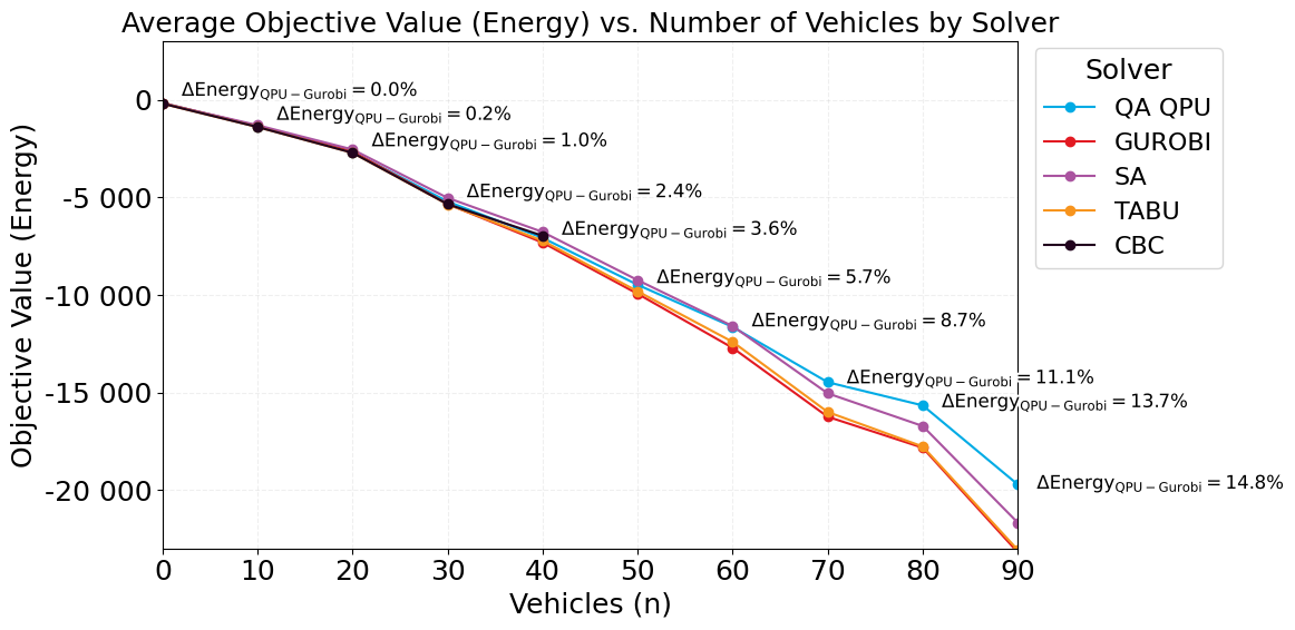
Figure 2: Average objective value (energy) versus number of vehicles ($n$) for each solver; tested for $\approx 100$ instances per $n$. Gurobi consistently returns the lowest energy, with Tabu tracking closely. SA and CBC diverge slightly as $n$ increases and QA QPU achieves the hightest energies.

Fig. 2 presents the average objective value across all simulations, plotted against the number of vehicles (rounded to the nearest ten). As the problem size increases, the objective values decrease due to the growing number of pairwise vehicle interactions encoded in the QUBO formulation. For $n\leq 30$, all solvers perform comparably, with only marginal differences in energy. From $n=40$ onward, Gurobi consistently achieves the lowest objective values, closely followed by Tabu. QA QPU, SA and CBC remain competitive but begin to diverge as $n$ increases. The relative energy difference between QA and Gurobi remains below 1% for smaller instances ($n\leq 20$), but increases steadily with problem size, reaching 15% at $n=90$.

Table 3: Proportion of simulations (%) in which each solver achieved the lowest or equal objective value. Gurobi dominates across all $n$, with QA leading a notable fraction of runs at small $n$ (rounded-up).

Vehicles ($n$)	QAQPU [%]	Gurobi [%]	SA [%]	Tabu [%]	CBC [%]
10	100.0	100.0	66.7	83.3	83.3
20	84.2	98.5	20.3	91.0	93.2
30	36.5	98.1	2.9	74.0	80.8
40	4.7	100.0	0.0	43.5	63.5
50	3.7	100.0	0.9	46.7	69.2
60	2.4	97.6	0.0	23.6	0.0
70	0.0	100.0	0.0	11.1	0.0
80	1.7	98.3	0.0	9.2	0.0
90	2.3	97.7	0.0	0.0	0.0
100	0.0	100.0	0.0	14.3	0.0

Table 4: Proportion of simulations (%) in which each solver achieved the shortest or equally long runtime. Gurobi outperforms all solvers, followed occasionally by QA and Tabu in small-$n$ cases (rounded-up).

Vehicles ($n$)	QAQPU [%]	Gurobi [%]	SA [%]	Tabu [%]	CBC [%]
10	0.0	91.7	8.3	0.0	0.0
20	1.5	98.5	0.0	0.0	0.0
30	1.9	98.1	0.0	0.0	0.0
40	0.0	100.0	0.0	0.0	0.0
50	1.0	99.0	0.0	0.0	0.0
60	2.4	96.9	0.0	0.8	0.0
70	0.0	100.0	0.0	0.0	0.0
80	1.7	98.3	0.0	0.0	0.0
90	2.3	97.7	0.0	0.0	0.0
100	0.0	100.0	0.0	0.0	0.0

To further quantify performance, we report for each solver the proportion of simulations in which it achieved either the lowest or equal objective value in Table 3, or the shortest or equally long runtime in Table 4.

The results confirm that Gurobi outperforms other solvers on small-scale instances, achieving both the lowest objective values and the shortest runtimes across nearly all test cases (in average $0.005$ seconds per instance). QA QPU also performs strongly for simulations with $n\leq 30$, where it returns feasible solutions (in 93% cases) with objective values often close to those of Gurobi. This observation aligns with previous studies demonstrating that quantum annealers can provide high-quality solutions for small, densely connected QUBOs [4]. Tabu search shows competitive behavior in early instances as well, offering a viable classical alternative in the absence of exact methods. In contrast, SA, while computationally efficient, appears less capable of navigating the complex energy landscape of dense traffic QUBOs without further schedule tuning. CBC, due to runtime constraints and increased overhead, is applicable only up to $n\leq 50$ and will not be included in further evaluations.

This analysis establishes a baseline for subsequent sections, where we investigate how solver performance evolves with increasing problem size. In particular, we anticipate performance shifts as hybrid quantum approaches are applied to medium- and large-scale instances.

4.2 Medium-scale instance analysis

We now turn to medium-scale instances with $n\leq 500$ vehicles. These experiments were conducted in larger urban areas (Prague and Košice, radius up to 0.5–1 km) characterized by higher vehicle densities and more complex routing interactions. In this scenario, we replaced the QA QPU solver with QAHS, and benchmarked its performance against Gurobi, SA, and Tabu.

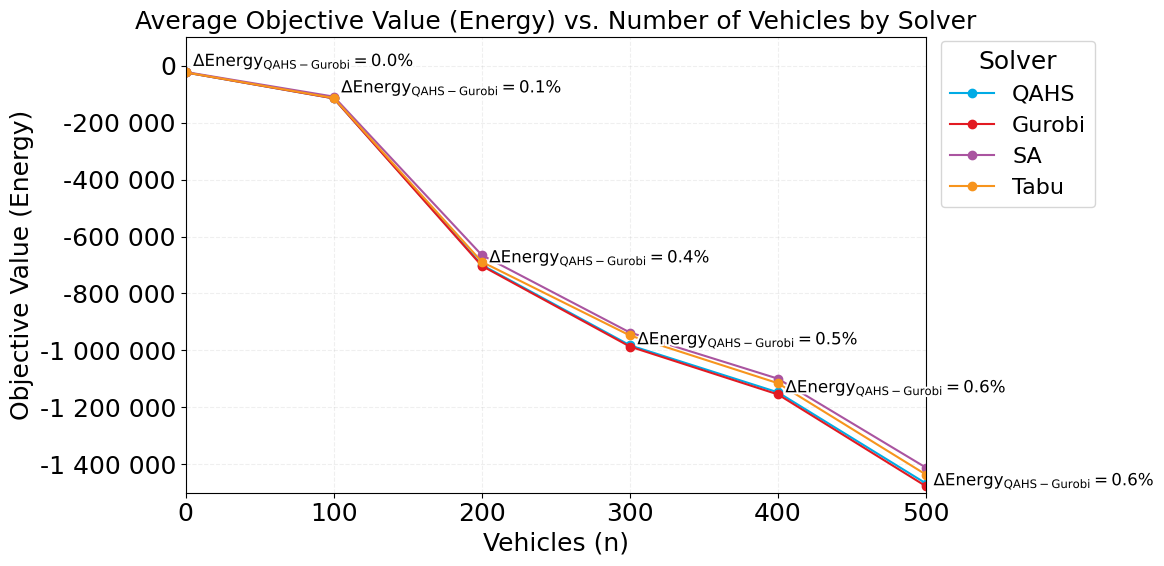
Figure 3: Average objective value (energy) versus number of vehicles ($n$) for each solver in medium-scale instances. Gurobi consistently achieves the lowest energy. QAHS tracks closely, while SA and Tabu increasingly diverge as $n$ grows.

As shown in Fig. 3, Gurobi consistently produced the best objective values across all tested sizes. QAHS closely followed, with its relative energy gap increasing gradually—from under 0.1% at $n=100$ to approximately 0.6% at $n=500$, and produced feasible solution in 100% cases. SA and Tabu, despite scaling to larger $n$, failed to yield competitive objective values. Both heuristics showed a growing divergence from the optimal trajectory as problem size increased, hence will be excluded from further evaluations in the large-scale instance analysis.

Regarding the solver runtime, Gurobi remained the fastest solver up to $n\approx 300$, with execution times ranging from milliseconds to a few seconds, depending on problem density and presolve strength. QAHS, on the other hand, exhibited a stable runtime of approximately 3 seconds across all instances. This constant-time behavior aligns with existing documentation[14] and will be futher dicsussed in Section 4.3. Tabu and SA showed significantly longer runtimes, especially at higher $n$, with Tabu exceeding 200 seconds per instance in the worst cases. Their growing computational cost, combined with declining solution quality, further supports their exclusion from subsequent experiments.

In summary, medium-scale experiments reinforce Gurobi and QAHS as the most effective solvers for realistic traffic assignment tasks formulated as QUBOs. Gurobi continues to provide optimal solutions efficiently, while QAHS offers a scalable alternative with constraint satisfaction, predictable runtime, and near-optimal performance. Classical metaheuristics such as SA and Tabu do not deliver sufficient value at this scale.

In the next section, we extend the evaluation to large-scale, real-world scenarios with thousands of vehicles, including city-wide routing toward both random and predefined destinations, which generate distinct congestion patterns.

4.3 Large-scale instance analysis

To assess solver performance at real-world scale, we evaluated over 1,500 large-scale instances with up to $n=25,\!000$ vehicles. These simulations were conducted on full city maps of Prague, Košice, and Cardiff, with vehicle routes generated randomly or directed toward attraction-based destinations. At this scale, we focused exclusively on comparing QAHS and Gurobi, since earlier results had shown that heuristic solvers do not remain competitive.

Table 5: Average QAHS performance across large-scale simulations ($n\leq 10,\!000$) rounded to thousands, evaluated on approximately 1,500 TFO instances. The last column indicates the number of simulations in which QAHS outperformed Gurobi.

Vehicles ($n$)	$\Delta\text{Energy}_{\text{QAHS - Gurobi}}$ [%]	Valid [%]	$\text{Energy}_{\text{QAHS}}<\text{Energy}_{\text{Gurobi}}$
500	0.66	100.00	237
1,000	0.63	100.00	15
2,000	0.76	100.00	0
3,000	0.80	100.00	0
4,000	0.90	100.00	0
5,000	0.90	99.98	0
6,000	0.94	99.99	0
7,000	0.98	99.98	0
8,000	0.91	99.98	0
9,000	0.88	99.99	0
10,000	0.99	99.98	0

As summarized in Table 5, QAHS maintained an average energy gap of less than 1% relative to Gurobi across all large-scale instances. In around 250 cases, mostly for $n\leq 1000$, QAHS even outperformed Gurobi. While the overall gap remained small, isolated outliers appeared in very sparse QUBOs at higher vehicle counts, where $\Delta$Energy reached up to 1.6%. Importantly, feasibility was preserved in nearly all cases, with more than 99.98% of solutions satisfying the one-hot constraints.

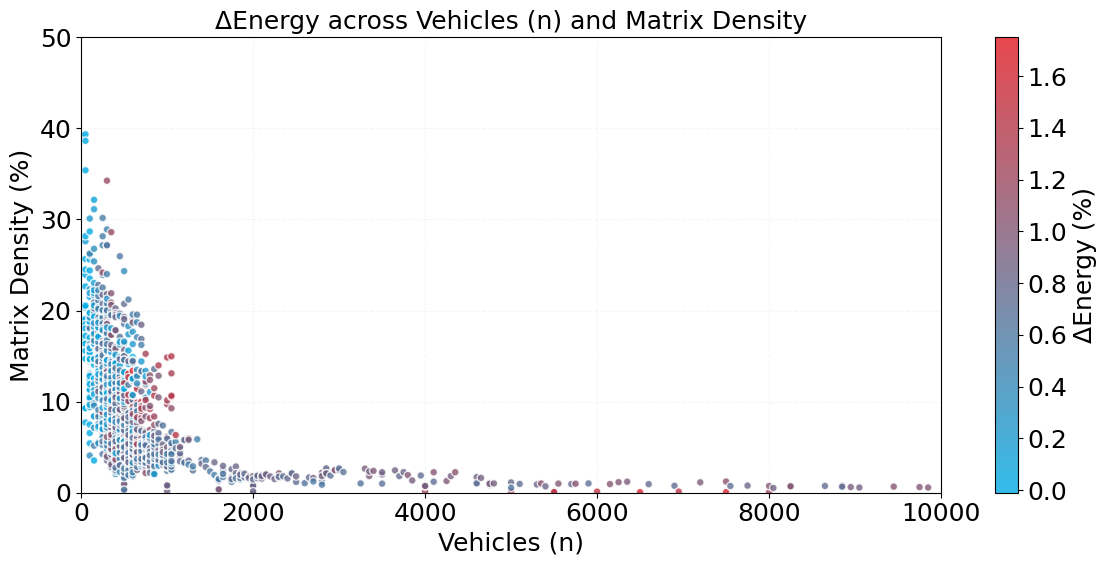
Figure 4: Relationship between solver performance and QUBO density. Each point represents a simulation, with color encoding the QAHS–Gurobi energy gap. QAHS is closest to optimal in denser formulations (blue points) and diverges modestly in sparse formulations (redder points).

The relationship between QUBO matrix density and solver performance is illustrated in Fig. 4. QAHS tracks Gurobi almost perfectly when QUBO matrices are relatively dense, but small deviations emerge as density falls below 1% at larger $n$. This behavior is consistent with the findings of Kim et al. [35], who reported that quantum annealers are most competitive on dense Hamiltonians where classical solvers struggle with quadratic growth in interactions. Conversely, sparser instances tend to favor classical methods, explaining the modest increase in $\Delta$Energy observed at the largest scales.

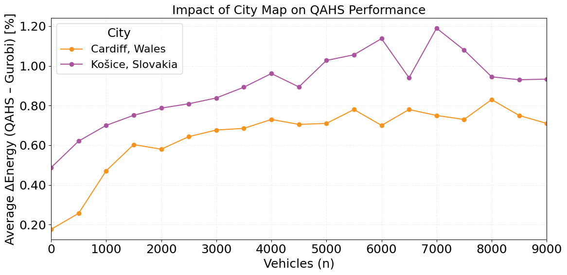
Figure 5: Comparison of solver performance across city networks. Cardiff’s uniform grid-like topology produces smaller QAHS–Gurobi gaps, while Košice’s irregular layout results in larger deviations.

Map diversity also plays a significant role. As shown in Fig. 5 and Table 7 (Appendix F), Cardiff achieves the most stable performance, with QAHS–Gurobi gaps remaining below $0.8\%$ even for large $n$, reflecting the advantages of its uniform grid-like topology. By contrast, Košice, with its irregular intersections and denser connectivity, exhibits larger gaps (exceeding $1.0\%$ for $n>5,\!000$), indicating that solver performance is more sensitive in irregular, heterogeneous networks. This is a critical observation: the QUBO graph must be embedded onto the solver’s physical graph (topology), and this embedding step often becomes the bottleneck that impacts solution quality, as also noted in [36, 14].

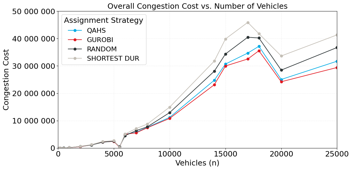
Figure 6: Comparison of congestion cost across assignment strategies (QAHS, Gurobi, random, and shortest-duration baseline). Results are aggregated over large-scale instances.

To better assess the system-wide traffic impact, we next compare solvers in terms of congestion cost (Eq. 16), a metric combining route penalties and congestion scores. Route penalties capture the extra travel time relative to the shortest option for each vehicle, while congestion scores quantify leader–follower conflicts on shared road segments. Fig. 6 shows that both QAHS and Gurobi substantially reduce congestion relative to random or shortest-duration baselines, with Gurobi generally achieving the lowest overall cost and QAHS producing near-optimal results. This provides an additional perspective: consistently assigning vehicles to their shortest-duration routes may appear optimal for individuals but, at the system level, it amplifies congestion by forcing many vehicles onto the same high-demand segments. In contrast, optimization-based approaches balance individual travel time with network-wide interactions, leading to lower overall congestion.

Table 6: Relative improvement (%) in congestion achieved by QAHS and Gurobi compared to the shortest-route baseline; tested on city map of Košice.

Vehicles ($n$)	QA vs. Shortest [%]	Gurobi vs. Shortest [%]
100	0.0	0.0
200	0.0	0.0
500	8.3	15.7
1,000	9.4	11.6
2,000	15.1	19.5
3,000	7.5	7.6
4,000	6.0	7.3
5,000	2.8	5.4
6,000	1.8	1.8
7,000	16.3	20.7
8,000	13.4	14.9
10,000	22.4	24.8
14,000	22.0	27.2
15,000	15.0	16.9
17,000	24.4	29.1
20,000	18.8	21.4
25,000	23.4	29.4

From a practical perspective, the relevance of TFO lies in its ability to reduce congestion compared to baseline routing strategies commonly used in existing navigation systems, which typically assign vehicles to either the shortest-duration or a random route. Table 6 reports the relative improvement in overall congestion when solving the TFO with QAHS and Gurobi, expressed as a percentage reduction against the shortest-route baseline. Both solvers demonstrate substantial benefits as the number of vehicles increases, with improvements up to 24,4% (QAHS) and 29.1% (Gurobi) for large-scale scenarios ($n\geq 10{,}000$). The results highlight two key insights: (i) quantum annealing can achieve improvements of a similar order to Gurobi, confirming its competitiveness for large-scale traffic assignment; and (ii) even modest improvements can lead to considerable practical benefits, as congestion increases nonlinearly with fleet size; with larger numbers of vehicles, small reductions in route overlap can prevent disproportionately large delays in the overall network.

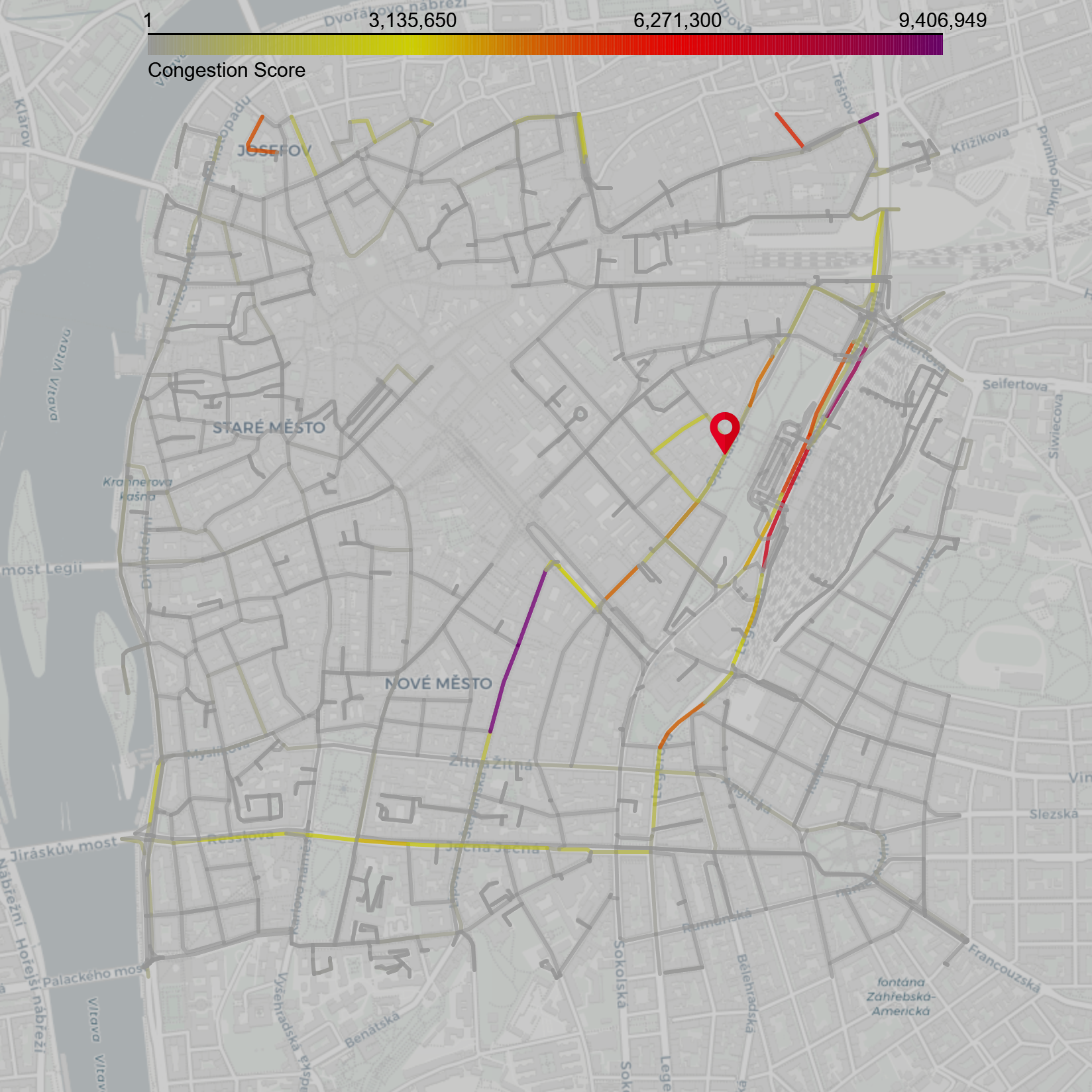
(a) Overall congestion

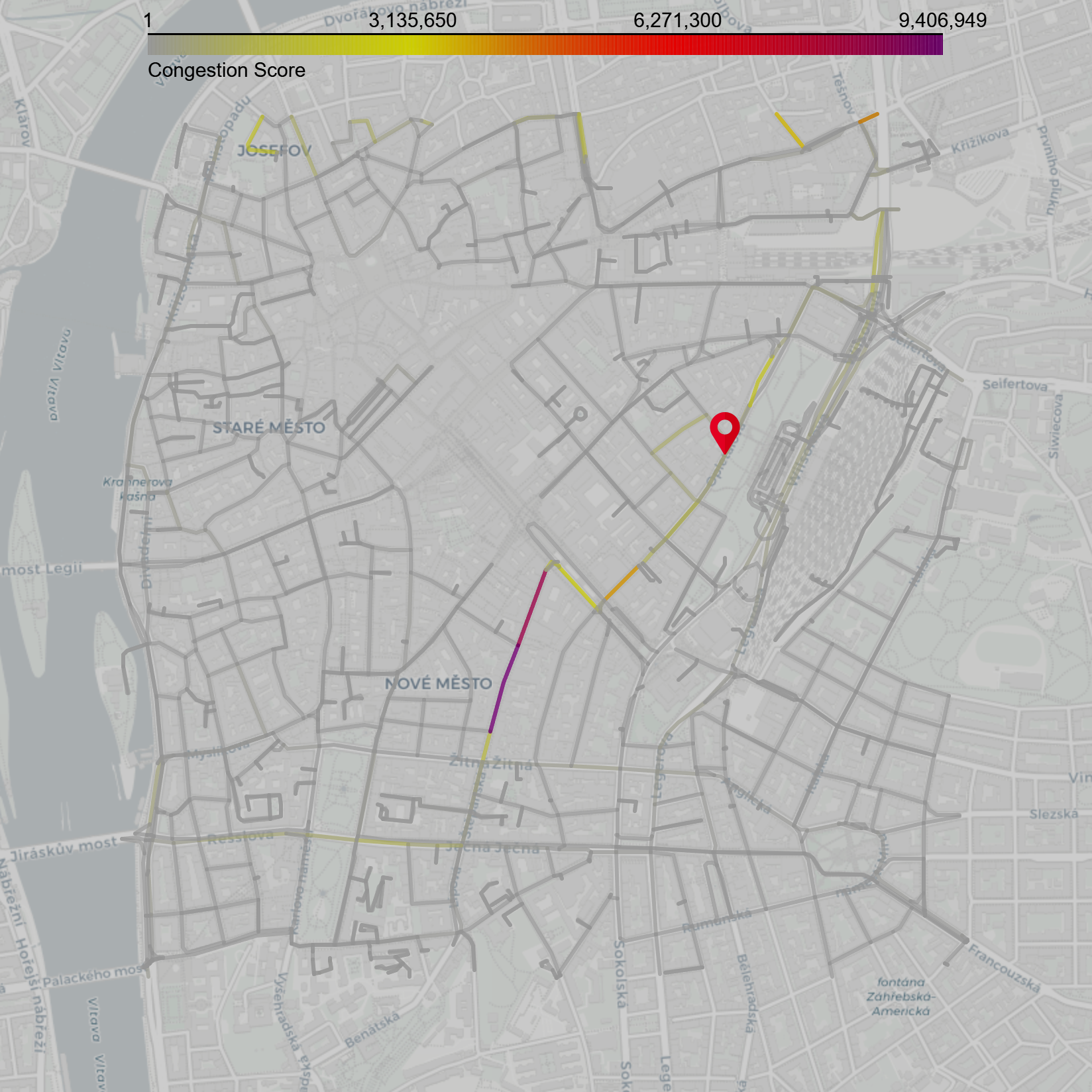
(b) Shortest (duration)

(c) QAHS assignment

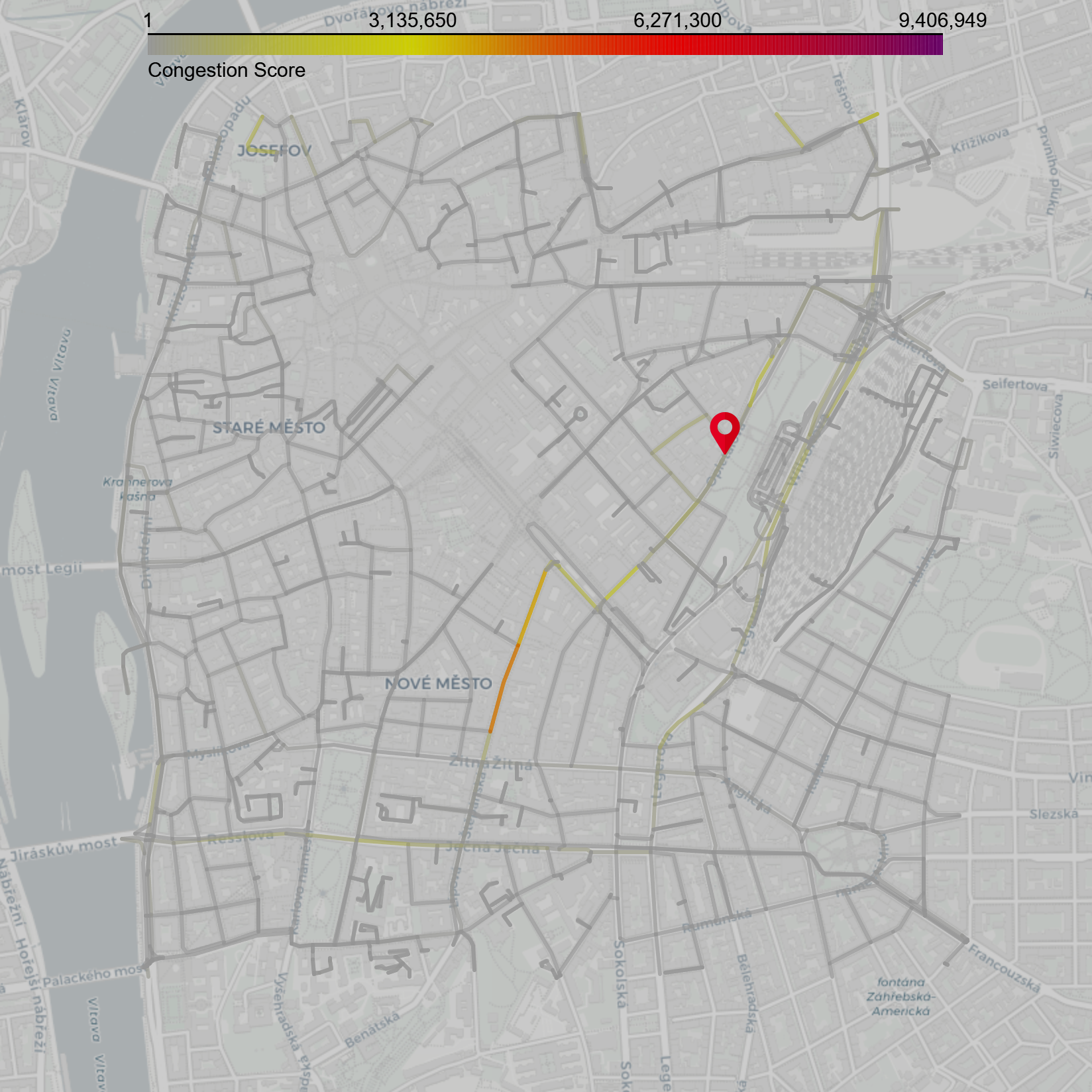
(d) Gurobi assignment

Figure 7: Congestion outcomes for a Prague instance with a single attraction point - Main Station. The problem was split into 20 clusters with an average density of 9.6%. All assignments were valid. Congestion costs: QAHS = 52,089,128; Gurobi = 50,765,774; Random = 58,948,221; Shortest = 76,398,061.

The maps in Fig. 8 illustrate how optimization changes traffic distribution. Random and shortest-duration assignments produce visibly congested corridors, whereas QAHS and Gurobi spread traffic more evenly, with Gurobi achieving slightly lower costs. The attraction-point scenario, illustrated in Fig. 7, presents a more challenging setup in which all vehicles are routed toward a common destination. Compared to the no-attraction case (Fig. 8 ), congestion patterns become more concentrated around key access corridors, amplifying localized conflicts.

(a) Overall congestion

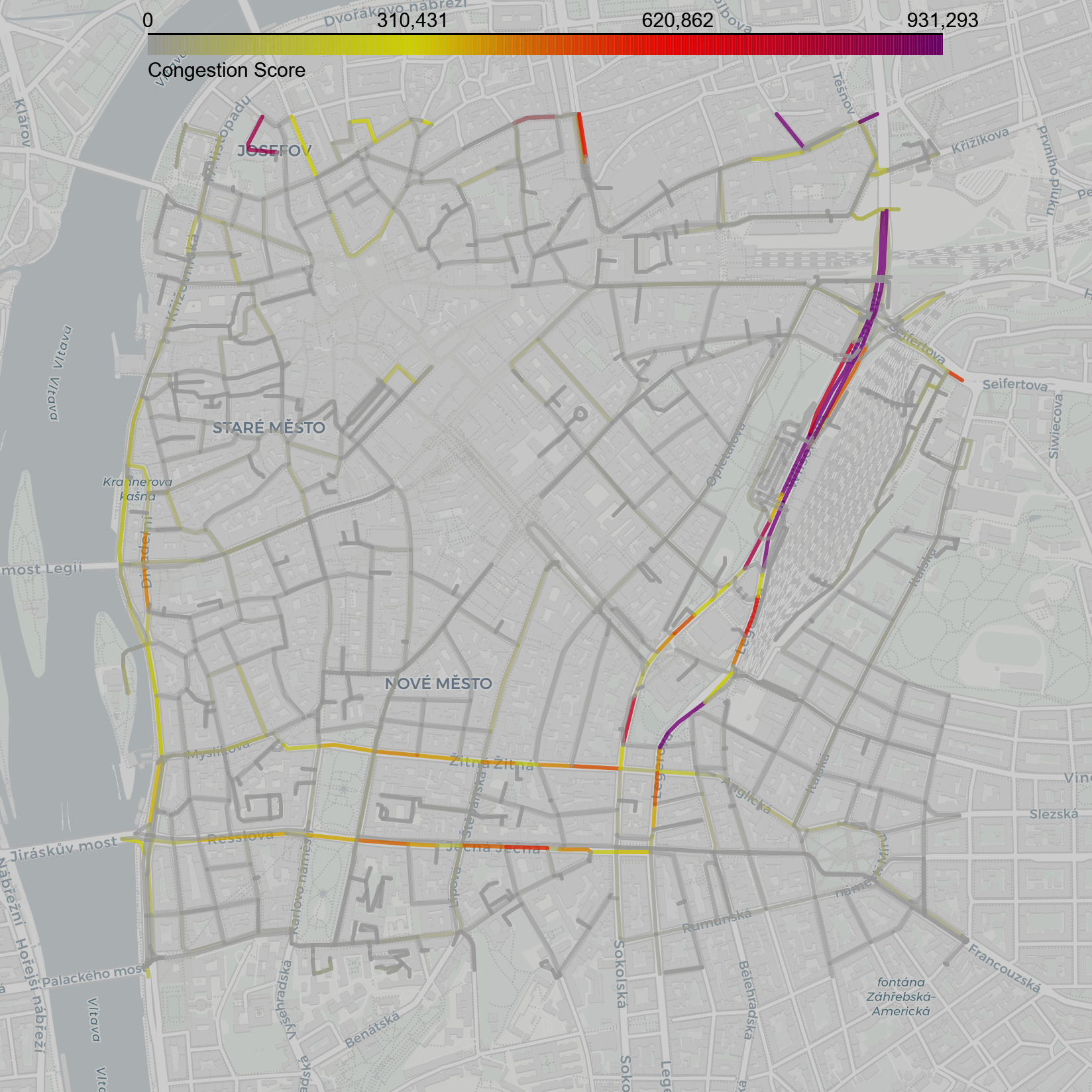
(b) Selected segments

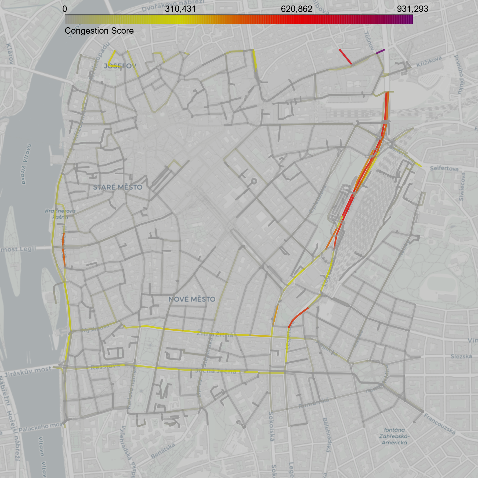
(c) Random assignment

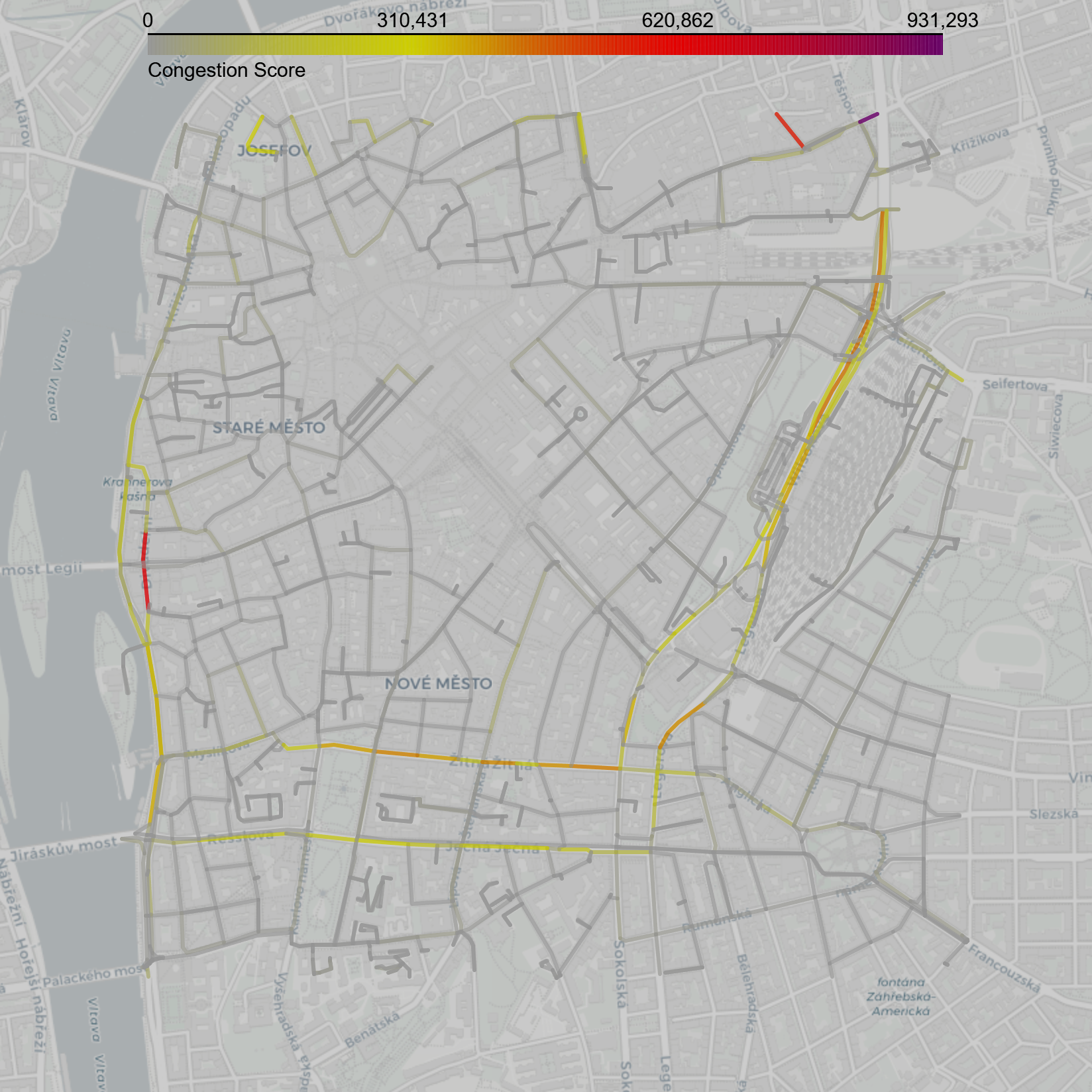
(d) Shortest (duration)

(e) QAHS assignment

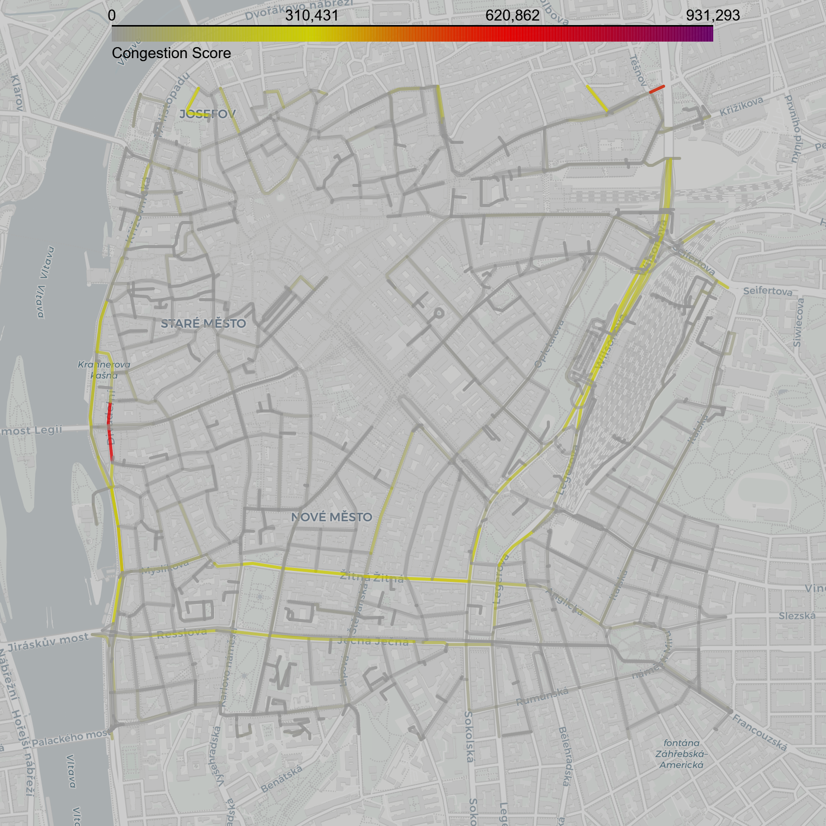
(f) Gurobi assignment

Figure 8: Visualization of congestion outcomes for a Prague instance without attraction point. The problem was split into 21 clusters with an average density of 5.6%. All assignments were valid. Congestion costs: QAHS = 20,289,324; Gurobi = 19,407,515; Random = 24,​990,​768; Shortest = 23,846,101.

While the shortest-duration baseline initially appears favorable due to its directness, it produces severe bottlenecks at the target area and ends up as the worst assignment. QAHS successfully respects all constraints and spreads traffic across alternative corridors, with only small gap compared to Gurobi’s optimized assignments. These results demonstrate that the shortest route is not necessarily the best option, since it intensifies congestion at critical locations. The TFO framework should therefore explicitly discourage such assignments in favor of overall congestion minimization.

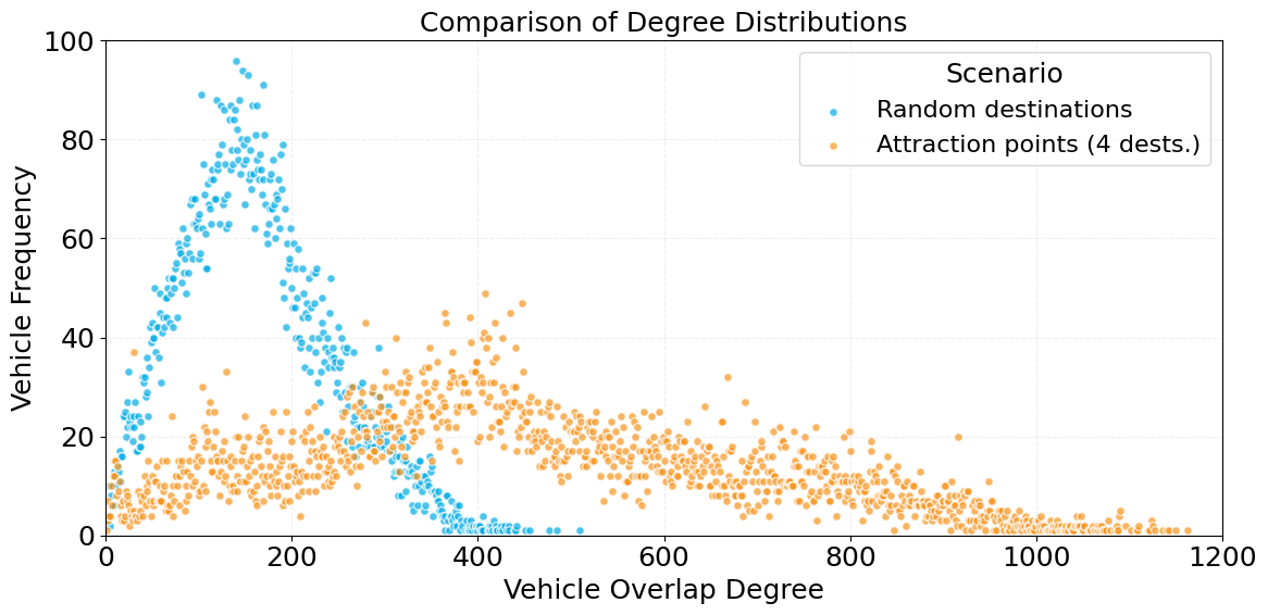
Figure 9: Degree distribution of the Prague network under two scenarios, showing vehicle frequency by overlap degree. Random destinations (blue) produce a narrow distribution concentrated at lower degrees ($<300$), indicating localized and relatively evenly spread congestion. Attraction points (orange, 4 dests.) yield a much broader distribution extending beyond 1,000 degrees, demonstrating how common destinations amplify vehicle interactions and generate long-tailed congestion patterns.

Fig. 9 further highlights how attraction points alter vehicle interactions. While the random assignment produces relatively homogeneous distribution of congestion, the attraction-point scenario introduces widespread structural congestion with a heavy-tailed distribution in which some vehicles overlap with more than one thousand others. This indicates that traffic converging toward a limited set of destinations generates hub-like vehicles that accumulate disproportionately high congestion. Such heavy-tailed patterns are consistent with empirical findings in real-world traffic systems, where congestion cluster sizes and durations follow scaling laws rather than uniform distributions [20, 37]. From Figs. 8 and 7, we also observe that both QAHS and Gurobi solvers handle this increased complexity with comparable performance, as the difference in their congestion costs increase almost equally ($+31.8$M vs. $+31.4$M).

The runtime analysis reveals important differences between quantum and classical solvers, Table 8 (Appendix F). Gurobi consistently outperforms QAHS for smaller problem sizes ($n\leq 4000$), often completing in less than half the time. However, for larger instances, runtimes converge due to a fixed wall-clock limit aligned with QAHS runtime. The QAHS solver exhibits highly predictable timing behavior, with runtime increasing almost linearly with problem size, i.e., the number of subproblems generated during decomposition [38], from just 3 seconds at $n=0$ to approximately 117 seconds at $n=10{,}000$. This predictability makes QAHS attractive for near real-time deployment, where consistent latencies are often more valuable than guaranteed optimality.

Importantly, QPU access time (the actual time spent on the QPU) remains negligible (below 0.1 seconds across all sizes), confirming that the bottleneck lies in orchestration, problem embedding, and postprocessing. These overheads include the programming cycle, thermal stabilization, and communication with classical controllers. Even small problems incur similar initialization costs, which explains the nearly fixed baseline runtime[39].

Regarding the model preparation time, which is executed locally, Gurobi’s translation of QUBO to MILP is relatively lightweight, whereas QAHS requires converting the QUBO into a Binary Quadratic Model (BQM). This step introduces additional object construction and normalization overhead and can take up to twice as long as Gurobi MILP-preparation.

Nonetheless, unlike classical MILP solvers such as Gurobi, whose worst-case runtime grows exponentially with problem size (e.g., due to branch-and-bound search, i.e., $O(2^{n})$) [18], QAHS maintains more stable empirical scaling by distributing workloads into independent subproblems. This combination of scalability and timing consistency positions QAHS as a practical tool for large-scale traffic optimization, where runtime guarantees may outweigh provable optimality, especially given that in the TFO setting the observed optimality gap was below 1% and further depends on the specific structure of the underlying city map (Fig. 5).

5 Discussion

The TFO framework demonstrates that the QUBO formulation is a particularly promising candidate for representing congestion-aware routing. By directly aligning with the structure of D-Wave annealers, QUBO formulations capture the interaction of vehicles at a fine-grained spatial and temporal resolution, allowing congestion to be modeled with a level of realism that exceeds many simplified traffic assignment approaches. This granularity is one of the principal strengths of the method, enabling the solver to identify overlaps that would be overlooked in more aggregated formulations.

At the same time, the detailed treatment of congestion introduces practical limitations. Because every pairwise conflict must be stored in the database and incorporated into the QUBO, matrix construction can become a bottleneck. On a local machine, preparing the QUBO and computing congestion weights required several minutes, and for the largest problem sizes this preparation extended to almost ten minutes. The framework thus balances realism against preparation overhead, highlighting the importance of efficient preprocessing when scaling to city-wide deployments.

A key advantage of the proposed workflow is its adaptability. If a junction is reported, the corresponding road segments can be excluded dynamically from the optimization graph. The same holds for traffic accidents: information obtained from services such as Waze can be used to discard affected points and adjust adjacent segments, thereby ensuring that emergency services retain clear access while the remaining traffic is rerouted in real time.

The framework also supports proactive scenario modeling. Anticipated events such as concerts or sporting games can be simulated in advance, thereby revealing which corridors will be most affected and enabling authorities to prepare appropriate mitigation strategies.

The applicability of the TFO framework extends further into autonomous mobility. In conventional traffic, only a portion of drivers follow navigation recommendations, limiting the impact of global optimization. By contrast, in a setting where all autonomous vehicles adhere to congestion-aware assignments simultaneously, the system-wide benefits are amplified.

While the present formulation optimizes congestion reduction and travel time, it can be extended to incorporate additional dimensions of realism. Road capacity thresholds could be introduced as penalties once certain flows exceed physical limits, while waiting times at traffic signals could be added to capture intersection delays. Such enrichments may become feasible with future hardware advances, as improvements in connectivity and qubit reliability could open the way for handling more complex formulations more effectively.

Taken together, the present study demonstrates not only a competitive quantum–hybrid approach for solving large-scale TFO but also a versatile modeling framework. Its ability to adapt dynamically to accidents, closures, or planned events, combined with the prospect of integration into autonomous mobility systems, highlights its potential for real-time traffic management.

Conclusion

Our results show that hybrid quantum annealing delivered solutions within 1% of state-of-the-art classical solver, while keeping runtimes stable and solutions almost always feasible. This points to a practical stage of quantum readiness, where hybrid quantum approaches are not just theoretical but already competitive in solving real optimization challenges such as large-scale traffic flow optimization. Compared to shortest-path routing, our method reduces congestion by up to 25%, highlighting a clear benefit for system-wide mobility management.

For urban transport, these findings suggest that quantum-enhanced optimization could complement existing navigation services by providing congestion-aware route assignments. Unlike commercial platforms that primarily optimize individual travel times, our QUBO-based formulation balances driver efficiency with global congestion reduction. This positions the framework as a promising addition to future ITS, where integration with live mobility data could help anticipate hotspots, smooth traffic flow, and improve the use of road networks. While much prior work has focused on small test cases or iterative refinements of QUBO models, our study demonstrates that quantum methods can already scale to realistic city networks with up to 25,000 vehicles. Moreover, the experiments highlight sensitivity to network topology, with Cardiff showing a gap as low as 0.8%, underlining the importance of map diversity in performance evaluation.

Looking ahead, advances in quantum hardware, solver connectivity, and embedding techniques are expected to expand the scale and quality of problems solvable directly on quantum devices. In the context of Traffic Flow Optimization, however, our results also reveal the current hardware limits of the D-Wave system, which constrain both the maximum instance size and the quality of solutions. These constraints are problem dependent, as different city topologies and formulations challenge the hardware in distinct ways.

Appendix A Parameter selection

A.1 Penalty parameter

The penalty parameter $\lambda$ plays a central role in our formulation, since it directly influences both the quality of the solutions and how efficiently solvers perform [40, 41, 42]. If $\lambda$ is chosen too small, the solver may return infeasible assignments where vehicles are given multiple routes. On the other hand, if $\lambda$ is too large, the penalty term overwhelms the objective, masking the trade-offs between travel time and congestion.

Different strategies for choosing $\lambda$ have been proposed. In their Mini-scale traffic flow optimization study, Salloum et al. [10] set $\lambda$ equal to the maximum iteration cost of a vehicle–route assignment. This is conceptually close to our approach, although their formulation was restricted to a single route per vehicle.

García et al. [43] introduced three exact approaches to compute valid penalty weights in QUBO: (i) the sum of absolute coefficients method, which derives an upper bound on the smallest valid penalty by summing positive and negative contributions in the QUBO polynomial; (ii) the posiform/negaform transformation, which rewrites the QUBO into equivalent forms with only non-negative or non-positive coefficients, yielding tighter bounds; and (iii) the Verma–Lewis method, which evaluates row-wise sums of coefficients to obtain the tightest valid weights. All three methods guarantee feasibility preservation but the Verma–Lewis[44] method consistently provided penalty weights closest to the best known.

In our formulation, we follow the Verma–Lewis principle. Since our QUBO matrix $\mathbf{Q}$ is stored in upper-triangular form, these row-wise sums are obtained (directly during QUBO construction) by aggregating coefficients across rows and columns, see Alg. 2.

A.2 Sensitivity parameter

In the congestion score (Eq. 3), the parameter $\gamma$ controls the sensitivity of the model to vehicle spacing. It scales the ratio $\tfrac{d}{\bar{v}}$, which represents the time headway—a standard measure used in traffic safety and leader–follower dynamics.

By setting $\gamma\in[2,4]$, we restrict interactions to vehicles traveling within approximately $2$–$4$ seconds of one another. This interval is consistent with empirical evidence and microscopic traffic models such as the Intelligent Driver Model, which typically calibrate desired headways in the range of $1.5$–$2.5$ seconds [45, 46]. Moreover, road safety guidelines promote the “two-second rule” (extended to $3$–$4$ seconds in adverse conditions) [47], further justifying this parameter choice.

Appendix B Construction of QUBO matrix

Algorithm 2 Construction of QUBO matrix $\mathbf{Q}$

Input: Vehicle set $C$, uniform alternatives $k$, congestion weights $w_{i,j,a_{i},a_{j}}$, duration penalties $\pi_{i,a_{i}}$

Output: QUBO matrix $\mathbf{Q}$, penalty parameter $\lambda$

Map each $(i,a_{i})$ to a unique QUBO index $q_{i,a_{i}}$;

Identify the set of vehicles $i$ for which less then $k$ routes was generated and create set of ”not-real” route alternatives and set of corresponding indices $\mathcal{N}$.

Initialize empty QUBO $\mathbf{Q}\leftarrow\{\}$

Add congestion weights:

for each pair of vehicles $i<j$ do

  for each $a_{i}\in\{1,\dots,k\}$ do

   for each $a_{j}\in\{1,\dots,k\}$ do

     $\mathbf{Q}[q_{i,a_{i}},\,q_{j,a_{j}}]+=w_{i,j,a_{i},a_{j}}$

   end for

  end for

end for

Compute $\lambda$:

Calculate $\Lambda_{i,a_{i}}$ via Eq. 9

Set $\lambda=\max_{i,a_{i}}\Lambda_{i,a_{i}}$

Add penalties:

for each vehicle $i\in C$ do

  for each distinct pair $a_{i}\neq b_{i}$ do

   $\mathbf{Q}[q_{i,a_{i}},\,q_{i,b_{i}}]+=\lambda$ $\triangleright$ one-hot off-diagonal

  end for

end for

for each index $q_{i,a_{i}}$ do

  if $q_{i,a_{i}}\in\mathcal{N}$ then

   $\mathbf{Q}[q_{i,a_{i}},\,q_{i,a_{i}}]+=\lambda$ $\triangleright$ not-real route: discourage selecting

  else

   $\mathbf{Q}[q_{i,a_{i}},\,q_{i,a_{i}}]+=-\,\lambda\;+\;\pi_{i,a_{i}}$ $\triangleright$ real route: constraint + duration penalty

  end if

end for

Output $\mathbf{Q}$ as solver input

Appendix C Solvers details

Quantum Annealing. D-Wave Systems provides cloud-based access to quantum annealing hardware optimized for QUBO problems [21]; access is programmatic via the Python Ocean SDK through the Leap service, where users authenticate with a Leap API token [22].

In quantum annealing, the problem is encoded as the ground state of an Ising Hamiltonian, with binary variables represented by qubits. The quantum system is evolved adiabatically from an easily prepared initial state toward the target Hamiltonian, ideally remaining in the ground state throughout. Connectivity constraints in the hardware require minor-embedding, which is itself NP-hard and performed classically before annealing [48]. The Advantage QPU employs the Pegasus topology, featuring approximately 5,640 qubits in its main fabric (5,760 total) and up to 15 connections per qubi offering significantly enhanced connectivity over the older Chimera topology ($\sim$6 connections per qubit) [49]. This increased connectivity allows fully connected problem embeddings of up to $\sim$177 logical variables [50, 51], though in practice any required chains of physical qubits become long and fragile at this scale. By contrast, the more recent Advantage2 system uses the Zephyr topology, with around 4,400 physical qubits and 20-way connectivity allowing fully connected embeddings of up to $\sim$280 logical variables [52]. D-Wave’s cloud platform also provides hybrid solvers for larger problems. The LeapHybridBQMSampler handles unconstrained binary quadratic models by combining the quantum annealer with classical heuristics (embedding penalty terms directly into the objective). The LeapHybridCQMSampler supports constrained quadratic models with one-hot constraints enforced directly (avoiding manual penalty tuning and improving feasibility), but we did not use the CQM solver due to its significantly longer runtime. [53]

Gurobi. Gurobi is an industry-grade commercial solver for mixed-integer programming [23]. It employs a linear-programming-based branch-and-bound algorithm with cutting-plane enhancements, as originally introduced by Land and Doig [24]. Problems formulated as QUBO can be solved by reformulating them as MILPs with auxiliary variables for quadratic terms directly using Gurobi’s model properties. Though this increases the problem size, it enables expressing the model in a structure comparable to the other solvers and serves as a transparent, exact solver for linearized QUBOs under the same one-hot constraints and objective function.

For our simulations, we use Gurobi via the Python gurobipy package distributed on PyPI [25], running under a free academic license through the Gurobi Web License Service (WLS) [54]. A per-instance solver execution time limit is set to our quantum annealing solver runtime dynamically for each problem instance. In this setting, Gurobi provides a reliable exact baseline against which the solutions produced by quantum annealing can be compared in terms of both quality and scalability.

CBC. The COIN-OR Branch-and-Cut (CBC) solver [26] is an open-source MILP solver built on a branch-and-bound framework enhanced by cutting planes. Because CBC does not natively support quadratic terms, we manually linearize the QUBO by introducing auxiliary binaries (similarly to our Gurobi setup).

We accessed CBC through the PuLP Python library [27] and executed it locally. In practice, however, CBC struggled with medium- or large-scale instances and was viable only for small-scale testing. Consequently, we used it mainly as a license-free baseline for exact optimization.

Simulated Annealing. Simulated Annealing (SA) provides a classical stochastic baseline for QUBO solving. Inspired by the physical cooling process of materials the algorithm searches the solution space by applying local modifications: while improvements are always taken, non-improving moves can also be accepted with a probability that decreases as the system “cools“. This mechanism helps the algorithm escape local minima and approximate global optima [28, 55].

We implemented SA using D-Wave’s open-source neal library, where the QUBO matrix is converted into a binary quadratic model and sampled with default parameters [29]. While SA runs quickly and locally, it does not provide optimality guarantees and is better suited as a lightweight classical baseline than a scalable solver. Hence, we used it only to benchmark small-sale instances of TFO.

Tabu Search. Tabu Search (Tabu) is a metaheuristic that enhances local search with short-term memory to avoid cycling. Rather than repeatedly revisiting recent solutions, it maintains a dynamic “tabu list” of forbidden moves for a specified tenure, meaning that a move remains disallowed for a fixed number of iterations before it can be reconsidered. This mechanism helps steer the search toward unexplored neighborhoods and balances intensification around promising solutions with diversification into new regions [30, 56].

For our testing, we used D-Wave’s dwave-tabu sampler [31, 32] with default parameters, which applies tabu-based local search directly to binary quadratic models. While tabu search cannot guarantee optimality, it is lightweight, runs locally, and often produces strong heuristic solutions for QUBO problems. Similar to SA, we employed it only for small-scale instances of TFO, as computation times grew significantly with larger problem sizes.

Appendix D Leiden Clustering

To partition the congestion graph into smaller subproblems, we apply the Leiden community detection algorithm [1]. The choice of Leiden is motivated by both practical and theoretical considerations. Feld et al. [57] showed that attempting clustering using QUBO is unstable, requires dataset-specific penalty tuning, and often fails to respect capacity constraints and used classical k-means method on VRP. Borowski et al. [58] formalized this principle into a hybrid approach (DBSCAN Solver), where classical decomposition/clustering prepares subproblems that quantum annealing can then solve efficiently. These studies highlight that classical preprocessing is not merely a fallback, but a deliberate design choice in hybrid quantum-classical optimization pipelines.

Leiden algorithm optimizes modularity while guaranteeing well-connected clusters, making it more robust than earlier approaches such as Louvain. The resolution parameter $\rho$ (see Table 1 controls clusters granularity: higher values produce many small, dense clusters, while lower values yield fewer, larger clusters.

Small clusters below the minimum threshold are merged into neighboring communities with which they share the strongest inter-cluster edge weights. Any residual small clusters are batched together to ensure that all subproblems satisfy the minimum cluster size $m$. This merging process prevents solvers from being overloaded with numerous trivial subproblems. In our implementation, the parameter $L$ additionally allows us to control the maximum number of clusters prepared for the downstream workflow.

Each cluster $C_{\ell}\subseteq C$ with $|C_{\ell}|$ vehicles defines an independent QUBO instance of size $|C_{\ell}|\cdot k$ variables. These subproblems are solved separately using QAHS and classical optimizers. Vehicles outside all clusters (e.g., with negligible interactions) are directly assigned their shortest-duration route. Finally, the local cluster solutions are merged, and total congestion is recomputed across the full city network. While this decomposition sacrifices strict global optimality, it preserves the most critical congestion dynamics and enables comparative benchmarking across solvers with widely varying resource capacities.

Without clustering, the QUBO formulation requires $O(n^{2}k^{2})$ pairwise terms, since every vehicle–route pair may interact with every other. By partitioning the vehicle set into $L$ clusters $\{C_{1},\dots,C_{L}\}$, the effective complexity is reduced to

$$O\!\Big(\sum_{\ell=1}^{L}|C_{\ell}|^{2}k^{2}\Big),$$ (18)

which is significantly smaller whenever clusters are well-balanced and $|C_{\ell}|\ll n$. For example, with $n=25{,}000$ vehicles and $k$ route alternatives, the unconstrained formulation contains on the order of $n^{2}k^{2}\approx 6.25\times 10^{8}k^{2}$ pairwise terms. If the vehicles are partitioned into $L=25$ balanced clusters of size $|C_{\ell}|=1{,}000$, then the total complexity reduces to $25\cdot(1{,}000^{2})k^{2}=2.5\times 10^{7}k^{2}$ terms. This represents a reduction by a factor of about $25$, i.e., roughly one order of magnitude.

Thus, clustering not only keeps subproblems within solver limits, but also provides near-quadratic reductions in computational effort. This decomposition serves as a practical bridge between the theoretical formulation of the TFO and the capacity limits of applied solvers, ensuring that optimization remains feasible for large-scale instances while preserving the most critical congestion scenarios.

Appendix E Description of Overall Workflow

1. City map generation. The road network is extracted from OpenStreetMap, either by specifying a city name or by also providing a center coordinate with a radius to restrict the network to a specific subgraph. This flexibility enables simulation of diverse scenarios, from entire metropolitan areas to localized regions of interest. Experiments were conducted on multiple cities (Košice, Prague, Cardiff) and their subnetworks to demonstrate the generality of the approach.

2. Vehicles generation. Vehicles are generated with origin–destination pairs either randomly distributed or directed toward attraction point $C_{\text{att}}$. The number of vehicles is set via a parameter, and origin–destination pairs are further constrained by user-defined minimum and maximum lengths ($L_{\min},L_{\max}$), computed as geodesic (air-line) distances between the selected points.

3. Vehicle route alternatives. For each vehicle, $k$ alternative routes are calculated using the open-source Valhalla routing engine [2]. To make the routes usable for congestion modeling, they are sampled every $\alpha$ seconds to create a sequence of route points. Each point records the vehicle’s position, speed, direction, and the closest road segment, so that interactions between vehicles can be tracked in space and time. For every route we also store summary values such as total distance and travel time. Routes are fetched from Valhalla in batches using asynchronous requests, and the results are processed in parallel, which makes it possible to scale the workflow to thousands of vehicles.

4. Congestion modeling. At each time step, vehicles traveling on the same road segment and in the same direction are grouped, and leader–follower pairs are identified. For every such pair, the distance between vehicles is computed using the haversine formula (Eq. 2), which accounts for the Earth’s curvature. This distance is then normalized by their average speed and scaled by a sensitivity distance factor $\gamma$, producing a congestion score (Eq. 3) that increases when fast-moving vehicles remain close together. Scores are accumulated across all edges and time steps within the simulation window $w$ to obtain per-edge congestion entries (Eq. 4), which are stored in the database and later aggregated into pairwise congestion weights $w_{i,j,a_{i},a_{j}}$ (Eq. 5) used for the QUBO formulation.

5. Clustering (optional). For large instances, a congestion graph is constructed and partitioned using the Leiden algorithm ($\rho$ - cluster resolution) to ensure that subproblems remain within solver limits. Vehicles outside clusters or in residual groups are assigned their shortest-duration route. In rare cases where a solver returns an invalid assignment (e.g., no valid one-hot selection across $k$ routes), the vehicle is also assigned its shortest route. Although such situations are uncommon, this fallback ensures that every vehicle receives a valid route and the workflow remains consistent.

6. Optimization (QUBO solvers). For each cluster (or the full instance when clustering is not applied), a QUBO formulation is constructed and solved using a range of approaches. Depending on the problem size (see Section 3.4), this includes direct execution on the D-Wave QPU for small-scale cases, the D-Wave QAHS for medium- and large-scale instances, and classical methods: Gurobi, CBC, Simulated Annealing, and Tabu Search. The motivation and setup of each solver are described in detail in Appendix C, ensuring that quantum, hybrid, and classical baselines are compared on the same reproducible QUBO instances.

7. Evaluation and baselines. Optimized assignments are merged and total congestion is recomputed across the full network to ensure comparability between clustered and non-clustered vehicles. Results are then benchmarked against multiple baselines, including shortest-duration and random-route assignments. For each solver and baseline, we calculate congestion cost (Eq 16), solver computational duration, and assignment validity (see Subsection 3.5). All metrics and solver outputs are written to the MariaDB database, and aggregated SQL queries are used to derive joint statistics across solvers. This step provides a unified basis for comparing solver performance at different scales and under different simulation setups.

8. Analysis and visualization. Heatmaps and summary tables are produced to illustrate both city-wide congestion patterns and solver-specific outcomes. Congestion maps highlight affected road segments before and after optimization, enabling visual comparison of baselines and optimized assignments. Summary tables report solver runtimes, objective values, and congestion reductions in a standardized format across all solvers and instance sizes. This step provides both an intuitive interpretation of traffic dynamics and a structured basis for quantitative comparison.

Appendix F Additional Tables

Table 7: Minimum, maximum, and average $\Delta$Energy between QAHS and Gurobi for Cardiff and Košice. Vehicles $n$ are rounded-up.

	Cardiff, Wales			Košice, Slovakia
Vehicles ($n$)	Min	Max	Avg	Min	Max	Avg
100	0.00%	0.67%	0.18%	0.00%	6.54%	0.49%
500	0.00%	0.80%	0.26%	0.00%	1.10%	0.62%
1000	0.19%	0.61%	0.47%	0.27%	0.97%	0.70%
1500	0.53%	0.74%	0.60%	0.50%	0.99%	0.75%
2000	0.58%	0.58%	0.58%	0.61%	0.93%	0.79%
2500	0.58%	0.72%	0.64%	0.72%	1.00%	0.81%
3000	0.60%	0.73%	0.68%	0.68%	1.03%	0.84%
3500	0.68%	0.69%	0.69%	0.78%	0.98%	0.89%
4000	0.73%	0.73%	0.73%	0.74%	1.21%	0.96%
4500	0.68%	0.73%	0.71%	0.76%	1.05%	0.89%
5000	0.62%	0.79%	0.71%	0.91%	1.31%	1.03%
5500	0.78%	0.78%	0.78%	0.80%	1.58%	1.06%
6000	0.70%	0.70%	0.70%	1.00%	1.47%	1.14%
6500	0.78%	0.78%	0.78%	0.94%	0.94%	0.94%
7000	0.75%	0.75%	0.75%	0.96%	1.42%	1.19%
7500	0.73%	0.73%	0.73%	1.08%	1.08%	1.08%
8000	0.83%	0.83%	0.83%	0.87%	1.02%	0.95%
8500	0.75%	0.75%	0.75%	0.93%	0.93%	0.93%
9000	0.71%	0.71%	0.71%	0.88%	0.97%	0.93%

Table 8: Runtime comparison between QAHS and Gurobi for increasing number of vehicles. Durations are in seconds.

	QAHS		Gurobi
Vehicles ($n$)	Model preparation	Solver runtime	Model preparation	Solver runtime
100	15.07	2.99	0.87	0.62
500	29.15	3.19	3.25	1.40
1,000	42.17	4.80	9.68	3.10
1,500	69.04	7.30	20.06	3.93
2,000	93.16	9.58	34.05	6.26
2,500	131.28	14.01	53.81	9.59
3,000	176.54	18.31	75.93	15.37
3,500	252.98	24.29	111.99	23.00
4,000	320.37	28.77	142.98	25.37
4,500	421.54	35.31	200.09	35.37
5,000	476.25	39.02	206.91	32.49
6,000	709.53	53.29	313.61	43.15
7,000	944.36	70.23	409.87	46.67
8,000	1214.80	84.33	566.97	84.46
9,000	1517.65	100.38	717.93	100.51
10,000	1841.23	116.80	860.79	116.94

References

- [1] V. A. Traag, L. Waltman, and N. J. van Eck, “From louvain to leiden: guaranteeing well-connected communities,” Scientific Reports, vol. 9, p. 5233, 2019.
- [2] Mapbox, “Valhalla: Open source routing engine,” https://valhalla.readthedocs.io, 2025, accessed: 2025-08-27.
- [3] M. Q. Mohammed, H. Meeß, and M. Otte, “Review of the application of quantum annealing-related technologies in transportation optimization,” Quantum Information Processing, vol. 24, no. 9, p. 296, 2025.
- [4] F. Neukart, G. Compostella, T. Seidel, D. von Dollen, S. Yarkoni, and B. Parney, “Traffic flow optimization using a quantum annealer,” Frontiers in ICT, vol. 4, no. 29, p. 29, 2017.
- [5] S. Yarkoni, F. Neukart, E. M. Gomez Tagle, N. Magiera, B. Mehta, K. Hire, S. Narkhede, and M. Hofmann, “Quantum shuttle: traffic navigation with quantum computing,” in Proceedings of the 1st ACM SIGSOFT International Workshop on Architectures and Paradigms for Engineering Quantum Software (APEQS 2020), 2020, pp. 22–30.
- [6] J. Villanueva, G. J. Mooney, B. R. Bardhan, J. Ghosh, C. D. Hill, and L. C. L. Hollenberg, “Hybrid quantum optimization in the context of minimizing traffic congestion,” 2025, preprint at https://arxiv.org/abs/2504.08275.
- [7] M. Leib, F. Neukart et al., “An optimization case study for solving a transport robot scheduling problem on quantum-hybrid and quantum-inspired hardware,” Scientific Reports, vol. 13, no. 1, p. 20602, 2023.
- [8] H. Hussain, M. B. Javaid, F. S. Khan, A. Dalal, and A. Khalique, “Optimal control of traffic signals using quantum annealing,” Quantum Information Processing, vol. 19, no. 9, p. 312, 2020.
- [9] A. Singh, C.-Y. Lin, C.-I. Huang, and F.-P. Lin, “Quantum annealing approach for the optimal real-time traffic control using qubo,” in 22nd International Conference on Software Engineering, Artificial Intelligence, Networking and Parallel/Distributed Computing (SNPD), 2021, pp. 85–92.
- [10] H. Salloum, S. Zhanalin, A. A. Badr, and Y. Kholodov, “Mini-scale traffic flow optimization: an iterative qubos approach converting from hybrid solver to pure quantum processing unit,” Scientific Reports, vol. 15, no. 1, p. 22904, 2025.
- [11] T. Tambunan, A. Suksmono, I. Edward, and R. Mulyawan, “Quantum annealing for vehicle routing problem with weighted segment,” 2022, preprint at https://arxiv.org/abs/2203.13469.
- [12] U. Azad, B. K. Behera, E. A. Ahmed, P. K. Panigrahi, and A. Farouk, “Solving vehicle routing problem using quantum approximate optimization algorithm,” IEEE Transactions on Intelligent Transportation Systems, vol. 24, no. 7, pp. 7564–7573, 2023.
- [13] M. Cattelan and S. Yarkoni, “Modeling routing problems in qubo with application to ride-hailing,” Scientific Reports, vol. 14, no. 1, p. 19768, 2024.
- [14] D. Chitty, J. Charles, A. Moraglio, and E. Keedwell, “Applying a quantum annealer to the traffic assignment problem,” in Proceedings of the Genetic and Evolutionary Computation Conference (GECCO ’24), 2024, pp. 814–822.
- [15] K. Wheeler, “Project green light: Google using ai for sustainability,” https://aimagazine.com/articles/project-green-light-google-using-ai-for-sustainability, 2023.
- [16] J. Lau, “Google maps 101: How ai helps predict traffic and determine routes,” https://blog.google/products/maps/google-maps-101-how-ai-helps-predict-traffic-and-determine-routes/, 2021.
- [17] S. Amin-Naseri, P. Chakraborty, A. Sharma, G. Kar, and P. Kumar, “Evaluating the reliability, coverage, and added value of crowdsourced traffic incident reports from waze,” Transp. Res. Part A Policy Pract., vol. 158, pp. 84–102, 2022.
- [18] D. S. Johnson and C. H. Papadimitriou, Computational Complexity, ser. Prentice Hall Series in Computer Science. Reading, MA: Addison-Wesley, 1990.
- [19] T. Koch and M. Skutella, “Complexity of traffic assignment problems,” in Handbooks in Operations Research and Management Science: Transportation, C. Barnhart and G. Laporte, Eds. Amsterdam: Elsevier, 2009, vol. 12, pp. 473–518.
- [20] J. G. Wardrop, “Some theoretical aspects of road traffic research,” Proceedings of the Institution of Civil Engineers, vol. 1, no. 36, pp. 325–362, 1952.
- [21] D-Wave Systems Inc., “D-wave advantage system overview,” https://www.dwavesys.com/quantum-computing/, 2024, accessed: 2025-08-22.
- [22] D-Wave Quantum Inc., “Ocean sdk documentation,” https://docs.dwavequantum.com/en/latest/ocean/, 2025, accessed: 2025-08-22.
- [23] Gurobi Optimization, LLC, Gurobi Optimizer Reference Manual, https://www.gurobi.com, 2024, accessed: 2025-08-22.
- [24] A. H. Land and A. G. Doig, “An automatic method for solving discrete programming problems,” in 50 Years of Integer Programming 1958–2008: From the Early Years to the State-of-the-Art, M. Jünger, T. M. Liebling, D. Naddef, G. L. Nemhauser, W. R. Pulleyblank, G. Reinelt, G. Rinaldi, and L. A. Wolsey, Eds. Berlin, Heidelberg: Springer, 2010, pp. 105–132.
- [25] Gurobi Optimization, LLC, “gurobipy: Python interface for the gurobi optimizer,” https://pypi.org/project/gurobipy/, 2024, accessed: 2025-08-22.
- [26] COIN-OR Foundation, “Coin-or branch and cut (cbc) solver,” https://github.com/coin-or/Cbc, 2025, accessed: 2025-08-22.
- [27] S. Mitchell and contributors, “Pulp: A python linear programming api for python,” https://coin-or.github.io/pulp/, 2025, accessed: 2025-08-22.
- [28] S. Kirkpatrick, C. D. Gelatt, and M. P. Vecchi, “Optimization by simulated annealing,” Science, vol. 220, no. 4598, pp. 671–680, 1983.
- [29] D-Wave Systems Inc., “neal: Simulated annealing sampler documentation,” https://dwave-neal-docs.readthedocs.io/en/latest/reference/generated/neal.sampler.SimulatedAnnealingSampler.sample.html, 2025, accessed: 2025-08-22.
- [30] F. Glover and M. Laguna, Tabu Search. Boston, MA: Springer, 1997.
- [31] D-Wave Systems Inc., “Tabu sampler documentation,” https://docs.dwavequantum.com/en/latest/ocean/api_ref_samplers/index.html#tabu, 2025, accessed: 2025-08-22.
- [32] G. Palubeckis, “Multistart tabu search strategies for the unconstrained binary quadratic optimization problem,” Annals of Operations Research, vol. 131, pp. 259–282, 2004.
- [33] D-Wave Systems Inc., “Hybrid solvers for quadratic optimization,” D-Wave Systems, Tech. Rep., 2023, https://www.dwavequantum.com/media/soxph512/hybrid-solvers-for-quadratic-optimization.pdf (Accessed: 2025-08-24).
- [34] F. A. Quinton, P. A. S. Myhr, M. Barani, P. Crespo del Granado, and H. Zhang, “Quantum annealing applications, challenges and limitations for optimisation problems compared to classical solvers,” Scientific Reports, vol. 15, no. 1, p. 12733, 2025.
- [35] S. Kim, S. W. Ahn, I. S. Suh, A. W. Dowling, E. Lee, and T. Luo, “Quantum annealing for combinatorial optimization: a benchmarking study,” npj Quantum Information, vol. 11, no. 1, p. 77, 2025.
- [36] C. Silva, A. Aguiar, P. M. V. Lima, and I. Dutra, “Mapping a logical representation of TSP to quantum annealing,” Quantum Information Processing, vol. 20, no. 12, p. 386, 2021.
- [37] R. Chen, Y. Lin, H. Yan, J. Liu, Y. Liu, and Y. Li, “Scaling law of real traffic jams under varying travel demand,” EPJ Data Science, vol. 13, p. 17, 2024.
- [38] J. Raymond, R. Stevanovic, W. Bernoudy, K. Boothby, C. C. McGeoch, A. J. Berkley, P. Farré, J. Pasvolsky, and A. D. King, “Hybrid quantum annealing for larger-than-qpu lattice-structured problems,” ACM Transactions on Quantum Computing, vol. 4, no. 3, p. 17, 2023.
- [39] D-Wave Systems, “Operation and Timing — Quantum Research Documentation,” https://docs.dwavequantum.com/en/latest/quantum_research/operation_timing.html, 2025, accessed: 2025-09-23.
- [40] T. Huang, J. Xu, T. Luo, X. Gu, R. Goh, and W.-F. Wong, “Benchmarking quantum(-inspired) annealing hardware on practical use cases,” IEEE Transactions on Computers, vol. 72, no. 6, pp. 1692–1705, 2023.
- [41] E. Villar-Rodriguez, E. Osaba, and I. Oregi, “Analyzing the behaviour of d-wave quantum annealer: fine-tuning parameterization and tests with restrictive hamiltonian formulations,” in Proceedings of the 2022 IEEE Symposium Series on Computational Intelligence (SSCI), 2022, pp. 938–946.
- [42] G. Kochenberger, J. K. Hao, F. Glover et al., “The unconstrained binary quadratic programming problem: a survey,” Journal of Combinatorial Optimization, vol. 28, pp. 58–81, 2014.
- [43] M. Diez García, M. Ayodele, and A. Moraglio, “Exact and sequential penalty weights in quadratic unconstrained binary optimisation with a digital annealer,” in Proceedings of the Genetic and Evolutionary Computation Conference Companion (GECCO ’22), 2022, pp. 253–254.
- [44] A. Verma and M. Lewis, “Penalty and partitioning techniques to improve performance of qubo solvers,” Discrete Optimization, vol. 44, p. 100594, 2022.
- [45] M. Treiber, A. Hennecke, and D. Helbing, “Congested traffic states in empirical observations and microscopic simulations,” Physical Review E, vol. 62, no. 2, pp. 1805–1824, 2000.
- [46] M. Brackstone and M. McDonald, “Car-following: a historical review,” Transportation Research Part F: Traffic Psychology and Behaviour, vol. 2, no. 4, pp. 181–196, 1999.
- [47] UK Department for Transport, The Official Highway Code. London: TSO (The Stationery Office), 2022.
- [48] V. Choi, “Minor-embedding in adiabatic quantum computation: I. the parameter setting problem,” Quantum Inf. Process., vol. 7, pp. 193–209, 2008.
- [49] K. Boothby, P. Bunyk, J. Raymond, and A. Roy, “Next-generation topology of d-wave quantum processors,” 2020, preprint at https://arxiv.org/abs/2003.00133.
- [50] C. McGeoch and P. Farré, “The advantage system: Performance update,” D-Wave Systems Inc., Tech. Rep., 2021, technical Report 14-1054A-A, https://www.dwavesys.com/media/kjtlcemb/14-1054a-a_advantage_system_performance_update.pdf.
- [51] C. C. McGeoch, Adiabatic Quantum Computation and Quantum Annealing: Theory and Practice. Cham: Springer, 2014.
- [52] D-Wave Systems Inc., “Advantage2 4400q quantum computer: Technology overview,” https://www.dwavequantum.com/media/wakjcpsf/adv2_4400q_whitepaper-1.pdf, 2025, whitepaper, accessed 2025-08-27.
- [53] D-Wave Quantum Inc., “Leap service hybrid solvers,” https://docs.dwavequantum.com/en/latest/industrial_optimization/leap_hybrid.html, 2025, accessed: 2025-08-22.
- [54] Gurobi Optimization, LLC, “Gurobi web license service (wls),” https://www.gurobi.com/features/web-license-service/, 2024, accessed: 2025-08-22.
- [55] K. Alnowibet, S. Mahdi, M. El-Alem, M. Abdelawwad, and A. Wagdy, “Guided hybrid modified simulated annealing algorithm for solving constrained global optimization problems,” Mathematics, vol. 10, no. 8, p. 1312, 2022.
- [56] M. Sakabe and M. Yagiura, “An efficient tabu search algorithm for the linear ordering problem,” Journal of Advanced Mechanical Design, Systems, and Manufacturing, vol. 16, p. JAMDSM0041, 2022.
- [57] S. Feld, C. Roch, T. Gabor, C. Seidel, F. Neukart, I. Galter, W. Mauerer, and C. Linnhoff-Popien, “A hybrid solution method for the capacitated vehicle routing problem using a quantum annealer,” Frontiers in ICT, vol. 6, p. 13, 2019.
- [58] M. Borowski, P. Gora, K. Karnas, M. Błajda, K. Król, A. Matyjasek, D. Burczyk, M. Szewczyk, and M. Kutwin, “New hybrid quantum annealing algorithms for solving vehicle routing problem,” in Computational Science – ICCS 2020, V. V. Krzhizhanovskaya, G. Závodszky, M. H. Lees, J. J. Dongarra, P. M. A. Sloot, S. Brissos, and J. Teixeira, Eds. Cham: Springer International Publishing, 2020, pp. 546–561.