Edit-Based Flow Matching for Temporal
Point Processes

Abstract

Temporal point processes (TPPs) are a fundamental tool for modeling event sequences in continuous time, but most existing approaches rely on autoregressive parameterizations that are limited by their sequential sampling. Recent non-autoregressive, diffusion-style models mitigate these issues by jointly interpolating between noise and data through event insertions and deletions in a discrete Markov chain. In this work, we generalize this perspective and introduce an Edit Flow process for TPPs that transports noise to data via insert, delete, and substitute edit operations. By learning the instantaneous edit rates within a continuous-time Markov chain framework, we attain a flexible and efficient model that effectively reduces the total number of necessary edit operations during generation. Empirical results demonstrate the generative flexibility of our unconditionally trained model in a wide range of unconditional and conditional generation tasks on benchmark TPPs.

1 Introduction

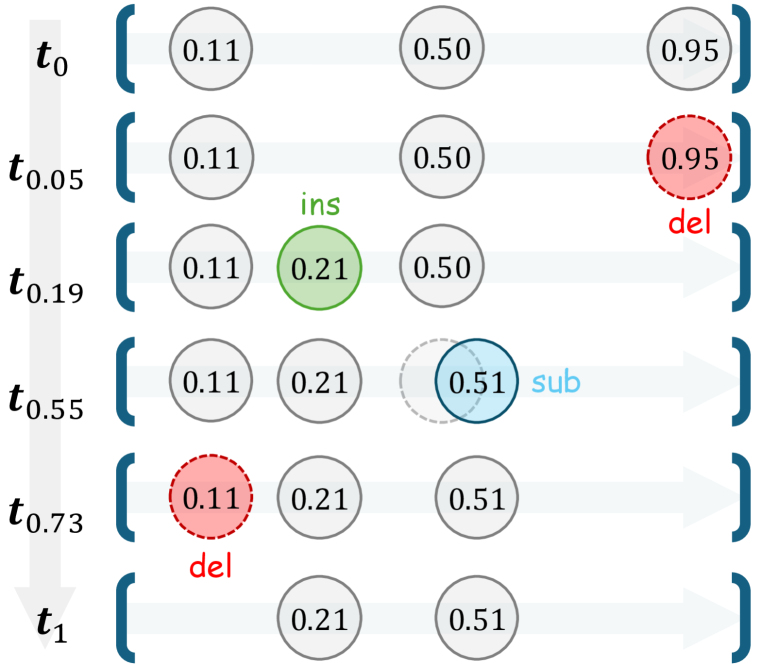
Figure 1: Edit process transporting ${\bm{t}}_{0}\sim p_{\text{noise}}({\bm{t}})$ to ${\bm{t}}_{1}\sim q_{\text{target}}({\bm{t}})$ by inserting, deleting and substituting events.

Temporal point processes (TPPs) capture the distribution over sequences of events in time, where both the continuous arrival-times and number of events are random. They are widely used in domains such as finance, healthcare, social networks, and transportation, where understanding and forecasting event dynamics and their complex interactions is crucial. Most (neural) TPPs capture the complex interactions between events autoregressively, parameterizing a conditional intensity/density of each event given its history (Daley & Vere-Jones, 2006; Shchur et al., 2021). While natural and flexible, this factorization comes with inherent limitations: sampling scales linearly with sequence length, errors can compound in multi-step generation, and conditional generation is restricted to forecasting tasks.

Beyond autoregression. Recent advances demonstrate that modeling event sequences jointly proposes a sound alternative to overcome these limitations. Inspired by diffusion, AddThin (Lüdke et al., 2023) and PSDiff (Lüdke et al., 2025) leverage the thinning and superposition properties of TPPs to construct a discrete Markov chain that learns to transform noise sequences ${\bm{t}}_{0}\sim p_{\text{noise}}({\bm{t}})$ into data sequences ${\bm{t}}_{1}\sim q_{\text{target}}({\bm{t}})$ through insertions and deletions of events. These methods highlight the promise of joint sequence modeling for TPPs by learning stochastic set interpolations and have shown state-of-the-art results, especially in forecasting.

In parallel, Havasi et al. (2025) introduced Edit Flow, a discrete flow-matching framework (Gat et al., 2024; Campbell et al., 2024; Shi et al., 2025) for variable-length sequences of tokens (e.g., language). Their approach models discrete flows in sequence space through insertions, deletions, and substitutions, formalized as a continuous-time Markov Chain (CTMC). To make the learning process tractable, they introduce an expanded auxilliary state space that aligns sequences, simultaneously reducing the complexity of marginalizing over possible transitions and enabling efficient element-wise parameterization in sequence space.

In this paper, we unify these perspectives and propose EdiTPP, an Edit Flow for TPPs that learns to transport noise sequences ${\bm{t}}_{0}\sim p_{\text{noise}}({\bm{t}})$ to data sequences ${\bm{t}}_{1}\sim q_{\text{target}}({\bm{t}})$ via atomic edit operations insertions, deletions, and substitutions (see figure 1). We define these operations specifically for TPPs, efficiently parameterize their instantaneous rates within a CTMC, propose an auxiliary alignment space for TPPs, and show that our unconditionally trained model can be flexibly applied to both unconditional and conditional tasks with adaptive complexity. Our main contributions are:

• We introduce EdiTPP, the first generative framework that models TPPs via continuous-time edit operations, unifying stochastic set interpolation methods for TPPs with Edit Flows for discrete sequences.

• We propose a tractable parameterization of insertion, deletion, and substitution rates for TPPs within the CTMC framework, effectively reducing the number of edit operations for generation.

• We demonstrate empirically that EdiTPP achieves state-of-the-art results in both unconditional and conditional tasks across diverse real-world and synthetic datasets.

2 Background

2.1 Temporal Point Processes

TPPs (Daley & Vere-Jones, 2006; 2007) are stochastic processes whose realizations are finite, ordered sets of random events in time. Let ${\bm{t}}=\{t^{(i)}\}_{i=1}^{n}$, with $t^{(i)}\in[0,T]$, denote a realization of $n$ events on a bounded time interval, which can equivalently be represented by the counting process $N(t)=\sum_{i=1}^{n}\mathbf{1}\{t^{(i)}\leq t\}$ counting the number of events up to time $t$. A TPP is uniquely characterized by its conditional intensity function (Rasmussen, 2018):

$$\lambda^{*}(t)=\lim\limits_{\Delta t\downarrow 0}\frac{\mathbb{E}[N(t+\Delta t)-N(t)\mid\mathcal{H}_{t}]}{\Delta t},$$ (1)

where $\mathcal{H}_{t}=\{t^{(i)}:t^{(i)}<t\}$ denotes the history up to time $t$. Intuitively, $\lambda^{*}(t)$ represents the instantaneous rate of events given the past. Two important properties of TPPs are superposition and thinning. Superposition, i.e., inserting one sequence into another, ${\bm{t}}={\bm{t}}_{1}\cup{\bm{t}}_{2}$, where ${\bm{t}}_{1}$ and ${\bm{t}}_{2}$ are realizations from TPPs with intensities $\lambda_{1}$ and $\lambda_{2}$, results in a sample from a TPP with intensity $\lambda=\lambda_{1}+\lambda_{2}$. Independent thinning, i.e., randomly deleting any event of a sequence from a TPP with intensity $\lambda$ with probability $p$, results in an event sequence from a TPP with intensity $(1-p)\lambda$.

The likelihood of observing an event sequence ${\bm{t}}$ given the conditional intensity/density is:

$$p({\bm{t}})=\left(\prod_{i=1}^{n}p(t^{(i)}\mid\mathcal{H}_{t^{(i)}})\right)\left(1-F(T\mid\mathcal{H}_{t})\right)=\left(\prod_{i=1}^{n}\lambda^{*}(t^{(i)})\right)\text{ exp }\left(-\int_{0}^{T}\lambda^{*}(s)\mathrm{d}s\right),$$ (2)

where $F(T\mid\mathcal{H}_{t})$ is the CDF of the conditional event density $p(t\mid\mathcal{H}_{t})$. While this autoregressive formulation of TPPs provides a natural framework for modeling event dependencies, it also poses challenges. Parameterizing the conditional intensity or density is generally nontrivial, and the inherently sequential factorization can lead to inefficient sampling, error accumulation, and limits conditional tasks to forecasting (Lüdke et al., 2023; 2025).

2.2 Modeling TPPs by set interpolation

Instead of explicitly modeling the intensity function, Lüdke et al. (2023; 2025) leverage the thinning and superposition properties of TPPs to derive diffusion-like generative models that interpolate between data event sequences ${\bm{t}}_{1}\sim q_{\text{target}}({\bm{t}})$ and noise ${\bm{t}}_{0}\sim p_{\text{noise}}({\bm{t}})$ by inserting and deleting elements. AddThin (Lüdke et al., 2023) defines the noising Markov chain recursively over a fixed number of steps with size $\Delta$ indexed by $s\in[0,1]$ as follows:

$$\lambda_{s}(t)=\underbrace{\alpha_{s}\lambda_{s-\Delta}(t)}_{\text{(i) Thin}}+\underbrace{(1-\alpha_{s})\lambda_{\mathrm{0}}(t)}_{\text{(ii) Add}},$$ (3)

where $\lambda_{1}(t)$ is the unknown target intensity of the TPP and $\alpha_{s}\in(0,1)$. Intuitively, this noising process increasingly deletes events from the data sequence, while inserting events from a noise TPP $\lambda_{\mathrm{0}}(t)$. PSDiff (Lüdke et al., 2025) further separates the adding and thinning to yield a Markov chain for the forward process, that stochastically interpolates between ${\bm{t}}_{0}$ and ${\bm{t}}_{1}$ as follows:

$$p_{s}({\bm{t}}\mid{\bm{t}}_{1},{\bm{t}}_{0})=\prod_{t\in{\bm{t}}}\begin{cases}\bar{\alpha}_{s}&\text{if }t\in{\bm{t}}_{1}\\ 1-\bar{\alpha}_{s}&\text{if }t\in{\bm{t}}_{0}\end{cases}$$ (4)

or equivalently $\lambda_{s}(t)=\bar{\alpha}_{s}\lambda_{1}(t)+(1-\bar{\alpha}_{s})\lambda_{0}(t)$, with $\bar{\alpha}_{s}$ being the product of $\alpha_{i}$’s. Eq. 4 defines an element-wise conditional path by independent insert and delete operations on TPPs, assuming ${\bm{t}}_{0}\cap{\bm{t}}_{1}=\emptyset$.

2.3 Flow matching with edit operations

Havasi et al. (2025) introduce Edit Flows, a non-autoregressive generative framework for variable-length token sequences with a fixed, discrete vocabulary (e.g., language). They propose a discrete flow that transports a noisy sequence ${\bm{x}}_{0}\sim p_{\text{noise}}({\bm{x}})$ to a data sequence ${\bm{x}}_{1}\sim q_{\text{data}}({\bm{x}})$ via elementary edit operations: insertions, deletions, and substitutions. This is formalized via the discrete flow matching framework (Gat et al., 2024; Campbell et al., 2024; Shi et al., 2025) in an augmented space, yielding a CTMC $\Pr(X_{s+h}={\bm{x}}\mid X_{s}={\bm{x}}_{s})=\delta_{{\bm{x}}_{s}}({\bm{x}})+hu_{s}^{\theta}({\bm{x}}\mid{\bm{x}}_{s})+o(h)$ with transition rates $u_{s}^{\theta}$ governed by the edit operations.

Directly defining a conditional rate $u_{s}({\bm{x}}|{\bm{x}}_{1},{\bm{x}}_{0})$ to match $u_{s}^{\theta}$ to, as in discrete flow matching, is very hard or even intractable, since all possible edits producing ${\bm{x}}$ must be considered. Thus, to train this CTMC, they rely on two major insights. First, a CTMC in a data space $\mathcal{X}$ can be learned by introducing an augmented space $\mathcal{X}\times\mathcal{Z}$ where the true dynamics are known. Second, designing the auxiliary space $\mathcal{Z}$ to follow the element wise mixture probability path $p_{s}({\bm{z}}\mid{\bm{z}}_{0},{\bm{z}}_{1})=\prod_{n}\big[(1-\kappa_{s})\delta_{z_{0}^{(i)}}(z^{(i)})+\kappa_{s}\delta_{z_{1}^{(i)}}(z^{(i)})\big]$ with kappa schedule $\kappa_{s}\in[0,1]$ (Gat et al., 2024) enables training the CTMC directly in the data space $\mathcal{X}$ of variable-length sequences.

Edit operations are encoded by mapping $({\bm{x}}_{0},{\bm{x}}_{1})$ into aligned sequences $({\bm{z}}_{0},{\bm{z}}_{1})$ in $\mathcal{Z}$, where pairs $(z_{0}^{(i)},z_{1}^{(i)})$ correspond to insertions $(\epsilon,x)$, deletions $(x,\epsilon)$, or substitutions $(x,y)$. Crucially, since the discrete flow matching dynamics in $\mathcal{Z}$ are known, they can be transferred back to $\mathcal{X}$ via $p_{s}({\bm{x}},{\bm{z}}\mid{\bm{z}}_{0},{\bm{z}}_{1})=p_{s}({\bm{z}}\mid{\bm{z}}_{0},{\bm{z}}_{1})\delta_{\operatorname{f_{rm-blanks}}({\bm{z}})}({\bm{x}})$. Then, the marginal rates $u_{s}^{{\bm{\theta}}}$ are learned in $\mathcal{X}$ by marginalizing over ${\bm{z}}$ with the Bregman divergence

$$\mathcal{L}=\operatorname*{\mathbb{E}}_{\begin{subarray}{c}({\bm{z}}_{0},{\bm{z}}_{1})\sim\pi({\bm{z}}_{0},{\bm{z}}_{1})\\ s,p_{s}({\bm{z}}_{s},{\bm{x}}_{s}\mid{\bm{z}}_{0},{\bm{z}}_{1})\end{subarray}}\bigg[\sum_{{\bm{x}}\neq{\bm{x}}_{s}}u_{s}^{{\bm{\theta}}}({\bm{x}}\mid{\bm{x}}_{s})-\sum_{z_{s}^{(i)}\neq z_{1}^{(i)}}\frac{\dot{\kappa}_{s}}{1-\kappa_{s}}\log u_{s}^{{\bm{\theta}}}\big({\bm{x}}({\bm{z}}_{s},i,z_{1}^{(i)})\mid{\bm{x}}_{s}\big)\bigg],$$ (5)

where ${\bm{x}}({\bm{z}}_{s},i,z_{1}^{(i)})=\operatorname{f_{rm-blanks}}((z_{s}^{(1)},\dots,z_{s}^{(i-1)},z_{1}^{(i)},z_{s}^{(i+1)},\dots,z_{s}^{(n)}))$.

3 Method

We introduce EdiTPP, an Edit Flow process for TPPs that directly learns the joint distribution of event times. Our process leverages the three elementary edit operations insert, substitute, and delete to define a CTMC that continuously interpolates between two event sequences ${\bm{t}}_{0}\sim p_{\text{noise}}({\bm{t}})$ and ${\bm{t}}_{1}\sim q_{\text{data}}({\bm{t}})$.

Let $\mathcal{T}=[0,T]$ denote the support of the TPP. We define the state space as $\mathcal{X}_{\mathcal{T}}\;=\;\bigcup_{n=0}^{\infty}\left\{(0,t^{(1)},\dots,t^{(n)},T)\in\mathcal{T}^{n}:0<t^{(1)}<\cdots<t^{(n)}<T\right\}$, denoting the set of all possible padded TPP sequences with finitely many events.

3.1 Edit operations

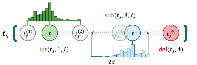
Figure 2: Our discrete edit operations transform continuous event sequences through insertions, substitutions and deletion.

Our model navigates the state space $\mathcal{X}_{\mathcal{T}}$ through a set of atomic edit operations. While Edit Flow was originally defined for discrete state spaces, we can generalize the method to continuous state spaces provided that the set of edit operations remains discrete. We achieve this by defining a finite set of edit operations on our continuous state space $\mathcal{X}_{\mathcal{T}}$ that nonetheless allow us to transition from any sequence ${\bm{t}}$ to any other ${\bm{t}}^{\prime}$ through repeated application.

Similar to Havasi et al. (2025), we design our operations to be mutually exclusive: if two sequences differ by exactly one edit, the responsible operation is uniquely determined. This simplifies the parameterization of the model and computation of the Bregman divergence in Eq. 5.

Insertion: To discretize the event insertion, we quantize the space between any two adjacent events $t^{(i)}$ and $t^{(i+1)}$ into $b_{\text{ins}}$ evenly-spaced bins. Then, we define the insertion operation relative to the $i$th event as

$$\operatorname{ins}({\bm{t}},i,j)=\Big(t^{(0)},\dots,t^{(i)},t^{(i)}+\frac{j-1+\alpha}{b_{\text{ins}}}(t^{(i+1)}-t^{(i)}),t^{(i+1)},\dots,t^{(n+1)}\Big)$$ (6)

for $i\in\{0,\dots,n\}$, $j\in[b_{\text{ins}}]$, where $\alpha\sim\mathcal{U}(0,1)$ is a dequantization factor inspired by uniform dequantization in likelihood-based generative models (Theis et al., 2016). The boundary elements $t^{(0)}=0$ and $t^{(n+1)}=T$ ensure that insertions are possible across the entire support $\mathcal{T}$. Since the bins between different $i$ are non-overlapping, insertions are mutually exclusive.

Substitution: We implement event substitutions by discretizing the continuous space around each event into $b_{\text{sub}}$ bins. In this case, the bins are free to overlap, since a substitution is always uniquely determined by the substituted event. We choose a maximum movement distance $\delta$ and define

$$\operatorname{sub}({\bm{t}},i,j)=\operatorname{sort}\Big(\{t^{(0)},\dots,t^{(i-1)},t^{(i+1)},\dots,t^{(n+1)}\}\cup\Big\{\tilde{t}^{(i)}\Big\}\Big)$$ (7)

for $i\in\{1,\dots,n\}$, $j\in[b_{\text{sub}}]$, where $\tilde{t}^{(i)}=\big[t^{(i)}-\delta+\frac{j-1+\alpha}{b_{\text{sub}}}2\delta\big]_{0}^{T}$ is the updated event restricted to the support $\mathcal{T}$ and, again, $\alpha\sim\mathcal{U}(0,1)$ is a uniform dequantization factor within the $j$-th bin.

Deletion: Finally, we define removing event $i\in\{1,\dots,n\}$ straightforwardly as

$$\operatorname{del}({\bm{t}},i)=(t^{(0)},\dots,t^{(i-1)},t^{(i+1)},\dots,t^{(n+1)}).$$ (8)

In combination, these operations facilitate any possible edit of an event sequence through insertions and deletions with substitutions as a shortcut for local delete-insert pairs. Note that we neither allow inserting after the last boundary event nor substituting or deleting the first or last boundary events, thus guaranteeing operations to stay in the state space $\mathcal{X}_{\mathcal{T}}$. We illustrate the edit operations in Fig. 2.

Parameterization

Generating a new event sequence in the Edit Flow framework then means to emit a continuous stream of edit operations by integrating a rate model $u_{s}^{{\bm{\theta}}}(\cdot\mid{\bm{t}})$ from $s=0$ to $s=1$. The emitted operations transform a noise sequence ${\bm{t}}_{0}$ into a data sample ${\bm{t}}_{1}$ by transitioning through a series of intermediate states ${\bm{t}}$. Given a current state ${\bm{t}}_{s}$, we parameterize the transition rates as

$$u_{s}^{{\bm{\theta}}}(\operatorname{ins}({\bm{t}}_{s},i,j)\mid{\bm{t}}_{s}) =\lambda_{s,i}^{\text{ins}}({\bm{t}}_{s})\,Q_{s,i}^{\text{ins}}(j\mid{\bm{t}}_{s}),$$ (9)

$$u_{s}^{{\bm{\theta}}}(\operatorname{sub}({\bm{t}}_{s},i,j)\mid{\bm{t}}_{s}) =\lambda_{s,i}^{\text{sub}}({\bm{t}}_{s})\,Q_{s,i}^{\text{sub}}(j\mid{\bm{t}}_{s}),$$ (10)

$$u_{s}^{{\bm{\theta}}}(\operatorname{del}({\bm{t}}_{s},i)\mid{\bm{t}}_{s}) =\lambda_{s,i}^{\text{del}}({\bm{t}}_{s}),$$ (11)

where $\lambda_{s,i}^{\text{del}},\lambda_{s,i}^{\text{ins}},\lambda_{s,i}^{\text{sub}}$ denote the total rate of each of the three basic operations at each event $t^{(i)}$. The distributions $Q_{s,i}^{\text{ins}}$ and $Q_{s,i}^{\text{sub}}$ are categorical distributions over the discretization bins $j\in[b_{\text{ins}}]$ and $j\in[b_{\text{sub}}]$, respectively. They distribute the total insertion and substitution rates between the specific options.

3.2 Auxiliary alignment space

Training our rate model $u_{s}^{{\bm{\theta}}}$ by directly matching a marginalized conditional rate $u_{s}({\bm{t}}\mid{\bm{t}}_{1},{\bm{t}}_{0})$ generating a $p_{s}({\bm{t}}\mid{\bm{t}}_{1},{\bm{t}}_{0})$, as is common in discrete flow matching (Campbell et al., 2024; Gat et al., 2024), is challenging or even intractable for Edit Flows, since it would require accounting for all possible edits that could produce ${\bm{t}}$ (Havasi et al., 2025).

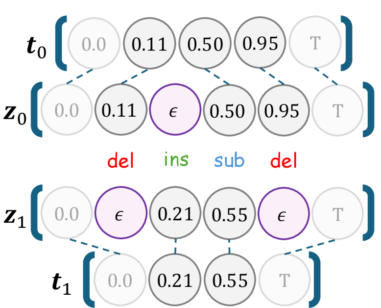
Figure 3: Illustration of the alignment space for ${\bm{t}}_{0}$ and ${\bm{t}}_{1}$.

To address this, following Havasi et al. (2025), we introduce an auxiliary alignment space for TPPs, where every possible edit operation is uniquely defined in the element wise mixture path ${\bm{z}}_{s}\sim p_{s}({\bm{z}}_{s}\mid{\bm{z}}_{0},{\bm{z}}_{1})$, making the learning problem tractable.

In language modeling, any token can appear in any position, so Havasi et al. (2025) achieve strong results even when training with a simple alignment that juxtaposes two sequences after shifting one of them by a constant number of places. In our case, for the alignments to correspond to possible edit operations, two events can only be matched, i.e., $z_{0}^{(i)}\neq\epsilon$ and $z_{1}^{(i)}\neq\epsilon$, if $|z_{0}^{(i)}-z_{1}^{(i)}|<\delta$ since otherwise the resulting $\operatorname{sub}$ operation would be invalid. Furthermore, ${\bm{z}}$s have to correspond to sequences in $\mathcal{X}_{\mathcal{T}}$, so $\operatorname{f_{rm-blanks}}({\bm{z}})$ has to be increasing, and in particular any mixing ${\bm{z}}_{s}$ between ${\bm{z}}_{0}$ and ${\bm{z}}_{1}$ needs to be valid, i.e., ${\bm{z}}_{s}\sim p_{s}({\bm{z}}_{s}\mid{\bm{z}}_{0},{\bm{z}}_{1})\Rightarrow\operatorname{f_{rm-blanks}}({\bm{z}}_{s})\in\mathcal{X}_{\mathcal{T}}$.

We find the minimum-cost alignment between the non-boundary events of ${\bm{t}}_{0}$ and ${\bm{t}}_{1}$ with the Needleman-Wunsch algorithm (Needleman & Wunsch, 1970), i.e.,

$$\operatorname{align}({\bm{t}}_{0},{\bm{t}}_{1})=\operatorname{wrap-boundaries}\!\bigg(\!\operatorname{Needleman-Wunsch}\!\Big({\bm{t}}_{0}^{(1:n)},{\bm{t}}_{1}^{(1:m)},c_{\text{ins}},c_{\text{sub}},c_{\text{del}}\Big)\!\bigg)$$ (12)

and the cost functions

$$\begin{gathered}c_{\text{sub}}(i,j)=\begin{cases}|t_{0}^{(i)}-t_{1}^{(j)}|&\text{if }|t_{0}^{(i)}-t_{1}^{(j)}|<\delta\text{ and }t_{0}^{(i-1)}<t_{1}^{(j)}<t_{0}^{(i+1)}\\ \infty&\text{otherwise}\end{cases}\\ c_{\text{ins}}(i,j)=\begin{cases}\frac{\delta}{2}&\text{if }t_{0}^{(i)}<t_{1}^{(j)}\\ \infty&\text{otherwise}\end{cases}\qquad c_{\text{del}}(i,j)=\begin{cases}\frac{\delta}{2}&\text{if }t_{0}^{(i)}>t_{1}^{(j)}\\ \infty&\text{otherwise}\end{cases}\end{gathered}$$ (13)

where $\operatorname{wrap-boundaries}$ wraps the sequences with aligned boundary events $0$ and $T$. The algorithm builds up the aligned sequences pair by pair. The operations corresponds to adding different pairs to the end of $({\bm{z}}_{0},{\bm{z}}_{1})$, i.e., insertion $\big(\epsilon,t_{1}^{(j)}\big)$, deletion $\big(t_{0}^{(i)},\epsilon\big)$ and substitution $\big(t_{0}^{(i)},t_{1}^{(j)}\big)$ (see Fig. 3).

It is trivial to see from $c_{\text{sub}}$ that the aligned sequences will never encode a $\operatorname{sub}$ operation for two events that are further than $\delta$ apart. The costs for insertions and deletions and the additional condition on $c_{\text{sub}}$ ensure that the aligned sequences are jointly sorted, i.e., for any $i<j$ we have $\max\big(z_{0}^{(i)},z_{1}^{(i)}\big)<\min\big(z_{0}^{(j)},z_{1}^{(j)}\big)$ where $\min$ and $\max$ ignore $\epsilon$ tokens. This means that any interpolated ${\bm{z}}_{s}$ will be sorted. The validity of encoded $\operatorname{ins}$ and $\operatorname{del}$ operations follows immediately.

3.3 Training

We train our model $u_{s}^{{\bm{\theta}}}(\cdot\mid{\bm{t}}_{s})$ by optimizing the Bregman divergence in Eq. 5. This amounts to sampling from a coupling $\pi({\bm{z}}_{0},{\bm{z}}_{1})$ in the aligned auxiliary space and then matching the ground-truth conditional event rates. Note that the coupling $\pi({\bm{z}}_{0},{\bm{z}}_{1})$ is implicitly defined by its sampling procedure: sample ${\bm{t}}_{0},{\bm{t}}_{1}\sim\pi({\bm{t}}_{0},{\bm{t}}_{1})$ from a coupling of the noise and data distribution, e.g., the independent coupling $\pi({\bm{t}}_{0},{\bm{t}}_{1})=p({\bm{t}}_{0})\,q({\bm{t}}_{1})$, and then align the sequences ${\bm{z}}_{0},{\bm{z}}_{1}=\operatorname{align}({\bm{t}}_{0},{\bm{t}}_{1})$. For our choice of operations, the divergence is

$$\mathcal{L}=\operatorname*{\mathbb{E}}_{\begin{subarray}{c}({\bm{z}}_{0},{\bm{z}}_{1})\sim\pi({\bm{z}}_{0},{\bm{z}}_{1})\\ s,p_{s}({\bm{z}}_{s},{\bm{t}}_{s}\mid{\bm{z}}_{0},{\bm{z}}_{1})\end{subarray}}\bigg[\sum_{\omega\in\Omega({\bm{t}}_{s})}u_{s}^{{\bm{\theta}}}(\omega\mid{\bm{t}}_{s})-\sum_{z_{s}^{(i)}\neq z_{1}^{(i)}}\frac{\dot{\kappa}_{s}}{1-\kappa_{s}}\log u_{s}^{{\bm{\theta}}}\Big(\omega\big(z_{s}^{(i)},z_{1}^{(i)}\big)\mid{\bm{t}}_{s}\Big)\bigg],$$ (14)

where $\Omega({\bm{t}}_{s})$ is the set of all edit operations applicable to ${\bm{t}}_{s}$ and $\omega\big(z_{s}^{(i)},z_{1}^{(i)}\big)$ is the edit operation encoded in the $i$-th position of the aligned sequences ${\bm{z}}_{s}$ and ${\bm{z}}_{1}$. To make it precise, we have

$$\Omega({\bm{t}}_{s})=\bigcup\begin{cases}\{\operatorname{ins}({\bm{t}}_{s},i,j)\mid i\in\{0\}\,\cup\,[n],j\in[b_{\text{ins}}]\}\\ \{\operatorname{sub}({\bm{t}}_{s},i,j)\mid i\in[n],j\in[b_{\text{sub}}]\}\\ \{\operatorname{del}({\bm{t}}_{s},i)\mid i\in[n]\}\end{cases}$$ (15)

and

$$\omega\big(z_{s}^{(i)},z_{1}^{(i)}\big)=\begin{cases}\operatorname{ins}({\bm{t}}_{s},i^{\prime},j^{\prime})&\text{if }z_{s}^{(i)}=\epsilon\text{ and }z_{1}^{(i)}\neq\epsilon,\\ \operatorname{sub}({\bm{t}}_{s},i^{\prime},j^{\prime})&\text{if }z_{s}^{(i)}\neq\epsilon\text{ and }z_{1}^{(i)}\neq\epsilon,\\ \operatorname{del}({\bm{t}}_{s},i^{\prime})&\text{if }z_{s}^{(i)}\neq\epsilon\text{ and }z_{1}^{(i)}=\epsilon.\end{cases}$$ (16)

$i^{\prime}$ is the index such that $\operatorname{f_{rm-blanks}}({\bm{z}}_{s})$ maps $z_{s}^{(i)}$ to $x_{s}^{(i^{\prime})}$ with the convention that $\epsilon$ is mapped to the same $i^{\prime}$ as the last element of ${\bm{z}}_{s}$ before $i$ that is not $\epsilon$. $j^{\prime}$ is the index of the insertion or substitution bin relative to $x_{s}^{(i^{\prime})}$ that $z_{1}^{(i)}$ falls into.

3.4 Sampling

Input: $\text{condition }{\bm{t}}_{1}^{c}=C({\bm{t}}_{1}),\text{ noise }{\bm{t}}_{0}\sim p_{\text{noise}},h=1/n_{\text{steps}}$

-0.2cm $({\bm{z}}_{0}^{c},{\bm{z}}_{1}^{c})\leftarrow\operatorname{align}(C({\bm{t}}_{0}),{\bm{t}}_{1}^{c})$

0.2cm while $s<1$ do

   

   0.1cm Euler update

    Sample edits $\omega_{s}\sim h\,u_{s}^{\theta}(\cdot\mid{\bm{t}}_{s})$

    ${\bm{t}}_{s+h}\leftarrow\text{apply }\omega_{s}\text{ to }{\bm{t}}_{s}$

   

   0.2cm Recondition

    $\tilde{{\bm{z}}}_{s+h}^{c}\sim p_{s+h}(\cdot\mid{\bm{z}}_{0}^{c},{\bm{z}}_{1}^{c})$

    ${\bm{t}}_{s+h}^{c}\leftarrow\operatorname{f_{rm-blanks}}(\tilde{{\bm{z}}}_{s+h}^{c})$

   

   0.2cm Merge

    ${\bm{t}}_{s+h}\leftarrow C^{\prime}({\bm{t}}_{s+h})\cup{\bm{t}}_{s+h}^{c}$

   

   0.2cm $s\leftarrow s+h$

   

end while

Return: forecast trajectory $C^{\prime}({\bm{t}}_{s=1})$

Algorithm 1 Conditional Sampling

Sampling from our model is done by forward simulation of the CTMC from noise ${\bm{t}}_{0}\sim p_{\text{noise}}({\bm{t}})$ up to $s=1$. We follow (Havasi et al., 2025; Gat et al., 2024) and leverage their Euler approximation, since exact simulation is intractable. Even though the rates are parameterized per element, sampling multiple edits within a time horizon can be done in parallel. At each step of length $h$, insertions at position $i$ occur with probability $h\,\lambda_{s,i}^{\text{ins}}({\bm{t}})$ and deletions or substitutions occur with probability $h(\lambda_{s,i}^{\text{del}}({\bm{t}})+\lambda_{s,i}^{\text{sub}}({\bm{t}}))$. Since they are mutually exclusive the probability of substitution vs deletion is $\lambda_{s,i}^{\text{sub}}({\bm{t}})/(\lambda_{s,i}^{\text{sub}}({\bm{t}})+\lambda_{s,i}^{\text{del}}({\bm{t}}))$. Lastly, the inserted or substituted events are drawn from the respective distributions $Q$ to update ${\bm{t}}_{s}$. For a short summary of the unconditional sampling step refer to the Euler update step depicted in algorithm Algorithm 1.

Conditional sampling. We can extend the unconditional model to conditional generation given a binary mask on time $c:\mathcal{T}\rightarrow\{0,1\}$ (e.g., for forecasting, $c(t)=t\leq t_{\text{history}}$). For a sequence ${\bm{t}}$, we define the conditioned part $C({\bm{t}})=\{t\in{\bm{t}}:c(t)=1\}$ and its complement $C^{\prime}({\bm{t}})$. Then as depicted in algorithm Algorithm 1, for conditional sampling, we can simply enforce the conditional subsequence to follow a noisy interpolation between ${\bm{t}}_{0}^{c}=C({\bm{t}}_{0})$ and ${\bm{t}}_{1}^{c}=C({\bm{t}}_{1})$, while the complement evolves freely in the sampling process.

3.5 Model Architecture

For our rate model $u_{s}^{{\bm{\theta}}}(\cdot\mid{\bm{x}}_{s})$, we adapt the Llama architecture, a transformer widely applied for variable-length sequences in language modeling (Touvron et al., 2023). We employ FlexAttention in the Llama attention blocks, which supports variable-length sequences natively without padding (Dong et al., 2024). As a first step, we convert the scalar event sequence ${\bm{x}}_{s}$ into a sequence of token embeddings by applying $\operatorname{MLP}(\operatorname{SinEmb}(x_{s}^{(i)}/T))$ to each to each event, where $\operatorname{MLP}$ refers to a small multi-layer perceptron (MLP) and $\operatorname{SinEmb}$ is a sinusoidal embedding (Vaswani et al., 2017). We convert $s$ and $|{\bm{x}}_{s}|$ into two additional tokens in an equivalent way with separate MLPs and prepend them to the embedding sequence, which we then feed to the Llama. Lastly, we apply one more MLP to map the output embedding ${\bm{h}}^{(i)}$ of each event to transition rates. In particular, we parameterize

$$\lambda_{s,i}^{\text{ins}}=\exp(\lambda_{\text{M}}\tanh({\bm{h}}_{\text{ins}}^{(i)})),\quad\lambda_{s,i}^{\text{sub}}=\exp(\lambda_{\text{M}}\tanh({\bm{h}}_{\text{sub}}^{(i)})),\quad\lambda_{s,i}^{\text{del}}=\exp(\lambda_{\text{M}}\tanh({\bm{h}}_{\text{del}}^{(i)})),$$ (17)

$${\bm{Q}}_{s,i}^{\text{ins}}=\operatorname{softmax}({\bm{h}}_{{\bm{Q}},\text{ins}}^{(i)}),\quad{\bm{Q}}_{s,i}^{\text{sub}}=\operatorname{softmax}({\bm{h}}_{{\bm{Q}},\text{sub}}^{(i)}).$$ (18)

We list the values of all relevant hyperparameters in Appendix A.

4 Experiments

We evaluate our model on seven real-world and six synthetic benchmark datasets (Omi et al., 2019; Shchur et al., 2020b; Lüdke et al., 2023; 2025). In our experiments, we compare against IFTPP (Shchur et al., 2020a), an autoregressive baseline which consistently shows state-of-the-art performance (Bosser & Taieb, 2023; Lüdke et al., 2023; Kerrigan et al., 2025). We further compare to PSDiff (Lüdke et al., 2025) and AddThin (Lüdke et al., 2023), given their strong results in both conditional and unconditional settings and their methodological similarity to our approach. All models are trained with five seeds and we select the best checkpoint based on $W_{1}$-over-$d_{\mathrm{IET}}$ against a validation set. EdiTPP, AddThin, and PSDiff are trained unconditionally but can be conditioned at inference time. We list the full results in Appendix C.

For forecasts, we compare predicted and target sequences by three metrics: $d_{\mathrm{Xiao}}$ introduced by Xiao et al. (2017), the mean relative error (MRE) of the event counts and $d_{\mathrm{IET}}$, which compares inter-event times to quantify the relation between events such as burstiness. In unconditional generation, we compare our generated sequences to the test set in terms of maximum mean discrepancy (MMD) (Shchur et al., 2020b) and their Wasserstein-1 distance with respect to their counts ($d_{l}$) and inter-event times ($d_{\mathrm{IET}}$). See Appendix B for details.

4.1 Unconditional generation

Table 1: Unconditional sampling performance. Bold is best, underlined second best. Ranking based on full results.

		H1	H2	NSP	NSR	SC	SR	PG	R/C	R/P	Tx	Tw	Y/A	Y/M
$\operatorname{MMD}$	IFTPP	$1.6$	$1.2$	$3.2$	$3.9$	$6.7$	$1.2$	$16.2$	$7.5$	$2.0$	$5.0$	$2.6$	$5.8$	$2.9$
	AddThin	$2.4$	$1.8$	$3.5$	$15.7$	$24.6$	$2.5$	$4.6$	$63.0$	$10.2$	$4.1$	$4.4$	$11.8$	$3.7$
	PSDiff	$3.3$	$1.8$	$2.0$	$5.9$	$19.8$	$2.4$	$3.2$	$6.5$	$1.0$	$3.8$	$3.4$	$4.1$	$3.4$
	EdiTPP	$1.1$	$1.2$	$1.7$	$3.5$	$7.7$	$1.0$	$1.4$	$8.2$	$2.4$	$3.1$	$1.3$	$3.7$	$4.0$
		$\times 10^{-2}$	$\times 10^{-2}$	$\times 10^{-2}$	$\times 10^{-2}$	$\times 10^{-2}$	$\times 10^{-2}$	$\times 10^{-2}$	$\times 10^{-3}$	$\times 10^{-2}$	$\times 10^{-2}$	$\times 10^{-2}$	$\times 10^{-2}$	$\times 10^{-2}$
$W_{1,d_{l}}$	IFTPP	$20.5$	$13.3$	$11.5$	$14.1$	$1.5$	$23.0$	$294.6$	$3.9$	$3.2$	$2.9$	$6.5$	$3.3$	$2.5$
	AddThin	$33.3$	$21.8$	$12.8$	$49.0$	$22.7$	$41.8$	$24.5$	$37.0$	$33.6$	$2.3$	$15.5$	$6.0$	$1.6$
	PSDiff	$26.9$	$29.6$	$5.5$	$13.3$	$10.6$	$30.3$	$16.1$	$1.3$	$2.5$	$2.8$	$6.3$	$1.5$	$1.5$
	EdiTPP	$7.6$	$7.0$	$3.1$	$1.5$	$1.3$	$6.4$	$6.2$	$1.9$	$5.7$	$2.5$	$3.4$	$1.4$	$1.7$
		$\times 10^{-3}$	$\times 10^{-3}$	$\times 10^{-3}$	$\times 10^{-3}$	$\times 10^{-3}$	$\times 10^{-3}$	$\times 10^{-3}$	$\times 10^{-2}$	$\times 10^{-2}$	$\times 10^{-2}$	$\times 10^{-3}$	$\times 10^{-2}$	$\times 10^{-2}$
$W_{1,d_{\mathrm{IET}}}$	IFTPP	$6.3$	$5.8$	$3.2$	$2.3$	$6.5$	$7.1$	$30.3$	$1.8$	$7.1$	$17.4$	$4.9$	$3.2$	$2.8$
	AddThin	$6.6$	$7.0$	$3.2$	$3.9$	$15.1$	$9.4$	$8.0$	$5.3$	$20.0$	$8.8$	$5.5$	$3.2$	$2.4$
	PSDiff	$8.6$	$9.9$	$3.0$	$5.1$	$32.6$	$12.8$	$9.0$	$1.6$	$4.3$	$11.1$	$6.7$	$2.4$	$2.3$
	EdiTPP	$5.3$	$5.5$	$3.1$	$2.2$	$6.4$	$7.0$	$7.5$	$1.4$	$6.0$	$11.1$	$4.6$	$2.5$	$2.3$
		$\times 10^{-1}$	$\times 10^{-1}$	$\times 10^{-1}$	$\times 10^{-1}$	$\times 10^{-2}$	$\times 10^{-1}$	$\times 10^{-2}$	$\times 10^{-1}$	$\times 10^{-3}$	$\times 10^{-2}$	$\times 10^{-1}$	$\times 10^{-1}$	$\times 10^{-1}$

To evaluate how well samples from each TPP model follow the data distribution, we compute distance metrics between 4000 sampled sequences and a hold-out test set. We report the unconditional sampling results in Table 1. EdiTPP achieves the best rank in unconditional sampling by strongly matching the test set distribution across all evaluation metrics, outperforming all baselines. The autoregressive baseline IFTPP shows very strong unconditional sampling capability, closely matching and on some dataset and metric combination outperforming the other non-autoregressive baselines AddThin and PSDiff.

4.2 Conditional generation (Forecasting)

Predicting the future given some history window is a fundamental TPP task. For each test sequence, we uniformly sample 50 forecasting windows $[T_{0},T],T_{0}\in[\Delta T,T-\Delta T]$, with minimal history and forecast time $\Delta T$. While, this set-up is very similar to the one proposed by Lüdke et al. (2023), there are key differences: we do not fix the forecast window and do not enforce a minimal number of forecast or history events. In fact, even an empty history encodes the information of not having observed an event and a TPP should capture the probability of not observing any event in the future.

Table 2: Forecasting accuracy up to $T$. Bold is best, underlined second best. Ranking based on full results.

		PG	R/C	R/P	Tx	Tw	Y/A	Y/M
$d_{\mathrm{Xiao}}$	IFTPP	$6.0$	$3.9$	$6.3$	$4.7$	$2.6$	$1.8$	$3.4$
	AddThin	$2.5$	$8.8$	$7.3$	$4.0$	$2.8$	$1.5$	$2.9$
	PSDiff	$2.4$	$3.2$	$4.8$	$4.4$	$2.6$	$1.5$	$3.0$
	EdiTPP	$2.5$	$3.4$	$4.9$	$4.5$	$2.7$	$1.5$	$3.0$
			$\times 10^{1}$	$\times 10^{1}$
MRE	IFTPP	$38.9$	$7.5$	$3.5$	$3.2$	$2.1$	$3.7$	$3.9$
	AddThin	$3.7$	$14.8$	$4.6$	$3.0$	$3.0$	$3.5$	$3.7$
	PSDiff	$3.4$	$3.3$	$3.0$	$11.4$	$2.4$	$3.5$	$9.2$
	EdiTPP	$3.5$	$3.6$	$2.8$	$12.3$	$2.3$	$3.5$	$9.0$
		$\times 10^{-1}$		$\times 10^{-1}$	$\times 10^{-1}$		$\times 10^{-1}$	$\times 10^{-1}$
$d_{\mathrm{IET}}$	IFTPP	$4.7$	$6.8$	$14.7$	$1.4$	$2.2$	$5.9$	$3.9$
	AddThin	$4.0$	$6.9$	$10.3$	$1.2$	$1.5$	$4.9$	$2.6$
	PSDiff	$4.1$	$6.2$	$9.5$	$1.1$	$1.5$	$4.9$	$2.6$
	EdiTPP	$4.0$	$6.8$	$10.1$	$1.1$	$1.4$	$5.0$	$2.7$
		$\times 10^{-1}$	$\times 10^{-1}$	$\times 10^{-3}$	$\times 10^{-1}$		$\times 10^{-1}$	$\times 10^{-1}$

We report the forecasting results in Table 2. EdiTPP shows very strong forecasting capabilities closely matching or surpassing the baselines across most dataset and metric combinations. Even though IFTPP is explicitly trained to auto-regressively predict the next event given its history, it shows overall worse forecasting capabilities compared to the unconditionally trained EdiTPP, AddThin and PSDiff. This again, underlines previous findings (Lüdke et al., 2023), that autoregressive TPPs can suffer from error accumulation in forecasting. Similar to the unconditional setting, PSDiff (transformer) outperforms AddThin (convolution with circular padding), which showcases the improved posterior and modeling of long-range interactions.

4.3 Edit efficiency

Table 3: Average number of edit operations in unconditional sampling across datasets.

	Ins	Del	Sub	Total
PSDiff	171.47	61.22	–	232.68
EdiTPP	132.88	31.43	28.97	193.29

The $\operatorname{sub}$ operation allows our model to modify sequences in a more targeted way when compared to PSDiff or AddThin, which have to rely on just inserts and deletes. Note that one $\operatorname{sub}$ operation can replace an insert-delete pair. Table 3 shows this results in EdiTPP using fewer edit operations than PSDiff on average even if one would count substitutions twice, as an insert and a delete. This is further amplified by the fact, that unlike EdiTPP, PSDiff and AddThin only indirectly parameterizes the transition edit rates by predicting ${\bm{t}}_{1}$ by insertion and deletion at every sampling step.

Figure 4: Changing the number of steps $k$ allows trading off compute and sample quality in terms of $d_{l}$, $d_{W_{2}}$ and $d_{\mathrm{IET}}$ at inference time.

Table 4: Sample run-time (ms) on a H100 GPU.

	R/P	R/C
AddThin	18,075.62	17,689.36
PSDiff	7,776.35	3,913.78
EdiTPP	4,120.38	1,505.68

In Table 4, we compare their actual sampling runtime for a batch size of 1024 on the two dataset with the longest sequences. Our implementation beats the reference implementations of AddThin and PSDiff by a large margin. Note, that for a fair comparison, we fixed the number of sampling steps to 100 in all previous evaluations. As a continuous-time model, EdiTPP can further trade off compute against sample quality at inference time without retraining, in contrast to discrete-time models like AddThin and PSDiff. Fig. 4 shows that sample quality improves as we increase the number of sampling steps and therefore reduce the discretization step size of the CTMC dynamics. At the same time, the figure also shows rapidly diminishing quality improvements, highlighting potential for substantial speedups with only minor quality loss.

5 Related work

The statistical modeling of TPPs has a long history (Daley & Vere-Jones, 2007; Hawkes, 1971). Classical approaches such as the Hawkes process define parametric conditional intensities, but their limited flexibility has motivated the development of neurally parameterized TPPs:

Autoregressive Neural TPP: Most neural TPPs adopt an autoregressive formulation, modeling the distribution of each event conditional on its history. These models consist of two components: a history encoder and an event decoder. Encoders are typically implemented using recurrent neural networks (Du et al., 2016; Shchur et al., 2020a) or attention mechanisms (Zhang et al., 2020a; Zuo et al., 2020; Mei et al., 2022), with attention-based models providing longer-range context at the cost of higher complexity (Shchur et al., 2021). Further, some propose to encode the history of a TPP in a continuous latent stochastic processes (Chen et al., 2020; Enguehard et al., 2020; Jia & Benson, 2019; Hasan et al., 2023). For the decoder, a wide variety of parametrizations have been explored. Conditional intensities or related measures (e.g., hazard function or conditional density), can be modeled, parametrically (Mei & Eisner, 2017; Zuo et al., 2020; Zhang et al., 2020a), via neural networks (Omi et al., 2019), mixtures of kernels (Okawa et al., 2019; Soen et al., 2021; Zhang et al., 2020b) and mixture distributions (Shchur et al., 2020a). Generative approaches further enhance flexibility: normalizing flow-based (Shchur et al., 2020b), GAN-based (Xiao et al., 2017), VAE-based (Li et al., 2018), and diffusion-based decoders (Lin et al., 2022; Yuan et al., 2023) have all been proposed. While expressive, autoregressive TPPs are inherently sequential, which makes sampling scale at least linearly with sequence length, can lead to error accumulation in multi-step forecasting and limit conditional generation to forecasting.

Non-autoregressive Neural TPPs: Similar to our method, these approaches model event sequences through a latent variable process that refines the entire sequence jointly. Diffusion-inspired (Lüdke et al., 2023; 2025) and flow-based generative models (Kerrigan et al., 2025) have recently emerged as promising alternatives to auto-regressive TPP models by directly modelling the joint distribution over event sequences.

6 Conclusion

We have presented EdiTPP, an Edit Flow for TPPs that generalises diffusion-based set interpolation methods (Lüdke et al., 2023; 2025) with a continuous-time flow model introducing substitution as an additional edit operation. By parameterizing insertions, deletions, and substitutions within a CTMC, our approach enables efficient and flexible sequence modeling for TPPs. Empirical results demonstrate that EdiTPP matches state-of-the-art performance in both unconditional and conditional generation tasks across synthetic and real-world datasets, while reducing the number of edit operations.

appendix.0appendix.0AppendixAppendixappendix.0

Appendix A Model Parameters

Table 5: Hyperparameters of our $u_{s}^{{\bm{\theta}}}(\cdot\mid{\bm{x}}_{s})$ model shared across all datasets.

Parameter	Value
Number of $\operatorname{ins}$ bins $b_{\text{ins}}$	64
Number of $\operatorname{sub}$ bins $b_{\text{sub}}$	64
Maximum $\operatorname{sub}$ distance $\delta$	$\nicefrac{{T}}{{100}}$
Maximum log-rate $\lambda_{\text{M}}$	32
$\kappa(s)$	$1-{\cos\big(\frac{\pi}{2}s\big)}^{2}$
Llama architecture:
Hidden size $H$	64
Layers	2
Attention heads	4
Optimizer	Adam
Sample steps	100

All MLPs have input and output sizes of $H$, except for the final MLP whose output size is determined by the number of $\lambda$ and $Q$ parameters of the rate. The MLPs have a single hidden layer of size $4H$. The sinusoidal embeddings map a scalar $s\in[0,1]$ to a vector of length $H$. In contrast to Havasi et al. (2025), we choose a cosine $\kappa$ schedule $\kappa(s)=1-{\cos\big(\frac{\pi}{2}s\big)}^{2}$ as proposed by Nichol & Dhariwal (2021) for diffusion models as it improved results slightly compared $\kappa(s)=s^{3}$.

For evaluation, we use an exponential moving average (EMA) of the model weights. We also use low-discrepancy sampling of $s$ in Eq. 14 during training to smooth the loss and thus training signal (Kingma et al., 2023; Lienen et al., 2025).

We train all models for $20\,000$ steps and select the best checkpoint by its $W_{1}$-over-$d_{\mathrm{IET}}$, which we evaluate on a validation set every $1000$ steps.

Appendix B Metrics

A standard way in generative modeling to compare generated and real data is the Wasserstein distance (Heusel et al., 2017). It is the minimum average distance between elements of the two datasets under the optimal (partial) assignment between them,

$$W_{p}(\mathcal{X},\mathcal{X}^{\prime})={\Big(\min\nolimits_{\gamma\in\Gamma(\mathcal{X},\mathcal{X}^{\prime})}\operatorname*{\mathbb{E}}\nolimits_{({\bm{x}},{\bm{x}}^{\prime})\sim\gamma}\,\big[{d({\bm{x}},{\bm{x}}^{\prime})}^{p}\big]\Big)}^{\nicefrac{{1}}{{p}}}$$ (19)

where $d$ is a distance that compares elements from the two sets. In the case of sequences of unequal length, one can choose $d$ itself as a nested Wasserstein distance (Lienen et al., 2024). Xiao et al. (2017) were the first to design such a distance between TPPs. They exploit a special case of $W_{1}$ for sorted sequences of equal length and assign the remaining events of the longer sequence to pseudo-events at $T$ to define

$$d_{\mathrm{Xiao}}({\bm{x}},{\bm{x}}^{\prime})=\sum\nolimits_{i=1}^{|{\bm{x}}|}|t^{(i)}-t^{\prime(i)}|+\sum\nolimits_{i=|{\bm{x}}|+1}^{|{\bm{x}}^{\prime}|}|T-t^{\prime(i)}|$$ (20)

where ${\bm{x}}^{\prime}$ is assumed to be the longer sequence. $d_{\mathrm{Xiao}}$ captures a difference in both location and number of events between two sequences through its two terms.

(Shchur et al., 2020b) propose to compute the MMD between sets based on a Gaussian kernel and $d_{\mathrm{Xiao}}$. In addition, we evaluate the event count distributions via a Wasserstein-1 distance with respect to a difference in event counts $W_{1,d_{l}}$ where $d_{l}({\bm{x}},{\bm{x}}^{\prime})=\big||{\bm{x}}|-|{\bm{x}}^{\prime}|\big|$. Finally, we the distributions of inter-event times between our generated sequences and real sequences in $W_{1,d_{\mathrm{IET}}}$, i.e., a Wasserstein-1 distance of $d_{\mathrm{IET}}$. $d_{\mathrm{IET}}$ is itself the $W_{2}$ distance between inter-event times of two sequences and quantifies how adjacent events relate to each other to capture more complex patterns.

Appendix C Detailed Results

Table 6: Forecasting accuracy up to $T$ measured by $d_{\mathrm{IET}}$.

	EdiTPP	PSDiff	AddThin	IFTPP
PUBG	$0.400(2)$	$0.413(9)$	$0.403(10)$	$0.473(19)$
Reddit Comments	$0.684(5)$	$0.625(12)$	$0.693(12)$	$0.684(12)$
Reddit Posts	$0.010()$	$0.009()$	$0.010(1)$	$0.015(3)$
Taxi	$0.113(3)$	$0.113(1)$	$0.116(1)$	$0.145(9)$
Twitter	$1.441(20)$	$1.487(12)$	$1.493(33)$	$2.187(29)$
Yelp Airport	$0.497(9)$	$0.492(5)$	$0.493(13)$	$0.587(19)$
Yelp Mississauga	$0.272(3)$	$0.262(3)$	$0.260(3)$	$0.388(24)$

Table 7: Forecasting accuracy up to $T$ measured by mean relative error of event counts.

	EdiTPP	PSDiff	AddThin	IFTPP
PUBG	$0.349(1)$	$0.339(8)$	$0.367(5)$	$3.892(35)$
Reddit Comments	$3.594(118)$	$3.260(268)$	$14.777(3226)$	$7.515(2112)$
Reddit Posts	$0.281(1)$	$0.296(6)$	$0.457(65)$	$0.352(22)$
Taxi	$1.234(36)$	$1.140(43)$	$0.301(14)$	$0.321(18)$
Twitter	$2.327(42)$	$2.435(106)$	$2.984(246)$	$2.060(27)$
Yelp Airport	$0.350(7)$	$0.346(4)$	$0.347(14)$	$0.366(9)$
Yelp Mississauga	$0.902(27)$	$0.920(33)$	$0.374(12)$	$0.392(12)$

Table 8: Forecasting accuracy up to $T$ measured by $d_{\mathrm{Xiao}}$.

	EdiTPP	PSDiff	AddThin	IFTPP
PUBG	$2.478(7)$	$2.400(7)$	$2.466(24)$	$5.954(195)$
Reddit Comments	$34.135(382)$	$32.467(534)$	$87.666(20\,184)$	$39.010(7508)$
Reddit Posts	$48.776(355)$	$47.829(1050)$	$72.754(12\,134)$	$63.256(9695)$
Taxi	$4.464(88)$	$4.444(76)$	$4.032(129)$	$4.744(125)$
Twitter	$2.669(22)$	$2.635(78)$	$2.802(132)$	$2.557(55)$
Yelp Airport	$1.524(13)$	$1.512(16)$	$1.548(26)$	$1.795(15)$
Yelp Mississauga	$3.027(46)$	$3.005(46)$	$2.895(39)$	$3.430(47)$

Table 9: Sample quality as measured by $\operatorname{MMD}$.

	EdiTPP	PSDiff	AddThin	IFTPP
Hawkes-1	$0.011(2)$	$0.033(9)$	$0.024(9)$	$0.016(2)$
Hawkes-2	$0.012(1)$	$0.018(6)$	$0.018(6)$	$0.012(1)$
Nonstationary Poisson	$0.017(3)$	$0.020(5)$	$0.035(11)$	$0.032(8)$
Nonstationary Renewal	$0.035(1)$	$0.059(6)$	$0.157(84)$	$0.039(7)$
PUBG	$0.014(1)$	$0.032(12)$	$0.046(25)$	$0.162(10)$
Reddit Comments	$0.008(1)$	$0.006(2)$	$0.063(12)$	$0.007(3)$
Reddit Posts	$0.024(1)$	$0.010(2)$	$0.102(4)$	$0.020(7)$
Self-Correcting	$0.077(4)$	$0.198(2)$	$0.246(18)$	$0.067(11)$
Stationary Renewal	$0.010(2)$	$0.024(5)$	$0.025(13)$	$0.012(2)$
Taxi	$0.031(2)$	$0.038(5)$	$0.041(4)$	$0.050(3)$
Twitter	$0.013(2)$	$0.034(7)$	$0.044(12)$	$0.026(5)$
Yelp Airport	$0.037(2)$	$0.041(4)$	$0.118(36)$	$0.058(2)$
Yelp Mississauga	$0.040(3)$	$0.034(7)$	$0.037(6)$	$0.029(2)$

Table 10: Sample quality as measured by $W_{1}$-over-$d_{\mathrm{IET}}$.

	EdiTPP	PSDiff	AddThin	IFTPP
Hawkes-1	$0.526(20)$	$0.865(35)$	$0.655(81)$	$0.628(30)$
Hawkes-2	$0.546(5)$	$0.991(38)$	$0.703(49)$	$0.582(9)$
Nonstationary Poisson	$0.306(5)$	$0.303(7)$	$0.318(15)$	$0.317(6)$
Nonstationary Renewal	$0.224(6)$	$0.511(16)$	$0.393(64)$	$0.229(27)$
PUBG	$0.075()$	$0.090(1)$	$0.080(3)$	$0.303(39)$
Reddit Comments	$0.144(3)$	$0.157(6)$	$0.532(14)$	$0.176(8)$
Reddit Posts	$0.006()$	$0.004()$	$0.020(1)$	$0.007(1)$
Self-Correcting	$0.064()$	$0.326(3)$	$0.151(5)$	$0.065(1)$
Stationary Renewal	$0.697(18)$	$1.281(49)$	$0.941(145)$	$0.714(28)$
Taxi	$0.111(1)$	$0.111(1)$	$0.088(3)$	$0.174(15)$
Twitter	$0.460(4)$	$0.672(7)$	$0.545(24)$	$0.492(23)$
Yelp Airport	$0.246(2)$	$0.244(4)$	$0.316(46)$	$0.318(17)$
Yelp Mississauga	$0.226(3)$	$0.225(3)$	$0.236(4)$	$0.276(17)$

Table 11: Sample quality as measured by $W_{1}$-over-$d_{l}$.

	EdiTPP	PSDiff	AddThin	IFTPP
Hawkes-1	$0.008(1)$	$0.027(8)$	$0.033(15)$	$0.020(4)$
Hawkes-2	$0.007(1)$	$0.030(9)$	$0.022(14)$	$0.013(3)$
Nonstationary Poisson	$0.003(1)$	$0.006(1)$	$0.013(5)$	$0.012(3)$
Nonstationary Renewal	$0.001()$	$0.013(1)$	$0.049(22)$	$0.014(11)$
PUBG	$0.006()$	$0.016(8)$	$0.024(14)$	$0.295(7)$
Reddit Comments	$0.019(2)$	$0.013(3)$	$0.370(81)$	$0.039(23)$
Reddit Posts	$0.057(3)$	$0.025(3)$	$0.336(45)$	$0.032(11)$
Self-Correcting	$0.001()$	$0.011(1)$	$0.023(2)$	$0.001(1)$
Stationary Renewal	$0.006(2)$	$0.030(19)$	$0.042(22)$	$0.023(5)$
Taxi	$0.025(2)$	$0.028(4)$	$0.023(6)$	$0.029(3)$
Twitter	$0.003(1)$	$0.006(3)$	$0.015(8)$	$0.007(2)$
Yelp Airport	$0.014(2)$	$0.015(4)$	$0.060(21)$	$0.033(3)$
Yelp Mississauga	$0.017(3)$	$0.015(2)$	$0.016(3)$	$0.025(6)$

Table 12: Average number of edit operations during unconditional sampling.

	EdiTPP			PSDiff
	Ins	Del	Sub	Ins	Del
Hawkes-1	56.78	61.81	38.09	90.98	104.06
Hawkes-2	64.04	69.62	30.74	91.26	104.60
Nonstationary Poisson	49.51	49.26	50.56	100.22	99.66
Nonstationary Renewal	42.36	44.41	55.82	96.37	98.48
Self-Correcting	34.61	34.46	66.15	99.40	99.27
Stationary Renewal	71.57	62.86	38.11	106.08	103.38
PUBG	56.40	19.88	19.93	76.43	41.06
Reddit Comments	237.27	8.75	15.15	275.13	24.51
Reddit Posts	956.10	0.10	23.73	1091.55	24.41
Taxi	81.71	7.13	16.37	98.53	23.19
Twitter	11.53	21.48	2.94	15.27	24.05
Yelp Airport	21.80	15.61	8.40	30.84	24.53
Yelp Mississauga	43.79	13.28	10.60	56.99	24.64
Mean	132.88	31.43	28.97	171.47	61.22
Total	193.29			232.68

References

- Bosser & Taieb (2023) Tanguy Bosser and Souhaib Ben Taieb. On the predictive accuracy of neural temporal point process models for continuous-time event data. Transactions on Machine Learning Research, 2023. ISSN 2835-8856. URL https://openreview.net/forum?id=3OSISBQPrM. Survey Certification.
- Campbell et al. (2024) Andrew Campbell, Jason Yim, Regina Barzilay, Tom Rainforth, and Tommi Jaakkola. Generative flows on discrete state-spaces: Enabling multimodal flows with applications to protein co-design, 2024. URL https://arxiv.org/abs/2402.04997.
- Chen et al. (2020) Ricky TQ Chen, Brandon Amos, and Maximilian Nickel. Neural spatio-temporal point processes. arXiv preprint arXiv:2011.04583, 2020.
- Daley & Vere-Jones (2007) Daryl J Daley and David Vere-Jones. An introduction to the theory of point processes: volume II: general theory and structure. Springer Science & Business Media, 2007.
- Daley & Vere-Jones (2006) D.J. Daley and D. Vere-Jones. An Introduction to the Theory of Point Processes: Volume I: Elementary Theory and Methods. Probability and Its Applications. Springer New York, 2006.
- Dong et al. (2024) Juechu Dong, Boyuan Feng, Driss Guessous, Yanbo Liang, and Horace He. Flex Attention: A Programming Model for Generating Optimized Attention Kernels, December 2024.
- Du et al. (2016) Nan Du, Hanjun Dai, Rakshit Trivedi, Utkarsh Upadhyay, Manuel Gomez-Rodriguez, and Le Song. Recurrent marked temporal point processes: Embedding event history to vector. In Proceedings of the 22nd ACM SIGKDD international conference on knowledge discovery and data mining, pp. 1555–1564, 2016.
- Enguehard et al. (2020) Joseph Enguehard, Dan Busbridge, Adam Bozson, Claire Woodcock, and Nils Hammerla. Neural temporal point processes for modelling electronic health records. In Machine Learning for Health, pp. 85–113. PMLR, 2020.
- Gat et al. (2024) Itai Gat, Tal Remez, Neta Shaul, Felix Kreuk, Ricky T. Q. Chen, Gabriel Synnaeve, Yossi Adi, and Yaron Lipman. Discrete flow matching, 2024. URL https://arxiv.org/abs/2407.15595.
- Hasan et al. (2023) Ali Hasan, Yu Chen, Yuting Ng, Mohamed Abdelghani, Anderson Schneider, and Vahid Tarokh. Inference and sampling of point processes from diffusion excursions. In The 39th Conference on Uncertainty in Artificial Intelligence, 2023.
- Havasi et al. (2025) Marton Havasi, Brian Karrer, Itai Gat, and Ricky T. Q. Chen. Edit flows: Flow matching with edit operations, 2025. URL https://arxiv.org/abs/2506.09018.
- Hawkes (1971) Alan G Hawkes. Spectra of some self-exciting and mutually exciting point processes. Biometrika, 58(1):83–90, 1971.
- Heusel et al. (2017) Martin Heusel, Hubert Ramsauer, Thomas Unterthiner, Bernhard Nessler, and Sepp Hochreiter. GANs Trained by a Two Time-Scale Update Rule Converge to a Local Nash Equilibrium. In Neural Information Processing Systems, 2017.
- Jia & Benson (2019) Junteng Jia and Austin R Benson. Neural jump stochastic differential equations. Advances in Neural Information Processing Systems, 32, 2019.
- Kerrigan et al. (2025) Gavin Kerrigan, Kai Nelson, and Padhraic Smyth. Eventflow: Forecasting temporal point processes with flow matching, 2025. URL https://arxiv.org/abs/2410.07430.
- Kingma et al. (2023) Diederik P. Kingma, Tim Salimans, Ben Poole, and Jonathan Ho. Variational Diffusion Models, April 2023.
- Li et al. (2018) Shuang Li, Shuai Xiao, Shixiang Zhu, Nan Du, Yao Xie, and Le Song. Learning temporal point processes via reinforcement learning. Advances in neural information processing systems, 31, 2018.
- Lienen et al. (2024) Marten Lienen, David Lüdke, Jan Hansen-Palmus, and Stephan Günnemann. From Zero to Turbulence: Generative Modeling for 3D Flow Simulation. In International Conference on Learning Representations, 2024.
- Lienen et al. (2025) Marten Lienen, Marcel Kollovieh, and Stephan Günnemann. Generative Modeling with Bayesian Sample Inference, 2025.
- Lin et al. (2022) Haitao Lin, Lirong Wu, Guojiang Zhao, Liu Pai, and Stan Z Li. Exploring generative neural temporal point process. Transactions on Machine Learning Research, 2022.
- Lüdke et al. (2023) David Lüdke, Marin Biloš, Oleksandr Shchur, Marten Lienen, and Stephan Günnemann. Add and thin: Diffusion for temporal point processes. In Thirty-seventh Conference on Neural Information Processing Systems, 2023. URL https://openreview.net/forum?id=tn9Dldam9L.
- Lüdke et al. (2025) David Lüdke, Enric Rabasseda Raventós, Marcel Kollovieh, and Stephan Günnemann. Unlocking point processes through point set diffusion. In The Thirteenth International Conference on Learning Representations, 2025. URL https://openreview.net/forum?id=4anfpHj0wf.
- Mei & Eisner (2017) Hongyuan Mei and Jason M Eisner. The neural hawkes process: A neurally self-modulating multivariate point process. In Neural Information Processing Systems (NeurIPS), 2017.
- Mei et al. (2022) Hongyuan Mei, Chenghao Yang, and Jason Eisner. Transformer embeddings of irregularly spaced events and their participants. In International Conference on Learning Representations, 2022. URL https://openreview.net/forum?id=Rty5g9imm7H.
- Needleman & Wunsch (1970) Saul B. Needleman and Christian D. Wunsch. A general method applicable to the search for similarities in the amino acid sequence of two proteins. Journal of Molecular Biology, 48(3):443–453, March 1970. ISSN 0022-2836. doi: 10.1016/0022-2836(70)90057-4.
- Nichol & Dhariwal (2021) Alex Nichol and Prafulla Dhariwal. Improved Denoising Diffusion Probabilistic Models. In International Conference on Machine Learning, 2021. doi: 10.48550/arXiv.2102.09672.
- Okawa et al. (2019) Maya Okawa, Tomoharu Iwata, Takeshi Kurashima, Yusuke Tanaka, Hiroyuki Toda, and Naonori Ueda. Deep mixture point processes: Spatio-temporal event prediction with rich contextual information. In Proceedings of the 25th ACM SIGKDD International Conference on Knowledge Discovery & Data Mining, pp. 373–383, 2019.
- Omi et al. (2019) Takahiro Omi, Kazuyuki Aihara, et al. Fully neural network based model for general temporal point processes. Advances in neural information processing systems, 32, 2019.
- Rasmussen (2018) Jakob Gulddahl Rasmussen. Lecture notes: Temporal point processes and the conditional intensity function, 2018. URL https://arxiv.org/abs/1806.00221.
- Shchur et al. (2020a) Oleksandr Shchur, Marin Biloš, and Stephan Günnemann. Intensity-free learning of temporal point processes. In International Conference on Learning Representations (ICLR), 2020a.
- Shchur et al. (2020b) Oleksandr Shchur, Nicholas Gao, Marin Biloš, and Stephan Günnemann. Fast and flexible temporal point processes with triangular maps. In Advances in Neural Information Processing Systems (NeurIPS), 2020b.
- Shchur et al. (2021) Oleksandr Shchur, Ali Caner Türkmen, Tim Januschowski, and Stephan Günnemann. Neural temporal point processes: A review. arXiv preprint arXiv:2104.03528, 2021.
- Shi et al. (2025) Jiaxin Shi, Kehang Han, Zhe Wang, Arnaud Doucet, and Michalis K. Titsias. Simplified and generalized masked diffusion for discrete data, 2025. URL https://arxiv.org/abs/2406.04329.
- Soen et al. (2021) Alexander Soen, Alexander Mathews, Daniel Grixti-Cheng, and Lexing Xie. Unipoint: Universally approximating point processes intensities. In Proceedings of the AAAI Conference on Artificial Intelligence, volume 35, pp. 9685–9694, 2021.
- Theis et al. (2016) Lucas Theis, Aäron van den Oord, and Matthias Bethge. A note on the evaluation of generative models. In International Conference on Learning Representations. arXiv, 2016. doi: 10.48550/arXiv.1511.01844.
- Touvron et al. (2023) Hugo Touvron, Thibaut Lavril, Gautier Izacard, Xavier Martinet, Marie-Anne Lachaux, Timothée Lacroix, Baptiste Rozière, Naman Goyal, Eric Hambro, Faisal Azhar, Aurelien Rodriguez, Armand Joulin, Edouard Grave, and Guillaume Lample. LLaMA: Open and Efficient Foundation Language Models, February 2023.
- Vaswani et al. (2017) Ashish Vaswani, Noam Shazeer, Niki Parmar, Jakob Uszkoreit, Llion Jones, Aidan N. Gomez, Lukasz Kaiser, and Illia Polosukhin. Attention Is All You Need. In Neural Information Processing Systems, 2017.
- Xiao et al. (2017) Shuai Xiao, Mehrdad Farajtabar, Xiaojing Ye, Junchi Yan, Le Song, and Hongyuan Zha. Wasserstein learning of deep generative point process models. Advances in neural information processing systems, 30, 2017.
- Yuan et al. (2023) Yuan Yuan, Jingtao Ding, Chenyang Shao, Depeng Jin, and Yong Li. Spatio-temporal Diffusion Point Processes. In Proceedings of the 29th ACM SIGKDD Conference on Knowledge Discovery and Data Mining, pp. 3173–3184, New York, NY, USA, 2023. Association for Computing Machinery.
- Zhang et al. (2020a) Qiang Zhang, Aldo Lipani, Omer Kirnap, and Emine Yilmaz. Self-attentive hawkes process. In International conference on machine learning, pp. 11183–11193. PMLR, 2020a.
- Zhang et al. (2020b) Wei Zhang, Thomas Panum, Somesh Jha, Prasad Chalasani, and David Page. Cause: Learning granger causality from event sequences using attribution methods. In International Conference on Machine Learning, pp. 11235–11245. PMLR, 2020b.
- Zuo et al. (2020) Simiao Zuo, Haoming Jiang, Zichong Li, Tuo Zhao, and Hongyuan Zha. Transformer hawkes process. arXiv preprint arXiv:2002.09291, 2020.
appendix.0appendix.0\EdefEscapeHexAppendixAppendix\hyper@anchorstartappendix.0\hyper@anchorend