BLISS: A Lightweight Bilevel Influence Scoring Method for Data Selection in Language Model Pretraining

Abstract

Effective data selection is essential for pretraining large language models (LLMs), enhancing efficiency and improving generalization to downstream tasks. However, existing approaches often require leveraging external pretrained models, making it difficult to disentangle the effects of data selection from those of the external pretrained models. In addition, they often overlook the long-term impact of selected data if the model is trained to convergence, primarily due to the prohibitive cost of full-scale LLM pretraining. In this paper, we introduce BLISS (BileveL Influence Scoring method for data Selection): a lightweight data selection method that operates entirely from scratch, without relying on any external pretrained oracle models, while explicitly accounting for the long-term impact of selected data. BLISS leverages a small proxy model as a surrogate for the LLM and employs a score model to estimate the long-term influence of training samples if the proxy model is trained to convergence. We formulate data selection as a bilevel optimization problem, where the upper-level objective optimizes the score model to assign importance weights to training samples, ensuring that minimizing the lower-level objective (i.e., training the proxy model over the weighted training loss until convergence) leads to best validation performance. Once optimized, the trained score model predicts influence scores for the dataset, enabling efficient selection of high-quality samples for LLM pretraining. We validate BLISS by pretraining 410M/1B/2.8B Pythia and LLaMA-0.5B models on selected subsets of the C4 dataset. Notably, under the 1B model setting, BLISS achieves $1.7\times$ speedup in reaching the same performance as the state-of-the-art method, demonstrating superior performance across multiple downstream tasks.

1 Introduction

The successful large-scale language model pretraining crucially relies on the careful choice of pretraining data (Brown et al., 2020; Raffel et al., 2020; Du et al., 2022; Elazar et al., 2023). Recent studies have shown that effective data selection (a.k.a., data curation) methods can enhance pretraining efficiency (Xie et al., 2023a) and improve generalization (Engstrom et al., 2024; Wettig et al., 2024). There are various types of data selection approaches for language model pretraining, including language filtering (Laurençon et al., 2022; Wenzek et al., 2019), data deduplication (Lee et al., 2021; Abbas et al., 2023), heuristic approaches (Rae et al., 2021; Penedo et al., 2023), data quality data filtering (Brown et al., 2020; Gao et al., 2020; Chowdhery et al., 2023; Xie et al., 2023b; Wettig et al., 2024), data mixing (Xie et al., 2023a; Albalak et al., 2023; Xia et al., 2023), and data influence function based methods (Park et al., 2023; Engstrom et al., 2024; Yu et al., 2024). Despite the rich literature of data selection methods in large language model (LLM) pretraining (e.g., a survey paper in Albalak et al. (2024)), it is still unclear what properties are needed for the training data curation to guarantee good performance: it remains an important real-world challenge (Li et al., 2024).

Existing approaches of data selection methods suffer from two major limitations. First, they often require leveraging pretrained models (Brown et al., 2020; Xie et al., 2023b; Wettig et al., 2024) for data-quality filtering, making it difficult to separate the effects of data selection from those of the external pretrained models. For example, the QuRating method (Wettig et al., 2024) assigns quality ratings to training samples based on responses from a pretrained LLM (e.g., GPT-3.5) before training a QuRater model. This reliance raises uncertainty about the role of the external LLM in the training process and whether its feedback is truly optimal. Moreover, the cost of invoking these external pretrained models is prohibitively expensive during data selection process for large-scale pretraining. Second, they typically do not consider the long-term impact of selected data if the model is trained to convergence. For example, the data influence function based approach (Yu et al., 2024) evaluates the impact of individual training samples based on a single training step with the current model, which does not capture the cumulative effects of data selection over the course of full model training.

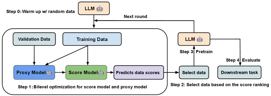
Figure 1: The pipeline of data selection and pretraining procedure. There are four main steps in one round training, 1) Warm up LLM using randomly selected training data (e.g. 10k step); 2) Bilevel optimization for score and proxy model, 3) Predict the data influence, and select Top-20% training data based on their score ranking; 4) Retrain the LLM using the selected data (e.g., 10k steps); 5) Evaluate on the downstream task. Repeating the above steps can achieve multiple-round training.

In this paper, we introduce a new data selection method, to address the two major limitations of existing approaches. Our method, namely BLISS (BileveL Influence Scoring method for data Selection), is a lightweight data selection method that operates entirely from scratch, without relying on any external pretrained models, while explicitly accounting for the long-term impact of selected data. The core innovation of our approach lies in the integration of two lightweight models within a novel bilevel optimization framework for data selection. Our method bypasses traditional data-quality filtering and explicitly considers the long-term impact of selected data throughout training. In particular, BLISS leverages a small proxy model as a surrogate for the LLM and employs a score model to estimate the long-term influence of training samples if the proxy model is trained to convergence. Our bilevel optimization problem has upper-level and lower-level objectives: the upper-level objective optimizes the score model to assign importance weights to training samples, ensuring that minimizing the lower-level objective (i.e., training the proxy model over the weighted training loss until convergence) leads to best validation performance. Once the bilevel optimization is solved, the trained score model predicts influence scores for the entire dataset, enabling the selection of high-score samples for LLM pretraining. The pipeline of our proposed procedure is illustrated in Figure 1. The main contributions of our paper are summarized as the following:

• We propose a principled approach to data selection for language model pretraining. Our method, BLISS, leverages a novel bilevel optimization framework that employs a proxy model and a score model to explicitly account for the long-term impact of selected data. Unlike existing methods, BLISS operates from scratch without relying on any pretrained oracle models for data-quality filtering, obviating any biases or risks that may arise from such dependence.

• We validate our method by pretraining 410M/1B Pythia and LLaMA-0.5B models on selected subsets of C4 dataset. Experimental results on 1B setting demonstrate a $1.7\times$ speedup in reaching the same performance as the state-of-the-art method such as MATES (Yu et al., 2024). Furthermore, we scale up our experiments to a 2.8B model pretraining used by the data selected in the 1B experiment, and we demonstrate that our method consistently outperforms MATES at every round of data selection, achieving $1.4\%$ performance improvement over MATES (Yu et al., 2024).

• Through extensive ablation studies, we demonstrate the effectiveness of each component in our bilevel optimization framework, further substantiating the robustness and efficiency of our approach.

2 Related Work

Data Selection for Language Model Training. Early approaches to data selection primarily relied on rule-based methods as language filters for training data, employing utility functions tailored to specific datasets (Conneau & Lample, 2019; Raffel et al., 2020; Rae et al., 2021; Penedo et al., 2023). Another key category is data deduplication (Lee et al., 2021; Sorscher et al., 2022; Penedo et al., 2023; Abbas et al., 2023; Tirumala et al., 2023), which eliminates redundant samples to optimize training efficiency and enhance performance on downstream tasks. A class of methods exist for performing data-quality filtering, which can select data similar to high-quality corpus of data points (Brown et al., 2020; Du et al., 2022; Gao et al., 2020; Xie et al., 2023b), with small perplexity (Chowdhery et al., 2023; Wenzek et al., 2019). More recent methods leverage external pretrained LLMs to evaluate the pretraining data quality (Wettig et al., 2024; Maini et al., 2024). In addition, a similar variant of data selection is domain reweighting for data mixtures (Oren et al., 2019; Sagawa et al., 2019; Xie et al., 2023a; Fan et al., 2023; Albalak et al., 2023; Chen et al., 2024), which re-scale the contribution of each domain to enhance generalization. Another recently emerged line of research leverages the tool of influence functions (Hampel, 1974; Cook, 1977; Ling, 1984; Koh & Liang, 2017) to evaluate the impact of individual training samples on a fixed LLM (Park et al., 2023; Engstrom et al., 2024; Yu et al., 2024). In contrast to these works, our work explicitly considers the long-term impact of selected data if the model is not simply fixed but trained to convergence. In addition, our method can train the model from scratch and does not need any extra information from any external pretrained models, making it a scalable and effective solution.

Bilevel Optimization and Data Selection. Bilevel optimization provides a powerful framework for modeling optimization problems with a nested structure (Bracken & McGill, 1973; Dempe, 2002). Recent research has focused on developing efficient bilevel optimization algorithms with strong theoretical guarantees (Ghadimi & Wang, 2018; Hong et al., 2023; Ji et al., 2021; Kwon et al., 2023; Dagréou et al., 2022; Chen et al., 2023; Grazzi et al., 2022; Hao et al., 2024; Gong et al., 2024). This approach has been widely applied in various machine learning tasks, including meta-learning (Finn et al., 2017), hyperparameter optimization (Franceschi et al., 2018), and natural language processing (Somayajula et al., 2023; Grangier et al., 2023). For the application of data selection, bilevel optimization has been utilized for continual learning (Borsos et al., 2020; Zhou et al., 2022; Hao et al., 2023) and data reweighting in LLM fine-tuning (Pan et al., 2024; Shen et al., 2024). Our work is most closely related to SEAL (Shen et al., 2024), which focuses on selecting high-quality and safe data to fine-tune a pretrained LLM, with the goal of aligning the model with safety and ethical guidelines. However, our approach differs from SEAL in two key aspects: (1) Problem setting. While SEAL operates in a fine-tuning context, our objective is to select data for pretraining an LLM from scratch, aiming to improve downstream performance without relying on any external pretrained models. (2) Model update mechanism. SEAL utilizes the LoRA technique (Hu et al., 2021) to update both the data selector and the LLM during fine-tuning. However, this approach is not directly applicable to our setting due to the following reasons. First, LoRA is only suitable for fine-tuning tasks but insufficient for full model pretraining. Second, their algorithm always updates the original large models directly, which is computationally expensive if all parameters are updated. In contrast, we propose a more efficient framework that introduces lightweight models (a score model and a proxy model) to guide data selection, while allowing full parameter updates within these smaller networks. To the best of our knowledge, our proposed bilevel influence scoring method is the first to leverage bilevel optimization techniques for data selection in LLM pretraining.

3 Preliminaries and Notations

Suppose that we have a large-scale training dataset $\mathcal{D}_{tr}=\{\xi_{i}\mid 0\leq i\leq N-1\}$ and a downstream task $\mathcal{D}_{ds}$. The goal is to select a subset of training set, namely $\mathcal{D}_{s}=\{\xi_{j}\mid 0\leq j\leq Q-1,Q\leq N\}$, to pretrain a large language model with a specific training budget (e.g., limited FLOPs), such that the model can achieve high performance on the downstream task $\mathcal{D}_{ds}$. Generally, the downstream data is inaccessible during pretraining. Instead, we can use a validation data $\mathcal{D}_{val}=\{\zeta_{i}\mid 0\leq i\leq M-1\}$ to estimate the model’s performance on $\mathcal{D}_{ds}$, because these two datasets often have similar data distributions or share common domain knowledge. A small subset of training data $\tilde{\mathcal{D}}_{tr}\subset\mathcal{D}_{tr}$ is uniformly sampled from $\mathcal{D}_{tr}$.

In bilevel optimization, $f(\cdot)$ and $g(\cdot)$ denote the upper-level and lower-level functions, respectively. Machine learning often requires solving stochastic optimization problems $f(\cdot)=\mathbb{E}_{\xi\sim\mathcal{D}_{f}}[F(\cdot;\xi)]$ and $g(\cdot)=\mathbb{E}_{\zeta\sim\mathcal{D}_{g}}[G(\cdot;\zeta)]$, where $\mathcal{D}_{f}$ and $\mathcal{D}_{g}$ are the underlying unknown data distribution for $f$ and $g$, respectively. Noisy observations of $f$ and $g$ can be collected by sampling from $\mathcal{D}_{f}$ and $\mathcal{D}_{g}$.

4 Methods

4.1 Bilevel Influence Scoring Framework

The goal of data selection is to optimize the performance of the LLM on downstream tasks by training it using an optimal subset of training data. However, directly searching for the optimal subset of training samples faces prohibitive costs due to the combinatorial nature of the problem and the high computational cost of estimating the performance of the LLM for every potential subset being evaluated.

To address the aforementioned computational challenge, our bilevel influence scoring framework uses a lightweight score model $\theta_{s}$ to predict the influence of every sample on the model’s performance for the downstream task. The optimized score model is then used to infer the influence score of training samples, enabling the selection of the subset with the highest influence, thus streamlining the process to search for the optimal training data. Instead of directly estimating the performance of LLM (parameterized by $\theta_{tr}$) which is computationally expensive, our framework introduces a lightweight proxy model $\theta_{p}$ to approximate the behavior of the LLM. Note that the score model and the proxy model are both small models: they share a similar architecture and number of parameters. To ensure the data preferences of the proxy model align with those of the LLM, we apply knowledge distillation by minimizing the Kullback-Leibler (KL) divergence between the output logits of the proxy model and the LLM. We formulate the bilevel optimization for data selection as follows:

$$\min_{\theta_{s}}\Phi(\theta_{s}) \coloneqq f(\theta_{p}^{*}(\theta_{s}))\coloneqq\mathbb{E}_{\zeta\sim\mathcal{D}_{\text{val}}}F\left(\theta_{p}^{*}(\theta_{s});\zeta\right),$$ (1)

$$\text{s.t. }\quad\theta_{p}^{*}(\theta_{s}) \in\operatorname*{arg\,min}_{\theta_{p}}g(\theta_{p},\theta_{s})\coloneqq\mathbb{E}_{\xi\sim\mathcal{D}_{tr}}G(\theta_{p},\theta_{s};\xi)$$

where $\mathbb{E}_{\xi\sim\mathcal{D}_{tr}}G(\theta_{p},\theta_{s};\xi)=\sum_{i=0}^{N-1}P_{i}\mathcal{L}(\theta_{p};\xi_{i})+\gamma D_{KL}\left(\ell(\theta_{p};\xi_{i})\|\ell(\theta_{tr};\xi_{i})\right)+\lambda\|\theta_{p}\|^{2}$ and $P_{i}=\frac{e^{h(\theta_{s};\xi_{i})}}{\sum_{j=1}^{N}e^{h(\theta_{s};\xi_{j})}}$ represents the importance weight of sample $i$, and $h(\cdot):\mathbb{R}^{d_{x}}\rightarrow(0,1)$ is a function that maps a sample from $\mathbb{R}^{d_{x}}$ to an influence score in the range $(0,1)$. $\mathcal{L}(\cdot)$ and $F(\cdot)$ denote the loss functions for next token prediction, with a common choice being cross-entropy. The model’s output logits are represented by $\ell(\cdot)$. The KL divergence is defined as $D_{KL}(X\|Y)=\sum_{i}X_{i}\log(\frac{X_{i}}{Y_{i}})$. $\gamma$ and $\lambda$ are the regularization coefficients for the KL divergence and the weight decay terms, respectively.

BLISS evaluates the long-term influence of training samples if the proxy model is trained to its convergence state $\theta_{p}^{*}(\theta_{s})$. Specifically, the lower-level trains the proxy model on the weighted training loss until convergence. This is notably different from other methods such as MATES (Yu et al., 2024), which trains a single step on the selected data from the current model state before evaluating sample influence. Consequently, MATES overlooks the long-term influence of training samples and may not fully capture the importance of data for downstream tasks. It is also worth noting that the bilevel data selection framework, described in formula (1), does not rely on any external pretrained models which are typically trained on large-scale natural language corpora. This independence makes BLISS a more self-contained approach to data selection, which also obviates any biases or risks associated with external pretrained models that may involve proprietary or sensitive data.

4.2 Algorithm for Updating the Proxy Model and Score Model

Now we design efficient algorithms for solving the bilevel problem (1). The lower-level problem aims to optimize the proxy model $\theta_{p}$ on the weighted training samples with the influence predicted by the score model. Note that we freeze the LLM ($\theta_{tr}$) through the process of solving the bilevel optimization problem, as the LLM is used to infer the output logits. Therefore, we perform the following update for the lower-level objective on a mini-batch of size $\mathcal{B}$:

$$\theta_{p}^{t+1} =\theta_{p}^{t}-\eta_{1}\nabla_{\theta_{p}}\sum_{i=1}^{\mathcal{B}}G(\theta_{p}^{t},\theta_{s}^{t};\xi_{i})$$ (2)

$$=\theta_{p}^{t}-\eta_{1}\sum_{i=1}^{\mathcal{B}}\Bigg(P_{i}\nabla_{\theta_{p}}\mathcal{L}(\theta_{p}^{t};\xi_{i})+\gamma\sum_{j}\nabla_{\theta_{p}}\ell_{j}(\theta_{p}^{t};\xi_{i})\log\frac{\ell_{j}(\theta_{p}^{t};\xi_{i})}{\ell_{j}(\theta_{tr}^{t};\xi_{i})}+2\lambda\theta_{p}^{t}\Bigg),$$

where $\ell_{j}(\cdot)$ denotes the $j$-th logit of the output. Note that the exact computation of $P_{i}$ depends on all $N$ samples, which is computationally infeasible. Therefore, we approximate $P_{i}$ by replacing the full summation in the denominator with a partial summation over a smaller subset. This approximation is implemented in a distributed manner, significantly reducing the computational overhead. More details can be found in Appendix G. For the upper-level update, we take the derivative of $\Phi(\theta_{s})$ with respect to $\theta_{s}$ by chain rule, which is known as the hypergradient:

$$\nabla_{\theta_{s}}\Phi(\theta_{s})=-\nabla_{\theta_{s}\theta_{p}}^{2}g(\theta_{p}^{*}(\theta_{s}),\theta_{s})\underbrace{[\nabla_{\theta_{p}}^{2}g(\theta_{p}^{*}(\theta_{s}),\theta_{s})]^{-1}\nabla_{\theta_{p}}f(\theta_{p}^{*}(\theta_{s}))}_{z},$$ (3)

where $z$ is the solution of the quadratic function $\min_{z}\frac{1}{2}z^{T}\nabla_{\theta_{p}}^{2}g(\theta_{p}^{*}(\theta_{s}),\theta_{s})z-z^{T}\nabla_{\theta_{p}}f(\theta_{p}^{*}(\theta_{s}))$. It can be solved by running a few steps of gradient descent in practice:

$$z_{k+1}^{t}=z_{k}^{t}-\eta_{2}\big(\nabla_{\theta_{p}}^{2}g(\theta_{p}^{t},\theta_{s}^{t})z_{k}^{t}-\nabla_{\theta_{p}}f(\theta_{p}^{t})\big),$$ (4)

where $k$ is the number of gradient updates for updating $z$ at a fixed iteration $t$ of updating $\theta_{s}$. We run 3 steps of gradient descent to solve $z$ in our experiments. Note that Equation (4) computes the Hessian-Vector-Product (HVP) term $\nabla_{\theta_{p}}^{2}g(\theta_{p}^{t},\theta_{s}^{t})z_{k}^{t}$ and thus avoids the computationally prohibitive operation of taking the inverse of the Hessian. The dimension of $z$ is the same as that of the parameters of the lightweight proxy model. Therefore, the computation of HVP within the PyTorch framework is quite similar to that of gradient. In our implementation, we use the stochastic variants of Equation˜3 and Equation˜4 for updating the score model. In particular, the approximation of hypergradient at iteration $t$ on the mini-batch $\mathcal{B}$ is

$$\nabla_{\theta_{s}}\widehat{\Phi}(\theta_{s}^{t})=-\sum_{i=1}^{\mathcal{B}}P_{i}\nabla_{\theta_{s}}h(\theta_{s}^{t};\xi_{i})\nabla_{\theta_{p}}\mathcal{L}(\theta_{p}^{t};\xi_{i})z^{t}+\sum_{i=1}^{\mathcal{B}}P_{i}\sum_{j=1}^{\mathcal{B}}P_{j}\nabla_{\theta_{s}}h(\theta_{s}^{t};\xi_{j})\nabla_{\theta_{p}}\mathcal{L}(\theta_{p}^{t};\xi_{i})z^{t}.$$ (5)

Then the update for the upper-level variable ($\theta_{s}$) is

$$\theta_{s}^{t+1}=\theta_{s}^{t}-\eta_{3}\nabla_{\theta_{s}}\widehat{\Phi}(\theta_{s}^{t}).$$ (6)

When the score model converges over $T$ steps, reaching $\theta_{s}^{T}$, it is then used to estimate the influence scores of the entire training dataset in the current round by:$S_{i}=h(\theta_{s}^{T},\xi_{i}),\,\forall\xi_{i}\in\mathcal{D}_{tr}.$ Then the influence scores are collected: $\{S_{i}\mid 0\leq i\leq|D_{tr}|\}$, and the top-ranked samples with the highest influence scores are selected to construct $\mathcal{D}_{s}$, which is used to pretraining the LLM ($\theta_{tr}$).

The detailed implementation of the algorithm is presented in Algorithm 1. The pretraining process is conducted over $R$ rounds. In each round, the algorithm performs data selection followed by LLM retraining. The training dataset is partitioned into $R$ shards. The data selection in round $r$ is conducted on $\mathcal{D}_{tr}^{r}$. The LLM resumes training from the previous round’s checkpoint and updates to $\theta_{tr}^{r}$ at the end of the $r$-th round. Similarly, the score model also continues learning throughout the process, reaching $\theta_{s}^{r}$ at the $r$-th round. It is worth noting that the proxy model ($\theta_{p}^{r}$) is reinitialized with the warm-up model at the beginning of each round. This prevents the model from overfitting to the previous round’s training data and ensures it can better capture the evolving behavior of the LLM.

Algorithm 1 BLISS

1: Input: $\eta_{1},\eta_{2},\eta_{3},R,T,K,Q,\mathcal{D}_{tr},\tilde{\mathcal{D}}_{tr},\mathcal{D}_{val}$

2: Initialize: Warm up $\theta_{p}^{0,0},\theta_{s}^{0,0},\theta_{tr}^{0,0}$ using randomly selected training data.

3: for $r=0,\dots,R-1$ do

4:  $\theta_{p}^{0,r}=\theta_{p}^{0,0}$ # reset proxy/score parameters for the new round

5:  $\theta_{s}^{0,r}=\theta_{s}^{T,r-1}$ if $r>1$ else $\theta_{s}^{0,0}$

6:  $\theta_{tr}^{0,r}=\theta_{tr}^{Q,r-1}$ if $r>1$ else $\theta_{tr}^{0,0}$

7:  for $t=0,\dots,T-1$ do

8:   Sample $\xi_{t}^{r},\tilde{\xi}_{t}^{r},\pi_{t}^{r}\leftarrow\tilde{\mathcal{D}}_{tr}^{r}$, and sample $\zeta_{t}\leftarrow\mathcal{D}_{val}$

9:   (single/double loops) $\theta_{p}^{t+1,r}=\theta_{p}^{t,r}-\eta_{1}\nabla_{\theta_{p}}G(\theta_{p}^{t,r},\theta_{s}^{t,r};\xi_{t}^{r})$

10:   $\begin{aligned} z^{t+1,r}=\texttt{GDLS}&(\eta_{2},K,\nabla_{\theta_{p}}G(\theta_{p}^{t,r},\theta_{s}^{t,r};\tilde{\xi}_{t}^{r}),\nabla_{\theta_{p}}F(\theta_{p}^{t,r},\theta_{s}^{t,r};\zeta_{t}))\end{aligned}$

11:   $\theta_{s}^{t+1,r}=\theta_{s}^{t,r}-\eta_{3}\nabla_{\theta_{s}\theta_{p}}^{2}G(\theta_{p}^{t+1,r},\theta_{s}^{t,r};\pi_{t}^{r})z^{t+1,r}$

12:  end for

13:  Infer the influence score $\{S_{i}^{r}\mid 0\leq i\leq|\mathcal{D}_{tr}^{r}|-1\}$ on $\mathcal{D}_{tr}^{r}$ using $\theta_{s}^{T,r}$

14:  Sort $\{S_{i}^{r}\}$ in descending order and select the $20\%$ data with the highest influence scores from $\mathcal{D}_{tr}^{r}$ to form the selected data $\mathcal{D}_{s}$

15:  for $\tau=0,\dots,Q-1$ do

16:   Sample $\xi_{\tau}$ from $\mathcal{D}_{s}$.

17:   $\theta_{tr}^{\tau+1,r}=\theta_{tr}^{\tau,r}-\eta_{4}\nabla_{\theta_{tr}}\ell(\theta_{tr}^{\tau,r};\xi_{\tau})$ # pretrain the LLM

18:  end for

19: end for

Algorithm 2 GDLS: Gradient Descent for the Linear System Solution

1: Input: $\eta,K,\nabla_{\theta_{p}}g(\theta_{p}),a$

2: Initialize: $z_{0}$

3: for $k=0,\dots,K-1$ do

4:  $z_{k}=z_{k-1}$ if $k>1$ else $z_{0}$

5:  $z_{k+1}=z_{k}-\eta\big(\nabla_{\theta_{p}}^{2}g(\theta_{p})z_{k}-a\big)$

6: end for

7: Return $z_{K}$

4.3 Warm Up Models

The key distinction between our algorithm and other data selection methods (Brown et al., 2020; Xie et al., 2023b; Wettig et al., 2024) is that it operates independently of external pretrained models, avoiding biases from data selection influenced by such models. However, without leveraging pretrained knowledge, the proxy model, score model, and LLM tend to perform poorly in the initial phase due to random parameter initialization. To mitigate this issue, we incorporate a model warm-up step before data selection, similar to other data selection approaches (Yu et al., 2024; Xia et al., 2024), using randomly selected samples. The lightweight proxy and score models share token embedding layers and transformer blocks but differ in their final layers: the proxy model handles token generation, while the score model outputs influence scores for individual samples. Consequently, only the proxy model and the LLM require warm-up, while the score model can be initialized with the weights from proxy model directly.

5 Experiments

In this section, we validate the proposed bilevel influence scoring framework for pretraining data selection. Without relying on external pretrained models, we apply the bilevel optimization algorithm to train a lightweight proxy model ($\theta_{p}$) and a score model ($\theta_{s}$)) for data selection. We then pretrain a target LLM ($\theta_{tr}$), specifically Pythia-410M/1B, from scratch on a selected subset of the large-scale C4 dataset (Raffel et al., 2020), which is designed for LLM pretraining.

To assess the effectiveness of our approach, we evaluate the pretrained LLM on multiple downstream tasks and compare its performance against several baseline methods, including Random selection, DSIR (Xie et al., 2023b), SemDeDup (Abbas et al., 2023), DsDm (Engstrom et al., 2024), LESS (Xia et al., 2024), QuRating (Wettig et al., 2024), and MATES (Yu et al., 2024). We furthermore scale up our experiment to 2.8B model pretraining and achieve $1.4\%$ performance improvement over the state-of-the-art method.

5.1 Dataset Settings

Following the approach of DsDm (Engstrom et al., 2024), we perform data selection and pretraining using tokenized data. The procedure of BLISS is implemented for 5 rounds (i.e., $R=5$),with the C4 dataset partitioned into five equal shards, denoted as $\{\mathcal{D}_{tr}^{r}\mid 0\leq r\leq 4\}$. Each training round operates on a distinct data shard without replacement. In every round, we first uniformly sample a small proportion ($0.1\%$) from $\mathcal{D}_{tr}^{r}$ as the bilevel training set $\tilde{\mathcal{D}}_{tr}^{r}$ for updating the proxy model. We use LAMBADA (Paperno et al., 2016) as validation data for updating the score model. Other datasets, including ARC-E (Clark et al., 2018), SQUAD (Rajpurkar, 2016), and PIQA (Bisk et al., 2020), are evaluated in the ablation study (Section˜C.4).

To evaluate the performance of data selection algorithms, we run the pretraining model across 9 downstream tasks, including SciQ (Welbl et al., 2017), ARC-E (Clark et al., 2018), ARC-C (Clark et al., 2018), LogiaQA (Liu et al., 2020), OBQA (Mihaylov et al., 2018), BoolQ (Clark et al., 2019), HellaSwag (Zellers et al., 2019), PIQA (Bisk et al., 2020), and WinoGrande (Sakaguchi et al., 2021). These tasks cover a diverse range of reasoning and comprehension challenges, including question answering, logical inference, commonsense reasoning, and coreference resolution. Thus it requires models to demonstrate various capabilities, such as retrieving and applying scientific knowledge, understanding causal relationships, resolving ambiguities in natural language, and making informed choices among distractors. A good data selection algorithm is expected to select the "important" data that boost model performance across these downstream tasks.

5.2 Model Settings

The target pretraining model, Pythia-410M/1B/2.8B, consists of 410 million, 1 billion or 2.5 billion trainable parameters. Both the proxy model and score model are based on Pythia-31M (for Pythia-410M) or Pythia-160M (for Pythia-1B), but they serve different purposes: the proxy model acts as a surrogate for the LLM and is trained for next-token prediction, while the score model functions as a regression model that maps individual samples to corresponding influence scores. Details of model settings are deferred to Appendix A. Notably, all models are trained from scratch using Gaussian initialization for model parameters. Additional experimental details, including hyperparameter choices, learning rate schedules, and distributed training strategies, are provided in Appendix E.

5.3 Bilevel Optimization for Proxy Model and Score Model

In the Pythia-410M setting, the proxy model $\theta_{p}$ is updated with a “single-step" optimization per iteration (line 9 in Algorithm 1). However, when scaling up to larger models like Pythia-1B, we adopt a “multi-steps" update strategy for the proxy model to achieve a better lower-level solution. To demonstrate the effectiveness of bilevel optimization in training the proxy model and score model, we visulize the evolution of the lower-level training loss and upper-level validation loss during round 2 (Figure F in Appendix F) and round 5 (Figure 11(a) in Appendix F). Since the first round uses randomly selected data to warm up the LLM, our data selection algorithm is employed from the second round onward.

Within each round, both losses exhibit a two-phase trend: they initially decrease rapidly before experiencing a slight increase. This behavior arises due to the composition of the lower-level objective function, which includes three terms: the weighted cross-entropy loss, the KL divergence loss, and a regularization term. In the first phase, the weighted cross-entropy loss dominates, decreasing as the proxy model is optimized. In the second phase, the KL divergence term becomes more influential. Since the LLM has not yet been trained on the current dataset $\mathcal{D}_{tr}^{r}$ (it only performs inference in bilevel training), its predictions may be suboptimal. The KL divergence term encourages the proxy model to mimic the behavior of this "imperfect" LLM, leading to a slight performance degradation. However, this ensures that the proxy model’s data preference aligns with that of the LLM, improving the relevance of the selected training data and ultimately boosting the LLM’s downstream task performance. An ablation study on the effect of KL divergence loss is presented in Section 6.2.

From round 2 to round 5, the score model is continuously optimized, leading to more accurate sample weight assignments. This, in turn, enhances the proxy model’s performance on the weighted training samples, further improving the quality of data selection.

Table 1: Comparison of methods on zero-shot evaluation over multiple downstream datasets (410M/1B model, 25B tokens data). Best results are marked bold. The accuracy with standard error is reported based on the lm-evaluation-harness (Gao et al., 2021) implementation.

Methods (#FLOPs $\times 10^{19}$)	SciQ	ARC-E	ARC-C	LogiQA	OBQA	BoolQ	HellaSwag	PIQA	WinoGrande	Average
410M Setting: 410M model, 25B tokens
Random (6.35)	64.1 (1.5)	40.2 (1.0)	25.6 (1.3)	24.7 (1.7)	29.4 (2.0)	58.9 (0.9)	39.7 (0.5)	67.1 (1.1)	50.6 (1.4)	44.5 (1.3)
MATES (8.11)	65.7 (1.5)	41.5 (1.0)	25.0 (1.3)	26.1 (1.7)	30.8 (2.1)	60.6 (0.9)	41.0 (0.5)	67.8 (1.1)	51.8 (1.4)	45.7 (1.4)
BLISS (8.08)	68.1 (1.5)	42.2 (1.0)	25.1 (1.3)	27.3 (1.7)	29.6 (2.0)	59.3 (0.9)	41.2 (0.5)	68.2 (1.1)	52.0 (1.4)	45.9 (1.4)
1B Setting: 1B model, 25B tokens
Random (17.67)	65.8(1.5)	43.7(1.0)	25.6(1.3)	27.5(1.8)	31.8(2.1)	60.2(0.9)	43.8(0.5)	68.9(1.1)	50.7(1.4)	46.4(1.4)
MATES (19.97)	67.3(1.5)	44.9(1.0)	25.9(1.3)	28.7(1.8)	32.2(2.1)	60.9(0.9)	45.3(0.5)	69.5(1.1)	52.4(1.4)	47.5(1.4)
BLISS (8.08)	69.4(1.5)	45.7(1.0)	24.8(1.3)	25.8(1.7)	33.2(2.1)	59.8(0.9)	47.8(0.5)	71.6(1.1)	52.9(1.4)	47.9(1.3)

5.4 Evaluation Results on the Downstream Tasks

The LLM is continuously trained for 10,000 steps on the selected data in each round. After completing five rounds of training, we evaluate the zero-shot performance of Pythia-410M/1B on various downstream tasks and report the average accuracy along with the standard error for each dataset(see Table 1. Our algorithm consistently outperforms MATES and random selection methods across multiple tasks. For example on 410M setting, BLISS, compared with MATES, improves $2.4\%$ on SciQ, $0.7\%$ on ARC-E, $0.8\%$ on LogiQA, $0.2\%$ on HellaSwag, $0.4\%$ on PIQA, $0.2\%$ on WinoGrande, and $0.2\%$ on average accuracy (see Table 8). Additionally, Figure 3(a) presents the evaluation results in relation to pretraining FLOPs and training steps. BLISS consistently outperforms other baseline methods throughout the entire five-round pretraining process (with 10k steps per round). In particular, our method on 1B setting achieves a $1.7\times$ speedup in reaching the same performance as MATES, further validating the effectiveness of our data selection approach.

Table 2: Average evaluation accuracy (15B tokens data) by pretraining 2.8B model with data selected from the 1B model experiment.

Methods	Round 1 (Random)	Round 2	Round 3
MATES	45.9 (1.3)	47.4 (1.3)	47.6 (1.3)
BLISS	45.2 (1.3)	47.6 (1.3)	49.0 (1.3)

Table 3: Average evaluation accuracy of 3 rounds by pretraining Llama-0.5B model. Llama-134M is deployed as the proxy model in BLISS.

Methods	Round 1 (Random)	Round 2	Round 3
MATES	43.12 (1.27)	44.53 (1.27)	45.01 (1.27)
BLISS	43.12 (1.27)	44.57 (1.27)	45.65 (1.27)

Scaling Up to 2.8B Model Pretraining using the Data Selected by 160M/1B Experiment.

To further validate the selected data is of good quality regardless of model size, we pretrain a larger model of 2.8B parameters with data selected from the 1B model experiment with 160M proxy and score models. We run MATES and BLISS for 3 rounds (15B tokens). As shown in Table 2, BLISS consistently outperforms MATES across all data selection rounds, achieving $1.4\%$ accuracy improvement over MATES in round 3.

Generalize model architecture to LLaMA family.

We also explore LLaMA architecture models to validate the generalization of our method. Specifically, we use LLaMA-0.5B as the target pretraining model, and LLaMA-134M as the proxy model and score model. In each round, we first minimize the difference between the proxy model and the target model by training the proxy model toward a lower KL divergence. Then we periodically reset the proxy model to the initial state, in addition to resetting it at the beginning of each round. Table 3 presents the evaluation results compared with MATES, where BLISS exhibits strong data selection performance. At the round $3$, our algorithm improves over MATES by $0.6\%$. More details are presented in Appendix B.

5.5 Computational Cost

We follows the FLOPs estimation method in Li et al. (2024) and report the total GPU FLOPs, including the pretraining, model warm-up, and data selection. Our main observation is: without relying on any external pretrained models as required in MATES, BLISS achieves higher average downstream performance while consuming fewer FLOPs. A detailed comparison of total FLOPs consumption is provided in Table 4.

With the same pretraining budget for LLM and an equivalent number of training tokens, BLISS is more efficient in data selection than MATES. The higher computational cost of MATES is due to its reliance on oracle data influence estimation, which involves computing the loss change after performing a one-step gradient descent update on an individual training sample. This process is highly time-consuming, because it requires per-sample gradient and cannot increase the batch size per GPU. In contrast, BLISS formulates data selection as a bilevel optimization problem, enabling the lightweight score model and proxy model to be trained to convergence within relatively few steps (3,000 per round). While BLISS introduces additional training steps for warming up the proxy and score models from scratch, this cost is negligible compared to the overall pretraining FLOPs.

Table 4: Total FLOPs for pretraining 410M/1B model with 25B tokens.

Model	#FLOPs $\times 10^{19}$	Ratio	Model	#FLOPs $\times 10^{19}$	Ratio
MATES: 410M model, 25B tokens			BLISS: 410M model, 25B tokens
Model pretraining	6.35	78.3%	Model pretraining	6.35	79.28%
Oracle data influence collection	0.29	3.58%	Warm up the proxy/score model	0.07	0.87%
Data influence model training	0.01	0.1%	Bilevel optimization	0.13	1.62%
Data influence model inference	1.46	18.0%	Data influence model inference	1.53	19.10%
Total	8.11	100.00%	Total	8.08	100.00%
MATES: 1B model, 25B tokens			BLISS: 1B model, 25B tokens
Model pretraining	17.67	88.5%	Model pretraining	17.67	90.48%
Oracle data influence collection	0.83	4.1%	Warm up the proxy/score model	0.07	0.36%
Data influence model training	0.01	0.1%	Bilevel optimization	0.261	1.34%
Data influence model inference	1.46	7.3%	Data influence model inference	1.53	7.83%
Total	19.97	100.00%	Total	19.53	100.00%

(a) The downstream performance of Pythia-410M/1B model w.r.t. pretraining FLOPs and steps, where the first point denotes the performance of a warm-up model trained on random data.

Table 5: Comparison of BLISS with different settings(without softmax and single level updata) over multiuple downstream datasets (410M model, 10B tokens) with 20k-step training.

Methods	SciQ	ARC-E	ARC-C	LogiQA	OBQA	BoolQ	HellaSwag	PIQA	WinoGrande	Average
Without softmax	63.5(1.5)	41.0(1.0)	22.4(1.2)	25.7(1.7)	30.0(2.1)	52.8(0.9)	38.8(0.5)	67.4(1.1)	51.0(1.4)	43.6(1.3)
Single Level	64.4(1.5)	42.3(1.0)	22.2(1.2)	24.1(1.7)	30.6(2.1)	55.0(0.9)	39.7(0.5)	67.1(1.1)	52.1(1.4)	44.2(1.3)
BLISS	65.5(1.5)	40.8(1.0)	23.4(1.2)	27.2(1.7)	29.8(2.0)	58.9(0.9)	36.0(0.5)	67.6(1.1)	53.4(1.4)	44.7(1.3)

6 Ablation Studies

To inspect the effectiveness of key techniques used in our proposed algorithm, we conduct ablation studies on the effect of bilevel optimization (Section 6.1), KL divergence loss (Section 6.2), the impact of softmax reparameterization on the score model’s outputs (Appendix C.1), the size of proxy model (Appendix C.2), the initialization for the score model (Appendix C.3), and the influence of different validation datasets ($\mathcal{D}_{val}$) on performance (Appendix C.4).

6.1 Single-level versus Bilevel Optimization

In bilevel algorithm, the hyper-gradient is essential for the update of upper level parameters. To verify the effectiveness of bilevel update for the upper-level parameters, we compare bilevel update with a single update, which update $\theta_{s}$ and $\theta_{p}$ together using both training and validation data for the lower-level objective. Specifically, the upper and lower levels are reduced to a single level problem: the upper-level and lower-level parameters are updated simultaneously on validation dataset and training dataset respectively. With the same number of training steps as bilevel training, the average accuracy of single level update degrades $0.5\%$ as shown in Table 5.

6.2 KL Divergence Aligns the Proxy Model with the LLM

Our objective is to select training data that maximizes the LLM’s performance on downstream tasks. To achieve this, the proxy model must effectively represent the LLM, which we enforce by applying KL divergence loss to align their output logits. As shown in Figure 3 (Appendix C), incorporating KL divergence leads to improved performance across most downstream tasks, with a 9.3% accuracy boost on LogiQA and a 1.4% increase in average accuracy. Interestingly, while removing KL divergence results in a lower validation loss (as seen in Figure 11(b) compared to Figure F in Appendix F), it does not translate to better downstream performance. These findings highlight the importance of bridging the gap between the proxy model and the LLM to ensure effective data selection, demonstrating that a closer alignment between the two models leads to better overall performance.

7 Conclusion

In this paper, we present BLISS, a lightweight bilevel influence scoring method for data selection in language model pretraining. BLISS utilizes a proxy model, a score model, and a novel bilevel optimization framework to capture the long-term influence of data without relying on external pretrained models. Experimental results demonstrate its effectiveness in selecting data for pretraining Pythia and LLaMA models. However, current data selection methods primarily focus on language models. In future work, we plan to extend our approach to visual or multimodal models.

Appendix A Details of Model Settings

The proxy model and score model serve different purposes: the proxy model acts as a surrogate for the LLM and is trained for next-token prediction, while the score model functions as a regression model that maps individual samples to their corresponding influence scores. To transform the proxy model into the score model, we modify its architecture by replacing the final Linear layer with an AdaptiveAvgPool layer, followed by a Linear layer and a Sigmoid activation. Specifically, given the output from the preceding transformer blocks with dimension $[\texttt{Batch},\texttt{token\_size},\texttt{Emb\_size}]$, the AdaptiveAvgPool layer computes the average embedding feature across tokens. The Linear layer then maps the pooled token representations to a single-dimensional output, which is subsequently passed through a Sigmoid activation to produce an influence score within the range $(0,1)$. In contrast, the proxy model’s final Linear layer maps features from previous layers to the vocabulary dimension for token prediction.

Appendix B Implementation Details in LLaMA Experiment

Model Setup

In LLaMA setting, the target model is LLaMA-0.5B, and the proxy/score model is LLaMA-134M. They are warmed up under the same process as Pythia setting.

Training Details of Proxy/Score Model

There is a little difference in how we deal with the proxy model in LLaMA setting compared to Pythia setting. In addition to resetting the proxy model (LLaMA-134M) at the beginning of each round, we reset it to the initial state every 50 steps of the update of the score model. We distill the target model into the proxy model by minimizing the KL divergence for 240 steps. Then the checkpoint of the proxy model is saved as “initial" state. Since periodic resetting the proxy model ensures a close alignment between two models, we remove the KL divergence regulation term in the lower level loss function. To achieve a better lower-level solution, the proxy model executes 4 lower-level updates, each computed on a batch of 64 samples. After the score model is trained for 50 optimization steps, we reset the proxy model to the initial state.

Appendix C More Ablation Studies

In this section, we provide more ablation studies to verify the effectiveness of each component in our algorithm design.

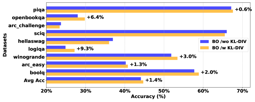
Figure 3: The performance comparison of bilevel optimization with/without KL divergence. The number on the bar indicate the accuracy improvement compared to the method without KL divergence.

C.1 Softmax Reparametrization for Score Model’s Output

In our experiment, we apply a softmax function on all batch samples’ score across GPUs to obtain the importance weights $P_{i}$. Note that the raw output of the score model is already within the range $(0,1)$, but we add another softmax function on top of it. We want to demonstrate the effectiveness of this softmax reparameterization. Intuitively, the main benefit is that it naturally amplifies important samples while downweighting less useful ones, improving the overall data selection process.

To assess the impact of the softmax reparameterization, we conduct an ablation experiment comparing two approaches: (i) naive weighting, where the raw outputs of the score model are used directly as sample weights; (ii) softmax weighting, where the softmax-transformed outputs of the score model determine the sample weights. The results, shown in Table 5, indicate that softmax weighting consistently outperforms naive weighting, leading to a 1.1% improvement in average downstream accuracy. This demonstrates that softmax effectively enhances data selection by better distinguishing important samples.

C.2 The Size of Proxy Model

We conduct experiments using two different sizes of proxy/score models (31M and 160M) for a 410M LLM. We observe that the KL divergence between the proxy and the LLM remains low for both sizes-0.15 for the 160M model and 0.10 for the 31M model. The corresponding learning curves are shown in Figure 7(a), which presents the results from round 2. The performance comparison of two sizes of proxy model is summarized in Table 6. These findings suggest that even a small proxy model (31M) is sufficient to serve as an effective surrogate for the 410M LLM.

(a) The evolution of the lower-level training loss and KL divergence for different proxy model size. Subfigures (a), (b): Proxy model size 31M, target LLM size 410M. Subfigures (c), (d): Proxy model size 160M, target LLM size 410M.

Table 6: Comparison of BLISS with different size of proxy/score model and on zero-shot evaluation over multiuple downstream datasets (410M model, 10B tokens) with 20k-step training.

Method	SciQ	ARC-E	ARC-C	LogiQA	OBQA	BoolQ	HellaSwag	PIQA	WinoGrande	Average
BLISS (Pythia-31M)	65.5(1.5)	40.8(1.0)	23.4(1.2)	27.2(1.7)	29.8(2.0)	58.9(0.9)	36.0(0.5)	67.6(1.1)	53.4(1.4)	44.7(1.3)
BLISS (Pythia-160M)	63.8(1.5)	40.8(1.0)	23.4(1.2)	27.5(1.8)	29.8(2.0)	51.3(0.9)	38.3(0.5)	67.6(1.1)	50.4(1.4)	44.1(1.3)

C.3 Initialization Method for the Score model

In Algorithm 1, we initialize the score model in each new round using the parameters from the last round. This design is motivated by the role of the score model: it learns data representations and ranks the importance of training samples. As training progresses, the model’s ability of feature learning improves, making it beneficial to retain learned representations across rounds.

To validate this, we conduct ablation studies comparing two cases:

1. Original BLISS (BLISS-org): the score model in each round is initialized with the parameters from the last round.

2. Modified Initialization (BLISS^†): the score model in each round is reset to its initial parameters from round 1.

We then use the trained score models from two cases to select training data and pretrain the target LLM for 15B tokens, respectively. The resulting LLMs are evaluated on multiple downstream datasets. As shown in Table 7, BLISS^† achieves an average performance that is $0.4\%$ lower than BLISS-org, demonstrating that continuous initialization leads to better data ranking and improved downstream performance.

Table 7: Comparison of methods on zero-shot evaluation over multiple downstream datasets (410M model, 15B tokens). BLISS-org denotes the original algorithm, and BLISS^† is a variant which uses different initialization method for the score model.

Methods (#FLOPs $\times 10^{19}$)	SciQ	ARC-E	ARC-C	LogiQA	OBQA	BoolQ	HellaSwag	PIQA	WinoGrande	Average
BLISS-org	67.7 (1.5)	41.7 (1.0)	23.6 (1.2)	25.8(1.7)	28.4(2.0)	56.0 (0.8)	39.7 (0.5)	68.7 (1.1)	53.2 (1.4)	44.9 (1.3)
BLISS†	65.2 (1.5)	41.6 (1.0)	23.4 (1.2)	27.1 (1.7)	29.8 (2.0)	57.5 (0.8)	34.9 (0.5)	67.7 (1.1)	53.5 (1.4)	44.5 (1.3)

C.4 Validation Datasets

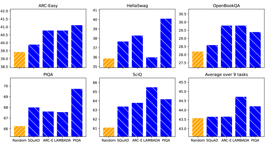
Figure 7: Comparison of BLISS trained with different validation datasets (410M model, 10B tokens). We compare our method with different validation datasets with random selection on 1 downstream task in each subplot.

The upper-level optimization aims to minimize the proxy model’s loss on the validation dataset, meaning different validation datasets influence data selection. We use different validation set, including SQUAD, ARC-E, LAMBADA, and PIQA, to conduct the bilevel data training, then compare the corresponding downstream performance.

As shown in Figure 7, our algorithm outperforms random selection on most downstream tasks, except BoolQ, regardless of the validation dataset. Notably, LAMBADA yields the highest average accuracy, improving 1.15% over random selection, likely due to its broad domain coverage.

We also notice that our averaged performance is greatly affected by the accuracy of BoolQ task across all validation datasets. This indicates that it is hard to learn when the answer is too short like yes or no.

Appendix D Additional results

Since we use the same experimental settings as MATES(Yu et al., 2024), including pretraining model, data and training steps, we evaluate MATES on the downstream tasks with their checkpoint model (https://huggingface.co/yuzc19/pythia-410m-mates/blob/main/iter-200800-ckpt.pth) of 50k steps. For other baselines, we quote Table 1 from MATES(Yu et al., 2024) for convenience of look-up for the performance of more algorithms.

Table 8: Results of Different Methods under the 410M/1B Setting. Subscripts denote standard deviations. Best scores are in bold.

Methods${}_{(\text{\#FLOPs}\ast 1e{19})}$	SciQ	ARC-E	ARC-C	LogiQA	OBQA	BoolQ	HellaSwag	PIQA	WinoGrande	Average
410M Setting: 410M model, 25B tokens
Random(6.35)	64.1(1.5)	40.2(1.0)	25.6(1.3)	24.7(1.7)	29.4(2.0)	58.9(0.9)	39.7(0.5)	67.1(1.1)	50.6(1.4)	44.5(1.3)
DSIR(6.35)	63.1(1.5)	39.9(1.0)	23.8(1.2)	27.0(1.7)	28.4(2.0)	58.3(0.9)	39.6(0.5)	66.8(1.1)	51.5(1.4)	44.3(1.3)
LESS(246.35)	64.6(1.5)	42.3(1.0)	23.1(1.2)	25.2(1.7)	30.4(2.1)	55.6(0.9)	41.9(0.5)	67.2(1.1)	51.0(1.4)	44.6(1.4)
SemDeDup(7.81)	63.5(1.5)	42.4(1.0)	24.4(1.3)	27.6(1.7)	30.0(2.1)	58.2(0.9)	40.8(0.5)	67.8(1.1)	52.3(1.4)	45.2(1.3)
DsDm(10.72)	65.4(1.5)	41.7(1.0)	24.7(1.3)	27.5(1.8)	29.0(2.1)	57.5(0.9)	40.3(0.5)	67.1(1.1)	50.1(1.4)	44.9(1.4)
QuRating(26.35)	64.8(1.5)	42.0(1.0)	25.4(1.3)	25.3(1.7)	30.2(2.1)	58.9(0.9)	40.7(0.5)	67.5(1.1)	52.1(1.4)	45.2(1.4)
MATES(8.11)	65.7(1.5)	41.5(1.0)	25.0(1.3)	26.1(1.7)	30.8(2.1)	60.6(0.9)	41.0(0.5)	67.8(1.1)	51.8(1.4)	45.7(1.4)
BLISS(8.08)	68.1(1.5)	42.2(1.0)	25.1(1.3)	27.3(1.7)	29.6(2.0)	59.3(0.9)	41.2(0.5)	68.2(1.1)	52.0(1.4)	45.9(1.4)
1B Setting: 1B model, 25B tokens
Random(17.67)	65.8(1.5)	43.7(1.0)	25.6(1.3)	27.5(1.8)	31.8(2.1)	60.2(0.9)	43.8(0.5)	68.9(1.1)	50.7(1.4)	46.4(1.4)
DSIR(17.67)	65.8(1.5)	42.6(1.0)	24.7(1.3)	28.7(1.8)	29.2(2.0)	59.7(0.9)	44.2(0.5)	68.3(1.1)	53.2(1.4)	46.3(1.4)
SemDeDup(19.13)	66.8(1.5)	45.5(1.0)	25.3(1.3)	27.6(1.8)	30.6(2.1)	60.2(0.9)	45.3(0.5)	69.7(1.1)	52.5(1.4)	47.1(1.4)
DsDm(22.04)	68.2(1.5)	45.0(1.0)	26.5(1.3)	26.6(1.7)	29.4(2.0)	59.0(0.9)	44.8(0.5)	68.9(1.1)	51.9(1.4)	46.7(1.3)
QuRating(37.67)	67.1(1.5)	45.5(1.0)	25.6(1.3)	26.9(1.7)	29.8(2.0)	60.3(0.9)	45.2(0.5)	70.2(1.1)	51.6(1.4)	46.9(1.3)
MATES(19.97)	67.3(1.5)	44.9(1.0)	25.9(1.3)	28.7(1.8)	32.2(2.1)	60.9(0.9)	45.3(0.5)	69.5(1.1)	52.4(1.4)	47.5(1.4)
BLISS(8.08)	69.4(1.5)	45.7(1.0)	24.8(1.3)	25.8(1.7)	33.2(2.1)	59.8(0.9)	47.8(0.5)	71.6(1.1)	52.9(1.4)	47.9(1.3)

Appendix E Experimental Hyperparameters

Table 9: Experimental settings

Hyperparameters	Values
Pretrain
Data set	C4
Tokens	25B
Model	Pythia-410M/1B/2.8B, LLaMA-0.5B
batch size	512
Sequence length	1024
Max learning rate	1e-3
bilevel optimization
Proxy/Score model	Pythia-31M (for 410M LLM), Pythia-160M (for 1B LLM), LLaMA-134M (for LLaMA-0.5B LLM)
$\gamma$	1e-2
$\lambda$	1e-6
batch size	16(Pythia-410M, LLaMA-0.5B)/32(Pythia 1B)
Proxy/Score model learning rate($\eta_{1}/\eta_{2}$)	1e-5
GDLS learning rate($\eta$)	1e-2
GDLS steps(K)	3
Score model steps	3k(Pythia-410M/1B)/1k(LLaMA-0.5B)
Proxy model steps	3k(Pythia-410M/1B)/1k(LLaMA-0.5B)
Initialization of score/proxy model	Randomly initialized

Table 9 shows the hyperparameter settings in our experiments. We use cosine learning rate scheduler in bilevel optimization, WSD(Yu et al., 2024) learning rate scheduler for pretraining and constant learning rate for GDLS. We use double loop to update the proxy model when employing 1B LLM, i.e., 5 steps for the lower level update. The experiments run on 8 A6000 GPUs with Distributed Data Parallel (DDP) strategy.

Appendix F Evolution of training and validation loss

In Figure F, 11(a), the training loss and validation loss correspond to the lower-level and upper-level objective functions in Equation (1), respectively.

(a) The evolution of the lower-level training loss and upper-level validation loss in round 2.

(a) The evolution of Lower-level training loss and upper-level validation loss in round 5.

(b) The visualization of lower-level training loss and the upper-level validation loss in round 2 bilevel optimization without KL divergence.

Appendix G Distributed Softmax to Compute Influence Score

In bilevel optimization, the importance weight $P_{i}$ is computed based on a mini batch that is distributed across different GPUs. However, back propagation through different GPUs is not implemented by Pytorch. Thus we deploy "distributed softmax" in practice. In detail, our implementation requires 3 times of communication among GPUs.

$$P_{i}=\frac{e^{h(\theta_{s};\xi_{i})}}{\sum_{j=1}^{B}e^{h(\theta_{s};\xi_{j})}}$$ (7)

As equation (7) shows, the denominator of $P_{i}$ is the summation of every sample’s exponential score. Therefore, in the first communication, each GPU gets the scores from others and calculates the denominator locally. A second communication is required to compute the term $\sum_{j=1}^{\mathcal{B}}P_{j}\nabla_{\theta_{s}}h(\theta_{s}^{t};\xi_{j})$ in equation (5). In detail, we need to gather gradients of $h$ and $\mathcal{L}$’ of every sample across all GPUs. After computing hyper-gradients of every sample, they are accumulated to update upper-level variables. With efficient communication API provided by Fabric https://lightning.ai/docs/fabric/stable/, the time consumed in bilevel optimization of each round is within 1.5 hours.

References

- Abbas et al. (2023) Amro Abbas, Kushal Tirumala, Dániel Simig, Surya Ganguli, and Ari S Morcos. Semdedup: Data-efficient learning at web-scale through semantic deduplication. arXiv preprint arXiv:2303.09540, 2023.
- Albalak et al. (2023) Alon Albalak, Liangming Pan, Colin Raffel, and William Yang Wang. Efficient online data mixing for language model pre-training. In R0-FoMo: Robustness of Few-shot and Zero-shot Learning in Large Foundation Models, 2023.
- Albalak et al. (2024) Alon Albalak, Yanai Elazar, Sang Michael Xie, Shayne Longpre, Nathan Lambert, Xinyi Wang, Niklas Muennighoff, Bairu Hou, Liangming Pan, Haewon Jeong, et al. A survey on data selection for language models. arXiv preprint arXiv:2402.16827, 2024.
- Bisk et al. (2020) Yonatan Bisk, Rowan Zellers, Jianfeng Gao, Yejin Choi, et al. Piqa: Reasoning about physical commonsense in natural language. In Proceedings of the AAAI conference on artificial intelligence, volume 34, pp. 7432–7439, 2020.
- Borsos et al. (2020) Zalán Borsos, Mojmir Mutny, and Andreas Krause. Coresets via bilevel optimization for continual learning and streaming. Advances in Neural Information Processing Systems, 33:14879–14890, 2020.
- Bracken & McGill (1973) Jerome Bracken and James T McGill. Mathematical programs with optimization problems in the constraints. Operations Research, 21(1):37–44, 1973.
- Brown et al. (2020) Tom Brown, Benjamin Mann, Nick Ryder, Melanie Subbiah, Jared D Kaplan, Prafulla Dhariwal, Arvind Neelakantan, Pranav Shyam, Girish Sastry, Amanda Askell, Sandhini Agarwal, Ariel Herbert-Voss, Gretchen Krueger, Tom Henighan, Rewon Child, Aditya Ramesh, Daniel M. Ziegler, Jeffrey Wu, Clemens Winter, Christopher Hesse, Mark Chen, Eric Sigler, Mateusz Litwin, Scott Gray, Benjamin Chess, Jack Clark, Christopher Berner, Sam McCandlish, Alec Radford, Ilya Sutskever, and Dario Amodei. Language models are few-shot learners. Advances in neural information processing systems, 33:1877–1901, 2020.
- Chen et al. (2023) Lesi Chen, Jing Xu, and Jingzhao Zhang. On bilevel optimization without lower-level strong convexity. arXiv preprint arXiv:2301.00712, 2023.
- Chen et al. (2024) Mayee Chen, Nicholas Roberts, Kush Bhatia, Jue Wang, Ce Zhang, Frederic Sala, and Christopher Ré. Skill-it! a data-driven skills framework for understanding and training language models. Advances in Neural Information Processing Systems, 36, 2024.
- Chowdhery et al. (2023) Aakanksha Chowdhery, Sharan Narang, Jacob Devlin, Maarten Bosma, Gaurav Mishra, Adam Roberts, Paul Barham, Hyung Won Chung, Charles Sutton, Sebastian Gehrmann, et al. Palm: Scaling language modeling with pathways. Journal of Machine Learning Research, 24(240):1–113, 2023.
- Clark et al. (2019) Christopher Clark, Kenton Lee, Ming-Wei Chang, Tom Kwiatkowski, Michael Collins, and Kristina Toutanova. Boolq: Exploring the surprising difficulty of natural yes/no questions. arXiv preprint arXiv:1905.10044, 2019.
- Clark et al. (2018) Peter Clark, Isaac Cowhey, Oren Etzioni, Tushar Khot, Ashish Sabharwal, Carissa Schoenick, and Oyvind Tafjord. Think you have solved question answering? try arc, the ai2 reasoning challenge. arXiv preprint arXiv:1803.05457, 2018.
- Conneau & Lample (2019) Alexis Conneau and Guillaume Lample. Cross-lingual language model pretraining. Advances in neural information processing systems, 32, 2019.
- Cook (1977) R Dennis Cook. Detection of influential observation in linear regression. Technometrics, 19(1):15–18, 1977.
- Dagréou et al. (2022) Mathieu Dagréou, Pierre Ablin, Samuel Vaiter, and Thomas Moreau. A framework for bilevel optimization that enables stochastic and global variance reduction algorithms. arXiv preprint arXiv:2201.13409, 2022.
- Dempe (2002) Stephan Dempe. Foundations of bilevel programming. Springer Science & Business Media, 2002.
- Du et al. (2022) Nan Du, Yanping Huang, Andrew M Dai, Simon Tong, Dmitry Lepikhin, Yuanzhong Xu, Maxim Krikun, Yanqi Zhou, Adams Wei Yu, Orhan Firat, et al. Glam: Efficient scaling of language models with mixture-of-experts. In International Conference on Machine Learning, pp. 5547–5569. PMLR, 2022.
- Elazar et al. (2023) Yanai Elazar, Akshita Bhagia, Ian Magnusson, Abhilasha Ravichander, Dustin Schwenk, Alane Suhr, Pete Walsh, Dirk Groeneveld, Luca Soldaini, Sameer Singh, et al. What’s in my big data? arXiv preprint arXiv:2310.20707, 2023.
- Engstrom et al. (2024) Logan Engstrom, Axel Feldmann, and Aleksander Madry. Dsdm: Model-aware dataset selection with datamodels. arXiv preprint arXiv:2401.12926, 2024.
- Fan et al. (2023) Simin Fan, Matteo Pagliardini, and Martin Jaggi. Doge: Domain reweighting with generalization estimation. arXiv preprint arXiv:2310.15393, 2023.
- Finn et al. (2017) Chelsea Finn, Pieter Abbeel, and Sergey Levine. Model-agnostic meta-learning for fast adaptation of deep networks. In International conference on machine learning, pp. 1126–1135. PMLR, 2017.
- Franceschi et al. (2018) Luca Franceschi, Paolo Frasconi, Saverio Salzo, Riccardo Grazzi, and Massimiliano Pontil. Bilevel programming for hyperparameter optimization and meta-learning. In International Conference on Machine Learning, pp. 1568–1577. PMLR, 2018.
- Gao et al. (2020) Leo Gao, Stella Biderman, Sid Black, Laurence Golding, Travis Hoppe, Charles Foster, Jason Phang, Horace He, Anish Thite, Noa Nabeshima, Shawn Presser, and Connor Leahy. The pile: An 800gb dataset of diverse text for language modeling. arXiv preprint arXiv:2101.00027, 2020.
- Gao et al. (2021) Leo Gao, Jonathan Tow, Stella Biderman, Sid Black, Anthony DiPofi, Charles Foster, Laurence Golding, Jeffrey Hsu, Kyle McDonell, Niklas Muennighoff, et al. A framework for few-shot language model evaluation. Version v0. 0.1. Sept, 10:8–9, 2021.
- Ghadimi & Wang (2018) Saeed Ghadimi and Mengdi Wang. Approximation methods for bilevel programming. arXiv preprint arXiv:1802.02246, 2018.
- Gong et al. (2024) Xiaochuan Gong, Jie Hao, and Mingrui Liu. A nearly optimal single loop algorithm for stochastic bilevel optimization under unbounded smoothness. In Forty-first International Conference on Machine Learning, 2024.
- Google (2024) Google. Gemini API Additional Terms of Service, 2024. URL https://ai.google.dev/gemini-api/terms. Accessed: January 30, 2025.
- Grangier et al. (2023) David Grangier, Pierre Ablin, and Awni Hannun. Bilevel optimization to learn training distributions for language modeling under domain shift. In NeurIPS 2023 Workshop on Distribution Shifts: New Frontiers with Foundation Models, 2023.
- Grazzi et al. (2022) Riccardo Grazzi, Massimiliano Pontil, and Saverio Salzo. Bilevel optimization with a lower-level contraction: Optimal sample complexity without warm-start. arXiv preprint arXiv:2202.03397, 2022.
- Hampel (1974) Frank R Hampel. The influence curve and its role in robust estimation. Journal of the american statistical association, 69(346):383–393, 1974.
- Hao et al. (2023) Jie Hao, Kaiyi Ji, and Mingrui Liu. Bilevel coreset selection in continual learning: A new formulation and algorithm. Advances in Neural Information Processing Systems, 36, 2023.
- Hao et al. (2024) Jie Hao, Xiaochuan Gong, and Mingrui Liu. Bilevel optimization under unbounded smoothness: A new algorithm and convergence analysis. In The Twelfth International Conference on Learning Representations, 2024.
- Hong et al. (2023) Mingyi Hong, Hoi-To Wai, Zhaoran Wang, and Zhuoran Yang. A two-timescale stochastic algorithm framework for bilevel optimization: Complexity analysis and application to actor-critic. SIAM Journal on Optimization, 33(1):147–180, 2023.
- Hu et al. (2021) Edward J Hu, Yelong Shen, Phillip Wallis, Zeyuan Allen-Zhu, Yuanzhi Li, Shean Wang, Lu Wang, and Weizhu Chen. Lora: Low-rank adaptation of large language models. arXiv preprint arXiv:2106.09685, 2021.
- Ji et al. (2021) Kaiyi Ji, Junjie Yang, and Yingbin Liang. Bilevel optimization: Convergence analysis and enhanced design. In International conference on machine learning, pp. 4882–4892. PMLR, 2021.
- Koh & Liang (2017) Pang Wei Koh and Percy Liang. Understanding black-box predictions via influence functions. In International conference on machine learning, pp. 1885–1894. PMLR, 2017.
- Kwon et al. (2023) Jeongyeol Kwon, Dohyun Kwon, Stephen Wright, and Robert D Nowak. A fully first-order method for stochastic bilevel optimization. In International Conference on Machine Learning, pp. 18083–18113. PMLR, 2023.
- Laurençon et al. (2022) Hugo Laurençon, Lucile Saulnier, Thomas Wang, Christopher Akiki, Albert Villanova del Moral, Teven Le Scao, Leandro Von Werra, Chenghao Mou, Eduardo González Ponferrada, Huu Nguyen, et al. The bigscience roots corpus: A 1.6 tb composite multilingual dataset. Advances in Neural Information Processing Systems, 35:31809–31826, 2022.
- Lee et al. (2021) Katherine Lee, Daphne Ippolito, Andrew Nystrom, Chiyuan Zhang, Douglas Eck, Chris Callison-Burch, and Nicholas Carlini. Deduplicating training data makes language models better. arXiv preprint arXiv:2107.06499, 2021.
- Li et al. (2024) Jeffrey Li, Alex Fang, Georgios Smyrnis, Maor Ivgi, Matt Jordan, Samir Gadre, Hritik Bansal, Etash Guha, Sedrick Keh, Kushal Arora, et al. Datacomp-lm: In search of the next generation of training sets for language models. arXiv preprint arXiv:2406.11794, 2024.
- Ling (1984) Robert F Ling. Residuals and influence in regression, 1984.
- Liu et al. (2020) Jian Liu, Leyang Cui, Hanmeng Liu, Dandan Huang, Yile Wang, and Yue Zhang. Logiqa: A challenge dataset for machine reading comprehension with logical reasoning. arXiv preprint arXiv:2007.08124, 2020.
- Maini et al. (2024) Pratyush Maini, Skyler Seto, He Bai, David Grangier, Yizhe Zhang, and Navdeep Jaitly. Rephrasing the web: A recipe for compute and data-efficient language modeling. arXiv preprint arXiv:2401.16380, 2024.
- Mihaylov et al. (2018) Todor Mihaylov, Peter Clark, Tushar Khot, and Ashish Sabharwal. Can a suit of armor conduct electricity? a new dataset for open book question answering. arXiv preprint arXiv:1809.02789, 2018.
- OpenAI (2024) OpenAI. OpenAI Terms of Service, 2024. URL https://openai.com/terms. Accessed: Jan 30, 2025.
- Oren et al. (2019) Yonatan Oren, Shiori Sagawa, Tatsunori B Hashimoto, and Percy Liang. Distributionally robust language modeling. arXiv preprint arXiv:1909.02060, 2019.
- Pan et al. (2024) Rui Pan, Jipeng Zhang, Xingyuan Pan, Renjie Pi, Xiaoyu Wang, and Tong Zhang. Scalebio: Scalable bilevel optimization for llm data reweighting. arXiv preprint arXiv:2406.19976, 2024.
- Paperno et al. (2016) Denis Paperno, Germán Kruszewski, Angeliki Lazaridou, Quan Ngoc Pham, Raffaella Bernardi, Sandro Pezzelle, Marco Baroni, Gemma Boleda, and Raquel Fernández. The lambada dataset: Word prediction requiring a broad discourse context. arXiv preprint arXiv:1606.06031, 2016.
- Park et al. (2023) Sung Min Park, Kristian Georgiev, Andrew Ilyas, Guillaume Leclerc, and Aleksander Madry. Trak: Attributing model behavior at scale. arXiv preprint arXiv:2303.14186, 2023.
- Penedo et al. (2023) Guilherme Penedo, Quentin Malartic, Daniel Hesslow, Ruxandra Cojocaru, Alessandro Cappelli, Hamza Alobeidli, Baptiste Pannier, Ebtesam Almazrouei, and Julien Launay. The refinedweb dataset for falcon llm: outperforming curated corpora with web data, and web data only. arXiv preprint arXiv:2306.01116, 2023.
- Rae et al. (2021) Jack W Rae, Sebastian Borgeaud, Trevor Cai, Katie Millican, Jordan Hoffmann, Francis Song, John Aslanides, Sarah Henderson, Roman Ring, Susannah Young, et al. Scaling language models: Methods, analysis & insights from training gopher. arXiv preprint arXiv:2112.11446, 2021.
- Raffel et al. (2020) Colin Raffel, Noam Shazeer, Adam Roberts, Katherine Lee, Sharan Narang, Michael Matena, Yanqi Zhou, Wei Li, and Peter J Liu. Exploring the limits of transfer learning with a unified text-to-text transformer. Journal of machine learning research, 21(140):1–67, 2020.
- Rajpurkar (2016) P Rajpurkar. Squad: 100,000+ questions for machine comprehension of text. arXiv preprint arXiv:1606.05250, 2016.
- Sagawa et al. (2019) Shiori Sagawa, Pang Wei Koh, Tatsunori B Hashimoto, and Percy Liang. Distributionally robust neural networks. In International Conference on Learning Representations (ICLR), 2019.
- Sakaguchi et al. (2021) Keisuke Sakaguchi, Ronan Le Bras, Chandra Bhagavatula, and Yejin Choi. Winogrande: An adversarial winograd schema challenge at scale. Communications of the ACM, 64(9):99–106, 2021.
- Shen et al. (2024) Han Shen, Pin-Yu Chen, Payel Das, and Tianyi Chen. Seal: Safety-enhanced aligned llm fine-tuning via bilevel data selection. arXiv preprint arXiv:2410.07471, 2024.
- Somayajula et al. (2023) Sai Ashish Somayajula, Lifeng Jin, Linfeng Song, Haitao Mi, and Dong Yu. Bi-level finetuning with task-dependent similarity structure for low-resource training. In Findings of the Association for Computational Linguistics: ACL 2023, pp. 8569–8588, 2023.
- Sorscher et al. (2022) Ben Sorscher, Robert Geirhos, Shashank Shekhar, Surya Ganguli, and Ari Morcos. Beyond neural scaling laws: beating power law scaling via data pruning. Advances in Neural Information Processing Systems, 35:19523–19536, 2022.
- Tirumala et al. (2023) Kushal Tirumala, Daniel Simig, Armen Aghajanyan, and Ari Morcos. D4: Improving llm pretraining via document de-duplication and diversification. Advances in Neural Information Processing Systems, 36:53983–53995, 2023.
- Welbl et al. (2017) Johannes Welbl, Nelson F Liu, and Matt Gardner. Crowdsourcing multiple choice science questions. arXiv preprint arXiv:1707.06209, 2017.
- Wenzek et al. (2019) Guillaume Wenzek, Marie-Anne Lachaux, Alexis Conneau, Vishrav Chaudhary, Francisco Guzmán, Armand Joulin, and Edouard Grave. Ccnet: Extracting high quality monolingual datasets from web crawl data. arXiv preprint arXiv:1911.00359, 2019.
- Wettig et al. (2024) Alexander Wettig, Aatmik Gupta, Saumya Malik, and Danqi Chen. Qurating: Selecting high-quality data for training language models. arXiv preprint arXiv:2402.09739, 2024.
- Xia et al. (2023) Mengzhou Xia, Tianyu Gao, Zhiyuan Zeng, and Danqi Chen. Sheared llama: Accelerating language model pre-training via structured pruning. arXiv preprint arXiv:2310.06694, 2023.
- Xia et al. (2024) Mengzhou Xia, Sadhika Malladi, Suchin Gururangan, Sanjeev Arora, and Danqi Chen. Less: Selecting influential data for targeted instruction tuning. arXiv preprint arXiv:2402.04333, 2024.
- Xie et al. (2023a) Sang Michael Xie, Hieu Pham, Xuanyi Dong, Nan Du, Hanxiao Liu, Yifeng Lu, Percy Liang, Quoc V Le, Tengyu Ma, and Adams Wei Yu. Doremi: Optimizing data mixtures speeds up language model pretraining. Advances in Neural Information Processing Systems, 2023a.
- Xie et al. (2023b) Sang Michael Xie, Shibani Santurkar, Tengyu Ma, and Percy S Liang. Data selection for language models via importance resampling. Advances in Neural Information Processing Systems, 36:34201–34227, 2023b.
- Yu et al. (2024) Zichun Yu, Spandan Das, and Chenyan Xiong. Mates: Model-aware data selection for efficient pretraining with data influence models. arXiv preprint arXiv:2406.06046, 2024.
- Zellers et al. (2019) Rowan Zellers, Ari Holtzman, Yonatan Bisk, Ali Farhadi, and Yejin Choi. Hellaswag: Can a machine really finish your sentence? arXiv preprint arXiv:1905.07830, 2019.
- Zhou et al. (2022) Xiao Zhou, Renjie Pi, Weizhong Zhang, Yong Lin, Zonghao Chen, and Tong Zhang. Probabilistic bilevel coreset selection. In International Conference on Machine Learning, pp. 27287–27302. PMLR, 2022.