A Timed Obstruction Logic for Dynamic Game Models

Abstract

Real-time cybersecurity and privacy applications require reliable verification methods and system design tools to ensure their correctness. Many of these reactive real-time applications embedded in various infrastructures, such as airports, hospitals, and oil pipelines, are potentially vulnerable to malicious cyber-attacks. Recently, a growing literature has recognized Timed Game Theory as a sound theoretical foundation for modeling strategic interactions between attackers and defenders. This paper proposes Timed Obstruction Logic (TOL), an extension of Obstruction Logic (OL), a formalism for verifying specific timed games with real-time objectives unfolding in dynamic models. These timed games involve players whose discrete and continuous actions can impact the underlying timed game model. We show that TOL can be used to describe important timed properties of real-time cybersecurity games. Finally, in addition to introducing our new logic and adapting it to specify properties in the context of cybersecurity, we provide a verification procedure for TOL and show that its complexity is PSPACE-complete, meaning that it is not higher than that of classical timed temporal logics like TCTL. Thus, we increase the expressiveness of properties without incurring any cost in terms of complexity.

1 Introduction

Multi-agent systems (MAS) are usually understood as systems composed of interacting autonomous agents [40, 4, 44, 48, 34, 35]. In this sense, MAS have been successfully applied as a modeling paradigm in several scenarios, particularly in the area of cybersecurity and distributed systems. However, the process of modeling security and heterogeneous distributed systems is inherently error-prone: thus, computer scientists typically address the issue of verifying that a system actually behaves as intended, especially for complex systems.

Some techniques have been developed to accomplish this task: testing is the most common technique, but in many circumstances, a formal proof of correctness is required. Formal verification techniques include theorem checking and model checking [22]. In particular, model checking techniques have been successfully applied to the formal verification of security and distributed systems, including hardware components, communication protocols, and security protocols. Unlike traditional distributed systems, formal verification techniques for Real-Time MAS (RT-MAS) [16, 17] are still in their infancy due to the more sophisticated nature of the agents, their autonomy, their real-time constraints, and the richness of the formalisms used to specify properties [23, 39].

RT-MAS combines game theory techniques with real-time behavior in a distributed environment [16, 17, 6]. Such real-time behavior can be verified using real-time modal logic [52, 7]. The development of methods and techniques with integrated features from both research areas undoubtedly leads to an increase in complexity and the need to adapt current techniques or, in some cases, to develop new formalisms, techniques, and tools [55, 54, 45]. Developing these formalisms correctly requires algorithms, procedures, and tools to produce reliable end results [12, 56].

Agents in RT-MAS are considered to be players in games played over real-time models (such as Timed Automata (TA) [3] and Timed Petri Nets [37]), and their goals are specified by real-time logic formulas [51, 54, 45, 37, 7]. For example, the fact that a coalition of players has a strategy to achieve a certain goal by acting cooperatively can be expressed using the syntax of logics such as Timed Alternating-time Temporal Logic (TATL) [33, 42]. For example, the fact that a coalition of players has a strategy to achieve a certain goal by acting cooperatively can be expressed using the syntax of logics such as TATL and Strategic Timed Computation Tree Logic (STCTL) [7]. However, STCTL with continuous semantics is more expressive than TATL, as shown in [7]. Moreover, in [7] was shown that the model checking problem for STCTL with continuous semantics and memoryless perfect information is of the same complexity as for TCTL, while for STCTL with continuous semantics and perfect recall is undecidable. Model checking for TATL with continuous semantics is undecidable [7]. In all previous logics, the timed game model in which the players are playing is treated as a static game model, i.e., the actions of the players affect their position within the model, but do not affect the structure of the model itself.

In this paper, we propose a new logic, Timed Obstruction Logic (TOL), for reasoning about RT-MAS with real-time goals [51, 54, 45, 37, 7] played in a dynamic model. Dynamic game models [50, 56, 19] have been studied in a variety of contexts, including cybersecurity and planning. In our new logic (TOL), games are played over an extension TA (Weighted TA (WTA) [5]) by two players (Adversary and Demon). There is a cost ($W(e)$) associated with each edge of the automaton. This means that, given a location $l$ of the automaton and a natural number $n$, the Demon deactivates an appropriate subset $T$ of the set of edges incident to $l$ such that the sum of the deactivation costs of the edges contained in $T$ is less than $n$. Then, the Adversary selects a location $l^{\prime}$ such that $l$ is adjacent to $l^{\prime}$ and the edge from $l$ to $l^{\prime}$ does not belong to the set of edges selected by the Demon in the previous round. The edges deactivated in the previous round are restored, and a new round starts at the last node selected by the opponent. The Demon wins the timed game if the infinite sequence of nodes subsequently selected by the opponent satisfies a certain property $\varphi$ expressed by a timed temporal formula. Furthermore, in addition to the introduction of our new logic and its adaptation to the specification of properties in the context of real-time cybersecurity, we provide a verification procedure for TOL and show that its complexity is PSPACE-complete, i.e., not higher than that of classical timed temporal logics such as TCTL. Thus, we increase the expressiveness of properties without incurring a cost in terms of complexity.

Structure of the work. The contribution is structured as follows. Theoretical background is presented in Section 2. In Section 3, we present the syntax and the semantics of our new logic, called Timed Obstruction Logic (TOL). In Section 4, we show our model checking algorithm and prove that the model checking problem for TOL is PSPACE-Complete. In Section 5, we compare TOL with other timed logic for strategic and temporal reasoning. In Section 6, we present our case study in the cybersecurity context. In Section 8, we compare our approach to related work. Finally, Section 9 concludes and presents possible future directions.

2 Background

General Concepts.

Let $\mathbb{N}$ be the set of natural numbers, we refer to the set of natural numbers containing $0$ as $\mathbb{N}_{\geq 0}$, $\mathbb{R}_{\geq 0}$ the set of non-negative reals and $\mathbb{Z}$ the set of integers. Let $X$ and $Y$ be two sets and $|X|$ denotes its cardinality. The set operations of intersection, union, complementation, set difference, and Cartesian product are denoted $X$ $\cap$ $Y$, $X$ $\cup$ $Y$, $\overline{X}$, $X$ $\setminus$ $Y$, and $X$ $\times$ $Y$, respectively. Inclusion and strict inclusion are denoted $X$ $\subseteq$ $Y$ and $X$ $\subset$ $Y$, respectively. The empty set is denoted $\emptyset$. Let $\pi=x_{1},\ldots,x_{n}$ be a finite sequence, $last(\pi)$ denotes the last element $x_{n}$ of $\pi$, we use $\sqsubseteq$ (resp. $\sqsubset$) to denote the prefix relation (resp. strict prefix relation). Let $\Sigma$ be a finite alphabet of actions. The set of all finite words over $\Sigma$ will be denoted by $\Sigma^{*}$. A timed action over an alphabet $\Sigma$ is a finite sequence $\theta$ = $((\sigma_{1},t_{1}),(\sigma_{2},t_{2})\cdot(\sigma_{n},t_{n}))$ of actions $\sigma_{i}$ $\in$ $\Sigma$ that are paired with non-negative real numbers $t_{i}$ $\in$ $\mathbb{R}_{\geq 0}$ such that the sequence $t=t_{1}t_{2}\cdots t_{n}$ of time-stamps is non-decreasing (i.e., $t_{i}\leq t_{i+1}$ for all $1\leq i<n$).

Attack Graphs and Moving Target Defense Mechanisms.

A malicious attack is defined as an attempt made by an attacker to gain unauthorized access to resources or to compromise the integrity of the system as related to system security controls. In this context, the Attack Graph (AG) [36][19] is one of the most popular attack models that has been created and is receiving a lot of attention recently. Leveraging an AG, it is possible to model the interactions between an attacker, and a defender able to dynamically deploy Moving Target Defense (MTD) mechanisms [21]. MTD mechanisms, such as Address Space Layout Randomization (ALSR) [47], are active defense mechanisms that use partial reconfiguration of the system to dynamically alter the attack surface and lower the attack’s chance of success. As a drawback, the activation of a MTD countermeasure has an impact on system performance: during the reconfiguration phase the services of the system are partially or not available. It is therefore critical to be able to select MTD deployment strategies both minimizing the residual cybersecurity risks and the negative impact on the performance of the system.

2.1 Weighted Transition Systems

Weighted Transition Systems (WTS) are an extension of the standard notion of (Labeled) Transition Systems (LTS) [53], which has been used to introduce operational semantics for a variety of reactive systems. An AG can be defined as a WTS.

Definition 1 (Weighted Transition Systems (WTS)).

Let $\mathsf{AP}$ be a finite set of atomic propositions. A WTS is a tuple $\mathcal{M}=(\textit{S},\textit{s}_{0},\Sigma,\textit{E},\textit{W},K,\textit{F})$ where:

• $S$ is a finite set of states,

• $s_{0}\in S$ is an initial state,

• $\Sigma$ is a finite set of actions,

• $E\subseteq S\times\Sigma\times S$ is a transition relation,

• $W$: $E\to\mathbb{N}_{\geq 0}$ is a function that labels the elements of $E$,

• $K$: $S\to 2^{\mathsf{AP}}$ is a labeling function for the states,

• $F\subseteq S$ is a set of goal states.

The transitions from state to state of a WTS are noted in the following way: we write $\textit{s}\xrightarrow[w]{a}\textit{s}^{\prime}$ whenever $a$ $\in$ $\Sigma$, $(s,a,s^{\prime})$ $\in$ $E$ and $W(s,a,s^{\prime})$ $=$ $w$ where $w$ $\in$ $\mathbb{N}_{\geq 0}$. A path of $\mathcal{M}$ can be defined as a finite (resp. infinite) sequence of moves: $\varrho$ = $s_{0}\xrightarrow[w_{1}]{\textit{a}_{1}}s_{1}\xrightarrow[w_{2}]{\textit{a}_{2}}s_{2}\ldots s_{n-2}\xrightarrow[w_{n-1}]{\textit{a}_{n-1}}s_{n-1}$, where $\forall 0\leq i\leq n-1$, $\forall j\geq 1,$ $w_{j}$ $\in$ $\mathbb{R}_{\geq 0}$ and $a_{j}\in\Sigma$. A path is initial if it starts in $s_{0}$. Thus, an initial path describes one execution of the system. A (Weighted) trace from $\varrho$ is a sequence $((a_{1},w_{1}),(a_{2},w_{2}),\ldots,(a_{n},w_{n}))$ of pairs $(a_{i},w_{i})$ $\in$ $\Sigma\times\mathbb{R}_{\geq 0}$ for which there exists a path $\varrho$ from which $w_{i}$ = $W(s_{i},a_{i},s_{i+1})$.

Example 1.

Figure 1 gives an example of a WTA. States of the WTA are denoted as $s_{i}$, with $0\leq i\leq 5$, attack actions and weighted as edge labels $a_{j}$, with $1\leq j\leq 7$, $w_{j}$, with $1\leq j\leq 11$.

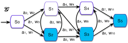
Figure 1: A WTS where states $s_{2},\,s_{3}$ and $s_{5}$ represents the goal states of the attacker.

Clocks and Timed Automata.

We use non-negative real-valued variables known as clocks to represent the continuous time domain. Clocks are variables that advance synchronously at a uniform rate; they are the basis of TA [3]. Model checkers such as UPPAAL [9], KRONOS [15], and HYTECH [30] support and extend TA. Clock constraints within TA control transitions. Here, we work with an extension of TA known as Weighted Timed Automata (WTA) [5].

2.2 Weighted Timed Automata

We now explore the relation between WTS and Weighted Timed Automata (WTA) [5]. A WTA is an extension of a TA [3] with weight/cost information at both locations and edges, and it can be used to address several interesting questions [14, 5].

Definition 2 (Clock constraints and invariants).

Let X be a finite set of clock variables ranging over $\mathbb{R}_{\geq 0}$ (non-negative real numbers). Let $\Phi(\textit{X})$ be a set of clock constraints over X. A clock constraint $\phi\in\Phi(X)$ can be defined by the following grammar:

$\phi::=true\ |\ \textit{x}\sim\textit{c}\ |\ \phi_{1}\ \wedge\ \phi_{2}$

where $\textit{x}\in\textit{X}$, $\textit{c}\in\mathbb{N}$, and $\sim\in\{<,>,\leq,\geq,=\}$.

Clock invariants $\Delta(\textit{X})$ are clock constraints in which $\sim\in\{<,\leq\}$.

Definition 3 (Clock valuations).

Given a finite set of clocks X, a clock valuation function, $\nu:\textit{X}\to\mathbb{R}_{\geq 0}$ assigning to each clock $x$ $\in$ X a non-negative value $\nu(x)$. We denote $\mathbb{R}_{\geq 0}^{X}$ the set of all valuations. For a clock valuation $\nu\in\mathbb{R}_{\geq 0}^{X}$ and a time value $\textit{d}\in\mathbb{R}_{\geq 0}$, $\nu+\textit{d}$ is the valuation satisfied by $(\nu+d)(x)=\nu(x)+d$ for each $x$ $\in$ X. Given a clock subset $Y\subseteq X$, we denote $\nu[Y\leftarrow 0]$ the valuation defined as follows: $\nu[Y\leftarrow 0](x)=0$ if $x\in Y$ and $\nu[\textit{Y}\leftarrow 0](x)=\nu(x)$ otherwise.

Here, we only consider the weight/cost in the edges (transitions) in our WTA. Formally, a WTA is defined as follows [5].

Definition 4 (Weighted Timed Automata (WTA)).

Let $X$ be a finite set of clocks and $\mathsf{AP}$ a finite set of atomic propositions. A WTA is a tuple $\mathcal{A}$ = $(L,l_{0},X,\Sigma,T,I,W,K,F)$, where:

• $L$ is a finite set of locations,

• $l_{0}\in L$ is an initial location,

• $X$ is a finite set of clocks,

• $\Sigma$ is a finite set of actions,

• $T\subseteq L\times\Sigma\times\Phi(X)\times 2^{X}\times L$ is a finite set of edges (or transitions),

• $I:L\rightarrow\Delta(X)$ is a function that associates to each location a clock invariant,

• $W$: $T\to\mathbb{N}_{\geq 0}$ is a function that labels the elements of $T$,

• $K:L\to 2^{\mathsf{AP}}$ is a labeling function for the locations,

• $F\subseteq L$ is a set of goal locations.

We write $\textit{l}\xrightarrow[w]{a,\phi,Y}\textit{l}^{\prime}$ instead of $(l,a,\phi,Y,l^{\prime})_{w}$ $\in T$ for an edge from $l$ to $l^{\prime}$ with guard $\phi$ $\in$ $\Phi(X)$, reset set $Y$ $\subseteq$ $X$ and $w$ $\in$ $\mathbb{N}_{\geq 0}$. The value $W(t)$ given to edge $t$ = $(l,a,\phi,Y,l^{\prime})_{w}$ where $t$ $\in$ $T$ represents the cost of taking that edge. In this paper, the value $W(t)$ given to edge $t$ represents the deactivation cost. Since cost information cannot be employed as constraints on edges, the undecidability of Hybrid Automata (HA) [30] is avoided in the case of WTA [14] (i.e., decidability results are preserved for WTA). In WTA, costs are explicitly defined in its syntax, however, they do not influence the discrete behavior of the system. Since there is no cost constraint, the semantics of a WTA is similar to that of a TA. It is thus given as a WTS.

Definition 5 (Semantics of WTA).

Let $\mathcal{A}=(L,l_{0},X,\Sigma,T,I,W,K,F)$ be a WTA. The semantics of WTA $\mathcal{A}$ is given by a WTS$({\mathcal{A}})$ = $(\textit{S},\textit{s}_{0},\Sigma_{\Delta},E,W^{\prime},K^{\prime},\textit{S}_{F})$ where:

• $S\subseteq L$ $\times$ $\mathbb{R}^{\textit{X}}_{\geq 0}$ is a set of states,

• $s_{0}=(l_{0},\nu_{0})$ with $\nu_{0}(x)=0$ for all $x\in\textit{X}$ and $\nu_{0}$ $\models$ $I(l_{0})$,

• $S_{F}\subseteq F$ $\times$ $\mathbb{R}^{\textit{X}}_{\geq 0}$ is a set of states,

• $\Sigma_{\Delta}$ = $\Sigma$ $\uplus$ $\mathbb{R}_{\geq 0}$,

• $W^{\prime}$ = $W$,

• $K^{\prime}((l,\nu))$ = $K(l)$ $\cup$ $\{\phi\in\Phi(X)\mid\nu\models\phi\}$,

• $E\subseteq S\times\Sigma_{\Delta}\times S$ is a transition relation defined by the following two rules:

  • Discrete transition: $(l,\nu)\xrightarrow[w]{a}(l^{\prime},\nu^{\prime})$ for $a\in\Sigma$ and $w$ $\in$ $\mathbb{N}_{\geq 0}$ iff $\textit{l}\xrightarrow[w]{a,\phi,Y}\textit{l}^{\prime}$, $\nu$ $\models$ $\phi$, $\nu^{\prime}$ $=$ $\nu[Y\leftarrow 0]$ and $\nu^{\prime}$ $\models$ $\textit{I}(l^{\prime})$ and,

  • Delay transition: $(l,\nu)\xrightarrow{d}(l,\nu+d)$, for some $d\in\mathbb{R}_{\geq 0}$ iff $\nu+d$ $\models$ $\textit{I}(l)$.

2.3 Paths and n-strategy

A path $\rho$ in $\textsf{WTS}(\mathcal{A})$ is an infinite sequence of consecutive delays and discrete transitions. A finite path fragment of $\mathcal{A}$ is a run in WTS($\mathcal{A}$) starting from the initial state $s_{0}=(l_{0},\nu_{0})$, with delay and discrete transitions alternating along the path: $\rho$ = $s_{0}\xrightarrow{d_{0}}s_{1}^{\prime}\xrightarrow[w_{0}]{\textit{a}_{0}}s_{1}\xrightarrow{d_{1}}s_{2}^{\prime}\xrightarrow[w_{1}]{\textit{a}_{1}}s_{2}\ldots s_{n-1}\xrightarrow{d_{n-1}}s_{n}^{\prime}\xrightarrow[w_{n}]{a_{n}}s_{n}$ $\ldots$ or more compactly $s_{0}\xrightarrow[w_{0}]{d_{0},a_{0}}s_{1}\xrightarrow[w_{1}]{d_{1},\textit{a}_{1}}s_{2}\xrightarrow[w_{2}]{d_{2},a_{2}}s_{3}\ldots s_{n-1}\xrightarrow[w_{n-1}]{d_{n-1},a_{n-1}}s_{n}$ $\ldots$, where $\nu_{0}(x)=0$ for every $x$ $\in$ $X$. A path of WTS$({\mathcal{A}})$ is initial if $s_{0}=(l_{0},\nu_{0})$ $\in$ $S$, where $l_{0}$ $\in$ $L$, $\nu_{0}$ assigns 0 to each clock, and maximal if it ends in a goal location. We write $\rho_{i}$ to denote the $i$-th element $s_{i}=(l_{i},\nu_{i})$ of $\rho$, $\rho_{\leq i}$ to denote the prefix $s_{0},\ldots,s_{i}$ of $\rho$ and $\rho_{\geq i}$ to denote the suffix $s_{i},s_{i+1}\ldots$ of $\rho$. A history is any finite prefix of some path. We use $H$ to denote the set of histories.

Definition 6.

Let $\mathcal{A}$ be a WTA and $n$ be a natural number. Given a model WTS($\mathcal{A}$), a $n$-strategy is a function $\mathfrak{S}:H\to 2^{E}$ that, given a history $h$, returns a subset $E^{\prime}$ such that: (i) $E^{\prime}\subset E(last(h))$, (ii) $(\sum_{e\in E^{\prime}}\mathsf{W}(e))\leq n$. A memoryless $n$-strategy is a $n$-strategy $\mathfrak{S}$ such that for all histories $h$ and $h^{\prime}$ if $last(h)=last(h^{\prime})$ then $\mathfrak{S}(h)=\mathfrak{S}(h^{\prime})$.

A path $\rho$ is compatible with a $n$-strategy if for all $i$ $\geq 1$, $(\rho_{i},\sigma,\rho_{i+1})$ $\notin$ $\mathfrak{S}(\rho_{\leq i})$, where $\sigma\in\Sigma_{\Delta}$. Given a state $s=(l,\nu)$ and a $n$-strategy $\mathfrak{S}$, $Out(s,\mathfrak{S})$ refers to the set of pathways whose first state is $s$ and are consistent with $\mathfrak{S}$.

Example 2.

Let $\mathcal{M}$ be the WTA depicted in Fig 2. $\mathcal{A}$ contains ten locations: $L_{0}$ (initial) and $L_{7}$, $L_{8}$ and $L_{9}$ are the goal locations. For the sake, all locations define invariants to be true. The transition $L_{0}\xrightarrow{a,(x\leq 2),\{x:=0\}}L_{1}$ specifies that when the input action $a$ occurs and the guard $x\leq 2$ holds, this enables the transition, leading to a new current location $L_{1}$, while resetting clock variables $x:=0$ and 3 as weight/cost. The transition $L_{1}\xrightarrow{a,(x\leq 2),\{x:=0\}}L_{2}$ specifies that when the input action $b$ occurs and the guard $x<1$ holds, this enables the transition, leading to a new current location $l_{2}$, while resetting clock variables $x:=0$ and 2 as weight/cost. Likewise, the transition $L_{1}\xrightarrow{c,(2<y<3),\{y:=0\}}L_{3}$ specifies that when the input action $c$ occurs and the guard $2<y<3$ holds, this enables the transition, leading to a new current location $L_{3}$, while resetting clock variables $y:=0$ and 1 as weight/cost. Likewise, we can see the other transitions in Fig 2.

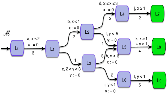
Figure 2: A WTA with two clocks $x$ and $y$.

2.4 Predecessor and Zone Graph

Since the number of states in a WTA is infinite, thus, it is impossible to build a finite state automaton. Then a symbolic semantics called zone graph was proposed for a finite representation of TA behaviors [13]. The zone graph representation of TA is not only an important implementation approach employed by most contemporary TA tools [13], but it also provides a theoretical foundation for demonstrating the decidability of semantic properties for a given TA.

In a zone graph, clock zones are used to symbolically represent sets of clock valuations. A clock zone $Z$ $\in$ $\mathbb{R}_{\geq 0}^{X}$ over a set of clocks $X$ is a set of valuations which satisfy a conjunction of constraints. Formally, the clock zone for the constraint $\phi$ is $Z$ = $\{\nu\ |\ \nu(x)\models\phi,x\in X\}$. Geometrically, a zone is a convex polyhedron. A symbolic state (or zone) is a pair $\mathcal{Z}$ = $(l,Z)$, where $l$ is a location and $Z$ is a clock zone. A zone $\mathcal{Z}$ = $(l,Z)$ represents all the states $z=(l^{\prime},\nu)$ $\in$ $\mathcal{Z}$ if $l$ = $l^{\prime}$ and $\nu$ $\in$ $Z$, indicating that a state is contained in a zone. Zones and their representation by Difference Bound Matrices (DBMs in short) are the standard symbolic data structure used in tools implementing real-time systems [13]. We can now define the symbolic discrete and delay predecessor operations on zones as follows:

Definition 7 (Discrete and Time Predecessor).

Let $\mathcal{Z}$ be a zone and $e$ be an edge of a WTS($\mathcal{A}$), then:

$$\textsf{disc-pred}(e,\mathcal{Z})=\{z\ |\ \exists z^{\prime}\in\mathcal{Z},z\xrightarrow[w]{e}z^{\prime}\}$$

$$\textsf{time-pred}(\mathcal{Z})=\{z\ |\ \exists z^{\prime}\in\mathcal{Z},z\xrightarrow[w]{d}z^{\prime}\ and\ d\in\mathbb{R}_{\geq 0}\}$$

That is, disc-$\textsf{pred}(t,\mathcal{Z})$ is the set of all $e$-predecessors of states in $\mathcal{Z}$ and time-$\textsf{pred}(\mathcal{Z})$ is the set of all time-predecessors of states in $\mathcal{Z}$. According to these definitions, if $\mathcal{Z}$ is a zone then time-$\textsf{pred}(\mathcal{Z})$ and disc-$\textsf{pred}(e,\mathcal{Z})$ are also zones, meaning that zones are preserved by the above predecessor operations.

Definition 8 (Predecessor).

Let $\mathcal{Z}$ be a zone and $e$ be a edge of a WTS($\mathcal{A}$), then :

$$\textsf{pred}(t,\mathcal{Z})=\textsf{disc-pred}(e,\textsf{time-pred}(\mathcal{Z}))$$

That is, pred is the set of all states that can reach some state in $\mathcal{Z}$ by performing a $e$ transition and allowing some time to pass.

2.5 Obstruction Logic

In this section, we recall the syntax of obstruction logic.

Definition 9.

Let $\mathsf{AP}$ be a set of atomic formulas (or atoms). Formulas of Obstruction Logic (OL) are defined by the following grammar:

$$\varphi::=\top\mid p\mid\neg\varphi\mid\varphi\land\varphi\mid\langle\textbf{\raisebox{2.15277pt}{\makebox[0.0pt][l]{\rule[-0.2pt]{3.22916pt}{0.4pt}}\makebox[3.22916pt]{\rule[-2.15277pt]{0.4pt}{6.45831pt}}}}_{n}\rangle\mathsf{X}\,\varphi\mid\langle\textbf{\raisebox{2.15277pt}{\makebox[0.0pt][l]{\rule[-0.2pt]{3.22916pt}{0.4pt}}\makebox[3.22916pt]{\rule[-2.15277pt]{0.4pt}{6.45831pt}}}}_{n}\rangle(\varphi\,\mathsf{U}\,\varphi)\mid\langle\textbf{\raisebox{2.15277pt}{\makebox[0.0pt][l]{\rule[-0.2pt]{3.22916pt}{0.4pt}}\makebox[3.22916pt]{\rule[-2.15277pt]{0.4pt}{6.45831pt}}}}_{n}\rangle(\varphi\,\mathsf{R}\,\varphi)$$

where $p$ is an atomic formula and $n$ is any number in $\mathbb{N}_{\geq 0}$.

The number $n$ is called the grade of the strategic operator. The boolean connectives $\bot$, $\vee$ and $\to$ can be defined as usual. The meaning of a formula $\langle\textbf{\raisebox{2.22221pt}{\makebox[0.0pt][l]{\rule[-0.2pt]{3.33333pt}{0.4pt}}\makebox[3.33333pt]{\rule[-2.22221pt]{0.4pt}{6.66666pt}}}}\rangle\varphi$ with $\varphi$ temporal formula is: there is a demonic strategy (that is, a strategy for disabling arcs) such that all paths of the graphs that are compatible with the strategy satisfy $\varphi$.

3 Timed Obstruction Logic

In this section, we define the syntax and semantics of our Timed Obstruction Logic (TOL). Our definitions are based on [20, 18, 19].

Definition 10.

Let $\mathcal{A}$ be a WTA, $\mathsf{AP}$ a set of atomic propositions (or atoms), a set $X$ of clocks of $\mathcal{A}$ and $J$ a non-empty set of clocks of the formula, where $X$ $\cap$ $J$ = $\emptyset$. Formulas of Timed Obstruction Logic (TOL) are defined by the following grammar:

$$\varphi::=\top\mid p\mid\neg\varphi\mid\varphi_{1}\land\varphi_{2}\mid\phi\mid\langle\textbf{\raisebox{2.15277pt}{\makebox[0.0pt][l]{\rule[-0.2pt]{3.22916pt}{0.4pt}}\makebox[3.22916pt]{\rule[-2.15277pt]{0.4pt}{6.45831pt}}}}_{n}\rangle(\varphi_{1}\,\mathsf{U}\,\ \varphi_{2})\mid\langle\textbf{\raisebox{2.15277pt}{\makebox[0.0pt][l]{\rule[-0.2pt]{3.22916pt}{0.4pt}}\makebox[3.22916pt]{\rule[-2.15277pt]{0.4pt}{6.45831pt}}}}_{n}\rangle(\varphi_{1}\,\mathsf{R}\,\ \varphi_{2})\mid j.\varphi$$

where $p$ $\in$ $\mathsf{AP}$ is an atomic formula, $j$ $\in$ $J$, $n$ $\in$ $\mathbb{N}_{\geq 0}$ represents the grade of the strategic operator, and $\phi$ $\in$ $\Phi(X\cup J)$.

It is possible to compare a formula clock and an automata clock, for example, by using the clock constraint $\phi$, which applies to both formula clocks and clocks of the TA. The boolean connectives $\bot$, $\vee$ and, $\to$ can be defined as usual. Clock $j$ in $j.\varphi$ is called a freeze identifier and bounds the formula clock $j$ in $\varphi$. The interpretation is that $j.\varphi$ is valid in a state $s$ if $\varphi$ holds in $s$ where clock $j$ starts with value 0 in $s$. This freeze identifier can be used in conjunction with temporal constructs to indicate common timeliness requirements such as punctuality, bounded response, and so on. As OL, we define $\langle\textbf{\raisebox{2.22221pt}{\makebox[0.0pt][l]{\rule[-0.2pt]{3.33333pt}{0.4pt}}\makebox[3.33333pt]{\rule[-2.22221pt]{0.4pt}{6.66666pt}}}}_{n}\rangle\mathsf{F}\,\varphi:=\langle\textbf{\raisebox{2.22221pt}{\makebox[0.0pt][l]{\rule[-0.2pt]{3.33333pt}{0.4pt}}\makebox[3.33333pt]{\rule[-2.22221pt]{0.4pt}{6.66666pt}}}}_{n}\rangle(\top\,\mathsf{U}\,\varphi)$, $\langle\textbf{\raisebox{2.22221pt}{\makebox[0.0pt][l]{\rule[-0.2pt]{3.33333pt}{0.4pt}}\makebox[3.33333pt]{\rule[-2.22221pt]{0.4pt}{6.66666pt}}}}_{n}\rangle\mathsf{G}\,\varphi:=\langle\textbf{\raisebox{2.22221pt}{\makebox[0.0pt][l]{\rule[-0.2pt]{3.33333pt}{0.4pt}}\makebox[3.33333pt]{\rule[-2.22221pt]{0.4pt}{6.66666pt}}}}_{n}\rangle(\bot\,\mathsf{R}\,\varphi)$ and $\langle\textbf{\raisebox{2.22221pt}{\makebox[0.0pt][l]{\rule[-0.2pt]{3.33333pt}{0.4pt}}\makebox[3.33333pt]{\rule[-2.22221pt]{0.4pt}{6.66666pt}}}}_{n}\rangle(\varphi\,\mathsf{W}\,\psi):=\langle\textbf{\raisebox{2.22221pt}{\makebox[0.0pt][l]{\rule[-0.2pt]{3.33333pt}{0.4pt}}\makebox[3.33333pt]{\rule[-2.22221pt]{0.4pt}{6.66666pt}}}}_{n}\rangle(\psi\,\mathsf{R}\,(\varphi\vee\psi))$. The size $|\varphi|$ of a formula $\varphi$ is the number of its connectives. With the help of the freeze identifier operator of TOL, a time constraint can be added concisely. For instance, the formula $j.\langle\textbf{\raisebox{2.22221pt}{\makebox[0.0pt][l]{\rule[-0.2pt]{3.33333pt}{0.4pt}}\makebox[3.33333pt]{\rule[-2.22221pt]{0.4pt}{6.66666pt}}}}_{n}\rangle((\varphi_{1}\wedge j\leq 7)\,\mathsf{U}\,\varphi_{2})$ intuitively means that there is a demonic strategy such that all paths that are compatible with the strategy, the property $\varphi_{1}$ holds continuously until within 7 time units $\varphi_{2}$ becomes valid. From the above formula, it is clear that timing constraints are allowed. In this case, we will call the formulas with timing constraints, such as timed temporal formulas. The intuitive meaning of a formula $\langle\textbf{\raisebox{2.22221pt}{\makebox[0.0pt][l]{\rule[-0.2pt]{3.33333pt}{0.4pt}}\makebox[3.33333pt]{\rule[-2.22221pt]{0.4pt}{6.66666pt}}}}\rangle\varphi$ with $\varphi$ timed temporal formula is: there is a demonic strategy such that all paths of the WTS that are compatible with the strategy satisfy $\varphi$. Formulas of TOL will be interpreted over WTS. We can now precisely define the semantics of TOL formulas.

Definition 11 (TOL Semantics).

Let $\mathcal{A}$ = $(L,l_{0},X,\Sigma,T,I,W,K,F)$ be a WTA, $p$ $\in$ $AP$, $\phi$ $\in$ $\Phi(X)$, $\mathcal{M}$ = WTS($\mathcal{A}$). The satisfaction relation between a WTS $\mathcal{M}$, a state $s$ = $(l,\nu)$ of $\mathcal{M}$, and TOL formulas $\varphi$ and $\psi$ is given inductively as follows:

• $\mathcal{M},s\models\top$ for all state $s$,

• $\mathcal{M},s\models p$ iff $p\in K(s)$,

• $\mathcal{M},s\models\neg\varphi$ iff not $\mathcal{M},s\models\varphi$ (notation $\mathcal{M},s\not\models\varphi$),

• $\mathcal{M},s\models\varphi_{1}$ $\wedge$ $\varphi_{2}$ iff $\mathcal{M},s\models\varphi_{1}$ and $\mathcal{M},s\models\varphi_{2}$,

• $\mathcal{M},s\models\phi$ iff $\nu\models\phi$,

• $\mathcal{M},s\models\langle\textbf{\raisebox{2.15277pt}{\makebox[0.0pt][l]{\rule[-0.2pt]{3.22916pt}{0.4pt}}\makebox[3.22916pt]{\rule[-2.15277pt]{0.4pt}{6.45831pt}}}}_{n}\rangle(\varphi\,\mathsf{U}\,\psi)$ iff there is a $n$-strategy $\mathfrak{S}$ such that for all $\rho\in Out(s,\mathfrak{S})$ there is a $j\in\mathbb{N}$ such that $\mathcal{M},\rho_{j}\models\psi$ and for all $0\leq k<j$, $\mathcal{M},\rho_{k}\models\varphi$,

• $\mathcal{M},s\models\langle\textbf{\raisebox{2.15277pt}{\makebox[0.0pt][l]{\rule[-0.2pt]{3.22916pt}{0.4pt}}\makebox[3.22916pt]{\rule[-2.15277pt]{0.4pt}{6.45831pt}}}}_{n}\rangle(\varphi\,\mathsf{R}\,\psi)$ iff there is a $n$-strategy $\mathfrak{S}$ such that for all $\rho\in Out(s,\mathfrak{S})$ we have that either $\mathcal{M},\rho_{i}\models\psi$ for all $i\in\mathbb{N}$ or there is a $k\in\mathbb{N}$ such that $\mathcal{M},\rho_{k}\models\varphi$ and $\mathcal{M},\rho_{i}\models\psi$ for all $0\leq i\leq k$,

• $\mathcal{M},s\models j.\varphi$ iff $\mathcal{M},(l,\nu[j\leftarrow 0])\models\varphi$.

Two formulas $\varphi$ and $\psi$ are semantically equivalent (denoted by $\varphi\equiv\psi$) iff for any model $\mathcal{M}$ and state $s$ of $\mathcal{M}$, $\mathcal{M},s\models\varphi$ iff $\mathcal{M},s\models\psi$. Let $\varphi$ be any formula, $X$ a set of clocks and $\mathcal{A}$ be a WTA, then Sat$({\varphi})$ denotes the set of states of $\mathcal{M}$ = $\textsf{WTS}(\mathcal{A})$ verifying, $\varphi$, i.e., Sat$(\varphi)=\{s\in S\ \,|\,\ \mathcal{M},s\models\varphi\}$. Next, we can establish the relationship between local model checking and global model checking.

Definition 12.

Given $\mathcal{M}$, $s$, and $\varphi$, the local model checking concerns determining whether $\mathcal{M},s\models\varphi$. Given $\mathcal{M}$ and $\varphi$, the global model checking concerns determining the set Sat$(\varphi)$.

Definition 13.

A state $s$ in a WTS$(\mathcal{A})$ satisfies a formula $\varphi$ iff $(s,\mu_{0})$ $\models$ $\varphi$ where $\mu_{0}$ is the clock valuation that maps each formula clock to zero.

The relationship between WTA and WTS is defined as follows.

Definition 14.

Let $\mathcal{A}$ be a WTA and $\varphi$ $\in$ TOL, then $\mathcal{A}$ $\models$ $\varphi$ iff $\textsf{WTS}(\mathcal{A})$ $\models$ $\varphi$.

Let $\varphi$ be a formula, then the set of extended states satisfying $\varphi$ is independent of the valuation $\mu$ for the formula clocks. Thus, if $\varphi$ is a formula, then for any state $s$ = $(l,\nu)$ in a WTS and valuations $\mu$, $\mu^{\prime}$ for the formula clocks, we can get that $\mathcal{M},(l,\mu)\models$ $\varphi$ iff $\mathcal{M},(l,\mu^{\prime})\models$ $\varphi$. Therefore, it makes sense to talk about a state $s$ that satisfies $\varphi$.

4 Model Checking

Here, we present our model checking algorithm for TOL. Furthermore, we show that the model checking problem for TOL is decidable in PSPACE-complete. The general structure of the algorithm shown here is similar to OL model checking algorithm [20]. TOL model checking algorithm is based on the computation of the set Sat$(\varphi)$ of all states satisfying a TOL formula $\varphi$, followed by checking whether the initial state is included in this set. A WTA $\mathcal{A}$ satisfies TOL state formula $\varphi$ if and only if $\varphi$ holds in the initial state of WTA: $\mathcal{A}\models\varphi$ if and only if $l_{0}\in L$ such that, $(l_{0},\nu_{0})$ $\in$ Sat($\varphi$), where $\nu_{0}(x)=0$ for all $x\in X$. In our TOL, a TOL formula $\langle\textbf{\raisebox{2.22221pt}{\makebox[0.0pt][l]{\rule[-0.2pt]{3.33333pt}{0.4pt}}\makebox[3.33333pt]{\rule[-2.22221pt]{0.4pt}{6.66666pt}}}}_{n}\rangle((\varphi\,\mathsf{U}\,\psi)$ holds in a state $s$ iff $\textbf{\raisebox{2.22221pt}{\makebox[0.0pt][l]{\rule[-0.2pt]{3.33333pt}{0.4pt}}\makebox[3.33333pt]{\rule[-2.22221pt]{0.4pt}{6.66666pt}}}}_{n}\textsf{U}(\textsf{Sat}(\psi_{1}),\textsf{Sat}(\psi_{2}))$ with $\,\mathsf{U}\,$ being an TOL operator. As mentioned in subsection 2.4, build a WTS($\mathcal{A}$) for some WTA $\mathcal{A}$ is therefore not practicable. Instead, the basic idea is to construct a zone graph [13], which is built from the WTA $\mathcal{A}$ and the TOL formula $\varphi$ (i.e., ZG($\mathcal{A}$, $\varphi$)). In short, Algorithm 1 begins with a WTA $\mathcal{A}$ and a formula $\varphi$ used to construct the zone graph ZG($\mathcal{A}$, $\varphi$) and returns the set of states of $\mathcal{A}$ satisfying $\varphi$. The Algorithm 1 works as follows: it first constructs the zone graph ZG($\mathcal{A}$, $\varphi$), then it recursively computes, for all subformulas $\psi$, the sets of states Sat$(\psi)$ for which $\psi$ is satisfied. The computation of Sat$(\psi)$ for $\psi$ being true, a proposition $p$, or a clock constraint $\phi$ is explicit. The negation and conjunction computations are straightforward. The computation of the TOL formula $\langle\textbf{\raisebox{2.22221pt}{\makebox[0.0pt][l]{\rule[-0.2pt]{3.33333pt}{0.4pt}}\makebox[3.33333pt]{\rule[-2.22221pt]{0.4pt}{6.66666pt}}}}_{n}\rangle(\psi_{1}\,\mathsf{U}\,\psi_{2})$ and $\langle\textbf{\raisebox{2.22221pt}{\makebox[0.0pt][l]{\rule[-0.2pt]{3.33333pt}{0.4pt}}\makebox[3.33333pt]{\rule[-2.22221pt]{0.4pt}{6.66666pt}}}}_{n}\rangle(\psi_{1}\,\mathsf{R}\,\psi_{2})$ are defined under the computation of predecessor sets. However, the notion of predecessors is different for the quantifiers in TCTL [3]. The computation of the TOL formula $\langle\textbf{\raisebox{2.22221pt}{\makebox[0.0pt][l]{\rule[-0.2pt]{3.33333pt}{0.4pt}}\makebox[3.33333pt]{\rule[-2.22221pt]{0.4pt}{6.66666pt}}}}_{n}\rangle(\psi_{1}\,\mathsf{U}\,\psi_{2})$ can be reduced to the computation of an OL formula. The computation of $\langle\textbf{\raisebox{2.22221pt}{\makebox[0.0pt][l]{\rule[-0.2pt]{3.33333pt}{0.4pt}}\makebox[3.33333pt]{\rule[-2.22221pt]{0.4pt}{6.66666pt}}}}_{n}\rangle((\psi_{1}\,\mathsf{U}\,\ \psi_{2})$ is a fixed-point iteration that starts at Sat$(\psi_{2})$ and iteratively adds all predecessor states that are in Sat$(\psi_{1})$. We need to define a new predecessor operator to compute all predecessors with the obstruction operator. We will now use our zone graph to compute predecessors. The predecessor computation is done by the operator $\blacktriangledown(n,\mathcal{Z})$ for a symbolic state $\mathcal{Z}$ (zones) and a number $n$, computes the set of all predecessor states (likewise, for the operator $\,\mathsf{R}\,$).

Definition 15.

Given a symbolic state $\mathcal{Z}$ and $e$ an edge, we define $\textsf{Pred}(\mathcal{Z})$ = $\bigcup_{e\in E}$ $\textsf{pred}(e,\mathcal{Z})$.

Therefore, the obstruction predecessor of a zone $\mathcal{Z}$, denoted $\blacktriangledown(n,\mathcal{Z})$, is defined as the set of symbolic states that characterizes all predecessors of the symbolic state $\mathcal{Z}$, where each state $z$ satisfies $\blacktriangleright(z,n,\overline{\mathcal{Z}})$, that is, it can transition to a state not in the set $\mathcal{Z}$ where the sum of all successors of $s$ is less than or equal to $n$.

Definition 16.

Let $n\in\mathbb{N}$ and $\mathcal{Z}$ a symbolic state, we write:

$$\blacktriangleright(z,n,\mathcal{Z})\ =\ (\sum_{z^{\prime}\ \in\ \mathcal{Z}\ \land\ \sigma\ \in\ \Sigma_{\Delta}}\mathsf{W}(z,\sigma,z^{\prime}))\leq n$$

$$\blacktriangledown(n,\mathcal{Z})=\{z\in\textsf{Pred}(\mathcal{Z})\,\ |\,\blacktriangleright(z,n,\overline{\mathcal{Z}})\}$$

Proposition 1.

Let $z$ a state, $n$ a natural number, and $\mathcal{Z}$ a symbolic state (or zone), then $z$ $\in$ $\blacktriangledown(n,\mathcal{Z})$ iff $z$ $\in$ $\mathcal{Z}$.

Proof.

(Sketch). A proof of this proposition may be obtained from the convexity of zones on TA [3, 57]. ∎

Proposition 2.

Let $z$ a state, $n$ a natural number, and $\mathcal{Z}$ a symbolic state, then if $\mathcal{Z}$ is convex, then $\blacktriangledown(n,\mathcal{Z})$ is also convex.

Proof.

(Sketch). A proof of this proposition may be obtained from the convexity of zones on TA [3, 57]. ∎

Algorithm 1 TOL model checking
Input: A ZG($\mathcal{A}$, $\varphi$) where $\mathcal{A}$ is a WTA and $\varphi$ is a TOL formula
Output: Sat$(\phi)$ $\leftarrow$ $\{s\in S\ |\ s\models\varphi\}$

1:for all i $\leq$ $|\varphi|$ do

2:  for all $\psi$ $\in Sub(\varphi)\ with\ |\psi|=i$ do

3:   switch $(\psi)$ do

4:     case $\psi=\top$

5:      $\textsf{Sat}(\psi)\leftarrow S$      

6:     case $\psi=p$

7:      $\textsf{Sat}(\psi)\leftarrow\{s\in S\,|\,p\in K(s)\}$      

8:     case $\psi=\neg\psi_{1}$

9:      $\textsf{Sat}(\psi)\leftarrow S\setminus\textsf{Sat}(\psi)$      

10:     case $\psi=\phi$

11:      $\textsf{Sat}(\psi)\leftarrow\phi$      

12:     case $\psi=\psi_{1}\land\psi_{2}$

13:      $\textsf{Sat}(\psi)\leftarrow\textsf{Sat}(\psi_{1})\cap\textsf{Sat}(\psi_{2})$      

14:     case $\psi=\langle\textbf{\raisebox{2.22221pt}{\makebox[0.0pt][l]{\rule[-0.2pt]{3.33333pt}{0.4pt}}\makebox[3.33333pt]{\rule[-2.22221pt]{0.4pt}{6.66666pt}}}}_{n}\rangle(\psi_{1}\,\mathsf{U_{J}}\,\psi_{2})$

15:      $\textsf{Sat}(\psi)\leftarrow{\textbf{\raisebox{2.22221pt}{\makebox[0.0pt][l]{\rule[-0.2pt]{3.33333pt}{0.4pt}}\makebox[3.33333pt]{\rule[-2.22221pt]{0.4pt}{6.66666pt}}}}_{n}}\textsf{U}(\textsf{Sat}(\psi_{1}),\textsf{Sat}(\psi_{2}))$      

16:     case $\psi=\langle\textbf{\raisebox{2.22221pt}{\makebox[0.0pt][l]{\rule[-0.2pt]{3.33333pt}{0.4pt}}\makebox[3.33333pt]{\rule[-2.22221pt]{0.4pt}{6.66666pt}}}}_{n}\rangle(\psi_{1}\,\mathsf{R_{J}}\,\psi_{2})$

17:      $\textsf{Sat}(\psi)\leftarrow\textbf{\raisebox{2.22221pt}{\makebox[0.0pt][l]{\rule[-0.2pt]{3.33333pt}{0.4pt}}\makebox[3.33333pt]{\rule[-2.22221pt]{0.4pt}{6.66666pt}}}}_{n}\textsf{R}(\textsf{Sat}(\psi_{1}),\textsf{Sat}(\psi_{2}))$      

18:     case $\psi=j.\psi_{1}$

19:      $\textsf{Sat}(\psi)\leftarrow\textsf{Sat}(\psi_{1})$           

For the $\,\mathsf{U}\,$ and $\,\mathsf{R}\,$ operators, auxiliary methods are defined. These methods are listed in Algorithm 2 and Algorithm 3. Algorithm 2 shows the backward search for computing the method ${\textbf{\raisebox{2.22221pt}{\makebox[0.0pt][l]{\rule[-0.2pt]{3.33333pt}{0.4pt}}\makebox[3.33333pt]{\rule[-2.22221pt]{0.4pt}{6.66666pt}}}}_{n}}\textsf{U}(\textsf{Sat}(\psi_{1}),\textsf{Sat}(\psi_{2}))$ in line $15$ of Algorithm 1.

Algorithm 2 Backward search for computing ${\textbf{\raisebox{2.22221pt}{\makebox[0.0pt][l]{\rule[-0.2pt]{3.33333pt}{0.4pt}}\makebox[3.33333pt]{\rule[-2.22221pt]{0.4pt}{6.66666pt}}}}_{n}}\textsf{U}$
Input: A TOL formula $\langle\textbf{\raisebox{2.22221pt}{\makebox[0.0pt][l]{\rule[-0.2pt]{3.33333pt}{0.4pt}}\makebox[3.33333pt]{\rule[-2.22221pt]{0.4pt}{6.66666pt}}}}_{n}\rangle(\psi_{1}\,\mathsf{U}\,\psi_{2})$
Output: Sat$(\langle\textbf{\raisebox{2.22221pt}{\makebox[0.0pt][l]{\rule[-0.2pt]{3.33333pt}{0.4pt}}\makebox[3.33333pt]{\rule[-2.22221pt]{0.4pt}{6.66666pt}}}}_{n}\rangle(\psi_{1}\,\mathsf{U}\,\psi_{2}))$ $\leftarrow$ $\{s\in S\ |\ s\models\langle\textbf{\raisebox{2.22221pt}{\makebox[0.0pt][l]{\rule[-0.2pt]{3.33333pt}{0.4pt}}\makebox[3.33333pt]{\rule[-2.22221pt]{0.4pt}{6.66666pt}}}}_{n}\rangle(\psi_{1}\,\mathsf{U}\,\psi_{2})\}$

1:$X\leftarrow\emptyset$

2:$Y\leftarrow\psi_{2}$

3:while $Y\neq X$ do

4:  $X\leftarrow Y$

5:  $Y\leftarrow\psi_{2} \cup(\psi_{1}\cap\blacktriangledown(n,X))$

6:$\mathbf{return}\ Y$

Algorithm 3 shows the backward search for computing the method ${\textbf{\raisebox{2.22221pt}{\makebox[0.0pt][l]{\rule[-0.2pt]{3.33333pt}{0.4pt}}\makebox[3.33333pt]{\rule[-2.22221pt]{0.4pt}{6.66666pt}}}}_{n}}\textsf{R}(\textsf{Sat}(\psi),\textsf{Sat}(\psi_{2}))$ in line $17$ of Algorithm 1.

Algorithm 3 Backward search for computing ${\textbf{\raisebox{2.22221pt}{\makebox[0.0pt][l]{\rule[-0.2pt]{3.33333pt}{0.4pt}}\makebox[3.33333pt]{\rule[-2.22221pt]{0.4pt}{6.66666pt}}}}_{n}}\textsf{R}$
Input: A formula $\langle\textbf{\raisebox{2.22221pt}{\makebox[0.0pt][l]{\rule[-0.2pt]{3.33333pt}{0.4pt}}\makebox[3.33333pt]{\rule[-2.22221pt]{0.4pt}{6.66666pt}}}}_{n}\rangle(\psi_{1}\,\mathsf{R}\,\psi_{2})$
Output: Sat$(\langle\textbf{\raisebox{2.22221pt}{\makebox[0.0pt][l]{\rule[-0.2pt]{3.33333pt}{0.4pt}}\makebox[3.33333pt]{\rule[-2.22221pt]{0.4pt}{6.66666pt}}}}_{n}\rangle(\psi_{1}\,\mathsf{R}\,\psi_{2}))$ $\leftarrow$ $\{s\in S\ |\ s\models\langle\textbf{\raisebox{2.22221pt}{\makebox[0.0pt][l]{\rule[-0.2pt]{3.33333pt}{0.4pt}}\makebox[3.33333pt]{\rule[-2.22221pt]{0.4pt}{6.66666pt}}}}_{n}\rangle(\psi_{1}\,\mathsf{R}\,\psi_{2})\}$

1:$X\leftarrow\top$

2:$Y\leftarrow\psi_{2}$

3:while $Y\neq X$ do

4:  $X\leftarrow Y$

5:  $Y\leftarrow\psi_{2} \cap(\psi_{1}\cup\blacktriangledown(n,X))$

6:$\mathbf{return}\ Y$

Termination of the Algorithm 1 intuitively follows, as the number of states in the zone graph is finite. The following proposition establishes the termination and the correctness of our model checking algorithm.

Proposition 3 (Termination).

Let $\mathcal{A}$ be a WTA and $\varphi$ be a formula. Algorithm 1 always terminates on input ZG($\mathcal{A},\varphi$).

Proof.

(Sketch). The Algorithm 1 computes the zone graph $\mathcal{G}$ in a finite time. The computation of subformulas $\textsf{Sub}(\psi)$ and the updating of the labeling function $K$ are also bounded, as the number of iterations is limited by finite sets. Since the Algorithm 1 terminates. ∎

Proposition 4 (Soundness and Completeness).

Let $\mathcal{A}$ be a WTA, $\varphi$ be aTOL formula and $\mathcal{M}$ = WTS($\mathcal{A}$) be a WTS. Assume the model checking (Algorithm 1) is sound and complete. Then, there exists $s$ $\in$ $S$, such that, iff, $\mathcal{M},s$ $\models$ $\varphi$.

Proof.

(Sketch). In order to prove the theorem, it will be sufficient to show for every subformula $\psi$ of $\varphi$ and every state $s$ $\in$ $S$, iff, $\psi$ is true at $s$. (Soundness) For every $\psi$ $\in$ Sub($\varphi$) and $s$ $\in$ $S$, implies $\mathcal{M},s$ $\models$ $\psi$. We prove this by induction over the structure of $\psi$ as follows. The base cases, $\psi=\top$ and $\psi=p$ ($p$ $\in$ $\mathsf{AP}$), are obvious. For the induction step, the cases of boolean combinations, $\psi=\neg\psi$ and $\psi=\psi_{1}\wedge\psi_{2}$, of maximal state formulas is trivial. The induction step for the remaining obstruction operators is as follows.

If $\psi$ = ${\textbf{\raisebox{2.22221pt}{\makebox[0.0pt][l]{\rule[-0.2pt]{3.33333pt}{0.4pt}}\makebox[3.33333pt]{\rule[-2.22221pt]{0.4pt}{6.66666pt}}}}_{n}}\textsf{U}(\textsf{Sat}(\psi_{1}),\textsf{Sat}(\psi_{2}))$. Let $Y$ be the set of states of $S$ that is returned by algorithm 2 at line $6$. We need to show that $Y=\textsf{Sat}(\psi_{2})$ provided that $X=\textsf{Sat}({\psi_{1}})$. We first show that $\textsf{Sat}({\psi})\subseteq Y$. Suppose that $s\in\textsf{Sat}(\psi)$. By the definition of satisfaction, this means that there is a strategy $\mathfrak{S}$ such that given any $\rho=s_{1},s_{2},\ldots$ in $Out(s,\mathfrak{S})$. Note that since the cardinality of $\mathcal{M}$ is finite, and we can suppose that $\mathfrak{S}$ is memoryless, we can focus on the finite prefix $s_{1},\ldots s_{m}$ of $\rho$ in which all the $s_{i}$ are distinct. Let $A_{i}$ ( for $i<|{\mathcal{M}}|)$ be the value of the variable $A$ before the first $i$-th iteration of the algorithm. We show that if $C\subseteq A_{i}$ then $C\subseteq A_{i+1}$. First of all, note that $A_{i}\subseteq\textsf{Sat}(\psi_{1})$ for all $i$. By definition, we have that $A_{i+1}=\blacktriangledown(n,A_{i})\cap\textsf{Sat}(\psi_{1})$, i.e., $A_{i+1}$ is computed by taking all the element of $\textsf{Sat}(\psi)$ that have at most $n$ successors that are not in $A_{i}$. Hence, $\mathcal{M},s\models\psi$. If $\psi$ = $\textbf{\raisebox{2.22221pt}{\makebox[0.0pt][l]{\rule[-0.2pt]{3.33333pt}{0.4pt}}\makebox[3.33333pt]{\rule[-2.22221pt]{0.4pt}{6.66666pt}}}}_{n}\textsf{R}(\textsf{Sat}(\psi_{1}),\textsf{Sat}(\psi_{2}))$ then the proof is similar to the above case.

(Completeness) For every $\psi$ $\in$ Sub($\varphi$) and $s$ $\in$ $S$, implies $\mathcal{M},s$ $\not\models$ $\psi$ as follows. We prove this over the structure of $\psi$. The base cases, $\psi=\top$ and $\psi=p$ ($p$ $\in$ $\mathsf{AP}$), are obvious. For the induction step, the cases of boolean combinations, $\psi=\neg\psi$, then $\psi$ was model checked and it was found to be true. Thus, $\mathcal{M},s$ $\not\models$ $\psi$. For $\psi=\psi_{1}\wedge\psi_{2}$, then $\psi_{1}$ and $\psi_{2}$ were model checked and at least one of them was found to be false. Therefore, $\mathcal{M},s$ $\not\models$ $\psi$. The proof for $\psi$ = ${\textbf{\raisebox{2.22221pt}{\makebox[0.0pt][l]{\rule[-0.2pt]{3.33333pt}{0.4pt}}\makebox[3.33333pt]{\rule[-2.22221pt]{0.4pt}{6.66666pt}}}}_{n}}\textsf{U}(\textsf{Sat}(\psi_{1}),\textsf{Sat}(\psi_{2}))$ then $\mathcal{M},s\not\models\psi$ is similar to the above case (similar for $\,\mathsf{R}\,$).

∎

The following theorem establishes the complexity of our model checking algorithm.

Theorem 1.

The model checking problem of TOL on WTA is PSPACE-complete.

Proof.

PSPACE-hardness: The proof follows from the PSPACE-hardness of the model-checking of the logic TCTL over TA [3], since WTA [5] are an extension of TA and TOL is the corresponding extension of TCTL and OL [20]: If we take the 0-fragment of TOL to be the set of TOL formulas in which the grade of any strategic operator is $0$ (i.e., $\textsf{TOL}^{0}$) then $\textsf{TOL}^{0}$ = TCTL and WTA = TA.

PSPACE-membership: To prove PSPACE-membership, we use the idea suggested in [3]. Let $\mathcal{A}$ be a WTA, $\varphi$ $\in$ TOL, $D$ the number of clocks of the automaton $\mathcal{A}$, $C_{x}$ the maximal constant associated with of clocks $\mathcal{A}$ and $\varphi$, $m$ the nesting depth of the largest fixed-point quantifier in $\varphi$. We consider the zone graph $\textsf{ZG}(\mathcal{A},\varphi)$ [13] associated with $\mathcal{A}$ and the formula $\varphi$ with clocks $X$. The zone graph depends on the maximum constants with which the clocks in $\mathcal{A}$ and $\varphi$ are compared. Using the zone graph $\textsf{ZG}(\mathcal{A},\varphi)$, model checking of TOL formulas can be done in polynomial time in the number of $D$, $C$, and $m$. This can be shown as in [3]. According to [2], $\mathcal{A}$ $\models$ $\varphi$ iff $\mathcal{A}^{\prime}$ $\models$ $\varphi$, where $\mathcal{A}^{\prime}$ = $untimed(\mathcal{A})$ is the untimed automaton associated with $\mathcal{A}$ and $\varphi$ (the zone graph $\textsf{ZG}(\mathcal{A},\varphi)$ [13]). The size of $\mathcal{A}^{\prime}$ is polynomial in the length of the timing constraints of the given WTA automaton and in the length of the formula $\varphi$ (assuming binary encoding of the constants), that is, $|\mathcal{A}^{\prime}|$ = $O(|\varphi|\ \cdot\ (|L|+|T|)\ \cdot\ D!\ \cdot\ \prod_{x\in X}C_{x})$. The zone graph $\mathcal{A}^{\prime}$ can be constructed in linear time, which is also bounded by $O(\varphi\ \cdot\ (|L|+|T|)\ \cdot\ D!\ \cdot\prod_{x\in X}C_{x})$ [3]. On the zone graph, untimed model checking can be done in time $O((|\varphi|\cdot|\mathcal{A}^{\prime}|)$. Obviously, we get an algorithm of time complexity $O(|\varphi|\ \cdot\ (|L|+|T|))$. ∎

5 Relationship of TOL with other Logics

In this section, we establish relative relation between TOL with the Timed Computation Tree Logic (TCTL) [3], Timed $\mu$-Calculus ($\textsf{T}_{\mu}$) [32] and Timed Alternating-Time Temporal Logic (TATL) [33].

5.1 TOL and TCTL

Here, we show that TOL extends TCTL[3] with a reduction to a fragment of our logic. We define the $0$-fragment of TOL to be the set of TOL formulae in which the grade of any strategic operator is $0$. We denote by TOL⁰ such a fragment. Let $(-)^{\bullet}$ be the mapping from TOL⁰ to TCTL formulas that translate each strategic operator $\langle\textbf{\raisebox{2.22221pt}{\makebox[0.0pt][l]{\rule[-0.2pt]{3.33333pt}{0.4pt}}\makebox[3.33333pt]{\rule[-2.22221pt]{0.4pt}{6.66666pt}}}}_{0}\rangle$ with the universal path operator $\mathsf{A}$ of TCTL, i.e., the function recursively defined as follows.

Definition 17 (Translation of TOL to TCTL).

Let $\varphi$ be a TOL formula. Then TCTL fragment formula $(\varphi)^{\bullet}$ is defined inductively as follows, where $p$ $\in$ $\mathsf{AP}$

$$\begin{array}[]{l@{=\quad}l@{\qquad} l@{=\quad}l }(\top)^{\bullet}&\top\\ (p)^{\bullet}&p\\ (\neg\varphi)^{\bullet}&\neg(\varphi)^{\bullet}\\ (\varphi_{1}\land\varphi_{2})^{\bullet}&(\varphi_{1})^{\bullet}\land(\varphi_{2})^{\bullet}\\ (\phi)^{\bullet}&\phi\\ (\langle\textbf{\raisebox{2.15277pt}{\makebox[0.0pt][l]{\rule[-0.2pt]{3.22916pt}{0.4pt}}\makebox[3.22916pt]{\rule[-2.15277pt]{0.4pt}{6.45831pt}}}}_{0}\rangle(\varphi_{1}\,\mathsf{U}\,\varphi_{2}))^{\bullet}&\mathsf{A}((\varphi_{1})^{\bullet}\,\mathsf{U}\,(\varphi_{2})^{\bullet})\\ (\langle\textbf{\raisebox{2.15277pt}{\makebox[0.0pt][l]{\rule[-0.2pt]{3.22916pt}{0.4pt}}\makebox[3.22916pt]{\rule[-2.15277pt]{0.4pt}{6.45831pt}}}}_{0}\rangle(\varphi_{1}\,\mathsf{R}\,\varphi_{2}))^{\bullet}&\mathsf{A}((\varphi_{1})^{\bullet}\,\mathsf{R}\,(\varphi_{2})^{\bullet})\\ (j.\varphi)^{\bullet}&j.(\varphi)^{\bullet}\par\end{array}$$

Note that the function $(-)^{\bullet}$ induces a bijection between TOL and TCTL formulae.

Theorem 2.

Let $\mathcal{A}$ be a WTA. For every model $\mathcal{M}$ = WTS$(\mathcal{A})$, state $s$, and formula $\varphi\in$ TOL⁰, we have that $\mathcal{M},s\models\varphi$ if and only if $\mathcal{M},s\models_{TCTL}(\varphi)^{\bullet}$, where $\models_{TCTL}$ is the TCTL satisfaction relation.

Proof.

The result follows by observing that, for any state $s$, the set of paths compatible with a $0$-strategy $\mathfrak{S}$ starting at $s$ is equal to the set of paths starting at $s$ and that given any two $0$-strategies $\mathfrak{S}_{1}$ and $\mathfrak{S}_{2}$ we have that $Out(s,\mathfrak{S}_{1})=Out(s,\mathfrak{S}_{2})$. ∎

5.2 TOL and $T_{\mu}$

$\textsf{T}_{\mu}$ is an extension of the modal $\mu$-calculus [38] with clocks. The formulas $\textsf{T}_{\mu}$ are built from state predicates by boolean connectives, a temporal next operator, the reset quantifier for clocks, and the least fix-point operator ($\mu$). Let $\mathsf{AP}$ be a non-empty at most countable set of atomic propositions, and $\mathcal{V}$ a non-empty at most countable set of formula variables. The formal definition of the formulas is as follows.

$$\varphi::=\top\mid p\mid Y\mid\phi\mid\neg\varphi\mid\varphi_{1}\wedge\varphi_{2}\mid\ \varphi_{1}\vartriangleright\varphi_{2}\mid j.\varphi\mid\mu\,Y.\varphi$$

where $p\in\mathsf{AP}$, $Y\in\mathcal{V}$, $\phi$ $\in$ $\Phi(X)$ and $j$ $\in$ $X_{\varphi}$, where $X$ is the set of clocks of the automaton and $X_{\varphi}$ is a set of clocks of the formula. In $\mu\,Y.\varphi$ it is required that the variable $Y$ occurs in the scope of an even number of negations in $\varphi$. An occurrence of a propositional variable that is within the scope of $\mu$ is said to be bound. Free variables are variables that are not bound. A $\textsf{T}_{\mu}$ formula is closed if all its variables are bound. Let $\varphi$ and $\psi$ two formulas, and suppose that no variable that is bound in $\varphi$ is free in $\psi$. We write $\varphi[\psi/Y]$ to denote the result of the substitution of $\psi$ to each free occurrence of $Y$ in $\varphi$. The greatest fix-point operator can be defined by $\nu\,Y.\varphi$ = The $\vartriangleright$ operator can be considered a (timed) next operator, where a state satisfies $\varphi_{1}\vartriangleright\varphi_{2}$ if one of its time successors has an action transition whose destination state satisfies $\varphi_{2}$, and every intermediate time successor (including this one) fulfills $\varphi_{1}$ or $\varphi_{2}$. Semantically, $\textsf{T}_{\mu}$ formulas are interpreted in relation to states in the TTS $\mathcal{M}$ associated with the TA $\mathcal{A}$ ($\mathcal{M}$ = WTS($\mathcal{A}$)). An assignment $\alpha:\mathcal{V}\to 2^{S}$, is a function that sends propositional variables to subsets of $S$. Given an assignment $\alpha$, a subset $U$ of $S$, and a variable $R$, $\alpha[Y\to U]$ is the assignment defined by $\alpha[Y\to U](R)=U$ if $R=X$ and $\alpha[X\to U](R)=\alpha(R)$ otherwise. The satisfaction relation between a Timed Transition Systems (TTS) (a class of submodels of WTS) $\mathcal{M}$ [31], a state $s$ = $(l,\nu)$ of $\mathcal{M}$ and $\textsf{T}_{\mu}$ formula $\varphi$ ($\mathcal{M},s\models_{\alpha}$ $\varphi$) is given inductively as follows:

• $\mathcal{M},s\models_{\alpha}\top$ for all state $s$,

• $\mathcal{M},s\models_{\alpha}p$ iff $p\in K(s)$,

• $\mathcal{M},s\models_{\alpha}Y$ iff $\alpha(Y)$,

• $\mathcal{M},s\models_{\alpha}\phi$ iff $\nu\models\phi$,

• $\mathcal{M},s\models_{\alpha}\neg\varphi$ iff not $\mathcal{M},s\models_{\alpha}\varphi$ (notation $\mathcal{M},s\not\models_{\alpha}\varphi$),

• $\mathcal{M},s\models_{\alpha}\varphi_{1}$ $\wedge$ $\varphi_{2}$ iff $\mathcal{M},s\models_{\alpha}\varphi_{1}$ and $\mathcal{M},s\models_{\alpha}\varphi_{2}$,

• $\mathcal{M},s\models_{\alpha}\varphi_{1}\vartriangleright\varphi_{2}$ iff for some states $s^{\prime}$, $s^{\prime\prime}$ $\in$ $S$, some delay $\delta$ $\in$ $\mathbb{R}_{\geq 0}$ and some $b$ $\in$ $\Sigma$ such that $s\xrightarrow{\delta}s^{\prime}\xrightarrow{\textit{b}}s^{\prime\prime}$ and $\mathcal{M},s^{\prime\prime}\models_{\alpha}\varphi_{2}$ and for all $\delta^{\prime}$ $\in$ $\mathbb{R}_{\geq 0}$, $0$ $\leq$ $\delta^{\prime}$ $\leq$ $\delta$ then $\mathcal{M},s^{\prime}\models_{\alpha}\varphi_{1}\vee\varphi_{2}$

• $\mathcal{M},s\models_{\alpha}j.\varphi$ iff $\mathcal{M},(l,\nu[j\leftarrow 0])\models_{\alpha}\varphi$,

• $\mathcal{M},s\models_{\alpha}\mu\,Y.\varphi$ iff $s\in\bigcap\{Q\subseteq S\mid\{s^{\prime}=(l^{\prime},\nu^{\prime})\in S\mid\mathcal{M},(l^{\prime},\nu^{\prime}[Y\leftarrow Q])\}\models_{\alpha}\varphi\}\subseteq Q\}$

Here, we prove that TOL extends $\textsf{T}_{\mu}$ with a reduction to a fragment of our logic. More precisely, we show how to translate each TOL formula $\varphi$ to a $\textsf{T}_{\mu}$ formula $(\varphi)^{T\mu}$ and that given a WTA $\mathcal{A}$ such that $\mathcal{M}$ = WTS($\mathcal{A}$). we have that $\textsf{Sat}{\varphi}=\textsf{Sat}{(\varphi)^{T\mu}}$. The formal syntax of $\textsf{T}_{\mu}$ is the following. Now, let $(-)^{T\mu}$ be the function from TOL formulas to $T_{\mu}$ formulas, defined as follows:

$$\begin{array}[]{l@{=\quad}l@{\qquad} l@{=\quad}l }(\top)^{T\mu}&\top\\ (p)^{T\mu}&p\\ (\phi)^{T\mu}&\phi\\ (\neg\varphi)^{T\mu}&\neg(\varphi)^{T\mu}\\ (\varphi_{1}\land\varphi_{2})^{T\mu}&(\varphi_{1})^{T\mu}\land(\varphi_{2})^{T\mu}\\ (j.\varphi)^{T\mu}&j.(\varphi)^{T\mu}\\ (\langle\textbf{\raisebox{2.22221pt}{\makebox[0.0pt][l]{\rule[-0.2pt]{3.33333pt}{0.4pt}}\makebox[3.33333pt]{\rule[-2.22221pt]{0.4pt}{6.66666pt}}}}_{0}\rangle(\varphi_{1}\,\mathsf{U}\,\varphi_{2}))^{T\mu}&\mu\,Y.((\varphi_{2})^{T\mu}\vee((\varphi_{1})^{T\mu}\vartriangleright Y))\\ (\langle\textbf{\raisebox{2.22221pt}{\makebox[0.0pt][l]{\rule[-0.2pt]{3.33333pt}{0.4pt}}\makebox[3.33333pt]{\rule[-2.22221pt]{0.4pt}{6.66666pt}}}}_{0}\rangle(\varphi_{1}\,\mathsf{R}\,\varphi_{2})))^{T\mu}&\nu\,Y((\varphi_{2})^{T\mu}\land((\varphi_{1})^{T\mu}\vartriangleright Y))\\ \end{array}$$

Note that $(\varphi)^{T\mu}$ is a closed $T_{\mu}$ formula for every formula $\varphi$, thus the function $(-)^{T\mu}$ has as image a proper fragment of $T_{\mu}$. Let us call unary a TOL model $\mathcal{M}$ such that $W(t)=1$ for all $t\in T$. We have the following

Theorem 3.

If $\mathcal{M}$ is a unary WTS then for every TOL formula $\varphi$ we have that $\mathcal{M},s\models\varphi$ iff $\mathcal{M},s\models(\varphi)^{T\mu}$.

5.3 TOL and TATL

Here, we compare our TOL with TATL [33]. In particular, we show that given a TOL formula $\varphi$ and a WTA $\mathcal{A}$ ($\mathcal{M}$ = WTS($\mathcal{A}$)) that satisfies it, there is a Concurrent Game Structure (CGS)[33] that satisfies a TATL translation of $\varphi$. First, define a rooted TOL as a pair $\langle\mathcal{M},s\rangle$ where $\mathcal{M}$ is a WTS and $s$ is one of its states. Given a natural number $n$, let $S^{\leq n}$ be the subset of $S\times 2^{E}$ defined by $(s,E)\in S^{\leq n}$ iff either $E=\emptyset$ or each $e\in E$ has $s$ as source and $(\sum_{e\in E}W(e))\leq n$. If $\langle\mathcal{M},s\rangle$ is a rooted TOL model and $n$ is a natural number, then $\mathbb{G}^{n}_{\mathcal{M}}=\langle Q,q_{i},\mathsf{AP},\mathsf{Ag},act_{D},act_{T},P,\delta,\mathcal{V}\rangle$ is the CGS, where:

• $Q=Q_{D}\cup Q_{T}$ is a set of states, where $Q_{D}=S$ and $Q_{T}=S^{\leq n}$. Moreover, $q_{I}=s$ is the initial state. The set $Q_{D}$ is the set of states where is the Demon’s turn to move, while $Q_{T}$ is the set of states in which is the Traveler’s turn to move,

• $\mathsf{AP}$ is a set of atomic formulas labeling states of $\mathcal{M}$,

• $\mathsf{Ag}=\{D,T\}$ where $D$ is the Demon and $T$ is the Traveler,

• The set of actions $act_{D}$ of the Demon is equal to the set of subset of $R$ appearing in $S^{\leq n}$ plus the idle action $\star$. More precisely $act_{D}=\{E\in 2^{R}\,:\,\exists q\in S^{\leq n}\land q=\langle s,E\rangle\}\cup\{\star\}$,

• The set of actions $act_{T}$ of the Traveler is $R\cup\{\star\}$. We denote by $act=act_{D}\cup act_{T}$,

• The protocol function $P:Q\times\mathsf{Ag}\to 2^{act}\setminus\emptyset$ is defined as follows. For every $q\in Q_{D}$, we have that $P(q,i)$ is equal to $X_{q}=\{E\in 2^{R}\,:\,\langle q,E\rangle\in S^{\leq n}\}$ if $i=D$, and $\{\star\}$ otherwise. For every $q\in Q_{T}$, we have that if $q=\langle s,E\rangle$ then $P(q,i)$ is equal to $\{e\in R\,:\,e\not\in E\land s^{\prime}\in S\}$ if $i=T$ and it is equal to $\{\star\}$ otherwise,

• The transition function $\delta:Q\times act_{D}\times act_{T}\to Q$ is defined as follows: $\delta(q,E,\star)=\langle q,E\rangle$ iff $q\in Q_{D}$ and $\delta(q,\langle s,s^{\prime}\rangle,\star)=s^{\prime}$ iff $q=\langle s,E\rangle\in Q_{T}$ and $\langle s,s^{\prime}\rangle\notin E$;

• The labeling function $V:S\to 2^{\mathsf{AP}}$ is defined by $V(q)=K(q)$ for any $q\in Q_{D}$ and $V(q)=\emptyset$ for any $q\in Q_{T}$.

Remark that given a $\mathcal{M}$ and a natural number $n$, the CGS $\mathbb{G}^{n}_{\mathcal{M}}$ can have a number of states that is exponential in the number of states of $\mathcal{M}$. Consider the function from TOL formulas to TATL formulas, inductively defined by:

$$\begin{array}[]{l@{=\quad}l@{\qquad} l@{=\quad}l }(\top)^{\mathsf{A}}&\top\\ (p)^{\mathsf{A}}&p\\ (\phi)^{\mathsf{A}}&\phi\\ (\neg\varphi)^{\mathsf{A}}&\neg(\varphi)^{\mathsf{A}}\\ (\varphi_{1}\land\varphi_{2})^{\mathsf{A}}&(\varphi_{1})^{\mathsf{A}}\land(\varphi_{2})^{\mathsf{A}}\\ (j.\varphi)^{\mathsf{A}}&j.(\varphi)^{\mathsf{A}}\\ (\langle\textbf{\raisebox{2.22221pt}{\makebox[0.0pt][l]{\rule[-0.2pt]{3.33333pt}{0.4pt}}\makebox[3.33333pt]{\rule[-2.22221pt]{0.4pt}{6.66666pt}}}}_{n}\rangle(\varphi_{1}\,\mathsf{U}\,\varphi_{2}))^{\mathsf{A}}&\langle\!\langle D\rangle\!\rangle{{(\varphi)^{\mathsf{A}}}\,\mathsf{U}\,{(\psi)^{\mathsf{A}}}}\\ (\langle\textbf{\raisebox{2.22221pt}{\makebox[0.0pt][l]{\rule[-0.2pt]{3.33333pt}{0.4pt}}\makebox[3.33333pt]{\rule[-2.22221pt]{0.4pt}{6.66666pt}}}}_{n}\rangle(\varphi_{1}\,\mathsf{R}\,\varphi_{2})))^{\mathsf{A}}&\langle\!\langle D\rangle\!\rangle{(\varphi)^{\mathsf{A}}}\,\mathsf{R}\,{(\psi)^{\mathsf{A}}\par}\end{array}$$

Given a CGS $\mathbb{G}^{n}_{\mathcal{M}}$ as the one defined above, and a path $\rho$ of the CGS, we write $\rho^{D}$ for the subsequence of $\rho$ containing only states that are in $Q_{D}$. If $\Delta$ is a TATL strategy and $q\in Q_{D}$ is a state, then $Out^{D}(q,\Delta)$ denotes the set of sequences $\{\rho\in Q_{D}^{\omega}\,:\,\rho=\pi^{D}\text{ for some }\pi\in Out(q,\Delta)\}$. For a TATL formula $\psi$, we write $\mathbb{G}^{n}_{\mathcal{M}},q\models_{D}\psi$ iff either:

1. $\psi$ is a boolean formula and $\mathbb{G}^{n}_{\mathcal{M}},q\models_{TATL}\psi$, where $\models_{TATL}$ is the standard ATL satisfiability relation or

2. $\psi$ is a strategic formula $\langle\!\langle D\rangle\!\rangle\psi_{1}$ and there is a strategy $\Delta$ such that for all $\rho\in Out^{D}(q,\Delta)$ we have that $\rho$ satisfies $\psi_{1}$ (where the specific clauses for the temporal connectives $\,\mathsf{R}\,$ and $\,\mathsf{U}\,$ can be easily obtained).

We can now prove the following the lemma.

Lemma 1.

Let $\varphi$ be any TOL formula that contains at most a strategic operator $\langle\textbf{\raisebox{2.15277pt}{\makebox[0.0pt][l]{\rule[-0.2pt]{3.22916pt}{0.4pt}}\makebox[3.22916pt]{\rule[-2.15277pt]{0.4pt}{6.45831pt}}}}_{n}\rangle$, we have that $\mathcal{M},s\models\varphi$ iff $\mathbb{G}^{n}_{\mathcal{M}},s\models_{D}(\varphi)^{\mathsf{A}}$.

6 Case study

Based on an AG as presented in Section 2, we would like to check whether there are MTD response strategies to satisfy some security objectives. To achieve this, we assume that: $(1)$ The defender always knows the AG state reached by the attacker (called attacker current state). $(2)$ At every moment, there is a unique attacker current state in the AG. $(3)$ When detecting the attacker current state, the defender can activate a (or a subset of) MTD(s) temporarily removing an (a subset of) outgoing edge(s). The defender cannot remove edges that are not outgoing from the attacker current state. $(4)$ The sum of the costs associated to the subset of MTDs activated is less than a given threshold. $(5)$ When the attacker launches an attack from its current state, if the corresponding edge has not been removed by the defender, then the attack always succeeds (i.e. the attacker reaches the next state). $(6)$ When the attacker launches an attack from its current state, if the corresponding edge has been removed by the defender, then the attack always fails (i.e. the attacker stays in its current state).

Consider the model in Figure 3. We can assume that when reaching state $s_{1}$, $s_{3}$, or $s_{5}$ the attacker has root privilege on a given critical server $s$. In addition, if the attacker completes attack steps $a_{6}$ or $a_{7}$ (that is, it reaches state $s_{5}$), then the defender will obtain information on the identity of the attacker. Let $a$ be an atomic proposition that expresses the fact that the identity of the attacker is known. Let $r_{s}$ be an atomic proposition expressing the fact that the attacker has root privilege on the server $s$. We can express, via TOL formulas, the following security objectives:

• The attacker will never be able to obtain root privileges on server s unless the defender can obtain information about his identity within $3$ time units: that is, either we want the attacker to never reach a state satisfying $r_{s}$ or if the attacker reaches such a state, the defender wants to be able to identify it within 3 time units ($a$). By using $t_{1}$ as a variable, the following OL formula captures the objective: $\varphi_{1}:=j.\langle\textbf{\raisebox{2.22221pt}{\makebox[0.0pt][l]{\rule[-0.2pt]{3.33333pt}{0.4pt}}\makebox[3.33333pt]{\rule[-2.22221pt]{0.4pt}{6.66666pt}}}}_{t_{1}}\rangle\mathsf{G}\,(\neg r_{s}\vee(r_{s}\to\langle\textbf{\raisebox{2.22221pt}{\makebox[0.0pt][l]{\rule[-0.2pt]{3.33333pt}{0.4pt}}\makebox[3.33333pt]{\rule[-2.22221pt]{0.4pt}{6.66666pt}}}}_{t_{1}}\rangle\mathsf{F({j\leq 3}}\wedge a)))$.

• While the defender has not obtained information about the attacker identity within $5$ time units, the attacker has not root privilege on server $s$: that is, we want $r_{s}$ to be false until we have identified the attacker ($a$) within 5 time units, if such an identification ever happens. Thus, by using $t_{2}$ as a variable for a given threshold, we can write our objective by using the weak-until connective: $\varphi_{2}:=j.\langle\textbf{\raisebox{2.22221pt}{\makebox[0.0pt][l]{\rule[-0.2pt]{3.33333pt}{0.4pt}}\makebox[3.33333pt]{\rule[-2.22221pt]{0.4pt}{6.66666pt}}}}_{t_{2}}\rangle(\neg r_{s}\,\wedge j\leq 5\ \mathsf{W}\,a)$.

Suppose that $t_{1}$ and $t_{2}$ are respectively $3$ and $4$. Let $\mathcal{M}$ = $\textsf{WTS}(\mathcal{A})$, we have that $\mathcal{M},s_{0}\models\varphi_{1}\land\varphi_{2}$. To satisfy $\varphi_{1}$ consider the $3$-memoryless strategy $\mathfrak{S}_{1}$ that associates $\{\langle s_{1},s_{2}\rangle\}$ to $s_{1}$, $\{\langle s_{3},s_{4}\rangle\}$ to $s_{3}$, and $\emptyset$ to any other state of $\mathcal{M}$. Remark that for any path $\pi\in Out(s_{0},\mathfrak{S}_{1})$ and any $i\in\mathbb{N}$ we have that $\mathcal{M},\pi_{i}\models r_{s}$ iff $\pi_{i}\in\{s_{1},s_{3},s_{5}\}$. Thus, we must establish that $\mathcal{M}$ satisfies $\langle\textbf{\raisebox{2.22221pt}{\makebox[0.0pt][l]{\rule[-0.2pt]{3.33333pt}{0.4pt}}\makebox[3.33333pt]{\rule[-2.22221pt]{0.4pt}{6.66666pt}}}}_{n}\rangle\mathsf{F}(j\leq 3\ \wedge\ a)$ on $s_{1}$ (resp. $s_{3}$ and $s_{5}$). To do so, we remark that $Out(s_{1},\mathfrak{S}_{1})$ (resp. $Out(s_{3},\mathfrak{S}_{1})$ and $Out(s_{5},\mathfrak{S}_{1})$) only contains the path $s_{1},s_{3},s_{5}^{\omega}$ (resp. $s_{3},s_{5}^{\omega}$ and $s_{5}^{\omega}$) and that $\mathcal{M},s_{5}\models a$. Thus, we have obtained that there is a strategy (i.e. $\mathfrak{S}_{1}$) such that for all $\pi\in Out(s_{0},\mathfrak{S}_{1})$ and all $i\in\mathbb{N}$ either $\mathcal{M},\pi_{i}\models\neg r_{s}$ or if $\mathcal{M},\pi_{i}\models r_{s}$ then there is a strategy ($\mathfrak{S}_{1}$ itself) such that $\mathcal{M},\rho_{j}\models a$ for some $j\geq 1$ and for all $\rho\in Out(\pi_{i},\mathfrak{S}_{1})$, as we wanted. Remark that if $t_{1}<3$ then it is not possible to satisfy $\varphi_{1}$ in $\mathcal{M}$ at $s_{0}$. For the specification $\varphi_{2}=j.\langle\textbf{\raisebox{2.22221pt}{\makebox[0.0pt][l]{\rule[-0.2pt]{3.33333pt}{0.4pt}}\makebox[3.33333pt]{\rule[-2.22221pt]{0.4pt}{6.66666pt}}}}_{4}\rangle(\neg r_{s}\ \wedge\ j\leq 5\,\mathsf{W}\,a)$, consider the $4$-memoryless strategy $\mathfrak{S}_{2}$ that associates $\{\langle s_{0},s_{1}\rangle\}$ to $s_{0}$, $\{\langle s_{2},s_{1}\rangle,\langle s_{2},s_{3}\rangle\}$ to $s_{2}$, $\{\langle s_{4},s_{3}\rangle\}$ to $s_{4}$ and $\emptyset$ to $s_{5}$. The only path in $Out(s_{0},\mathfrak{S}^{\star})$ is $s_{0},s_{2},s_{4},s_{5}^{\omega}$ and since $s_{5}$ satisfies $a$ and all the other $s_{i}$ do not satisfy $r_{s}$ we obtain the wanted result.

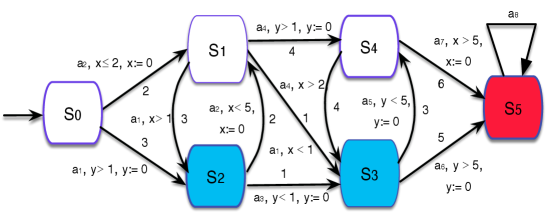
Figure 3: A WTA from [20] where states $s_{1},\,s_{3}$ and $s_{5}$ represent the goals of the attacker and the blue nodes satisfy $r_{s}$, the red node satisfies both $a$ and $r_{s}$, and the white ones satisfy neither $r_{s}$ nor $a$.

7 Implementation and Validation

We implemented a TOL verification algorithm within the VITAMIN model checker to validate our approach and assess its runtime performance. The VITAMIN tool is a prototype framework for modeling and verifying multi-agent systems, designed for both accessibility and extensibility: non-experts can use it effectively, while experts can modularly extend it with additional features [28]. To the best of our knowledge, VITAMIN is currently the only tool supporting OL and OATL, making it a natural choice for extending with real-time verification of TOL. Compared to mainstream model checkers such as MCMAS [46] and STV [41], implementing our algorithm in VITAMIN was more straightforward and better aligned with our objectives.

A brief description of the architecture is given to familiarize readers with the tool’s overall design and components, a more detailed description can be found in [28]. The main three modules depicted in Figure 4 are introduced below:

• Logics: Holds the parsers for each supported logic, at the time of writing 12 logics are supported.

• Models: Responsible for storing the code that parses input files and loads them into memory as a Concurrent Game Structure (CGS).

• Model checker/verifier: Is in control of verifying properties of models using the specified logic and model, there’s one for each supported logic.

Our contribution implied changes in all modules, and enabled the introduction of a (i) parsing of real-time formulas/constraints and (ii) real-time verification algorithm for TCGSs using backwards exploration of the generated zone graph, using the symbolic on-the-fly approach of Section 4.

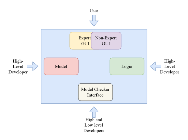
Figure 4: VITAMIN high-level architecture [29].

7.1 Experimental methodology

This section outlines the chosen methodology to validate the theoretical approach of the past sections. Our aim is to provide general runtime metrics of the verification algorithm with a number of selected case studies of varying size, the implementation in Python alongside the experimental data is available at: https://gitlab.telecom-paris.fr/david.cortes/vitamin.

We have crafted two models to serve as case studies, described in the following subsections. The first is the pipeline model, a simple sequence of $k$ nodes and $k$ edges forming a single path. Finally, we examine a strongly connected model of $k$ nodes, designed to showcase TOL’s ability to verify properties across paths, a capability inherited from CTL. A more comprehensive experimental evaluation is planned and will be added in a subsequent version.

Although, there are publicly available benchmarks for other real-time model checkers [1, 49], many of them are nearly a decade old. Additionally, many of the models or formulas are no longer available, and those that were available require substantial adaptions to be used in VITAMIN. As a result, even reproducing a baseline for our experiments proved difficult, which we see as a broader limitation in the field of real-time formal verification. Furthermore, our objective is not to compare VITAMIN with other more established and feature-rich tools, given that it is still a prototype direct comparisons at this stage wouldn’t be meaningful.

7.2 Case studies

Here, we detail each model and their TOL formulas used to generate the experimental data on VITAMIN.

Pipeline

The objective of this model is to test the performance of the real-time verification algorithm on simple models where there’s at most two possible transitions the attacker can take at any step (to wait, or take a discrete transition). Figure 5 shows a WTA for the instance where $k=4$.

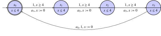
Figure 5: The pipeline model with $k=4$.

The TOL formula we will check against this model is

$$\varphi_{4}=j.\langle\textbf{\raisebox{2.22221pt}{\makebox[0.0pt][l]{\rule[-0.2pt]{3.33333pt}{0.4pt}}\makebox[3.33333pt]{\rule[-2.22221pt]{0.4pt}{6.66666pt}}}}_{1}\rangle\mathsf{G}\,(s_{3}\implies j\geq 16)$$

Which captures the objective: Anytime the attacker reaches $s_{3}$, at least 16 time units will have passed

And the more general formula is Anytime the attacker reaches $s_{n}$, at least $k*k$ time units will have passed:

$$\varphi=j.\langle\textbf{\raisebox{2.22221pt}{\makebox[0.0pt][l]{\rule[-0.2pt]{3.33333pt}{0.4pt}}\makebox[3.33333pt]{\rule[-2.22221pt]{0.4pt}{6.66666pt}}}}_{1}\rangle\mathsf{G}\,(s_{n}\implies j\geq k*k)$$

The reason we chose this formula is that we can force the algorithm’s worst case exploration with it, given that $s_{n}$ is the last location in the system, the backwards reachability algorithm starts on it, and then it will compute every time predecessor until the initial location is reached, effectively traversing most of the generated Zone Graph.

Mesh

Figure 6 shows the corresponding WTA for this model with $k=4$, where each node is reachable from every other node. The idea here is to collect runtime metrics that allows us to have a rough idea of how much resources could be consumed on large strongly connected graphs resembling the topology of mesh networks.

Figure 6: The strongly connected model with $k=4$.

We’re interested in running this model against the TOL formula:

$$\varphi=j.\langle\textbf{\raisebox{2.22221pt}{\makebox[0.0pt][l]{\rule[-0.2pt]{3.33333pt}{0.4pt}}\makebox[3.33333pt]{\rule[-2.22221pt]{0.4pt}{6.66666pt}}}}_{1}\rangle(s_{n}\land j\geq k*k)$$

Which means: There’s a strategy for the attacker where the last location ($s_{n}$) is reached in at least $k*k$ time units. There are multiple paths to $s_{n}$, but since we’re also requiring a minimum of time units, it will traverse a sizable chunk of the Zone Graph trying to find one instance that satisfies the property. We believe this will give us reasonable performance metrics for these kinds of graphs.

7.3 Preliminary evaluation

Our current prototype produces results on small to medium-scale instances, which we present here as initial validation. Therefore, the following data should be regarded as preliminary, with a complete benchmark evaluation deferred to a future update.

Experiments were run on an Apple M4 system with 16 GB of unified memory. For each case study, the model size was varied up to a maximum of 30.

Case study & input size	Runtime (ms)	Max memory (KB)
Pipeline $k=4$	$7.2\pm 0.8$	$25.63\pm 0.96$
Pipeline $k=12$	$13.2\pm 2.3$	$30.16\pm 1.04$
Pipeline $k=16$	$19\pm 6.6$	$34.24\pm 2.34$
Pipeline $k=22$	$21\pm 3.4$	$49.70\pm 0.74$
Pipeline $k=30$	$25.6\pm 5.3$	$77.89\pm 1.75$

Table 1: Obtained results with the pipeline model. We present the mean average runtime in milliseconds, and the mean peak allocated memory in kilobytes.

Case study & input size	Runtime (ms)	Max memory (KB)
Mesh $k=4$	$6.2\pm 1.3$	$26.27\pm 1.3$
Mesh $k=12$	$16.2\pm 3.9$	$43.42\pm 2.6$
Mesh $k=16$	$19.2\pm 4.1$	$67.11\pm 3.9$
Mesh $k=22$	$24.4\pm 2.4$	$112.86\pm 2.5$
Mesh $k=30$	$37.8\pm 3.4$	$196.65\pm 2.1$

Table 2: Obtained results with the mesh model. We present the mean average runtime in milliseconds, and the mean peak allocated memory in kilobytes.

We measured the average runtime and max allocated memory over five runs for every case study and input size, using Python’s tracemalloc and time modules. Then, the collected data were compiled into multiple CSV files and processed using Python notebooks. The aggregated results are shown in tables 1 and 2. Expectedly, we see the metrics increasing steadily with input size in both tables. The mesh model generally consumed more memory than the pipeline model, while keeping comparable execution times, except for the largest input size. The Python notebook along with the raw collected data is available at https://gitlab.telecom-paris.fr/david.cortes/vitamin-benchmarks.

7.4 Challenges and future work

Since VITAMIN is still in prototype phase, certain engineering aspects remain under development. This led to challenges such as build issues related to missing dependencies or unsupported versions, opening an avenue for exploring containerized solutions to streamline time to development. Additionally, automating the generation and collection of experimental data proved difficult given there’s no command-line access to the tool, we plan on working on this limitation next to support and provide much more comprehensive experimental analysis for an upcoming version of this paper.

We emphasize that these challenges are not fundamental obstacles but reflect the current prototype status. Addressing them will further strengthen the tool as it evolves into a stable and extensible platform.

8 Related Work

Lately, many papers have focused on the strategic capabilities of agents playing within dynamic game models. In this section, we compare our approach with some of these papers.

Untimed Games and Strategic Logics [58, 43, 8] some research related to sabotage games have been introduced by van Benthem with the aim of studying the computational complexity of a special class of graph reachability problems in which an agent has the ability to delete edges. To reason about sabotage games, van Benthem introduced Sabotage Modal Logic (SML). The model checking problem for the sabotage modal logic is PSPACE-complete [43]. Our version of the games is not comparable to the sabotage games, because we provide the possibility to temporarily select subsets of edges, while in the sabotage games the saboteur can only delete one edge at a time. In this respect, our work is related to [19], where the authors use an extended version of sabotage modal logic, called Subset Sabotage Modal Logic (SSML), which allows for the deactivation of certain subsets of edges of a directed graph. The authors show that the model checking problems for such logics are decidable. Furthermore, we recall that SSML is an extension of SML, but does not include temporal operators. Also, neither SML nor SSML takes into account quantitative information about the cost of edges, as we do. In [56] Dynamic Escape Games (DEG) have been introduced. A DEG is a variant of weighted two-player turn-based reachability games. In a DEG, an agent has the ability to inhibit edges. In [20] have been introduced an untimed Obstruction Logic (OL) which allows reasoning about two-player games played on a labeled and weighted directed graph. Thus, our TOL is an extension of OL. ATL [4] and SCTL [7] are extensions of CTL with the notion of strategic modality. These kinds of logics are used to express properties of agents as their possible actions. However, all these logics do not include quantitative information about costing edges, real-time and temporal operators.

Timed Games and Strategic Logics [33, 37, 25, 55, 7] several research works have focused on extending games and modal and temporal logics to the real-time domain. The most established model in this respect is the timed game automata [14, 25]. A Timed Game Automaton (TGA) is a TA whose set of transitions is divided among the different players. At each step, each player chooses one of her possible transitions, as well as some time she wants to wait before firing her chosen transition. The logics ATL and CTL has also been extended to TATL [33, 37] and STCTL [7], in which formula clocks are used to express the time requirements. It is exponentially decidable whether a TATL formula satisfies a TGA [33]. However, in [7] was shown that STCTL is more expressive than TATL and the model checking problem for STCTL with memoryless perfect information is of the same complexity as for TCTL. Model checking for TATL with continuous semantics is undecidable [7]. However, all these logics do not use dynamic models.

9 Conclusions

In this paper, we presented Timed Obstruction Logic (TOL), a logic that allows reasoning about two-player games with real-time goals, where one of the players has the power to locally and temporarily modify the timed game structure. We then proved that its model checking problem is PSPACE-complete. Furthermore, we showed how TOL expresses cybersecurity properties in a suitable way. There are several directions that we would like to explore for future work. A possible extension would be to consider timed games with many players, between a demon and coalitions of travelers. In our opinion, such an extension would have the same relationship with the TATL logic as TOL has with TCTL. Another extension could be to extend TOL with probability, since many cybersecurity case studies relate cyberattacks to the probability of success of the attack. Finally, another important line would be to introduce imperfect information in our setting. Unfortunately, this context is generally non-decidable [24]. In order to overcome this problem, we could use an approximation to perfect information [10], a notion of bounded memory [11], or some hybrid technique [26, 27].

References

- [1] UPPAAL benchmarks. https://archive.is/8fHwv. Accessed: 2025-10-01.
- [2] R. Alur, Techniques for Automatic Verification of Real-Time Systems, Ph.D. dissertation, Stanford University, (1991).
- [3] R. Alur and D. Dill, ‘A theory of timed automata’, Theoretical computer science, 126(2), 183–235, (1994).
- [4] R. Alur, T.A. Henzinger, and O. Kupferman, ‘Alternating-time temporal logic’, J. ACM, 49(5), 672–713, (2002).
- [5] R. Alur, S. La Torre, and G. J. Pappas, ‘Optimal paths in weighted timed automata’, in Computation and Control, pp. 49–62, (2001).
- [6] F. Alzetta, P. Giorgini, A. Najjar, M. I. Schumacher, and D. Calvaresi, ‘In-time explainability in multi-agent systems: Challenges, opportunities, and roadmap’, in Explainable, Transparent Autonomous Agents and Multi-Agent Systems, pp. 39–53, (2020).
- [7] J. Arias, W. Jamroga, W. Penczek, L. Petrucci, and T. Sidoruk. Strategic (timed) computation tree logic, (2023).
- [8] G. Aucher, J. Van Benthem, and D. Grossi, ‘Modal logics of sabotage revisited’, Journal of Logic and Computation, 28(2), 269 – 303, (2018).
- [9] G. Behrmann, A. David, and K. G. Larsen, ‘A tutorial on uppaal 4.0’, Department of computer science, Aalborg university, (2006).
- [10] F. Belardinelli, A. Ferrando, and V. Malvone, ‘An abstraction-refinement framework for verifying strategic properties in multi-agent systems with imperfect information’, Artif. Intell., 316, 103847, (2023).
- [11] F. Belardinelli, A. Lomuscio, V. Malvone, and E. Yu, ‘Approximating perfect recall when model checking strategic abilities: Theory and applications’, J. Artif. Intell. Res., 73, 897–932, (2022).
- [12] F. Belardinelli, V. Malvone, and A. Slimani. A tool for verifying strategic properties in mas with imperfect information, 2020.
- [13] J. Bengtsson and W. Yi, ‘Timed automata: Semantics, algorithms and tools’, in Lectures on Concurrency and Petri Nets, Lecture Notes in Computer Science, 87–124, (2004).
- [14] P. Bouyer, U. Fahrenberg, K. G. Larsen, and N. Markey, ‘Quantitative analysis of real-time systems using priced timed automata’, Communications of the ACM, (2011).
- [15] M. Bozga, C. Daws, O. Maler, A. Olivero, S. Tripakis, and S. Yovine, ‘Kronos: A model-checking tool for real-time systems’, in Computer Aided Verification: 10th International Conference, CAV’98, (1998).
- [16] D. Calvaresi, Y. Dicente Cid, M. Marinoni, A. F. Dragoni, A. Najjar, and M. I. Schumacher, ‘Real-time multi-agent systems: rationality, formal model, and empirical results’, Autonomous Agents and Multi-Agent Systems, 35, (2021).
- [17] D. Calvaresi, M. Marinoni, A.Sturm, M. I. Schumacher, and G. C. Buttazzo, ‘The challenge of real-time multi-agent systems for enabling iot and cps’, Proceedings of the International Conference on Web Intelligence, (2017).
- [18] D. Catta, J. Leneutre, and V. Malvone, ‘Subset sabotage games & attack graphs’, in Proceedings of the 23rd Workshop "From Objects to Agents", volume 3261, pp. 209–218. CEUR-WS.org, (2022).
- [19] D. Catta, J. Leneutre, and V. Malvone, ‘Attack graphs & subset sabotage games’, Intelligenza Artificiale, 17(1), 77–88, (2023).
- [20] D. Catta, J. Leneutre, and V. Malvone, ‘Obstruction logic: A strategic temporal logic to reason about dynamic game models’, in ECAI 2023 - 26th European Conference on Artificial Intelligence, (2023).
- [21] J. Cho, D. Sharma, H. Alavizadeh, S. Yoon, Noam B-A., T. Moore, Dan Kim, H. Lim, and F. Nelson, ‘Toward proactive, adaptive defense: A survey on moving target defense’, IEEE Communications Surveys & Tutorials, (2020).
- [22] E. M. Clarke, O. Grumberg, and D. A. Peled, Model Checking, The MIT Press, Cambridge, Massachusetts, (1999).
- [23] E.M. Clarke and E.A. Emerson, ‘Design and Synthesis of Synchronization Skeletons Using Branching-Time Temporal Logic.’, (1981).
- [24] C. Dima and F. L. Tiplea, ‘Model-checking ATL under imperfect information and perfect recall semantics is undecidable’, CoRR, (2011).
- [25] M. Faella, S. La Torre, and A. Murano, ‘Automata-theoretic decision of timed games’, Theor. Comput. Sci., 515, 46–63, (2014).
- [26] A. Ferrando and V. Malvone, ‘Towards the combination of model checking and runtime verification on multi-agent systems’, in 20th International Conference, PAAMS 2022, (2022).
- [27] A. Ferrando and V. Malvone, ‘Towards the verification of strategic properties in multi-agent systems with imperfect information’, in Proceedings of the 2023 International Conference on Autonomous Agents and Multiagent Systems, AAMAS 2023, (2023).
- [28] Angelo Ferrando and Vadim Malvone. Vitamin: A compositional framework for model checking of multi-agent systems, 2025.
- [29] Angelo Ferrando and Vadim Malvone. VITAMIN: A Compositional Framework for Model Checking of Multi-Agent Systems, March 2025.
- [30] T. A Henzinger, P-H. Ho, and H. Wong-Toi, ‘Hytech: A model checker for hybrid systems’, in Computer Aided Verification: 9th International Conference, CAV’97, (1997).
- [31] T. A. Henzinger, Z. Manna, and A. Pnueli, ‘Timed transition systems’, in Real-Time: Theory in Practice, (1992).
- [32] T. A. Henzinger, X. Nicollin, J. Sifakis, and S. Yovine, ‘Symbolic model checking for real-time systems’, Technical report, USA, (1994).
- [33] T. A. Henzinger and V. S. Prabhu, ‘Timed alternating-time temporal logic’, in 4th International Conferences on Formal Modelling and Analysis of Timed Systems (FORMATS’06), (2006).
- [34] W. Jamroga and A. Murano, ‘Module checking of strategic ability’, in AAMAS 2015, (2015).
- [35] N. R. Jennings and M. Wooldridge, ‘Application of intelligent agents’, in Agent Technology: Foundations, Applications, and Markets, (1998).
- [36] K. Kaynar, ‘A taxonomy for attack graph generation and usage in network security’, J. Inf. Secur. Appl., 29(C), 27–56, (2016).
- [37] M. Knapik, É. André, L. Petrucci, W. Jamroga, and W. Penczek, ‘Timed ATL: forget memory, just count’, J. Artif. Intell. Res., (2019).
- [38] O. Kupferman, U. Sattler, and M. Y. Vardi, ‘The complexity of the graded -calculus’, in Automated Deduction - CADE-18, 18th International Conference on Automated Deduction 2002, (2002).
- [39] O. Kupferman, M.Y. Vardi, and P. Wolper, ‘An Automata Theoretic Approach to Branching-Time ModelChecking.’, Journal of the ACM, (2000).
- [40] O. Kupferman, M.Y. Vardi, and P. Wolper, ‘Module Checking.’, Information and Computation, 164(2), 322–344, (2001).
- [41] Damian Kurpiewski, Wojciech Jamroga, and Michał Knapik, ‘Stv: Model checking for strategies under imperfect information’, in Proceedings of the 18th International Conference on Autonomous Agents and MultiAgent Systems, AAMAS ’19, p. 2372–2374, Richland, SC, (2019). International Foundation for Autonomous Agents and Multiagent Systems.
- [42] F. Laroussinie, N. Markey, and G. Oreiby, ‘Model-checking timed atl for durational concurrent game structures’, in Formal Modeling and Analysis of Timed Systems, 4th International Conference, FORMATS 2006, (2006).
- [43] C. Löding and P. Rohde, ‘Model checking and satisfiability for sabotage modal logic’, in FST TCS 2003: Foundations of Software Technology and Theoretical Computer Science, (2003).
- [44] A. Lomuscio, H. Qu, and F. Raimondi, ‘MCMAS: A model checker for the verification of multi-agent systems’, in Proceedings of the 21th International Conference on Computer Aided Verification (CAV09), (2009).
- [45] A. Lomuscio, B. Woźna, and A. Zbrzezny, ‘Bounded model checking real-time multi-agent systems with clock differences: Theory and implementation’, in Model Checking and Artificial Intelligence, (2007).
- [46] Alessio Lomuscio, Hongyang Qu, and Franco Raimondi, ‘Mcmas: an open-source model checker for the verification of multi-agent systems’, International Journal on Software Tools for Technology Transfer, 19(1), 9–30, (2017).
- [47] Hector Marco-Gisbert and Ismael Ripoll Ripoll, ‘Address space layout randomization next generation’, Applied Sciences, 9(14), (2019).
- [48] F. Mogavero, A. Murano, G. Perelli, and M. Y. Vardi, ‘Reasoning about strategies: On the model-checking problem’, ACM Transactions in Computational Logic, (2014).
- [49] Georges Morbé and Christoph Scholl, ‘Fully symbolic tctl model checking for complete and incomplete real-time systems’, Science of Computer Programming, 111, 248–276, (2015).
- [50] A. Murano, G. Perelli, and S. Rubin, ‘Multi-agent path planning in known dynamic environments’, in PRIMA 2015: Principles and Practice of Multi-Agent Systems - 18th International Conference, (2015).
- [51] N. Nguyen and A. Rakib, ‘Formal modelling and verification of probabilistic resource bounded agents’, Journal of Logic, Language and Information, (2023).
- [52] J. Ortiz, M. Amrani, and P. Y. Schobbens, ‘Mlv: A distributed real-time modal logic’, in NASA Formal Methods - 11th International Symposium, NFM 2019, Proceedings, Germany, (2019).
- [53] G. D. Plotkin, ‘A structural approach to operational semantics’, Technical Report DAIMI FN-19, University of Aarhus, (1981).
- [54] A. Qasim, I. Fakhir, and S. Kazmi, ‘Formal specification and verification of real-time multi-agent systems using timed-arc petri nets’, Advances in Electrical and Computer Engineering, (2015).
- [55] A. Qasim, S. Kanwal, A. Khalid, R. Kazmi S. Asad, and J. Hassan, ‘Timed-arc petri-nets based agent communication for real-time multi-agent systems’, International Journal of Advanced Computer Science and Applications, (2019).
- [56] A. Di Stasio, P. D. Lambiase, V. Malvone, and A. Murano, ‘Dynamic escape game’, in Proceedings of the 17th International Conference on Autonomous Agents and MultiAgent Systems, AAMAS 2018, (2018).
- [57] Stavros Tripakis and Sergio Yovine, ‘Analysis of timed systems using time-abstracting bisimulations’, In Formal Methods in System Design, 25–68, (2001).
- [58] J. van Benthem, An Essay on Sabotage and Obstruction, Springer Berlin Heidelberg, 2005.