Dynamic breaking of axial symmetry of acoustic waves in crystals as the origin of nonlinear inelasticity and chaos: Analytical model and MD simulations.

Abstract

A Chain of Springs and Masses (CSM) model is used in the interpretation of molecular dynamics (MD) simulations of movement of atoms in FCC crystals, oriented like during typical simulations performed in studies of the dynamics of line dislocations. The proposed description is inspired by and supported by MD simulations. We find out that a force that is perpendicular to the direction of the applied external shear pressure and in the direction of line dislocations occurs within the bulk of crystal volume. The force is of a dynamic origin, and it has not been analyzed so far. It is proportional to the square of the applied pressure; It causes breaking of axial symmetry for propagation of transverse acoustic waves. It leads to a non-linear and non-elastic response of crystals and to chaotic patterns in motion of atoms. We provide an analytical derivation of an effective atomistic potential for interaction between atoms and propose an analytical model of their dynamics. The model predicts some effects that may have been overlooked in experiments and are inconsistent with the static theory of elasticity of crystals.

Keywords: Molecular dynamics simulations, Chain of springs and masses, Elastic properties, Pressure propagation, Nonlinear, Chaos

1 Introduction.

1.1 The model of a Chain of Springs and Masses (CSM).

The CSM model, based on the works of Schrödinger (1914) [1, 2], and Pater (1974)[3], has been found recently [4] suitable as an analytical description of the dynamics of layers in oriented FCC crystals studied by the Molecular Dynamics (MD) technique. On the side of MD simulations, the method is to determine time-evolution of averages of some physical quantities when an external pressure is applied to the outer surface of the sample. These quantities are, for instance, $\langle X_{i,n}\rangle$, $\langle V_{i,n}\rangle$ (displacement and velocity of atoms, respectively, in arbitrary direction $i$). $\langle\rangle$ means an average over all atoms within the plane, while index n enumerates planes, starting with n = 1 for the surface rigid plane, where force is applied, and with n = N for the plane with the lowest Y value, which is fixed (planes are perpendicular to the Y-direction, which is the [111] crystallographic direction, while external force is applied in the X-direction [1$\bar{1}$0], and the Z-axis is along [$\bar{1}$$\bar{1}$2]). That geometry is typical in simulations where studies of the dynamics of dislocations are performed in FCC crystals [5]. The symmetry conditions imposed in the lammps simulation tool [6] are written as psp, which means that atoms can move and interact with any atoms through the simulation box boundary in directions X and Z, but not in direction Y. This is apparently the main reason why a collection of atoms behaves like it was forming a chain of layers (with nearly rigidly connected atoms within each layer), while layers interact effectively through a spring between them. The other reason is that atoms are coupled stronger within layers than between layers due to difference of distance between them in corresponding directions. There is evidence of the validity of the CSM model based on numerous simulations, of which a part only has been published[4] by us so far.

The model predicts some surprising, mathematically rich features. For instance, the sound speed is found dependent on the time/distance of the wave traveled, and it depends also on how the threshold value of the sound wave is defined in any experiments. That is caused by a change of sound wave profile with time/distance. Oscillations in quantities like velocity or forces were found, and their frequency changes with time. Amplitudes of oscillations have a time-dependence close to power-law or a stretched-exponetial function of time.

1.2 The motivation.

It follows from elementary symmetry considerations that Cauchy forces in the Z-direction (and in the Y-direction as well) ought to be equal to zero when a static shear pressure is applied in the X-direction at the surface. That implies also the absence of any movement of atoms (layers) in the Z-direction.

However, in our simulations (which are, obviously, carried out in a dynamic way) we observe notoriously that some small forces (a few orders of magnitude smaller than forces in the X-direction) are observed. These forces are proportional to the square of the applied pressure in the X-direction, and, therefore, they diminish quickly when the pressure value is very small.

Moreover, we are able to determine the dynamics in the Z-direction, finding out that there is no exact agreement between forces and acceleration as it ought to follow from Newtonian mechanics. However, if a small contribution to forces in Z is added from forces in X-, such an agreement could be obtained. In other words, we observe a mixing of X- and Z-components of forces (movement), which contradicts the common belief of what ought to be observed in a case of angularely isotropic potential.

The initial aim of this work was to gain an understanding of the mechanisms behind the occurrence of frequency beats in oscillations observed at large pressures applied, in quantities like velocity of layers, or force acting on them, as reported first in [4]; see figure 6 there. However, we will not discuss here these frequency beats, even though we already have a reliably good knowledge on that, leaving the subject for another article. Instead, we will concentrate on describing how an unusual force component contributes to the dynamics of stress of crystals. Actually, that force component - to the best of our knlowledge, not discussed in any papers so far - is the cause of precession in 2D phase space, leading to frequency beats.

1.3 Samples, potentials and simulation setup.

We use as simple as possible crystallographic structure and interatomic interaction potential that allows us to reproduce the most basic dynamical mechanisms similar to those in real systems, where line dislocation movement is observed, i.e., in an oriented FCC lattice. Therefore, we use a harmonic interaction between atoms and a perfectly ordered monoatomic crystal. The details of sample preparation, geometric configuration, creating the interatomic potential, MD simulations, and the data analysis methods have been described previously [7, 4].

This time we use the lepton interatomic potential available in lammps, alongside the previously used by us the table style potential of our design [8] - in experiments described here, both potentials lead to identical results.

A proper statistical averaging of physical quantities along the X direction, for every layer of atoms in the Y-direction is one of the most important steps in the data analysis, and it is probably causing the largest difficulty to other researches attempting to repeat similar simulations. Some related technical details are given in [9].

In simulations of the long-time dynamics of the CSM model, we use a harmonic inter-atomic potential $E_{p}(r)=\epsilon_{0}\cdot(r-r_{0})^{2}$, with the parameter $\epsilon_{0}$ = 1 eV/Ų, where $r$ is the distance between atoms, $r_{0}=a/\sqrt{2}$, and $a$ is the FCC lattice constant, the same as in steel, $a$ = 3.56 Å, with the mass of atoms assumed as that of Fe.

Results reported in [4] were obtained, mostly, on a sample with 8 atoms in one layer. We, however, realized (and checked carefully) that only two atoms in a layer are sufficient for carrying out most of MD simulations described here (that speeds up the simulation time, data analysis time, and decreases the amount of stored data). There are some exceptions to that when it was necessary to use larger sample sizes. Here, the sample has N=1500 layers in the Y-direction (the length is over 0.3 $\mu$m).

The results of simulations are, usually, very accurate, exceeding 5-6 significant digits.

1.4 The plan of this article.

In section 2 we compare how the time dependencies of some physical quantities (displacement, velocity, force) differ for directions X and Z, when the free movement of layers/particles/atoms in the Z-direction is enabled. We show there some phase-space diagrams, bringing some light on the possible mechanisms behind the interaction between particles.

In section 3, which is crucial, we derive exact equations on the interlayer potential depending on coordinates x and z, we show that it has the main harmonic contribution that is axially symmetric and a small contribution that grows up as a third power of distance from its minimum and has a threefold axial symmetry. We provide evidence based on MD simulation results of, e.g., angular dependence of forces, that the simulations are in agreement with the derived potential energy. We also propose approximate equations of motion of a particle and show how the dynamics of the system becomes chaotic.

In discussion section 4 we point out how the proposed description relates to the Christoffel equations that describe atomic motions by using a plane-wave formalism, and attempt to formulate how to solve the problem of the motion of waves in the bulk of material by using a pair of nonlinear coupled difference equations. Possible experimental consequences of the model are mentioned as well.

2 Comparison of dynamics in X- and Z-directions.

2.1 The linear case, with no movement in Z-direction.

At low values of the applied surface pressure, let’s say below 10 MPa, the results of MD simulations can be described exactly by solutions of a 1-dimensional CSM model, as shown in [4]. Hence, after an abrupt pressure is applied at the surface (Heaviside mode of simulations) the time dependend quantities like the displacement of layers, ${u}_{n}^{H}$, their velocity ${v}_{n}^{H}$ and the force acting on them, ${f}_{n}^{H}$, has the form:

$${u}_{n}^{H}=\frac{{F}_{1}}{{\rm{m}}{{\rm{\Omega}}}^{2}}\cdot\left[{J}_{2n}(2\theta)+\displaystyle\sum_{k=2n+2,2n+4,...}^{\infty}(k-2n+1){J}_{k}(2\theta)\right],$$ (1)

$${v}_{n}^{H}=\frac{{F}_{1}}{{\rm{m}}{\rm{\Omega}}}\cdot\left[{J}_{2n-1}(2\theta)+2\cdot\displaystyle\sum_{k=2n+1,2n+3,...}^{\infty}{J}_{k}(2\theta)\right],$$ (2)

$${f}_{n}^{H}=-{F}_{1}\cdot\left[{J}_{2n}(2\theta)+2\cdot\displaystyle\sum_{k=2n+2,2n+4,...}^{\infty}{J}_{k}(2\theta)\right],$$ (3)

where $J_{n}$ are Bessel functions of the first kind and $\theta=\Omega t$, m is the mass of a particle/layer, and $F_{1}$ is the force exerted on the uppermost layer. The parameter $\Omega$ used there is the fundamental angular frequency of oscillations of two layers: it can be determined by using several methods from MD simulations, and it is in agreement with the value computed from first principles[4]. The superscript ^H refers to the Heaviside method of simulations.

A very similar, numerically nearly identical one, is a solution for an often-used case when a constant rate of the surface-applied strain is used in MD simulations. Let us list these equations as well, for a reference (the superscript ^V is used to distinguish the case from the Heaviside mode of simulations):

$$u^{V}_{n}(t)=\frac{v_{0}}{\Omega}\left[J_{2n-1}(2\theta)+\sum_{k=2n+1,2n+3,...}^{\infty}(k-2n+2)J_{k}(2\theta)\right],$$ (4)

$$v^{V}_{n}(t)=v_{0}\left[J_{2n-2}(2\theta)+2\cdot\sum_{k=2n,2n+2,...}^{\infty}J_{k}(2\theta)\right],$$ (5)

$$f^{V}_{n}(t)=-mv_{0}\Omega\cdot\left[J_{2n-1}(2\theta)+2\cdot\sum_{k=2n+1,2n+3,...}^{\infty}J_{k}(2\theta)\right].$$ (6)

In 4-6, $v_{0}$ is the imposed constant velocity of the surface layer. These equations have been deduced from accurate analysis of results of MD simulations. In the constant surface velocity method (which is equivalent to the constant surface strain rate $\dot{\epsilon}=v_{0}/d$, where $d$ is the sample size in the direction of the applied force), the equations are related to these in the Heaviside method, with velocity $v_{0}$ in 5 having the same value as the prefactor in 2, with the force at the surface, $F_{1}$, creating the same pressure values in the sample volume of the constant velocity mode.

In the linear case, as given by 1-3, simulations do not show, obviously, any observable contribution to quantities in Z-direction, i.e., in the displacement, velocity, or force, $\Delta Z$, $V_{Z}$ or $F_{Z}$.

The linear case is realized in simulations by two methods: 1) when the applied pressure is very low, the system response may be considered linear as a function of pressure, or 2) when a condition is imposed in lammps that forces do not act on atoms in the Z-direction, by a command like this:
fix id all setforce NULL 0 0.

In the first method any response scales up linearly with the applied pressure. The pressure range where this is valid is up to around 10 MPa (which is a somewhat arbitrary value, depending on the desired accuracy). In case 2) the linear response is preserved up to around 10 GPa (i.e., up to the largest pressure values we can apply).

2.2 The nonlinear case, with movement in the Z-direction allowed.

Figures 1-3 show a comparison of some physical quantities in directions X and Z when atoms are free to move in the X and Z directions, and the system is in the nonlinear regime after we use
fix id all setforce NULL 0 NULL.

At a pressure of 100 MPa, as in figures 1-3, the X quantities are still responding nearly linearly to pressure, while Z quantities are small but already well visible in simulations and scale up as the second power of pressure. Notice the difference in vertical scales between a) and b) in figures 1-3.

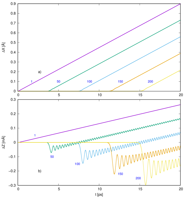
Figure 1: Comparison of average displacement of layers in the X-direction (figure a) and in the Z-direction (b), when the shear pressure of 100 MPa is applied at the surface in the X-direction. Labels indicate the number of layer.

The slope dX/dt (after the pressure wave reached the layer) is 0.04502 Å/ps. It is an average velocity of layers in the X-direction, $V_{X}$. When performing simulations with disabled movement in the Z-direction, that velocity is proportional to the applied pressure, with a high accuracy, from the lowest pressure values investigated (of the order of 10^-3 MPa) up to around 8 GPa: $V_{X}=0.0004502\cdot P$ Å/ps, where P is in MPa. The proportionality coefficient is in perfect agreement with the value computed by using the CSM model [4].

It was unexpected to observe, as in figure 1 b), that a displacement in the Z-direction is present as well. Moreover, when simulations are done by applying force in the opposite direction (still, along the X-axis) we observe an increase of Z(t) as well, following exactly the same curves, showing that the sign of the displacement Z(t) does not depend on the sign of the applied force. Additionally, we could compensate Z(t) to zero value by adding in simulations a very small force component in the Z-direction.

The slope of dZ/dt =0.001323 Å/ps in b) is the same for all layers.

dZ/dt is the average velocity of layers in Z-direction, $V_{Z}$. That velocity has a different dependence on the applied pressure than $V_{X}$. With a high accuracy, it can be approximated by a parabolic function of pressure, $V_{Z}\sim P^{2}$.

The sign of velocity $V_{X}$ depends on the sign of the applied pressure.

In the case of $V_{X}$ in 2 a), we can see clearly that at long times velocity oscillates around certain equilibrium value; we name it $V_{x0}$. This is also observed in the case of $V_{Z}$ in 2 b), when at assymptotically long time, a value $V_{z0}$ is reached, though that value is small and it can not be seen in the scale of the figure b).

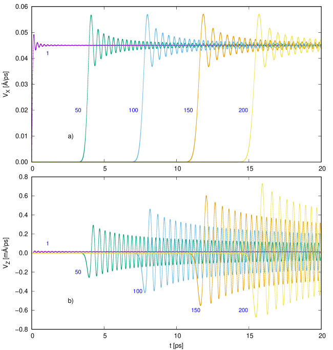
Figure 2: Comparison of average velocity of layers in the X- and Z-directions, $V_{X}$ and $V_{Z}$, under the same simulation conditions and for the same layers as in figure 1. Velocities are time derivatives of displacement curves shown in figure 1.

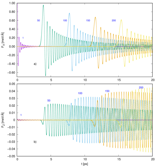
Figure 3: Comparison of average forces acting on layers in the X- and Z-directions, under the same simulation conditions and for the same layers as in figures 1 and 2. Notice the difference in vertical scale in a) and b).

2.3 Some phase-space diagrams.

Before drawing some hypothesis about the mechanisms behind the observed dependencies, let us analyze a few phase-space diagrams.

In figure 4 the dependence of $V_{z}(V_{x})$ is shown, where both quantities are normalized by their respective values at asymptotically long times, i.e., by $V_{z0}$ and $V_{x0}$. As we see, the layer 1 moves initially, at short times along the direction of the applied force, while the movement of layer 2 deviates strongly from the direction of surface force right from t=0. These results suggest that there is some difference between the dynamic behavior of the first and the next layers.

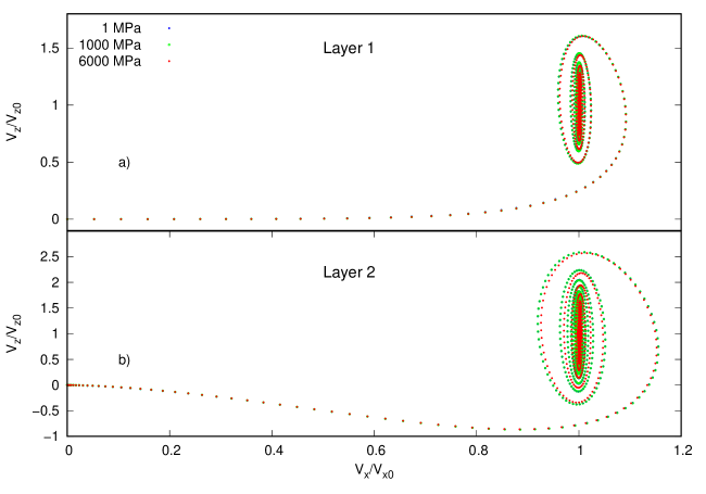
Figure 4: Phase-space portrait of $V_{z}(V_{x})$ for three values of pressure, as shown in the legend, when pressure is applied at an angle $0\mathrm{°}$ with respect to the X-axis. a) shows dependencies for layer 1 and b) for layer 2). $V_{x0}$ scales up linearly with pressure; therefore, its value changes here by 6000 times, while $V_{z0}$ changes as $P^{2}$, hence it changes here $36\cdot 10^{6}$ times.

The results shown so far suggest the existence of a force in the Z-direction when the surface force is applied in the X-direction. Hence, we conclude that in general, the results may depend on the direction of the applied force. Therefore, we carried out simulations for different angles $\alpha$ of the applied force with respect to the X-axis. This is done by defining in lammps the force (pressure) components by a command like this:
fix id upper aveforce Fx 0 Fz,
where $Fx=F1\cdot\cos(\alpha)$ and $Fz=F1\cdot\sin(\alpha)$ for a force of amplitude $F1$. Figure 5 shows the results for $V_{z}(V_{x})$ for several angles $\alpha$ when the pressure has a value of 1000 MPa, and also for 2000, 3000 and 4000 MPa when $\alpha=$$$. We would expect that these curves are simply straight lines at the same angles with respect to the X-axis as the applied external force. However, this is not the case. Only for angles of $30\mathrm{°}$ $\pm$ integer multiples of $60\mathrm{°}$ the dependence $V_{z}(V_{x})$ is linear. In the limit of long times, well-defined values of velocities for $V_{x}$ and $V_{z}$ are observed, $V_{x0}$ and $V_{z0}$, respectively. These are marked, for the angle $0\mathrm{°}$, by black dots on green curve given by a parabolic function. A linear dependence on pressure is observed, $V_{x0}=4.502\penalty 10000\ 10^{-4}\cdot P$, where P is in MPa and $V_{x0}$ is in Å/ps. That dependence is well understood, and it follows from exact analytical solutions of equations of motion, as described in [4]. For $V_{z0}(P)$ the dependence is of a parabolic type: $V_{z0}=1.29\penalty 10000\ 10^{-9}\cdot P^{2}$. Hence, that results in the observed dependence $V_{z0}=0.00637\cdot V_{x0}^{2}$, as shown by the green line.

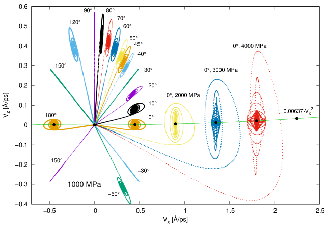
Figure 5: Phase space dependencies $V_{z}(V_{x})$ for layer 50 (time is a hidden parameter there). For pressure of 1000 MPa a number of curves is shown for a set of angle values, where angles are the direction of the applied pressure at the surface. For pressure applied at an angle of $0\mathrm{°}$ with respect to the X-axis, there are also curves drawn for 2000, 3000 and 4000 MPa.

3 On the origin of Z-forces.

3.1 The interlayer potential.

The insets of figure 6, a) and b), show the arrangement of atoms in layers 1,2, and 3, where layer 1 is the one where force is applied. That arrangement is shown for two different orientations. Colors of atoms in a) are the same as in b): The uppermost layer 1 is colored in red, the second layer is in green (only one atom shown in a) in that case), and the lowest layer is in blue. Hence, in a) the green atom has 3 NN atoms in the upper layer in red and 3 NN atoms in the lower layer in blue.

In [4], when computing the potential energy change due to a displacement of the green atom in the X-direction, we assumed that the arrangement of atoms in the upper and lower layers (red and blue, respectively) does not change. In that case an isotropic potential in the XZ plane is obtained.

However, in our dynamic simulations the wave of stress propagates along the Y-direction. That leads first to a displacement in the X-direction of the upper layer and next of the lower layer. In other words, there is some time difference between the displacement of layers 1 and 3. That causes a difference, at any instant of time, between forces acting on layer 2 from the side of layers 1 and 3.

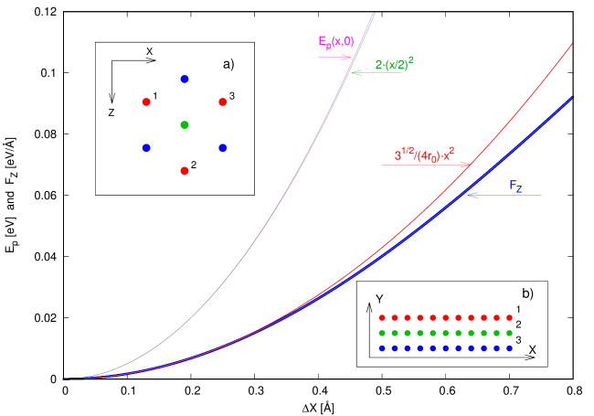
Figure 6: Potential energy $E_{p}$ and force component $F_{z}$ for one layer have been determined from MD simulations when the upper layer 1 is moved in the X-direction (no NVE integration is performed, while layers 2 and 3 have a force equal 0 imposed in all 3 directions (hence, these layers do not move). $E_{p}(x,0)$ (magenta curve) is the potential energy $E_{p}(x,z)$ computed by using Eq. 10, when z=0. The green curve shows its approximation at low x-values by a parabolic dependence. Densely packed blue dots show an $F_{Z}$ component of force, as determined from simulations, with the red curve being its approximation by a parabolic dependence, while the tiny yellow line drawn on top of blue data points is the computed exact analytical function based on 10. Inset boxes a) and b) show schematic arrangements of atoms during simulations, as described in the main text.

Let us first discuss equations on the potential energy when a displacement in x and z is taken into account, in a full analogy to what is done in [4], before proceeding to next simulation experiments.

The distance between the green atom in 6 a) and the 3 nearest neighbor (red) atoms on the next plane can be written as

$$r_{1}\left(x,z\right)=r_{0}\cdot\sqrt{1-\frac{x}{r_{0}}+\left(\frac{x}{r_{0}}\right)^{2}-\frac{z}{\sqrt{3}r_{0}}+\left(\frac{z}{r_{0}}\right)^{2}},$$ (7)

$$r_{2}\left(x,z\right)=r_{0}\cdot\sqrt{1+\left(\frac{x}{r_{0}}\right)^{2}+\frac{2z}{\sqrt{3}r_{0}}+\left(\frac{z}{r_{0}}\right)^{2}},$$ (8)

$$r_{3}\left(x,z\right)=r_{0}\cdot\sqrt{1+\frac{x}{r_{0}}+\left(\frac{x}{r_{0}}\right)^{2}-\frac{z}{\sqrt{3}r_{0}}+\left(\frac{z}{r_{0}}\right)^{2}}.$$ (9)

The subscripts in $r_{1}$,$r_{2}$,$r_{3}$ refer to labels of atoms in 6 a).

The potential energy $E_{p}(x,z)$ of the green atom can be written therefore as

$$E_{p}(x,z)=\epsilon_{0}\left[\left(r_{1}(x,z)-r_{0}\right)^{2}+\left(r_{2}(x,z)-r_{0}\right)^{2}+\left(r_{3}(x,z)-r_{0}\right)^{2}\right].$$ (10)

One can show, similarly as done in [4], that to the lowest order of x,z, the potential as given by Eq. 10 is isotropic, and it can be approximated by:

$$E_{p}\left(x,z\right)\approx 2\epsilon_{0}\cdot\left(\left(\frac{x}{2}\right)^{2}+\left(\frac{z}{2}\right)^{2}\right).$$ (11)

We used equation 10 to compute the contours of iso-potential curves, as shown in 7 and 8.

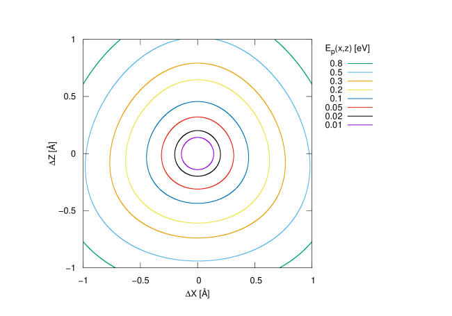
Figure 7: Iso-potential energy countors computed by using Eq. 10.

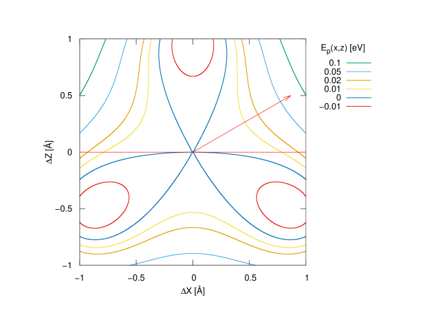
Figure 8: Iso-potential energy contours computed by using Eq. 10, with subtracted isotropic contribution, as given by 11. Hence, what is shown is the contribution breaking the axial symmetry around the point x=z=0. The arrow has an angle of $30\mathrm{°}$ with respect to the X axis.

Now, we are interested in computing forces based on derivatives of potential in the Z-direction:

$$\frac{\partial E_{p}(x,z)}{r_{0}\epsilon_{0}\partial z}=\left(1-\frac{r_{0}}{r_{1}}\right)\cdot\left(\frac{-1}{\sqrt{3}}+\frac{2z}{r_{0}}\right)+\left(1-\frac{r_{0}}{r_{2}}\right)\cdot\left(\frac{2}{\sqrt{3}}+\frac{2z}{r_{0}}\right)+\left(1-\frac{r_{0}}{r_{3}}\right)\cdot\left(\frac{-1}{\sqrt{3}}+\frac{2z}{r_{0}}\right)$$ (12)

A full exact analytical expression on $\partial E(x,z)/\partial z$ appears to be a complex one. For our needs, in the case of z=0, i.e., for computing force in the Z-direction when pressure is applied along the X-direction, it is sufficient to use a Taylor expansion of 12, with only two terms (in units of eV/Å):

$$\frac{\partial E_{p}(x,z)}{\partial z}\Big|_{z=0}\approx\epsilon_{0}/r_{0}\cdot\left(\sqrt{3}/4\cdot x^{2}-85/192\cdot x^{4}/r_{0}^{2})\right).$$ (13)

The parabolic term in 13 has a curvature $\epsilon_{0}\sqrt{3}/(4r_{0})=0.1720$ eV/ų, in agreement with the force determined in simulations (a derivative computed numerically by using 12 is in a perfect agreement with simulated results as well, up to x=0.8 Å, as shown in 6).

We notice that 13 does not depend on a sign of x.

For an analysis of the angle dependence of equation 10, we need to transform it to cylindrical coordinates. This is done by replacing quantities $x$ and $z$ by $r\cdot\cos\alpha$ and $r\cdot\sin\alpha$, respectively. In that case a dependence on $r$ and $\alpha$ is obtained, where $r=(x^{2}+z^{2})^{1/2}$. We obtain the following on the force $F_{\alpha}$ that is perpendicular to the direction $\hat{r}$, i.e., in the direction $\hat{\alpha}$:

$$F_{\alpha}=\frac{1}{r}\frac{\partial E_{p}(r,\alpha)}{\partial\alpha}.$$ (14)

After some basic (though lengthy) algebraic manipulations, 14 can be written in the form:

$$\frac{F_{\alpha}(r,\alpha)}{r_{0}\epsilon_{0}}=\left(\frac{r_{0}}{r_{3}}-\frac{r_{0}}{r_{1}}\right)\cdot\sin\alpha+\left(\frac{r_{0}}{r_{1}}-\frac{2r_{0}}{r_{2}}+\frac{r_{0}}{r_{3}}\right)\cdot\frac{\cos\alpha}{\sqrt{3}}.$$ (15)

One can check that under rotation for $60\mathrm{°}$, 15 changes as follows: $F_{\alpha}(r,\alpha+$$)=-F_{\alpha}(r,\alpha)$ (indexes in $r$ must be rotated as well: 1 $\rightarrow$ 2, 2 $\rightarrow$ 3, 3 $\rightarrow$ 1). Therefore, we must have also: $F_{\alpha}(r,\alpha+$$)=F_{\alpha}(r,\alpha)$, which proves the three-fold rotational symmetry of the potential.

3.2 Angular dependence of forces.

Figure 6 shows the dependence of $F_{Z}$ on a displacement in the X-direction, i.e., when the displacement direction has an angle of $0\mathrm{°}$ with respect to the X-axis. In order to investigate the angular dependence of potential and forces, we performed similar simulations for an arbitrary angle of the displacement with respect to the X-axis.

For that, we registered average forces $F_{X}$ and $F_{Z}$ as a function of the displacement distance $r$, for a large number of angles $\alpha$. In these cases, the displacement vector is given by $\vec{r}=r\cdot\hat{r}$, where $\hat{r}$ is a unit vector, $\hat{r}=(\cos\alpha,\sin\alpha)$. The aim was to find out a force in the direction $\hat{\alpha}$, which is perpendicular to $\hat{r}$. From the condition or orthogonality between these unit vectors, $\hat{r}\cdot\hat{\alpha}=0$, we find out that $\hat{\alpha}$ is defined as: $\hat{\alpha}=(-\sin\alpha,\cos\alpha)$. Therefore, when force F is given as $\vec{F}=(F_{X},F_{Z})$, the force acting in the $\hat{\alpha}$ direction must be given by

$$F_{\alpha}=\hat{\alpha}\cdot\vec{F}=-\sin\alpha\cdot F_{X}+\cos\alpha\cdot F_{Z}.$$ (16)

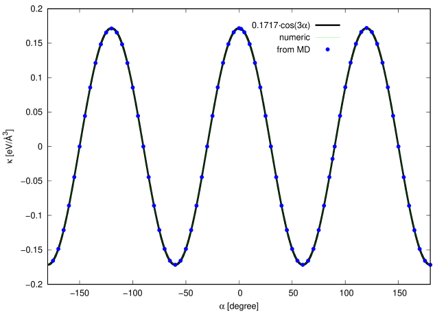
Figure 9: Angular dependence of $\kappa$. Blue dots labeled as "from MD" have been obtained by fitting parabolic dependence to $F_{\alpha}(r)$, as described in the text. These data are very well described by a function $\kappa=\kappa_{0}\cdot\cos(3\alpha)$, with $\kappa_{0}$=0.1717 eV/ų, as shown by the thick black line. On the top of that line a tiny green line is drawn, labeled as "numeric", and computed numerically by using equation 15.

After performing simulations in direction $\hat{\alpha}$, quantity $F_{\alpha}$ as given by 16 has been drawn as a function of the displacement $r=(x^{2}+z^{2})^{1/2}$, and the dependence $F_{\alpha}(r)$ was analyzed to find out the parabolic coefficient $\kappa$ defined as in the relation $F_{\alpha}(r)=\kappa\cdot r^{2}$. All these dependencies are similar to that one shown for $F_{Z}$ in figure 6, with a strong angular dependence of $\kappa$ found (figure 9).

$\kappa(\alpha)$ is found to exhibit dependence on $3\alpha$, as expected due to the potential energy symmetry shown in 8. Moreover, values of $\kappa(\alpha)$ are reproduced, with a high accuracy, by those computed numerically with equation 15, and found to be described by the function:

$$\kappa=\kappa_{0}\cdot\cos(3\alpha).$$ (17)

3.3 The origin of chaos.

In this subsection we propose yet another method of finding out the $\kappa(\alpha)$ dependence. It is computationally efficient and gives more insight into the dynamics of modeled processes.

First, however, let us compare results of two experiments.

I. The potential energy $E_{p}$ and force $F_{Z}$ shown in 6 are for atoms belonging to the upper layer 1, when it is moved out of equilibrium in the X-direction for a certain distance (amplitude A), and then released, followed by the NVE integration. At the same time layers 2 and 3 have a force equal to 0 imposed in all 3 directions.

II. Layers 1 and 3 are fixed (a force equal to zero is imposed, so atoms there cannot move), and the middle layer 2 is displaced in the X-direction for a distance A: next it is released and NVE integration is performed.

The results on the time dependence of forces $F_{X}(t)$ and $F_{Z}(t)$ are compared for both experiments in figure 10, and marked there by labels I and II. Notice the scale difference for $F_{X}$ and $F_{Z}$. The force in the X-direction is found to be twice as large in case II as in case I. This is due to the fact that in II the layer 2 interacts with 2 layers, while in I it interacts with one layer only, and therefore the effective potential per atom is 2 times larger in II. That also results in the difference of oscillation periods: that one is inversely proportional to the square root of the magnitude of the harmonic potential well. Indeed, in II, $\Omega$=13.1447/ps is found, and it is exactly $\sqrt{2}$ times smaller in I.

No force in the Z-direction is found in the case II. This is the crucial observation of this work: a force in the Z-direction acting on a given layer occurs only when the relative displacement of the two neigboring layers in the X-direction is different. In other words, when the displacement of neigboring layers in the X-direction are the same, there is no force acting on a layer in the Z-direction. In the case of I $F_{Z}$ is nonzero because layer 1 interacts with only one layer.

We notice also an unexpected dependence of $F_{Z}(t)$: it looks like a two harmonic contributions are there, one of frequency $\Omega$ and the other one of $2\Omega$ (which is indeed the case, as it will be explained).

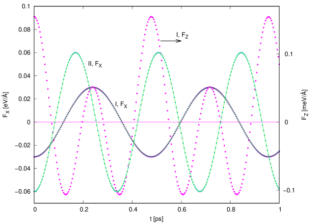
Figure 10: Comparison of forces $F_{X}(t)$ and $F_{Z}(t)$ in two simulations, I and II, as described in the text. The amplitude of X displacement is 0.03 Å.

When an external pressure is applied in the X-direction, forces acting on layers in the Z-direction must have a contribution from two mechanisms: one is obviously due to a harmonic motion in the Z-direction. That part ought to be given by $-k\cdot\Delta Z$, where k is the same spring constant as the one describing the motion in the X-direction under force in the same direction. The second part, as already argued, is caused by a nonlinear contribution that is in the direction perpendicular to X axis, and it is defined as $\kappa\cdot\Delta X^{2}$. Therefore, the entire force $F_{Z}$ must be given as

$$F_{Z}(t)=-k\cdot\Delta Z(t)+\kappa\cdot\Delta X^{2}(t).$$ (18)

That relation is checked in figure 11. There we compare the value determined from simulations, with a value computed by using 18 and the data on $\Delta X(t)$ and $\Delta Z(t)$ taken also from simulations. Hence, this is an illustration of how a mixing of X- and Z-components of the movement must be taken into account for a proper description of dynamics, which is in agreement with the Newtonian mechanics.

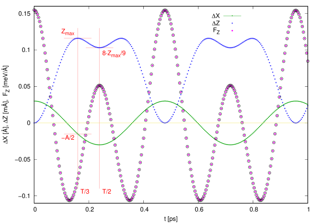
Figure 11: Testing the relation $F_{Z}(t)=-k\cdot\Delta Z(t)+\kappa\cdot\Delta X^{2}(t)$. Notice different vertical scales and units for each quantity. The green line shows $\Delta X(t)$, the blue dots are $\Delta Z(t)$, magenta dots is the $F_{Z}(t)$ dependence. All these are determined from MD simulations. All the data are from the same simulation run as these used in figure 10. Large empty black circles are computed by using the above formula, with the value of $\kappa$ determined as described in Fig. 6.

Let us now discuss another type of phase-space diagram, for the case when the upper layer is moved, by using the same or similar simulations data as these were used to draw figures 10 and 11. In figure 12 a) dependencies of $\Delta Z$ on $\Delta X$ are shown at short times $t\lessapprox T$ (where T is the oscillation period) for 3 values of the initial amplitude A, when $\alpha=0^{\circ}$. For all 3 curves, the X-axis scales up linearly with A, and the Z-axis scales up as A².

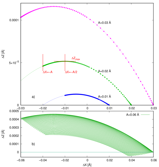
Figure 12: X-Z phase-space portraits when $\alpha=0^{\circ}$, for 3 values of the amplitude A of initial displacement $\Delta X$, 0.01, 0.02 and 0.03 Å. Time is the hidden parameter there. The simulation data are shown as points. The maximum of $\Delta Z$ is observed when $\Delta X=-A/2$ and it has a value of $Z_{max}$. The curves are well described by parabolic functions (shown by continuous lines). The data are shown for short times, covering around one full period of oscillations. After the particle arrives from the right direction to the most left point located at $\Delta X=-A$, the motion is continued back in the right direction on the same curve. In b) we show similar curves for a larger amplitude A=0.06 Å and for a much longer time range, as an illustration of the hysteretic nature of oscillations.

Since forces in the Z-direction are several orders lower in magnitude than in the X-direction, we may assume as an approximation that the movement in the X-direction is not influenced by $F_{Z}$. Hence, $\Delta X(t)$ must be given by a simple harmonic function fulfilling the initial boundary condition $\Delta X(t=0)=A$, that is: $\Delta X(t)=A\cdot\cos(\Omega t)$. Hence, while X(t=0)=A, the minimum value of X is at t=T/2, i.e., $X(\Omega T/2)=-A$. The initial value of Z is $Z(t=0)=0$. The time $t=T/2$ is the return point. It follows from the data analysis that the maximum value of $\Delta Z(t)$, which is $Z_{max}$, is observed when $\Delta X(t)=-A/2$ (compare red horizontal and vertical bars in figures 11 and 12 a). Hence, it occurs at $t=T/3$. At this moment we do not have a derivation of equations of motion allowing us to find an analytical expression on $\Delta Z(\Delta X)$. It is evident, however, that with a large confidence and accuracy we can approximate that dependence as a parabolic one, and it must be given by the following formula fulfilling all the required boundary conditions and the observed properties:

$$\Delta Z=Z_{max}[1-(4/9)(\Delta X/A+1/2)^{2}],$$ (19)

We find from 19 the value of $\Delta Z$ at $\Delta X=-A$ as $8Z_{max}/9$.

Actually, there is a hysteresis there (hardly observable at these low amplitudes and short times). It is seen better in 12 b) drawn for a larger amplitude of oscillation, A=0.06 Å, and for a much longer time range.

3.4 Equations of motion in X-Z plane.

Since $\Delta X(t)=A\cdot\cos(\Omega t)$, and $F_{Z}(t)=\kappa(\Delta X(t))^{2}-k\Delta Z(t)$, and $\rm{m}\cdot d^{2}\Delta Z(t)/dt^{2}=F_{Z}$, $k/\rm{m}=\Omega^{2}$, we are able to write the following differential relation:

$$d^{2}\Delta Z(t)/dt^{2}=\kappa/\rm{m}\cdot A^{2}\cdot\cos^{2}(\Omega t)-\Omega^{2}\cdot\Delta Z(t),\penalty 10000\ \penalty 10000\ \penalty 10000\ \Delta Z(0)=0,V_{Z}(0)=0.$$ (20)

In order to simplify notation, let us replace $\Delta Z(t)$ by $z(t)$. Let us also use the relation $\cos^{2}(x)=(1+\cos(2x))/2$. Now, 20 can be written as

$$\ddot{z}=\frac{\kappa A^{2}}{2\rm{m}}\cdot\left(1+\cos(2\Omega t)\right)-\Omega^{2}\cdot z.$$ (21)

We recognize that 21 is an equation of a driven harmonic oscillator (see, e.g., [10]), with a driving force of angular frequency $2\Omega$. One can simply check that 19 is a solution of 21 when we use

$$Z_{max}=3\kappa A^{2}/(4\rm{m}\Omega^{2}).$$ (22)

Equation 21 and its solution 19 may be treated as approximations only, valid at short times $t\lessapprox T$. In particular, these equations do not provide a description of the mechanism and dynamics of hysteretic phenomena, as shown in figure 12 b). In 21 it is taken into account only that any displacement in the X-direction causes a movement of the particle in the Z-direction. It does not account for anharmonicity of potential caused by movement of particles in the Z-direction.

The description used in this section can be extended to analysis of oscillations in arbitrary direction, for showing another, alternate method of finding the angular dependence $\kappa(\alpha)$. Let us restrict ourselves this time to providing the algorithm only of the data analysis, without giving its detailed explanations.

1) For any data obtained from simulations performed at an angle $\alpha$ with respect to the X-axis, we draw the difference between $\Delta Z$ and $\tan(\alpha)\cdot\Delta X$ as a function of $\Delta X$, as shown in figure 13.

2) By using the method of least-squares fitting, we determine the parameters of the parabolic dependencies shown there.

3) The true parameter $Z_{max}$ for any given $\alpha$ is obtained by multiplying the one from step 2) by $\cos(\alpha)$.

Using 22, $\kappa$ can be found from $\kappa=4\rm{m}\Omega^{2}/(3A^{2})\cdot Z_{max}$. We do not show the results on $\kappa(\alpha)$ this time because they are practically identical to these shown in figure 9. With the mass of 1 atom of Fe, $\rm{m}=9.273\cdot 10^{-26}kg$, $\Omega=13.144/ps$, the initial amplitude of oscillations A=0.02 Å, we found out that the best-fitting gives us the angular dependence: $\kappa(\alpha)=\kappa_{0}\cdot\cos(3\alpha)$, with $\kappa_{0}$=0.17197 eV/ų, while in figure 9 $\kappa_{0}$=0.1717 eV/ų was obtained, and the value computed from first principles in subsection 3.1 is 0.1720 eV/ų.

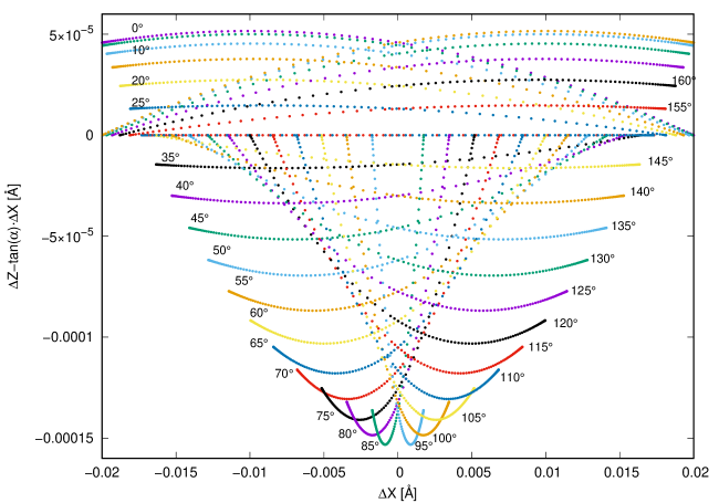
Figure 13: Dependence of $\Delta Z-\tan(\alpha)\cdot\Delta X$ on $(\Delta X)$, determined from initial oscillations, when the layer is displaced for 0.02 Å in a direction $\alpha$ with respect to the X-axis. The labels indicate the angle $\alpha$.

4 Discussion.

4.1 A connection with Christoffel equations.

In the theory of elastic waves in crystals, Christoffel equations[11, 12, 13, 14, 15] relate the static elastic constants with possible directions of plane waves propagation and their polarization (velocity vectors of the displacement of atoms) [16]. For an FCC crystal, there are only three independent elastic constants[12]. We determined values of stiffness parameters by using the method of Sprik et al [17] available in the source code distribution of lammps [6] through a package written by Aidan Thompson. The values are: $C_{11}$=180 GPa, $C_{12}$=90 GPa, and $C_{44}$=90 GPa.

In the case of waves traveling in the [1,1,1] direction, values of corresponding sound velocities are ($\rho$ is density): $c_{L}=\left((C_{11}+2C_{12})+4C_{44})/3\rho\right)^{1/2}$ (the longitudinal one) and $c_{T}=\left((C_{11}-C_{12}+C_{44})/3\rho\right)^{1/2}$ (two degenerate transverse components; compare this with Levy [12]). Hence, we compute: $c_{L}$=54.031Å/ps and $c_{T}$=27.016 Å/ps. $c_{T}$ can be found easily from data like these in figures 1-3, while $c_{L}$ from similar simulations, when a Heaviside pressure is applied along the Y-direction. Values of the sound speed components found from MD simulations are in very good agreement with these computed above, when simulations are performed in the limit of very small applied pressure (let say below 10 MPa).

Eigenvectors of Christoffel equations determine polarization of velocities. The longitudinal velocity is in the [1,1,1] direction. The other two, degenerate transversal velocities, are in directions [1, 0, $\bar{1}$] and [0, 1, $\bar{1}$] (figure 14). Some authors suggest (e.g., Levy [12], p. 18.) that it does not matter what is the direction of oscillations of the transverse wave, as long as its displacement component lies within the (1,1,1) plane. That seems a natural assumption since Christoffel equations are linear ones and therefore solutions in any direction within that plane can be constructed as a linear combination of two transverse components in directions [1, 0, $\bar{1}$] and [0, 1, $\bar{1}$]. In our case, as it follows from the angular dependence of equipotential diagrams (7 and 8) as well as from figure 9, angles of $30\mathrm{°}$ ($\pm$ integer multiplicities of $60\mathrm{°}$), have a special meaning: the contribution to the particle motion that is perpendicular to the applied force disappears. These are directions that are perpendicular to one of the eigenvectors that are solutions to Christoffel equations (figure 14). At first sight one might think that at these special angles we are in the limit of a linear problem, since coupling between the movement in the $\hat{r}$ and $\hat{\alpha}$ directions disappears. However, this is a wrong assumption: we do observe at these angles (not shown) a strong dependence of MD simulation results on the amplitude of the applied force. It must be due to a non-harmonicity of the potential as a function of distance from x=z=0. In fact, the nonlinear contribution to the potential has a different sign for angles, for instance, $+30\mathrm{°}$ and $-30\mathrm{°}$, as can be seen in figure 8. Therefore, Christoffel equations may be treated as an approximation only and could be considered valid in the limit of very small pressure applied only.

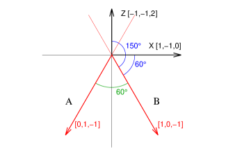
Figure 14: Eigenvectors of solutions to Christoffel equations for transverse waves traveling in the [1,1,1] direction.

4.2 Analytical solutions of equations of motion in a CSM model.

Exact analytical solutions of equations of motion in a CSM model [4] are derived from a set of linear difference equations:

$${\ddot{x}}_{n}+2{{\rm{\Omega}}}^{2}{x}_{n}-{{\rm{\Omega}}}^{2}{x}_{n+1}-{{\rm{\Omega}}}^{2}{x}_{n-1}=0,$$ (23)

with the boundary condition:

$${\ddot{x}}_{1}+{{\rm{\Omega}}}^{2}({x}_{1}-{x}_{2})={F}_{1}(t)/\rm{m},$$ (24)

where $x_{n}$ is the displacement of the n-th layer, $F_{1}(t)$ is the time-dependent force acting on the layer 1, and $\Omega$ is the angular frequency of a single mass $\rm{m}$ with spring constant $k$ of harmonic interaction between two masses, $\Omega=\sqrt{k/\rm{m}}$.

In our case the situation requires an additional set of equations like these for the z-component of displacement, with proper boundary conditions on forces acting in the z-direction at the surface (layer 1). New equations must contain an additional term that is responsible for forces acting in z-direction when the particle/layer moves in the x-direction.

The additional term acting on the n-th particle in the x-direction will depend on the second power of the difference of z-positions between particles n-1 and n+1. Hence, if an extra force in the x-direction is defined as $\kappa\cdot(z_{n+1}-z_{n-1})^{2}$ than, instead of equation 23, we ought to have:

$${\ddot{x}}_{n}+2{{\rm{\Omega}}}^{2}{x}_{n}-{{\rm{\Omega}}}^{2}{x}_{n+1}-{{\rm{\Omega}}}^{2}{x}_{n-1}-(\kappa/m)\cdot(z_{n+1}-z_{n-1})^{2}=0.$$ (25)

One might think that in a similar way equations for displacements in the Z-direction ought to be written:

$${\ddot{z}}_{n}+2{{\rm{\Omega}}}^{2}{z}_{n}-{{\rm{\Omega}}}^{2}{z}_{n+1}-{{\rm{\Omega}}}^{2}{z}_{n-1}-(\kappa/m)\cdot(x_{n+1}-x_{n-1})^{2}=0.$$ (26)

However, if to consider a movement in the Z-direction (equation 26), we would need to use there $\kappa=\kappa_{0}$, while for Z-direction (equation 25), $\kappa=0$, as it follows from 17. Moreover, as mentioned in the previous subsection, an anharmonic contribution to forces, due to the dependence of potential on r, must be taken into account as well.

Coupled equations 25 and 26 may not have a closed-form exact analytical solution. One could possibly find its approximate numerical solutions by using an iterative method. We know already that in the limit of very small forces, solutions tend to these in the linear case, when the precession of the movement may be ignored. At large forces, MD simulations offer an excellent alternate way of studying properties of its solutions.

4.3 Other comments.

The resulting dynamics is a complex one, as illustrated in figure 12 b). The relaxation of the amplitude of oscillations there is not a simple exponential function of time: it combines nonlinearity and chaos. This is a field requiring an additional systematic exploration.

The presented model implies the existence of a displacement of layers in the Z-direction when a force is applied in the X-direction. This effect is a dynamic one, and it is inconsistent with the static theory. However, it becomes significant only at large applied forces, since it is proportional to the square of pressure, it may have been overlooked in experiments. Additionally, until systematic investigation of the role of chaos is learned, we can not be sure how large it could be in real materials of macroscopic size. It might be worth considering an experimental verification of this phenomenon (and a few other related ones, not mentioned here) on crystals, and also on artificial acoustic metamaterials.

5 Conclussions.

A dynamical effect has been observed in MD simulations and explained by a simple mechanism, supported by an analytical model. It is caused by broken symmetry of interaction between neighboring crystallographic layers, caused by propagating stress waves. The effect is not due to the displacement between the nearest layers alone, but due to the difference between displacements of layers on both sides of any given layer. A traveling stress wave causes that difference. Hence, this is not a surface effect but a bulk one. We describe it with an example of a particular crystallographic orientation of an FCC crystal. However, it ought to be present also in some other simulation setups, when there is a difference between atomic configurations on two sides of a layer, when stress waves travel in a perpendicular direction to layers.

One of the consequences is, in our case, a broken axial symmetry in the (111) plane, leading to a threefold symmetry instead, as demonstrated by simulations of angular dependence of forces, as well as a nonzero shear displacement in Z-direction when force is applied in the X-direction. We expect that such a displacement ought to be observable in experiments, performed at appropriate conditions. These effects are proportional to the square of applied forces and therefore their amplitude tends to zero when forces are small.

While the simulation setup used in the experiments described here has been simplified as much as possible (harmonic interlayer potential is used with an ideal mono-atomic crystal structure) the results of simulations performed by us on more realistic structures (several kinds of FCC compounds, with various types of atoms and atomistic potentials) are qualitatively the same. In particular, we observe lattice displacements and large forces in the Z-direction, of a similar, oscillating in time/position nature when the front of a stress wave propagating in the Y-direction hits a layer. The effect raises a question, in particular, about its role in the dynamics of the movement of dislocations.

6 References

References

- [1] Schrödinger E 1914 Ann. Phys. 349(14) 916–934
- [2] Mühlich U, Abali B E and dell’Isola F 2021 Mathematics and Mechanics of Solids 26(1) 133–147
- [3] de Pater A D 1974 Vehicle System Dynamics: International Journal of Vehicle Mechanics and Mobility 3:3 123–140
- [4] Kozioł Z 2025 J. Phys. Commun. 9 045005 URL https://doi.org/10.1088/2399-6528/adcdbf
- [5] Zhao S, Osetsky Y N and Zhang Y 2017 J. Alloy Comp. 701 1003–1008
- [6] Plimpton S 1995 J. Comp. Phys. 117 1
- [7] Kozioł Z 2024 Modelling Simul. Mater. Sci. Eng. 32 055010 URL https://doi.org/10.1088/1361-651X/ad4575
- [8] Kozioł Z 2024 Harmonic interlayer potential with no higher-order contributions. V2 Mendeley Data URL https://data.mendeley.com/datasets/4s6sy4b4nf/2
- [9] Kozioł Z 2024 Averaging positions, velocities, forces, etc., for atoms in crystallographic layers. V1 Mendeley Data URL https://data.mendeley.com/datasets/tnf7fg3m4g/1
- [10] Thornton S and Marion J 2003 Classical Dynamics of Particles and Systems 5th ed (Pacific Grove, CA: Brooks Cole)
- [11] Fedorov F I 1968 Theory of Elastic Waves in Crystals (Springer)
- [12] Levy M 2001 Experimental Methods in the Physical Sciences 39 1–35
- [13] Ting T 2006 Acta Mechanica 185 147–164
- [14] Ting T 2006 Wave Motion 44 107–119
- [15] Jan W Jaeken S C 2016 Computer Physics Communications 207 445–451
- [16] Lynch S 2018 Dynamical Systems with Applications using Python. (Birkhäuser) ISBN 9783319781457
- [17] Sprik M, Impey R W and Klein M L 1984 Phys. Rev. B 29 4368