Decision Potential Surface: A Theoretical and Practical Approximation of LLM’s Decision Boundary

Abstract

Decision boundary, the subspace of inputs where a machine learning model assigns equal classification probabilities to two classes, is pivotal in revealing core model properties and interpreting behaviors. While analyzing the decision boundary of large language models (LLMs) has raised increasing attention recently, constructing it for mainstream LLMs remains computationally infeasible due to the enormous vocabulary-sequence sizes and the auto-regressive nature of LLMs. To address this issue, in this paper we propose Decision Potential Surface (DPS), a new notion for analyzing LLM decision boundary. DPS is defined on the confidences in distinguishing different sampling sequences for each input, which naturally captures the potential of decision boundary. We prove that the zero-height isohypse in DPS is equivalent to the decision boundary of an LLM, with enclosed regions representing decision regions. By leveraging DPS, for the first time in the literature, we propose an approximate decision boundary construction algorithm, namely $K$-DPS, which only requires $K$-finite times of sequence sampling to approximate an LLM’s decision boundary with negligible error. We theoretically derive the upper bounds for the absolute error, expected error, and the error concentration between $K$-DPS and the ideal DPS, demonstrating that such errors can be trade-off with sampling times. Our results are empirically validated by extensive experiments across various LLMs and corpora.

1 Introduction

With the rapid advancement and remarkable success of large language models (LLMs), understanding their underlying mechanisms and behaviors has become increasingly critical (Wang et al., 2023; Conmy et al., 2023; Elhage et al., 2021; Ameisen et al., 2025; Sharkey et al., 2025; Allen-Zhu & Li, 2023; Liang et al., 2025; 2024). A key approach to demystifying the “black box” of state-of-the-art AI models involves analyzing the decision boundary (Rosenblatt, 1958), a fundamental concept for elucidating the characteristics of machine learning (ML) models. For LLMs, decision boundaries provide valuable insights into critical phenomena, including reasoning (Yang et al., 2025b), in-context learning (Zhao et al., 2024), hallucination (Mayne et al., 2025), memorization (Li et al., 2025), and so on.

As a foundational concept in machine learning, the decision boundary represents a subspace of inputs where a model assigns equal probability to two distinct classification outcomes (Rosenblatt, 1958). Extensive theoretical and empirical studies (Lee & Oommen, 1997; Turner & Ghosh, 1996; Goodfellow et al., 2015; Madry et al., 2018; Gu et al., 2017) have demonstrated that the properties of decision boundaries reveal critical attributes of machine learning models, including performance, robustness, and generalization. Consequently, constructing and leveraging decision boundaries for LLMs become a powerful and promising approach to enhance almost all downstream analyses of their behavior and capabilities.

Unfortunately, analyzing decision boundaries of LLMs incurs significantly greater complexity than on deep neural networks (DNNs) (Karimi et al., 2020; Karimi & Tang, 2020; Li et al., 2019; Lee & Landgrebe, 1997; Mickisch et al., 2020; Yousefzadeh & O’Leary, 2019). Unlike classification tasks with a limited number of classes (Lee & Oommen, 1997; Turner & Ghosh, 1996; Goodfellow et al., 2015; Madry et al., 2018; Gu et al., 2017), LLMs predict a single token from an expansive vocabulary, often exceeding 100,000 tokens. Moreover, their autoregressive nature (Bengio et al., 2003; Radford et al., 2018) requires iterative token predictions to generate complete sequences, which further compounds the complexity of modeling decision boundaries. For instance, a Qwen-3 model (with 8 billion parameters) (Yang et al., 2025a) supports sequences up to 32,768 tokens with a vocabulary of 151,936, resulting in approximately $10^{169,790}$ decision regions! Such an enormous scale renders trivial attempts on decision-boundary-based analysis or visualization computationally infeasible. Prior studies (Zhao et al., 2024; Yang et al., 2025b; Mayne et al., 2025; Li et al., 2025), despite their valuable contributions to their specific motivating tasks, unfortunately sidestep this critical challenge. They either simplify the problem to toy scenarios, such as binary classification (Zhao et al., 2024; Mayne et al., 2025), or use the decision boundary concept metaphorically without constructing it (Yang et al., 2025b; Li et al., 2025). Consequently, the haunting questions remain unanswered — What constitutes an LLM’s decision boundary, and is there a universal and yet efficient algorithm to construct it?

To address these questions, we propose a principled strategy for modeling the decision boundaries of LLMs, which yields theoretical guarantees, computational tractability, and interpretability simultaneously. Inspired by the existing decision boundaries for multi-class classification, we treat generative language models as a composite multi-class classification task. As trivial solutions cannot model the complex decision boundaries for such tasks, we introduce a novel concept, namely Decision Potential Surface (DPS), to facilitate decision boundary analysis. It is a landscape in which every point encodes the competition potential among candidate outputs, quantified by a decision potential function (DPF). We theoretically demonstrate that the zero-height isohypse of the DPS corresponds to the decision boundary, with the enclosed regions representing decision regions.

By examining the definition of DPS, we surprisingly discover that enumerating the entire output space is unnecessary for computing the DPF. Instead, a sufficient sampling already captures the “competition potential”. We therefore approximate the LLM’s decision boundary with only $K$-finite ($K\ll$ realistic classification count) sequence sampling, yielding $K$-DPS and keeping the theoretical error within a provably small bound. We establish the error bound, expected error bound, and error concentration between the ideal DPS and $K$-DPS, demonstrating that $K$-DPS offers a favorable trade-off between approximation accuracy and computational cost. Finally, we conduct extensive experiments on open-source LLMs to evaluate the empirical performance of our method.

To the best of our knowledge, this is the first study on constructing decision boundaries for LLMs. Moreover, our proposed decision potential surface (DPS) framework is the first to provide a practical approximation of decision boundaries with theoretical guarantees. Our contributions are as follows:

• We formalize the definition of an LLM’s decision boundary as a composite multi-class classification task and analyze its fundamental properties.

• We introduce the concepts of the Decision Potential Function (DPF) and Decision Potential Surface (DPS). We prove that the isohypses of the decision potential surface represent the marginal decision boundaries of LLMs, with the zero-height isohypse equivalent to the decision boundary.

• We propose $K$-DPS, an efficient and bounded approximation of the ideal DPS that requires only finite sampling for each input. We theoretically and empirically establish the error bounds of this approximation relative to the ideal DPS and quantify the trade-off between approximation error and sampling size.

2 Related Works

Decision Boundary Analysis on Machine Learning Models. The earliest exploration of decision boundaries in neural networks dates back to the era of linear classifiers and shallow architectures. Rosenblatt (1958) introduced the first linear decision boundary for binary classification, where a hyperplane separates input samples into two classes. For shallow feedforward neural networks (FFNNs) with non-linear activations (e.g., sigmoid, ReLU), subsequent work quantified how hidden layers enable non-linear decision boundaries: Lee & Oommen (1997) proposed a feature extraction method that maps input data to a space aligned with FFNN decision boundaries, showing that boundary curvature correlates with model capacity and classification accuracy. For ensemble neural networks, Turner & Ghosh (1996) made a pivotal contribution: they developed a theoretical framework that connects the stability of decision boundaries (relative to the optimal boundary defined by Bayes theory) to the overall error performance of the ensemble. Their work showed that linearly combining multiple well-designed, unbiased neural classifiers can reduce fluctuations in decision boundaries, which in turn lowers the extra error that goes beyond the theoretical minimum (i.e., Bayes error). A critical insight established by this finding is that the geometric characteristics of decision boundaries are closely tied to how well a model performs, which sheds light on employing decision boundary to explain the properties of neural networks.

Decision Boundary Analysis on Neural Networks. In recent years, researchers extended boundary analysis to convolutional neural networks (CNNs) and transformers for computer vision (CV) tasks. Goodfellow et al. (2015) revealed a key vulnerability of deep CNNs: their decision boundaries are locally linear in high-dimensional input spaces, making them susceptible to adversarial examples. Madry et al. (2018) further formalized this by proving that robust training (e.g., adversarial training) “smooths” decision boundaries, reducing local linearity and adversarial susceptibility. Similarly, Gu et al. (2017) focused on backdoor attacks in CNNs, linking them to hidden ”trapdoors” in decision boundaries. Such attacks involve planting a small, specific pattern that shifts the boundary and forces misclassification for triggered inputs. Lee & Landgrebe (1997) laid the groundwork by introducing decision boundary feature extraction, highlighting the boundary’s role in characterizing network behavior before deep learning. Later, Yousefzadeh & O’Leary (2019) examined trained networks’ decision boundaries, analyzing how architectural elements (e.g., depth and activation functions) and training data influence boundary shape, complexity, and stability, providing insights into network task performance. Mickisch et al. (2020) conducted an empirical study on deep network boundaries across CV tasks, including image classification and object detection. Via quantitative and qualitative analysis, they explored boundary behavior near correct and misclassified samples and adversarial examples, bridging theory-practice gaps. In the same year, Karimi & Tang (2020) reviewed boundary research challenges such as high input dimensionality, complex architectures, and limited visualization tools, and opportunities, including advanced math, innovative visualization, and robustness enhancements. Karimi et al. (2020) complementarily proposed metrics like smoothness, curvature, and class separation to quantify boundaries, enabling cross-model comparisons and standardized analysis for deep learning interpretability.

Decision Boundary Analysis on Large Language Models. Extending decision boundary analysis from traditional neural networks (e.g., CNNs) to LLMs, researchers have begun exploring how this concept illuminates LLMs’ decision-making mechanisms and limitations. Zhao et al. (2024) probed the decision boundaries of in-context learning in LLMs, shedding light on how contextual information shapes boundary formation and decision outputs. Li et al. (2025) surveyed LLMs’ knowledge boundaries, laying a foundation for linking knowledge scope to decision boundaries. Mayne et al. (2025) revealed LLMs’ ignorance of their own decision boundaries and the unreliability of self-generated counterfactual explanations. Yang et al. (2025b) proposed BARREL, a boundary-aware reasoning framework to enhance LLM factuality via boundary awareness.

However, existing work fails to address LLM decision boundary analysis core challenges: Zhao et al. (2024) and Mayne et al. (2025) simplify to binary classification toy scenarios, deviating from LLMs’ real multi-token autoregressive prediction; Yang et al. (2025b) and Li et al. (2025) use the decision boundary concept metaphorically without concrete construction methods, unable to tackle exponential decision region complexity. This leaves a lack of universal, computationally feasible, and theoretically grounded boundary-capturing approaches, hindering LLM interpretation and optimization. Therefore, this paper aims to propose new decision boundary theory for addressing high-dimensional complexity and construction barriers, enabling accurate, efficient, and interpretable boundary modeling aligned with LLMs’ characteristics.

3 Preliminaries: Decision Boundary of Language Models

3.1 Decision Boundary and Its Geometry on Classification Models

We begin our theoretical analysis with traditional classification models and aim to extend the insights to generative language models.

Consider a neural network $f:\mathbb{R}^{d}\to\mathbb{R}^{M}$ that maps an input sample $\mathbf{x}\in\mathbb{R}^{d}$ to a predicted probability distribution over $M$ classes, $\mathcal{M}=\{1,2,\dots,M\}$. $M>2$. Our goal is to characterize the properties of $f$ under a specific input data distribution $\mathcal{D}\subseteq\mathbb{R}^{d}$. Without loss of generality, we decompose $f$ into three components: (i) A representation module $h=f_{r}(\mathbf{x}):\mathbb{R}^{d}\to\mathbb{R}^{d^{\prime}}$ that maps the input $\mathbf{x}$ to a latent representation $h$. (ii) A linear classification head $z=f_{\text{cls}}(h)=W_{\text{cls}}h+b_{\text{cls}}:\mathbb{R}^{d^{\prime}}\to\mathbb{R}^{M}$, where $W_{\text{cls}}\in\mathbb{R}^{M\times d^{\prime}}$ and $b_{\text{cls}}\in\mathbb{R}^{M}$ are learnable parameters, projecting the representation $h$ into classification logits $z$. (iii) A nonlinear normalization function $P=\sigma(z):\mathbb{R}^{M}\to\mathbb{R}^{M}$, which transforms the logits into a probability distribution $P=[p_{1},p_{2},\dots,p_{M}]$, where $0\leq p_{i}\leq 1$ for $i=1,\dots,M$ and $\sum_{i=1}^{M}p_{i}=1$. The final predicted class for $\mathbf{x}$ is determined by $\arg\max_{i}p_{i}$. Then, the decision boundary of the neural network is defined as follows.

Definition 3.1 (Decision Boundary of $f$).

The decision boundary of a neural network $f$ under an input distribution $\mathcal{D}$ is the set of inputs $\mathbf{x}\in\mathcal{D}$ for which at least two classes in $\mathcal{M}=\{1,2,\dots,M\}$ have equal and maximal prediction probabilities. Formally, we denote this set as $\mathcal{B}_{M}^{(f,\mathcal{D})}$, defined by:

$$\mathcal{B}_{M}^{(f,\mathcal{D})}=\left\{\mathbf{x}\in\mathcal{D}\mid\exists~m,n\in\mathcal{M},m\neq n,\text{ such that }p_{m}=p_{n}\text{ and }p_{m}\geq\max_{o\in\mathcal{M}\setminus\{m,n\}}p_{o}\right\},$$ (1)

where $p_{i}=P[i]=\sigma(f_{\text{cls}}(f_{r}(\mathbf{x})))[i]$ is the predicted probability for class $i$.

Based on Definition 3.1, we characterize the decision boundary for multi-class classification scenarios as follows.

Theorem 3.2 (Properties of Multi-Class Classification Boundary).

For multi-class classification ($M>2$), the decision boundary of $f$ can be expressed as:

$$\quad\quad\quad\quad\quad\quad\quad\quad\quad\quad\quad\quad\mathcal{B}_{M}^{(f,\mathcal{D})}=\bigcup_{1\leq m<n\leq M}\mathcal{B}_{mn},$$ (2)

$$\mathcal{B}_{mn} =\left\{\mathbf{x}\mid(w_{m}-w_{n})h+(b_{m}-b_{n})=0,\,z_{m}=z_{n}\geq z_{o}\,\forall o\neq m,n,\,h=f_{r}(\mathbf{x}),\,\mathbf{x}\in\mathcal{D}\right\}.$$

where $z=W_{cls}h+b_{cls}$ is the logits, $w_{m}$ and $w_{n}$ are the $m$-th and $n$-th rows of $W_{\text{cls}}$, and $b_{m},b_{n}$ are the corresponding entries of $b_{\text{cls}}$.

Geometrically, $\mathcal{B}_{M}$ induces a Voronoi partition of the representation space, where each class corresponds to a Voronoi cell.

The proof of Theorem 3.2 is provided in Appendix B.1.

3.2 Decision Boundary for Large Language Models

An LLM $f:\mathcal{V}^{N_{q}}\to\mathcal{V}^{N_{r}}$ generates a sequence of tokens $\mathbf{y}=[y_{1},\dots,y_{N_{r}}]$, where each token $y_{t}\in\mathcal{V}=\{1,2,\dots,V\}$ is drawn from a vocabulary of size $V$, conditioned on an input prompt $\mathbf{x}=[x_{1},\dots,x_{N_{q}}]\in\mathcal{V}^{N_{q}}$. $N_{q}$ and $N_{r}$ are sequence length of the input and the generated texts. At each generation step $t$, the LLM predicts the next token $y_{t}$ based on the prompt and previously generated tokens, i.e., $y_{t}\sim P_{f}(y_{t}|\mathbf{x},y_{1},\dots,y_{t-1})$. This single step generation can be viewed as a multi-class classification over $\mathcal{V}$, and thus, the single-token decision boundary follows Theorem 3.2. When defining the decision boundary for the entire sequence $\mathbf{y}\in\mathcal{V}^{N_{r}}$, we need to firstly model the joint probability of the sequence under the autoregressive process.

Theorem 3.3 (Decision Boundary of Language Models).

The decision boundary of an LLM $f$ under an input text distribution $\mathcal{D}^{\prime}\subseteq\bigcup_{n_{q}=1}^{N_{q}}\mathcal{V}^{n_{q}}$ is the set of prompts $\mathbf{x}\in\mathcal{D}^{\prime}$ that lead to equal generation probabilities for at least two distinct sequences $\mathbf{y}_{v},\mathbf{y}_{w}\in\mathcal{V}^{N_{r}}$, with their probabilities being maximal. Formally, the decision boundary $\mathcal{B}_{llm}^{(f,\mathcal{D}^{\prime})}$ is defined as:

$$\mathcal{B}_{llm}^{(f,\mathcal{D}^{\prime})} =\bigcup_{\mathbf{y}_{v}\neq\mathbf{y}_{w}\in\mathcal{V}^{N_{r}}}\mathcal{B}_{llm,vw},$$ (3)

$$\mathcal{B}_{llm,vw} =\left\{\mathbf{x}\in\mathcal{D}^{\prime}\mid P_{f}(\mathbf{y}_{v}|\mathbf{x})=P_{f}(\mathbf{y}_{w}|\mathbf{x})\geq\max_{\mathbf{y}_{u}\in\mathcal{V}^{N_{r}}\setminus\{\mathbf{y}_{v},\mathbf{y}_{w}\}}P_{f}(\mathbf{y}_{u}|\mathbf{x})\right\},$$

where $P_{f}(\mathbf{y}|\mathbf{x})=\prod_{t=1}^{N_{r}}P_{f}(y_{t}|\mathbf{x},y_{1},\dots,y_{t-1})$ is the joint probability of generating sequence $\mathbf{y}$ given prompt $\mathbf{x}$.

The proof of Theorem 3.3 is provided in Appendix B.2.

While Theorem 3.3 provides a concise and intuitive definition of the decision boundary for LLMs, analyzing or computing this boundary could be computationally impossible in practice. As analyzed in Section 1, the primary challenge stems from the large vocabulary size and the autoregressive nature of sequence generation, i.e., for a generation of length $N_{r}$, the total number of possible sequences is $V^{N_{r}}$, leading to an exponential growth in the classification space. Specifically, the decision boundary defined in Equation equation 3 involves comparing pairs of sequences $\mathbf{y}_{v},\mathbf{y}_{w}\in\mathcal{V}^{N_{r}}$, resulting in up to $\binom{V^{N_{r}}}{2}\approx\frac{(V^{N_{r}})^{2}}{2}$ pairwise comparisons. This is neither computationally feasible nor interpretable on subsequent visualization.

Given such intractability of directly analyzing the decision boundary defined in Theorem 3.3, a new strategy for constructing the decision boundary of large language models is essential. Specifically, we hope that this new construction satisfies the following criteria: First, it must be theoretically rigorous, meaning the construction should be equivalent to or provide a bounded approximation of the decision boundary defined in Theorem 3.3, ensuring consistency with the formal definition of the boundary separating prompts that yield different output sequences. Second, the method should be practical, meaning it must be computationally efficient and feasible for implementation, enabling the modeling of decision boundaries for industrial-scale LLMs with large vocabularies and long generation lengths. Third, the method should be interpretable, meaning the constructed decision boundary should explicitly capture key properties of LLMs (e.g., curvature), and provide interpretable insights into phenomena observed in LLM behavior, such as output variability or robustness.

In the next section, we will introduce an approximation procedure for the decision boundary defined in Theorem 3.3, addressing these criteria to enable practical and meaningful analysis of LLMs.

4 Decision Potential Surface: Simplifying Decision Boundary Analysis on Large Language Models

In this section, we introduce the Decision Potential Surface (DPS), a novel concept for analyzing the decision boundaries of LLMs by representing the decision potential of generated sequences as a surface over the input manifold. In Section 4.1, we formally define DPS and establish its relationship with the standard decision boundary formulation in LLMs. In Section 4.2, we propose $K$-grained DPS ($K$-DPS), a practical approximation of DPS, and theoretically derive its error bounds with respect to the ideal DPS.

4.1 Decision Potential Surface of Language Models

Definition 4.1 (Decision Potential Surface of Language Models).

Given an input text distribution $\mathbf{x}\in\mathcal{D}^{\prime}$ with $\mathcal{D}^{\prime}\subseteq\bigcup_{n_{q}=1}^{N_{q}}\mathcal{V}^{n_{q}}$ and a language model $f:\mathcal{V}^{N_{q}}\to\mathcal{V}^{N_{r}}$ that generates an output sequence $\mathbf{y}=f(\mathbf{x})=\arg\max_{\mathbf{y}_{s}\in\mathcal{V}^{N_{r}}}P_{f}(\mathbf{y}_{s}|\mathbf{x})$, we define the decision potential function (DPF) $\Phi_{f}^{\infty}(\mathbf{x}):\mathcal{D}^{\prime}\to\mathbb{R}_{+}$ as the squared difference in log-likelihoods between the top two generated sequences under the input prompt $\mathbf{x}$, i.e.,

$$\Phi_{f}^{\infty}(\mathbf{x}) =\left(\min_{\mathbf{y}_{w}\in\mathcal{V}^{N_{r}},\mathbf{y}_{w}\neq\mathbf{y}_{v}}\left[\max_{\mathbf{y}_{v}\in\mathcal{V}^{N_{r}}}\log P_{f}(\mathbf{y}_{v}|\mathbf{x})-\log P_{f}(\mathbf{y}_{w}|\mathbf{x})\right]\right)^{2}$$ (4)

$$=\big(\log P_{f}(\mathbf{y}_{1*}|\mathbf{x})-\log P_{f}(\mathbf{y}_{2*}|\mathbf{x})\big)^{2},$$

where $\mathbf{y}_{1*},\mathbf{y}_{2*}\in\mathcal{V}^{N_{r}}$ denote the sequences with the highest and second-highest log-likelihoods, respectively. The decision potential surface (DPS) is then defined as $\mathcal{S}^{(f,\mathcal{D}^{\prime})}:=\{\Phi_{f}^{\infty}(\mathbf{x})\mid\mathbf{x}\in\mathcal{D}^{\prime}\}$.

Intuitively, $\mathcal{S}^{(f,\mathcal{D}^{\prime})}$ can be viewed as a surface representing the competitive likelihoods across all inputs, where each decision potential value $\Phi_{f}^{\infty}(\mathbf{x})$ quantifies the confidence in distinguishing the most likely sequence.

Then, we define isohypses (i.e., contour lines) on surface $\mathcal{S}^{(f,\mathcal{D}^{\prime})}$ as follows:

Definition 4.2 ($\varepsilon$-Isohypse).

The $\varepsilon$-isohypse on the decision potential surface $\mathcal{S}^{(f,\mathcal{D}^{\prime})}$ is the set of inputs with the same decision potential value $\varepsilon$, i.e.,

$$\mathcal{D}^{\prime}_{(\varepsilon,f)}=\{\mathbf{x}\mid\mathbf{x}\in\mathcal{D}^{\prime};\Phi_{f}^{\infty}(\mathbf{x})=\varepsilon\}.$$ (5)

As a degenerate case, the zero level set of $\mathcal{S}^{(f,\mathcal{D}^{\prime})}$ exhibits the following property:

Theorem 4.3 (0-Isohypse as the Decision Boundary).

The decision boundary of a language model $f(\mathbf{x})$ under $\mathcal{D}^{\prime}$, as defined in Theorem 3.3, is equivalent to the 0-isohypse, i.e.,

$$\mathcal{B}_{llm}^{(f,\mathcal{D}^{\prime})}=\mathcal{D}^{\prime}_{(0,f)}=\{\mathbf{x}\in\mathcal{D}^{\prime}\mid\Phi_{f}^{\infty}(\mathbf{x})=0\},$$ (6)

where regions separated by the 0-isohypse correspond exactly to the Voronoi cells.

We also provide the following corollary to characterize the surface structure:

Corollary 4.4 ($\varepsilon$-Isohypse Gives $\sqrt{\varepsilon}$-nat Confidence Hierarchy).

For any $\varepsilon>0$, the input space $\mathcal{D}^{\prime}$ is partitioned into three disjoint strata:

• $\varepsilon$-barriers: $\mathcal{D}^{\prime}_{(>\varepsilon,f)}=\{\mathbf{x}|\Phi_{f}^{\infty}(\mathbf{x})>\varepsilon;\mathbf{x}\in\mathcal{D}^{\prime}\}$, where $f(\mathbf{x})$ predicts the sequence of its region with at least $\sqrt{\varepsilon}$ nats (natural units of information) of confidence over the next most likely sequence.

• $\varepsilon$-well: $\mathcal{D}^{\prime}_{(<\varepsilon,f)}=\{\mathbf{x}|\Phi_{f}^{\infty}(\mathbf{x})<\varepsilon;\mathbf{x}\in\mathcal{D}^{\prime}\}$, where $f(\mathbf{x})$ has low confidence, with a margin less than $\sqrt{\varepsilon}$ nats. As $\varepsilon\to 0$, this stratum converges to the 0-isohypse.

• $\varepsilon$-isohypse: $\mathcal{D}^{\prime}_{(\varepsilon,f)}=\{\mathbf{x}\in\mathcal{D}^{\prime}\mid\Phi_{f}^{\infty}(\mathbf{x})=\varepsilon\}$, representing the contour where the confidence margin is exactly $\sqrt{\varepsilon}$ nats.

Proofs are provided in Appendix B.3 and B.4, respectively.

Unfortunately, computing the decision boundary or visualizing the potential surface based on Definition 4.1 and Theorem 4.3 remains computationally infeasible, as evaluating $\Phi_{f}^{\infty}(\mathbf{x})$ in Equation equation 4 requires considering all possible sequences in $\mathcal{V}^{N_{r}}$, resulting in a computational complexity the same as before.

Fortunately, as Equation 4 depends only on the log-likelihoods of the top two sequences, we can propose an efficient approximation with a modest error, detailed in the next subsection.

4.2 $K$-Grained Decision Potential Surface and Its Properties

We introduce $K$-grained decision potential surface for approximating $\mathcal{S}^{(f,\mathcal{D}^{\prime})}$:

Definition 4.5 ($K$-Grained Decision Potential Surface).

Given $\mathbf{x}\in\mathcal{D}^{\prime}$ and a language model $f(\mathbf{x})$, we define the $K$-grained potential function $\Phi_{f}^{K}(\mathbf{x}):\mathcal{D}^{\prime}\rightarrow\mathbb{R}_{+}$ as

$$\Phi_{f}^{K}(\mathbf{x}) =\left(\min_{\mathbf{y}_{w}\in\mathcal{Y}_{K},y_{w}\neq\mathbf{y}_{v}}{\left[\max_{\mathbf{y}_{v}\in\mathcal{Y}_{K}}{\log P_{f}(\mathbf{y}_{v}|\mathbf{x})}-P_{f}(\mathbf{y}_{w}|\mathbf{x})\right]}\right)^{2}$$ (7)

$$=\big(\log{P}_{f}(\mathbf{y}_{1*}^{K}|\mathbf{x})-\log{P}_{f}(\mathbf{y}_{2*}^{K}|\mathbf{x})\big)^{2},$$

where $1\ll K\ll V^{N_{r}}$ denotes the size of output space for each input, $\mathcal{Y}_{K}=\{\mathbf{y}_{v}\sim P_{f}(\cdot|\mathbf{x})|v=1,...,K\}$ denotes $K$ i.i.d. (independent and identically distributed) sampled texts, $\mathbf{y}_{1*}^{K}$ and $\mathbf{y}_{2*}^{K}$ denotes the top-2 generated texts owning the maximal generation logarithmic likelihood within $\mathcal{Y}_{K}$.

In this way, the computational complexity of constructing the decision boundary is reduced from $\mathcal{O}(V^{2N_{r}}\cdot\mathcal{D}^{\prime})$ to $\mathcal{O}(K^{2}\cdot\mathcal{D}^{\prime})$, resulting in a substantial reduction. This naturally leads to the next question: what is the error between $\Phi_{f}^{K}(\mathbf{x})$ and $\Phi_{f}^{\infty}(\mathbf{x})$? We address this by theoretically analyzing their relationship in the following theorems.

Theorem 4.6 (Error Bound for Estimating $\Phi_{f}^{\infty}(\mathbf{x})$ with $\Phi_{f}^{K}(\mathbf{x})$).

For a fixed input $\mathbf{x}\in\mathcal{D}^{\prime}$ and a set $\mathcal{Y}_{K}$ of $K$ i.i.d. samples drawn from the language model’s output distribution $P_{f}(\cdot|\mathbf{x})$, suppose the population top-2 gap satisfies $\Delta_{\infty}(\mathbf{x})=\log P_{f}(\mathbf{y}_{1*}|\mathbf{x})-\log P_{f}(\mathbf{y}_{2*}|\mathbf{x})\leq R_{K}(\mathbf{x})$, where $R_{K}(\mathbf{x})=\log P_{f}(\mathbf{y}_{1*}^{K}|\mathbf{x})-\min_{\mathbf{y}\in\mathcal{Y}_{K}}\log P_{f}(\mathbf{y}|\mathbf{x})$ represents the log-likelihood diameter of $\mathcal{Y}_{K}$. Then, for any $\delta\in(0,1)$, the error between the sample-based decision potential $\Phi_{f}^{K}(\mathbf{x})$ and the true decision potential $\Phi_{f}^{\infty}(\mathbf{x})$ satisfies:

$$|\Phi_{f}^{K}(\mathbf{x})-\Phi_{f}^{\infty}(\mathbf{x})|\leq 2R_{K}^{2}(\mathbf{x})\sqrt{\frac{\log(4/\delta)}{2K}},$$ (8)

with probability at least $1-\delta-2\varepsilon_{\text{tail}}$, where $\varepsilon_{\text{tail}}=\left(1-P_{f}(\mathbf{y}_{1*}^{K}|\mathbf{x})\right)^{K}$.

Theorem 4.7 (Expected Error Bound).

Under the same conditions of Theorem 4.6, the expected error between the sample-based decision potential $\Phi_{f}^{K}(\mathbf{x})$ and the true decision potential $\Phi_{f}^{\infty}(\mathbf{x})$ is bounded as:

$$\mathbb{E}\left[|\Phi_{f}^{K}(\mathbf{x})-\Phi_{f}^{\infty}(\mathbf{x})|\right]\leq 2R_{K}^{2}(\mathbf{x})\sqrt{\frac{2\pi}{K}}+4R_{K}^{2}(\mathbf{x})\varepsilon_{\text{tail}},$$ (9)

where $\varepsilon_{\text{tail}}=\left(1-P_{f}(\mathbf{y}_{1*}^{K}|\mathbf{x})\right)^{K}$.

Corollary 4.8 (Concentration Bound).

Under the same conditions as Theorem 4.6, for any $\lambda>0$, the tail probability of the error satisfies:

$$\Pr\left(|\Phi_{f}^{K}(\mathbf{x})-\Phi_{f}^{\infty}(\mathbf{x})|\geq\lambda\right)\leq 4\exp\left(-\frac{K\lambda^{2}}{2R_{K}^{4}(\mathbf{x})}\right)+2\varepsilon_{\text{tail}},$$ (10)

where $\varepsilon_{\text{tail}}=\left(1-P_{f}(\mathbf{y}_{1*}^{K}|\mathbf{x})\right)^{K}$.

Proofs are provided in Appendix B.5, B.6 and B.7, respectively.

From the above theorems we can see that the estimation error contracts with $K$ at the familiar $1/\sqrt{K}$ rate, mirroring the decay of an empirical mean, while the residual tail probability $\varepsilon_{\text{tail}}$ is rendered exponentially negligible by the fact that the model’s top-1 sentence carries almost all mass, so the chance that it is missed in $K$ i.i.d. draws is effectively zero even for modest $K$. Moreover, the common factor $R_{K}(\mathbf{x})$ is a worst-case log-likelihood diameter whose width is dictated by the most unlikely sentence that happens to be sampled, and a sharper analysis could clearly replace this global spread with a more aggressive local gap (e.g., $R_{K}^{\prime}(\mathbf{x})=\log P_{f}(\mathbf{y}_{1*}^{K}|\mathbf{x})-\log P_{f}(\mathbf{y}_{3*}^{K}|\mathbf{x})$ with $\mathbf{y}_{3*}^{K}$ the third most likely generated sentence in $\mathcal{Y}_{K}$) without inflating the bound, thereby tightening the constants while preserving the same decay.

5 Empirical Analysis

5.1 Settings

Datasets and Models. We utilize both pre-training corpora and supervised fine-tuning (SFT) datasets to simulate the input data distribution for constructing decision boundaries and the decision potential surface. For the pre-training corpus, we select Wikipedia Mini (Ridder & Schilling, 2025), an unsupervised text corpus containing a condensed version of Wikipedia articles. For supervised fine-tuning, we employ Tulu-3-SFT-MIX (Lambert et al., 2025), OpenO1-SFT (Xia et al., 2025), HH-RLHF (Ganguli et al., 2022), and Alpaca (Taori et al., 2023), all of which are widely used in academic and industrial settings. We use Llama3.2-1B (Grattafiori et al., 2024) as the backbone in experiments.

Implementation Details. For sampling, we use nucleus sampling in our $K$-DPS implementation, with the clipping probability $p$ set to 0.9. In subsequent experiments, each data point is repeated five times. The experiments are conducted on $4~\times$ 80GB Nvidia Tesla H100 GPUs.

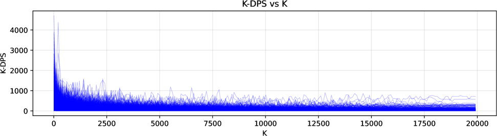
Figure 1: Effect of sampling size $K$ on the values of decision potential function, with each blue point representing the $K$-DPS value for a single input sample. Each blue line represents a trend of $K$-DPS for one input sample.

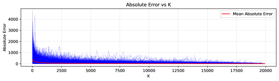
Figure 2: Effect of sampling size $K$ on the absolute error between the reference $K$-DPS (computed with $K=20,000$) and $K$-DPS values for varying $K$. Each blue line represents a trend of absolute error across input samples.

5.2 Influence of Sampling Grain $K$

We first evaluate the impact of the key hyperparameter, the sampling grain $K$, on the $K$-DPS value and the absolute errors between $K$-DPS and the ideal DPS. Specifically, we set $K=20,000$, a sufficiently large value, to simulate and approximate the ideal DPS. We then compute the $K$-DPS values by varying $K$ from 10 to 20,000 to illustrate how the decision potential value $\Phi_{f}^{K}(\cdot)$ converges to the ideal potential $\Phi_{f}^{\infty}(\cdot)$. Similarly, we calculate the absolute errors of $\Phi_{f}^{K}(\cdot)$ across different settings of $K$. As shown in Figure 1, the potential values rapidly converge to their true values (represented by horizontal lines at the tails), indicating that a relatively small $K$ can yield a highly accurate decision potential surface. Moreover, by examining the errors defined in Equation 8, as depicted in Figure 2, we observe that both the absolute error for individual samples and the empirically average error decrease to zero, confirming the effectiveness of $K$-DPS. Figures 1 and 2 also serve as valuable references for selecting appropriate $K$ values.

5.3 Empirical Concentration Bias

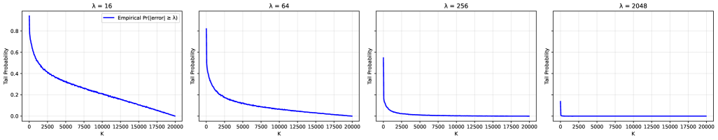
Figure 3: Empirical concentration experiments with different $\lambda$ values.

We also present an empirical study of concentration experiments, focusing on the trend of sample probabilities for inputs with a decision potential error exceeding a given fixed value $\lambda$ across various sampling sizes $K$. As shown in Figure 3, we evaluate the tail probability for $K$ values ranging from 10 to 20,000, with $\lambda$ set to 16, 64, 256, and 2048. These $\lambda$ values represent the geometric errors between the approximate and ideal DPS values. It is noteworthy to emphasize that even a $\lambda$ value of 256 is not excessively large or insignificant, as our decision potential function $\Phi_{f}^{K}(\cdot)$ is defined as the square of logarithmic errors, as specified in Equation 7.

From Figure 3, we observe that the tail probabilities exhibit an exponential decrease, indicating that the likelihood of exceeding a given error bound diminishes significantly with a linear increase in the sampling size $K$. Specifically, Figure 3 demonstrates that a sampling size of 10,000 ensures an absolute error below 64 with 90% confidence and an error below 256 with 99% probability. These results align closely with our absolute error analysis presented in Figure 2.

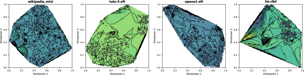
Figure 4: Contour visualization of the $K$-DPS ($K=2,500$) for Llama-3.2-1B on four datasets. Region colors represent the decision potential values. Black lines denote isohypses, with the 0-isohypse indicating decision boundary. Cubic interpolation is applied to construct the mesh grid, with visualizations using linear and nearest interpolation shown in Figures 6 and 7.

5.4 Visualizing Decision Potential Surface

While this paper primarily focuses on the error analysis of LLMs’ decision boundary construction, our proposed $K$-DPS can also be used to intuitively visualize both the decision boundary and the decision potential surface of an LLM under a given input distribution, as detailed in this section.

Settings. For visualization, we construct a low-dimensional representation of the original input distribution $\mathcal{D}^{\prime}$, typically in two dimensions to facilitate human understanding. First, we extract the last hidden state of an input $\mathbf{x}$ from the LLM as the original embedding of the input point. Next, we apply UMAP with 100 neighbors and a minimum distance of 0.2 for dimensionality reduction. Finally, we normalize the reduced embeddings to the range $[0,1]$ to construct the decision potential surface visualization. For interpolation, we evaluate nearest, linear, and cubic interpolation methods to approximate the $K$-DPS values on a mesh grid.

Visualization Results. As shown in Figure 4, we visualize the decision potential surface of the pretrained Llama-3.2-1B model on four corpora: Wikipedia Mini, Tulu-3-SFT, OpenO1-SFT, and HH-RLHF, using cubic interpolation. The heights of the isohypses are marked in the figures. The sampling size of $K=2,500$. From Figure 4, it is evident that most contours are at zero height, indicating that $K$-DPS effectively captures the decision boundary of large language models. Consequently, properties of the decision boundary (i.e., the 0-isohypse), such as curvature, location, and density, can be readily analyzed to facilitate interpretation and analysis of LLMs for future studies.

However, due to limitations in the interpolation strategy, the decision potential surface may be invalid in regions with sparse input points. For instance, the top-left regions of the second and fourth subfigures show $\Phi^{K}$ values significantly below zero, reflecting interpolation errors due to the absence of input samples in these areas. Additional visualizations with other interpolation methods are provided in the Appendix C for reference.

6 Conclusion

In this study, we explore the construction of decision boundaries for large language models. We identify the primary challenges as stemming from the expansive vocabulary size and the exponential growth in generated token sequences. To overcome these obstacles, we propose the concept of decision potential surface to quantify the confidence of language models in their decisions. We theoretically demonstrate that the zero-height isohypse on this surface corresponds to the decision boundary, and its approximated implementation substantially reduces the computational complexity of constructing the decision boundary. Through rigorous theoretical and empirical analyses, we evaluate the errors and validate the effectiveness of the proposed method.

Reproducibility Statement

As a theoretical study, we have clearly articulated all assumptions, definitions, theorems, and proofs in the main text and the Appendix. For the empirical results, we have provided the source code  to facilitate straightforward reproduction of the experimental findings. We welcome any additional suggestions to enhance the reproducibility of this work.

Appendix A LLM Usage

It is used for error checking, proofreading, result visualization, and code optimization.

Appendix B Proofs

B.1 Proof of Theorem 3.2

Proof.

Part I: Proof of Equation 2.

We aim to characterize the decision boundary $\mathcal{B}_{M}^{(f,\mathcal{D})}$ for a neural network $f:\mathbb{R}^{d}\to\mathbb{R}^{M}$ in the multi-class classification setting ($M>2$) under an input distribution $\mathcal{D}\subseteq\mathbb{R}^{d}$. The network is decomposed as $f=\sigma\circ f_{\text{cls}}\circ f_{r}$, where:

• $f_{r}:\mathbb{R}^{d}\to\mathbb{R}^{d_{h}}$ maps the input $\mathbf{x}$ to a latent representation $h=f_{r}(\mathbf{x})$,

• $f_{\text{cls}}:\mathbb{R}^{d_{h}}\to\mathbb{R}^{M}$ is a linear classification head, $f_{\text{cls}}(h)=W_{\text{cls}}h+b_{\text{cls}}$, with $W_{\text{cls}}\in\mathbb{R}^{M\times d_{h}}$, $b_{\text{cls}}\in\mathbb{R}^{M}$,

• $\sigma:\mathbb{R}^{M}\to\mathbb{R}^{M}$ is the softmax function, $\sigma(z)_{i}=\frac{e^{z_{i}}}{\sum_{j=1}^{M}e^{z_{j}}}$, producing probabilities $P=[p_{1},p_{2},\dots,p_{M}]$ with $\sum_{i=1}^{M}p_{i}=1$.

By Definition 3.1, the decision boundary $\mathcal{B}_{M}^{(f,\mathcal{D})}$ is the set of inputs $\mathbf{x}\in\mathcal{D}$ such that there exist at least two classes $m,n\in\mathcal{M}=\{1,2,\dots,M\}$, $m\neq n$, with equal and maximal probabilities:

$$p_{m}=p_{n}\geq\max_{o\in\mathcal{M}\setminus\{m,n\}}p_{o}.$$ (11)

Since $\sigma$ is the softmax function, $p_{m}=\sigma(z)_{m}=\frac{e^{z_{m}}}{\sum_{j=1}^{M}e^{z_{j}}}$, the condition $p_{m}=p_{n}$ implies:

$$\frac{e^{z_{m}}}{\sum_{j=1}^{M}e^{z_{j}}}=\frac{e^{z_{n}}}{\sum_{j=1}^{M}e^{z_{j}}}\implies e^{z_{m}}=e^{z_{n}}\implies z_{m}=z_{n}.$$ (12)

The logits are given by $z=W_{\text{cls}}h+b_{\text{cls}}$, so:

$$z_{m}=w_{m}h+b_{m},\quad z_{n}=w_{n}h+b_{n},$$ (13)

where $w_{m},w_{n}$ are the $m$-th and $n$-th rows of $W_{\text{cls}}$, and $b_{m},b_{n}$ are the corresponding entries of $b_{\text{cls}}$. Thus, $z_{m}=z_{n}$ implies:

$$(w_{m}-w_{n})h+(b_{m}-b_{n})=0.$$ (14)

Additionally, for $p_{m}=p_{n}$ to be maximal, we require $p_{m}\geq p_{o}$ for all $o\neq m,n$, which implies:

$$\frac{e^{z_{m}}}{\sum_{j=1}^{M}e^{z_{j}}}\geq\frac{e^{z_{o}}}{\sum_{j=1}^{M}e^{z_{j}}}\implies e^{z_{m}}\geq e^{z_{o}}\implies z_{m}\geq z_{o},\quad\forall o\neq m,n.$$ (15)

Since $z_{m}=z_{n}$, this becomes:

$$z_{m}=z_{n}\geq z_{o},\quad\forall o\neq m,n.$$ (16)

In the representation space, this translates to:

$$(w_{m}-w_{o})h+(b_{m}-b_{o})\geq 0,\quad(w_{n}-w_{o})h+(b_{n}-b_{o})\geq 0,\quad\forall o\neq m,n.$$ (17)

For each pair $m,n\in\mathcal{M}$, $1\leq m<n\leq M$, define:

$$\mathcal{B}_{mn}=\left\{h\in\mathbb{R}^{d_{h}}\mid(w_{m}-w_{n})h+(b_{m}-b_{n})=0,\,z_{m}=z_{n}\geq z_{o}\,\forall o\neq m,n,\,h=f_{r}(\mathbf{x}),\,\mathbf{x}\in\mathcal{D}\right\}.$$ (18)

The decision boundary is the union of all such pairwise boundaries:

$$\mathcal{B}_{M}^{(f,\mathcal{D})}=\bigcup_{1\leq m<n\leq M}\mathcal{B}_{mn}.$$ (19)

Part II: Voronoi Cells.

Each $\mathcal{B}_{mn}$ is a $(d_{h}-1)$-dimensional hyperplane in $\mathbb{R}^{d_{h}}$ defined by $(w_{m}-w_{n})h+(b_{m}-b_{n})=0$, restricted to points where $z_{m}=z_{n}\geq z_{o}$. Geometrically, the classification region for class $i$ is:

$$\mathcal{R}_{i}=\left\{h\in\mathbb{R}^{d_{h}}\mid w_{i}h+b_{i}>w_{j}h+b_{j},\,\forall j\neq i,\,h=f_{r}(\mathbf{x}),\,\mathbf{x}\in\mathcal{D}\right\}.$$ (20)

These regions are convex polytopes, as they are defined by the intersection of half-spaces $(w_{i}-w_{j})h+(b_{i}-b_{j})>0$. The boundaries between $\mathcal{R}_{m}$ and $\mathcal{R}_{n}$ occur where $(w_{m}-w_{n})h+(b_{m}-b_{n})=0$ and $z_{m}=z_{n}\geq z_{o}$, forming $\mathcal{B}_{mn}$. The collection $\{\mathcal{R}_{i}\}_{i=1}^{M}$ partitions the representation space, and the hyperplanes $\mathcal{B}_{mn}$ form the boundaries of a Voronoi-like partition, where each $\mathcal{R}_{i}$ is a Voronoi cell corresponding to class $i$.

This completes the proof. ∎

B.2 Proof of Theorem 3.3

Proof.

We aim to characterize the decision boundary $\mathcal{B}_{llm}^{(f,\mathcal{D}^{\prime})}$ of an LLM $f:\mathcal{V}^{N_{q}}\to\mathcal{V}^{N_{r}}$ under an input text distribution $\mathcal{D}^{\prime}\subseteq\bigcup_{n_{q}=1}^{N_{q}}\mathcal{V}^{n_{q}}$. The LLM generates a sequence $\mathbf{y}=[y_{1},\dots,y_{N_{r}}]\in\mathcal{V}^{N_{r}}$, where $\mathcal{V}=\{1,2,\dots,V\}$ is the vocabulary, conditioned on a prompt $\mathbf{x}\in\mathcal{D}^{\prime}$. The joint probability of generating $\mathbf{y}$ is:

$$P_{f}(\mathbf{y}|\mathbf{x})=\prod_{t=1}^{N_{r}}P_{f}(y_{t}|\mathbf{x},y_{1},\dots,y_{t-1}),$$

where $P_{f}(y_{t}|\mathbf{x},y_{1},\dots,y_{t-1})$ is the probability of predicting token $y_{t}$ at step $t$, modeled as a multi-class classification over $\mathcal{V}$.

Based on $\mathbf{y}^{*}=\arg\max_{\mathbf{y}\in\mathcal{V}^{N_{r}}}P_{f}(\mathbf{y}|\mathbf{x})$ and Definition 3.1, the decision boundary $\mathcal{B}_{llm}^{(f,\mathcal{D}^{\prime})}$ is the set of prompts $\mathbf{x}\in\mathcal{D}^{\prime}$ where at least two distinct sequences $\mathbf{y}_{v},\mathbf{y}_{w}\in\mathcal{V}^{N_{r}}$ have equal and maximal joint probabilities:

$$P_{f}(\mathbf{y}_{v}|\mathbf{x})=P_{f}(\mathbf{y}_{w}|\mathbf{x})\geq\max_{\mathbf{y}_{u}\in\mathcal{V}^{N_{r}}\setminus\{\mathbf{y}_{v},\mathbf{y}_{w}\}}P_{f}(\mathbf{y}_{u}|\mathbf{x}).$$

For each pair of distinct sequences $\mathbf{y}_{v},\mathbf{y}_{w}\in\mathcal{V}^{N_{r}}$, define:

$$\mathcal{B}_{llm,vw}=\left\{\mathbf{x}\in\mathcal{D}^{\prime}\mid P_{f}(\mathbf{y}_{v}|\mathbf{x})=P_{f}(\mathbf{y}_{w}|\mathbf{x})\geq\max_{\mathbf{y}_{u}\in\mathcal{V}^{N_{r}}\setminus\{\mathbf{y}_{v},\mathbf{y}_{w}\}}P_{f}(\mathbf{y}_{u}|\mathbf{x})\right\}.$$

The decision boundary is the union over all such pairs:

$$\mathcal{B}_{llm}^{(f,\mathcal{D}^{\prime})}=\bigcup_{\mathbf{y}_{v}\neq\mathbf{y}_{w}\in\mathcal{V}^{N_{r}}}\mathcal{B}_{llm,vw}.$$

To show this, consider the autoregressive process. For a prompt $\mathbf{x}$, the probability $P_{f}(\mathbf{y}|\mathbf{x})$ depends on the token probabilities at each step. Obviously, the predicted sequence $\mathbf{y}^{*}$ maximizes $P_{f}(\mathbf{y}|\mathbf{x})$. The decision boundary occurs when two sequences $\mathbf{y}_{v}$ and $\mathbf{y}_{w}$ have equal probabilities, and no other sequence has a higher probability. This implies:

$$P_{f}(\mathbf{y}_{v}|\mathbf{x})=\prod_{t=1}^{N_{r}}P_{f}(y_{v,t}|\mathbf{x},y_{v,1},\dots,y_{v,t-1})=\prod_{t=1}^{N_{r}}P_{f}(y_{w,t}|\mathbf{x},y_{w,1},\dots,y_{w,t-1})=P_{f}(\mathbf{y}_{w}|\mathbf{x}),$$

and for all $\mathbf{y}_{u}\neq\mathbf{y}_{v},\mathbf{y}_{w}$:

$$P_{f}(\mathbf{y}_{v}|\mathbf{x})\geq P_{f}(\mathbf{y}_{u}|\mathbf{x}).$$

Since each token prediction is a multi-class classification (as in Theorem 3.2), the boundary for a single token $y_{t}$ is defined by equal probabilities for the top tokens. For the full sequence, the boundary $\mathcal{B}_{llm,vw}$ corresponds to prompts $\mathbf{x}$ where the joint probabilities align, which may occur when the log-probabilities differ at some steps but sum to the same value. The maximality condition ensures that $\mathbf{y}_{v}$ and $\mathbf{y}_{w}$ are the top sequences.

This completes the proof. ∎

B.3 Proof of Theorem 4.3

Proof.

We aim to prove that the decision boundary $\mathcal{B}_{llm}^{(f,\mathcal{D}^{\prime})}$ defined in Theorem 3.3 is equivalent to the 0-isohypse $\mathcal{D}^{\prime}_{(0,f)}$ on the decision potential surface $\mathcal{S}^{(f,\mathcal{D}^{\prime})}$, and that the regions separated by this boundary correspond exactly to the Voronoi cells in the token-combined classification definition.

Recall from Theorem 3.3 that the decision boundary is

$$\mathcal{B}_{llm}^{(f,\mathcal{D}^{\prime})}=\bigcup_{\mathbf{y}_{v}\neq\mathbf{y}_{w}\in\mathcal{V}^{N_{r}}}\mathcal{B}_{llm,vw},$$ (21)

where

$$\mathcal{B}_{llm,vw}=\left\{\mathbf{x}\in\mathcal{D}^{\prime}\mid P_{f}(\mathbf{y}_{v}|\mathbf{x})=P_{f}(\mathbf{y}_{w}|\mathbf{x})\geq\max_{\mathbf{y}_{u}\in\mathcal{V}^{N_{r}}\setminus\{\mathbf{y}_{v},\mathbf{y}_{w}\}}P_{f}(\mathbf{y}_{u}|\mathbf{x})\right\}.$$ (22)

This boundary consists of prompts $\mathbf{x}$ where at least two distinct sequences $\mathbf{y}_{v}$ and $\mathbf{y}_{w}$ have equal and maximal joint probabilities, leading to ambiguity in the predicted output sequence.

From Definition 4.1, the decision potential function is

$$\Phi_{f}^{\infty}(\mathbf{x})=\left(\log P_{f}(\mathbf{y}_{1}|\mathbf{x})-\log P_{f}(\mathbf{y}_{2}|\mathbf{x})\right)^{2},$$ (23)

where $\mathbf{y}_{1},\mathbf{y}_{2}\in\mathcal{V}^{N_{r}}$ are the sequences with the highest and second-highest log-likelihoods, respectively. The 0-isohypse is defined as

$$\mathcal{D}^{\prime}_{(0,f)}=\left\{\mathbf{x}\in\mathcal{D}^{\prime}\mid\Phi_{f}^{\infty}(\mathbf{x})=0\right\}.$$ (24)

By definition, $\Phi_{f}^{\infty}(\mathbf{x})=0$ if and only if $\log P_{f}(\mathbf{y}_{1}|\mathbf{x})=\log P_{f}(\mathbf{y}_{2}|\mathbf{x})$, which implies $P_{f}(\mathbf{y}_{1}|\mathbf{x})=P_{f}(\mathbf{y}_{2}|\mathbf{x})$. Since $\mathbf{y}_{1}$ and $\mathbf{y}_{2}$ are the top two sequences by log-likelihood, this equality ensures that

$$P_{f}(\mathbf{y}_{1}|\mathbf{x})=P_{f}(\mathbf{y}_{2}|\mathbf{x})\geq P_{f}(\mathbf{y}_{u}|\mathbf{x}),\quad\forall\mathbf{y}_{u}\neq\mathbf{y}_{1},\mathbf{y}_{2},$$ (25)

satisfying the maximality condition in Theorem 3.3. Thus, $\mathbf{x}\in\mathcal{D}^{\prime}_{(0,f)}$ if and only if $\mathbf{x}\in\mathcal{B}_{llm}^{(f,\mathcal{D}^{\prime})}$, establishing the set equivalence

$$\mathcal{B}_{llm}^{(f,\mathcal{D}^{\prime})}=\mathcal{D}^{\prime}_{(0,f)}.$$ (26)

Geometrically, the regions separated by the 0-isohypse are the connected components of $\mathcal{D}^{\prime}\setminus\mathcal{D}^{\prime}_{(0,f)}$, where each region corresponds to prompts for which a unique sequence $\mathbf{y}_{i}$ has the highest log-likelihood ($\Phi_{f}^{\infty}(\mathbf{x})>0$). These regions are exactly the Voronoi cells in the sequence-level classification framework of Theorem 3.3, as each cell consists of prompts yielding the same maximal sequence. The 0-isohypse forms the boundaries between these cells, partitioning the prompt space $\mathcal{D}^{\prime}$ into regions of unambiguous predictions.

This completes the proof. ∎

B.4 Proof of Corollary 4.4

Proof.

We aim to show that for any $\varepsilon>0$, the input space $\mathcal{D}^{\prime}$ is partitioned into three disjoint strata based on the value of the decision potential function $\Phi_{f}^{\infty}(\mathbf{x})$:

$$\mathcal{D}^{\prime}=\mathcal{D}^{\prime}_{(>\varepsilon,f)}\sqcup\mathcal{D}^{\prime}_{(<\varepsilon,f)}\sqcup\mathcal{D}^{\prime}_{(\varepsilon,f)},$$ (27)

where $\sqcup$ denotes disjoint union.

From Definition 4.2, the $\varepsilon$-isohypse is

$$\mathcal{D}^{\prime}_{(\varepsilon,f)}=\left\{\mathbf{x}\in\mathcal{D}^{\prime}\mid\Phi_{f}^{\infty}(\mathbf{x})=\varepsilon\right\},$$ (28)

and the other strata are defined as

$$\mathcal{D}^{\prime}_{(>\varepsilon,f)}=\left\{\mathbf{x}\in\mathcal{D}^{\prime}\mid\Phi_{f}^{\infty}(\mathbf{x})>\varepsilon\right\},\quad\mathcal{D}^{\prime}_{(<\varepsilon,f)}=\left\{\mathbf{x}\in\mathcal{D}^{\prime}\mid\Phi_{f}^{\infty}(\mathbf{x})<\varepsilon\right\}.$$ (29)

Since $\Phi_{f}^{\infty}:\mathcal{D}^{\prime}\to\mathbb{R}_{+}$ is a continuous function (assuming log-likelihoods are continuous in the prompt space), these sets are disjoint and their union covers $\mathcal{D}^{\prime}$.

$\bullet$ $\varepsilon$-confident regions: For $\mathbf{x}\in\mathcal{D}^{\prime}_{(>\varepsilon,f)}$, $\Phi_{f}^{\infty}(\mathbf{x})>\varepsilon$, so

$$\left|\log P_{f}(\mathbf{y}_{1}|\mathbf{x})-\log P_{f}(\mathbf{y}_{2}|\mathbf{x})\right|>\sqrt{\varepsilon}.$$ (30)

Since $\mathbf{y}_{1}$ has the highest log-likelihood, $\log P_{f}(\mathbf{y}_{1}|\mathbf{x})-\log P_{f}(\mathbf{y}_{2}|\mathbf{x})>\sqrt{\varepsilon}$, meaning the model predicts $\mathbf{y}_{1}$ with at least $\sqrt{\varepsilon}$ nats (natural units of information) of confidence over the next most likely sequence $\mathbf{y}_{2}$.

$\bullet$ $\varepsilon$-uncertain regions: For $\mathbf{x}\in\mathcal{D}^{\prime}_{(<\varepsilon,f)}$, $\Phi_{f}^{\infty}(\mathbf{x})<\varepsilon$, so

$$\left|\log P_{f}(\mathbf{y}_{1}|\mathbf{x})-\log P_{f}(\mathbf{y}_{2}|\mathbf{x})\right|<\sqrt{\varepsilon}.$$ (31)

Here, the model has low confidence, with a margin less than $\sqrt{\varepsilon}$ nats between the top two sequences. As $\varepsilon\to 0$, $\Phi_{f}^{\infty}(\mathbf{x})\to 0$, so $\mathcal{D}^{\prime}_{(<\varepsilon,f)}$ converges to the 0-isohypse $\mathcal{D}^{\prime}_{(0,f)}$, where the margin is zero.

$\bullet$ $\varepsilon$-isohypse: For $\mathbf{x}\in\mathcal{D}^{\prime}_{(\varepsilon,f)}$, $\Phi_{f}^{\infty}(\mathbf{x})=\varepsilon$, so the confidence margin is exactly $\sqrt{\varepsilon}$ nats, forming the contour that separates confident and uncertain regions.

The disjointness of the strata follows from the strict inequalities and equality defining them, and their union covers $\mathcal{D}^{\prime}$ since $\Phi_{f}^{\infty}(\mathbf{x})\geq 0$ for all $\mathbf{x}\in\mathcal{D}^{\prime}$.

This completes the proof. ∎

B.5 Proof of Theorem 4.6

Proof.

Let $\mathbf{x}\in\mathcal{D}^{\prime}$ be a fixed input, and let $\mathcal{Y}_{K}=\{\mathbf{y}_{1},\mathbf{y}_{2},\dots,\mathbf{y}_{K}\}$ be a set of $K$ i.i.d. samples drawn from the language model’s output distribution $P_{f}(\cdot|\mathbf{x})$. The decision potential function is:

$$\Phi_{f}^{\infty}(\mathbf{x})=\left(\log P_{f}(\mathbf{y}_{1*}|\mathbf{x})-\log P_{f}(\mathbf{y}_{2*}|\mathbf{x})\right)^{2},$$ (32)

where $\mathbf{y}_{1*}$ and $\mathbf{y}_{2*}$ are the top-2 generated texts with the highest logarithmic likelihoods over the entire output space $\mathcal{V}^{N_{r}}$, and

$$\Phi_{f}^{K}(\mathbf{x})=\left(\log P_{f}(\mathbf{y}_{1*}^{K}|\mathbf{x})-\log P_{f}(\mathbf{y}_{2*}^{K}|\mathbf{x})\right)^{2},$$ (33)

where $\mathbf{y}_{1*}^{K}$ and $\mathbf{y}_{2*}^{K}$ are the top-2 generated texts within $\mathcal{Y}_{K}$. We aim to bound the error $|\Phi_{f}^{K}(\mathbf{x})-\Phi_{f}^{\infty}(\mathbf{x})|$ with probability at least $1-\delta-2\varepsilon_{\text{tail}}$ for $\delta\in(0,1)$.

Step 1: Preliminary. Define:

$$\Delta_{\infty}(\mathbf{x})=\log P_{f}(\mathbf{y}_{1*}|\mathbf{x})-\log P_{f}(\mathbf{y}_{2*}|\mathbf{x}),$$ (34)

$$\Delta_{K}(\mathbf{x})=\log P_{f}(\mathbf{y}_{1*}^{K}|\mathbf{x})-\log P_{f}(\mathbf{y}_{2*}^{K}|\mathbf{x}).$$

Thus, $\Phi_{f}^{\infty}(\mathbf{x})=(\Delta_{\infty}(\mathbf{x}))^{2}$ and $\Phi_{f}^{K}(\mathbf{x})=(\Delta_{K}(\mathbf{x}))^{2}$. The error can be expressed as:

$$|\Phi_{f}^{K}(\mathbf{x})-\Phi_{f}^{\infty}(\mathbf{x})| =|(\Delta_{K}(\mathbf{x}))^{2}-(\Delta_{\infty}(\mathbf{x}))^{2}|$$ (35)

$$=|\Delta_{K}(\mathbf{x})-\Delta_{\infty}(\mathbf{x})|\cdot|\Delta_{K}(\mathbf{x})+\Delta_{\infty}(\mathbf{x})|.$$

Since $\mathcal{Y}_{K}$ is a finite, $\mathbf{y}_{1*}^{K}$ and $\mathbf{y}_{2*}^{K}$ are the top-2 outputs in $\mathcal{Y}_{K}$, which may not include $\mathbf{y}_{1*}$ or $\mathbf{y}_{2*}$. Define:

$$R_{K}(\mathbf{x})=\log P_{f}(\mathbf{y}_{1*}^{K}|\mathbf{x})-\min_{\mathbf{y}\in\mathcal{Y}_{K}}\log P_{f}(\mathbf{y}|\mathbf{x}),$$ (36)

which represents the diameter of log-likelihoods in $\mathcal{Y}_{K}$.

Lemma B.1 ($\Pr(\mathbf{y}_{1*}\notin\mathcal{Y}_{K}))\leq\varepsilon_{\text{tail}}$).

Define the tail probability $\varepsilon_{\text{tail}}$ as: $\varepsilon_{\text{tail}}=\left(1-P_{f}(\mathbf{y}_{1*}^{K}|\mathbf{x})\right)^{K}$. Then, we have $\Pr(\mathbf{y}_{1*}\notin\mathcal{Y}_{K}))\leq\varepsilon_{\text{tail}}$,

A short proof of Lemma B.1: As $\mathbf{y}_{k}\in\mathcal{Y}_{K}$ are i.i.d., we know that with $K$-time sampling of $\mathbf{y}\sim P_{f}(\cdot|\mathbf{x})$ the probability that we cannot obtain $y_{1*}$ obeys a geometric distribution, i.e.,

$$\Pr(\mathbf{y}_{1*}\notin\mathcal{Y}_{k})=(1-P_{f}(\mathbf{y}_{1*}|\mathbf{x}))^{K}.$$ (37)

As $P_{f}(\mathbf{y}_{1*}|\mathbf{x})\geq P_{f}(\mathbf{y}_{1*}^{K}|\mathbf{x})$, then we have

$$\Pr(\mathbf{y}_{1*}\notin\mathcal{Y}_{K}))=(1-P_{f}(\mathbf{y}_{1*}|\mathbf{x}))^{K}\leq(1-P_{f}(\mathbf{y}_{1*}^{K}|\mathbf{x}))^{K}=\varepsilon_{\text{tail}},$$ (38)

which ends the proof.

Based on Lemma B.1, we know that $\varepsilon_{\text{tail}}$ bounds the probability that the true top output $\mathbf{y}_{1*}$ is not included in $\mathcal{Y}_{K}$.

Step 2: Bounding $|\Delta_{K}(\mathbf{x})-\Delta_{\infty}(\mathbf{x})|$.

Since $\Delta_{K}(\mathbf{x})$ is computed over a random sample, we consider using concentration inequalities to bound the deviation $|\Delta_{K}(\mathbf{x})-\Delta_{\infty}(\mathbf{x})|$. The log-likelihoods $\log P_{f}(\mathbf{y}_{k}|\mathbf{x})$ for $\mathbf{y}_{k}\in\mathcal{Y}_{K}$ are i.i.d., and they are bounded within the diameter $R_{K}(\mathbf{x})$. By Hoeffding’s inequality, the deviation of the sample maximum log-likelihood from its expected maximum is bounded. Specifically, for the top-1 log-likelihood $\forall~t>0$, we have:

$$\Pr\left(\left|\log P_{f}(\mathbf{y}_{1*}^{K}|\mathbf{x})-\log P_{f}(\mathbf{y}_{1*}|\mathbf{x})\right|>t\right)\leq 2\exp\left(-\frac{2Kt^{2}}{R_{K}^{2}(\mathbf{x})}\right).$$ (39)

Similarly, for the second-highest log-likelihood, a similar bound applies.

Combining these, we have:

$$|\Delta_{K}(\mathbf{x})-\Delta_{\infty}(\mathbf{x})| =|\left(\log P_{f}(\mathbf{y}_{1*}^{K}|\mathbf{x})-\log P_{f}(\mathbf{y}_{2*}^{K}|\mathbf{x})\right)-\left(\log P_{f}(\mathbf{y}_{1*}|\mathbf{x})-\log P_{f}(\mathbf{y}_{2*}|\mathbf{x})\right)|$$ (40)

$$=|\left(\log P_{f}(\mathbf{y}_{1*}^{K}|\mathbf{x})-\log P_{f}(\mathbf{y}_{1*}|\mathbf{x})\right)-\left(\log P_{f}(\mathbf{y}_{2*}^{K}|\mathbf{x})-\log P_{f}(\mathbf{y}_{2*}|\mathbf{x})\right)|.$$

Based on the triangle inequality $|a-b|\leq|a|+|b|$ when $a,b\in\mathbb{R}$, we know that

$$|\Delta_{K}(\mathbf{x})-\Delta_{\infty}(\mathbf{x})| =|\left(\log P_{f}(\mathbf{y}_{1*}^{K}|\mathbf{x})-\log P_{f}(\mathbf{y}_{1*}|\mathbf{x})\right)-\left(\log P_{f}(\mathbf{y}_{2*}^{K}|\mathbf{x})-\log P_{f}(\mathbf{y}_{2*}|\mathbf{x})\right)|$$ (41)

$$\leq|\log P_{f}(\mathbf{y}_{1*}^{K}|\mathbf{x})-\log P_{f}(\mathbf{y}_{1*}|\mathbf{x})|+|\log P_{f}(\mathbf{y}_{2*}^{K}|\mathbf{x})-\log P_{f}(\mathbf{y}_{2*}|\mathbf{x})|.$$

To bound $|\Delta_{K}(\mathbf{x})-\Delta_{\infty}(\mathbf{x})|$, we aim to find the maximal probability for the event $|\Delta_{K}(\mathbf{x})-\Delta_{\infty}(\mathbf{x})|<t^{\prime}$ with $t^{\prime}>0$. Without losing generality, we set $t^{\prime}=2t$, where the objective can be reformated as:

$$\Pr(|\Delta_{K}(\mathbf{x})-\Delta_{\infty}(\mathbf{x})|<t^{\prime})$$ (42)

$$=1-\Pr(|\Delta_{K}(\mathbf{x})-\Delta_{\infty}(\mathbf{x})|>=t^{\prime}),$$

where

$$\Pr(|\Delta_{K}(\mathbf{x})-\Delta_{\infty}(\mathbf{x})|>=t^{\prime})$$ (43)

$$=\Pr(|\log P_{f}(\mathbf{y}_{1*}^{K}|\mathbf{x})-\log P_{f}(\mathbf{y}_{1*}|\mathbf{x})|\geq t\mathbf{~or~}|\log P_{f}(\mathbf{y}_{2*}^{K}|\mathbf{x})-\log P_{f}(\mathbf{y}_{2*}|\mathbf{x})|\geq t))$$

$$\leq\Pr(|\log P_{f}(\mathbf{y}_{1*}^{K}|\mathbf{x})-\log P_{f}(\mathbf{y}_{1*}|\mathbf{x})|\geq t)+\Pr(|\log P_{f}(\mathbf{y}_{3*}^{K}|\mathbf{x})-\log P_{f}(\mathbf{y}_{2*}|\mathbf{x})|\geq t)$$

$$\leq 2\exp\left(-\frac{2Kt^{2}}{R_{K}^{2}(\mathbf{x})}\right)+2\exp\left(-\frac{2Kt^{2}}{R_{K}^{2}(\mathbf{x})}\right)$$

$$=4\exp\left(-\frac{2Kt^{2}}{R_{K}^{2}(\mathbf{x})}\right).$$

So we have

$$\Pr(|\Delta_{K}(\mathbf{x})-\Delta_{\infty}(\mathbf{x})|<t^{\prime})$$ (44)

$$=1-\Pr(|\Delta_{K}(\mathbf{x})-\Delta_{\infty}(\mathbf{x})|>=t^{\prime})$$

$$\geq 1-4\exp\left(-\frac{2Kt^{2}}{R_{K}^{2}(\mathbf{x})}\right).$$

Suppose we have at least $1-\delta$ probability to support this event stands, we have

$$~~~~~~1-4\exp\left(-\frac{2Kt^{2}}{R_{K}^{2}(\mathbf{x})}\right)\geq 1-\delta$$ (45)

$$\Leftrightarrow 4\exp\left(-\frac{2Kt^{2}}{R_{K}^{2}(\mathbf{x})}\right)\leq\delta$$

$$\Leftrightarrow\exp\left(-\frac{2Kt^{2}}{R_{K}^{2}(\mathbf{x})}\right)\leq\frac{\delta}{4}$$

$$\Leftrightarrow-\frac{2Kt^{2}}{R_{K}^{2}(\mathbf{x})}\leq\log\frac{\delta}{4}$$

$$\Leftrightarrow\frac{2Kt^{2}}{R_{K}^{2}(\mathbf{x})}\geq-\log\frac{\delta}{4}$$

$$\Leftrightarrow\frac{2Kt^{2}}{R_{K}^{2}(\mathbf{x})}\geq\log\frac{4}{\delta}$$

$$\Leftrightarrow t^{2}\geq\frac{R_{K}^{2}(\mathbf{x})}{2K}\log\frac{4}{\delta}$$

$$\Leftrightarrow t\geq|{R_{K}(\mathbf{x})}\sqrt{\frac{log(4/\delta)}{2K}}|$$

$$\Leftrightarrow t\geq{R_{K}(\mathbf{x})}\sqrt{\frac{log(4/\delta)}{2K}}.$$

In other words, $\forall~t>0$ we bound $\Pr(|\Delta_{K}(\mathbf{x})-\Delta_{\infty}(\mathbf{x})|<t)$ with probability at least $1-\delta$ when:

$$t=R_{K}(\mathbf{x})\sqrt{\frac{\log(4/\delta)}{2K}}.$$ (46)

Step 3: Bounding $|\Delta_{K}(\mathbf{x})+\Delta_{\infty}(\mathbf{x})|$.

Assumption B.2 (Bounded Population Gap).

There exists a constant $M>0$ such that for any $\mathbf{x}$, the population top-2 gap satisfies:

$$\Delta_{\infty}(\mathbf{x})=\log P_{f}(\mathbf{y}_{1*}|\mathbf{x})-\log P_{f}(\mathbf{y}_{2*}|\mathbf{x})\leq M$$ (47)

Then we assume that

$$M\leq R_{K}(\mathbf{x})$$ (48)

when $K\gg 1$.

This assumption is reasonable as most practical language models do not have extremely large differences between top-2 probabilities, and the probability differences between top-2 would be much smaller than the range of between the top-1 and the sample with the minimal probailitty in the sampling set. Now we can obtain that:

$$|\Delta_{K}(\mathbf{x})+\Delta_{\infty}(\mathbf{x})|\leq|\Delta_{K}(\mathbf{x})|+|\Delta_{\infty}(\mathbf{x})|\leq 2\cdot R_{K}(\mathbf{x}).$$ (49)

Step 4: Final bound.

Define the events

$$A=\{\mathbf{y}_{1*}\in\mathcal{Y}_{K}\text{ and }\mathbf{y}_{2*}\in\mathcal{Y}_{K}\},\qquad B=\{\mathbf{y}_{1*}\notin\mathcal{Y}_{K}\text{ or }\mathbf{y}_{2*}\notin\mathcal{Y}_{K}\}.$$ (50)

Lemma B.1 and a union bound give

$$\Pr(B)\leq 2\varepsilon_{\text{tail}}.$$ (51)

• On event $A$ we have $\mathbf{y}_{1*}^{K}=\mathbf{y}_{1*}$ and $\mathbf{y}_{2*}^{K}=\mathbf{y}_{2*}$, hence

  $$\Phi_{f}^{K}(\mathbf{x})=\Phi_{f}^{\infty}(\mathbf{x})\quad\Longrightarrow\quad|\Phi_{f}^{K}(\mathbf{x})-\Phi_{f}^{\infty}(\mathbf{x})|=0.$$ (52)

• On event $B$ we use the worst-case gap

  $$|\Phi_{f}^{K}(\mathbf{x})-\Phi_{f}^{\infty}(\mathbf{x})|$$ (53)

  $$\leq|\Delta_{K}(\mathbf{x})-\Delta_{\infty}(\mathbf{x})|\cdot|\Delta_{K}(\mathbf{x})+\Delta_{\infty}(\mathbf{x})|$$

  $$\leq R_{K}(\mathbf{x})\sqrt{\frac{\log(4/\delta)}{2K}}\cdot 2R_{K}(x)$$

  $$=2R_{K}^{2}(\mathbf{x})\sqrt{\frac{\log(4/\delta)}{2K}}.$$

This completes the proof. ∎

B.6 Proof of Theorem 4.7

Proof.

We aim to bound the expected error $\mathbb{E}[|\Phi_{f}^{K}(\mathbf{x})-\Phi_{f}^{\infty}(\mathbf{x})|]$ for a fixed input $\mathbf{x}\in\mathcal{D}^{\prime}$ and a set $\mathcal{Y}_{K}=\{\mathbf{y}_{1},\mathbf{y}_{2},\dots,\mathbf{y}_{K}\}$ of $K$ i.i.d. samples drawn from the language model’s output distribution $P_{f}(\cdot|\mathbf{x})$. Recall that:

$$\Phi_{f}^{\infty}(\mathbf{x})=\left(\log P_{f}(\mathbf{y}_{1*}|\mathbf{x})-\log P_{f}(\mathbf{y}_{2*}|\mathbf{x})\right)^{2},\quad\Phi_{f}^{K}(\mathbf{x})=\left(\log P_{f}(\mathbf{y}_{1*}^{K}|\mathbf{x})-\log P_{f}(\mathbf{y}_{2*}^{K}|\mathbf{x})\right)^{2},$$ (54)

where $\mathbf{y}_{1*},\mathbf{y}_{2*}$ are the top-2 outputs over the entire output space $\mathcal{V}^{N_{r}}$, and $\mathbf{y}_{1*}^{K},\mathbf{y}_{2*}^{K}$ are the top-2 outputs in $\mathcal{Y}_{K}$. Define:

$$\Delta_{\infty}(\mathbf{x})=\log P_{f}(\mathbf{y}_{1*}|\mathbf{x})-\log P_{f}(\mathbf{y}_{2*}|\mathbf{x}),\quad\Delta_{K}(\mathbf{x})=\log P_{f}(\mathbf{y}_{1*}^{K}|\mathbf{x})-\log P_{f}(\mathbf{y}_{2*}^{K}|\mathbf{x}),$$ (55)

so that $\Phi_{f}^{\infty}(\mathbf{x})=(\Delta_{\infty}(\mathbf{x}))^{2}$, $\Phi_{f}^{K}(\mathbf{x})=(\Delta_{K}(\mathbf{x}))^{2}$, and the error is:

$$|\Phi_{f}^{K}(\mathbf{x})-\Phi_{f}^{\infty}(\mathbf{x})|=|(\Delta_{K}(\mathbf{x}))^{2}-(\Delta_{\infty}(\mathbf{x}))^{2}|=|\Delta_{K}(\mathbf{x})-\Delta_{\infty}(\mathbf{x})|\cdot|\Delta_{K}(\mathbf{x})+\Delta_{\infty}(\mathbf{x})|.$$ (56)

By Assumption B.2, $|\Delta_{\infty}(\mathbf{x})|\leq R_{K}(\mathbf{x})$, where $R_{K}(\mathbf{x})=\log P_{f}(\mathbf{y}_{1*}^{K}|\mathbf{x})-\min_{\mathbf{y}\in\mathcal{Y}_{K}}\log P_{f}(\mathbf{y}|\mathbf{x})$ is the log-likelihood diameter of $\mathcal{Y}_{K}$. Also, $|\Delta_{K}(\mathbf{x})|\leq R_{K}(\mathbf{x})$, so:

$$|\Delta_{K}(\mathbf{x})+\Delta_{\infty}(\mathbf{x})|\leq|\Delta_{K}(\mathbf{x})|+|\Delta_{\infty}(\mathbf{x})|\leq 2R_{K}(\mathbf{x}).$$ (57)

Thus, the error is bounded by:

$$|\Phi_{f}^{K}(\mathbf{x})-\Phi_{f}^{\infty}(\mathbf{x})|\leq|\Delta_{K}(\mathbf{x})-\Delta_{\infty}(\mathbf{x})|\cdot 2R_{K}(\mathbf{x}).$$ (58)

We compute the expectation:

$$\mathbb{E}[|\Phi_{f}^{K}(\mathbf{x})-\Phi_{f}^{\infty}(\mathbf{x})|]\leq 2R_{K}(\mathbf{x})\cdot\mathbb{E}[|\Delta_{K}(\mathbf{x})-\Delta_{\infty}(\mathbf{x})|].$$ (59)

Define $Z=|\Delta_{K}(\mathbf{x})-\Delta_{\infty}(\mathbf{x})|$. From the proof of Theorem 4.6 (Equation 43), Hoeffding’s inequality gives:

$$\Pr(Z\geq t)\leq 4\exp\left(-\frac{2Kt^{2}}{R_{K}^{2}(\mathbf{x})}\right).$$ (60)

The expectation of $Z$ is:

$$\mathbb{E}[Z]=\int_{0}^{\infty}\Pr(Z\geq t)\,dt\leq\int_{0}^{\infty}4\exp\left(-\frac{2Kt^{2}}{R_{K}^{2}(\mathbf{x})}\right)\,dt.$$ (61)

Substitute $u=\frac{2Kt^{2}}{R_{K}^{2}(\mathbf{x})}$, so $t=R_{K}(\mathbf{x})\sqrt{\frac{u}{2K}}$, $dt=\frac{R_{K}(\mathbf{x})}{2\sqrt{2K}\sqrt{u}}\,du$. Then:

$$\mathbb{E}[Z]\leq\int_{0}^{\infty}4e^{-u}\cdot\frac{R_{K}(\mathbf{x})}{2\sqrt{2K}\sqrt{u}}\,du=\frac{2R_{K}(\mathbf{x})}{\sqrt{2K}}\int_{0}^{\infty}\frac{e^{-u}}{\sqrt{u}}\,du.$$ (62)

Since $\int_{0}^{\infty}\frac{e^{-u}}{\sqrt{u}}\,du=\Gamma\left(\frac{1}{2}\right)=\sqrt{\pi}$, we have:

$$\mathbb{E}[Z]\leq\frac{2R_{K}(\mathbf{x})}{\sqrt{2K}}\cdot\sqrt{\pi}=R_{K}(\mathbf{x})\sqrt{\frac{2\pi}{K}}.$$ (63)

Thus:

$$\mathbb{E}[|\Phi_{f}^{K}(\mathbf{x})-\Phi_{f}^{\infty}(\mathbf{x})|]\leq 2R_{K}(\mathbf{x})\cdot R_{K}(\mathbf{x})\sqrt{\frac{2\pi}{K}}=2R_{K}^{2}(\mathbf{x})\sqrt{\frac{2\pi}{K}}.$$ (64)

To account for event $B=\{\mathbf{y}_{1*}\notin\mathcal{Y}_{K}\text{ or }\mathbf{y}_{2*}\notin\mathcal{Y}_{K}\}$ with $\Pr(B)\leq 2\varepsilon_{\text{tail}}$ (from Lemma B.1 and union bound), we note that on event $A=\{\mathbf{y}_{1*}\in\mathcal{Y}_{K}\text{ and }\mathbf{y}_{2*}\in\mathcal{Y}_{K}\}$, the error is zero. Thus, we add a conservative term for event $B$, where the error is at most $2R_{K}^{2}(\mathbf{x})$ (since $|\Delta_{K}|,|\Delta_{\infty}|\leq R_{K}(\mathbf{x})$, so $|\Phi_{f}^{K}(\mathbf{x})-\Phi_{f}^{\infty}(\mathbf{x})|\leq 2R_{K}^{2}(\mathbf{x})$):

$$\mathbb{E}[|\Phi_{f}^{K}(\mathbf{x})-\Phi_{f}^{\infty}(\mathbf{x})|\cdot\mathds{1}_{B}]\leq 2R_{K}^{2}(\mathbf{x})\cdot\Pr(B)\leq 2R_{K}^{2}(\mathbf{x})\cdot 2\varepsilon_{\text{tail}}=4R_{K}^{2}(\mathbf{x})\varepsilon_{\text{tail}},$$ (65)

where $\mathds{1}_{B}$ is the indicator function which is $1$ only when event $B$ occurs.

Combining both terms, the expected error is:

$$\mathbb{E}[|\Phi_{f}^{K}(\mathbf{x})-\Phi_{f}^{\infty}(\mathbf{x})|]\leq 2R_{K}^{2}(\mathbf{x})\sqrt{\frac{2\pi}{K}}+4R_{K}^{2}(\mathbf{x})\varepsilon_{\text{tail}},$$ (66)

where $\varepsilon_{\text{tail}}=\left(1-P_{f}(\mathbf{y}_{1*}^{K}|\mathbf{x})\right)^{K}$. This completes the proof. ∎

B.7 Proof of Corollary 4.8

Proof.

We aim to bound the tail probability $\Pr(|\Phi_{f}^{K}(\mathbf{x})-\Phi_{f}^{\infty}(\mathbf{x})|\geq\lambda)$ for $\lambda>0$. Using the same notation as in Theorem 4.7, we have:

$$|\Phi_{f}^{K}(\mathbf{x})-\Phi_{f}^{\infty}(\mathbf{x})|=|\Delta_{K}(\mathbf{x})-\Delta_{\infty}(\mathbf{x})|\cdot|\Delta_{K}(\mathbf{x})+\Delta_{\infty}(\mathbf{x})|.$$ (67)

Since $|\Delta_{K}(\mathbf{x})+\Delta_{\infty}(\mathbf{x})|\leq 2R_{K}(\mathbf{x})$, let $Z=|\Delta_{K}(\mathbf{x})-\Delta_{\infty}(\mathbf{x})|$, so:

$$|\Phi_{f}^{K}(\mathbf{x})-\Phi_{f}^{\infty}(\mathbf{x})|\leq Z\cdot 2R_{K}(\mathbf{x}).$$ (68)

Thus:

$$\Pr(|\Phi_{f}^{K}(\mathbf{x})-\Phi_{f}^{\infty}(\mathbf{x})|\geq\lambda)=\Pr\left(Z\cdot 2R_{K}(\mathbf{x})\geq\lambda\right)=\Pr\left(Z\geq\frac{\lambda}{2R_{K}(\mathbf{x})}\right).$$ (69)

From the proof of Theorem 4.6 (Equation 43), Hoeffding’s inequality gives:

$$\Pr\left(Z\geq t\right)\leq 4\exp\left(-\frac{2Kt^{2}}{R_{K}^{2}(\mathbf{x})}\right).$$ (70)

Set $t=\frac{\lambda}{2R_{K}(\mathbf{x})}$:

$$\Pr\left(Z\geq\frac{\lambda}{2R_{K}(\mathbf{x})}\right)\leq 4\exp\left(-\frac{2K\cdot\left(\frac{\lambda}{2R_{K}(\mathbf{x})}\right)^{2}}{R_{K}^{2}(\mathbf{x})}\right)=4\exp\left(-\frac{K\lambda^{2}}{2R_{K}^{4}(\mathbf{x})}\right).$$ (71)

Define events $A=\{\mathbf{y}_{1*}\in\mathcal{Y}_{K}\text{ and }\mathbf{y}_{2*}\in\mathcal{Y}_{K}\}$ and $B=\{\mathbf{y}_{1*}\notin\mathcal{Y}_{K}\text{ or }\mathbf{y}_{2*}\notin\mathcal{Y}_{K}\}$. On event $A$, the error is zero, so it does not contribute to the tail probability. On event $B$, with $\Pr(B)\leq 2\varepsilon_{\text{tail}}$ (from Lemma B.1 and union bound), the tail probability is bounded by:

$$\Pr(|\Phi_{f}^{K}(\mathbf{x})-\Phi_{f}^{\infty}(\mathbf{x})|\geq\lambda)\leq\Pr\left(\left\{Z\geq\frac{\lambda}{2R_{K}(\mathbf{x})}\right\}\cap B\right)+\Pr(A).$$ (72)

Since $\Pr(A)\geq 1-2\varepsilon_{\text{tail}}$ and the error is zero on $A$, we focus on event $B$:

$$\Pr\left(\left\{Z\geq\frac{\lambda}{2R_{K}(\mathbf{x})}\right\}\cap B\right)\leq\Pr\left(Z\geq\frac{\lambda}{2R_{K}(\mathbf{x})}\right)+\Pr(B)\leq 4\exp\left(-\frac{K\lambda^{2}}{2R_{K}^{4}(\mathbf{x})}\right)+2\varepsilon_{\text{tail}}.$$ (73)

Thus, the tail probability is:

$$\Pr\left(|\Phi_{f}^{K}(\mathbf{x})-\Phi_{f}^{\infty}(\mathbf{x})|\geq\lambda\right)\leq 4\exp\left(-\frac{K\lambda^{2}}{2R_{K}^{4}(\mathbf{x})}\right)+2\varepsilon_{\text{tail}},$$ (74)

where $\varepsilon_{\text{tail}}=\left(1-P_{f}(\mathbf{y}_{1*}^{K}|\mathbf{x})\right)^{K}$. This completes the proof. ∎

Appendix C Supplemental Experiments

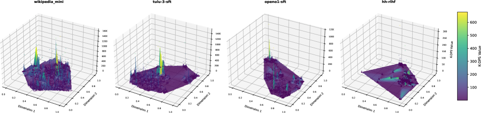
Figure 5: Three-dimensional visualization of the $K$-DPS ($K=2,500$) for Llama-3.2-1B on four datasets.

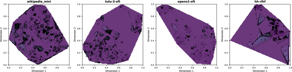
Figure 6: Contour visualization of 2,500-grained decision potential surface for Llama3.2-1B on four datasets with linear interpolation.

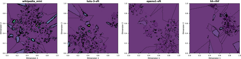
Figure 7: Contour visualization of 2,500-grained decision potential surface of Llama3.2-1B on four datasets with nearest interpolation.

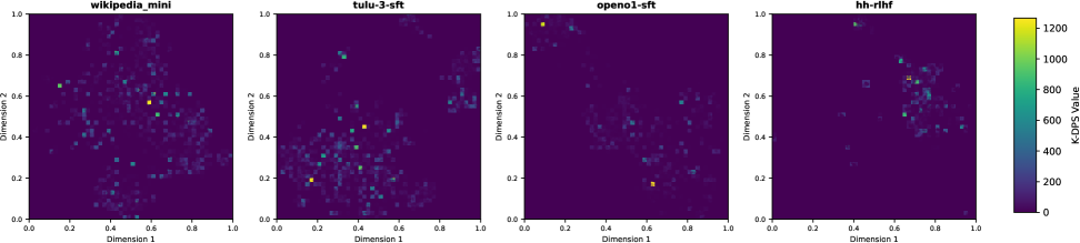
Figure 8: Heatmap visualization of the decision potential surface on Four datasets.

References

- Abdin et al. (2024) Marah Abdin, Jyoti Aneja, Harkirat Behl, Sébastien Bubeck, Ronen Eldan, Suriya Gunasekar, Michael Harrison, Russell J. Hewett, Mojan Javaheripi, Piero Kauffmann, James R. Lee, Yin Tat Lee, Yuanzhi Li, Weishung Liu, Caio C. T. Mendes, Anh Nguyen, Eric Price, Gustavo de Rosa, Olli Saarikivi, Adil Salim, Shital Shah, Xin Wang, Rachel Ward, Yue Wu, Dingli Yu, Cyril Zhang, and Yi Zhang. Phi-4 technical report, 2024. URL https://arxiv.org/abs/2412.08905.
- Allen-Zhu & Li (2023) Zeyuan Allen-Zhu and Yuanzhi Li. Physics of language models: Part 3.2, knowledge manipulation. arXiv preprint arXiv:2309.14402, 2023.
- Ameisen et al. (2025) Emmanuel Ameisen, Jack Lindsey, Adam Pearce, Wes Gurnee, Nicholas L Turner, Brian Chen, Craig Citro, David Abrahams, Shan Carter, Basil Hosmer, et al. Circuit tracing: Revealing computational graphs in language models. Transformer Circuits Thread, 6, 2025.
- Bengio et al. (2003) Yoshua Bengio, Réjean Ducharme, Pascal Vincent, and Christian Janvin. A neural probabilistic language model. J. Mach. Learn. Res., 3:1137–1155, 2003. URL https://jmlr.org/papers/v3/bengio03a.html.
- Conmy et al. (2023) Arthur Conmy, Augustine N. Mavor-Parker, Aengus Lynch, Stefan Heimersheim, and Adrià Garriga-Alonso. Towards automated circuit discovery for mechanistic interpretability. In Alice Oh, Tristan Naumann, Amir Globerson, Kate Saenko, Moritz Hardt, and Sergey Levine (eds.), Advances in Neural Information Processing Systems 36: Annual Conference on Neural Information Processing Systems 2023, NeurIPS 2023, New Orleans, LA, USA, December 10 - 16, 2023, 2023. URL http://papers.nips.cc/paper_files/paper/2023/hash/34e1dbe95d34d7ebaf99b9bcaeb5b2be-Abstract-Conference.html.
- Elhage et al. (2021) Nelson Elhage, Neel Nanda, Catherine Olsson, Tom Henighan, Nicholas Joseph, Ben Mann, Amanda Askell, Yuntao Bai, Anna Chen, Tom Conerly, et al. A mathematical framework for transformer circuits. Transformer Circuits Thread, 1(1):12, 2021.
- Ganguli et al. (2022) Deep Ganguli, Liane Lovitt, Jackson Kernion, Amanda Askell, Yuntao Bai, Saurav Kadavath, Ben Mann, Ethan Perez, Nicholas Schiefer, Kamal Ndousse, Andy Jones, Sam Bowman, Anna Chen, Tom Conerly, Nova DasSarma, Dawn Drain, Nelson Elhage, Sheer El-Showk, Stanislav Fort, Zac Hatfield-Dodds, Tom Henighan, Danny Hernandez, Tristan Hume, Josh Jacobson, Scott Johnston, Shauna Kravec, Catherine Olsson, Sam Ringer, Eli Tran-Johnson, Dario Amodei, Tom Brown, Nicholas Joseph, Sam McCandlish, Chris Olah, Jared Kaplan, and Jack Clark. Red teaming language models to reduce harms: Methods, scaling behaviors, and lessons learned, 2022. URL https://arxiv.org/abs/2209.07858.
- Goodfellow et al. (2015) Ian J. Goodfellow, Jonathon Shlens, and Christian Szegedy. Explaining and harnessing adversarial examples. In 3rd International Conference on Learning Representations (ICLR 2015), San Diego, CA, USA, 2015.
- Grattafiori et al. (2024) Aaron Grattafiori, Abhimanyu Dubey, Abhinav Jauhri, Abhinav Pandey, Abhishek Kadian, Ahmad Al-Dahle, Aiesha Letman, Akhil Mathur, Alan Schelten, Alex Vaughan, Amy Yang, Angela Fan, Anirudh Goyal, Anthony Hartshorn, Aobo Yang, Archi Mitra, Archie Sravankumar, Artem Korenev, Arthur Hinsvark, Arun Rao, Aston Zhang, Aurelien Rodriguez, Austen Gregerson, Ava Spataru, Baptiste Roziere, Bethany Biron, Binh Tang, Bobbie Chern, Charlotte Caucheteux, Chaya Nayak, Chloe Bi, Chris Marra, Chris McConnell, Christian Keller, Christophe Touret, Chunyang Wu, Corinne Wong, Cristian Canton Ferrer, Cyrus Nikolaidis, Damien Allonsius, Daniel Song, Danielle Pintz, Danny Livshits, Danny Wyatt, David Esiobu, Dhruv Choudhary, Dhruv Mahajan, Diego Garcia-Olano, Diego Perino, Dieuwke Hupkes, Egor Lakomkin, Ehab AlBadawy, Elina Lobanova, Emily Dinan, Eric Michael Smith, Filip Radenovic, Francisco Guzmán, Frank Zhang, Gabriel Synnaeve, Gabrielle Lee, Georgia Lewis Anderson, Govind Thattai, Graeme Nail, Gregoire Mialon, Guan Pang, Guillem Cucurell, Hailey Nguyen, Hannah Korevaar, Hu Xu, Hugo Touvron, Iliyan Zarov, Imanol Arrieta Ibarra, Isabel Kloumann, Ishan Misra, Ivan Evtimov, Jack Zhang, Jade Copet, Jaewon Lee, Jan Geffert, Jana Vranes, Jason Park, Jay Mahadeokar, Jeet Shah, Jelmer van der Linde, Jennifer Billock, Jenny Hong, Jenya Lee, Jeremy Fu, Jianfeng Chi, Jianyu Huang, Jiawen Liu, Jie Wang, Jiecao Yu, Joanna Bitton, Joe Spisak, Jongsoo Park, Joseph Rocca, Joshua Johnstun, Joshua Saxe, Junteng Jia, Kalyan Vasuden Alwala, Karthik Prasad, Kartikeya Upasani, Kate Plawiak, Ke Li, Kenneth Heafield, Kevin Stone, Khalid El-Arini, Krithika Iyer, Kshitiz Malik, Kuenley Chiu, Kunal Bhalla, Kushal Lakhotia, Lauren Rantala-Yeary, Laurens van der Maaten, Lawrence Chen, Liang Tan, Liz Jenkins, Louis Martin, Lovish Madaan, Lubo Malo, Lukas Blecher, Lukas Landzaat, Luke de Oliveira, Madeline Muzzi, Mahesh Pasupuleti, Mannat Singh, Manohar Paluri, Marcin Kardas, Maria Tsimpoukelli, Mathew Oldham, Mathieu Rita, Maya Pavlova, Melanie Kambadur, Mike Lewis, Min Si, Mitesh Kumar Singh, Mona Hassan, Naman Goyal, Narjes Torabi, Nikolay Bashlykov, Nikolay Bogoychev, Niladri Chatterji, Ning Zhang, Olivier Duchenne, Onur Çelebi, Patrick Alrassy, Pengchuan Zhang, Pengwei Li, Petar Vasic, Peter Weng, Prajjwal Bhargava, Pratik Dubal, Praveen Krishnan, Punit Singh Koura, Puxin Xu, Qing He, Qingxiao Dong, Ragavan Srinivasan, Raj Ganapathy, Ramon Calderer, Ricardo Silveira Cabral, Robert Stojnic, Roberta Raileanu, Rohan Maheswari, Rohit Girdhar, Rohit Patel, Romain Sauvestre, Ronnie Polidoro, Roshan Sumbaly, Ross Taylor, Ruan Silva, Rui Hou, Rui Wang, Saghar Hosseini, Sahana Chennabasappa, Sanjay Singh, Sean Bell, Seohyun Sonia Kim, Sergey Edunov, Shaoliang Nie, Sharan Narang, Sharath Raparthy, Sheng Shen, Shengye Wan, Shruti Bhosale, Shun Zhang, Simon Vandenhende, Soumya Batra, Spencer Whitman, Sten Sootla, Stephane Collot, Suchin Gururangan, Sydney Borodinsky, Tamar Herman, Tara Fowler, Tarek Sheasha, Thomas Georgiou, Thomas Scialom, Tobias Speckbacher, Todor Mihaylov, Tong Xiao, Ujjwal Karn, Vedanuj Goswami, Vibhor Gupta, Vignesh Ramanathan, Viktor Kerkez, Vincent Gonguet, Virginie Do, Vish Vogeti, Vítor Albiero, Vladan Petrovic, Weiwei Chu, Wenhan Xiong, Wenyin Fu, Whitney Meers, Xavier Martinet, Xiaodong Wang, Xiaofang Wang, Xiaoqing Ellen Tan, Xide Xia, Xinfeng Xie, Xuchao Jia, Xuewei Wang, Yaelle Goldschlag, Yashesh Gaur, Yasmine Babaei, Yi Wen, Yiwen Song, Yuchen Zhang, Yue Li, Yuning Mao, Zacharie Delpierre Coudert, Zheng Yan, Zhengxing Chen, Zoe Papakipos, Aaditya Singh, Aayushi Srivastava, Abha Jain, Adam Kelsey, Adam Shajnfeld, Adithya Gangidi, Adolfo Victoria, Ahuva Goldstand, Ajay Menon, Ajay Sharma, Alex Boesenberg, Alexei Baevski, Allie Feinstein, Amanda Kallet, Amit Sangani, Amos Teo, Anam Yunus, Andrei Lupu, Andres Alvarado, Andrew Caples, Andrew Gu, Andrew Ho, Andrew Poulton, Andrew Ryan, Ankit Ramchandani, Annie Dong, Annie Franco, Anuj Goyal, Aparajita Saraf, Arkabandhu Chowdhury, Ashley Gabriel, Ashwin Bharambe, Assaf Eisenman, Azadeh Yazdan, Beau James, Ben Maurer, Benjamin Leonhardi, Bernie Huang, Beth Loyd, Beto De Paola, Bhargavi Paranjape, Bing Liu, Bo Wu, Boyu Ni, Braden Hancock, Bram Wasti, Brandon Spence, Brani Stojkovic, Brian Gamido, Britt Montalvo, Carl Parker, Carly Burton, Catalina Mejia, Ce Liu, Changhan Wang, Changkyu Kim, Chao Zhou, Chester Hu, Ching-Hsiang Chu, Chris Cai, Chris Tindal, Christoph Feichtenhofer, Cynthia Gao, Damon Civin, Dana Beaty, Daniel Kreymer, Daniel Li, David Adkins, David Xu, Davide Testuggine, Delia David, Devi Parikh, Diana Liskovich, Didem Foss, Dingkang Wang, Duc Le, Dustin Holland, Edward Dowling, Eissa Jamil, Elaine Montgomery, Eleonora Presani, Emily Hahn, Emily Wood, Eric-Tuan Le, Erik Brinkman, Esteban Arcaute, Evan Dunbar, Evan Smothers, Fei Sun, Felix Kreuk, Feng Tian, Filippos Kokkinos, Firat Ozgenel, Francesco Caggioni, Frank Kanayet, Frank Seide, Gabriela Medina Florez, Gabriella Schwarz, Gada Badeer, Georgia Swee, Gil Halpern, Grant Herman, Grigory Sizov, Guangyi, Zhang, Guna Lakshminarayanan, Hakan Inan, Hamid Shojanazeri, Han Zou, Hannah Wang, Hanwen Zha, Haroun Habeeb, Harrison Rudolph, Helen Suk, Henry Aspegren, Hunter Goldman, Hongyuan Zhan, Ibrahim Damlaj, Igor Molybog, Igor Tufanov, Ilias Leontiadis, Irina-Elena Veliche, Itai Gat, Jake Weissman, James Geboski, James Kohli, Janice Lam, Japhet Asher, Jean-Baptiste Gaya, Jeff Marcus, Jeff Tang, Jennifer Chan, Jenny Zhen, Jeremy Reizenstein, Jeremy Teboul, Jessica Zhong, Jian Jin, Jingyi Yang, Joe Cummings, Jon Carvill, Jon Shepard, Jonathan McPhie, Jonathan Torres, Josh Ginsburg, Junjie Wang, Kai Wu, Kam Hou U, Karan Saxena, Kartikay Khandelwal, Katayoun Zand, Kathy Matosich, Kaushik Veeraraghavan, Kelly Michelena, Keqian Li, Kiran Jagadeesh, Kun Huang, Kunal Chawla, Kyle Huang, Lailin Chen, Lakshya Garg, Lavender A, Leandro Silva, Lee Bell, Lei Zhang, Liangpeng Guo, Licheng Yu, Liron Moshkovich, Luca Wehrstedt, Madian Khabsa, Manav Avalani, Manish Bhatt, Martynas Mankus, Matan Hasson, Matthew Lennie, Matthias Reso, Maxim Groshev, Maxim Naumov, Maya Lathi, Meghan Keneally, Miao Liu, Michael L. Seltzer, Michal Valko, Michelle Restrepo, Mihir Patel, Mik Vyatskov, Mikayel Samvelyan, Mike Clark, Mike Macey, Mike Wang, Miquel Jubert Hermoso, Mo Metanat, Mohammad Rastegari, Munish Bansal, Nandhini Santhanam, Natascha Parks, Natasha White, Navyata Bawa, Nayan Singhal, Nick Egebo, Nicolas Usunier, Nikhil Mehta, Nikolay Pavlovich Laptev, Ning Dong, Norman Cheng, Oleg Chernoguz, Olivia Hart, Omkar Salpekar, Ozlem Kalinli, Parkin Kent, Parth Parekh, Paul Saab, Pavan Balaji, Pedro Rittner, Philip Bontrager, Pierre Roux, Piotr Dollar, Polina Zvyagina, Prashant Ratanchandani, Pritish Yuvraj, Qian Liang, Rachad Alao, Rachel Rodriguez, Rafi Ayub, Raghotham Murthy, Raghu Nayani, Rahul Mitra, Rangaprabhu Parthasarathy, Raymond Li, Rebekkah Hogan, Robin Battey, Rocky Wang, Russ Howes, Ruty Rinott, Sachin Mehta, Sachin Siby, Sai Jayesh Bondu, Samyak Datta, Sara Chugh, Sara Hunt, Sargun Dhillon, Sasha Sidorov, Satadru Pan, Saurabh Mahajan, Saurabh Verma, Seiji Yamamoto, Sharadh Ramaswamy, Shaun Lindsay, Shaun Lindsay, Sheng Feng, Shenghao Lin, Shengxin Cindy Zha, Shishir Patil, Shiva Shankar, Shuqiang Zhang, Shuqiang Zhang, Sinong Wang, Sneha Agarwal, Soji Sajuyigbe, Soumith Chintala, Stephanie Max, Stephen Chen, Steve Kehoe, Steve Satterfield, Sudarshan Govindaprasad, Sumit Gupta, Summer Deng, Sungmin Cho, Sunny Virk, Suraj Subramanian, Sy Choudhury, Sydney Goldman, Tal Remez, Tamar Glaser, Tamara Best, Thilo Koehler, Thomas Robinson, Tianhe Li, Tianjun Zhang, Tim Matthews, Timothy Chou, Tzook Shaked, Varun Vontimitta, Victoria Ajayi, Victoria Montanez, Vijai Mohan, Vinay Satish Kumar, Vishal Mangla, Vlad Ionescu, Vlad Poenaru, Vlad Tiberiu Mihailescu, Vladimir Ivanov, Wei Li, Wenchen Wang, Wenwen Jiang, Wes Bouaziz, Will Constable, Xiaocheng Tang, Xiaojian Wu, Xiaolan Wang, Xilun Wu, Xinbo Gao, Yaniv Kleinman, Yanjun Chen, Ye Hu, Ye Jia, Ye Qi, Yenda Li, Yilin Zhang, Ying Zhang, Yossi Adi, Youngjin Nam, Yu, Wang, Yu Zhao, Yuchen Hao, Yundi Qian, Yunlu Li, Yuzi He, Zach Rait, Zachary DeVito, Zef Rosnbrick, Zhaoduo Wen, Zhenyu Yang, Zhiwei Zhao, and Zhiyu Ma. The llama 3 herd of models, 2024. URL https://arxiv.org/abs/2407.21783.
- Gu et al. (2017) Tianyu Gu, Brendan Dolan-Gavitt, and Siddharth Garg. Badnets: Identifying vulnerabilities in the machine learning model supply chain. arXiv preprint arXiv:1708.06733, 2017.
- Karimi & Tang (2020) Hamid Karimi and Jiliang Tang. Decision boundary of deep neural networks: Challenges and opportunities. In Proceedings of the 13th International Conference on Web Search and Data Mining, WSDM ’20, pp. 919–920, New York, NY, USA, 2020. Association for Computing Machinery. ISBN 9781450368223. doi: 10.1145/3336191.3372186. URL https://doi.org/10.1145/3336191.3372186.
- Karimi et al. (2020) Hamid Karimi, Tyler Derr, and Jiliang Tang. Characterizing the decision boundary of deep neural networks, 2020. URL https://arxiv.org/abs/1912.11460.
- Lambert et al. (2025) Nathan Lambert, Jacob Morrison, Valentina Pyatkin, Shengyi Huang, Hamish Ivison, Faeze Brahman, Lester James V. Miranda, Alisa Liu, Nouha Dziri, Shane Lyu, Yuling Gu, Saumya Malik, Victoria Graf, Jena D. Hwang, Jiangjiang Yang, Ronan Le Bras, Oyvind Tafjord, Chris Wilhelm, Luca Soldaini, Noah A. Smith, Yizhong Wang, Pradeep Dasigi, and Hannaneh Hajishirzi. Tulu 3: Pushing frontiers in open language model post-training, 2025. URL https://arxiv.org/abs/2411.15124.
- Lee & Landgrebe (1997) Chulhee Lee and D.A. Landgrebe. Decision boundary feature extraction for neural networks. IEEE Transactions on Neural Networks, 8(1):75–83, 1997. doi: 10.1109/72.554193.
- Lee & Oommen (1997) Sungzoon Lee and B. John Oommen. Decision boundary boundary feature extraction for neural networks. IEEE Transactions on Neural Networks, 8(4):865–875, 1997.
- Li et al. (2025) Moxin Li, Yong Zhao, Wenxuan Zhang, Shuaiyi Li, Wenya Xie, See-Kiong Ng, Tat-Seng Chua, and Yang Deng. Knowledge boundary of large language models: A survey. In Wanxiang Che, Joyce Nabende, Ekaterina Shutova, and Mohammad Taher Pilehvar (eds.), Proceedings of the 63rd Annual Meeting of the Association for Computational Linguistics (Volume 1: Long Papers), pp. 5131–5157, Vienna, Austria, July 2025. Association for Computational Linguistics. ISBN 979-8-89176-251-0. doi: 10.18653/v1/2025.acl-long.256. URL https://aclanthology.org/2025.acl-long.256/.
- Li et al. (2019) Yu Li, Lizhong Ding, and Xin Gao. On the decision boundary of deep neural networks, 2019. URL https://arxiv.org/abs/1808.05385.
- Liang et al. (2024) Zi Liang, Haibo Hu, Qingqing Ye, Yaxin Xiao, and Haoyang Li. Why are my prompts leaked? unraveling prompt extraction threats in customized large language models. arXiv preprint arXiv:2408.02416, 2024.
- Liang et al. (2025) Zi Liang, Haibo Hu, Qingqing Ye, Yaxin Xiao, and Ronghua Li. Does low rank adaptation lead to lower robustness against training-time attacks?, 2025. URL https://arxiv.org/abs/2505.12871.
- Madry et al. (2018) Aleksander Madry, Aleksandar Makelov, Ludwig Schmidt, Dimitris Tsipras, and Adrian Vladu. Towards deep learning models resistant to adversarial attacks. In 6th International Conference on Learning Representations (ICLR 2018), Vancouver, BC, Canada, 2018.
- Mayne et al. (2025) Harry Mayne, Ryan Othniel Kearns, Yushi Yang, Andrew M. Bean, Eoin Delaney, Chris Russell, and Adam Mahdi. Llms don’t know their own decision boundaries: The unreliability of self-generated counterfactual explanations, 2025. URL https://arxiv.org/abs/2509.09396.
- Mickisch et al. (2020) David Mickisch, Felix Assion, Florens Greßner, Wiebke Günther, and Mariele Motta. Understanding the decision boundary of deep neural networks: An empirical study, 2020. URL https://arxiv.org/abs/2002.01810.
- NVIDIA (2025) NVIDIA. Nvidia nemotron nano 2: An accurate and efficient hybrid mamba-transformer reasoning model, 2025. URL https://arxiv.org/abs/2508.14444.
- Radford et al. (2018) Alec Radford, Karthik Narasimhan, Tim Salimans, Ilya Sutskever, et al. Improving language understanding by generative pre-training. 2018.
- Ridder & Schilling (2025) Fabian Ridder and Malte Schilling. The hallurag dataset: Detecting closed-domain hallucinations in rag applications using an llm’s internal states, 2025. URL https://arxiv.org/abs/2412.17056.
- Rosenblatt (1958) Frank Rosenblatt. The perceptron: A probabilistic model for information storage and organization in the brain. Psychological Review, 65(6):386–408, 1958.
- Sharkey et al. (2025) Lee Sharkey, Bilal Chughtai, Joshua Batson, Jack Lindsey, Jeff Wu, Lucius Bushnaq, Nicholas Goldowsky-Dill, Stefan Heimersheim, Alejandro Ortega, Joseph Isaac Bloom, Stella Biderman, Adrià Garriga-Alonso, Arthur Conmy, Neel Nanda, Jessica Rumbelow, Martin Wattenberg, Nandi Schoots, Joseph Miller, Eric J. Michaud, Stephen Casper, Max Tegmark, William Saunders, David Bau, Eric Todd, Atticus Geiger, Mor Geva, Jesse Hoogland, Daniel Murfet, and Tom McGrath. Open problems in mechanistic interpretability. CoRR, abs/2501.16496, 2025. doi: 10.48550/ARXIV.2501.16496. URL https://doi.org/10.48550/arXiv.2501.16496.
- Taori et al. (2023) Rohan Taori, Ishaan Gulrajani, Tianyi Zhang, Yann Dubois, Xuechen Li, Carlos Guestrin, Percy Liang, and Tatsunori B. Hashimoto. Stanford alpaca: An instruction-following llama model. https://github.com/tatsu-lab/stanford_alpaca, 2023.
- Turner & Ghosh (1996) K. Turner and J. Ghosh. Analysis of decision boundaries in linearly combined neural classifiers. Pattern Recognition, 29(2):295–307, 1996.
- Wang et al. (2023) Kevin Ro Wang, Alexandre Variengien, Arthur Conmy, Buck Shlegeris, and Jacob Steinhardt. Interpretability in the wild: a circuit for indirect object identification in GPT-2 small. In The Eleventh International Conference on Learning Representations, ICLR 2023, Kigali, Rwanda, May 1-5, 2023. OpenReview.net, 2023. URL https://openreview.net/forum?id=NpsVSN6o4ul.
- Xia et al. (2025) Shijie Xia, Yiwei Qin, Xuefeng Li, Yan Ma, Run-Ze Fan, Steffi Chern, Haoyang Zou, Fan Zhou, Xiangkun Hu, Jiahe Jin, Yanheng He, Yixin Ye, Yixiu Liu, and Pengfei Liu. Generative ai act ii: Test time scaling drives cognition engineering, 2025. URL https://arxiv.org/abs/2504.13828.
- Yang et al. (2025a) An Yang, Anfeng Li, Baosong Yang, Beichen Zhang, Binyuan Hui, Bo Zheng, Bowen Yu, Chang Gao, Chengen Huang, Chenxu Lv, Chujie Zheng, Dayiheng Liu, Fan Zhou, Fei Huang, Feng Hu, Hao Ge, Haoran Wei, Huan Lin, Jialong Tang, Jian Yang, Jianhong Tu, Jianwei Zhang, Jianxin Yang, Jiaxi Yang, Jing Zhou, Jingren Zhou, Junyang Lin, Kai Dang, Keqin Bao, Kexin Yang, Le Yu, Lianghao Deng, Mei Li, Mingfeng Xue, Mingze Li, Pei Zhang, Peng Wang, Qin Zhu, Rui Men, Ruize Gao, Shixuan Liu, Shuang Luo, Tianhao Li, Tianyi Tang, Wenbiao Yin, Xingzhang Ren, Xinyu Wang, Xinyu Zhang, Xuancheng Ren, Yang Fan, Yang Su, Yichang Zhang, Yinger Zhang, Yu Wan, Yuqiong Liu, Zekun Wang, Zeyu Cui, Zhenru Zhang, Zhipeng Zhou, and Zihan Qiu. Qwen3 technical report, 2025a. URL https://arxiv.org/abs/2505.09388.
- Yang et al. (2025b) Junxiao Yang, Jinzhe Tu, Haoran Liu, Xiaoce Wang, Chujie Zheng, Zhexin Zhang, Shiyao Cui, Caishun Chen, Tiantian He, Hongning Wang, Yew-Soon Ong, and Minlie Huang. Barrel: Boundary-aware reasoning for factual and reliable lrms, 2025b. URL https://arxiv.org/abs/2505.13529.
- Yousefzadeh & O’Leary (2019) Roozbeh Yousefzadeh and Dianne P O’Leary. Investigating decision boundaries of trained neural networks, 2019. URL https://arxiv.org/abs/1908.02802.
- Zhao et al. (2024) Siyan Zhao, Tung Nguyen, and Aditya Grover. Probing the decision boundaries of in-context learning in large language models. In A. Globerson, L. Mackey, D. Belgrave, A. Fan, U. Paquet, J. Tomczak, and C. Zhang (eds.), Advances in Neural Information Processing Systems, volume 37, pp. 130408–130432. Curran Associates, Inc., 2024. URL https://proceedings.neurips.cc/paper_files/paper/2024/file/eb5dd4476448c44e55a759a985b3bbec-Paper-Conference.pdf.