The $p$-spectrum of Random Wavelet Series

Abstract

The goal of multifractal analysis is to characterize the variations in local regularity of functions or signals by computing the Hausdorff dimension of the sets of points that share the same regularity. While classical approaches rely on Hölder exponents and are limited to locally bounded functions, the notion of $p$-exponents extends multifractal analysis to functions locally in $L^{p}$, allowing a rigorous characterization of singularities in more general settings. In this work, we propose a wavelet-based methodology to estimate the $p$-spectrum from the distribution of wavelet coefficients across scales. First, we establish an upper bound for the $p$-spectrum in terms of this distribution, generalizing the classical Hölder case. The sharpness of this bound is demonstrated for Random Wavelet Series, showing that it can be attained for a broad class of admissible distributions of wavelet coefficients. Finally, within the class of functions sharing a prescribed wavelet statistic, we prove that this upper bound is realized by a prevalent set of functions, highlighting both its theoretical optimality and its representativity of the typical multifractal behaviour in constrained function spaces.

Keywords : Multifractal Analysis, Multifractal Formalism, Random wavelet series, Large deviation spectrum, $p$-exponent

2010 Mathematics Subject Classification : 42C40, 28A80, 26A16, 60G17

1 Introduction

Multifractal analysis provides a framework to describe the fluctuations of pointwise regularity in functions, signals and sample paths of stochastic processes, see e.g. [7, 12, 13, 14, 30, 26, 27, 31]. Over the past decades, it has become a standard tool in signal and image processing and has been widely applied across diverse domains, including physics, finance, neuroscience, and urban studies [4, 5, 6, 8, 24, 35, 36, 37, 39, 41, 43, 44, 47, 46]. Traditionally, this analysis has focused on locally bounded functions whose pointwise regularity can be characterized by Hölder exponents. Recall that for $\alpha>0$ and $x_{0}\in\operatorname{\mathbb{R}}$, a locally bounded function $f$ belongs to the Hölder space $C^{\alpha}(x_{0})$ if there exist a positive constant $C$ and a polynomial $P$ of degree less than $\alpha$ such that

$$\left|{f(x)-P(x)}\right|\leq C\left|{x-x_{0}}\right|^{\alpha}$$

for every $x$ in a neighbourhood of $x_{0}$. As $\alpha$ grows, the condition required to belong to $C^{\alpha}(x_{0})$ becomes increasingly restrictive. It is therefore natural to characterize the regularity of $f$ at $x_{0}$ by determining its Hölder exponent defined by

$$h_{f}(x_{0})=\sup\{\alpha\geq 0:f\in C^{\alpha}(x_{0})\}.$$

Given the possibly erratic behaviour of the function $x_{0}\mapsto h_{f}(x_{0})$, one usually seeks to determine a geometric interpretation of the different singularities that appear in $f$ and their significance. The multifractal or singularity spectrum of $f$ defined by

$$\mathscr{D}_{f}:\left[{0,+\infty}\right]\rightarrow\{-\infty\}\cup\left[{0,1}\right]:h\mapsto\dim_{\mathcal{H}}\big\{x_{0}\in\operatorname{\mathbb{R}}:h_{f}(x_{0})=h\big\}$$

aims to provide such a description. By convention, the Hausdorff dimension of the empty set is equal to $-\infty$, and the support of the spectrum is defined as the set of Hölder exponents actually observed. See Section 2.2 for a brief review of the Hausdorff dimension.

As soon as a function satisfies a Hölder-type condition at $x_{0}$, it is bounded on a neighbourhood of $x_{0}$, which justifies the study of Hölder exponents being limited to locally bounded functions. However, many functions of interest in both theoretical and applied contexts are not locally bounded, rendering the classical notion of pointwise Hölder regularity meaningless. To overcome this limitation, Calderón and Zygmund introduced in 1961 the concept of $p$-exponents, which generalize the Hölder exponent to functions that are locally in $L^{p}$ by substituting the $L^{\infty}_{\text{loc}}$-norm with any $L^{p}_{\text{loc}}$-norm [17].

Definition 1.1.

Fix $p\in\left[{1,+\infty}\right)$ and $f\in L^{p}_{\text{loc}}(\operatorname{\mathbb{R}})$. If $\alpha\geq\frac{-1}{p}$ and $x_{0}\in\operatorname{\mathbb{R}}$, then $f$ belongs to the space $T^{p}_{\alpha}(x_{0})$ if there exist a positive constant $C$, a polynomial $P$ of degree less than $\alpha$ and a positive radius $R$ such that for every $r\leq R$,

$$\left(\frac{1}{r}\int_{B(x_{0},r)}\left|{f(x)-P(x)}\right|^{p}\;dx\right)^{\frac{1}{p}}\leq Cr^{\alpha}.$$

The $p$-exponent of $f$ at $x_{0}$ is then defined as

$$h_{f}^{(p)}(x_{0})=\sup\left\{\alpha\geq\frac{-1}{p}:f\in T^{p}_{\alpha}(x_{0})\right\}.$$

The $p$-exponent measures the rate of decay of local $L^{p}$ norms of the oscillation of the function around a point and thus provides a natural tool for multifractal analysis in the non-locally bounded setting. The corresponding $p$-spectrum describes the size of the sets of points where the $p$-exponent takes a given value, extending the classical multifractal framework.

Definition 1.2.

The $p$-spectrum of $f\in L^{p}_{\text{loc}}(\operatorname{\mathbb{R}})$ is the mapping defined by

$$\mathscr{D}^{(p)}_{f}:\left[{\frac{-1}{p},+\infty}\right]\rightarrow\{-\infty\}\cup\left[{0,1}\right]:h\mapsto\dim_{\mathcal{H}}\left\{x_{0}\in\operatorname{\mathbb{R}}:h^{(p)}_{f}(x_{0})=h\right\}.$$

First introduced in the setting of partial differential equations, the concept of $p$-exponents only began to be applied in signal processing much later, once their wavelet-based characterization had been established [33]. In particular, the studies [34, 41] investigate the information on the local behaviour of functions near singularities that can be derived from the collection of $p$-exponents. For additional results concerning $p$-exponents, see [2, 16, 19, 32, 40].

Indeed, for the multifractal analysis of signals, wavelet methods are among the most powerful and widely used tools available. A function $f\in L^{2}$ can be expanded in an orthonormal wavelet basis $\psi_{j,k}$, constructed by dilations and translations of a mother wavelet $\psi$. The corresponding wavelet coefficients encode detailed information about the local regularity of the function. By examining their distribution across scales, one can derive sharp estimates of the singularity spectrum and establish a rigorous multifractal formalism, that is, a numerically robust framework for estimating the multifractal spectrum. This wavelet-based approach was initially motivated by the study of fully developed turbulence, and has since become a standard methodology for the analysis of complex natural signals [3, 6, 44]. Since we are interested in local notions, we may from now on consider 1-periodic functions and restrict their study to the unit interval. Therefore, we assume that a periodized wavelet basis, indexed by the dyadic tree, is fixed in the Schwartz class. See Section 2.1 for further details on wavelets.

In the present study, we address the problem of estimating the $p$-spectrum from the distribution of wavelet coefficients across scales. As a starting point, we recall the estimates on the singularity spectrum obtained in the classical case $p=+\infty$. To this end, we introduce the notion of wavelet density and wavelet profile: A wavelet coefficient sequence refers to any complex sequence $\vec{c}=(c_{j,k})_{j\in\operatorname{\mathbb{N}}_{0},\,k\in\{0,\ldots,2^{j}-1\}}$. To any such sequence $\vec{c}$, and for any $\alpha\in\operatorname{\mathbb{R}}$, we associate quantities $\rho_{\vec{c}}(\alpha)$ and $\nu_{\vec{c}}(\alpha)$ such that, intuitively, at each large scale $j$, there are approximately $2^{\rho_{\vec{c}}(\alpha)j}$ coefficients of order $2^{-\alpha j}$ and $2^{\nu_{\vec{c}}(\alpha)j}$ coefficients larger than $2^{-\alpha j}$. These notions are formalized as follows.

Definition 1.3.

Let $\vec{c}\,$ a wavelet coefficients sequence. The wavelet density and the wavelet profile of the sequence $\vec{c}$ are the functions $\rho_{\vec{c}}$ and $\nu_{\vec{c}}$ respectively defined for every $\alpha\in\operatorname{\mathbb{R}}$ by

$$\rho_{\vec{c}}(\alpha)=\lim_{\varepsilon\rightarrow 0^{+}}\limsup_{j\rightarrow+\infty}\frac{\log_{2}\left(\#\{k\in\{0,\ldots,2^{j}-1\}:2^{-(\alpha+\varepsilon)j}\leq\left|{c_{j,k}}\right|\leq 2^{-(\alpha-\varepsilon)j}\}\right)}{j}$$

and

$$\nu_{\vec{c}}(\alpha)=\lim_{\varepsilon\rightarrow 0^{+}}\limsup_{j\rightarrow+\infty}\frac{\log_{2}\left(\#\{k\in\{0,\ldots,2^{j}-1\}:\left|{c_{j,k}}\right|\geq 2^{-(\alpha+\varepsilon)j}\}\right)}{j}.$$

Notice that, as soon as $\{\alpha\in\operatorname{\mathbb{R}}:\nu_{\vec{c}}(\alpha)=-\infty\}\neq\emptyset$, $\nu_{\vec{c}}$ is the increasing hull of $\rho_{\vec{c}}$, that is,

$$\nu_{\vec{c}}(\alpha)=\sup_{\alpha^{\prime}\leq\alpha}\rho_{\vec{c}}(\alpha^{\prime})\;\;\forall\alpha\in\operatorname{\mathbb{R}}$$ (1)

(which can be proved as in [15]).

These quantities play a key role in the upper bound of the multifractal spectrum, as obtained in [11]: If $f$ is a uniformly Hölder function and if $\vec{c}$ denotes its sequence of wavelet coefficients in a given wavelet basis, then for every $h\geq 0$,

$$\mathscr{D}_{f}(h)\leq h\sup_{\alpha\in\left({0,h}\right]}\frac{\rho_{\vec{c}}(\alpha)}{\alpha}=h\sup_{\alpha\in\left({0,h}\right]}\frac{\nu_{\vec{c}}(\alpha)}{\alpha}$$ (2)

(where the equality follows from Equation (1)).

Furthermore, it was proved in [11] that this upper bound (2) becomes an equality as soon as the wavelet coefficients are independently sampled at each scale according to a fixed distribution, such series being called Random Wavelet Series. See Section 4.1 for a precise definition of these series.

In addition, it was established in [9] that, within the so-called $S^{\nu}$ class of functions sharing a prescribed wavelet statistic, the maximal multifractal richness allowed by the distribution of wavelet coefficients across scales is achieved for “almost all” functions. More formally, in the space of functions defined by a given wavelet profile, this upper bound is realized by a prevalent set of functions, in the sense defined by Hunt, Sauer, and Yorke. The concept of prevalence provides a precise mathematical framework to capture the notion of genericity in infinite-dimensional spaces. See Section 5.1 for some clarifications regarding $S^{\nu}$ spaces and prevalence.

These three properties – namely, upper bounds that are sharp for Random Wavelet Series and, more generally, for generic functions in certain function spaces – are crucial to define the right-hand side of (2) as a valid formalism. In particular, this expression can be employed numerically to estimate the multifractal spectrum, since it typically coincides with or provides a rigorous upper bound for the true spectrum.

In the context of non-locally bounded functions, previous studies mainly focused on specific models such as Lacunary Wavelet Series introduced in [28]. In this model, at a given scale $j$, a wavelet coefficient $c_{j,k}$ takes the value $2^{-\alpha j}$ with probability $2^{(\eta-1)j}$, where $\alpha>0$ and $\eta\in(0,1)$, and vanishes otherwise. This construction ensures that, on average, there are $2^{\eta j}$ non-zero coefficients at each scale. The parameter $\eta$ controls the lacunarity of the series, whereas $\alpha$ is directly related to its uniform Hölder regularity. The exact determination of the $p$-spectrum of Lacunary Wavelet Series was completed in [1], paving the way to the study of the $p$-spectrum in a more general setting.

The aim of our paper is therefore to extend the three results mentioned in the Hölder case, offering a practical method to estimate the $p$-spectrum from the distribution of wavelet coefficients. As to obtain Inequality (2), the requirement of being locally in $L^{p}$ is replaced by a stronger assumption that can be easily read on wavelet coefficients. This assumption relies on the scaling function $\eta_{f}$, which is defined for every $p>0$ by

$$\eta_{f}(p)=\liminf_{j\rightarrow+\infty}\frac{-1}{j}\log_{2}\left(2^{-j}\displaystyle\sum_{k=0}^{2^{j}-1}\left|{c_{j,k}}\right|^{p}\right),$$

and more precisely on the best value of $p$ for which the scaling function is positive, i.e.

$$p_{0}(f)=\sup\{p>0:\eta_{f}(p)>0\}.$$ (3)

The relevance of this quantity is justified by the following precise criterion for local $p$-integrability: for $p\geq 1$, if $\eta_{f}(p)>0$, then $f\in L^{p}_{\text{loc}}$, and if $\eta_{f}(p)<0$, then $f\notin L^{p}_{\text{loc}}$ [34]. In addition, it allows one to consider values of $p$ in $\left({0,1}\right)$. Our first main result is the following.

Theorem 1.4.

If $f$ is a function for which $p_{0}(f)>0$, then for every $0<p<p_{0}(f)$ and every $h\geq\frac{-1}{p}$,

$$\mathscr{D}_{f}^{(p)}(h)\leq\min\left(\left(h+\frac{1}{p}\right)\sup_{\alpha\in\left({\frac{-1}{p},h}\right]}\frac{\rho_{\vec{c}}(\alpha)}{\alpha+\frac{1}{p}}\,\,,\,1\right).$$

Theorem 1.4 suggests a natural candidate for a multifractal formalism, namely the quantity appearing on the right-hand side of the inequality. Moreover, it is natural to consider the almost everywhere regularity of $f$, i.e. the value of $h$ at which the upper bound reaches 1. This critical value is denoted $h_{\max}^{(p)}$. This leads us to the following definition.

Definition 1.5.

Let $f\in L^{p}_{\mathrm{loc}}$ be a function whose wavelet coefficients form the sequence $\vec{c}$. We define

$$D^{(p)}_{f}(h)=\left(h+\frac{1}{p}\right)\sup_{\alpha\in\left({\frac{-1}{p},h}\right]}\frac{\rho_{\vec{c}}(\alpha)}{\alpha+1/p},$$

and denote by $h^{(p)}_{\max}$ the smallest $h$ such that $D_{f}^{(p)}(h)=1$. We say that $f$ satisfies the $p$-large deviation wavelet formalism if

$$\mathscr{D}_{f}^{(p)}=D^{(p)}_{f}\quad\text{on}\quad\left({-\infty,h^{(p)}_{\max}}\right].$$

Note that the equality in Equation (1) implies

$$D_{f}^{(p)}(h)=\left(h+\tfrac{1}{p}\right)\sup_{\alpha\in\left({\frac{-1}{p},h}\right]}\frac{\nu_{\vec{c}}(\alpha)}{\alpha+1/p},$$

which shows that the $p$-large deviation wavelet formalism can equivalently be defined in terms of the wavelet profile of the sequence of wavelet coefficients.

Our second main result establishes that it is possible to construct a large class of random functions for which the $p$-large deviation wavelet formalism holds. These functions, called Random Wavelet Series, are defined by choosing the wavelet coefficients at each scale $j$ as independent and identically distributed random variables. Given a probability distribution for the coefficients at each scale, it can be shown that they almost surely share the same wavelet density and the same wavelet profile. These random series coincide with the processes considered in the classical case $p=+\infty$ in [11], except that here the definition is extended to allow functions that are only locally in $L^{p}$, rather than necessarily locally bounded.

The parameters involved in the next result are defined in Section 4: $p_{0}$ is an almost sure version of $p_{0}(f)$ and $h_{\min}$ is the smallest exponent at which the wavelet profile (or density) takes a finite value.

Theorem 1.6.

Let $f$ be a Random Wavelet Series with $p_{0}>0$. Then, almost surely, for all $0<p<p_{0}$, the support of $\mathscr{D}^{(p)}_{f}$ is $\left[{h_{\min},h_{\max}^{(p)}}\right]$, and $f$ satisfies the $p$-large deviation wavelet formalism.

The almost sure $p$-spectrum of a Random Wavelet Series is illustrated in Figure 1.

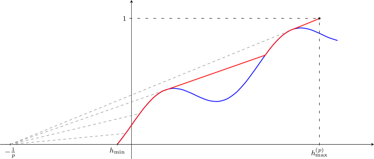
Figure 1: The almost sure $p$-spectrum of a Random Wavelet Series (in red) together with the corresponding wavelet density (in blue).

As in the classical case $p=+\infty$, one can show that if an asymptotic distribution of wavelet coefficients is prescribed, then the $p$-large deviation wavelet formalism is almost surely satisfied, in the sense of prevalence, which constitutes our third main result. Here, the coefficients distribution – given by a so-called admissible profile $\nu$, which defines the space $S^{\nu}$ – is allowed to generate functions that are locally in $L^{p}$, rather than necessarily locally bounded. In Section 5.1, we provide precise definitions of the admissible profiles $\nu$ and of the quantity $p_{\nu}$ used in the next result, to guarantee that $\eta_{f}(p)>0$ for every $f\in S^{\nu}$ and every $p<p_{\nu}$. We also clarify the role of $h_{\min}$ and $h_{\max}^{(p)}$, analogous to those defined in the context of Random Wavelet Series, and show that these quantities can be determined solely from the profile $\nu$.

Theorem 1.7.

For a prevalent set of functions $f$ in $S^{\nu}$, for all $0<p<p_{\nu}$, the support of $\mathscr{D}_{f}^{(p)}$ is $\left[{h_{\min},h_{\max}^{(p)}}\right]$, and $f$ satisfies the $p$-large deviation wavelet formalism.

Our paper is organized as follows. In Section 2, we recall the necessary notations, introduce wavelets, and define the local $\ell^{p}$-norm of wavelet coefficients ($p$-leaders), which allow to characterize the pointwise $p$-regularity. We also review the Hausdorff measure and dimension. Section 3 is devoted to the proof of Theorem 1.4. In Section 4, we focus on the particular case of Random Wavelet Series, including a precise definition of these functions, and we prove Theorem 1.6. In this section, we provide a lower bound for the spectrum, which, combined with the upper bound given by the previous result, shows that the upper bound is optimal. Finally, in Section 5, we recall the notion of prevalence and the spaces $S^{\nu}$, and we prove Theorem 1.7. Some auxiliary results related to Random Wavelet Series are provided in the Appendix A.

In this paper, $\mathbb{N}$ denotes the set $\{1,2,\ldots\}$ of positive integers, whereas $\mathbb{N}_{0}$ denotes the set $\{0,1,2,\ldots\}$ of non-negative integers. Moreover, $\lceil\cdot\rceil$ stands for the ceiling function, defined for every $x\geq 0$ by

$$\lceil x\rceil=\min\{n\in\mathbb{N}_{0}:x\leq n\}.$$

We also adopt the conventions $\inf\emptyset=+\infty$ and $\frac{1}{+\infty}=0$.

2 Notations and definitions

2.1 Wavelets and leaders

We consider a mother wavelet $\psi$ in the Schwartz class. Then the collection

$$\left\{2^{\frac{j}{2}}\psi_{j,k}:j\in\operatorname{\mathbb{N}},k\in\{0,\ldots,2^{j}-1\}\right\}\cup\{\psi_{0,0}=1\},$$

where $\psi_{j,k}$ is the periodized wavelet

$$\psi_{j,k}(x)=\sum_{l\in\operatorname{\mathbb{Z}}}\psi\left(2^{j}(x-l)-k\right),\;x\in\left[{0,1}\right],$$

forms an orthonormal basis of $L^{2}(\left[{0,1}\right])$ (see [38, 20]). We use a $L^{\infty}$-normalisation, in which case any one-periodic function $f$ of $L^{2}$ can be written as

$$f=\sum_{j\in\operatorname{\mathbb{N}}_{0}}\sum_{k=0}^{2^{j}-1}c_{j,k}\psi_{j,k},$$

where the wavelet coefficients of $f$ are defined by

$$c_{j,k}=2^{j}\int_{0}^{1}\psi_{j,k}(x)f(x)\,dx.$$

Note that the wavelet coefficients can be defined even when $f$ does not belong to $L^{2}$.

Dyadic intervals are classically used to index wavelets and wavelet coefficients: if we set $\lambda_{j,k}=\left[{k2^{-j},(k+1)2^{-j}}\right)$, then $\psi_{\lambda_{j,k}}=\psi_{j,k}$ and $c_{\lambda_{j,k}}=c_{j,k}$ for every $k\in\{0,\ldots,2^{j}-1\}$ and every $j\in\operatorname{\mathbb{N}}_{0}$. Therefore, for all $j\in\operatorname{\mathbb{N}}_{0}$, we identify the set of all dyadic intervals at scale $j$, that is, $\{\lambda_{j,k}:k\in\{0,\ldots,2^{j}-1\}\}$, with the set of positions associated with such dyadic intervals, i.e. $\{0,\ldots,2^{j}-1\}$. Those two sets are denoted by $\Lambda_{j}$, and $\Lambda$ is both the set of all dyadic intervals included in $\left[{0,1}\right]$ and the set of pairs $(j,k)$ with $j\in\operatorname{\mathbb{N}}_{0}$ and $k\in\Lambda_{j}$. With these notations, for a fixed wavelet basis, the function $f$ is identified with a sequence $\vec{c}$ of $\operatorname{\mathbb{R}}^{\Lambda}$. Finally, in the context of pointwise properties, it is useful to refer to $\lambda_{j}(x_{0})$ as the only dyadic interval of $\Lambda_{j}$ that contains $x_{0}$.

One can investigate the pointwise regularity of a function $f$ using its wavelet coefficients $\vec{c}$. Similarly to the Hölder case, where the wavelet leaders defined by

$$l_{\lambda}=\sup_{j^{\prime}\geq j}\sup_{\lambda^{\prime}\in\Lambda_{j^{\prime}},\,\lambda^{\prime}\subseteq 3\lambda}\left|{c_{\lambda^{\prime}}}\right|\quad(\lambda\in\Lambda_{j},j\in\operatorname{\mathbb{N}}_{0})$$ (4)

allow to compute the Hölder exponent through a log-log regression [30], one can define quantities, called $p$-leaders, which provide a way to compute the $p$-exponents. In this work, we do not use the classical definition of $p$-leaders as in [34], but rather a version introduced in [42] to facilitate their use. In this case, at each large scale, the local supremum over coefficients in (4) is replaced by the mean of these same coefficients to the power $p$, that is, a weighted $l^{p}$-norm.

Definition 2.1.

Fix $p>0$, a scale $j\in\operatorname{\mathbb{N}}_{0}$ and a dyadic interval $\lambda\in\Lambda_{j}$. The $p$-leader associated to $\lambda$ is

$$l_{\lambda}^{(p)}=\sup_{j^{\prime}\geq j}\left(\sum_{\lambda^{\prime}\in\Lambda_{j^{\prime}},\,\lambda^{\prime}\subseteq 3\lambda}\left|{c_{\lambda^{\prime}}}\right|^{p}2^{-(j^{\prime}-j)}\right)^{\frac{1}{p}}.$$

The main purpose of introducing $p$-leaders is to obtain the following characterization of $p$-regularity. Note that if $p\in(0,1)$, this property is used to define $p$-exponents as in [34].

Proposition 2.2.

[34, 42] Let $f:\left[{0,1}\right]\rightarrow\operatorname{\mathbb{R}}$ and $p\geq 1$ be such that $\eta_{f}(p)>0$. Then for every $x_{0}\in\left[{0,1}\right]$,

$$h^{(p)}_{f}(x_{0})=\liminf_{j\rightarrow+\infty}\frac{\log\left(l_{\lambda_{j}(x_{0})}^{(p)}\right)}{\log\left(2^{-j}\right)}.$$

2.2 Hausdorff measure and dimension

A few fundamental concepts are outlined in this Section; for a more complete treatment, see e.g. [23]. Let $A$ be a subset of $\operatorname{\mathbb{R}}^{d}$ and $\xi:\left[{0,+\infty}\right)\rightarrow\left[{0,+\infty}\right)$ be a function such that $\xi(0)=0$ and $\xi$ is increasing on a neighbourhood of 0. The Hausdorff outer measure at scale $t\in\left({0,+\infty}\right]$ associated with $\xi$ of the set $A$ is defined by

$$\mathcal{H}_{t}^{\xi}(A)=\inf\left\{\sum_{n\in\operatorname{\mathbb{N}}}\xi(\text{diam}(E_{n})):\text{diam}(E_{n})\leq t\text{ and }A\subseteq\bigcup_{n\in\operatorname{\mathbb{N}}}E_{n}\right\}.$$

The Hausdorff measure associated with $\xi$ of the set $A$ is defined by

$$\mathcal{H}^{\xi}(A)=\lim_{t\rightarrow 0^{+}}\mathcal{H}^{\xi}_{t}(A).$$

If $\xi(x)=x^{s}$ with $s\geq 0$, one simply uses the usual notations $\mathcal{H}^{\xi}_{t}(A)=\mathcal{H}^{s}_{t}(A)$ and $\mathcal{H}^{\xi}(A)=\mathcal{H}^{s}(A)$, and these measures are called $s$-dimensional Hausdorff outer measure at scale $t$ and $s$-dimensional Hausdorff measure respectively.

If $A$ is non-empty, it can be proved that the function $s\mapsto\mathcal{H}^{s}(A)$ is non-decreasing and satisfies

$$\mathcal{H}^{s}(A)=+\infty\;\forall s\in\left[{0,h}\right)\quad\text{and}\quad\mathcal{H}^{s}(A)=0\;\forall s\in\left({h,+\infty}\right).$$

This threshold value $h$ is called the Hausdorff dimension of $A$. More precisely,

$$\dim_{\mathcal{H}}A=\left\{\begin{array}[]{ll}\inf\{s\geq 0:\mathcal{H}^{s}(A)=0\}&\text{ if }A\neq\emptyset,\\ -\infty&\text{ if }A=\emptyset.\end{array}\right.$$

Moreover, if there exists a gauge function $\xi$ such that

$$\lim_{r\rightarrow 0^{+}}\frac{\log\xi(r)}{\log r}=h\quad\text{and}\quad\mathcal{H}^{\xi}(A)>0,$$

then

$$\dim_{\mathcal{H}}(A)\geq h.$$

3 Upper bound for the $p$-spectrum

The aim of this section is to prove Theorem 1.4, that is, to provide an upper bound for the $p$-multifractal spectrum of any fixed function $f$ with $p_{0}(f)>0$, for any fixed $p<p_{0}(f)$, recalling that $p_{0}(f)$ is defined in Equation (3). This upper bound is obtained using large deviation estimates on the distribution of the wavelet coefficients $\vec{c}$ of $f$.

3.1 Large deviation estimates of $p$-leaders

We can define $p$-leader versions of the wavelet density and the wavelet profile.

Definition 3.1.

Let $(l^{(p)}_{\lambda})_{\lambda\in\Lambda}$ be the $p$-leaders sequence associated with $\vec{c}$. The $p$-leader density and the $p$-leader profile of $\vec{c}$ are the functions $\rho^{(p)}_{\vec{c}}$ and $\nu^{(p)}_{\vec{c}}$ respectively defined by

$$\rho^{(p)}_{\vec{c}}(\alpha)=\lim_{\varepsilon\rightarrow 0^{+}}\limsup_{j\rightarrow+\infty}\frac{\log_{2}\left(\#\{\lambda\in\Lambda_{j}:2^{-(\alpha+\varepsilon)j}\leq l^{(p)}_{\lambda}\leq 2^{-(\alpha-\varepsilon)j}\}\right)}{j}$$

and

$$\nu^{(p)}_{\vec{c}}(\alpha)=\lim_{\varepsilon\rightarrow 0^{+}}\limsup_{j\rightarrow+\infty}\frac{\log_{2}\left(\#\{\lambda\in\Lambda_{j}:l^{(p)}_{\lambda}\geq 2^{-(\alpha+\varepsilon)j}\}\right)}{j},$$

for every $\alpha\in\operatorname{\mathbb{R}}$.

To avoid the overlap in the sums defining two neighboring $p$-leaders – which is important to preserve independence across dyadic intervals at the same scale when working with independent random wavelet coefficients – we use the following restricted definition and correspondingly adapt the definitions of the density and profile.

Definition 3.2.

Fix $p>0$, a scale $j\in\operatorname{\mathbb{N}}_{0}$, and a dyadic interval $\lambda\in\Lambda_{j}$. The restricted $p$-leader associated with $\lambda$ is defined by

$$e_{\lambda}^{(p)}=\sup_{j^{\prime}\geq j}\left(\sum_{\lambda^{\prime}\in\Lambda_{j^{\prime}},\,\lambda^{\prime}\subseteq\lambda}\left|{c_{\lambda^{\prime}}}\right|^{p}\,2^{-(j^{\prime}-j)}\right)^{\frac{1}{p}}.$$

If we consider these restricted $p$-leaders instead of the classical ones in the definitions of the $p$-leader density and profile, we denote the resulting functions by $\rho_{\vec{c}}^{(p),\ast}$ and $\nu_{\vec{c}}^{(p),\ast}$, in place of $\rho_{\vec{c}}^{(p)}$ and $\nu_{\vec{c}}^{(p)}$.

Let us now compare the density based either on restricted or non-restricted modified $p$-leaders.

Proposition 3.3.

For every $\alpha\in\operatorname{\mathbb{R}}$, one has

$$\rho_{\vec{c}}^{(p)}(\alpha)\leq\rho_{\vec{c}}^{(p),\ast}(\alpha).$$

Proof.

It follows from the fact that for every scale $j\geq 2$ and every $\lambda\in\Lambda_{j}$, if $N(\lambda)$ denotes the set of the three neighbours of $\lambda$ in $\Lambda_{j}$, then

$$l_{\lambda}^{(p)}=\left(\sum_{\mu\in N(\lambda)}\left(e_{\mu}^{(p)}\right)^{p}\right)^{\frac{1}{p}},$$

which entails that for every $j\geq 2$ and every $\varepsilon>0$,

$$\#\{\lambda\in\Lambda_{j}:2^{-(\alpha+\varepsilon)j}\leq l_{\lambda}^{(p)}<2^{-(\alpha-\varepsilon)j}\}\leq 3\cdot\#\{\lambda\in\Lambda_{j}:2^{-(\alpha+2\varepsilon)j}\leq e_{\lambda}^{(p)}<2^{-(\alpha-2\varepsilon)j}\}.$$

∎

Note that, in the case of the $p$-leader profile, the functions $\nu_{\vec{c}}^{(p)}$ and $\nu_{\vec{c}}^{(p),\ast}$ actually coincide on $\operatorname{\mathbb{R}}$. This result can be obtained as in [15], where the classical case $p=+\infty$ is treated.

3.2 Proof of Theorem 1.4

The proof of Theorem 1.4 is decomposed into Proposition 3.5, the previously established Proposition 3.3 and Theorem 3.7, each of which proves one of the following inequalities:

$$\mathscr{D}_{f}^{(p)}(h)\leq\rho_{\vec{c}}^{(p)}(h)\leq\rho_{\vec{c}}^{(p),\ast}(h)\leq\left(h+\frac{1}{p}\right)\sup_{\alpha\in\left({\frac{-1}{p},h}\right]}\frac{\rho_{\vec{c}}(\alpha)}{\alpha+\frac{1}{p}}.$$

The proof of Proposition 3.5 works verbatim as in [15], where the results are established in the case $p=+\infty$. It relies on Lemma 3.4, which itself follows immediately from the characterization of $p$-leaders via $p$-exponents.

Lemma 3.4.

For every $\alpha\geq\frac{-1}{p}$, define

$$F_{j}^{(p)}(\alpha)=\left\{\lambda\in\Lambda_{j}:l_{\lambda}^{(p)}\geq 2^{-\alpha j}\right\}\quad\text{and}\quad E^{(p)}(\alpha)=\limsup_{j\rightarrow+\infty}\bigcup_{\lambda\in F_{j}^{(p)}(\alpha)}\lambda.$$

Then the following holds:

1. If $x_{0}\in E^{(p)}(\alpha)$, then $h^{(p)}_{f}(x_{0})\leq\alpha$.

2. If $h_{f}^{(p)}(x_{0})<\alpha$, then $x_{0}\in E^{(p)}(\alpha)$.

Proposition 3.5.

For every $h\geq\frac{-1}{p}$, we have

$$\mathscr{D}^{(p)}_{f}(h)\leq\rho_{\vec{c}}^{(p)}(h).$$

The central part of this section is therefore to bound the large-deviation estimates of restricted $p$-leaders by our formalism. We will need the following Lemma, which enhances a result of [41] stating that for every $h\geq\frac{-1}{p}$,

$$\mathscr{D}^{(p)}_{f}(h)\leq hp+1.$$

Lemma 3.6.

For every $h\geq\frac{-1}{p}$,

$$\nu_{\vec{c}}^{(p),\ast}(h)\leq hp+1.$$

Proof.

Fix $h\geq\frac{-1}{p}$. Since $\eta_{f}(p)>0$, there exist $\delta>0$ and $J\in\operatorname{\mathbb{N}}$ such that for every $j\geq J$,

$$2^{-j}\sum_{\lambda\in\Lambda_{j}}\left|{c_{\lambda}}\right|^{p}<2^{-\delta j}.$$

It follows that for every $j\geq J$ and every $\varepsilon>0$, one has

$$\#\left\{\lambda\in\Lambda_{j}:e_{\lambda}^{(p)}\geq 2^{-(h+\varepsilon)j}\right\}\leq 2^{(h+\varepsilon)pj}\sum_{\lambda\in\Lambda_{j}}\left(\sup_{j^{\prime}\geq j}\;\sum_{\lambda^{\prime}\subseteq\lambda}\left|{c_{\lambda^{\prime}}}\right|^{p}2^{-(j^{\prime}-j)}\right)<2^{(hp+1+\varepsilon p-\delta)j},$$

hence the conclusion. ∎

Theorem 3.7.

For every $h\geq\frac{-1}{p}$, we have

$$\rho_{\vec{c}}^{(p),\ast}(h)\leq\left(h+\frac{1}{p}\right)\sup_{\alpha\in\left({\frac{-1}{p},h}\right]}\frac{\rho_{\vec{c}}(\alpha)}{\alpha+\frac{1}{p}}.$$

We decompose the proof of Theorem 3.7 into several Lemmas. First, we write

$$h_{\min}=\frac{\eta_{f}(p)}{p}-\frac{1}{p}$$

and treat the case where $h<h_{\min}$.

Lemma 3.8.

For every $h<h_{\min}$, we have

$$\rho_{\vec{c}}^{(p),\ast}(h)=-\infty.$$

Proof.

For every $h<h_{\min}$ and every $\varepsilon>0$ such that $h+\varepsilon<h_{\min}$, since $p\left(h+\varepsilon+\frac{1}{p}\right)<\eta_{f}(p)$, there exists $J\in\operatorname{\mathbb{N}}$ such that for all $j^{\prime}\geq J$,

$$2^{-j^{\prime}}\sum_{\lambda\in\Lambda_{j^{\prime}}}\left|{c_{\lambda^{\prime}}}\right|^{p}<2^{-\left(h+\varepsilon+\frac{1}{p}\right)pj^{\prime}}.$$

Therefore for all $j\geq J$ and all $\lambda\in\Lambda_{j}$,

$$e_{\lambda}^{(p)}\leq 2^{\frac{j}{p}}\sup_{j^{\prime}\geq j}2^{-\left(h+\varepsilon+\frac{1}{p}\right)j^{\prime}}=2^{-(h+\varepsilon)j}.$$

The conclusion follows. ∎

This case being settled, we fix $h\geq h_{\min}$, we assume $\rho^{(p),\ast}_{\vec{c}}(h)>-\infty$ and we consider $\varepsilon>0$ small enough. For every $j\in\mathbb{N}$, we are interested in the set of dyadic intervals $\Lambda_{j}^{(p)}(h,\varepsilon)$ defined by

$$\Lambda_{j}^{(p)}(h,\varepsilon):=\bigl\{\lambda\in\Lambda_{j}\ :\ 2^{-(h+\varepsilon)j}\leq e_{\lambda}^{(p)}\leq 2^{-(h-\varepsilon)j}\bigr\}.$$

For every such interval $\lambda\in\Lambda_{j}^{(p)}(h,\varepsilon)$, in order to derive from the relation

$$2^{-(h+\varepsilon)j}\leq e_{\lambda}^{(p)}\leq 2^{-(h-\varepsilon)j}$$

a control over the wavelet coefficients, we need to determine the "dominating behaviour" of $e_{\lambda}^{(p)}$, i.e. to find a scale $j^{\prime}(\lambda)$ and an order $\alpha(\lambda)$ such that

$$e_{\lambda}^{(p)}\sim\left(\sum_{\lambda^{\prime}\in\Lambda_{j^{\prime}(\lambda)},\,\lambda^{\prime}\subseteq\lambda,\,\left|{c_{\lambda^{\prime}}}\right|\sim 2^{-\alpha(\lambda)j^{\prime}(\lambda)}}\left|{c_{\lambda^{\prime}}}\right|^{p}2^{-(j^{\prime}(\lambda)-j)}\right)^{\frac{1}{p}}.$$

Let us start by showing that such a scale $j^{\prime}(\lambda)$ exists and is bounded by $Cj$ for a positive constant $C$. To that end, we fix any exponent

$$\alpha_{0}\in\left({\frac{-1}{p},h_{\min}}\right).$$

Lemma 3.9.

There exists $J\in\operatorname{\mathbb{N}}$ such that for every $j\geq J$ and every $\lambda\in\Lambda_{j}^{(p)}(h,\varepsilon)$, there exists $j^{\prime}(\lambda)\geq j$ such that

$$2^{-\left(h+\frac{3\varepsilon}{2}\right)pj}\leq\sum_{\lambda^{\prime}\subseteq\lambda}\left|{c_{\lambda^{\prime}}}\right|^{p}2^{-(j^{\prime}(\lambda)-j)}\leq 2^{-(h-\varepsilon)pj}$$ (5)

and

$$j^{\prime}(\lambda)\leq\frac{h+2\varepsilon+\frac{1}{p}}{\alpha_{0}+\frac{1}{p}}j.$$ (6)

Proof.

Using the relation $p\big(\alpha_{0}+\frac{1}{p}\big)<\eta_{f}(p)$, we get the existence of $J\in\operatorname{\mathbb{N}}$ such that

$$2^{-j^{\prime}}\sum_{\lambda^{\prime}\in\Lambda_{j^{\prime}}}\left|{c_{\lambda^{\prime}}}\right|^{p}<2^{-\left(\alpha_{0}+\frac{1}{p}\right)pj^{\prime}}\quad\forall j^{\prime}\geq J.$$ (7)

Moreover, for every $j\geq J$ and every $\lambda\in\Lambda_{j}^{(p)}(h,\varepsilon)$, there exists $j^{\prime}(\lambda)\geq j$ such that

$$2^{-\left(h+\frac{3\varepsilon}{2}\right)j}\leq\left(\sum_{\lambda^{\prime}\subseteq\lambda}\left|{c_{\lambda^{\prime}}}\right|^{p}2^{-(j^{\prime}(\lambda)-j)}\right)^{\frac{1}{p}}\leq 2^{-(h-\varepsilon)j},$$

hence (5) and

$$2^{-j^{\prime}(\lambda)}\sum_{\lambda^{\prime}\subseteq\lambda}\left|{c_{\lambda^{\prime}}}\right|^{p}\geq 2^{-\left(h+2\varepsilon+\frac{1}{p}\right)pj}.$$ (8)

Inequality (7) applied to $j^{\prime}=j^{\prime}(\lambda)$ and Inequality (8) directly imply Condition (6). ∎

Now, we discretize the scales $j^{\prime}(\lambda)$ by considering multiples of the form $A(\lambda)j$, where $A(\lambda)$ belongs to a set $\mathcal{A}$ independent of $j$. To this end, fix $m\in\operatorname{\mathbb{N}}$ sufficiently large, and define

$$\mathcal{A}=\left\{a+\frac{b}{m}:a\in\left\{1,\ldots,\frac{N}{m}\right\},b\in\{0,\ldots,m-1\}\right\},$$

where $N\in\operatorname{\mathbb{N}}$ is chosen such that

$$\frac{N}{m}+1=\left\lceil\frac{h+2\varepsilon+\frac{1}{p}}{\alpha_{0}+\frac{1}{p}}\right\rceil.$$

With this notation, the following result is an immediate consequence of Lemma 3.9.

Corollary 3.10.

To any $j\geq J$ and any $\lambda\in\Lambda_{j}^{(p)}(h,\varepsilon)$, we can associate $A(\lambda)\in\mathcal{A}$ such that Equation (5) is satisfied for

$$j^{\prime}(\lambda)\in\left[{A(\lambda)j,\left(A(\lambda)+\frac{1}{m}\right)j}\right].$$

Secondly, we need to determine which order $\alpha(\lambda)$ dominates the sum at scale $j^{\prime}(\lambda)$, in the sense that

$$\sum_{\lambda^{\prime}\in\Lambda_{j^{\prime}(\lambda)},\,\lambda^{\prime}\subseteq\lambda}\left|{c_{\lambda^{\prime}}}\right|^{p}\sim\sum_{\lambda^{\prime}\in\Lambda_{j^{\prime}(\lambda)},\,\lambda^{\prime}\subseteq\lambda,\,\left|{c_{\lambda^{\prime}}}\right|\sim 2^{-\alpha(\lambda)j^{\prime}(\lambda)}}\left|{c_{\lambda^{\prime}}}\right|^{p}$$

From now on, we assume $\alpha_{0}+\frac{1}{p}>3\varepsilon$. Moreover, we fix $\beta>0$ and $L\in\operatorname{\mathbb{N}}_{0}$ such that $\beta<\alpha_{0}+\frac{1}{p}-3\varepsilon$, $\beta<\frac{1}{m}$ and $\frac{h+2\varepsilon+\frac{1}{p}}{\beta}=L+1$. The following lemma discretizes the different possible orders that can be reached by coefficients $\left|{c_{\lambda^{\prime}}}\right|$ with $\lambda^{\prime}\in\Lambda_{j^{\prime}(\lambda)}$ and $\lambda^{\prime}\subseteq\lambda$.

Lemma 3.11.

For every $j\geq J$, every $\lambda\in\Lambda_{j}^{(p)}(h,\varepsilon)$ and every $\lambda^{\prime}\in\Lambda_{j^{\prime}(\lambda)}$ with $\lambda^{\prime}\subseteq\lambda$, either $\left|{c_{\lambda^{\prime}}}\right|<2^{-(h+2\varepsilon)j}$, or there exists $l(\lambda^{\prime})\in\{1,\ldots,L\}$ such that

$$2^{-\left(l(\lambda^{\prime})\beta+\frac{1}{m}\right)j^{\prime}(\lambda)}2^{\frac{j^{\prime}(\lambda)}{p}}\leq\left|{c_{\lambda^{\prime}}}\right|\leq 2^{-l(\lambda^{\prime})\beta j^{\prime}(\lambda)}2^{\frac{j^{\prime}(\lambda)}{p}}.$$

Moreover, the first case cannot happen simultaneously for all the intervals $\lambda^{\prime}$ considered.

Proof.

Fix $j\geq J$ and $\lambda\in\Lambda_{j}^{(p)}(h,\varepsilon)$. In view of Relation (5), there exists $\lambda^{\prime}\in\Lambda_{j^{\prime}(\lambda)}$ such that $\lambda^{\prime}\subseteq\lambda$ and

$$\left|{c_{\lambda^{\prime}}}\right|\geq 2^{-(h+2\varepsilon)j},$$ (9)

from which follows the last statement, and for each $\lambda^{\prime}\in\Lambda_{j^{\prime}(\lambda)}$ with $\lambda^{\prime}\subseteq\lambda$, we must have

$$\left|{c_{\lambda^{\prime}}}\right|\leq 2^{-(h-\varepsilon)j}2^{\frac{j^{\prime}(\lambda)-j}{p}}.$$

Therefore, to any dyadic interval $\lambda^{\prime}$ of scale $j^{\prime}(\lambda)$ with $\lambda^{\prime}\subseteq\lambda$ and which satisfies (9), if $\alpha(\lambda^{\prime})\geq 0$ is chosen such that

$$\left|{c_{\lambda^{\prime}}}\right|=2^{-\alpha(\lambda^{\prime})j^{\prime}(\lambda)}2^{\frac{j^{\prime}(\lambda)}{p}},$$ (10)

hence

$$\left(h+\frac{1}{p}-\varepsilon\right)\frac{j}{j^{\prime}(\lambda)}\leq\alpha(\lambda^{\prime})\leq(h+2\varepsilon)\frac{j}{j^{\prime}(\lambda)}+\frac{1}{p}.$$

Then, Inequality (6) implies that

$$\alpha_{0}+\frac{1}{p}-3\varepsilon\leq\alpha(\lambda^{\prime})\leq h+\frac{1}{p}+2\varepsilon.$$

But

$$\bigcup_{l=1}^{L}\left[{l\beta,(l+1)\beta}\right]$$

is a covering of $\left[{\alpha_{0}+\frac{1}{p}-3\varepsilon,h+\frac{1}{p}+2\varepsilon}\right]$ formed of intervals of length at most $\frac{1}{m}$. What precedes then shows that for every such $\lambda^{\prime}$, there exists $l(\lambda^{\prime})\in\{1,\ldots,L\}$ such that (10) is satisfied with

$$\alpha(\lambda^{\prime})\in\left[{l(\lambda^{\prime})\beta,l(\lambda^{\prime})\beta+\frac{1}{m}}\right],$$

hence

$$2^{-\left(l(\lambda^{\prime})\beta+\frac{1}{m}\right)j^{\prime}(\lambda)}2^{\frac{j^{\prime}(\lambda)}{p}}\leq\left|{c_{\lambda^{\prime}}}\right|\leq 2^{-l(\lambda^{\prime})\beta j^{\prime}(\lambda)}2^{\frac{j^{\prime}(\lambda)}{p}}$$

as expected. ∎

We now introduce some notations to count the number of coefficients of a given order, according to the possibilities described in the previous lemma.

Definition 3.12.

For every $j\geq J$, every $\lambda\in\Lambda_{j}^{(p)}(h,\varepsilon)$ and every $l\in\{1,\ldots,L\}$, we define $r_{\lambda}(l)\in\{-\infty\}\cup\left[{\frac{j}{j^{\prime}(\lambda)},1}\right]$ such that

$$\#\left\{\lambda^{\prime}\subseteq\lambda:2^{-\left(l\beta+\frac{1}{m}\right)j^{\prime}(\lambda)}2^{\frac{j^{\prime}(\lambda)}{p}}\leq\left|{c_{\lambda^{\prime}}}\right|\leq 2^{-l\beta j^{\prime}(\lambda)}2^{\frac{j^{\prime}(\lambda)}{p}}\right\}=2^{r_{\lambda}(l)j^{\prime}(\lambda)-j}$$

and $r_{\lambda}(0)\in\{-\infty\}\cup\left[{\frac{j}{j^{\prime}(\lambda)},1}\right)$ such that

$$\#\left\{\lambda^{\prime}\subseteq\lambda:\left|{c_{\lambda^{\prime}}}\right|<2^{-(h+2\varepsilon)j}\right\}=2^{r_{\lambda}(0)j^{\prime}(\lambda)-j}.$$

We further define $l_{0}(\lambda)$ as the value in $\{1,\ldots,L\}$ such that $r_{\lambda}(l_{0}(\lambda))\geq 0$ and

$$\sup_{l\in\{1,\ldots,L\}}\left(r_{\lambda}(l)A(\lambda)-l\beta pA(\lambda)\right)=r_{\lambda}(l_{0}(\lambda))A(\lambda)-l_{0}(\lambda)\beta pA(\lambda).$$

Accordingly, the order $\alpha(\lambda)$ that dominates the sum is given by $\alpha(\lambda)=l_{0}(\lambda)\beta-\frac{1}{p}$. More precisely, we have the following lemma, for which we assume that $J$ is large enough so that $(L+1)<2^{\frac{\varepsilon}{2}pJ}$.

Lemma 3.13.

For every $j\geq J$ and every $\lambda\in\Lambda_{j}^{(p)}(h,\varepsilon)$, we have

$$2^{\left(r_{\lambda}(l_{0}(\lambda))A(\lambda)-\left(l_{0}(\lambda)\beta+\frac{1}{m}\right)p\left(A(\lambda)+\frac{1}{m}\right)\right)j}\leq\sum_{\lambda^{\prime}\subseteq\lambda}\left|{c_{\lambda^{\prime}}}\right|^{p}2^{-(j^{\prime}(\lambda)-j)}\leq 2^{\left(r_{\lambda}(l_{0}(\lambda))A(\lambda)-l_{0}(\lambda)\beta pA(\lambda)+\frac{1}{m}+\frac{\varepsilon}{2}p\right)j}.$$

Proof.

The lower bound simply follows from the fact that there exist $2^{r_{\lambda}(l_{0}(\lambda))j^{\prime}(\lambda)-j}$ coefficients $c_{\lambda^{\prime}}$ that satisfy

$$\left|{c_{\lambda^{\prime}}}\right|^{p}2^{-(j^{\prime}(\lambda)-j)}\geq 2^{-\left(l_{0}(\lambda)\beta+\frac{1}{m}\right)pj^{\prime}(\lambda)+j},$$

with $A(\lambda)j\leq j^{\prime}(\lambda)\leq\left(A(\lambda)+\frac{1}{m}\right)j$.

To obtain the upper bound, we partition the set of dyadic intervals $\lambda^{\prime}$ included in $\lambda$ according to the order of $\left|{c_{\lambda^{\prime}}}\right|$, which allows to write

$$\sum_{\lambda^{\prime}\subseteq\lambda}\left|{c_{\lambda^{\prime}}}\right|^{p}2^{-(j^{\prime}(\lambda)-j)} \leq(L+1)2^{\max\left(\sup_{l\in\{1,\ldots,L\}}\left(r_{\lambda}(l)A(\lambda)-l\beta pA(\lambda)+\frac{1}{m}\right),\,(r_{\lambda}(0)-1)A(\lambda)-(h+2\varepsilon)p\right)j}.$$

Then, we notice that the term $(r_{\lambda}(0)-1)A(\lambda)-(h+2\varepsilon)p$ cannot achieve the maximum otherwise

$$\sum_{\lambda^{\prime}\subseteq\lambda}\left|{c_{\lambda^{\prime}}}\right|^{p}2^{-(j^{\prime}(\lambda)-j)}\leq(L+1)2^{(r_{\lambda}(0)-1)A(\lambda)j}2^{-(h+2\varepsilon)pj}<2^{-\left(h+\frac{3\varepsilon}{2}\right)pj}$$

would contradict Equation (5). We use the definition of $l_{0}(\lambda)$ to conclude the proof. ∎

Moreover, we can provide a lower and an upper bound for $r_{\lambda}(l_{0}(\lambda))$, which follow from Lemma 3.13 and Equation (5).

Corollary 3.14.

We have

$$\frac{l_{0}(\lambda)\beta pA(\lambda)-\frac{1}{m}-(h+2\varepsilon)p}{A(\lambda)}\leq r_{\lambda}(l_{0}(\lambda))\leq\frac{\left(l_{0}(\lambda)\beta+\frac{1}{m}\right)\left(A(\lambda)+\frac{1}{m}\right)p-(h-\varepsilon)p}{A(\lambda)}.$$

Up to now, we have established that to every $j\geq J$ and every $\lambda\in\Lambda_{j}^{(p)}(h,\varepsilon)$, we can associate a valur $A(\lambda)\in\mathcal{A}$ and an integer $l_{0}(\lambda)\in\{1,\ldots,L\}$ which indicate the scale and the order of the dominating behaviour in $e_{\lambda}^{(p)}$, in the sense that Corollary 3.10 and Lemma 3.13 are satisfied.

In order to bound $\rho_{\vec{c}}^{(p),\ast}(h)$ by $\left(h+\frac{1}{p}\right)\frac{\rho_{\vec{c}}(\alpha)}{\alpha+\frac{1}{p}}$, where $\rho_{\vec{c}}(\alpha)$ denotes the wavelet density of an exponent $\alpha$ to be determined, we need to control the minimal number of coefficients of a given order $\alpha$ at each scale of a suitably chosen sequence $(j^{\prime}_{n})_{n\in\operatorname{\mathbb{N}}}$.

The first step is to determine a sequence of scales $(j_{n})_{n\in\operatorname{\mathbb{N}}}$, an order $l\in\{1,\ldots,L\}$ and a coefficient $A\in\mathcal{A}$ such that there exist many dyadic intervals $\lambda\in\Lambda_{j_{n}}(h,\varepsilon)$, whose associated $p$-leaders all arise from coefficients of order $l$ at a scale close to $Aj_{n}$. To that end, let us fix $\delta\in\operatorname{\mathbb{R}}$ such that $\delta>0$ and $\rho_{\vec{c}}^{(p),\ast}(h)-3\delta>0$ if $\rho_{\vec{c}}^{(p),\ast}(h)>0$, or $\delta=0$ if $\rho_{\vec{c}}^{(p),\ast}(h)=0$. We also assume that $J$ is large enough to satisfy $NL<2^{\delta J}$ if $\delta>0$.

Lemma 3.15.

There exist a sequence $(j_{n})_{n\in\operatorname{\mathbb{N}}}$, $A\in\mathcal{A}$ and $l\in\{1,\ldots,L\}$ such that for every $n\in\operatorname{\mathbb{N}}$, there exist at least $2^{(\rho_{\vec{c}}^{(p),\ast}(h)-2\delta)j_{n}}$ dyadic intervals $\lambda\in\Lambda_{j_{n}}^{(p)}(h,\varepsilon)$ with $A(\lambda)=A$ and $l_{0}(\lambda)=l$. Moreover, for every such interval $\lambda$, one has

$$\max\left(\frac{l\beta pA-\frac{1}{m}-(h+2\varepsilon)p}{A},\frac{1}{A+\frac{1}{m}}\right)\leq r_{\lambda}(l)\leq\frac{\left(l\beta+\frac{1}{m}\right)\left(A+\frac{1}{m}\right)p-(h-\varepsilon)p}{A}.$$ (11)

Proof.

By definition of $\rho_{\vec{c}}^{(p),\ast}(h)$, there exists an increasing sequence $(j_{n})_{n\in\operatorname{\mathbb{N}}}$ such that $j_{1}\geq J$ and for every $n\in\operatorname{\mathbb{N}}$,

$$2^{(\rho_{\vec{c}}^{(p),\ast}(h)-\delta)j_{n}}\leq\#\Lambda_{j_{n}}^{(p)}(h,\varepsilon)=\sum_{a=1}^{\frac{N}{m}}\sum_{b=0}^{m-1}\sum_{l=1}^{L}\#\Lambda^{(p)}_{j_{n}}\left(h,\varepsilon,a+\frac{b}{m},l\right),$$

where

$$\Lambda_{j_{n}}^{(p)}(h,\varepsilon,A,l)=\left\{\lambda\in\Lambda_{j_{n}}^{(p)}(h,\varepsilon):A(\lambda)=A\text{ and }l_{0}(\lambda)=l\right\}.$$

Therefore, for every $n\in\operatorname{\mathbb{N}}$,

$$2^{(\rho_{\vec{c}}^{(p),\ast}(h)-\delta)j_{n}}\leq NL\sup_{A\in\mathcal{A}}\,\sup_{l\in\{1,\ldots,L\}}\#\Lambda_{j_{n}}^{(p)}(h,\varepsilon,A,l),$$

from which follows the existence of $A_{n}\in\mathcal{A}$, $l_{n}\in\{1,\ldots,L\}$ such that

$$2^{(\rho_{\vec{c}}^{(p),\ast}(h)-2\delta)j_{n}}\leq\#\Lambda_{j_{n}}^{(p)}(h,\varepsilon,A_{n},l_{n}).$$

Using the pigeon hole principle, we may assume that there exist $A\in\mathcal{A}$ and $l\in\{1,\ldots,L\}$ such that for every $n\in\operatorname{\mathbb{N}}$,

$$2^{(\rho_{\vec{c}}^{(p),\ast}(h)-2\delta)j_{n}}\leq\#\Lambda_{j_{n}}^{(p)}(h,\varepsilon,A,l),$$

which is exactly the condition requested in the first statement. Finally, Equation (11) directly follows from Corollary 3.10 and Corollary 3.14. ∎

It remains to address the following difficulty : when considering two $p$-leaders at scale $j_{n}$, as in Lemma 3.15, the scales at which information about their dominating coefficients is available vary between $Aj_{n}$ and $(A+\frac{1}{m})j_{n}$, depending on the specific $p$-leader under consideration. Consequently, we require the following lemma to derive the sequence $(j^{\prime}_{n})_{n\in\operatorname{\mathbb{N}}}$.

Lemma 3.16.

For every $n\in\operatorname{\mathbb{N}}$ large enough, there are at least

$$\max\left(2^{(\rho_{\vec{c}}^{(p),\ast}(h)-3\delta)j_{n}}2^{\left(l\beta pA-\frac{1}{m}-(h+2\varepsilon)p-1\right)j_{n}},1\right)$$

intervals $\lambda^{\prime}$ at a common scale $j_{n}^{\prime}\in\left[{Aj_{n},\left(A+\frac{1}{m}\right)j_{n}}\right]$ such that

$$2^{-\left(l\beta+\frac{1}{m}-\frac{1}{p}\right)j^{\prime}_{n}}\leq\left|{c_{\lambda^{\prime}}}\right|\leq 2^{-\left(l\beta-\frac{1}{m}-\frac{1}{p}\right)j^{\prime}_{n}}.$$

Proof.

With the notations of Lemma 3.15, for every $n\in\operatorname{\mathbb{N}}$ and every $\lambda\in\Lambda_{j_{n}}^{(p)}(h,\varepsilon,A,l)$, there exist $j^{\prime}_{n}(\lambda)\in\left[{Aj_{n},\left(A+\frac{1}{m}\right)j_{n}}\right]$ and $2^{r_{\lambda}(l)j^{\prime}_{n}(\lambda)-j_{n}}$ intervals $\lambda^{\prime}\in\Lambda_{j_{n}^{\prime}(\lambda)}$ satisfying $\lambda^{\prime}\subseteq\lambda$ and

$$2^{-\left(l\beta+\frac{1}{m}\right)j^{\prime}_{n}(\lambda)}2^{\frac{j^{\prime}_{n}(\lambda)}{p}}\leq\left|{c_{\lambda^{\prime}}}\right|\leq 2^{-l\beta j^{\prime}_{n}(\lambda)}2^{\frac{j^{\prime}_{n}(\lambda)}{p}}.$$

But, since $\#\Lambda_{j_{n}}^{(p)}(h,\varepsilon,A,l)\geq 2^{(\rho_{\vec{c}}^{(p),\ast}(h)-2\delta)j_{n}}$, for every $n\in\operatorname{\mathbb{N}}$ large enough so that $\frac{j_{n}}{m}+1\leq 2^{\delta j_{n}}$ if $\delta>0$, one integer value of $\left[{Aj_{n},\left(A+\frac{1}{m}\right)j_{n}}\right]$ must be picked at least $2^{(\rho_{\vec{c}}^{(p),\ast}(h)-3\delta)j_{n}}$ times. The conclusion then follows from Equation (11). ∎

We may now conclude. It remains to assume that the parameters are chosen such that

• $\rho_{\vec{c}}^{(p),\ast}(h)>4p\varepsilon$ if $\rho_{\vec{c}}^{(p),\ast}(h)>0$,

• $3\delta<\frac{1}{m}$,

• $m\geq\frac{1}{p\varepsilon}$, $m\geq\frac{h+\frac{1}{p}+2\varepsilon}{6\varepsilon}$ and

  $$m\geq\frac{\left(2+p\left(h+\frac{1}{p}-2\varepsilon\right)+p\left\lceil\frac{h+\frac{1}{p}+2\varepsilon}{\alpha_{0}+\frac{1}{p}}\right\rceil-\frac{\rho_{\vec{c}}^{(p),\ast}(h)-4p\varepsilon}{h+\frac{1}{p}+2\varepsilon}\right)\left(h+\frac{1}{p}+2\varepsilon\right)}{4\varepsilon(\rho_{\vec{c}}^{(p),\ast}(h)-4p\varepsilon)}.$$

Let us prove a technical lemma.

Lemma 3.17.

If $\rho_{\vec{c}}^{(p),\ast}(h)>0$, then

$$\rho_{\vec{c}}^{(p),\ast}(h)-3\delta+l\beta pA-\frac{1}{m}-(h+2\varepsilon)p-1\geq\frac{\left(A+\frac{1}{m}\right)(\rho_{\vec{c}}^{(p),\ast}(h)-4p\varepsilon)l\beta}{h+\frac{1}{p}+2\varepsilon}$$

for any pair $(A,l)\in\mathcal{A}\times\{1,\ldots,L\}$ that can be obtained from Lemma 3.15.

Proof.

From (11), we know that the pair $(A,l)$ satisfies

$$\frac{1}{A+\frac{1}{m}}\leq\frac{\left(l\beta+\frac{1}{m}\right)\left(A+\frac{1}{m}\right)p-(h-\varepsilon)p}{A}.$$ (12)

We must prove that the function

$$l\mapsto\rho_{\vec{c}}^{(p),\ast}(h)-3\delta+l\beta pA-\frac{1}{m}-(h+2\varepsilon)p-1-\frac{\left(A+\frac{1}{m}\right)(\rho_{\vec{c}}^{(p),\ast}(h)-4p\varepsilon)l\beta}{h+\frac{1}{p}+2\varepsilon}$$

is non-negative. Direct computations show that this function must be non-decreasing, otherwise Lemma 3.6 would be contradicted. As a consequence, it reaches its minimum when $l$ is minimal, i.e. when

$$l=\frac{A}{\beta\left(A+\frac{1}{m}\right)^{2}p}-\frac{1}{m\beta}+\frac{h-\varepsilon}{\beta\left(A+\frac{1}{m}\right)}$$

in view of Conditions (12). Using the inequality

$$\frac{A}{\beta\left(A+\frac{1}{m}\right)^{2}p}-\frac{1}{m\beta}+\frac{h-\varepsilon}{\beta\left(A+\frac{1}{m}\right)}\geq\frac{h+\frac{1}{p}-2\varepsilon}{\beta\left(A+\frac{1}{m}\right)}-\frac{1}{m\beta},$$

the minimum is eventually shown to be non-negative. ∎

We now have all the necessary tools to complete the proof.

Proof of Theorem 3.7.

From Lemmas 3.16 and 3.17, it follows that we have

$$\frac{\rho_{\vec{c}}\left(l\beta-\frac{1}{p}\right)}{l\beta}\geq\left\{\begin{array}[]{ll}0&\text{ if }\rho_{\vec{c}}^{(p),\ast}(h)=0,\\ \frac{\rho_{\vec{c}}^{(p),\ast}(h)-4p\varepsilon}{h+\frac{1}{p}+2\varepsilon}&\text{ if }\rho_{\vec{c}}^{(p),\ast}(h)>0.\end{array}\right.$$

Since $l\beta-\frac{1}{p}\in\left({\frac{-1}{p},h+2\varepsilon}\right]$, we have in both cases

$$\left(h+2\varepsilon+\frac{1}{p}\right)\sup_{\alpha\in\left({\frac{-1}{p},\,h+2\varepsilon}\right]}\frac{\rho_{\vec{c}}(\alpha)}{\alpha+\frac{1}{p}} \geq\left(h+2\varepsilon+\frac{1}{p}\right)\frac{\rho_{\vec{c}}\left(l\beta-\frac{1}{p}\right)}{l\beta}$$

$$\geq\max(\rho_{\vec{c}}^{(p),\ast}(h)-4p\varepsilon,0).$$

The conclusion then follows by letting $\varepsilon$ tend towards 0. ∎

4 Study of the $p$-spectrum of Random Wavelet Series

The aim of this section is to prove that the upper bound obtained in Theorem 1.4 is optimal, that is, to establish Theorem 1.6. To this end, we study Random Wavelet Series, which are defined directly through the distribution of their coefficients. Such series were introduced and studied by Aubry and Jaffard (see [11]), who showed in particular that the statistical distribution of the coefficients accurately reflects the underlying wavelet profile.

We begin by recalling the relevant definitions and known results concerning these Random Wavelet Series. This preliminary step provides the foundation for establishing the optimality of the upper bound.

4.1 Random Wavelet Series

A Random Wavelet Series (RWS) is a process whose wavelet coefficients are drawn at each scale randomly and independently according to a fixed distribution on a fixed probability space $(\Omega,\mathscr{F},\operatorname{\mathbb{P}})$. If

$$f=\sum_{j\in\operatorname{\mathbb{N}}_{0}}\sum_{k=0}^{2^{j}-1}c_{j,k}\psi_{j,k}$$

is a RWS, then $X_{j,k}$ denotes the random variable $\frac{-\log_{2}\left|{c_{j,k}}\right|}{j}$ and $\bm{\rho_{j}}$ is the common distribution of all $2^{j}$ random variables $X_{j,k}$ ($k\in\{0,\ldots,2^{j}-1\}$). In that case,

$$\operatorname{\mathbb{P}}\left(\left|{c_{j,k}}\right|\geq 2^{-\alpha j}\right)=\bm{\rho_{j}}(\left({-\infty,\alpha}\right]).$$

Moreover, for every $\alpha\in\operatorname{\mathbb{R}}$, we set

$$\bm{\rho}(\alpha)=\lim_{\varepsilon\rightarrow 0^{+}}\limsup_{j\rightarrow+\infty}\frac{\log_{2}\left(2^{j}\bm{\rho_{j}}(\left[{\alpha-\varepsilon,\alpha+\varepsilon}\right])\right)}{j}$$

and

$$\bm{\nu}(\alpha)=\lim_{\varepsilon\rightarrow 0^{+}}\limsup_{j\rightarrow+\infty}\frac{\log_{2}\left(2^{j}\bm{\rho_{j}}(\left({-\infty,\alpha+\varepsilon}\right])\right)}{j}.$$

Finally, to any fixed RWS, we associate the set

$$W=\left\{\alpha\in\operatorname{\mathbb{R}}:\forall\varepsilon>0,\,\sum_{j\in\operatorname{\mathbb{N}}_{0}}2^{j}\bm{\rho_{j}}(\left[{\alpha-\varepsilon,\alpha+\varepsilon}\right])=+\infty\right\}$$

and the value

$$h_{\min}=\inf W.$$

In what follows, we will focus on Random Wavelet Series satisfying $\{\alpha\in\operatorname{\mathbb{R}}:\bm{\rho}(\alpha)>0\}\neq\emptyset$, in which case $W\neq\emptyset$. Since $W$ is closed, we know that $h_{\min}$ belongs to $W$.

We now turn to the main purpose of this section, which is to recall how the wavelet density $\rho_{\vec{c}}$ and the wavelet profile $\nu_{\vec{c}}$ of a Random Wavelet Series $f$ are linked with their theoretical counterparts $\bm{\rho}$ and $\bm{\nu}$, as stated in [11]. The case of the density is handled in Proposition 4.1 (for which we provide a modernized proof in Appendix A), and the property concerning the profile follows in Corollary 4.2.

Proposition 4.1.

[11] The following properties are satisfied:

1. $\bm{\rho}(\alpha)>0\Rightarrow\alpha\in W$ and $\bm{\rho}(\alpha)<0\Rightarrow\alpha\notin W$,

2. almost surely, for every $\alpha\in\operatorname{\mathbb{R}}$,

   $$\rho_{\vec{c}}(\alpha)=\left\{\begin{array}[]{ll}\bm{\rho}(\alpha)&\text{ if }\alpha\in W,\\ -\infty&\text{ otherwise}.\end{array}\right.$$

To infer Corollary 4.2, we use on one hand the fact that $h_{\min}$ belongs to $W$ and the monotonicity of the function $\bm{\nu}$, and on the other hand, the fact that $\nu_{\vec{c}}$ and $\bm{\nu}$ are the increasing hulls respectively of $\rho_{\vec{c}}$ and $\bm{\rho}$, that is, Equation (1) and

$$\bm{\nu}(\alpha)=\sup_{\alpha^{\prime}\leq\alpha}\bm{\rho}(\alpha^{\prime})\;\;\forall\alpha\in\operatorname{\mathbb{R}}\text{ such that }\bm{\nu}(\alpha)\geq 0.$$ (13)

Corollary 4.2.

[11] The following properties are satisfied:

1. for every $\alpha\geq h_{\min}$, $\bm{\nu}(\alpha)\geq 0$,

2. almost surely, for every $\alpha\in\operatorname{\mathbb{R}}$,

   $$\nu_{\vec{c}}(\alpha)=\left\{\begin{array}[]{ll}\bm{\nu}(\alpha)&\text{ if }\alpha\geq h_{\min},\\ -\infty&\text{ otherwise.}\end{array}\right.$$

Notice that in order to compute relevantly the multifractal spectrum of a Random Wavelet Series $f$, as done in the seminal paper [11], one needs to ensure that the RWS is uniformly Hölder and therefore to assume that its uniform Hölder exponent is almost surely positive, that is,

$$\liminf_{j\rightarrow+\infty}\frac{-1}{j}\log_{2}\Big(\sup_{\lambda\in\Lambda_{j}}\left|{c_{\lambda}}\right|\Big)>0\quad\text{a.s.}$$

This condition is automatically met as soon as we require the existence of $\gamma>0$ such that $\alpha<\gamma$ implies $\bm{\rho}(\alpha)<0$. Moreover, from this condition follows that, almost surely, there exists $\eta>0$ such that all but finitely many coefficients satisfy $\left|{c_{j,k}}\right|\leq 2^{-\eta j}$.

In this work, since we seek to study the $p$-regularity of $f$, we allow a wider range of exponents $\alpha$ which includes negative values and is determined by the condition $\eta_{f}(p)>0$ almost surely. In this case, there exists $\eta>0$ such that $\left|{c_{j,k}}\right|\leq 2^{-\left(\eta-\frac{1}{p}\right)j}$ with only a possible finite number of exceptions. Notice that this implies $W\subseteq\left({\frac{-1}{p},+\infty}\right)$ and $\bm{\rho}(\alpha)\leq\bm{\nu}(\alpha)\leq 0$ for every $\alpha\leq\frac{-1}{p}$.

4.2 Proof of Theorem 1.6

We consider a Random Wavelet Series

$$f=\sum_{j\in\operatorname{\mathbb{N}}_{0}}\sum_{k=0}^{2^{j}-1}c_{j,k}\psi_{j,k}$$

such that

$$p_{0}\coloneqq\sup\{p>0:\eta_{f}(p)>0\text{ a.s.}\}>0$$

and we consider $p<p_{0}$. For every $\alpha\geq\frac{-1}{p}$ and every $\delta\in\left[{0,1}\right]$, let

$$E(\alpha,\delta)=\limsup_{j\rightarrow+\infty}\bigcup_{k\in F_{j}(\alpha)}B\left(k2^{-j},2^{-\delta j+2\log_{2}j}\right),$$

where

$$F_{j}(\alpha)=\{k\in\{0,\ldots,2^{j}-1\}:\left|{c_{j,k}}\right|\geq 2^{-\alpha j}\}.$$

Write

$$h_{\max}^{(p)}=\inf\left\{h>\frac{-1}{p}:h+\frac{1}{p}=\left(\sup_{\alpha\in\left({\frac{-1}{p},h}\right]}\frac{\bm{\rho}(\alpha)}{\alpha+\frac{1}{p}}\right)^{-1}\right\}.$$

Moreover, let us define $\bm{\lambda}$ by

$$\bm{\lambda}(\alpha)=\limsup_{j\rightarrow+\infty}\frac{1}{j}\log_{2}\left(2^{j}\bm{\rho_{j}}(\left({-\infty,\alpha}\right])\right)$$

for every $\alpha\in\operatorname{\mathbb{R}}$, so that

$$\bm{\nu}(\alpha)=\lim_{\varepsilon\rightarrow 0^{+}}\bm{\lambda}(\alpha+\varepsilon).$$

Since $\bm{\lambda}$ is non-decreasing, the set $\mathcal{D}$ of its discontinuities is at most countable and $\bm{\nu}(\alpha)=\bm{\lambda}(\alpha)$ for every $\alpha\in\operatorname{\mathbb{R}}\setminus\mathcal{D}$. Finally, we assume that $\bm{\nu}(\alpha)>0$ for every $\alpha>h_{\min}$, in which case $\bm{\rho}(\alpha)>0$ for some $\alpha\geq h_{\min}$, as required previously.

In order to determine the almost sure $p$-spectrum of $f$, we need to describe the sets of points sharing the same $p$-exponent and to compute their Hausdorff dimension. As we will see in Lemma 4.5, the sets $E(\alpha,\delta)$ defined above play a key role in this description, which motivates the need to determine their Hausdorff dimension. By classical mass transference principles, this reduces to finding the value of $\delta$ for which $E(\alpha,\delta)$ covers the interval $\left[{0,1}\right]$. This is achieved in Proposition 4.4 (inspired by a result in [11]), which relies on Lemma 4.3 to understand the range of scales in which one can guarantee, under a given dyadic interval, the existence of a coefficient of at least a given order. The following lemma and its proof are adapted from a corresponding result on Lacunary Wavelet Series (see [22]).

Lemma 4.3.

Let $\alpha\geq\frac{-1}{p}$ be such that $\bm{\lambda}(\alpha)>0$. Almost surely, for every $\varepsilon>0$ satisfying $\bm{\lambda}(\alpha)>\varepsilon$, for infinitely many scales $j$ and for all $\lambda\in\Lambda_{j}$, the smallest scale $j_{\alpha}(\lambda)\geq j$ for which there exists $\lambda^{\prime}\in\Lambda_{j_{\alpha}(\lambda)}$ such that $\lambda^{\prime}\subseteq\lambda$ and $\left|{c_{\lambda^{\prime}}}\right|\geq 2^{-\alpha j_{\alpha}(\lambda)}$ satisfies

$$j_{\alpha}(\lambda)\leq\left\lceil\frac{1}{\bm{\lambda}(\alpha)-\varepsilon}(j+\log_{2}j)\right\rceil.$$

Proof.

Fix $M\geq 2$ such that $\bm{\lambda}(\alpha)-\frac{1}{M-1}>0$. We can choose a sequence $(J_{n})_{n\in\operatorname{\mathbb{N}}}$ such that for all $n\in\operatorname{\mathbb{N}}$,

$$2^{J_{n}}\bm{\rho_{J_{n}}}(\left({-\infty,\alpha}\right])>2^{\left(\bm{\lambda}(\alpha)-\frac{1}{M}\right)J_{n}}.$$

For every $n\in\operatorname{\mathbb{N}}$, define

$$j_{n}=\max\left\{j\in\operatorname{\mathbb{N}}:\left\lceil\frac{1}{\bm{\lambda}(\alpha)-\frac{1}{M}}(j+\log_{2}j)\right\rceil\leq J_{n}\right\}.$$

Consider now the event

$$A_{n}=\left\{\exists\lambda\in\Lambda_{j_{n}}\text{ s.t. }\forall j^{\prime}\leq J_{n}\;\forall\lambda^{\prime}\in\Lambda_{j^{\prime}}\text{ with }\lambda^{\prime}\subseteq\lambda,\text{ one has }\left|{c_{\lambda^{\prime}}}\right|<2^{-\alpha j^{\prime}}\right\}$$

for each $n\in\operatorname{\mathbb{N}}$. We have

$$\operatorname{\mathbb{P}}(A_{n}) \leq\sum_{\lambda\in\Lambda_{j_{n}}}\operatorname{\mathbb{P}}\left(\forall\lambda^{\prime}\in\Lambda_{J_{n}}\text{ with }\lambda^{\prime}\subseteq\lambda,\text{ one has }\left|{c_{\lambda^{\prime}}}\right|<2^{-\alpha J_{n}}\right)$$

$$\leq 2^{j_{n}}\left(1-\bm{\rho_{J_{n}}}(\left({-\infty,\alpha}\right])\right)^{2^{J_{n}-j_{n}}}$$

$$\leq 2^{j_{n}}\exp\left(-2^{J_{n}-j_{n}}\bm{\rho_{J_{n}}}(\left({-\infty,\alpha}\right])\right)$$

$$\leq\left(\frac{2}{e}\right)^{j_{n}}.$$

This establishes the convergence of the series $\sum_{n\in\mathbb{N}}\mathbb{P}(A_{n})$, and the Borel-Cantelli lemma then implies that, almost surely, there exists $N\in\mathbb{N}$ such that for all $n\geq N$ and all $\lambda\in\Lambda_{j_{n}}$,

$$j_{\alpha}(\lambda)\leq J_{n}<\left\lceil\frac{1}{\bm{\lambda}(\alpha)-\frac{1}{M-1}}(j_{n}+\log_{2}j_{n})\right\rceil.$$

By intersecting over all $M$ the full-probability events constructed in this way, we obtain that, almost surely, for every sufficiently large $M\in\mathbb{N}$, for infinitely many scales $j$ and for every $\lambda\in\Lambda_{j}$,

$$j_{\alpha}(\lambda)\leq\left\lceil\frac{1}{\bm{\lambda}(\alpha)-\frac{1}{M}}(j+\log_{2}j)\right\rceil,$$

which concludes the proof. ∎

Proposition 4.4.

For every $\alpha\geq\frac{-1}{p}$ such that $\alpha\notin\mathcal{D}$ and $\bm{\nu}(\alpha)>0$, almost surely, for all $\varepsilon>0$ satisfying $\bm{\nu}(\alpha)>\varepsilon$,

$$\left[{0,1}\right]\subseteq E(\alpha,\bm{\nu}(\alpha)-\varepsilon).$$

Proof.

Fix such an $\alpha$, and consider the full probability event given by Lemma 4.3. Clearly, $\bm{\lambda}(\alpha)=\bm{\nu}(\alpha)>0$. Then for every fixed $\varepsilon>0$ satisfying $\bm{\nu}(\alpha)>\varepsilon$, there exists a sequence $(j_{n})_{n\in\operatorname{\mathbb{N}}}$ such that for all $n\in\operatorname{\mathbb{N}}$ and all $\lambda\in\Lambda_{j_{n}}$,

$$j_{\alpha}(\lambda)\leq\left\lceil\frac{1}{\bm{\lambda}(\alpha)-\varepsilon}(j_{n}+\log_{2}j_{n})\right\rceil.$$

In particular, for all $n\in\operatorname{\mathbb{N}}$ and all $x\in\left[{0,1}\right]$, there exist a scale $J_{n}$ satisfying

$$j_{n}\leq J_{n}\leq\left\lceil\frac{1}{\bm{\lambda}(\alpha)-\varepsilon}(j_{n}+\log_{2}j_{n})\right\rceil$$

and a position $K_{n}\in F_{J_{n}}(\alpha)$ such that $\lambda_{J_{n},K_{n}}\subseteq\lambda_{j_{n}}(x)$, in which case

$$|x-K_{n}2^{-J_{n}}|<2^{-j_{n}}\leq 2^{-(\bm{\lambda}(\alpha)-\varepsilon)(J_{n}-1)+\log_{2}j_{n}}\leq 2^{-(\bm{\nu}(\alpha)-\varepsilon)J_{n}+2\log_{2}J_{n}}.$$

This shows that any $x\in\left[{0,1}\right]$ belongs to $E(\alpha,\bm{\nu}(\alpha)-\varepsilon)$, as expected. ∎

As announced, the following Lemma identifies an upper bound for the $p$-exponents of points belonging to $E(\alpha,\delta)$.

Lemma 4.5.

For every $\alpha\geq\frac{-1}{p}$ and every $\delta\in\left({0,1}\right]$,

$$E(\alpha,\delta)\subseteq\left\{x\in\left[{0,1}\right]:h^{(p)}_{f}(x)\leq\frac{\alpha+\frac{1}{p}}{\delta}-\frac{1}{p}\right\}.$$

Proof.

Fix $\alpha\geq\frac{-1}{p}$, $\delta\in\left({0,1}\right]$ and $x\in E(\alpha,\delta)$. By definition, there exists a sequence $(j_{n})_{n\in\operatorname{\mathbb{N}}}$ such that for every $n\in\operatorname{\mathbb{N}}$, there exists $k_{n}\in F_{j_{n}}(\alpha)$ satisfying

$$\left|{x-k_{n}2^{-j_{n}}}\right|<2^{-\delta j_{n}+2\log_{2}j_{n}}.$$

For each $n\in\operatorname{\mathbb{N}}$, we fix $j^{\prime}_{n}=\lfloor\delta j_{n}-2\log_{2}j_{n}\rfloor$, so that $\lambda_{j_{n},k_{n}}\subseteq 3\lambda_{j^{\prime}_{n}}(x)$. It follows that for every $\varepsilon>0$, if $n$ is large enough, then

$$l_{\lambda_{j^{\prime}_{n}}(x)}^{(p)}\geq 2^{-\alpha j_{n}}2^{-\frac{j_{n}-j^{\prime}_{n}}{p}}\geq 2^{-\left(\alpha+\frac{1}{p}\right)\frac{j^{\prime}_{n}}{\delta-\varepsilon}}2^{\frac{j^{\prime}_{n}}{p}}.$$

Since $j^{\prime}_{n}\rightarrow+\infty$ when $n\rightarrow+\infty$, we obtain

$$h_{f}^{(p)}(x)\leq\frac{\alpha+\frac{1}{p}}{\delta-\varepsilon}-\frac{1}{p},$$

and the conclusion follows. ∎

As a straighforward consequence, we get the following inclusion.

Corollary 4.6.

For every $h>\frac{-1}{p}$,

$$\bigcup_{\alpha\in\left({\frac{-1}{p},h}\right]}E\left(\alpha,\frac{\alpha+\frac{1}{p}}{h+\frac{1}{p}}\right)\subseteq\left\{x\in\left[{0,1}\right]:h^{(p)}_{f}(x)\leq h\right\}.$$

The proof of Theorem 1.6 is now based on three main results: Proposition 4.7 deals with the case $h>h_{\max}^{(p)}$ and Proposition 4.8 handles the value $h_{\min}$, while Theorem 4.16 relies on the general mass transference principle stated in Theorem 4.13 to obtain the essential part of the spectrum, to identify when $h$ belongs to the interval $\left[{h_{\min},h_{\max}^{(p)}}\right]$. Notice that the case $h<h_{\min}$ is a straightforward consequence of Theorem 1.4 and Corollary 4.2.

Let us start by showing that $h_{\max}^{(p)}$ is the maximal regularity, a result mentioned in [11] in the case of the Hölder regularity.

Proposition 4.7.

Almost surely, for all $p<p_{0}$ and all $h>h_{\max}^{(p)}$,

$$\mathscr{D}^{(p)}_{f}(h)=-\infty.$$

Proof.

For a fixed $p<p_{0}$, let us show that, almost surely, for every $x\in\left[{0,1}\right]$, $h_{f}^{(p)}(x)\leq h_{\max}^{(p)}$. By definition,

$$h_{\max}^{(p)}+\frac{1}{p}\geq\inf_{\alpha>\frac{-1}{p}}\frac{\alpha+\frac{1}{p}}{\bm{\rho}(\alpha)}.$$

Then for every $\varepsilon>0$, there exists $\alpha_{\varepsilon}>\frac{-1}{p}$ such that

$$\bm{\rho}(\alpha_{\varepsilon})>0\quad\text{and}\quad h_{\max}^{(p)}+\frac{1}{p}+\varepsilon>\frac{\alpha_{\varepsilon}+\frac{1}{p}}{\bm{\rho}(\alpha_{\varepsilon})}.$$

Fix $\varepsilon>0$ and $\delta>0$ such that $\bm{\rho}(\alpha_{\varepsilon})>\delta$. Since $0<\bm{\rho}(\alpha_{\varepsilon})\leq\bm{\lambda}(\alpha_{\varepsilon}+\delta)$, by Lemma 4.3, almost surely, at infinitely many scales $j$,

$$j_{\alpha_{\varepsilon}+\delta}(\lambda)\leq\left\lceil\frac{1}{\bm{\rho}(\alpha_{\varepsilon})-\delta}(j+\log_{2}j)\right\rceil\quad\forall\lambda\in\Lambda_{j}.$$

As a consequence, almost surely, to every $x\in\left[{0,1}\right]$ and to infinitely many scales $j$, it is possible to associate $J_{j}(x)\in\operatorname{\mathbb{N}}$ such that

$$j\leq J_{j}(x)\leq\left\lceil\frac{1}{\bm{\rho}(\alpha_{\varepsilon})-\delta}(j+\log_{2}j)\right\rceil$$

and

$$l_{\lambda_{j}(x)}^{(p)}\geq 2^{-(\alpha_{\varepsilon}+\delta)J_{j}(x)}2^{-\frac{J_{j}(x)-j}{p}}\geq 2^{-\left(\alpha_{\varepsilon}+\delta+\frac{1}{p}\right)\left(\frac{1}{\bm{\rho}(\alpha_{\varepsilon})-\delta}(j+2\log_{2}j)\right)}2^{\frac{j}{p}}.$$

Therefore, almost surely, for every $x\in\left[{0,1}\right]$,

$$h_{f}^{(p)}(x)\leq\frac{\alpha_{\varepsilon}+\frac{1}{p}+\delta}{\bm{\rho}(\alpha_{\varepsilon})-\delta}-\frac{1}{p}\leq h_{\max}^{(p)}+\varepsilon+\frac{\bm{\rho}(\alpha_{\varepsilon})+\alpha_{\varepsilon}+\frac{1}{p}}{\bm{\rho}(\alpha_{\varepsilon})(\bm{\rho}(\alpha_{\varepsilon})-\delta)}\,\delta.$$

Considering sequences $(\delta_{n})_{n\in\operatorname{\mathbb{N}}}$ and $(\varepsilon_{n})_{n\in\operatorname{\mathbb{N}}}$ that converge to 0, we get that, almost surely, for every $x\in\left[{0,1}\right]$,

$$h_{f}^{(p)}(x)\leq h_{\max}^{(p)}.$$

To ensure that the full-probability event does not depend on $p$, let $(p_{n})_{n\in\operatorname{\mathbb{N}}}$ be a dense sequence in $\left({0,p_{0}}\right)$. Then, almost surely, for every $p<p_{0}$ and every $x\in\left[{0,1}\right]$, if $(p_{n}^{\prime})_{n\in\operatorname{\mathbb{N}}}$ is an increasing subsequence of $(p_{n})_{n\in\operatorname{\mathbb{N}}}$ converging to $p$, we have

$$h_{f}^{(p)}(x)\leq h_{f}^{(p_{n}^{\prime})}(x)\leq h_{\max}^{(p_{n}^{\prime})}$$

for every $n\in\operatorname{\mathbb{N}}$, which suffices. ∎

Let us now prove that the minimal regularity $h_{\min}$ is reached. This result is only useful when $\bm{\nu}(h_{\min})=0$, otherwise it follows easily from Remark 4.14.

Proposition 4.8.

Almost surely, for all $p<p_{0}$,

$$\mathscr{D}_{f}^{(p)}(h_{\min})\geq 0.$$

Proof.

Let us show that, almost surely, for all $p<p_{0}$, there exists $x\in\left[{0,1}\right]$ for which $h_{f}^{(p)}(x)=h_{\min}$. For every $j\in\operatorname{\mathbb{N}}$, every $\lambda\in\Lambda_{j}$ and every $\varepsilon>0$, let us write $\Omega(j,\lambda,\varepsilon)$ the event

$$\left\{\exists j^{\prime}>j\;\exists\lambda^{\prime}\in\Lambda_{j^{\prime}}\text{ such that }\lambda^{\prime}\subseteq\lambda\text{ and }\left|{c_{\lambda^{\prime}}}\right|\geq 2^{-\left(h_{\min}+\varepsilon\right)j^{\prime}}\right\}.$$

Since $h_{\min}\in W$, we have

$$\operatorname{\mathbb{P}}(\Omega(j,\lambda,\varepsilon)) =1-\prod_{j^{\prime}>j}\left(1-\bm{\rho_{j^{\prime}}}\left(\left({-\infty,h_{\min}+\varepsilon}\right]\right)\right)^{2^{j^{\prime}-j}}$$

$$\geq 1-\exp\left(-2^{-j}\sum_{j^{\prime}>j}2^{j^{\prime}}\bm{\rho_{j^{\prime}}}(\left[{h_{\min}-\varepsilon,h_{\min}+\varepsilon}\right])\right)$$

$$=1.$$

It follows that the event

$$\bigcap_{j\in\operatorname{\mathbb{N}}}\bigcap_{\lambda\in\Lambda_{j}}\bigcap_{n\in\operatorname{\mathbb{N}}}\Omega\left(j,\lambda,\frac{1}{n}\right)$$

has full probability. But on this event, for every $n\in\operatorname{\mathbb{N}}$, we can construct a decreasing sequence $(\lambda_{m})_{m\in\operatorname{\mathbb{N}}}$ of nested dyadic intervals such that for every $m\in\operatorname{\mathbb{N}}$, $\lambda_{m}\in\Lambda_{j_{m}}$ and $\left|{c_{\lambda_{m}}}\right|\geq 2^{-\left(h_{\min}+\frac{1}{n}\right)j_{m}}$. For each $n\in\operatorname{\mathbb{N}}$, those intervals intersect in a unique point whose $p$-exponents are all equal to $h_{\min}$. ∎

Let us conclude this section with the proof that, almost surely, for every $p<p_{0}$ and every $h\in\left({h_{\min},h_{\max}^{(p)}}\right]$,

$$\mathscr{D}_{f}^{(p)}(h)\geq\left(h+\frac{1}{p}\right)\sup_{\alpha\in\left({\frac{-1}{p},h}\right]}\frac{\bm{\nu}(\alpha)}{\alpha+\frac{1}{p}},$$ (14)

which suffices since $\bm{\nu}\geq\nu_{\vec{c}}$. We first establish in Lemma 4.12 that the proof reduces to finding a suitable gauge function for the set of points whose $p$-exponent is at most $h$. To this end, we need to ensure that Theorem 1.4 also holds for the increasing $p$-spectrum. This is the purpose of Corollary 4.11, which relies on the two following lemmas. The first is an adaptation of Proposition 3.5, and the second can be proved similarly to Equation (1).

Lemma 4.9.

For every $h\geq\frac{-1}{p}$, we have

$$\dim_{\mathcal{H}}\left\{x\in\left[{0,1}\right]:h_{f}^{(p)}(x)\leq h\right\}\leq\nu_{\vec{c}}^{(p)}(h).$$

Lemma 4.10.

For every $\alpha\in\operatorname{\mathbb{R}}$,

$$\nu_{\vec{c}}^{(p)}(\alpha)\leq\sup_{\alpha^{\prime}\leq\alpha}\rho_{\vec{c}}^{(p)}(\alpha^{\prime}).$$

Corollary 4.11.

For every $h\geq\frac{-1}{p}$, we have

$$\dim_{\mathcal{H}}\left\{x\in\left[{0,1}\right]:h_{f}^{(p)}(x)\leq h\right\}\leq\left(h+\frac{1}{p}\right)\sup_{\alpha\in\left({\frac{-1}{p},h}\right]}\frac{\nu_{\vec{c}}(\alpha)}{\alpha+\frac{1}{p}}\leq\left(h+\frac{1}{p}\right)\sup_{\alpha\in\left({\frac{-1}{p},h}\right]}\frac{\bm{\nu}(\alpha)}{\alpha+\frac{1}{p}}.$$

Proof.

This follows by applying in succession Lemma 4.9, Lemma 4.10, Proposition 3.3, Theorem 3.7, and Corollary 4.2. ∎

Lemma 4.12.

Let $p<p_{0}$ and $h\in\left[{h_{\min},h_{\max}^{(p)}}\right]$. If there exists a gauge function $\xi$ satisfying

$$\mathcal{H}^{\xi}\left(\left\{x\in\left[{0,1}\right]:h_{f}^{(p)}(x)\leq h\right\}\right)>0\quad\text{and}\quad\lim_{r\rightarrow 0^{+}}\frac{\log\xi(r)}{\log r}\geq\left(h+\frac{1}{p}\right)\sup_{\alpha\in\left({\frac{-1}{p},h}\right]}\frac{\bm{\nu}(\alpha)}{\alpha+\frac{1}{p}},$$

then Equation (14) is satisfied.

Proof.

We can write

$$\left\{x\in\left[{0,1}\right]:h_{f}^{(p)}(x)=h\right\}=\left\{x\in\left[{0,1}\right]:h_{f}^{(p)}(x)\leq h\right\}\setminus\bigcup_{n\in\operatorname{\mathbb{N}}}\left\{x\in\left[{0,1}\right]:h_{f}^{(p)}(x)\leq h-\frac{1}{n}\right\}$$

and define

$$D_{h}=\left(h+\frac{1}{p}\right)\sup_{\alpha\in\left({\frac{-1}{p},h}\right]}\frac{\bm{\nu}(\alpha)}{\alpha+\frac{1}{p}}.$$

Clearly, for every $n\in\operatorname{\mathbb{N}}$, there exists $\varepsilon_{n}>0$ such that

$$\xi(r)<r^{D_{h-\frac{1}{n}}+\varepsilon_{n}}$$

when $r$ is small enough. It follows that

$$\mathcal{H}^{\xi}\left(\left\{x\in\left[{0,1}\right]:h_{f}^{(p)}(x)\leq h-\frac{1}{n}\right\}\right)=0,$$

because otherwise we would have

$$\dim_{\mathcal{H}}\left\{x\in\left[{0,1}\right]:h_{f}^{(p)}(x)\leq h-\frac{1}{n}\right\}\geq D_{h-\frac{1}{n}}+\varepsilon_{n}>D_{h-\frac{1}{n}}$$

which contradicts Corollary 4.11. Finally, we obtain

$$\mathcal{H}^{\xi}\left(\left\{x\in\left[{0,1}\right]:h_{f}^{(p)}(x)=h\right\}\right)>0,$$

which implies Equation (14). ∎

To construct this gauge function, we will rely on the following result, which corresponds to a simplified version of the general mass transference principle stated in [21, Theorem 2.2]. In our setting, the theorem is applied to the Lebesgue measure on $[0,1]$, which allows for a more straightforward formulation. Note that for every ball $B=B(x,r)$ in $\operatorname{\mathbb{R}}^{d}$ and every $a>0$, $B^{a}$ stands for the ball centered in $x$ and of radius $r^{a}$, i.e. $B^{a}=B(x,r^{a})$.

Theorem 4.13.

Let $(B_{n})_{n\in\operatorname{\mathbb{N}}}$ be a sequence of balls of $\left[{0,1}\right]$ and $(\gamma_{n})_{n\in\operatorname{\mathbb{N}}}\in\left[{1,+\infty}\right)^{\operatorname{\mathbb{N}}}$ a sequence of contracting ratios. Let

$$s=\sup\left\{\frac{1}{\gamma}:\operatorname{\mathcal{L}}\left(\limsup_{k\,:\,\gamma_{k}\leq\gamma}B_{k}\right)=1\right\}.$$

Then there exists a gauge function $\xi:\left[{0,+\infty}\right)\rightarrow\left[{0,+\infty}\right)$ such that

$$\lim_{r\rightarrow 0^{+}}\frac{\log\xi(r)}{\log r}=s\quad\text{and}\quad\mathcal{H}^{\xi}\left(\limsup_{n\rightarrow+\infty}B_{n}^{\gamma_{n}}\right)>0.$$

In order to apply Theorem 4.13 to construct a gauge function as required in Lemma 4.12, one needs to work with a limsup subset of $\left\{x\in\left[{0,1}\right]:h_{f}^{(p)}(x)\leq h\right\}$. However, Corollary 4.6 does not directly provide such a set, so a modification is required. Consider $(\alpha_{n})_{n\in\operatorname{\mathbb{N}}}$ a sequence whose elements belong to $\left({h_{\min},+\infty}\right)\setminus\mathcal{D}$ and which is dense in $\left[{h_{\min},+\infty}\right)$. For every $h\geq h_{\min}$ and every $p<p_{0}$, we set

$$E_{h}^{(p)}=\limsup_{j\rightarrow+\infty}\bigcup_{n\leq j\,:\,\alpha_{n}\leq h}\;\bigcup_{k\in F_{j}(\alpha_{n})}B\left(k2^{-j},2^{\delta_{n}^{(p)}\left(-j+\frac{4}{\bm{\nu}(\alpha_{n})}\log_{2}j\right)}\right),$$ (15)

where

$$\delta_{n}^{(p)}=\frac{\alpha_{n}+\frac{1}{p}}{h+\frac{1}{p}}.$$

Note that the condition $n\leq j$ ensures that, at each scale $j$, a finite number of balls are taken into account in the definition of $E_{h}^{(p)}$, and therefore that it is a limsup set over $j$.

Remark 4.14.

In the case $\bm{\nu}(h_{\min})>0$, we include $h_{\min}$ in the sequence $(\alpha_{n})_{n\in\operatorname{\mathbb{N}}}$. Consequently, Theorem 4.16 also holds at $h=h_{\min}$, so that Proposition 4.8 is encompassed by Theorem 4.16.

Proposition 4.15.

For every $h\geq h_{\min}$ and every $p<p_{0}$,

$$E^{(p)}_{h}\subseteq\left\{x\in\left[{0,1}\right]:h^{(p)}_{f}(x)\leq h\right\}.$$

Proof.

Let $h\geq h_{\min}$, $p<p_{0}$, $x\in E_{h}^{(p)}$ and $\delta>0$ be such that $\eta_{f}(p)>\delta$. By definition of $E_{h}^{(p)}$, there exists a sequence $(j_{m})_{m\in\operatorname{\mathbb{N}}}$ such that for every $m\in\operatorname{\mathbb{N}}$, one can find $\alpha(j_{m})\leq h$ and $k(j_{m})\in\Lambda_{j_{m}}$ satisfying

$$\left|{x-k(j_{m})2^{-j_{m}}}\right|<2^{\delta(j_{m})\left(-j_{m}+\frac{4}{\bm{\nu}(\alpha(j_{m}))}\log_{2}j_{m}\right)}\quad\text{and}\quad\left|{c_{j_{m},k(j_{m})}}\right|\geq 2^{-\alpha(j_{m})j_{m}},$$

with

$$\delta(j_{m})=\frac{\alpha(j_{m})+\frac{1}{p}}{h+\frac{1}{p}}.$$

Moreover, there exists $J\in\operatorname{\mathbb{N}}$ such that for every $j\geq J$ and every $\lambda\in\Lambda_{j}$

$$\left|{c_{\lambda}}\right|<2^{\frac{(1-\delta)j}{p}}.$$

Together, these estimates imply that, for every $m\in\operatorname{\mathbb{N}}$ such that $j_{m}\geq J$,

$$\delta(j_{m})>\frac{\delta}{hp+1}.$$

Hence, the sequence $(\delta(j_{m}))_{n\in\mathbb{N}}$ is bounded from below by a strictly positive constant. Since it is also bounded from above by $1$, we can, up to extraction of a subsequence, assume that it converges to some $l\geq\frac{\delta}{hp+1}>0$. Proceeding as in Lemma 4.5, for each $\varepsilon>0$ and each $m\in\mathbb{N}$, we define

$$j^{\prime}_{m}=\left\lfloor\delta(j_{m})\left(j_{m}-\frac{4}{\bm{\nu}(\alpha(j_{m}))+\varepsilon}\log_{2}j_{m}\right)\right\rfloor,$$

so that $\lambda_{j_{m},k(j_{m})}\subseteq 3\lambda_{j^{\prime}_{m}}(x)$ and, if $m$ is large enough,

$$l_{\lambda_{j^{\prime}_{m}}(x)}^{(p)}\geq 2^{-\alpha(j_{m})j_{n}}2^{-\frac{j_{m}-j^{\prime}_{m}}{p}}\geq 2^{-\left(h+\frac{1}{p}\right)\frac{\delta(j_{m})}{\delta(j_{m})(1-\varepsilon)-\varepsilon}j^{\prime}_{m}}2^{\frac{j^{\prime}_{m}}{p}}.$$

Since $j^{\prime}_{m}\rightarrow+\infty$ when $m\rightarrow+\infty$, we deduce that

$$h_{f}^{(p)}(x)\leq\left(h+\frac{1}{p}\right)\frac{l}{l\,(1-\varepsilon)-\varepsilon}-\frac{1}{p},$$

and the conclusion follows. ∎

We are finally able to prove the last expected result.

Theorem 4.16.

Almost surely, for all $p<p_{0}$ and all $h\in\left({h_{\min},h_{\max}^{(p)}}\right]$,

$$\mathscr{D}^{(p)}_{f}(h)\geq\left(h+\frac{1}{p}\right)\sup_{\alpha\in\left({\frac{-1}{p},h}\right]}\frac{\bm{\nu}(\alpha)}{\alpha+\frac{1}{p}}.$$

Proof.

Using Lemma 4.12 and Proposition 4.15, the proof boils down to showing that, almost surely, for every $p<p_{0}$ and every $h\in\left({h_{\min},h_{\max}^{(p)}}\right]$, there exists a gauge function $\xi$ such that

$$\mathcal{H}^{\xi}\left(E_{h}^{(p)}\right)>0\quad\text{and}\quad\lim_{r\rightarrow 0^{+}}\frac{\log\xi(r)}{\log r}\geq\left(h+\frac{1}{p}\right)\sup_{\alpha\in\left[{h_{\min},h}\right]}\frac{\bm{\nu}(\alpha)}{\alpha+\frac{1}{p}}.$$

Fix $p<p_{0}$ and $h\in\left({h_{\min},h_{\max}^{(p)}}\right]$. These values being fixed, in order not to overcomplicate the notations, we drop the indices. Recall first that $E$, defined from Equation (15), can be viewed as a $\limsup$ set of balls

$$B_{j,n,k}=B\left(k2^{-j},2^{\delta_{n}^{(p)}\left(-j+\frac{4}{\bm{\nu}(\alpha_{n})}\log_{2}j\right)}\right)$$

with $n\leq j$, $\alpha_{n}\leq h$ and $k\in F_{j}(\alpha_{n})$. Now, for every such $n\in\operatorname{\mathbb{N}}$, choose $\varepsilon_{n}>0$ such that $2\varepsilon_{n}<\bm{\nu}(\alpha_{n})$, and define

$$\beta_{n}=\left(h+\frac{1}{p}\right)\frac{\bm{\nu}(\alpha_{n})-\varepsilon_{n}}{\alpha_{n}+\frac{1}{p}}.$$

Notice that

$$0<\left(h_{\min}+\frac{1}{p}\right)\frac{\bm{\nu}(\alpha_{n})-\varepsilon_{n}}{h_{\max}+\frac{1}{p}}\leq\beta_{n}\leq\left(h_{\max}+\frac{1}{p}\right)\frac{\bm{\nu}(\alpha_{n})}{\alpha_{n}+\frac{1}{p}}\leq 1.$$

It follows that $\gamma_{n}=\frac{1}{\beta_{n}}$ is well-defined, larger or equal to 1, and satisfies

$$B_{j,n,k}\supseteq B\left(k2^{-j},2^{-(\bm{\nu}(\alpha_{n})-\varepsilon_{n})j+2\log_{2}j}\right)^{\gamma_{n}}$$

for every $n\in\operatorname{\mathbb{N}}$. For every $(j,n,k)$, we set $\gamma_{j,n,k}=\gamma_{n}$. We only need to construct a full probability event $\Omega^{\ast}$ independent of $h$ and $p$, on which

$$s\coloneqq\sup\left\{\frac{1}{\gamma}:\operatorname{\mathcal{L}}\left(\limsup_{(j,n,k)\,:\,\gamma_{j,n,k}\leq\gamma}B\left(k2^{-j},2^{-(\bm{\nu}(\alpha_{n})-\varepsilon_{n})j+2\log_{2}j}\right)\right)=1\right\}\geq\left(h+\frac{1}{p}\right)\sup_{\alpha\in\left[{h_{\min},h}\right]}\frac{\bm{\nu}(\alpha)}{\alpha+\frac{1}{p}}.$$

Notice that

$$s \geq\sup\left\{\beta_{n}:\operatorname{\mathcal{L}}\left(\limsup_{j\rightarrow+\infty}\bigcup_{k\in F_{j}(\alpha_{n})}B\left(k2^{-j},2^{-(\bm{\nu}(\alpha_{n})-\varepsilon_{n})j+2\log_{2}j}\right)\right)=1\right\}$$

$$=\sup\left\{\beta_{n}:\operatorname{\mathcal{L}}(E(\alpha_{n},\bm{\nu}(\alpha_{n})-\varepsilon_{n}))=1\right\}.$$

In view of Proposition 4.4, there exists a full probability event $\Omega^{\ast}$ independent of $h$ and $p$ such that for every $n\in\operatorname{\mathbb{N}}$ and every $\varepsilon>0$ satisfying $\bm{\nu}(\alpha_{n})>\varepsilon$,

$$\operatorname{\mathcal{L}}(E(\alpha_{n},\bm{\nu}(\alpha_{n})-\varepsilon))=1.$$

It follows that, on $\Omega^{\ast}$,

$$s\geq\left(h+\frac{1}{p}\right)\sup_{n\in\operatorname{\mathbb{N}}}\frac{\bm{\nu}(\alpha_{n})-\varepsilon_{n}}{\alpha_{n}+\frac{1}{p}}=\left(h+\frac{1}{p}\right)\sup_{\alpha\in\left[{h_{\min},h}\right]}\frac{\bm{\nu}(\alpha)}{\alpha+\frac{1}{p}}$$

as expected. ∎

5 Prevalent $p$-spectrum in $S^{\nu}$ spaces

In this section, we prove the generic optimality of the $p$-large deviation wavelet formalism, that is, Theorem 1.7, within the spaces $S^{\nu}$. To this end, we begin by recalling the notion of prevalence, as well as the definition of the spaces $S^{\nu}$.

5.1 Prevalence and $S^{\nu}$ spaces

The notion of prevalence is intended to describe which sets may be considered as large in a measure-theoretic sense. In $\operatorname{\mathbb{R}}^{n}$, a set is typically called small if its Lebesgue measure is null. However, the only locally finite and translation-invariant measure defined on the Borel subsets of an infinite dimensional Banach space is the trivial measure. The notion of prevalence was independently introduced by Christensen ([18]) and Hunt, Sauer and Yorke ([25]) in order to compensate for the lack of such a measure. More precisely, it naturally generalizes the class of null Lebesgue measure sets without the use of a particular measure.

Definition 5.1.

A non-trivial measure $\mu$ defined on the Borel subset of a Polish space $X$ is said to be transverse to a Borel subset $B$ of $X$ if $\mu(B+x)=0$ for every $x\in X$. Furthermore, a Borel subset $B$ of $X$ is said to be shy if there exists a measure that is transverse to $B$. More generally, a subset of $X$ is shy if it can be included in a shy Borel subset of $X$. Moreover, a subset of $X$ is said to be prevalent if its complement is shy.

Let us now recall the definition and some properties of $S^{\nu}$ spaces introduced in [29] (see also [10]). We consider an admissible profile $\nu$, i.e. a function

$$\nu:\operatorname{\mathbb{R}}\rightarrow\{-\infty\}\cup\left[{0,1}\right]$$

which is non-decreasing, right-continuous and satisfies

$$\alpha_{\min}\coloneqq\inf\{\alpha\in\operatorname{\mathbb{R}}:\nu(\alpha)\geq 0\}\in\operatorname{\mathbb{R}}.$$

In this case, $\nu(\alpha)=-\infty$ for every $\alpha<\alpha_{\min}$ and $\nu(\alpha)\geq 0$ for every $\alpha\geq\alpha_{\min}$.

Definition 5.2.

The space $S^{\nu}$ is the set of functions $f$ whose sequence of wavelet coefficients $\vec{c}$ satisfies the following property: for every $\alpha\in\mathbb{R}$, every $\varepsilon>0$, and every $C>0$, there exists $J\in\mathbb{N}$ such that

$$\#\left\{k\in\{0,\ldots,2^{j}-1\}:\left|{c_{j,k}}\right|\geq C2^{-\alpha j}\right\}\leq 2^{(\nu(\alpha)+\varepsilon)j}\,,\quad\forall j\geq J.$$

In other words, $S^{\nu}$ is the space of functions $f$ whose wavelet coefficient sequence $\vec{c}$ satisfies $\nu_{\vec{c}}(\alpha)\leq\nu(\alpha)$ for every $\alpha\in\mathbb{R}$. This space can be shown to be robust (i.e., independent of the choice of a regular wavelet basis used to compute the coefficients), vectorial, metric, complete, and separable [10]. Hence, it is suitable for the study of generic properties. Moreover, it is known from [9] that the set of sequences $\vec{c}\in S^{\nu}$ for which $\nu_{\vec{c}}=\nu$ is prevalent.

5.2 Proof of Theorem 1.7

We fix an admissible profile $\nu$ such that $\nu(\alpha)>0$ for all $\alpha>\alpha_{\min}$. We set

$$p_{\nu}=\inf_{\alpha\in\left[{\alpha_{\min},0}\right)}\frac{\nu(\alpha)-1}{\alpha},$$ (16)

and we assume $\nu(0)<1$ if $\alpha_{\min}\leq 0$. In this case, using the properties

$$\eta_{f}(p)=\sup\left\{s\in\operatorname{\mathbb{R}}:\vec{c}\in b_{p,\infty}^{\frac{s}{p}}\right\}$$

(see [27]) and

$$S^{\nu}\subseteq\bigcap_{\varepsilon>0}b_{p,\infty}^{\frac{\eta(p)}{p}-\varepsilon},\quad\text{with}\quad\eta(p)=\inf_{\alpha\geq\alpha_{\min}}(\alpha p-\nu(\alpha)+1)$$

(see [10]), it can be shown that $\eta_{f}(p)>0$ for all $p<p_{\nu}$ and all $f\in S^{\nu}$, as required.

To establish Theorem 1.7, we rely on the fact that a property $\mathcal{P}$ in a Polish space $E$ is prevalent if one can construct a process $X$ which has almost surely its values in $E$ and such that $X+f$ satisfies $\mathcal{P}$ for all $f\in E$. Indeed, in this case, the distribution of $X$ is transverse to the set of functions in $E$ which do not satisfy $\mathcal{P}$, and its complement is therefore prevalent.

Let us now construct such a process. It follows naturally from Section 4.2 to consider a specific type of Random Wavelet Series.

Definition 5.3.

A RWS is said to be associated to $\nu$ if

• for every $\alpha\in\operatorname{\mathbb{R}}$, one has

  $$\limsup_{j\rightarrow+\infty}\frac{1}{j}\log_{2}\left(2^{j}\bm{\rho_{j}}(\left({-\infty,\alpha}\right])\right)=\nu(\alpha)$$

  i.e. $\nu=\bm{\nu}=\bm{\lambda}$,

• $\nu(\alpha)\geq 0\Rightarrow 2^{j}\bm{\rho_{j}}(\left({-\infty,\alpha}\right])\geq j^{2}$ for every $j\in\operatorname{\mathbb{N}}$.

The existence of a RWS associated to $\nu$ is established in [9], and some of the following properties are mentioned.

Proposition 5.4.

If $f$ is a RWS associated to $\nu$, then, almost surely,

1. one has

   $$h_{\max}^{(p)}=\inf\left\{h>\frac{-1}{p}:h+\frac{1}{p}=\inf_{\alpha\in\left[{\alpha_{\min},h}\right]}\frac{\alpha+\frac{1}{p}}{\nu(\alpha)}\right\},$$

2. $f\in S^{\nu}$, $\alpha_{\min}=h_{\min}$ and $\nu_{\vec{c}}=\nu$,

3. for every $p<p_{\nu}$ and every $h\geq\frac{-1}{p}$,

   $$\mathscr{D}_{f}^{(p)}(h)=\left\{\begin{array}[]{ll}\displaystyle\left(h+\frac{1}{p}\right)\sup_{\alpha\in\left({\frac{-1}{p},h}\right]}\frac{\nu(\alpha)}{\alpha+\frac{1}{p}}&\text{ if }h\leq h_{\max}^{(p)},\\ -\infty&\text{ if }h>h_{\max}^{(p)}.\end{array}\right.$$

Proof.

The first item follows from Equation (13) and the identity $\nu=\bm{\nu}$. Next, Corollary 4.2 ensures that $\nu_{\vec{c}}\leq\bm{\nu}=\nu$ and $\bm{\nu}(h_{\min})\geq 0$, hence $f\in S^{\nu}$ and $h_{\min}\geq\alpha_{\min}$. Moreover, for all $\varepsilon>0$, $\bm{\nu}(\alpha_{\min}-\varepsilon)<0\leq\nu(\alpha_{\min})$, which implies that $\alpha_{\min}$ belongs to $W$, and therefore $\alpha_{\min}\geq h_{\min}$. This is enough to assert $\nu_{\vec{c}}=\nu$, using again Corollary 4.2. Once this property established, the third point follows directly from Theorem 1.6. ∎

Choosing $X$ as a Random Wavelet Series associated to $\nu$ ensures that $X$ almost surely belongs to $S^{\nu}$ and has the required $p$-spectrum. To guarantee that these properties are preserved for $X+f$, we define

$$X=\sum_{j\in\operatorname{\mathbb{N}}_{0}}\sum_{k=0}^{2^{j}-1}C_{j,k}\psi_{j,k},\quad\text{where }C_{j,k}=\varepsilon_{j,k}\left|{C_{j,k}}\right|$$

with $\left|{C_{j,k}}\right|$ chosen such that $X$ is a RWS associated to $\nu$ and $\varepsilon_{j,k}\stackrel{{\scriptstyle\mathrm{i.i.d.}}}{{\sim}}\text{Rademacher}\left(\frac{1}{2}\right)$. Then, $X$ has its values in $S^{\nu}$ and for any fixed

$$f=\sum_{j\in\operatorname{\mathbb{N}}_{0}}\sum_{k=0}^{2^{j}-1}c_{j,k}\psi_{j,k}\in S^{\nu},$$

$$X+f=\sum_{j\in\operatorname{\mathbb{N}}_{0}}\sum_{k=0}^{2^{j}-1}(C_{j,k}+c_{j,k})\psi_{j,k}$$

also has its values in $S^{\nu}$. Though $C_{j,k}+c_{j,k}$ and $C_{j,k^{\prime}}+c_{j,k^{\prime}}$ are independent, there are not necessarily identically distributed, and $X+f$ is not a RWS. It remains to show that the $p$-spectrum of $X+f$ complies with the formalism. To that end, we only need to prove that $X+f$ satisfies a version of Lemma 4.3.

Lemma 5.5.

Let $\alpha\geq\frac{-1}{p}$ be such that $\bm{\lambda}(\alpha)>0$. Almost surely, for every $\varepsilon>0$ satisfying $\bm{\lambda}(\alpha)>\varepsilon$, for infinitely many scales $j$ and for all $\lambda\in\Lambda_{j}$, the smallest scale $J_{\alpha}(\lambda)\geq j$ for which there exists $\lambda^{\prime}\in\Lambda_{J_{\alpha}(\lambda)}$ such that $\lambda^{\prime}\subseteq\lambda$ and $\left|{C_{\lambda^{\prime}}+c_{\lambda^{\prime}}}\right|\geq 2^{-\alpha J_{\alpha}(\lambda)}$ satisfies

$$J_{\alpha}(\lambda)\leq\left\lceil\frac{1}{\bm{\lambda}(\alpha)-\varepsilon}(j+2\log_{2}j)\right\rceil.$$

Proof.

Fix $M\geq 2$ such that $\bm{\lambda}(\alpha)-\frac{1}{M-1}>0$. We can fix sequences $(J_{n})_{n\in\operatorname{\mathbb{N}}}$ and $(j_{n})_{n\in\operatorname{\mathbb{N}}}$ similarly to Lemma 4.3, i.e. such that for all $n\in\operatorname{\mathbb{N}}$,

$$2^{J_{n}}\bm{\rho_{J_{n}}}(\left({-\infty,\alpha}\right])>2^{\left(\bm{\lambda}(\alpha)-\frac{1}{M}\right)J_{n}}$$

and

$$j_{n}=\max\left\{j\in\operatorname{\mathbb{N}}:\left\lceil\frac{1}{\bm{\lambda}(\alpha)-\frac{1}{M}}(j+2\log_{2}j)\right\rceil\leq J_{n}\right\}.$$

For every $n\in\operatorname{\mathbb{N}}$ and every $\lambda\in\Lambda_{j_{n}}$, we consider the sets

$$\Lambda_{n}(\lambda)=\{\lambda^{\prime}\in\Lambda_{J_{n}}:\lambda^{\prime}\subseteq\lambda\},\quad\Lambda_{n}^{+}(\lambda)=\{\lambda^{\prime}\in\Lambda_{n}(\lambda):\left|{C_{\lambda^{\prime}}+c_{\lambda^{\prime}}}\right|\geq\left|{C_{\lambda^{\prime}}}\right|\},$$

the random variable

$$S_{n,\lambda}=\#\Lambda_{n}^{+}(\lambda)=\sum_{\lambda^{\prime}\in\Lambda_{n}(\lambda)}X_{\lambda^{\prime}},\quad\text{where }X_{\lambda^{\prime}}=\left\{\begin{array}[]{ll}1&\text{ if }\lambda^{\prime}\in\Lambda_{n}^{+}(\lambda),\\ 0&\text{otherwise}\end{array}\right.\quad\forall\lambda^{\prime}\in\Lambda_{n}(\lambda),$$

and the event

$$B_{n,\lambda}=\left\{S_{n,\lambda}\geq\frac{2^{J_{n}-j_{n}}}{3}\right\}.$$

We have

$$\mathbb{E}[X_{\lambda^{\prime}}]=\operatorname{\mathbb{P}}\left(\left|{C_{\lambda^{\prime}}+c_{\lambda^{\prime}}}\right|\geq\left|{C_{\lambda^{\prime}}}\right|\right)\geq\operatorname{\mathbb{P}}(\varepsilon_{\lambda^{\prime}}=\text{sgn}(c_{\lambda^{\prime}}))+\mathbb{I}_{\{c_{\lambda^{\prime}}=0\}}\geq\frac{1}{2}$$

for all $\lambda^{\prime}\in\Lambda_{n}(\lambda)$, hence

$$\mathbb{E}[S_{n,\lambda}]\geq\frac{2^{J_{n}-j_{n}}}{2}$$

for all $\lambda\in\Lambda_{j_{n}}$ and all $n\in\operatorname{\mathbb{N}}$. Therefore, using the Hoeffding inequality,

$$\operatorname{\mathbb{P}}(B_{n,\lambda})\geq 1-\operatorname{\mathbb{P}}\left(\mathbb{E}[S_{n,\lambda}]-S_{n,\lambda}\geq\frac{2^{J_{n}-j_{n}}}{6}\right)\geq 1-2e^{-j_{n}}$$

for every $n\in\operatorname{\mathbb{N}}$ such that $2^{J_{n}-j_{n}}\geq 18j_{n}$. Now, for every $n\in\operatorname{\mathbb{N}}$, we define the event

$$A_{n}=\left\{\exists\lambda\in\Lambda_{j_{n}}\text{ s.t. }\forall j^{\prime}\leq J_{n}\,\forall\lambda^{\prime}\in\Lambda_{j^{\prime}}\text{ with }\lambda^{\prime}\subseteq\lambda,\,\left|{C_{\lambda}^{\prime}+c_{\lambda}^{\prime}}\right|<2^{-\alpha j^{\prime}}\right\}.$$

As in Lemma 4.3, it is enough to show that the series $\sum_{n\in\operatorname{\mathbb{N}}}\operatorname{\mathbb{P}}(A_{n})$ converges, which follows from the inequalities

$$\operatorname{\mathbb{P}}(A_{n}) \leq\sum_{\lambda\in\Lambda_{j_{n}}}\operatorname{\mathbb{P}}\left(\forall\lambda^{\prime}\in\Lambda_{J_{n}}\text{ with }\lambda^{\prime}\subseteq\lambda,\,\left|{C_{\lambda}^{\prime}+c_{\lambda}^{\prime}}\right|<2^{-\alpha J_{n}}\right)$$

$$\leq\sum_{\lambda\in\Lambda_{j_{n}}}\operatorname{\mathbb{P}}\left(\forall\lambda^{\prime}\in\Lambda_{n}(\lambda),\,\left|{C_{\lambda}^{\prime}+c_{\lambda}^{\prime}}\right|<2^{-\alpha J_{n}}\,|\,B_{n,\lambda}\right)\operatorname{\mathbb{P}}(B_{n,\lambda})+2^{j_{n}+1}e^{-j_{n}}$$

$$\leq\sum_{\lambda\in\Lambda_{j_{n}}}\operatorname{\mathbb{P}}\left(\forall\lambda^{\prime}\in\Lambda_{n}^{+}(\lambda),\,\left|{C_{\lambda^{\prime}}}\right|<2^{-\alpha J_{n}}\,|\,B_{n,\lambda}\right)\operatorname{\mathbb{P}}(B_{n,\lambda})+2^{j_{n}+1}e^{-j_{n}}$$

$$\leq 2^{j_{n}}\left(1-\bm{\rho_{J_{n}}}(\left({-\infty,\alpha}\right])\right)^{\frac{2^{J_{n}-j_{n}}}{3}}+2^{j_{n}+1}e^{-j_{n}}$$

$$\leq 2^{j_{n}}\exp\left(-\frac{2^{J_{n}-j_{n}}}{3}\bm{\rho_{J_{n}}}(\left({-\infty,\alpha}\right])\right)+2^{j_{n}+1}e^{-j_{n}}$$

$$\leq 2^{j_{n}}e^{\frac{-j_{n}^{2}}{3}}+2^{j_{n}+1}e^{-j_{n}}.$$

∎

Once this lemma is established, the $p$-spectrum follows as in Section 4.2. Note, however, that the lower bound thus provided is equivalently based on $\nu$, $\bm{\nu}$ or $\nu_{\vec{C}}$, but not on the profile $\nu_{\vec{C}+\vec{c}}$ of $X+f$, as would be required to ensure that $X+f$ satisfies the $p$-large deviation wavelet formalism. The prevalence of the set $\{f\in S^{\nu}:\nu_{\vec{c}}=\nu\}$ (stated in Section 5.1) is therefore required to conclude and to get Theorem 1.7, using the fact that the intersection of two prevalent sets is itself prevalent.

Acknowledgements. This work was supported by an FNRS grant awarded to T. Lambert. This project was also partially supported by the Tournesol program, a Partenariat Hubert Curien (PHC). The authors thank E. Daviaud for fruitful discussions that greatly contributed to the development of this study.

Appendix A

The aim of this appendix is to prove Proposition 4.1. To that end, we first recall the following lemma, originally established in [11], which is a direct consequence of the Borel–Cantelli lemma.

Lemma A.1.

Let $a<b$. Almost surely, at infinitely many scales $j$, there exists $\lambda\in\Lambda_{j}$ satisfying

$$2^{-bj}\leq\left|{c_{\lambda}}\right|\leq 2^{-aj}$$

if and only if

$$\sum_{j\in\operatorname{\mathbb{N}}}2^{j}\bm{\rho_{j}}(\left[{a,b}\right])=+\infty.$$

Let us now recall and prove Proposition 4.1.

Proposition A.2.

The following properties are satisfied:

1. $\bm{\rho}(\alpha)>0\Rightarrow\alpha\in W$ and $\bm{\rho}(\alpha)<0\Rightarrow\alpha\notin W$,

2. almost surely, for every $\alpha\in\operatorname{\mathbb{R}}$,

   $$\rho_{\vec{c}}(\alpha)=\left\{\begin{array}[]{ll}\bm{\rho}(\alpha)&\text{ if }\alpha\in W,\\ -\infty&\text{ otherwise}.\end{array}\right.$$

Proof.

Since the first point is clear, we focus on the second item.

First, let us establish that, almost surely, for every $\alpha\notin W$, $\rho_{\vec{c}}(\alpha)=-\infty$. Since $W$ is closed, $\operatorname{\mathbb{R}}\setminus W$ can be written as

$$\operatorname{\mathbb{R}}\setminus W=\bigcup_{n\in\operatorname{\mathbb{N}}}\left({\alpha_{n},\beta_{n}}\right),$$

hence $\alpha\notin W$ if and only if there exist $n\in\operatorname{\mathbb{N}}$ and $m\in\operatorname{\mathbb{N}}$ such that $\frac{1}{m}<\frac{\beta_{n}-\alpha_{n}}{2}$ and

$$\alpha\in\left({\alpha_{n}+\frac{1}{m},\beta_{n}-\frac{1}{m}}\right).$$

Moreover, using the definition of $W$, if $\alpha\notin W$, then there exists $\varepsilon(\alpha)>0$ such that

$$\sum_{j\in\operatorname{\mathbb{N}}}2^{j}\bm{\rho_{j}}(\left[{\alpha-\varepsilon(\alpha),\alpha+\varepsilon(\alpha)}\right])<+\infty.$$

For every $n\in\operatorname{\mathbb{N}}$ and every $m\in\operatorname{\mathbb{N}}$ large enough, one can find $\alpha^{1},\ldots,\alpha^{k}\notin W$, such that the intervals $\left({\alpha^{i}-\varepsilon\left(\alpha^{i}\right),\alpha^{i}+\varepsilon\left(\alpha^{i}\right)}\right)$ cover the compact interval $\left[{\alpha_{n}+\frac{1}{m},\beta_{n}-\frac{1}{m}}\right]$. It follows that for such $n$ and $m$,

$$\sum_{j\in\operatorname{\mathbb{N}}}2^{j}\bm{\rho_{j}}\left(\left[{\alpha_{n}+\frac{1}{m},\beta_{n}-\frac{1}{m}}\right]\right)\leq\sum_{i=1}^{k}\sum_{j\in\operatorname{\mathbb{N}}}2^{j}\bm{\rho_{j}}\left(\left[{\alpha^{i}-\varepsilon(\alpha^{i}),\alpha^{i}+\varepsilon(\alpha^{i})}\right]\right)<+\infty,$$

and Lemma A.1 claims that, almost surely, there exists $J(m,n)\in\operatorname{\mathbb{N}}$ such that for every $j\geq J(m,n)$,

$$\#\left\{\lambda\in\Lambda_{j}:2^{-\left(\beta_{n}-\frac{1}{m}\right)j}\leq\left|{c_{\lambda}}\right|\leq 2^{-\left(\alpha_{n}+\frac{1}{m}\right)j}\right\}=0.$$

The conclusion follows.

Then, to show that, almost surely, for every $\alpha\in W$, $\rho_{\vec{c}}(\alpha)=\bm{\rho}(\alpha)$, we use the first item to divide the proof as follows:

• almost surely, for every $\alpha\in\operatorname{\mathbb{R}}$, $\rho_{\vec{c}}(\alpha)\leq\bm{\rho}(\alpha)$,

• almost surely, for every $\alpha\in\operatorname{\mathbb{R}}$ such that $\bm{\rho}(\alpha)>0$, $\rho_{\vec{c}}(\alpha)\geq\bm{\rho}(\alpha)$,

• almost surely, for every $\alpha\in W$, $\rho_{\vec{c}}(\alpha)\geq 0$.

Note in addition that it is enough to consider $\alpha\in\left({0,1}\right)$. Let us start with item (C). Fix $\varepsilon>0$ and consider a sequence $(\alpha_{n})_{n\in\operatorname{\mathbb{N}}}$ of $W$ such that

$$W\subseteq\bigcup_{n\in\operatorname{\mathbb{N}}}\left({\alpha_{n}-\varepsilon,\alpha_{n}+\varepsilon}\right).$$

By definition of $W$, for every $n\in\operatorname{\mathbb{N}}$,

$$\sum_{j\in\operatorname{\mathbb{N}}}2^{j}\bm{\rho_{j}}(\left[{\alpha_{n}-\varepsilon,\alpha_{n}+\varepsilon}\right])=+\infty.$$

Using Lemma A.1, almost surely, for every $\alpha\in W$, there exists $n\in\operatorname{\mathbb{N}}$ for which, at infinitely many scales $j$, there exists $\lambda\in\Lambda_{j}$ satisfying

$$2^{-(\alpha+2\varepsilon)j}\leq 2^{-(\alpha_{n}+\varepsilon)j}\leq\left|{c_{\lambda}}\right|\leq 2^{-(\alpha_{n}-\varepsilon)j}\leq 2^{-(\alpha-2\varepsilon)j},$$

which allows to conclude by considering a sequence $(\varepsilon_{n})_{n\in\operatorname{\mathbb{N}}}$ that decreases to 0. Let us now move to properties (A) and (B). For every $j\in\operatorname{\mathbb{N}}$, let $A_{j}^{(1)}$ and $A_{j}^{(2)}$ be respectively the events

$$\left\{\exists k^{\prime}\in\Lambda_{\lfloor\log_{2}j\rfloor}\text{ s.t. }\#\{\lambda\in\Lambda_{j}:X_{\lambda}\in\lambda_{\lfloor\log_{2}j\rfloor,k^{\prime}}\}>j^{3}+\frac{3}{2}\cdot 2^{j}\bm{\rho_{j}}(\lambda_{\lfloor\log_{2}j\rfloor,k^{\prime}})\right\}$$

and

$$\left\{\exists k^{\prime}\in\Lambda_{\lfloor\log_{2}j\rfloor}\text{ s.t. }\bm{\rho_{j}}(\lambda_{\lfloor\log_{2}j\rfloor,k^{\prime}})\geq\frac{j^{2}}{2^{j}}\text{ and }\#\{\lambda\in\Lambda_{j}:X_{\lambda}\in\lambda_{\lfloor\log_{2}j\rfloor,k^{\prime}}\}<\frac{1}{2}\cdot 2^{j}\bm{\rho_{j}}(\lambda_{\lfloor\log_{2}j\rfloor,k^{\prime}})\right\}.$$

Assume that

$$\operatorname{\mathbb{P}}\left(\limsup_{j\rightarrow+\infty}A_{j}^{(1)}\right)=\operatorname{\mathbb{P}}\left(\limsup_{j\rightarrow+\infty}A_{j}^{(2)}\right)=0$$ (17)

and let us show that this entails items (A) and (B). We know that, almost surely, there exists $J\in\operatorname{\mathbb{N}}$ such that for every $j\geq J$, one has

$$\#\{\lambda\in\Lambda_{j}:X_{\lambda}\in\lambda_{\lfloor\log_{2}j\rfloor,k^{\prime}}\}\leq j^{3}+\frac{3}{2}\cdot 2^{j}\bm{\rho_{j}}(\lambda_{\lfloor\log_{2}j\rfloor,k^{\prime}})\quad\forall k^{\prime}\in\Lambda_{\lfloor\log_{2}j\rfloor},$$

and

$$\#\{\lambda\in\Lambda_{j}:X_{\lambda}\in\lambda_{\lfloor\log_{2}j\rfloor,k^{\prime}}\}\geq\frac{1}{2}\cdot 2^{j}\bm{\rho_{j}}(\lambda_{\lfloor\log_{2}j\rfloor,k^{\prime}})\quad\forall k^{\prime}\in\Lambda_{\lfloor\log_{2}j\rfloor}\text{ with }\bm{\rho_{j}}(\lambda_{\lfloor\log_{2}j\rfloor,k^{\prime}})\geq\frac{j^{2}}{2^{j}}.$$

On this full-probability event, fix $\alpha\in\left({0,1}\right)$, $(\alpha_{m}^{+})_{m\in\operatorname{\mathbb{N}}}$ a non-increasing dyadic sequence of $\left[{0,1}\right]\setminus\{\alpha\}$ which converges to $\alpha$, $(\alpha^{-}_{m})_{m\in\operatorname{\mathbb{N}}}$ a non-decreasing dyadic sequence of $\left[{0,1}\right]\setminus\{\alpha\}$ which converges to $\alpha$ and $m\in\operatorname{\mathbb{N}}$. There exists $J^{\prime}\in\operatorname{\mathbb{N}}$ such that for every $j^{\prime}\geq J^{\prime}$, there exists $\mathcal{K}_{j^{\prime}}\subseteq\Lambda_{j^{\prime}}$ such that

$$\left[{\alpha_{m}^{-},\alpha_{m}^{+}}\right]=\bigcup_{k^{\prime}\in\mathcal{K}_{j^{\prime}}}\lambda_{j^{\prime},k^{\prime}}.$$

Therefore, for every $j\geq\max\left(J,2^{J^{\prime}}\right)$, if $j^{\prime}=\lfloor\log_{2}j\rfloor$, we have

$$\frac{\log_{2}\left(\#\{\lambda\in\Lambda_{j}:2^{-\alpha_{m}^{+}j}\leq\left|{c_{\lambda}}\right|\leq 2^{-\alpha_{m}^{-}j}\}\right)}{j} \leq\frac{\log_{2}\left(\sum_{k^{\prime}\in\mathcal{K}_{j^{\prime}}}\left(j^{3}+\frac{3}{2}\cdot 2^{j}\bm{\rho_{j}}(\lambda_{j^{\prime},k^{\prime}})\right)\right)}{j}$$

$$\leq\frac{\log_{2}\left(j^{4}+\frac{3}{2}\cdot 2^{j}\bm{\rho_{j}}\left(\left[{\alpha_{m}^{-},\alpha_{m}^{+}}\right]\right)\right)}{j},$$

and property (A) follows. If we assume in addition $\bm{\rho}(\alpha)>0$, then we can consider $\delta>0$, $\varepsilon>0$ and a sequence $(j_{n})_{n\in\operatorname{\mathbb{N}}}$ such that for every $n\in\operatorname{\mathbb{N}}$,

$$2^{j_{n}}\bm{\rho_{j_{n}}}(\left[{\alpha_{m}^{-},\alpha_{m}^{+}}\right])\geq 2^{j_{n}}\bm{\rho_{j_{n}}}(\left[{\alpha-\varepsilon,\alpha+\varepsilon}\right])\geq 2^{\delta j_{n}}.$$

Fix $J^{\prime\prime}\in\operatorname{\mathbb{N}}$ such that for every $j\geq J^{\prime\prime}$, $2^{\delta j}\geq j^{3}$. It follows that for every $n\in\operatorname{\mathbb{N}}$ such that $j_{n}\geq\max\left(2^{J^{\prime}},J^{\prime\prime}\right)$,

$$\sum_{k^{\prime}\in\mathcal{K}_{\lfloor\log_{2}j_{n}\rfloor}}\bm{\rho_{j_{n}}}(\lambda_{\lfloor\log_{2}j_{n}\rfloor,k^{\prime}})=\bm{\rho_{j_{n}}}(\left[{\alpha_{m}^{-},\alpha_{m}^{+}}\right])\geq\frac{j_{n}^{3}}{2^{j_{n}}}.$$

Then the subset

$$\mathcal{K}_{\lfloor\log_{2}j_{n}\rfloor}^{+}=\left\{k^{\prime}\in\mathcal{K}_{\lfloor\log_{2}j_{n}\rfloor}:\bm{\rho_{j_{n}}}(\lambda_{\lfloor\log_{2}j_{n}\rfloor,k^{\prime}})\geq\frac{j_{n}^{2}}{2^{j_{n}}}\right\}$$

of $\mathcal{K}_{\lfloor\log_{2}j_{n}\rfloor}$ is non-empty. Therefore, for every $n\in\operatorname{\mathbb{N}}$ such that $j_{n}\geq\max\left(J,2^{J^{\prime}},J^{\prime\prime}\right)$, if $j^{\prime}_{n}=\lfloor\log_{2}j_{n}\rfloor$, we have

$$\frac{1}{j_{n}}\log_{2}\left(\frac{1}{2}2^{j_{n}}\bm{\rho_{j_{n}}}(\left[{\alpha_{m}^{-},\alpha_{m}^{+}}\right])\right) \leq\frac{1}{j_{n}}\log_{2}\left(\sum_{k^{\prime}\in\mathcal{K}^{+}_{j^{\prime}_{n}}}\frac{1}{2}2^{j_{n}}\bm{\rho_{j_{n}}}(\lambda_{j^{\prime}_{n},k^{\prime}})+\frac{1}{2}j_{n}^{3}\right)$$

$$\leq\frac{1}{j_{n}}\log_{2}\left(\sum_{k^{\prime}\in\mathcal{K}^{+}_{j^{\prime}_{n}}}\#\{\lambda\in\Lambda_{j_{n}}:X_{\lambda}\in\lambda_{j^{\prime}_{n},k^{\prime}}\}+\frac{1}{2}j_{n}^{3}\right)$$

$$\leq\frac{1}{j_{n}}\log_{2}\left(\#\{\lambda\in\Lambda_{j_{n}}:2^{-\alpha_{m}^{+}j_{n}}\leq\left|{c_{\lambda}}\right|\leq 2^{-\alpha_{m}^{-}j_{n}}\}+\frac{1}{2}j_{n}^{3}\right)$$

and property (B) follows. It remains to show that Relation (17) is true. Using Borel-Cantelli Lemma, it is enough to establish the convergence of the series $\sum_{j\in\operatorname{\mathbb{N}}}\operatorname{\mathbb{P}}\left(A_{j}^{(1)}\right)$ and $\sum_{j\in\operatorname{\mathbb{N}}}\operatorname{\mathbb{P}}\left(A_{j}^{(2)}\right)$. Note that for every $j\in\operatorname{\mathbb{N}}$, every $j^{\prime}\leq j$ and every $\lambda^{\prime}\in\Lambda_{j^{\prime}}$,

$$\#\{\lambda\in\Lambda_{j}:X_{\lambda}\in\lambda^{\prime}\}\sim\text{Bin}(2^{j},\bm{\rho_{j}}(\lambda^{\prime})),$$

and recall that (see [45]) if $X\sim\text{Bin}(M,p)$ with $p\in\left({0,1}\right)$, then for every $z>0$,

$$\operatorname{\mathbb{P}}(\left|{X-Mp}\right|\geq z)\leq 2\exp\left(-Mp\left[\left(1+\frac{z}{Mp}\right)\ln\left(1+\frac{z}{Mp}\right)-\frac{z}{Mp}\right]\right).$$ (18)

If $A_{j}^{+}$ and $A_{j}^{-}$ denote respectively the events

$$\left\{\exists\lambda^{\prime}\in\Lambda_{\lfloor\log_{2}j\rfloor}\text{ s.t. }\bm{\rho_{j}}(\lambda^{\prime})\geq\frac{j^{2}}{2^{j}}\text{ and }\left|{2^{j}\bm{\rho_{j}}(\lambda^{\prime})-\#\{\lambda\in\Lambda_{j}:X_{\lambda}\in\lambda^{\prime}\}}\right|>\frac{1}{2}\cdot 2^{j}\bm{\rho_{j}}(\lambda^{\prime})\right\}$$

and

$$\left\{\exists\lambda^{\prime}\in\Lambda_{\lfloor\log_{2}j\rfloor}\text{ s.t. }\bm{\rho_{j}}(\lambda^{\prime})\leq\frac{j^{2}}{2^{j}}\text{ and }\left|{2^{j}\bm{\rho_{j}}(\lambda^{\prime})-\#\{\lambda\in\Lambda_{j}:X_{\lambda}\in\lambda^{\prime}\}}\right|>j^{3}\right\}$$

then

$$\operatorname{\mathbb{P}}\left(A_{j}^{(1)}\right)\leq\operatorname{\mathbb{P}}\left(A_{j}^{+}\right)+\operatorname{\mathbb{P}}\left(A_{j}^{-}\right)\quad\text{and}\quad\operatorname{\mathbb{P}}\left(A_{j}^{(2)}\right)\leq\operatorname{\mathbb{P}}\left(A_{j}^{+}\right).$$

For every $j\in\operatorname{\mathbb{N}}$ and every $\lambda^{\prime}\in\Lambda_{\lfloor\log_{2}j\rfloor}$ such that $\bm{\rho_{j}}(\lambda^{\prime})\geq\frac{j^{2}}{2^{j}}$, using the concentration inequality (18) applied to $X=\#\{\lambda\in\Lambda_{j}:X_{\lambda}\in\lambda^{\prime}\}$ and $z=\frac{1}{2}2^{j}\bm{\rho_{j}}(\lambda^{\prime})$, we get

$$\operatorname{\mathbb{P}}\left(\left|{2^{j}\bm{\rho_{j}}(\lambda^{\prime})-\#\{\lambda\in\Lambda_{j}:X_{\lambda}\in\lambda^{\prime}\}}\right|\geq\frac{1}{2}2^{j}\bm{\rho_{j}}(\lambda^{\prime})\right) \leq 2\exp\left(-2^{j}\bm{\rho_{j}}(\lambda^{\prime})\left[\frac{3}{2}\ln\left(\frac{3}{2}\right)-\frac{1}{2}\right]\right)$$

$$\leq 2\exp\left(-\frac{j^{2}}{10}\right)$$

(if $\bm{\rho_{j}}(\lambda^{\prime})=1$, the result is obvious since $\#\{\lambda\in\Lambda_{j}:X_{\lambda}\in\lambda^{\prime}\}=2^{j}$ almost surely). Therefore, for every $j\in\operatorname{\mathbb{N}}$,

$$\operatorname{\mathbb{P}}\left(A_{j}^{+}\right)\leq 2j\exp\left(-\frac{j^{2}}{10}\right).$$

Moreover, for every $j\in\operatorname{\mathbb{N}}$ and every $\lambda^{\prime}\in\Lambda_{\lfloor\log_{2}j\rfloor}$ such that $\bm{\rho_{j}}(\lambda^{\prime})\leq\frac{j^{2}}{2^{j}}$, using Bienaymé-Tchebychev inequality, we get

$$\operatorname{\mathbb{P}}\left(\left|{2^{j}\bm{\rho_{j}}(\lambda^{\prime})-\#\{\lambda\in\Lambda_{j}:X_{\lambda}\in\lambda^{\prime}\}}\right|>j^{3}\right)\leq\frac{2^{j}\bm{\rho_{j}}(\lambda^{\prime})(1-\bm{\rho_{j}}(\lambda^{\prime}))}{j^{6}}\leq\frac{1}{j^{4}}.$$

Therefore, for every $j\in\operatorname{\mathbb{N}}$,

$$\operatorname{\mathbb{P}}\left(A_{j}^{-}\right)\leq\frac{1}{j^{3}}.$$

This is enough to conclude. ∎

References

- [1] P. Abry, S. Jaffard, R. Leonarduzzi, C. Melot, and H. Wendt. Multifractal analysis based on -exponents and lacunarity exponents. In Fractal geometry and stochastics V., pages 279–313. Cham: Springer, 2015.
- [2] P. Abry, S. Jaffard, R. Leonarduzzi, C. Melot, and H. Wendt. New exponents for pointwise singularity classification. In Recent developments in fractals and related fields, Trends Math., pages 1–37. Birkhäuser/Springer, Cham, 2017.
- [3] P. Abry, S. Jaffard, and H. Wendt. A bridge between geometric measure theory and signal processing: Multifractal analysis. In G. Karlheinz, M. Lacey, J. Ortega-Cerdà, and M. Sodin, editors, Operator-Related Function Theory and Time-Frequency Analysis, pages 1–56. Cham: Springer, 2015.
- [4] P. Abry, S. Jaffard, and H. Wendt. Irregularities and scaling in signal and image processing: Multifractal analysis. Benoit Mandelbrot: A Life in Many Dimensions, M. Frame and N. Cohen, Eds., World Scientific Publishing, pages 31–116, 2015.
- [5] P. Abry, H. Wendt, and S. Jaffard. When Vøan Gogh meets mandelbrot: Multifractal classification of painting’s texture. Signal Processing, 92(11):2650–2661, 2012.
- [6] A. Arneodo, B. Audit, N. Decoster, J.-F. Muzy, and C. Vaillant. Climate disruptions, market crashes, and heart attacks. In A. Bunder and H. Schellnhuber, editors, The Science of Disaster, pages 27–102. Springer, 2002.
- [7] A. Arneodo, E. Bacry, and J.F. Muzy. Random cascades on wavelet dyadic trees. Journal of Mathematical Physics, 39(8):4142–4164, 1998.
- [8] A. Arneodo, N. Decoster, and S.G. Roux. Intermittency, log-normal statistics and multifractal cascade process in high-resolution satellite images of cloud structure. Physical Review Letters, 83(6):1255–1258, 1999.
- [9] J.M. Aubry, F. Bastin, and S. Dispa. Prevalence of multifractal functions in spaces. J. Fourier Anal. Appl., 13(2):175–185, 2007.
- [10] J.M. Aubry, F. Bastin, S. Dispa, and S. Jaffard. Topological properties of the sequence spaces . J. Math. Anal. Appl., 321(1):364–387, 2006.
- [11] J.M. Aubry and S. Jaffard. Random wavelet series. Commun. Math. Phys., 227(3):483–514, 2002.
- [12] P. Balança. Fine regularity of Lévy processes and linear (multi)fractional stable motion. Electronic Journal of Probability, 19(101):1–37, 2014.
- [13] J. Barral, N. Fournier, S. Jaffard, and S. Seuret. A pure jump markov process with a random singularity spectrum. Annals of Probability, 38(5):1924–1946, 2010.
- [14] J. Barral and S. Seuret. The singularity spectrum of Lévy processes in multifractal time. Advances in Mathematics, 214(1):437–468, 2007.
- [15] F. Bastin, C. Esser, and S. Jaffard. Large deviation spectra based on wavelet leaders. Rev. Mat. Iberoam., 32(3):859–890, 2016.
- [16] M. Ben Slimane and C. Mélot. Analysis of a fractal boundary: the graph of the Knopp function. Abstr. Appl. Anal., pages Art. ID 587347, 14, 2015.
- [17] A. P. Calderón and A. Zygmund. Local properties of solutions of elliptic partial differential equations. Stud. Math., 20:171–225, 1961.
- [18] J. P. R. Christensen. On sets of Haar measure zero in abelian Polish groups. Isr. J. Math., 13, 1973.
- [19] C. Coiffard, C. Mélot, and T. Willer. A family of functions with two different spectra of singularities. J. Fourier Anal. Appl., 20(5):961–984, 2014.
- [20] I. Daubechies. Ten Lectures on Wavelets. CBMS-NSF Regional Conference Series in Applied Mathematics, 1992.
- [21] E. Daviaud. A dimensional mass transference principle for Borel probability measures and applications. Adv. Math., 474:47, 2025. Id/No 110304.
- [22] C. Esser and B. Vedel. Lacunary wavelet series on Cantor sets. Preprint, arXiv:2207.03733, 2022.
- [23] K. Falconer. The Geometry of Fractal Sets. Cambridge University Press, 1986.
- [24] E. Gerasimova, B. Audit, S.G. Roux, A. Khalil, F. Argoul, O. Naimark, and A. Arneodo. Multifractal analysis of dynamic infrared imaging of breast cancer. European Physical Journal, 104(6):68001, December 2013.
- [25] B. R. Hunt, T. Sauer, and J. A. Yorke. Prevalence: a translation-invariant “almost every” on infinite- dimensional spaces. Bull. Am. Math. Soc., New Ser., 27(2):217–238, 1992.
- [26] S. Jaffard. The spectrum of singularities of Riemann’s function. Revista Matemática Iberoamericana, 12(2):441–460, 1996.
- [27] S. Jaffard. Multifractal formalism for functions. part I: Results valid for all functions. part II: Self-similar functions. SIAM Journal on Mathematical Analysis, 28(4):944–998, 1997.
- [28] S. Jaffard. On lacunary wavelet series. Ann. Appl. Probab., 10(1):313–329, 2000.
- [29] S. Jaffard. Beyond Besov spaces. I: Distributions of wavelet coefficients. J. Fourier Anal. Appl., 10(3):221–246, 2004.
- [30] S. Jaffard. Wavelet techniques in multifractal analysis. In Fractal geometry and applications: A jubilee of Benoît Mandelbrot., pages 91–151. Providence, RI: American Mathematical Society (AMS), 2004.
- [31] S. Jaffard and B. Martin. Multifractal analysis of the Brjuno function. Inventiones Mathematicae, 212(1):109–132, 2017.
- [32] S. Jaffard and C. Mélot. Wavelet analysis of fractal boundaries. I. Local exponents. Comm. Math. Phys., 258(3):513–539, 2005.
- [33] S. Jaffard and C. Melot. Wavelet analysis of fractal boundaries. II: Multifractal analysis. Commun. Math. Phys., 258(3):541–565, 2005.
- [34] S. Jaffard, C. Melot, R. Leonarduzzi, H. Wendt, P. Abry, S. G. Roux, and M. E. Torres. -exponent and -leaders. I: Negative pointwise regularity. Physica A, 448:300–318, 2016.
- [35] D. La Rocca, N. Zilber, P. Abry, V. van Wassenhove, and P. Ciuciu. Self-similarity and multifractality in human brain activity: A wavelet-based analysis of scale-free brain dynamics. Journal of Neuroscience Methods, 309:175–187, Nov 1 2018.
- [36] B. Lashermes, S.G. Roux, and E. Foufoula-Georgiou. Air pressure, temperature and rainfall: Insights from a joint multifractal analysis. In Proceedings of the American Geophysical Union, Fall Meeting, San Francisco, California, USA, 2005.
- [37] D. Lavallée, S. Lovejoy, D. Schertzer, and S.G. Roux. Nonlinear variability of landscape topography: Multifractal analysis and simulation. In Fractals in Geography, pages 171–205. Prentice Hall, 1993.
- [38] P.G. Lemarié and Y. Meyer. Ondelettes et bases hilbertiennes. Rev. Mat. Iberoamericana, 1, 1986.
- [39] J. Lengyel, S.G. Roux, P. Abry, F. Sémécurbe, and S. Jaffard. Local multifractality in urban systems—the case study of housing prices in the greater paris region. Journal of Physics: Complexity, 3:045005, 2022.
- [40] R. Leonarduzzi, H. Wendt, P. Abry, S. Jaffard, and C. Melot. Finite-resolution effects in -leader multifractal analysis. IEEE Trans. Signal Process., 65(13):3359–3368, 2017.
- [41] R. Leonarduzzi, H. Wendt, P. Abry, S. Jaffard, C. Melot, S. G. Roux, and M. E. Torres. -exponent and -leaders. II: Multifractal analysis. relations to detrended fluctuation analysis. Physica A, 448:319–339, 2016.
- [42] L. Loosveldt and S. Nicolay. Generalized spaces of pointwise regularity: toward a general framework for the WLM. Nonlinearity, 34(9):6561–6586, 2021.
- [43] B.B. Mandelbrot. Intermittent turbulence in self-similar cascades: Divergence of high moments and dimension of the carrier. Journal of Fluid Mechanics, 62:331–358, 1974.
- [44] G. Parisi and U. Frisch. On the singularity structure of fully developed turbulence. Turbulence and Predictability in Geophysical Fluid Dynamics, pages 84–87, 1985.
- [45] W. Stute. The oscillation behavior of empirical processes. Ann. Probab., 10:86–107, 1982.
- [46] J. Lévy Véhel. Medical image segmentation with multifractals. In New Approaches in Classification and Data Analysis, Studies in Classification, Data Analysis, and Knowledge Organization, pages 203–210. Springer, 1994.
- [47] H. Wendt, P. Abry, and S. Jaffard. Bootstrap for empirical multifractal analysis. IEEE Signal Processing Magazine, 24(4):38–48, 2007.