Oscillations of the solar photospheric magnetic field
caused by the high-latitude inertial mode
Periodic oscillations at 338 nHz in the Earth frame are observed at high latitudes in direct Doppler velocity measurements. These oscillations correspond to the high-latitude global mode of inertial oscillation. In this study, we investigate the signature of this mode in the photospheric magnetic field using long-term series of line-of-sight magnetograms from the Helioseismic and Magnetic Imager (HMI) and the Global Oscillation Network Group (GONG). Through direct observations and spectral analysis, we detect periodic magnetic field oscillations at high latitudes (–) with a frequency of 338 nHz in the Earth frame, matching the known frequency of the high-latitude inertial mode. The observed line-of-sight magnetic field oscillations are predominantly symmetric across the equator. We find a peak magnetic oscillation amplitude of up to gauss and a distinct spatial pattern, both consistent with simplified model calculations in which the radial component of the magnetic field is advected by the mode’s horizontal flow field.
Key Words.:
Sun: magnetic fields – Sun: oscillations – Sun: interior – Sun: photosphere – Sun: activity – Sun: rotation1 Introduction
The Sun supports periodic and quasi-periodic oscillations over a wide range of spatial and temporal scales. In addition to the well-known five-minute acoustic modes of oscillation, it also exhibits quasi-toroidal modes in the inertial frequency range, with frequencies comparable to the solar rotation frequency. Solar equatorial Rossby modes were first detected by Löptien et al. (2018) and later confirmed by Liang et al. (2019) and Hanasoge & Mandal (2019). A rich spectrum of additional inertial modes, all retrograde in the Carrington frame, were identified in frequency-latitude space by Gizon et al. (2021). Among these modes, the mode with the largest amplitude is an high-latitude mode with north-south symmetric radial vorticity. The amplitude of this mode can be as high as m/s at times. It is believed to be baroclinically-unstable (Bekki et al., 2022) and saturates via a nonlinear interaction with the Sun’s latitudinal differential rotation (Bekki et al., 2024). The velocity features associated with this mode had been noticed at high latitudes by various authors, however it was not then identified as a global mode of oscillation (Ulrich, 1993, 2001; Hathaway et al., 2013; Bogart et al., 2015). For a recent review of solar inertial modes, we refer to Gizon et al. (2024).
The high-latitude modes were initially identified in long time series of near-surface flows in the longitudinal () and colatitudinal () directions. In particular, modes with and both north-south symmetries were observed within 3 nHz of each other (Gizon et al., 2021). The mode with the significantly larger amplitude is anti-symmetric in (symmetric in radial vorticity) and has a frequency nHz in the Carrington frame, with a linewidth of nHz and a mean amplitude of m/s over the period 2010–2020 (Gizon et al., 2021). The latitude at maximum amplitude was determined to be close to . In a recent paper, Liang & Gizon (2025, hereafter LG25) measured the mode amplitude in direct Doppler data and found that the mode has remained visible above latitude throughout the last five solar cycles since 1967. LG25 reported that the mode amplitude exhibits a negative correlation of with the sunspot number and a strong negative correlation of with the differential rotation rate near the mode’s critical latitude (the latitude at which its phase speed equals the rotational velocity).
In the present paper, we show that the high-latitude inertial mode is detectable in the line-of-sight (LOS) photospheric magnetic field, and we study the temporal evolution of its amplitude over a period of 17 years ( to ). In Sect. 2 we describe the datasets used. We detect and charactewrize the magnetic field oscillations in Sect. 3 and compare them to the velocity oscillations in Sect. 4. The results are discussed in Sect. 5.
2 Observational datasets
To investigate oscillations in the photospheric LOS magnetic field () in the inertial frequency range, we analyze two long-term datasets. We use 720-s cadence LOS magnetograms taken by the Helioseismic and Magnetic Imager (HMI; Schou et al., 2012) onboard the Solar Dynamics Observatory (SDO; Pesnell et al., 2012) over a time period of more than 14 years (2010–2024), as well as daily merged magnetograms from the Global Oscillation Network Group (GONG; Harvey et al., 1996) spanning 17 years (2007–2024). We compile the datasets at a one-day cadence by computing daily averages when multiple images are available each day. The duty cycle of the daily averages is nearly for both HMI and GONG datasets. The original magnetograms have pixels for HMI and pixels for GONG. Unlike LG25, we did not use the Mount Wilson data because its signal-to-noise ratio is significantly lower.
The data reduction procedure, which is the same for both datasets, is as follows. Daily magnetograms are binned down to pixels and remapped onto a uniform grid in Stonyhurst longitude () and latitude () with a grid spacing of in both coordinates. We then compute the latitudinally symmetric component of the magnetic field as
| (1) |
We also computed the anti-symmetric component of , but found no significant signal in the neighborhood of the mode frequency.
To further increase the signal-to-noise ratio, we consider averages of in longitude at every time step:
| (2) |
where is the number of longitude bins in the sum. To detect a perturbation in the magnetic field that may be associated with the high-latitude mode, we investigate the evolution of the magnetic field in the latitude range where the mode’s amplitude is most prominent (around or beyond , see Gizon et al., 2021). We define latitudinal average of over the latitude band :
| (3) |
where the is the number of latitude bins in the sum.
To compare with the mode characteristics derived from the reduced LOS Doppler velocity (), we also compute the following quantities from the HMI and GONG Dopplergrams (see LG25 for details):
| (4) | ||||
| (5) | ||||
| (6) |
The zonal velocity, , serves as a proxy for the longitudinal component of surface velocity (Ulrich, 2001).
3 Detection of the mode in magnetograms
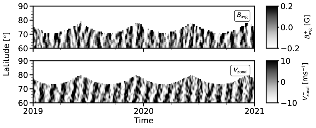
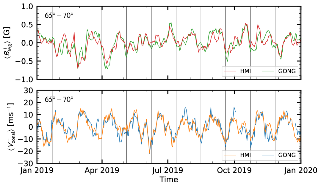
Figure 1 shows supersynoptic maps of and at high latitudes. An oscillating pattern in both observables is evident in both quantities with a temporal cadence of approximately 34 days. The oscillation is also clearly visible in the spatially averaged data and in Fig. 2. We find an amplitude of up to G for , associated with the already known amplitude of 10–20 m/s for in the latitude range –. Since the magnetic field evolution appears to be tightly related to that of the mode observed in the Doppler data (LG25), this strongly suggests the presence of the mode in the magnetograms; however, this still needs to be verified through spectral analysis.
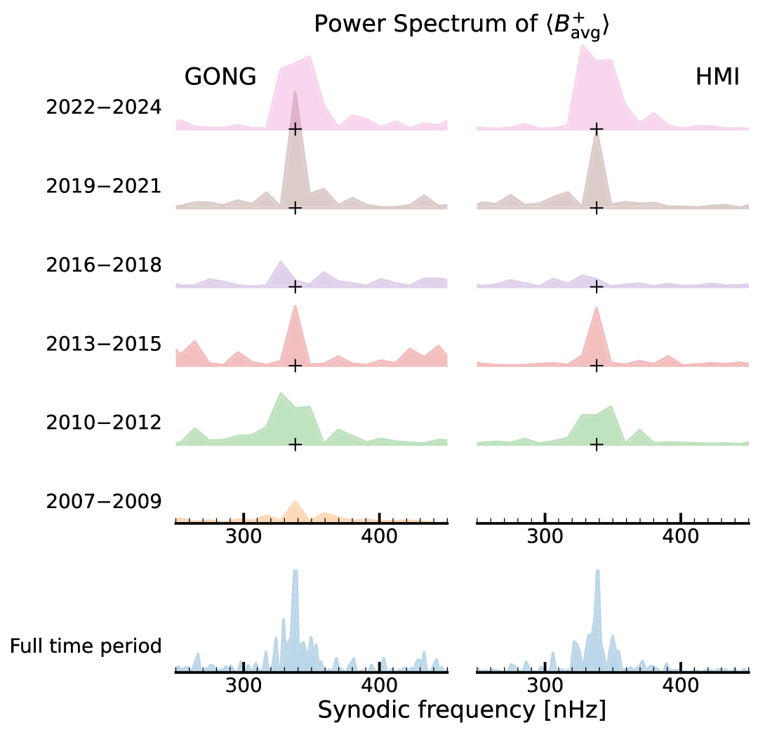
3.1 Power spectra
We examine in the frequency domain by performing a Fourier transform over the full time period available in each dataset. The power spectra were rescaled to account for the missing data in the time series. In the bottom row of Fig. 3, we show the power spectra of for the full HMI and GONG datasets. In both spectra, we find strong excess power around 338 nHz, with a full width at half maximum of approximately – nHz (corresponding to an e-folding lifetime of – months). We recall that the frequency of the mode was reported by (Gizon et al., 2021) to be nHz in the Carrington frame. In the Earth frame the mode frequency is
| (7) |
where nHz is the Carrington rotation rate and nHz is the Earth’s mean orbital frequency around the Sun.
Figure 3 further shows changes of the power spectra of in three-year intervals for GONG and HMI data. It is evident that the signal is not uniformly strong over the entire time period, neither persistently present (i.e., significant); instead, it shows a pattern of rising and waning over cycle 24. The strongest and clearest signal is observed during the solar minimum interval of 2019–2021 with a peak amplitude of G2 nHz-1, while no significant signal is observed during 2016–2018. We also find a clear signal during 2010–2015 with a peak amplitude of G2 nHz-1. GONG and HMI results show very good agreement.
3.2 Latitudinal variation of phase
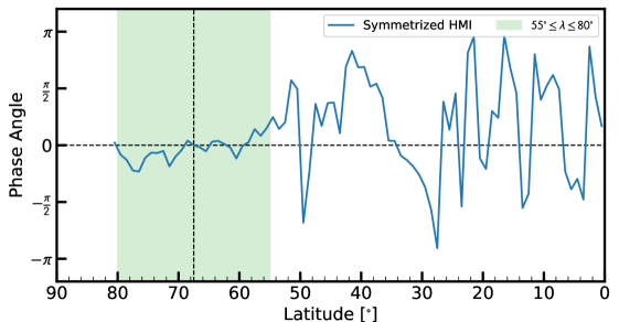
We calculated the average phase of as a function of latitude using a temporal Fourier transform. Phase shifts relative to latitude were extracted within a narrow band centered at 338 nHz (10 nHz) and then averaged. The resulting phase, wrapped to the interval [, ], varies smoothly between and latitude (see Fig. 6 in the Appendix). The smooth variation suggests that the excess power at higher latitudes reflects a genuine mode signal rather than stochastic fluctuations. The phase becomes irregular at lower latitudes, where the mode power is not significant.
4 Comparison of and
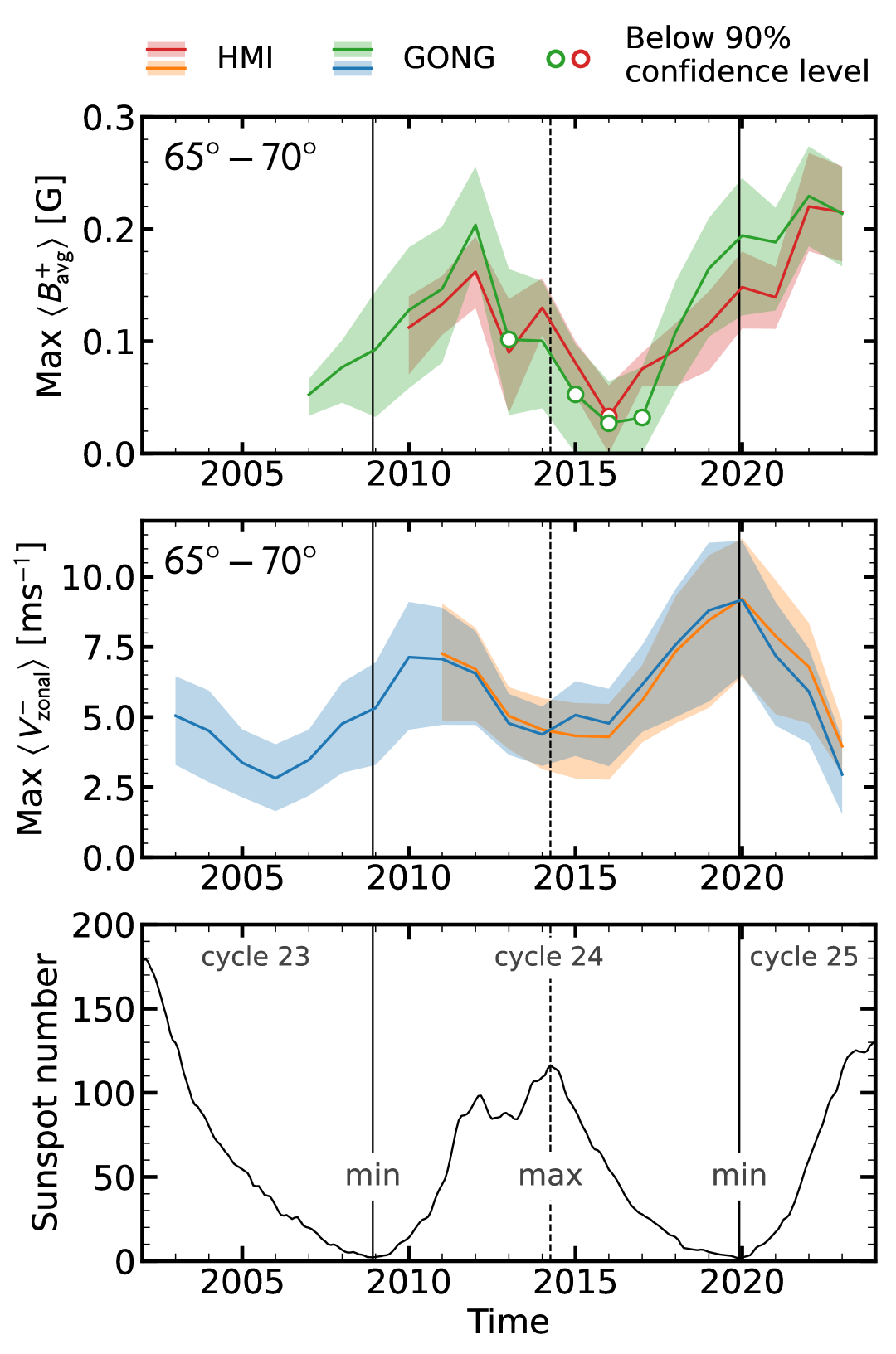
We now compare the excess power around 338 nHz in the and spectra. Following the procedure described by LG25 (their section 5.2), we estimate the total power around the mode frequency by fitting a Lorentzian function. Figure 4 shows the temporal variations of the mode amplitude measured from overlapping 3-yr time series, with central times spaced one year apart, starting in 2007 for and in 2003 for .
We find very good agreement between the GONG and HMI results for each respective quantity. The mode amplitudes seen in and are positively correlated, but there is a time lag between the magnetic field and velocity perturbations. The maximum amplitude in is about G in 2012 and again around 2020–2023. Both and are moderately anti-correlated with the sunspot number, but the mode amplitudes measured in appears to reach a maximum during rising phases of the sunspot cycle.
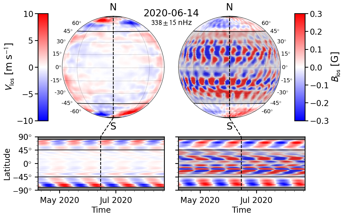
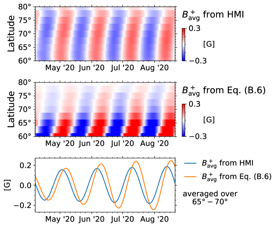
Figure 5 shows frequency-filtered images of the LOS Doppler velocity, and the LOS magnetic field derived from HMI observations. A bandpass filter centered at nHz with a full width of 30 nHz was applied to retain the mode. We emphasize that no spatial Fourier transform was applied. For , the structure of the mode is clearly visible at high latitudes, while little to no signal is present at lower latitudes. The data also shows the mode at high latitudes, but the lower latitudes display a plethora of signals associated with residual magnetic activity and not related to the mode. The bottom panels of Fig. 5 show synoptic maps of and , constructed by stacking the central meridian from bandpass-filtered images over time. The mode appears as inclined stripes in time-latitude space. A similar pattern was already visible in the synoptic maps of Fig. 1 in the absence of a frequency filter.
5 Discussion
We identified a coherent magnetic field oscillation at a frequency of nHz (with a frequency resolution of nHz) and a peak amplitude of about G in . This oscillation is associated with the high-latitude global inertial mode previously characterized in velocity data. The perturbations are predominantly symmetric across the equator, in contrast to the perturbations, which are primarily north-south antisymmetric. The magnetic field oscillations are most clearly observed at latitudes above during the recent solar minimum (2018–2022). The mode amplitude in peaks around 2012, during the rising phase of cycle 24, and again during 2020–2023, the rising phase of cycle 25. A time lag of approximately two years is observed between the trends in magnetic and velocity perturbations.
As outlined in a simple model in Appendix B, the amplitude of the magnetic oscillation during solar cycle minimum may be understood via the linearized induction equation, Eq. (10), whereby the radial magnetic field is advected by the hydrodynamic high-latitude mode. This simple model reproduces approximately the symmetric pattern at high latitudes with a maximum amplitude of G. The calculation assumes a dipolar background field magnetic field during solar minimum (Fig. 7). It would be interesting to repeat these calculations over different phases of the solar cycle using, e.g., a background magnetic field from a dynamo model.
Acknowledgements.
The observations were analyzed by SGH and Z-CL. The analytical model was derived by LG and Z-CL. SGH acknowledges funding from the Austrian Science Fund (FWF) Erwin-Schrödinger fellowship J-4560 and funding from the Research Council of Finland (Academy Fellowship): 370747 (RIB-Wind). We thank B. Proxauf and S. Good for valuable discussions. This work utilizes GONG data from NSO, which is operated by AURA under a cooperative agreement with NSF and with additional financial support from NOAA, NASA, and USAF. The HMI data used are courtesy of NASA/SDO and the HMI science team.References
- Bekki et al. (2022) Bekki, Y., Cameron, R. H., & Gizon, L. 2022, A&A, 662, A16
- Bekki et al. (2024) Bekki, Y., Cameron, R. H., & Gizon, L. 2024, Science Advances, 10, eadk5643
- Bogart et al. (2015) Bogart, R. S., Baldner, C. S., & Basu, S. 2015, ApJ, 807, 125
- Gizon et al. (2024) Gizon, L., Bekki, Y., Birch, A. C., et al. 2024, in IAU Symposium, Vol. 365, Dynamics of Solar and Stellar Convection Zones and Atmospheres, ed. A. V. Getling & L. L. Kitchatinov, 207–221
- Gizon et al. (2021) Gizon, L., Cameron, R. H., Bekki, Y., et al. 2021, A&A, 652, L6
- Hanasoge & Mandal (2019) Hanasoge, S. & Mandal, K. 2019, ApJ, 871, L32
- Harvey et al. (1996) Harvey, J. W., Hill, F., Hubbard, R. P., et al. 1996, Science, 272, 1284
- Hathaway et al. (2013) Hathaway, D. H., Upton, L., & Colegrove, O. 2013, Science, 342, 1217
- Liang & Gizon (2025) Liang, Z.-C. & Gizon, L. 2025, A&A, 695, A67 (LG25)
- Liang et al. (2019) Liang, Z.-C., Gizon, L., Birch, A. C., & Duvall, T. L. 2019, A&A, 626, A3
- Liu et al. (2017) Liu, Y., Hoeksema, J. T., Sun, X., & Hayashi, K. 2017, Sol. Phys., 292, 29
- Löptien et al. (2018) Löptien, B., Gizon, L., Birch, A. C., et al. 2018, Nature Astron., 2, 568
- Pesnell et al. (2012) Pesnell, W. D., Thompson, B. J., & Chamberlin, P. C. 2012, Sol. Phys., 275, 3
- Schou et al. (2012) Schou, J., Scherrer, P. H., Bush, R. I., et al. 2012, Sol. Phys., 275, 229
- Snodgrass (1984) Snodgrass, H. B. 1984, Sol. Phys., 94, 13
- Ulrich (1993) Ulrich, R. K. 1993, in Astronomical Society of the Pacific Conference Series, Vol. 40, IAU Colloq. 137: Inside the Stars, ed. W. W. Weiss & A. Baglin, 25–42
- Ulrich (2001) Ulrich, R. K. 2001, ApJ, 560, 466
Appendix A Phase of magnetic oscillations as a function of latitude
Appendix B Simplified model for magnetic field perturbations during cycle minimum
Let us consider the induction equation in an inertial frame,
| (8) |
Assuming background values of the magnetic field () and of the axisymmetric flow () during solar minimum, we wish to compute the perturbations to the magnetic field at the surface () caused by the fluctuating flow associated with a mode of oscillation. In the near-surface layers, the velocity field of a quasi-toroidal mode of oscillation is approximately horizontal and divergence free,
| (9) |
The magnetic field is assumed to be purely radial at the surface. We linearize the induction equation to obtain an equation for the magnetic field perturbation :
| (10) |
Taking the radial component of this equation, we have
| (11) |
where we used and .
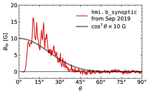
During solar minimum, the background field at the surface is approximately radial at the surface and independent of longitude, that is . As shown in Fig. 7, a reasonable model for the field is with G and . The background flow consists of rotation and the meridional flow, that is . We use the surface angular velocity profile from Snodgrass (1984) and the meridional flow profile m/s.
Next, we plug perturbations to the magnetic field of the form into Eq. (11) to obtain
| (12) |
We adopt a surface diffusivity of km2/s, consistent with the supergranulation. The RHS of the equation depends on the colatitudinal component of the high-latitude (HL1) mode velocity, , which we extract from HMI ring-diagram flow maps along the central meridian at the HL1 mode frequency. As a sanity check, we compute separately the left and side (LHS) of the equation using the observed as input, and the right hand side (RHS) of the equation using the observed . At latitudes above (i.e. above the critical latitude of the HL1 mode), we find that the two sides of the equation have comparable amplitudes. We also find that the diffusion and meridional flow terms on the LHS of Eq. (12) are negligible. This implies that a rough estimate for is
| (13) |
where is the critical colatitude given by . Figure 8 compares the line-of-sight projection of the fluctuating magnetic field derived from Eq. (13) to the observed during cycle minimum (also see Figure 1). Although the approximate model does not perfectly reproduce the observations (esp. the phase), it provides the correct order-of-magnitude estimate for the observed . We therefore conclude that the observed magnetic field perturbations at the surface are largely caused by the passive advection of the radial field by the HL1 mode (velocity ).