Guaranteed Noisy CP Tensor Recovery via Riemannian Optimization on the Segre Manifold

Ke Xu kxu6@nd.edu Department of Applied and Computational Mathematics and Statistics,
University of Notre Dame
Yuefeng Han yuefeng.han@nd.edu Department of Applied and Computational Mathematics and Statistics,
University of Notre Dame
Abstract

Recovering a low-CP-rank tensor from noisy linear measurements is a central challenge in high-dimensional data analysis, with applications spanning tensor PCA, tensor regression, and beyond. We exploit the intrinsic geometry of rank-one tensors by casting the recovery task as an optimization problem over the Segre manifold, the smooth Riemannian manifold of rank-one tensors. This geometric viewpoint yields two powerful algorithms: Riemannian Gradient Descent (RGD) and Riemannian Gauss-Newton (RGN), each of which preserves feasibility at every iteration. Under mild noise assumptions, we prove that RGD converges at a local linear rate, while RGN exhibits an initial local quadratic convergence phase that transitions to a linear rate as the iterates approach the statistical noise floor. Extensive synthetic experiments validate these convergence guarantees and demonstrate the practical effectiveness of our methods.

1 Introduction

Tensor decomposition, particularly the CP decomposition, has emerged as a powerful tool for analyzing high-dimensional data across diverse domains such as chemometrics, neuroscience, and recommendation systems (Tang and Li,, 2023; Frolov and Oseledets,, 2017; Bi etย al.,, 2021). Specifically, for an order-$d$ tensor $\mathcal{T}\in\mathbb{R}^{p_{1}\times\cdots\times p_{d}}$, the CP decomposition expresses it as a sum of rank-one tensors:

$\displaystyle\mathcal{T}=\sum_{i=1}^{r}\lambda_{i}u_{1,i}\otimes u_{2,i}\otimes\cdots\otimes u_{d,i},$ (1)

where $\otimes$ denotes tensor product, each factor $u_{k,i}\in\mathbb{R}^{p_{k}}$ vector with $\|u_{k,i}\|_{2}=1$, $r$ is the CP rank, and $\lambda_{i}\in\mathbb{R}$. Under mild identifiability conditions (e.g., Kruskalโ€™s criterion Kruskal, (1977)), this representation is essentially unique up to scaling and permutation, making it a widely adopted model in multi-way data analysis.

In practice, one often only observes noisy measurements of $\mathcal{T}$, for example

$$\mathcal{Y}=\mathcal{A}(\mathcal{T})+\mathcal{E},$$

where $\mathcal{A}$ is a linear observation operator (possibly compressive) and $\mathcal{E}$ denotes additive noise.

In this work, we address the problem of recovering the underlying low CP rank tensor $\mathcal{T}$ from noisy measurements. In particular, we perform optimization directly on the Segre manifold, a smooth Riemannian manifold composed of rank-one tensors. Utilizing Riemannian optimization techniques ensures that the iterates remain on the manifold, thereby preserving the structure of the CP model and achieving improved convergence properties over traditional Euclidean approaches (Kolda and Bader,, 2009).

Main contribution.

Our contributions can be summarized as follows:

  1. 1.

    We develop Riemannian Gradient Descent (RGD) and Riemannian Gauss-Newton (RGN) algorithms specifically tailored for noisy CP tensor estimation problems by directly optimizing on the Segre manifold.

  2. 2.

    We derive convergence guarantees for both the RGD and RGN methods in the noisy case and analyze the impact of the geometric properties on the convergence behavior.

  3. 3.

    Extensive experiments on simulation studies demonstrate that our algorithms yield robust and interpretable factor recovery under noisy conditions, outperforming traditional approaches.

1.1 Related Work

Classical methods for CP tensor decomposition, notably Alternating Least Squares (ALS) (Carroll and Chang,, 1970; Harshman etย al.,, 1970; Kolda and Bader,, 2009; Comon etย al.,, 2009), are widely used due to their conceptual simplicity and low per-iteration cost. However, ALS does not offer a general theoretical guarantee of convergence (Kolda and Bader,, 2009). Early theoretical work addressed this shortcoming under strong orthogonality assumptions, deriving convergence results for the orthogonal CP model (Anandkumar etย al., 2014a, ; Montanari and Richard,, 2014; Wang and Lu,, 2017). More recently, attention has turned to nonโ€orthogonal decompositions under soft incoherence assumptions. Anandkumar etย al., 2014b extended their ALS analysis to the nonโ€orthogonal case with random basis vectors on the sphere, and Sharan and Valiant (Sharan and Valiant,, 2017) proposed an โ€œorthogonalizedโ€ ALS variant. However, Sharan and Valiant, (2017) observed that its reliance on simultaneous diagonalization can be computationally inefficient.

More recently, manifold optimization techniques have shown promise for tensor estimation, particularly in the context of low-rank matrix and Tucker tensor decompositions (Boumal,, 2023; Luo and Zhang,, 2023, 2024). In these cases, tensors with fixed Tucker ranks form a Riemannian manifold, which provides a natural framework for optimization. The tangent space of this manifold admits a simple parametrization, facilitating efficient optimization (Kressner etย al.,, 2014). These methods have demonstrated significant improvements in tensor recovery, particularly in the noisy settings, by incorporating geometric properties of the manifold directly into the optimization process.

However, extending these Riemannian optimization methods to low CP rank tensor estimation presents unique challenges. In contrast to the Tucker decomposition, the CP model is inherently non-orthogonal, which leads to issues such as slower convergence, local minima, and increased computational complexity. While there have been attempts to address these issues, such as the work by Swijsen etย al., (2022), which introduced a Riemannian optimization approach for CP decomposition, a comprehensive theoretical analysis of the convergence properties of such methods remains an open question.

Our work bridges this gap by explicitly incorporating the geometric structure of the rank-one tensor space through Riemannian optimization techniques. Intuitively, a rank-one tensor can be viewed as a Tucker rank-one tensor, which sidesteps the non-orthogonality challenges in the CP model. Such greedy or rank-one updates are a natural procedure for CP tensor decomposition (Zhang and Golub,, 2001), and linear convergence rates for incoherent CP tensors are proved in Anandkumar etย al., 2014b ; Sun etย al., (2017). By leveraging recent advancements in manifold optimization, we develop algorithms that respect the intrinsic geometry of the CP model, while also providing robust convergence properties under noisy conditions. In particular, our work demonstrates that these techniques can improve upon traditional methods by ensuring feasibility at each iteration and offering better convergence guarantees, even in the presence of noise.

1.2 Organization

The remainder of this manuscript is organized as follows. In Sectionย 2, we introduce our framework and formulate the two core problems: tensor decomposition and tensor regression. Sectionย 3 presents our proposed Riemannian optimization algorithms and provides full algorithmic details. Sectionย 4 develops the theoretical analysis, including local convergence guarantees. In Sectionย 5, we report comprehensive experimental results. Finally, Sectionย 6 concludes the paper and outlines directions for future work. All detailed proofs are collected in the appendix.

2 Model and Problem Formulation

Our goal is to accurately recover the signal tensor $\mathcal{T}$, which admits the CP decomposition in (1), by solving an optimization problem that leverages the geometry of the Segre manifold. In particular, we address the following minimization problem:

$$\min_{(\mathcal{T}_{1},\dots,\mathcal{T}_{r})\,\in\,\operatorname{Seg}}\mathcal{L}(\{\mathcal{T}_{i}\}_{i=1}^{r})=\min_{(\mathcal{T}_{1},\dots,\mathcal{T}_{r})\,\in\,\operatorname{Seg}}\frac{1}{2}\Bigl\|\mathcal{Y}-\sum_{i=1}^{r}\mathcal{A}(\mathcal{T}_{i})\Bigr\|_{\mathrm{F}}^{2},$$ (2)

where the mapping $\mathcal{A}:\mathbb{R}^{p_{1}\times\cdots\times p_{d}}\to\mathbb{R}^{n}$ is a (possibly random) linear operator which allows for both complete and compressive observations of the tensor, $\operatorname{Seg}$ denotes the Segre manifold of rank-one tensors (Definitionย 1).

Previous work has largely focused on the estimation of the tensor factors by iterating across each mode of the tensor (Carroll and Chang,, 1970; Sharan and Valiant,, 2017). In contrast, our formulation directly iterates on the Segre manifold, the smooth Riemannian manifold composed of rank-one tensors. This intrinsic approach leverages the rank-one structure of each component, ensuring that the CP structure is preserved throughout the optimization. This formulation is sufficiently general to encompass a variety of applications, including:

Tensor Decomposition.

When the entire signal tensor ${\cal T}$ is observed, we simply take $\mathcal{A}=\mathrm{Id}:\mathbb{R}^{p_{1}\times\cdots\times p_{d}}\rightarrow\mathbb{R}^{p_{1}\times\cdots\times p_{d}}$. In this case, the problem in (2) becomes $\min_{\mathcal{T}_{i}\in\operatorname{Seg}}\frac{1}{2}\|\mathcal{Y}-\sum_{i=1}^{r}\mathcal{T}_{i}\|_{\mathrm{F}}^{2}$, which is exactly the classical CP decomposition in the presence of noise.

Tensor Regression.

In regression settings, we define the linear operator $\mathcal{A}:\mathbb{R}^{p_{1}\times\cdots\times p_{d}}\rightarrow\mathbb{R}^{n}$ by

$\displaystyle\mathcal{A}(\mathcal{T})=([\mathcal{A}(\mathcal{T})]_{1},...,[\mathcal{A}(\mathcal{T})]_{n})^{\top},\;[\mathcal{A}(\mathcal{T})]_{m}=\langle\mathcal{X}_{m},\mathcal{T}\rangle,\quad m=1,2,\dots,n,$

where $\{\mathcal{X}_{m}\}_{m=1}^{n}$ are known tensor covariates and $\langle\cdot,\cdot\rangle$ denotes the ambient inner product in the tensor space. We assume design tensors $\mathcal{X}_{m}$ and noise tensors $\mathcal{E}_{m}$ are i.i.d. Gaussian, and that $\mathcal{X}_{m}$ and $\mathcal{E}_{m}$ are independent. In particular, we assume that ${\rm Cov}(\mathcal{E}_{m})=\sigma^{2}I_{\prod_{l=1}^{d}p_{l}}$. Under these assumptions, the adjoint operator $\mathcal{A}^{*}$ satisfies $\mathcal{A}^{*}(\mathcal{Y})={1/(n\sigma^{2})}\sum_{m=1}^{n}y_{m}\mathcal{X}_{m}$ and $\mathcal{A}^{*}\mathcal{A}(\mathcal{T})={1/(n\sigma^{2})}\sum_{m=1}^{n}\langle\mathcal{X}_{m},\mathcal{T}\rangle\mathcal{X}_{m}$.

3 Method

In this section, we present two algorithms, Riemannian Gradient Descent (RGD) and Riemannian Gauss-Newton (RGN), tailored for noisy CP tensor recovery. Rather than optimizing in the full ambient space, both methods update all $r$ rank-one tensor factors simultaneously on the Segre manifold.

3.1 Background and Preliminaries

This subsection introduces the foundational concepts of our proposed Riemannian tensor decomposition framework.

Given a tensor $\mathcal{T}\in\mathbb{R}^{p_{1}\times p_{2}\times\cdots\times p_{d}}$, a (nonzero) rank-one tensor is of the form $\mathcal{T}=u_{1}\otimes u_{2}\otimes\cdots\otimes u_{d},$ with $u_{k}\in\mathbb{R}^{p_{k}}\setminus\{0\}$ for $k=1,\ldots,d$. The collection of projective classes of rank-one tensors forms the Segre variety in algebraic geometry (Landsberg,, 2011). When one instead considers the set of nonzero rank-one tensors in the ambient space $\mathbb{R}^{p_{1}\times\cdots\times p_{d}}$ endowed with the Frobenius metric, this set becomes a smooth Riemannian submanifold called the Segre manifold (denoted by $\operatorname{Seg}$). The geometry of the Segre manifold is summarized in Jacobsson etย al., (2024).

Definition 1 (Segre Manifold).

The Segre manifold is the set of all nonzero rank-one tensors in the ambient space $\mathbb{R}^{p_{1}\times\cdots\times p_{d}}$,

$$\operatorname{Seg}\;=\;\Big\{\,u_{1}\otimes u_{2}\otimes\cdots\otimes u_{d}:u_{l}\in\mathbb{R}^{p_{l}}\setminus\{0\},\ \forall l\in[d]\,\Big\}.$$

It is a smooth embedded submanifold of $\mathbb{R}^{\prod_{l\in[d]}p_{l}}\setminus\{0\}$ of dimension $\dim(\operatorname{Seg})\;=\;1+\sum_{l\in[d]}(p_{l}-1)$.

Remark 1.

An equivalent parameterization of Segre manifold is given by the following diffeomorphism:

$$\operatorname{Seg}\ \cong\ \big(\mathbb{R}^{+}\times\mathbb{S}^{p_{1}-1}\times\cdots\times\mathbb{S}^{p_{d}-1}\big)\big/G,$$

where $G=\{(\varepsilon_{1},\dots,\varepsilon_{d})\in\{\pm 1\}^{d}:\prod_{k=1}^{d}\varepsilon_{k}=1\}$ acts by simultaneous sign flips. This quotient accounts for the sign ambiguity, since different sign patterns of the factor vectors can represent the same tensor. Projectivizing $\mathcal{S}$ (i.e., identifying tensors up to nonzero scalar multiples) recovers the classical Segre variety in algebraic geometry (Landsberg,, 2011).

We therefore optimize over $r$-tuples of rank-one tensors, each of which lies on the Segre manifold ($\operatorname{Seg}$). To ensure these components remain distinguishable, we impose an incoherence condition among them, effectively acting as a soft-orthogonality constraint. Let $[n]$ denote the set $\{1,2,\ldots,n\}$.

Assumption 1.

Assume for any mode $l\in[d]$, the following incoherence holds:

ฮผl=plโ‹…maxi,jโˆˆ[r],iโ‰ jโก|โŸจul,i,ul,jโŸฉ|2.\mu_{l}=p_{l}\cdot\max_{\begin{subarray}{c}i,j\in[r],i\neq j\end{subarray}}|\langle u_{l,i},u_{l,j}\rangle|^{2}.

Furthermore, let $\eta=\max_{l\in[d]}\sqrt{\mu_{l}/p_{l}}$.

This assumption is standard in the CP tensor estimation literature Anandkumar etย al., 2014b ; Cai etย al., (2020, 2022). Moreover, Lemma 2 of Anandkumar etย al., 2014b shows that if $\{u_{l,i}\}_{l\in[d],i\in[r]}$ are drawn i.i.d. from the unit sphere $\SS^{p_{l}-1}$, then with high probability maxiโ‰ jโก{|โŸจul,i,ul,jโŸฉ|}โ‰1/pl\max_{i\neq j}\{|\langle u_{l,i},u_{l,j}\rangle|\}\asymp 1/\sqrt{p_{l}}. Most existing analyses rely on such asymptotically vanishing incoherence, i.e., $\eta=\Omega\!\left(1/{\sqrt{\max_{l\in[d]}p_{l}}}\right)$. In contrast, our analysis only requires $\eta$ to be bounded but sufficiently small, rather than decaying with dimension.

Any CP tensor of rank $r$ admits a Tucker representation with multilinear rank $(r,\cdots,r)$. In the special case of a rank-one tensor, the Tucker and CP parameterizations coincide. Hence, by optimizing directly over the product of $r$ rank-one manifolds, rather than over each of the $d$ mode factors of a rank-$r$ tensor, we fully leverage the intrinsic rank-one structure and seamlessly handle non-orthogonal factor interactions.

3.2 Riemann Gradient Descent on Segre Manifold

Standard gradient descent in Euclidean space ignores the underlying manifold structure; instead, we employ Riemannian gradient descent. At each iteration $t$, for a rank-one tensor ${\cal T}_{i}\in\operatorname{Seg}$ and its tangent space $\mathbb{T}_{i}$, we compute the Riemannian update by first projecting the Euclidean gradient onto the tangent space and then retracting back onto the manifold

$\displaystyle\mathcal{T}_{i}^{(t+1)}=\mathcal{R}_{\mathcal{T}_{i}^{(t)}}\Big(-\alpha_{t}\,\mathcal{P}_{\mathbb{T}_{i}^{(t)}}\Big(\nabla_{\mathcal{T}_{i}}\mathcal{L}\big(\{\mathcal{T}_{i}^{(t)}\}_{i=1}^{r}\big)\Big)\Big),$

where $\alpha_{t}$ is the step size at iteration $t$, $\nabla_{\mathcal{T}_{i}}\mathcal{L}$ is the partial gradient of the loss, $\mathcal{P}_{\mathbb{T}_{i}^{(t)}}$ denotes projection onto the tangent space at $\mathcal{T}_{i}^{(t)}$, and $\mathcal{R}$ is a retraction from the tangent space back to the Segre manifold.

Tangent Space of the Segre Manifold.

The tangent space captures the manifoldโ€™s local linear structure around a point. For a rank-one tensor $\mathcal{T}_{i}=u_{1,i}\otimes u_{2,i}\otimes\cdots\otimes u_{d,i}$ in $r$ rank-one components of $\mathcal{T}$, its tangent space $\mathbb{T}_{i}\operatorname{Seg}$ consists of all first-order variations in each factor direction. Concretely, every tangent vector $\xi_{i}\in\mathbb{T}_{i}$ admits the decomposition

$$\xi_{i}=\sum_{k=1}^{d}u_{1,i}\otimes\cdots\otimes u_{k-1,i}\otimes h_{k,i}\otimes u_{k+1,i}\otimes\cdots\otimes u_{d,i},$$

where each $h_{k,i}\in\mathbb{R}^{p_{k}}$ represents an arbitrary infinitesimal perturbation of the $k$-th factor.

For each mode $k$, define the orthogonal projector $\mathcal{P}_{k,i}=u_{k,i}u_{k,i}^{\top}$, which projects $\mathbb{R}^{p_{k}}$ onto the span of $u_{k,i}$, and its complement $\mathcal{P}_{k,i}^{\perp}=I_{p_{k}}-u_{k,i}u_{k,i}^{\top}$. Denote by $\hbox{\rm mat}_{k}(\mathcal{T}_{i})$ the mode-$k$ matricization of $\mathcal{T}_{i}\in\mathbb{R}^{p_{1}\times p_{2}\times\cdots\times p_{d}}$. Minimizing the squared Frobenius norm $\|\widetilde{\mathcal{T}}-\xi_{i}\|_{\mathrm{F}}^{2}$ subject to $\xi_{i}\in\mathbb{T}_{i}$ yields the following full projection of an arbitrary tensor $\widetilde{{\cal T}}$ onto the tangent space at $\mathcal{T}_{i}$ is

ฮพi=๐’ซ๐•‹iโ€‹(๐’ฏ~)=โˆ‘k=1d๐’ซk,iโŸ‚โ€‹matkโ€‹(๐’ฏ~)โŠ—lโ‰ k๐’ซl,i+๐’ฏ~ร—lโˆˆ[d]๐’ซl,i.\xi_{i}=\mathcal{P}_{\mathbb{T}_{i}}(\widetilde{{\cal T}})=\sum_{k=1}^{d}\mathcal{P}_{k,i}^{\perp}\hbox{\rm mat}_{k}(\widetilde{{\cal T}})\otimes_{l\neq k}\mathcal{P}_{l,i}+\widetilde{{\cal T}}\times_{l\in[d]}\mathcal{P}_{l,i}. (3)

Retraction

A descent step in the tangent space typically produces an update off the manifold, so we apply a retraction to map it back onto the Segre manifold. Popular retractions include the truncated higher-order singular value decomposition (T-HOSVD) Deย Lathauwer etย al., (2000) and its sequential version (ST-HOSVD) Vannieuwenhoven etย al., (2012). More recent work has even derived explicit geodesics and thus the exponential map on the Segre manifold Swijsen etย al., (2022); Jacobsson etย al., (2024). For a comprehensive overview of these geometric operators, see Boumal, (2023). In this paper, we adopt the T-HOSVD retraction, leaving alternative mappings to future work.

3.3 Riemann Gauss-Newton on Segre Manifold

Although Riemannian gradient descent is conceptually simple, its convergence can be slow, especially for large-scale problems or when high accuracy is needed. Incorporating second-order information offers a powerful remedy. The Riemannian Gauss-Newton method Luo and Zhang, (2023), tailored to nonlinear least-squares, provides an efficient approximation to the full Riemannian Newton step.

Concretely, RGN seeks a tangent-space update $s_{k}\in\mathbb{T}_{\mathcal{T}_{k}}$ satisfying the Gauss-Newton equation

$$\operatorname{Hess}\mathcal{L}(\{\mathcal{T}_{i}\}_{i=1}^{r})[s_{k}]=-\operatorname{grad}\mathcal{L}(\{\mathcal{T}_{i}\}_{i=1}^{r}),$$

where $\mathcal{L}(\{\mathcal{T}_{i}\}_{i=1}^{r})=\frac{1}{2}\|\mathcal{Y}-\sum_{i=1}^{r}\mathcal{A}(\mathcal{T}_{i})\|_{\mathrm{F}}^{2}$. By approximating the true Hessian with the Gauss-Newton Hessian, RGN captures essential curvature information at low cost, yielding faster convergence and higher accuracy in noisy CP tensor recovery.

The RGN algorithm enforces feasibility by projecting each search direction onto the tangent space via the projection $\mathcal{P}_{\mathbb{T}_{i}^{(t)}}$, and then retracting back onto the Segre manifold. Importantly, this approach still solves a least-squares problem, but in a drastically lower-dimensional space: the tangent-space formulation has only $1+\sum_{l\in[d]}(p_{l}-1)$ degrees of freedom, versus $\prod_{l\in[d]}p_{l}$ parameters in the original ambient tensor space $\mathbb{R}^{p_{1}\times p_{2}\times\cdots\times p_{l}}$.

Algorithm 1 Riemannian Gradient Descent for CP Tensor Estimation

Input: Observation $\mathcal{Y}=\sum_{i=1}^{r}\mathcal{A}(\mathcal{T}_{i})+\mathcal{E}\in\mathbb{R}^{n}$, linear operator $\mathcal{A}:\mathbb{R}^{p_{1}\times p_{2}\times\cdots\times p_{d}}\rightarrow\mathbb{R}^{n}$, target CP rank $r$, and initial rank-one tensor estimates $\{\mathcal{T}_{i}^{(0)}\}_{i=1}^{r}$.

1:โ€‚for $t=0,1,\dots,t_{\max}-1$ do
2:โ€ƒโ€‚for $i=1,\dots,r$ do
3:โ€ƒโ€ƒโ€‚(RGD Update) Update
$$\mathcal{T}_{i}^{(t+1)}=\mathcal{R}_{\mathcal{T}_{i}^{(t)}}\Big(\mathcal{T}_{i}^{(t)}-\alpha_{t}\mathcal{P}_{\mathbb{T}_{i}^{(t)}}\mathcal{A}^{*}\big(\sum_{i=1}^{r}\mathcal{A}(\mathcal{T}_{i}^{(t)})-\mathcal{Y}\big)\Big),$$
where $\alpha_{t}$ is the step size, ${\cal A}^{*}(\cdot)$ is the adjoint measurement operator, $\mathcal{P}_{\mathbb{T}_{i}^{(t)}}(\cdot)$ projects onto the tangent space $\mathbb{T}_{i}^{(t)}$ at $\mathcal{T}_{i}^{(t)}$. Writing $\mathcal{T}_{i}^{(t)}=\lambda_{i}^{(t)}u_{1,i}^{(t)}\otimes\cdots\otimes u_{d,i}^{(t)}$ with $u_{l,i}^{(t)}\in\SS^{p_{l}-1}$ for any $l\in[d],i\in[r]$, the formula of projection onto tangent space can be found in (3) and $\mathcal{R}_{\mathcal{T}_{i}^{(t)}}$ denotes our chosen retraction (here, T-HOSVD).
4:โ€ƒโ€‚end for
5:โ€‚end for

Output: $\{\mathcal{T}_{i}^{(t_{\max})}\}_{i=1}^{r}$.

Algorithm 2 Riemannian Gauss-Newton for CP Tensor Estimation

Input: Observation $\mathcal{Y}=\sum_{i=1}^{r}\mathcal{A}(\mathcal{T}_{i})+\mathcal{E}\in\mathbb{R}^{n}$, linear operator $\mathcal{A}:\mathbb{R}^{p_{1}\times p_{2}\times\cdots\times p_{d}}\rightarrow\mathbb{R}^{n}$, target CP rank $r$, and initial rank-one tensor estimates $\{\mathcal{T}_{i}^{(0)}\}_{i=1}^{r}$.

1:โ€‚for $t=0,1,\dots,t_{\max}-1$ do
2:โ€ƒโ€‚for $i=1,\dots,r$ do
3:โ€ƒโ€ƒโ€‚(RGN Update) Update
$$\mathcal{T}_{i}^{(t+1)}=\mathcal{R}_{\mathcal{T}_{i}^{(t)}}\Big(\mathcal{T}_{i}^{(t)}-\big(\mathcal{P}_{\mathbb{T}_{i}^{(t)}}\mathcal{A}^{*}\mathcal{A}\mathcal{P}_{\mathbb{T}_{i}^{(t)}}\big)^{-1}\mathcal{P}_{\mathbb{T}_{i}^{(t)}}\mathcal{A}^{*}\big(\sum_{i=1}^{r}\mathcal{A}(\mathcal{T}_{i}^{(t)})-\mathcal{Y}\big)\Big),$$
where ${\cal A}^{*}(\cdot)$ is the adjoint measurement operator, $\mathcal{P}_{\mathbb{T}_{i}^{(t)}}(\cdot)$ projects onto the tangent space $\mathbb{T}_{i}^{(t)}$ at $\mathcal{T}_{i}^{(t)}$ (see (3)), and $\mathcal{R}_{\mathcal{T}_{i}^{(t)}}$ denotes our chosen retraction (here, T-HOSVD)..
4:โ€ƒโ€‚end for
5:โ€‚end for

Output: $\{\mathcal{T}_{i}^{(t_{\max})}\}_{i=1}^{r}$.

4 Theoretical Analysis

4.1 Convergence Analysis of Riemann Optimization

In this subsection, we present a deterministic convergence analysis for both RGD and RGN, as stated in Theorems 4.1 and 4.2, respectively. Even in the presence of noise, our results guarantee local convergence by exploiting the Segre manifoldโ€™s intrinsic geometry to bound the distance between each iterate and its true rank-one component.

Theorem 4.1 (Local Convergence of RGD).

Suppose that for each $i\in[r]$, the current estimate $\mathcal{T}_{i}^{(t)}$ at iteration $t$ satisfies $\langle\mathcal{T}_{i}^{(t)},\mathcal{T}_{i}\rangle\geq 0$, where $\mathcal{T}_{i}$ is the true rank-one tensor. Define $\varepsilon^{(t)}=\max_{i\in[r]}(\|\mathcal{T}_{i}^{(t)}-\mathcal{T}_{i}\|_{\mathrm{F}}/\lambda_{i})$ as the relative Frobenius error of the rank-one component tensor at iteration $t$, where $\lambda_{i}$โ€™s are the component weights of the CP decomposition, and let $\eta$ be the incoherence parameter defined in Assumptionย 1. Then, for all $t\geqslant 0$, the next error $\varepsilon^{(t+1)}$ satisfies a three-term bound of the form

$\displaystyle\varepsilon^{(t+1)}$
$\displaystyle\leqslant$ (d+1)โ€‹(maxiโˆˆ[r]โกโ€–๐’ซ๐•‹i(t)โ€‹(Iโˆ’ฮฑtโ€‹๐’œโˆ—โ€‹๐’œ)โ€‹๐’ซ๐•‹i(t)โ€–F+(rโˆ’1)โ€‹ฮฑtโ€‹ฮบโ€‹maxi,jโˆˆ[r],iโ‰ jโกโ€–๐’ซ๐•‹i(t)โ€‹๐’œโˆ—โ€‹๐’œโ€‹๐’ซ๐•‹i(t)โŸ‚โ€‹๐’ซ๐•‹j(t)โ€–)โ‹…ฮต(t)โŸfirst-order contraction\displaystyle\underbrace{(\sqrt{d}+1)\big(\max_{i\in[r]}\big\|\mathcal{P}_{\mathbb{T}_{i}^{(t)}}(I-\alpha_{t}\mathcal{A}^{*}\mathcal{A})\mathcal{P}_{\mathbb{T}_{i}^{(t)}}\big\|_{\mathrm{F}}+(r-1)\alpha_{t}\kappa\max_{i,j\in[r],i\neq j}\big\|\mathcal{P}_{\mathbb{T}_{i}^{(t)}}\mathcal{A}^{*}\mathcal{A}\mathcal{P}_{\mathbb{T}_{i}^{(t)}}^{\perp}\mathcal{P}_{\mathbb{T}_{j}^{(t)}}\big\|\big)\cdot\varepsilon^{(t)}}_{\text{first-order contraction}}
$\displaystyle+$ $\displaystyle\underbrace{(\sqrt{d}+1)^{3}\Big[1+2r\alpha_{t}\cdot\max_{i\in[r]}\sup_{V\in\operatorname{Seg}}\big\|\big(\mathcal{P}_{\mathbb{T}_{i}^{(t)}}\mathcal{A}^{*}\mathcal{A}\mathcal{P}_{\mathbb{T}_{i}^{(t)}}\big)^{-1}\mathcal{A}^{*}\mathcal{A}\mathcal{P}_{\mathbb{T}_{i}^{(t)}}^{\perp}V\big\|\Big]\cdot\big(\varepsilon^{(t)}\big)^{2}}_{\text{second-order contraction}}$
$\displaystyle+$ $\displaystyle\underbrace{2r\alpha_{t}(\sqrt{d}+1)^{3}\max_{i\in[r]}\big\|\mathcal{P}_{\mathbb{T}_{i}^{(t)}}\mathcal{A}^{*}\mathcal{AP}_{\mathbb{T}_{i}^{(t)}}\big\|\cdot\big\{(\varepsilon^{(t)}+\eta)^{d-1}+\varepsilon^{(t)}\big\}\cdot\varepsilon^{(t)}}_{\text{second-order contraction}}+\underbrace{(\sqrt{d}+1)\cdot\alpha_{t}\max_{i\in[r]}\frac{\big\|\mathcal{P}_{\mathbb{T}_{i}^{(t)}}(\mathcal{A}^{*}\mathcal{E})\big\|_{\mathrm{F}}}{\lambda_{i}}}_{\text{noise term}}.$
Theorem 4.2 (Local Convergence of RGN).

Assume the same conditions in Theoremย 4.1, with $\varepsilon^{(t)}=\max_{i\in[r]}\|\mathcal{T}_{i}^{(t)}-\mathcal{T}_{i}\|_{\mathrm{F}}/\lambda_{i}$. The convergence of RGN is given by

$\displaystyle\varepsilon^{(t+1)}$
$\displaystyle\leqslant$ (d+1)โ€‹(rโˆ’1)โ‹…maxiโ‰ j,i,jโˆˆ[r]โกโ€–(๐’ซ๐•‹i(t)โ€‹๐’œโˆ—โ€‹๐’œโ€‹๐’ซ๐•‹i(t))โˆ’1โ€‹๐’œโˆ—โ€‹๐’œโ€‹๐’ซ๐•‹i(t)โŸ‚โ€‹๐’ซ๐•‹j(t)โ€–โ‹…ฮต(t)โŸfirst-order contraction\displaystyle\underbrace{(\sqrt{d}+1)(r-1)\cdot\max_{i\neq j,i,j\in[r]}\big\|\big(\mathcal{P}_{\mathbb{T}_{i}^{(t)}}\mathcal{A}^{*}\mathcal{A}\mathcal{P}_{\mathbb{T}_{i}^{(t)}}\big)^{-1}\mathcal{A}^{*}\mathcal{A}\mathcal{P}_{\mathbb{T}_{i}^{(t)}}^{\perp}\mathcal{P}_{\mathbb{T}_{j}^{(t)}}\big\|\cdot\varepsilon^{(t)}}_{\text{first-order contraction}}
$\displaystyle+$ $\displaystyle\underbrace{2(\sqrt{d}+1)^{3}\Big(1+2(r-1)\cdot\max_{i\in[r]}\sup_{V\in\operatorname{Seg}}\big\|\big(\mathcal{P}_{\mathbb{T}_{i}^{(t)}}\mathcal{A}^{*}\mathcal{A}\mathcal{P}_{\mathbb{T}_{i}^{(t)}}\big)^{-1}\mathcal{A}^{*}\mathcal{A}\mathcal{P}_{\mathbb{T}_{i}^{(t)}}^{\perp}V\big\|_{\mathrm{F}}\Big)\cdot\big[(\varepsilon^{(t)}+\eta)^{d-1}+\varepsilon^{(t)}\big]\cdot\varepsilon^{(t)}}_{\text{second-order contraction}}$
$\displaystyle+$ $\displaystyle\underbrace{(\sqrt{d}+1)\max_{i\in[r]}\frac{\big\|\big(\mathcal{P}_{\mathbb{T}_{i}^{(t)}}\mathcal{A}^{*}\mathcal{A}\mathcal{P}_{\mathbb{T}_{i}^{(t)}}\big)^{-1}\mathcal{A}^{*}(\mathcal{E})\big\|_{\mathrm{F}}}{\lambda_{i}}}_{\text{noise term}}.$

Although both RGD and RGN feature a first-order error term proportional to $\varepsilon^{(t)}$, RGN attains second-order convergence by incorporating curvature information. The key quantities

$$\sup_{V\in\operatorname{Seg}}\big\|\big(\mathcal{P}_{\mathbb{T}_{i}^{(t)}}\mathcal{A}^{*}\mathcal{A}\mathcal{P}_{\mathbb{T}_{i}^{(t)}}\big)^{-1}\mathcal{A}^{*}\mathcal{A}\mathcal{P}_{\mathbb{T}_{i}^{(t)}}^{\perp}\mathcal{P}_{\mathbb{T}_{\mathbb{T}_{j}^{(t)}}}V\big\|\ \ \text{and}\ \ \sup_{V\in\operatorname{Seg}}\big\|\big(\mathcal{P}_{\mathbb{T}_{i}^{(t)}}\mathcal{A}^{*}\mathcal{A}\mathcal{P}_{\mathbb{T}_{i}^{(t)}}\big)^{-1}\mathcal{A}^{*}\mathcal{A}\mathcal{P}_{\mathbb{T}_{i}^{(t)}}^{\perp}V\big\|$$

control the higher-order behavior. In the noiseless CP decomposition setting, these norms vanish exactly, hence quadratic convergence. In tensor regression, they remain small because ${\cal A}$ projects onto a low-dimensional subspace, and the operators $\mathcal{A}\mathcal{P}_{\mathbb{T}_{i}^{(t)}}$ and $\mathcal{A}\mathcal{P}_{\mathbb{T}_{i}^{(t)}}^{\perp}\mathcal{P}_{\mathbb{T}_{\mathbb{T}_{j}^{(t)}}}$ are nearly independent, thereby ensuring the first-order terms are properly controlled.

Furthermore, many existing CP tensor estimation methods (Anandkumar etย al., 2014a, ; Anandkumar etย al., 2014b, ) require the incoherence parameter $\eta$ to decay at the rate $\sqrt{1/p_{l}}$. In contrast, our approach only requires $\eta$ to remain bounded (it does not have to vanish) by a sufficiently small constant to guarantee local convergence.

4.2 Implications in Statistics and Machine Learning

In this section, we examine the performance of RGD and RGN in two specific machine learning problems: CP tensor decomposition and tensor regression. In the Appendix, we provide more general versions of these corollaries. Let $\lfloor x\rfloor$ be the greatest integer less than or equal to $x$. Define $p^{*}=\prod_{l=1}^{d}p_{l}$ and $\bar{p}=\max_{l\in[d]}p_{l}$. Without loss of generality, we assume the component weights $\lambda_{1}\geq\lambda_{2}\geq\cdots\geq\lambda_{r}$ and let $\kappa=\lambda_{1}/\lambda_{r}$ be the condition number.

Tensor Decomposition.

Consider the noisy CP decomposition model

$$\mathcal{Y}=\mathcal{T}+\mathcal{E}\;\in\;\mathbb{R}^{p_{1}\times\cdots\times p_{d}},$$

where

$$\mathcal{T}\;=\;\sum_{i=1}^{r}\lambda_{i}\,u_{i,1}\otimes\cdots\otimes u_{i,d}\quad\text{and}\quad\operatorname{vec}(\mathcal{E})\sim\mathcal{N}\bigl(0,\Sigma_{p^{*}}\bigr),$$

and the noise covariance satisfies $\underline{\sigma}\,I_{p^{*}}\;\preceq\;\Sigma_{p^{*}}\;\preceq\;\overline{\sigma}\,I_{p^{*}}$. Under incoherence condition and a suitably small initialization error obtainable via spectral methods, such as HOSVD (Deย Lathauwer etย al.,, 2000) and CPCA (Han and Zhang,, 2022) or random initialization), we establish the following convergence guarantees for RGD and RGN.

Corollary 4.1 (Convergence rate of RGD for Tensor CP decomposition).

Let $\varepsilon^{(t)}=\max_{i\in[r]}(\|\mathcal{T}_{i}^{(t)}-\mathcal{T}_{i}\|_{\mathrm{F}}/\lambda_{i})$. Assume that $1-1/6\cdot(\sqrt{d}+1)\leqslant\alpha_{t}\leqslant 1$, $\varepsilon^{(0)}\leqslant 1/(8(\sqrt{d}+1)^{3}\cdot(1+3\kappa r))$ and $\alpha_{t}\eta^{d-1}\leqslant 1/(12\kappa r\cdot(\sqrt{d}+1)^{3})$ with $\eta$ in Assumptionย 1. Then, with probability at least $1-\exp(-c\bar{p})$, it follows that, for positive constants $c$ and $C$,

$\displaystyle\varepsilon^{(t)}\leqslant 2^{-t}\varepsilon^{(0)}+C\overline{\sigma}(\sqrt{d}+1)\ \sqrt{\bar{p}r}/\lambda_{r}.$
Corollary 4.2 (Convergence rate of RGN for Tensor CP decomposition).

Let $\varepsilon^{(t)}=\max_{i\in[r]}(\|\mathcal{T}_{i}^{(t)}-\mathcal{T}_{i}\|_{\mathrm{F}}/\lambda_{i})$. Assume that $\eta^{d-1}\leqslant\varepsilon^{(0)}\leqslant 1/(12(\sqrt{d}+1)^{3})$ with $\eta$ in Assumptionย 1.Then, with probability at least $1-\exp(-c\bar{p})$, it follows that, for positive constants $c$ and $C$,

$$\varepsilon^{(t)}\leqslant\begin{cases}2^{-2^{t}}\varepsilon^{(0)}+C(\sqrt{d}+1)\overline{\sigma}\sqrt{\bar{p}r}/\lambda_{r},&0\leqslant t\leqslant t^{*}=\lfloor-c(d-1)\log\eta\rfloor,\\ 2^{-(t-t^{*})}\varepsilon^{(t^{*})}+C(\sqrt{d}+1)\overline{\sigma}\sqrt{\bar{p}r}/\lambda_{r},&t\geqslant t^{*}.\end{cases}$$

Although our proofs of linear and quadratic convergence do not themselves invoke any signalโ€toโ€noise ratio (SNR) or sampleโ€size assumptions, such conditions are nonetheless required by the chosen initialization method. A typical spectral initialization, such as T-HOSVD (Deย Lathauwer etย al.,, 2000) and CPCA (Han and Zhang,, 2022) requires SNR ratio $\lambda_{r}=\Omega(\bar{p}^{d/4})$ in tensor CP decomposition and sample size $n/\lambda_{r}=\Omega(\bar{p}^{d/2})$ in tensor regression.

Tensor Regression.

In the tensor-regression setting, we observe

$$y_{i}=\langle\mathcal{X}_{i},\mathcal{T}\rangle+\mathcal{E}_{i},$$

for $i=1,2,\cdots,n$, where the design $\{\mathcal{X}_{i}\}_{i=1}^{n}$ are i.i.d. Gaussian tensors and satisfy $\operatorname{Cov}(\hbox{\rm vec}(\mathcal{X}_{i}))=\sigma^{2}I_{p^{*}}$. However, our results extend to sub-Gaussian design tensors. In the sub-Gaussian case, one shows (via a tensor restricted isometry property, see Definition 1 and Proposition 1 of Luo and Zhang, (2024)) that the design also approximately preserves the norm of any low-rank signal tensor, just as the Gaussian ensemble does. In the following corollaries, $\gamma$ can be viewed as a constant that quantifies the restricted isometry property. Furthermore, we assume that the additive noise $\mathcal{E}_{i}$โ€™s are independently Gaussian and $\sigma_{\xi}\,I_{n}\;\preceq\;\operatorname{Cov}\left(\mathcal{E}\right)\;\preceq\;\overline{\sigma}_{\xi}\,I_{n}$

Remark 2.

By assuming $\operatorname{Cov}(\hbox{\rm vec}(\mathcal{X}_{m}))=\sigma^{2}I_{p^{*}}$, we indeed assume that entries of each $\mathcal{X}_{m}$ are i.i.d. More generally, let $\Sigma=\operatorname{Cov}(\hbox{\rm vec}(\mathcal{X}_{m}))$. Then, the adjoint operator can be written as $\mathcal{A}^{*}(\mathcal{Y})=1/n\sum_{m=1}^{n}y_{m}\hbox{\rm vec}^{-1}(\Sigma^{-1}\hbox{\rm vec}(\mathcal{X}_{m}))$. In practice, estimating $\operatorname{Cov}(\hbox{\rm vec}(\mathcal{X}_{m}))$ with a general structure typically requires additional structural assumptions, which are beyond the scope of this paper.

Corollary 4.3 (Convergence rate of RGD for CP tensor regression).

Let $\varepsilon^{(t)}=\max_{i\in[r]}(\|\mathcal{T}_{i}^{(t)}-\mathcal{T}_{i}\|_{\mathrm{F}}/\lambda_{i})$ and $\gamma=\sqrt{\bar{p}/n}$ be sufficiently small. Assume that $1-1/6\cdot(\sqrt{d}+1)\leqslant\alpha_{t}\leqslant 1-\delta$, where $\delta$ is a constant depending on $\gamma$, $\varepsilon^{(0)}\leqslant 1/(8(\sqrt{d}+1)^{3}\cdot(1+3\kappa r))$ and $\alpha_{t}\eta^{d-1}\leqslant 1/(12\kappa r\cdot(\sqrt{d}+1)^{3})$ with $\eta$ in Assumptionย 1. Then, with probability at least $1-\exp(-c\bar{p})$, it follows that, for positive constants $c$ and $C$,

$\displaystyle\varepsilon^{(t)}\leqslant 2^{-t}\varepsilon^{(0)}+C(\sqrt{d}+1)\overline{\sigma}_{\xi}\sqrt{\bar{p}r}/(\sigma\lambda_{r}\sqrt{n}).$
Corollary 4.4 (Convergence rate of RGN for CP tensor regression).

Let $\varepsilon^{(t)}=\max_{i\in[r]}(\|\mathcal{T}_{i}^{(t)}-\mathcal{T}_{i}\|_{\mathrm{F}}/\lambda_{i})$ and $\gamma=\sqrt{\bar{p}/n}$ be sufficiently small. Assume that $\eta^{d-1}\leqslant\varepsilon^{(0)}\leqslant 1/(8(\sqrt{d}+1)^{3})$ with $\eta$ in Assumptionย 1. Then, with probability at least $1-\exp(-c\bar{p})$, it follows that, for positive constants $c$ and $C$,

$$\varepsilon^{(t)}\leqslant\begin{cases}2^{-2^{t}}\varepsilon^{(0)}+C(\sqrt{d}+1)\overline{\sigma}_{\xi}\sqrt{\bar{p}r}/(\sigma\lambda_{r}\sqrt{n}),&0\leqslant t\leqslant t^{*}=\lfloor-c(d-1)\log(\eta)\rfloor,\\ 2^{-(t-t^{*})}\varepsilon^{(t^{*})}+C(\sqrt{d}+1)\overline{\sigma}_{\xi}\sqrt{\bar{p}r}/(\sigma\lambda_{r}\sqrt{n}),&t\geqslant t^{*}.\end{cases}$$
Remark 3.

In Corollaries 4.2 and 4.4, the RGN algorithm exhibits two-phase convergence driven by the recursion for the normalized error

$$\varepsilon^{(t+1)}\leqslant\underbrace{C_{1}[(\varepsilon^{(t)}+\eta)^{d-1}+\varepsilon^{(t)}]\varepsilon^{(t)}}_{\text{linear + quadratic term }}+\underbrace{C_{2}\mathcal{E}(\bar{p},\lambda_{r})}_{\text{noise floor}}$$

which combines a first-order term and a second-order term. While $\varepsilon^{(t)}$ remains above the threshold $O(\eta^{d-1})$, the quadratic term dominates and we have $\varepsilon^{(t+1)}\approx C_{1}(\varepsilon^{(t)})^{2}+C_{2}\mathcal{E}(\bar{p},\lambda_{r})$, yielding local quadratic convergence. Once $\varepsilon^{(t)}\lesssim\eta^{d-1}$, we have $(\varepsilon^{(t)}+\eta)^{d-1}+\varepsilon^{(t)}\lesssim\eta^{d-1}$, so the update reduces to $\varepsilon^{(t+1)}\approx C_{1}^{\prime}\eta^{d-1}(\varepsilon^{(t)})+C_{2}\mathcal{E}(\bar{p},\lambda_{r})$. From that point onward, the error contracts linearly at a rate $O(\eta^{d-1})$ until it settles at the noise floor.

4.3 Computational Complexity

Denote $p^{*}=\prod_{l=1}^{d}p_{l}$, $\bar{p}=\max_{l\in[d]}p_{l}$, $r=\mathrm{CP}\text{ rank, }$ and $n=\text{ number of observations for regression}$. We summarize the per-iteration computational complexities of the proposed methods and CP-ALS below.

Table 1: Per-iteration computational complexities for CP decomposition and regression
Method Decomposition Regression
CPโ€‘ALS $O(drp^{*}+dr^{2}\bar{p})$ $O(drnp^{*}+dr^{2}n\bar{p})$
RGD $O(drp^{*})$ $O(rp^{*}(n+d))$
RGN $O(drp^{*})$ $O(drn\bar{p}p^{*}+d^{3}r\bar{p}^{3})$

CP Decomposition.

Classical ALS updates each of the $d$ factor matrices in turn. For a fixed mode $m$, the Khatri-Rao product costs $O(rp^{*})$ for a dense tensor. This is followed by forming and solving an $r\times r$ system of normal equations, which costs $O(d\bar{p}r^{2}+r^{3})$. Summing over all $d$ modes, the total per-iteration complexity is $=O(drp^{*}+dr^{2}\bar{p}).$

For RGD, each iteration begins by forming the residual tensor, which costs $O\left(rp^{*}\right)$. Then, for each of the $r$ components, the algorithm projects the Euclidean gradient onto the tangent space and performs a retraction. The projection of a $p^{*}$-sized tensor onto the tangent space of a rank-one tensor costs $O\left(dp^{*}\right)$, as does the rank-1 HOSVD retraction. The total cost is therefore dominated by these steps, yielding a complexity of $O\left(rp^{*}+r\left(dp^{*}+\right.\right.\left.\left.dp^{*}\right)\right)=O\left(rdp^{*}\right)$.

RGN for CP decomposition, where the measurement operator $\mathcal{A}$ is the identity, becomes equivalent to an RGD step with a unit step size ($\alpha_{t}=1$), and thus has an identical per-iteration cost of $O\left(rdp^{*}\right)$.

CP Regression.

With $n$ observations, each iteration of CP-ALS requires solving $d$ normal equations. The dominant cost is forming the design matrix for each mode, leading to a total complexity of $O\left(dnrp^{*}+\right.dnr^{2}\bar{p}$).

RGD for regression first computes the gradient, which involves operations like $\mathcal{A}^{*}\left(\mathcal{A}\left(\sum_{i=1}^{r}\mathcal{T}_{i}\right)-\right.\mathcal{Y})$ and costs $O\left(nrp^{*}\right)$. It then performs $r$ tangent-space projections and retractions, costing $O\left(rdp^{*}\right)$. The total per-iteration complexity is therefore $O\left(nrp^{*}+rdp^{*}\right)=O\left(rp^{*}(n+d)\right)$.

RGN augments the RGD step with a second-order update. For each of the $r$ components, this involves: (i) constructing an orthonormal basis for the tangent space, which has dimension $\mathrm{df}=1+\sum_{l=1}^{d}\left(p_{l}-1\right)\approx d\bar{p}$, via QR factorization of a $p^{*}\times\mathrm{df}$ matrix in $O\left(p^{*}\mathrm{df}^{2}\right)$; (ii) projecting the $n\times p^{*}$ design matrix into that basis in $O\left(np^{*}\mathrm{df}\right)$; (iii) forming the $\mathrm{df}\times\mathrm{df}$ Gauss-Newton system in $O\left(n\mathrm{df}^{2}\right)$; and (iv) solving the resulting system in $O\left(\mathrm{df}^{3}\right)$. The total cost for $r$ components is $O\left(r\left(p^{*}\mathrm{df}^{2}+np^{*}\mathrm{df}+n\mathrm{df}^{2}+\mathrm{df}^{3}\right)\right)$. In typical regression settings where $n\gg d\bar{p}$ and $p^{*}\geqslant\mathrm{df}$, the $O\left(np^{*}\mathrm{df}\right)$ term dominates the other terms $p^{*}\mathrm{df}^{2}$ and $n\mathrm{df}^{2}$. Substituting $\mathrm{df}\approx d\bar{p}$, the complexity simplifies to $O\left(rnp^{*}d\bar{p}+rd^{3}\bar{p}^{3}\right)$.

5 Experiments and Results

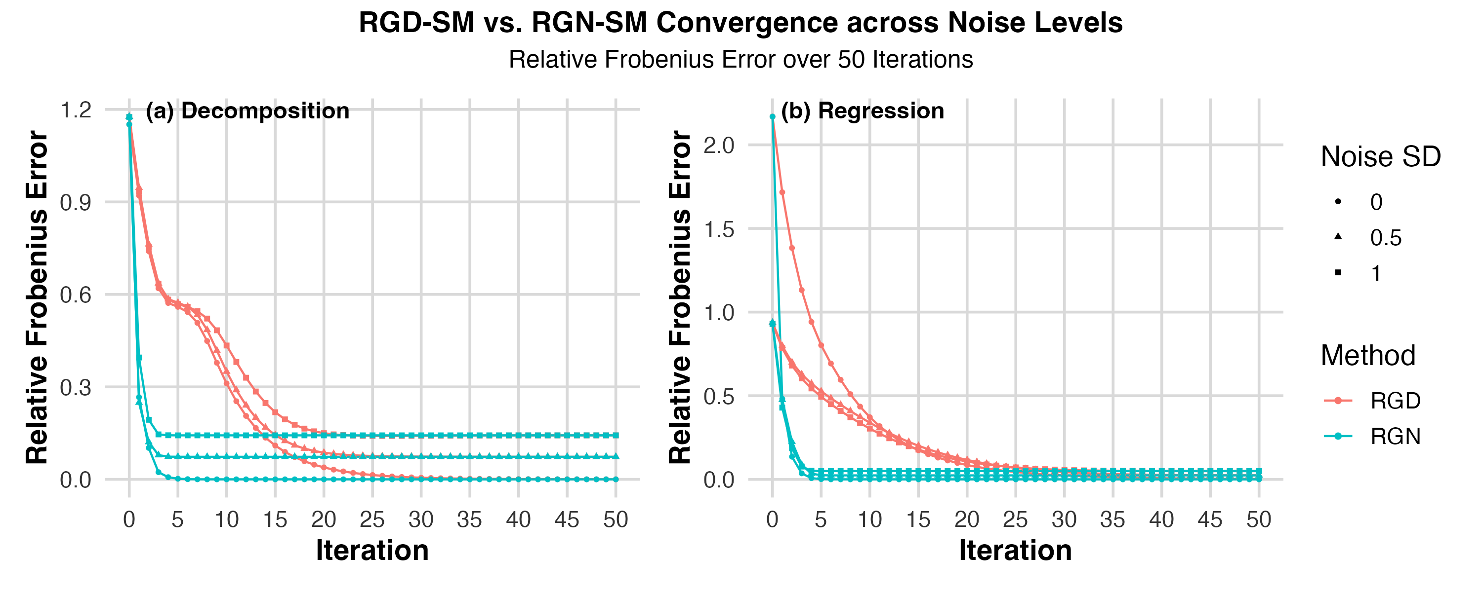
We evaluate the convergence behavior of the proposed RGD and RGN methods on two representative problems: (i) CP tensor decomposition, and (ii) scalarโ€onโ€tensor regression with a low CP rank signal tensor. In all experiments, we work with a thirdโ€order tensor of dimension $(p_{1},p_{2},p_{3})=(30,30,30)$ and a true CP rank $r=3$. The step-size $\alpha_{t}$ for RGD is fixed at 0.2. The factor vectors $\{u_{l,i}\}_{l\in[d],i\in[r]}$ are sampled independently from $\mathcal{N}(0,I_{p_{l}})$ and then normalized to unit $\ell_{2}$โ€norm, i.e. uniformly sampled from the sphere $\SS^{p_{l}-1}$. Let $\bar{p}=\max\{p_{1},p_{2},p_{3}\}$.

In the CP decomposition setting, we generate the noise tensor $\mathcal{E}$ with i.i.d $\mathcal{N}(0,1)$ entries. We simulate the signal $\{\lambda_{i}\}_{i=1}^{r}$ from $(\sqrt{d}+1)\cdot\operatorname{Unif}(\bar{p}^{3/4},2\cdot\bar{p}^{3/4})$. For regression, we draw the noise terms $\{\xi_{m}\}_{m=1}^{n}$ i.i.d from $\mathcal{N}(0,1)$ and generate i.i.d. standard Gaussian design tensors $\{\mathcal{X}_{m}\}_{m=1}^{n}$. We sample the signal weights $(\sqrt{d}+1)\cdot\operatorname{Unif}(0.5,1.5)$ and fix the sample size $n$ to be $2\bar{p}^{3/2}r$.

Convergence of Riemannian Optimization Methods.

We measure performance using the relative Frobenius error $\|\widehat{\mathcal{T}}-\mathcal{T}\|_{\mathrm{F}}/\|\mathcal{T}\|_{\mathrm{F}}$. The error metric $\max_{i\in[r]}(\|\widehat{\mathcal{T}}_{i}-\mathcal{T}_{i}\|_{\mathrm{F}}/\lambda_{i})$ used in the theoretical analysis is more sensitive to the identifiability issue across $r$ components while the relative Frobenius norm provides a stable summary. Our theoretical analysis results can be immediately extended to the error contraction of the relative Frobenius error. Figureย 1 shows that, in both scenarios, without noise, RGDโ€™s error decays linearly and RGNโ€™s decays quadratically to zero; under noise, RGD contracts linearly to its noise floor, while RGN retains a quadratic rate until it reaches its noiseโ€dependent limit. We tried several other simulation settings in which we varied the standard deviation of noise and observed a similar phenomenon.

Refer to caption
Figure 1: Convergence of RGD and RGN for (a) CP decomposition and (b) tensor regression, plotted in terms of relative Frobenius error versus iteration.

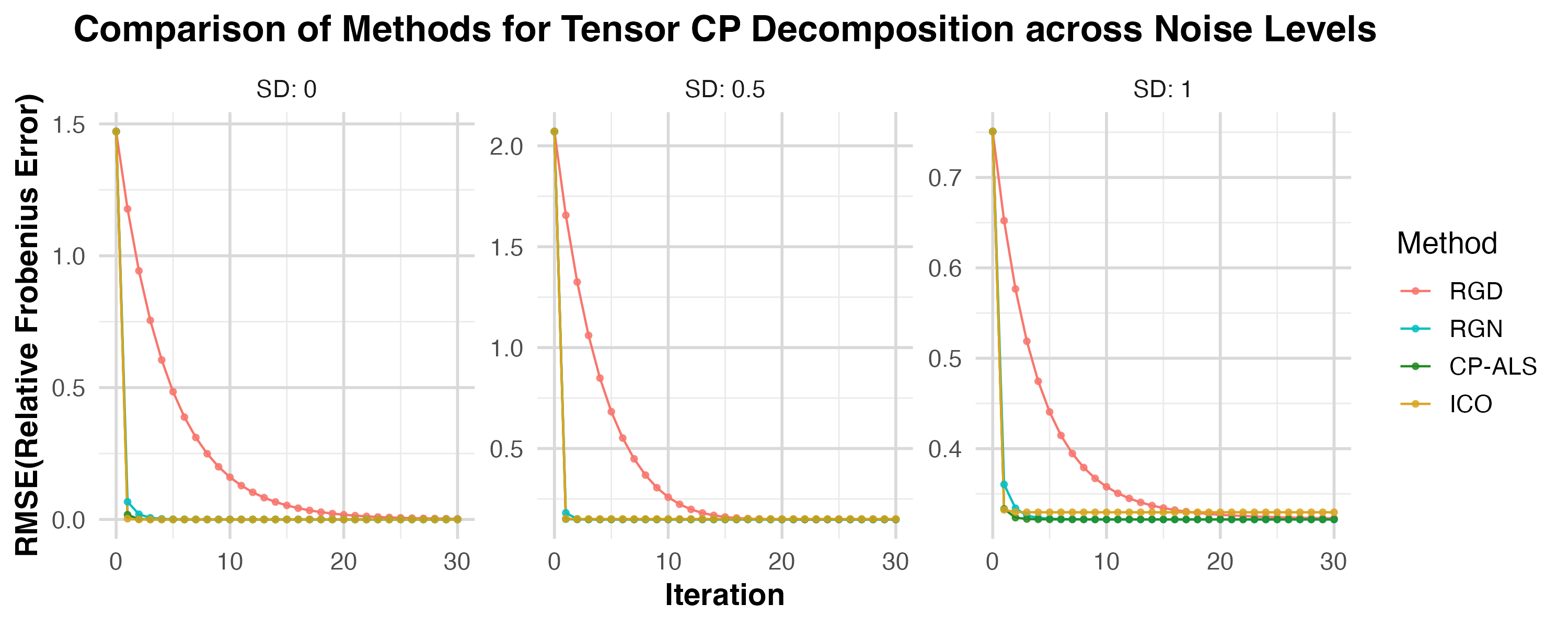
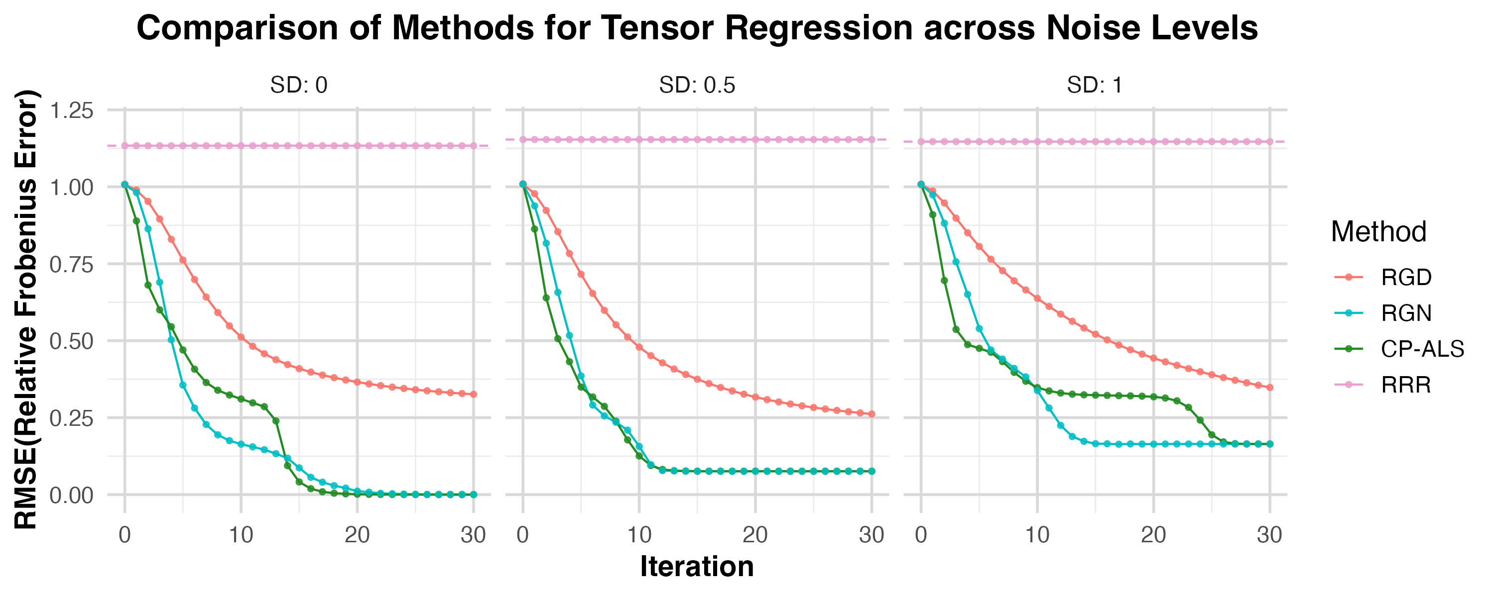
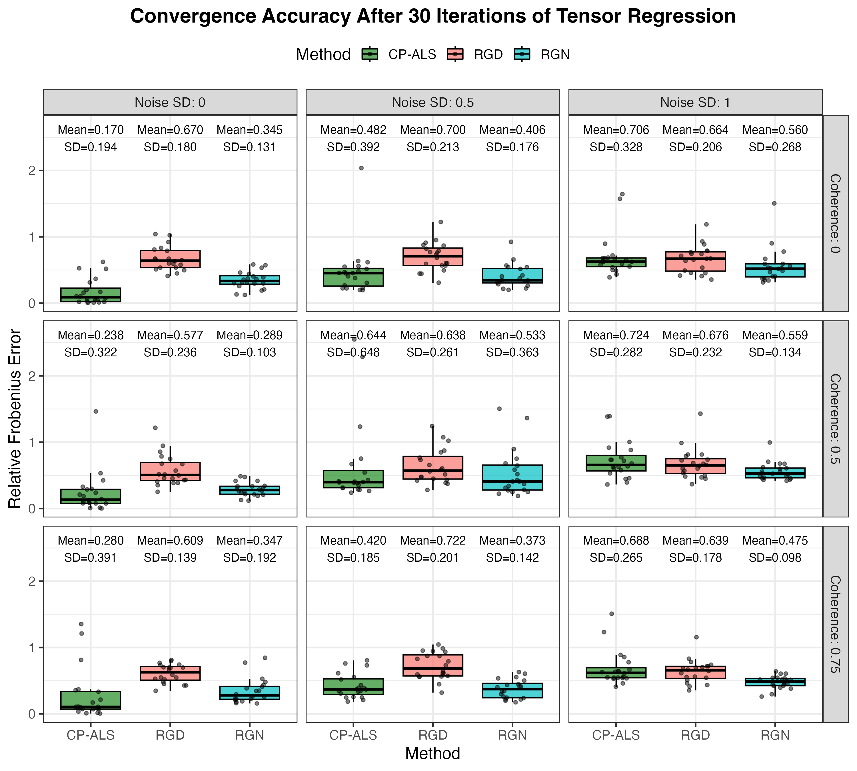
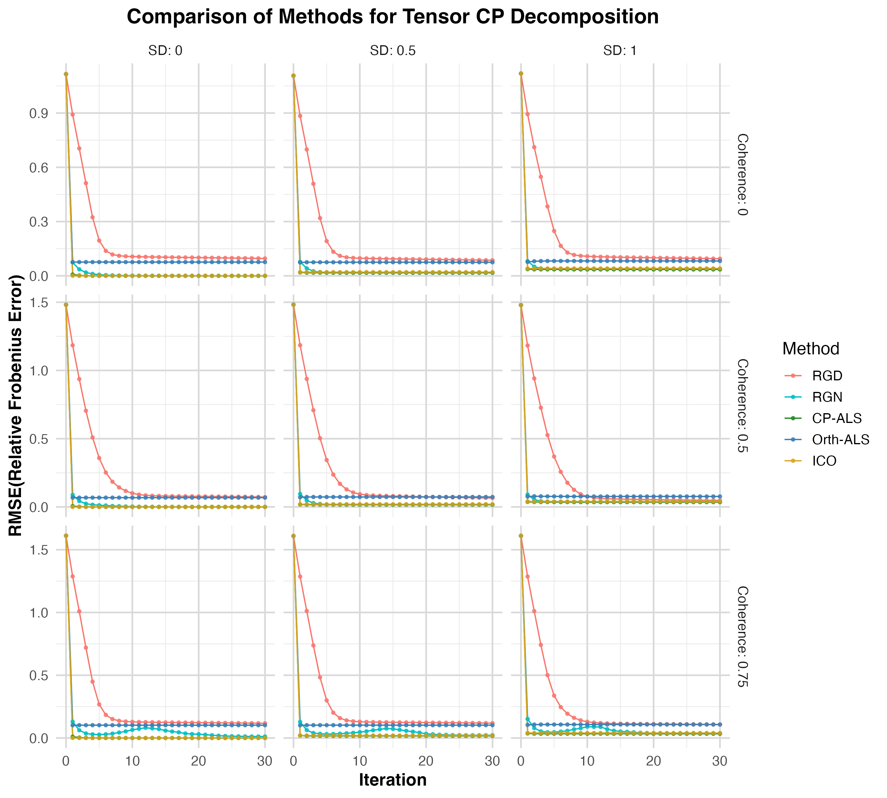
Comparison of RGD and RGN with Existing Algorithms.

In this subsection, we compare RGD and RGN with other existing algorithms, including Alternating Least Squares (CP-ALS) Kolda and Bader, (2009), Iterative Concurrent Orthogonalization (ICO) Han and Zhang, (2022) for CP decomposition, and penalized reduced rank regression (RRR) for tensor regression Lock, (2018). Since RRR is not an iterative algorithm, we plot only its final relative error. We replicate the simulation 20 times for stable results and present the square root of the mean of the relative Frobenius error. Here, we introduce coherence for factors by ensuring all columns have $\eta=0.75$ with a common reference. The implementation details are provided in the appendix. In CP decomposition (Figureย 2), RGN matches the rapid 1-2 iteration convergence of CP-ALS and ICO. In regression (Figureย 3), RGN outperforms CP-ALS and demonstrates greater robustness, while RGD converges more slowly, and RRR converges to a solution with a significantly higher estimation error. Unlike CP-ALS, which lacks theoretical guarantees, RGN combines provable local quadratic convergence with strong empirical performance and broad applicability.

Refer to caption
Figure 2: Convergence of CP tensor decomposition algorithms in terms of relative Frobenius error versus iteration: RGD-SM and RGN-SM (proposed) compared with CP-ALS Kolda and Bader, (2009) and ICO Han and Zhang, (2022).
Refer to caption
Figure 3: Convergence of CP tensor regression algorithms in terms of relative Frobenius error versus iteration: RGD-SM and RGN-SM (proposed) compared with CP-ALS Kolda and Bader, (2009) and RRR Lock, (2018).

6 Discussion and Future Extensions

In this paper, we propose a unified and provably convergent framework for both CP tensor decomposition and scalar-on-tensor regression with a CP low-rank signal tensor under additive noise. Our approach reformulates each problem as a Riemannian optimization over the Segre manifold of rank-one tensors. Extensive simulations show that our method matches the convergence speed of CP-ALS in the CP decomposition setting and slightly outperforms it in terms of final estimation error in the regression setting.

Our framework offers several practical advantages. It seamlessly handles a broad class of linear measurement operators and can be extended to CP tensor completion in future work. Moreover, because each component is updated independently on the Segre manifold, our methods allow for streaming implementations, which are ideal for large-scale or time-evolving tensor data. While we use fixed step sizes here, adaptive schemes or Riemannian momentum could further speed up convergence.

Despite these advantages, our framework has some limitations that remain open. First, our analysis assumes exact knowledge of the CP rank and does not address rank selection or mis-specification. Second, each iteration requires Riemannian retractions and tangent-space projections, which can become computationally costly in high dimensions or at large ranks. Addressing these issues is an important direction for future work.

Several challenges remain. First, our analysis presumes the CP rank is known exactly; extending the theory to handle rank selection or rank mis-specification is important. Second, each iteration involves retractions and tangent-space projections, which may become computationally intensive in ultra-high dimensions. Developing more efficient approximations or randomized updates would be a valuable direction for future research.

References

  • (1) Anandkumar, A., Ge, R., Hsu, D.ย J., Kakade, S.ย M., Telgarsky, M., etย al. (2014a). Tensor decompositions for learning latent variable models. J. Mach. Learn. Res., 15(1):2773โ€“2832.
  • (2) Anandkumar, A., Ge, R., and Janzamin, M. (2014b). Guaranteed non-orthogonal tensor decomposition via alternating rank-$1$ updates. arXiv preprint arXiv:1402.5180.
  • Bi etย al., (2021) Bi, X., Tang, X., Yuan, Y., Zhang, Y., and Qu, A. (2021). Tensors in statistics. Annual review of statistics and its application, 8(1):345โ€“368.
  • Boumal, (2023) Boumal, N. (2023). An introduction to optimization on smooth manifolds. Cambridge University Press.
  • Cai etย al., (2020) Cai, C., Poor, H.ย V., and Chen, Y. (2020). Uncertainty quantification for nonconvex tensor completion: Confidence intervals, heteroscedasticity and optimality. In International Conference on Machine Learning, pages 1271โ€“1282. PMLR.
  • Cai etย al., (2022) Cai, C., Poor, H.ย V., and Chen, Y. (2022). Uncertainty quantification for nonconvex tensor completion: Confidence intervals, heteroscedasticity and optimality. IEEE Transactions on Information Theory, 69(1):407โ€“452.
  • Carroll and Chang, (1970) Carroll, J.ย D. and Chang, J.-J. (1970). Analysis of individual differences in multidimensional scaling via an n-way generalization of โ€œeckart-youngโ€ decomposition. Psychometrika, 35(3):283โ€“319.
  • Comon etย al., (2009) Comon, P., Luciani, X., and Deย Almeida, A.ย L. (2009). Tensor decompositions, alternating least squares and other tales. Journal of Chemometrics: A Journal of the Chemometrics Society, 23(7-8):393โ€“405.
  • Deย Lathauwer etย al., (2000) Deย Lathauwer, L., Deย Moor, B., and Vandewalle, J. (2000). A multilinear singular value decomposition. SIAM journal on Matrix Analysis and Applications, 21(4):1253โ€“1278.
  • Frolov and Oseledets, (2017) Frolov, E. and Oseledets, I. (2017). Tensor methods and recommender systems. Wiley Interdisciplinary Reviews: Data Mining and Knowledge Discovery, 7(3):e1201.
  • Hackbusch, (2012) Hackbusch, W. (2012). Tensor spaces and numerical tensor calculus, volumeย 42. Springer.
  • Han etย al., (2022) Han, R., Willett, R., and Zhang, A.ย R. (2022). An optimal statistical and computational framework for generalized tensor estimation. The Annals of Statistics, 50(1):1โ€“29.
  • Han and Zhang, (2022) Han, Y. and Zhang, C.-H. (2022). Tensor principal component analysis in high dimensional cp models. IEEE Transactions on Information Theory, 69(2):1147โ€“1167.
  • Harshman etย al., (1970) Harshman, R.ย A. etย al. (1970). Foundations of the parafac procedure: Models and conditions for an โ€œexplanatoryโ€ multi-modal factor analysis. UCLA working papers in phonetics, 16(1):84.
  • Jacobsson etย al., (2024) Jacobsson, S., Swijsen, L., Vanย der Veken, J., and Vannieuwenhoven, N. (2024). Warped geometries of segre-veronese manifolds. arXiv preprint arXiv:2410.00664.
  • Kolda and Bader, (2009) Kolda, T.ย G. and Bader, B.ย W. (2009). Tensor decompositions and applications. SIAM review, 51(3):455โ€“500.
  • Kressner etย al., (2014) Kressner, D., Steinlechner, M., and Vandereycken, B. (2014). Low-rank tensor completion by riemannian optimization. BIT Numerical Mathematics, 54:447โ€“468.
  • Kruskal, (1977) Kruskal, J.ย B. (1977). Three-way arrays: rank and uniqueness of trilinear decompositions, with application to arithmetic complexity and statistics. Linear algebra and its applications, 18(2):95โ€“138.
  • Landsberg, (2011) Landsberg, J.ย M. (2011). Tensors: geometry and applications, volume 128. American Mathematical Soc.
  • Lock, (2018) Lock, E.ย F. (2018). Tensor-on-tensor regression. Journal of Computational and Graphical Statistics, 27(3):638โ€“647.
  • Luo and Zhang, (2023) Luo, Y. and Zhang, A.ย R. (2023). Low-rank tensor estimation via riemannian gauss-newton: Statistical optimality and second-order convergence. Journal of Machine Learning Research, 24(381):1โ€“48.
  • Luo and Zhang, (2024) Luo, Y. and Zhang, A.ย R. (2024). Tensor-on-tensor regression: Riemannian optimization, over-parameterization, statistical-computational gap and their interplay. The Annals of Statistics, 52(6):2583โ€“2612.
  • Montanari and Richard, (2014) Montanari, A. and Richard, E. (2014). A statistical model for tensor pca. Advances in neural information processing systems, 27.
  • Rauhut etย al., (2017) Rauhut, H., Schneider, R., and Stojanac, ลฝ. (2017). Low rank tensor recovery via iterative hard thresholding. Linear Algebra and its Applications, 523:220โ€“262.
  • Sharan and Valiant, (2017) Sharan, V. and Valiant, G. (2017). Orthogonalized als: A theoretically principled tensor decomposition algorithm for practical use. In International Conference on Machine Learning, pages 3095โ€“3104. PMLR.
  • Sun etย al., (2017) Sun, W.ย W., Lu, J., Liu, H., and Cheng, G. (2017). Provable sparse tensor decomposition. Journal of the Royal Statistical Society Series B: Statistical Methodology, 79(3):899โ€“916.
  • Swijsen etย al., (2022) Swijsen, L., Vanย der Veken, J., and Vannieuwenhoven, N. (2022). Tensor completion using geodesics on segre manifolds. Numerical Linear Algebra with Applications, 29(6):e2446.
  • Tang and Li, (2023) Tang, X. and Li, L. (2023). Multivariate temporal point process regression. Journal of the American Statistical Association, 118(542):830โ€“845.
  • Vannieuwenhoven etย al., (2012) Vannieuwenhoven, N., Vandebril, R., and Meerbergen, K. (2012). A new truncation strategy for the higher-order singular value decomposition. SIAM Journal on Scientific Computing, 34(2):A1027โ€“A1052.
  • Vershynin, (2018) Vershynin, R. (2018). High-dimensional probability: An introduction with applications in data science, volumeย 47. Cambridge university press.
  • Wang and Lu, (2017) Wang, P.-A. and Lu, C.-J. (2017). Tensor decomposition via simultaneous power iteration. In International Conference on Machine Learning, pages 3665โ€“3673. PMLR.
  • Zhang etย al., (2020) Zhang, A.ย R., Luo, Y., Raskutti, G., and Yuan, M. (2020). Islet: Fast and optimal low-rank tensor regression via importance sketching. SIAM journal on mathematics of data science, 2(2):444โ€“479.
  • Zhang and Golub, (2001) Zhang, T. and Golub, G.ย H. (2001). Rank-one approximation to high order tensors. SIAM Journal on Matrix Analysis and Applications, 23(2):534โ€“550.

Appendices

Appendix A Notation

Throughout this paper, we use the following notation and conventions.

We use boldface uppercase calligraphic letters (e.g. $\mathcal{T},\mathcal{X}$) for tensors, uppercase letters (e.g. $A,U$) for matrices, and lowercase letters (e.g. $u,v$) for vectors or scalars. For any positive integer $m$, let $[m]={1,2,\dots,m}$. We consider order-$d$ tensors with mode dimensions $p_{1},p_{2},\dots,p_{d}$, so that $\mathcal{T}\in\mathbb{R}^{p_{1}\times\cdots\times p_{d}}$ contains $p^{*}=\prod_{l=1}^{d}p_{l}$ total entries. The CP rank is denoted by $r$, and the sample size in regression contexts is denoted by $n$.

The vectorization of a tensor $\mathcal{T}$ is denoted by $\operatorname{vec}(\mathcal{T})$. The mode-$k$ unfolding (matricization) is $\hbox{\rm mat}_{k}(\mathcal{T})\in\mathbb{R}^{p_{k}\times(p/p_{k})}$. The outer (tensor) product is written $\otimes$. The multilinear (Tucker) product of $\mathcal{T}$ with matrices $U_{k}\in\mathbb{R}^{q_{k}\times p_{k}}$ is $\mathcal{T}\times_{1}U_{1}\times_{2}\cdots\times_{d}U_{d}$. The $k$-mode product with $U$ alone is $\mathcal{T}\times_{k}U$. The tensor inner product is $\langle\mathcal{A},\mathcal{B}\rangle=\sum_{i_{1},\ldots,i_{d}}A_{i_{1}\dots i_{d}}B_{i_{1}\dots i_{d}}$. The induced Frobenius norm is $\|\mathcal{A}\|_{\mathrm{F}}=\sqrt{\langle\mathcal{A},\mathcal{A}\rangle}$. For matrices and vectors, $\|\cdot\|_{\mathrm{F}}$ and $\|\cdot\|$ denote the Frobenius and spectral (or Euclidean) norms, respectively.

Let $\SS^{p-1}$ denote the unit sphere in $\mathbb{R}^{p}$. Define the Stiefel manifold $\mathbb{O}^{p,r}={U\in\mathbb{R}^{p\times r}:U^{\top}U=I_{r}}$ as the set of $p\times r$ orthonormal matrices. For any $U\in\mathbb{O}^{p,r}$, the orthogonal projection onto its column space is $\mathcal{P}_{U}=UU^{\top}$.

In particular, for a unit vector $u\in\mathbb{R}^{p}$, define the projector onto its span as $P_{u}=uu^{\top}$ and its orthogonal complement as $P_{u}^{\perp}=I_{p}-uu^{\top}$. We use $\mathbb{R}^{+}$ to denote the set of positive real numbers. For rank-one tensors, these projections are applied in a mode-wise manner. The set of nonzero rank-one tensors of the form $u_{1}\otimes\cdots\otimes u_{d}$, where each $u_{k}\in\mathbb{R}^{p_{k}}\setminus\{0\}$, forms the Segre manifold. Its geometric structure, including tangent spaces, Riemannian gradients, and retraction maps, is further discussed in Sectionย 3.2.

Appendix B Additional Simulation Results

In well-conditioned regimes, characterized by low tensor condition numbers, high signal-to-noise ratios (SNR), and moderate incoherence, Alternating Least Squares (ALS) remains the de facto gold standard for CP decomposition. In such favorable settings, our proposed Riemannian Gradient Descent (RGD) and Riemannian Gaussโ€“Newton (RGN) algorithms offer theoretically grounded alternatives to ALS. However, when these conditions are violated, ALS often struggles to converge reliably (Sharan and Valiant,, 2017). To evaluate algorithmic stability and accuracy in such challenging settings, we extend the numerical experiments presented in the main text and empirically demonstrate the advantages of the proposed Riemannian optimization methods in the ill-posed regime.

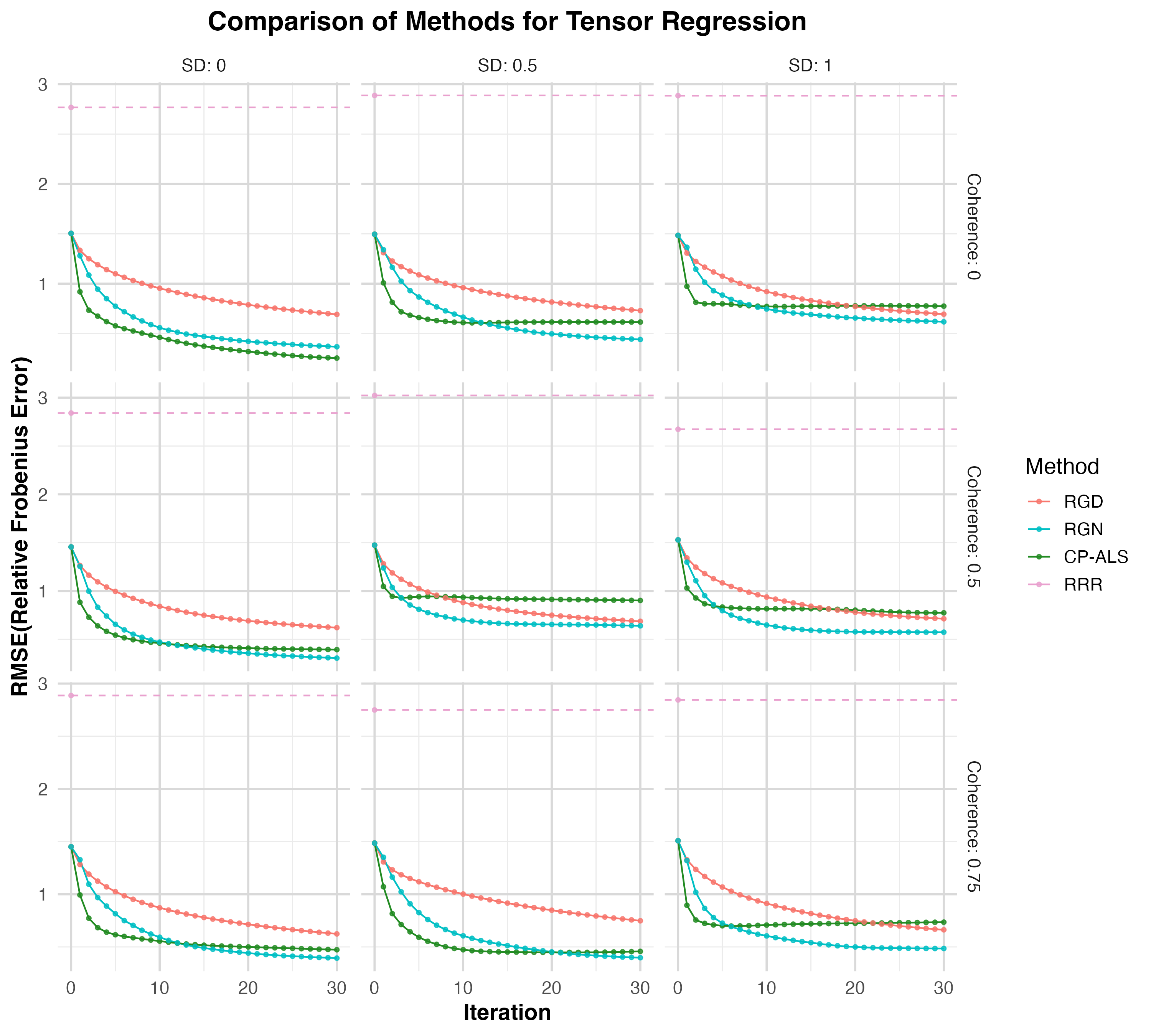
Results for Tensor Regression.

For tensor regression, we use the same tensor dimensions and rank: $(p_{1},p_{2},p_{3})=(20,20,20)$ and $r=3$. The noise variance of the design tensor is fixed at $\sigma^{2}=1$, and the sample size is set to $n=2p^{3/2}r$. The factor weights are defined as $\lambda_{i}=2\kappa^{(i-2)/2}$ for $i=1,2,3$, with the condition number $\kappa=10$. We vary the standard deviation of the additive noise over $\{0,0.5,1\}$ and the coherence parameter over $\{0,0.5,0.75\}$. Figureย 4 illustrates the iterationโ€wise convergence of the relative Frobenius reconstruction error over 30 iterations, while Figureย 5 summarizes the error distributions after 30 iterations.

Refer to caption
Figure 4: Convergence of the relative Frobenius reconstruction error over 30 iterations for various noise scales and coherence numbers. Curves are averaged over all 20 independent replicates.
Refer to caption
Figure 5: Error distributions after 30 iterations for various noise scales and coherence numbers. Boxes summarize the spread over 20 replicates.

Results for CP Decomposition.

We fix the tensor dimensions to $(p_{1},p_{2},p_{3})=(20,20,20)$ and set the CP rank to $r=3$. The factor weights are defined as $\lambda_{i}=2\kappa^{(i-1)/2}p^{3/4}r^{1/2}$ for $i=1,2,3$, with the condition number $\kappa=10$. We vary the noise standard deviation and coherence as before. Figureย 6 shows the convergence trajectory of the relative Frobenius reconstruction error over 30 iterations. Figureย 7 presents the distribution of reconstruction errors after 30 iterations.

Refer to caption
Figure 6: Convergence of the relative Frobenius reconstruction error over 30 iterations for various noise scales and coherence numbers. Curves are averaged over all 20 independent replicates.
Refer to caption
Figure 7: Error distributions after 30 iterations for various noise scales and coherence numbers. Boxes summarize the spread over 20 replicates.

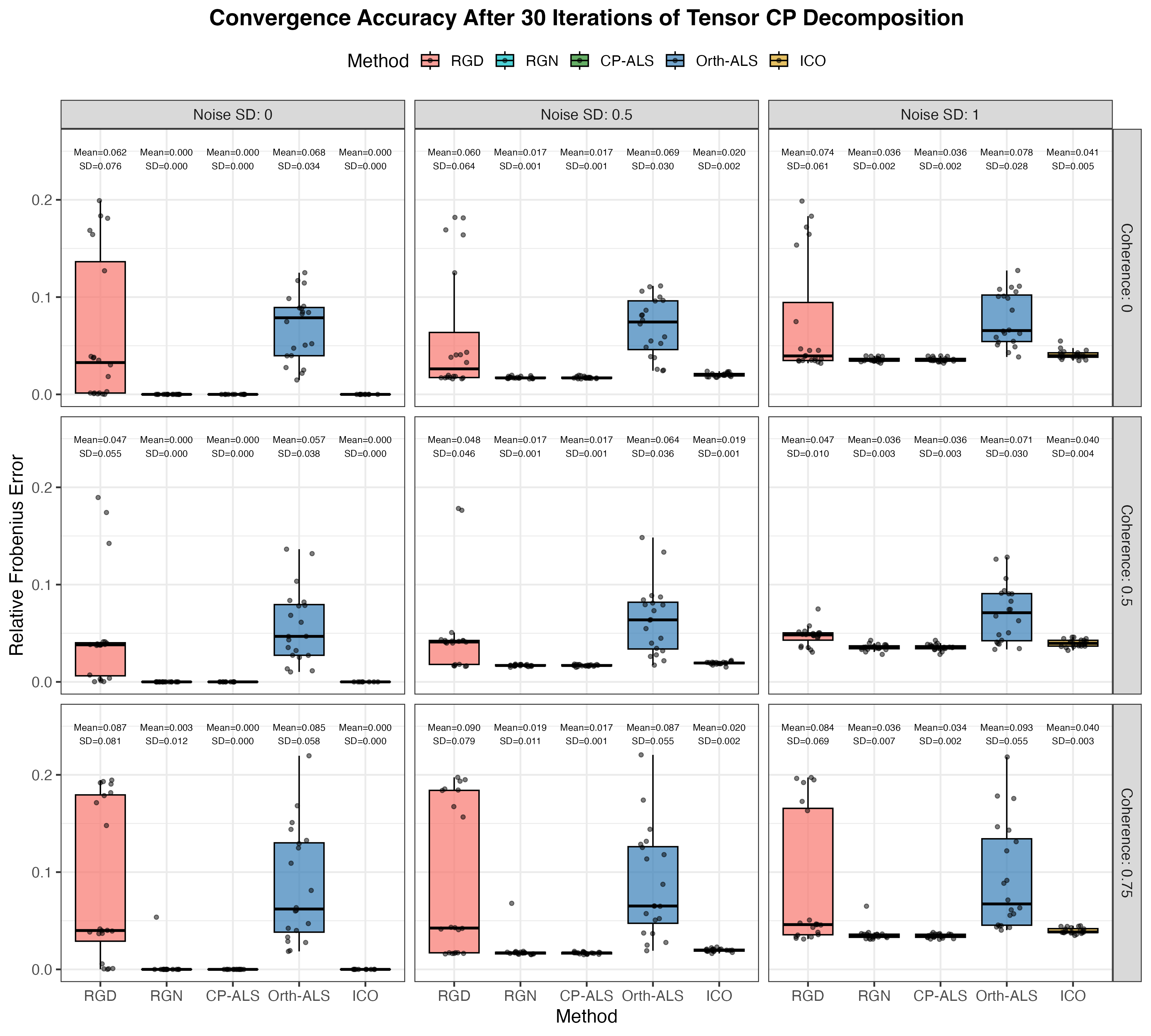
Overall, under the setting of tensor regression, the results show that the proposed RGN algorithm consistently outperforms CP-ALS in terms of reconstruction accuracy, particularly at increased coherence and noise levels. Under the setting of tensor CP decomposition, our RGN method outperforms Orthogonalized-ALS (Sharan and Valiant,, 2017) and ICO (Han and Zhang,, 2022), and attains quite similar performance compared with ALS.

Appendix C Additional Details on Algorithms

In this section, we provide additional details on the algorithmic implementation and data generation for simulation in the main text.

Incoherence condition

To explore scenarios with non-orthogonal factors, we generate factor matrices whose columns achieve a prescribed level of pairwise coherence. Specifically, for a given coherence parameter $\rho\in[0,1)$ and target rank $R$, we first construct the $R\times R$ Gram matrix

$$G_{ij}=\rho^{|i-j|},\quad i,j\in[R],$$

which corresponds to an autoregressive correlation structure of order one (AR(1)). We then compute the Cholesky factor $C$ of $G$ and embed it into $\mathbb{R}^{p}$ by stacking $R$ identity rows on top of $(p-R)$ zero rows, forming an initial matrix $Q_{0}\in\mathbb{R}^{p\times R}$. Multiplying $Q_{0}$ with $C$ yields vectors with the desired correlation pattern, and each column is normalized to unit length.

Finally, to avoid artificial alignment with the coordinate axes, we apply a random orthogonal rotation by multiplying with a Haar-distributed orthogonal matrix. The resulting factor matrix thus has columns with controlled coherence while preserving rotational invariance in $\mathbb{R}^{p}$. By varying $\rho$, we tune the similarity (โ€œcoherenceโ€) between the factors: $\rho=0$ corresponds to orthogonal columns, whereas $\rho$ close to $1$ yields highly coherent columns.

Initialization

For tensor regression, we employ the Composite Principal Component Analysis (CPCA) method proposed by Han and Zhang, (2022) as a warm-start initialization. CPCA generates reliable initial estimates of the CP basis vectors by performing a specialized unfolding-refolding procedure followed by spectral decomposition. It has been shown that CPCA consistently outperforms the classical higher-order singular value decomposition (T-HOSVD) initialization (Deย Lathauwer etย al.,, 2000) in terms of the quality of the final solution.

In contrast, for tensor CP decomposition, we adopt random initialization. This choice aligns with the current theoretical framework, which establishes convergence guarantees under random initialization settings (Sharan and Valiant,, 2017).

C.1 Implementation details

We provide implementation details for the algorithms evaluated in our experiments.

The Orthogonalized ALS (Orth-ALS) algorithm for tensor CP decomposition is adapted from the publicly available MATLAB implementation provided by Sharan and Valiant, (2017). We adopt the version of Orth-ALS that performs orthogonalization before every ALS step. The CP-ALS algorithm for tensor CP decomposition is modified from the CP function in the rTensor R package. We extend the original implementation by incorporating custom initialization routines and error tracking at each iteration.

For tensor regression, the Reduced-Rank Regression (RRR) method is directly accessed via the rrr() function in the R package MultiwayRegression. The CP-ALS regression method is implemented by adapting the CP-ALS algorithm to the tensor regression setting. In each iteration, the algorithm solves a least squares problem to update each mode factor matrix while keeping the others fixed, similar in spirit to alternating least squares for CP decomposition, but applied to the regression loss.

All simulations and benchmarking experiments are performed in R (version 4.4.3) on a MacBook Air (2022) equipped with an Apple M2 chip and 8GB of RAM.

C.2 Tensor CP decomposition

Initialization for the CP decomposition

Here, we use a composite PCA (CPCA, Algorithm 4 in Han and Zhang, (2022)) as a warm-start initialization for tensor CP decomposition. Let $p^{*}=\prod_{l\in[d]}p_{l}$.

Algorithm 3 Composite PCA (CPCA) for general $N$-th order tensors Han and Zhang, (2022)

Input: Noisy tensor $\mathcal{Y}$, CP rank $r$, subset $S\subset[d]$

1:โ€‚if $S=\varnothing$ then
2:โ€ƒโ€‚Pick $S$ to maximize $\min(p_{S},p^{*}/p_{S})$ where $p_{S}=\prod_{l\in S}p_{k}$ and $p=\prod_{l\in[d]}p_{l}$
3:โ€‚end if
4:โ€‚Unfold $T$ into a $p_{S}\times(p/p_{S})$ matrix $\hbox{\rm mat}_{S}(\mathcal{T})$
5:โ€‚Compute topโ€‘rr SVD:
$$\hbox{\rm mat}_{S}(\mathcal{T})=\sum_{j=1}^{r}\hat{\lambda}_{j}^{\mathrm{cpca}}\,\hat{u}_{j}\,\hat{v}_{j}^{\top}$$
6:โ€‚for $i=1$ to $r$ do
7:โ€ƒโ€‚for $k\in S$ do
8:$\widehat{u}_{l,i}^{\mathrm{cpca}}\leftarrow$ leading left singular vector of $\hbox{\rm mat}_{l}(\widehat{u}_{i})$
9:โ€ƒโ€‚end for
10:โ€‚end for
11:โ€‚return $\{\widehat{u}_{l,i}^{\mathrm{cpca}},\,\hat{\lambda}_{i}^{\mathrm{cpca}}\}_{l\in[d],i\in[r]}$

Riemann Gradient Descent for Tensor Decomposition

Algorithm 4 Riemannian Gradient Descent for CP Tensor Decomposition

Input: Noisy tensor $\mathcal{Y}$, input CP rank $r$, step size $\alpha_{t}$, and $r$ rank-one tensor initialization $\left\{\mathcal{T}_{i}^{(0)}\right\}_{i=1}^{r}$.

1:โ€‚for $t=0,1,\dots,t_{\max}-1$ do
2:โ€ƒโ€‚for $i=1,\dots,r$ do
3:โ€ƒโ€ƒโ€‚(RGD Update) Compute
$$\mathcal{T}_{i}^{(t+1)}=\mathcal{R}_{\mathcal{T}_{i}^{(t)}}\left(\mathcal{T}_{i}^{(t)}-\alpha_{t}\mathcal{P}_{\mathbb{T}_{i}^{(t)}}\left(\sum_{i=1}^{r}\left(\mathcal{T}_{i}^{(t)}\right)-\mathcal{Y}\right)\right),$$
where $\alpha_{t}$ is the step size, $\mathcal{P}_{\mathbb{T}_{i}^{(t)}}\left(\cdot\right)$ denotes the projection onto the tangent space $\mathbb{T}_{i}^{(t)}$ of Segre manifold at $\mathcal{T}_{i}^{(t)}$, which is given by (3), and $\mathcal{R}_{\mathcal{T}_{i}^{(t)}}$ is a retraction given by T-HOSVD.
4:โ€ƒโ€‚end for
5:โ€‚end for

Output: $\left\{\mathcal{T}_{i}^{(t_{\max})}\right\}_{i=1}^{r}$.

Let $U_{l}=\left[u_{l,1},u_{l,2},\cdots,u_{l,r}\right]\in\mathbb{R}^{p_{l}\times r}$ for $l\in[d]$. Then we use $\max_{l\in[d]}\max_{i\in[r]}\left\|\widehat{u}_{l,i}\widehat{u}_{l,i}^{\top}-u_{l,i}u_{l,i}^{\top}\right\|$ as the error metric to check the convergence of the error contraction with respect to the number of iterations. Throughout the numerical experiments for RGD in this paper, we set a constant step size $\alpha_{t}\equiv 0.2$.

Riemann Gauss-Newton for Tensor Decomposition

For tensor decomposition, Riemann-Gauss-Newton is equivalent to the case where the step size $\alpha_{t}\equiv 1$.

Algorithm 5 Riemannian Gauss-Newton for CP Tensor Decomposition

Input: Noisy tensor $\mathcal{Y}$, input CP rank $r$, and $r$ rank-one tensor initialization $\left\{\mathcal{T}_{i}^{(0)}\right\}_{i=1}^{r}$.

1:โ€‚for $t=0,1,\dots,t_{\max}-1$ do
2:โ€ƒโ€‚for $i=1,\dots,r$ do
3:โ€ƒโ€ƒโ€‚(RGN Update)
$$\mathcal{T}_{i}^{(t+1)}=\mathcal{R}_{\mathcal{T}_{i}^{(t)}}\left(\mathcal{T}_{i}^{(t)}-\mathcal{P}_{\mathbb{T}_{i}^{(t)}}\left(\sum_{i=1}^{r}\mathcal{T}_{i}^{(t)}-\mathcal{Y}\right)\right),$$
where $\mathcal{P}_{\mathbb{T}_{i}^{(t)}}\left(\cdot\right)$ denotes the projection onto the tangent space $\mathbb{T}_{i}^{(t)}$ of Segre manifold at $\mathcal{T}_{i}^{(t)}$, which is given by (3), and $\mathcal{R}_{\mathcal{T}_{i}^{(t)}}$ is a retraction given by T-HOSVD.
4:โ€ƒโ€‚end for
5:โ€‚end for

Output: $\left\{\mathcal{T}_{i}^{(t_{\max})}\right\}_{i=1}^{r}$.

C.3 Tensor Regression

Initialization for tensor regression

To estimate the low-rank tensor coefficient in a regression setting, we adopt an initialization strategy based on the adjoint operator of the linear map $\mathcal{A}$ induced by the covariates $\left\{\mathcal{X}_{m}\right\}_{m=1}^{n}$. Specifically, the adjoint estimator is given by:

$$\mathcal{A}^{*}\left(\mathcal{Y}\right)=\frac{1}{n\sigma^{2}}\sum_{m=1}^{n}y_{m}\mathcal{X}_{m}$$

which provides a consistent but potentially noisy estimate of the true coefficient tensor under suitable conditions on the design tensors $\mathcal{X}_{m}$ Han etย al., (2022); Zhang etย al., (2020). Following this, we compute a rank-$r$ approximation of $\mathcal{A}^{*}(\mathcal{Y})$ using CPCA as proposed by Han and Zhang, (2022). The result yields both singular values and orthonormal mode matrices $\left\{U_{l}\right\}_{l\in[d]}$ for initialization. In the implementation of our algorithm, we first rescale the observed data $\frac{1}{\sqrt{n\sigma}}\{\mathcal{X}_{m},y_{m}\}_{m=1}^{n}$.

Algorithm 6 Initialization of Lowโ€rank Tensor Regression

Input: (Rescaled) Observation $\{\mathcal{X}_{m},y_{m}\}_{m=1}^{n}$, input CP rank $r$

1:โ€‚Compute
$$\widetilde{\mathcal{X}}=\sum_{m=1}^{n}y_{m}\,\mathcal{X}_{m}=\mathcal{A}^{*}\left(\mathcal{Y}\right)$$
2:โ€‚Compute CPCA of $\widetilde{\mathcal{X}}$: $\left(\Lambda,\,U_{1},U_{2},\cdots,U_{d}\right)\leftarrow\texttt{CPCA}(\tilde{\mathcal{X}})$ where CPCA is defined in Han and Zhang, (2022). Here, $\Lambda=\left(\lambda_{1},\lambda_{2},\cdots,\lambda_{r}\right)\in\mathbb{R}^{r}$ and $U_{l}=\left(u_{l,1},u_{l,2},\cdots,u_{l,r}\right)\in\mathbb{R}^{p_{l}\times r}$ for any $l\in[d]$.
3:โ€‚return $\left(\Lambda,\,U_{1},U_{2},\cdots,U_{d}\right)$

Riemann Gradient Descent for Tensor regression

The RGD procedure updates each rank-one tensor component $\mathcal{T}_{i}^{(t)}=\lambda_{i}u_{1,i}^{(t)}\otimes\cdots\otimes u_{d,i}^{(t)}$ iteratively via tangent space projections and retractions.

Algorithm 7 Riemannian Gradient Descent for CP Tensor Regression

Input: (Rescaled) Observation $\{\mathcal{X}_{m},y_{m}\}_{m=1}^{n}$, input CP rank $r$, step size $\alpha_{t}$, and $r$ rank-one tensor initialization $\left\{\mathcal{T}_{i}^{(0)}\right\}_{i=1}^{r}$.

1:โ€‚for $t=0,1,\dots,t_{\max}-1$ do
2:โ€ƒโ€‚for $i=1,\dots,r$ do
3:โ€ƒโ€ƒโ€‚(RGD Update) Compute
$$\mathcal{T}_{i}^{(t+1)}=\mathcal{R}_{\mathcal{T}_{i}^{(t)}}\left(\mathcal{T}_{i}^{(t)}-\alpha_{t}\mathcal{P}_{\mathbb{T}_{i}^{(t)}}\left(\sum_{i=1}^{r}\sum_{m=1}^{n}\left\langle\mathcal{X}_{m},\mathcal{T}_{i}^{(t)}\right\rangle\mathcal{X}_{m}-\sum_{m=1}^{n}y_{m}\mathcal{X}_{m}\right)\right),$$
where $\alpha_{t}$ is the step size, $\mathcal{P}_{\mathbb{T}_{i}^{(t)}}\left(\cdot\right)$ denotes the projection onto the tangent space $\mathbb{T}_{i}^{(t)}$ of Segre manifold at $\mathcal{T}_{i}^{(t)}$, and $\mathcal{R}_{\mathcal{T}_{i}^{(t)}}$ is a retraction given by T-HOSVD.
4:โ€ƒโ€‚end for
5:โ€‚end for

Output: $\left\{\mathcal{T}_{i}^{(t_{\max})}\right\}_{i=1}^{r}$.

Riemann Gauss-Newton Update for Tensor regression

Algorithm 8 Riemannian Gauss-Newton for CP Tensor Regression

Input: (Rescaled) Observation $\{\mathcal{X}_{m},y_{m}\}_{m=1}^{n}$, input CP rank $r$, and $r$ rank-one tensor initialization $\left\{\mathcal{T}_{i}^{(0)}\right\}_{i=1}^{r}$.

1:โ€‚for $t=0,1,\dots,t_{\max}-1$ do
2:โ€ƒโ€‚for $i=1,\dots,r$ do
3:โ€ƒโ€ƒโ€‚
4:โ€ƒโ€ƒโ€‚(RGN Update)
$\displaystyle\mathcal{T}_{i}^{(t+1)}=$ โ„›๐’ฏi(t)โ€‹((๐’ซ๐•‹i(t)โ€‹๐’œโˆ—โ€‹๐’œโ€‹๐’ซ๐•‹i(t))+โ€‹๐’ซ๐•‹i(t)โ€‹๐’œโˆ—โ€‹(๐’ดโˆ’๐’œโ€‹(โˆ‘j=1,jโ‰ ir๐’ฏj(t)))),\displaystyle\mathcal{R}_{\mathcal{T}_{i}^{(t)}}\left(\left(\mathcal{P}_{\mathbb{T}_{i}^{(t)}}\mathcal{A}^{*}\mathcal{A}\mathcal{P}_{\mathbb{T}_{i}^{(t)}}\right)^{+}\mathcal{P}_{\mathbb{T}_{i}^{(t)}}\mathcal{A}^{*}\left(\mathcal{Y}-\mathcal{A}\left(\sum_{j=1,j\neq i}^{r}\mathcal{T}_{j}^{(t)}\right)\right)\right),
$\displaystyle=$ โ„›๐’ฏi(t)โ€‹((A~(t),โˆ—โ€‹A~(t))+โ€‹A~(t),โˆ—โ€‹(๐’ดโˆ’๐’œโ€‹(โˆ‘j=1,jโ‰ ir๐’ฏj(t))))\displaystyle\mathcal{R}_{\mathcal{T}_{i}^{(t)}}\left(\left(\widetilde{A}^{(t),*}\widetilde{A}^{(t)}\right)^{+}\widetilde{A}^{(t),*}\left(\mathcal{Y}-\mathcal{A}\left(\sum_{j=1,j\neq i}^{r}\mathcal{T}_{j}^{(t)}\right)\right)\right)
where $+$ denotes the Moore-Penrose pseudo inverse, $\left[\mathcal{A}\left(\mathcal{T}\right)\right]_{m}=\left\langle\mathcal{X}_{m},\mathcal{T}\right\rangle$, $\mathcal{A}^{*}\left(\mathcal{Y}\right)=\sum_{m=1}^{n}\mathcal{Y}_{m}\mathcal{X}_{m}$, $\left[\widetilde{\mathcal{A}}\left(\mathcal{T}\right)\right]_{m}=\left\langle\mathcal{P}_{\mathbb{T}_{i}^{(t)}}\left(\mathcal{X}_{m}\right),\mathcal{T}\right\rangle$ for any $m=1,2\cdots,n$ while $\widetilde{\mathcal{A}}^{(t),*}\left(\mathcal{Y}\right)=\sum_{m=1}^{n}\mathcal{Y}_{m}\mathcal{P}_{\mathbb{T}_{i}^{(t)}}\left(\mathcal{X}_{m}\right)$, $\mathcal{P}_{\mathbb{T}_{i}^{(t)}}\left(\cdot\right):\mathbb{R}^{p_{1}\times p_{2}\times\cdots\times p_{d}}\rightarrow\mathbb{R}^{p_{1}\times p_{2}\times\cdots\times p_{d}}$ denotes the projection onto the tangent space $\mathbb{T}_{i}^{(t)}$ of Segre manifold at $\mathcal{T}_{i}^{(t)}$ is given by (3), and $\mathcal{R}_{\mathcal{T}_{i}^{(t)}}$ is a retraction given by T-HOSVD.
5:โ€ƒโ€‚end for
6:โ€‚end for

Output: $\left\{\mathcal{T}_{i}^{(t_{\max})}\right\}_{i=1}^{r}$.

At each iteration, the $i$-th component is updated by solving a least-squares problem restricted to the tangent space $\mathbb{T}_{i}^{(t)}$ and subsequently retracting back onto the Segre manifold. Concretely, we first compute

๐’ฏi(t+0.5)=argโกmin๐’ฏiโˆˆ๐•‹i(t)โก12โ€‹โ€–๐’ดโˆ’๐’œโ€‹(๐’ฏi+โˆ‘jโ‰ ir๐’ฏj(t))โ€–F2\mathcal{T}_{i}^{(t+0.5)}=\arg\min_{\mathcal{T}_{i}\in\mathbb{T}_{i}^{(t)}}\frac{1}{2}\left\|\mathbf{\mathcal{Y}}-\mathcal{A}\left(\mathcal{T}_{i}+\sum_{j\neq i}^{r}\mathcal{T}_{j}^{(t)}\right)\right\|_{\mathrm{F}}^{2}

and then retract:

$$\mathcal{T}_{i}^{(t+1)}=\mathcal{R}_{\mathcal{T}_{i}^{(t)}}\left(\mathcal{T}_{i}^{(t+0.5)}\right).$$

This update can be interpreted as solving a linear regression problem using a design matrix composed of the projected tensors $\mathcal{P}_{\mathbb{T}_{i}^{(t)}}(\mathcal{X}_{m})$. The associated normal equation takes the form:

$$\left(\hbox{\rm vec}\left(\mathcal{P}_{\mathbb{T}_{i}^{(t)}}\mathcal{X}\right)^{\top}\hbox{\rm vec}\left(\mathcal{P}_{\mathbb{T}_{i}^{(t)}}\mathcal{X}\right)\right)^{+}\sum_{m=1}^{n}\mathcal{Y}_{m}\hbox{\rm vec}\left(\mathcal{P}_{\mathbb{T}_{i}^{(t)}}\mathcal{X}_{m}\right).$$

Using the factorization structure of the projection, this expression can be expanded as:

$$\sum_{k=1}^{d}\left[\widehat{u}_{1,i}\widehat{u}_{1,i}^{\top}\otimes\cdots\otimes\left(I_{p_{k}}-\widehat{u}_{k,i}\widehat{u}_{k,i}^{\top}\right)\otimes\cdots\otimes\widehat{u}_{d,i}\widehat{u}_{d,i}^{\top}\right]\left(\sum_{m=1}^{n}\hbox{\rm vec}\left(\mathcal{X}_{m}\right)\hbox{\rm vec}\left(\mathcal{X}_{m}\right)^{\top}\right)^{-1}\sum_{m=1}^{n}\mathcal{Y}_{m}\hbox{\rm vec}\left(\mathcal{P}_{\mathbb{T}_{i}^{(t)}}\mathcal{X}_{m}\right).$$

We note that the operator $\mathcal{P}_{\mathbb{T}_{i}^{(t)}}$ acts as an orthogonal projection in either tensor space $\mathbb{R}^{p_{1}\times\cdots\times p_{d}}$ or its vectorized counterpart $\mathbb{R}^{p_{1}p_{2}\cdots p_{d}}$. Without loss of generality, we use the same notation in both contexts.

To reduce computational cost, we exploit an orthonormal basis representation:

$\displaystyle\left(U_{i}^{(t)}\hbox{\rm vec}\left(\mathcal{X}\right)^{\top}\hbox{\rm vec}\left(\mathcal{X}\right)U_{i}^{(t)}\right)^{-1}$

where $Ui^{(t)}\in\mathbb{O}^{p_{1}p_{2}\cdots p_{d}\times(1+\sum{l=1}^{d}(p_{l}))}$ spans the tangent space $\mathbb{T}_{i}^{(t)}$. This reparameterization transforms the Gram matrix computation into:

$$\left(U_{i}^{(t),\top}\left[\sum_{m=1}^{n}\hbox{\rm vec}\left(\mathcal{X}_{m}\right)\hbox{\rm vec}\left(\mathcal{X}_{m}\right)^{\top}\right]U_{i}^{(t)}\right)^{-1},$$

which lies in a much lower-dimensional space of size $\left(1+\sum_{l=1}^{d}(p_{l}-1)\right)\times\left(1+\sum_{l=1}^{d}(p_{l}-1)\right)$, thus significantly improving numerical efficiency.

Appendix D Proof of Main Theorems

In this section, we provide the proofs of error bounds incurred by Riemannian updates.

Proof of Theoremย 4.1.

We prove the noisyโ€case bound; the noiseโ€free result follows at once by setting $\mathcal{E}=0$. Throughout, for any $j=1,2,\cdots,d$, we assume each estimate stays signโ€aligned with its true tensor:

$$\operatorname{sgn}\left\langle\mathcal{T}_{j}^{(t)},\mathcal{T}_{j}\right\rangle=\prod_{l\in[d]}\operatorname{sgn}\left(u_{l,j}^{(t)}u_{l,j}\right)>0.$$

Then, consider

$\displaystyle\left\|\mathcal{T}_{i}^{(t+1)}-\mathcal{T}_{i}\right\|_{\mathrm{F}}=\left\|\mathcal{R}_{\mathcal{T}_{i}^{(t)}}\left(-\alpha_{t}\mathcal{A}^{*}\left(\sum_{i=1}^{r}\mathcal{A}\left(\mathcal{T}_{i}\right)-\mathcal{Y}\right)\right)-\mathcal{T}_{i}\right\|_{\mathrm{F}}$
$\displaystyle=$ $\displaystyle\left\|\mathcal{R}_{\mathcal{T}_{i}^{(t)}}\left(-\alpha_{t}\mathcal{A}^{*}\left(\sum_{i=1}^{r}\mathcal{A}\left(\mathcal{T}_{i}\right)-\mathcal{Y}\right)\right)-\left(\mathcal{T}_{i}^{(t)}-\alpha_{t}\mathcal{A}^{*}\left(\sum_{i=1}^{r}\mathcal{A}\left(\mathcal{T}_{i}\right)-\mathcal{Y}\right)\right)\right\|_{\mathrm{F}}$
$\displaystyle+$ $\displaystyle\left\|\left(\mathcal{T}_{i}^{(t)}-\alpha_{t}\mathcal{A}^{*}\left(\sum_{i=1}^{r}\mathcal{A}\left(\mathcal{T}_{i}\right)-\mathcal{Y}\right)\right)-\mathcal{T}_{i}\right\|$
$\displaystyle\leqslant$ $\displaystyle\left(\sqrt{d}+1\right)\left\|\mathcal{T}_{i}^{(t)}-\alpha_{t}\sum_{i=1}^{r}\mathcal{A}^{*}\left(\sum_{i=1}^{r}\mathcal{A}\left(\mathcal{T}_{i}\right)-\mathcal{Y}\right)-\mathcal{T}_{i}\right\|_{\mathrm{F}}$
$\displaystyle=$ $\displaystyle\left(\sqrt{d}+1\right)\left\|\left(\mathcal{T}_{i}^{(t)}-\mathcal{T}_{i}\right)-\alpha_{t}\mathcal{P}_{\mathbb{T}_{i}^{(t)}}\mathcal{A}^{*}\mathcal{A}\left(\mathcal{T}^{(t)}-\mathcal{T}\right)\right\|_{\mathrm{F}}+\left(\sqrt{d}+1\right)\cdot\alpha_{t}\left\|\mathcal{P}_{\mathbb{T}_{i}^{(t)}}\left(\mathcal{A}^{*}\mathcal{E}\right)\right\|_{\mathrm{F}}$

where the first inequality follows from

$\displaystyle\left\|\mathcal{R}_{\mathcal{T}_{i}^{(t)}}\left(-\alpha_{t}\mathcal{A}^{*}\left(\sum_{i=1}^{r}\mathcal{A}\left(\mathcal{T}_{i}\right)-\mathcal{Y}\right)\right)-\left(\mathcal{T}_{i}^{(t)}-\alpha_{t}\mathcal{A}^{*}\left(\sum_{i=1}^{r}\mathcal{A}\left(\mathcal{T}_{i}\right)-\mathcal{Y}\right)\right)\right\|_{\mathrm{F}}$
$\displaystyle\leqslant$ $\displaystyle\sqrt{d}\left\|\mathcal{P}_{\mathcal{M}_{1}}\left(\mathcal{T}_{i}^{(t)}-\alpha_{t}\mathcal{A}^{*}\left(\sum_{i=1}^{r}\mathcal{A}\left(\mathcal{T}_{i}\right)-\mathcal{Y}\right)\right)-\left(\mathcal{T}_{i}^{(t)}-\alpha_{t}\mathcal{A}^{*}\left(\sum_{i=1}^{r}\mathcal{A}\left(\mathcal{T}_{i}\right)-\mathcal{Y}\right)\right)\right\|_{\mathrm{F}}$
$\displaystyle=$ $\displaystyle\sqrt{d}\left\|\mathcal{P}_{\mathcal{M}_{1}}\left(\mathcal{T}_{i}^{(t)}-\alpha_{t}\mathcal{A}^{*}\left(\sum_{i=1}^{r}\mathcal{A}\left(\mathcal{T}_{i}\right)-\mathcal{Y}\right)-\mathcal{T}_{i}\right)-\left(\mathcal{T}_{i}^{(t)}-\alpha_{t}\mathcal{A}^{*}\left(\sum_{i=1}^{r}\mathcal{A}\left(\mathcal{T}_{i}\right)-\mathcal{Y}\right)-\mathcal{T}_{i}\right)\right\|_{\mathrm{F}}$
$\displaystyle=$ $\displaystyle\sqrt{d}\left\|\mathcal{P}_{\mathcal{M}_{1}}^{\perp}\left(\mathcal{T}_{i}^{(t)}-\alpha_{t}\mathcal{A}^{*}\left(\sum_{i=1}^{r}\mathcal{A}\left(\mathcal{T}_{i}\right)-\mathcal{Y}\right)-\mathcal{T}_{i}\right)\right\|_{\mathrm{F}}$
$\displaystyle\leqslant$ $\displaystyle\sqrt{d}\left\|\mathcal{T}_{i}^{(t)}-\alpha_{t}\mathcal{A}^{*}\left(\sum_{i=1}^{r}\mathcal{A}\left(\mathcal{T}_{i}\right)-\mathcal{Y}\right)-\mathcal{T}_{i}\right\|_{\mathrm{F}}.$

where $\mathcal{P}_{\mathcal{M}_{1}}$ is the projection operator onto the rank-one tensor manifold by Proposition 3 in Luo and Zhang, (2024) (see also Chapter 10 in Hackbusch, (2012)).

Here, we have the following further decomposition:

$\displaystyle\left\|\left(\mathcal{T}_{i}^{(t)}-\mathcal{T}_{i}\right)-\alpha_{t}\mathcal{P}_{\mathbb{T}_{i}^{(t)}}\mathcal{A}^{*}\mathcal{A}\left(\mathcal{T}^{(t)}-\mathcal{T}\right)\right\|_{\mathrm{F}}$
$\displaystyle=$ $\displaystyle\underbrace{\left\|\mathcal{P}_{\mathbb{T}_{i}^{(t)}}\left(\mathcal{T}_{i}^{(t)}-\mathcal{T}_{i}\right)-\alpha_{t}\mathcal{P}_{\mathbb{T}_{i}^{(t)}}\mathcal{A}^{*}\mathcal{A}\mathcal{P}_{\mathbb{T}_{i}^{(t)}}\left(\mathcal{T}_{i}^{(t)}-\mathcal{T}_{i}\right)\right\|_{\mathrm{F}}}_{\text{I}}+\underbrace{\left\|\mathcal{P}_{\mathbb{T}_{i}^{(t)}}^{\perp}\left(\mathcal{T}_{i}^{(t)}-\mathcal{T}_{i}\right)\right\|_{\mathrm{F}}}_{\text{II}}$
$\displaystyle+$ ฮฑtโ€‹โ€–๐’ซ๐•‹i(t)โ€‹๐’œโˆ—โ€‹๐’œโ€‹๐’ซ๐•‹i(t)โŸ‚โ€‹(๐’ฏi(t)โˆ’๐’ฏi)โ€–FโŸIII+ฮฑtโ€‹โ€–๐’ซ๐•‹i(t)โ€‹๐’œโˆ—โ€‹๐’œโ€‹๐’ซ๐•‹i(t)โ€‹โˆ‘jโ‰ ir(๐’ฏj(t)โˆ’๐’ฏj)โ€–FโŸIV\displaystyle\alpha_{t}\underbrace{\left\|\mathcal{P}_{\mathbb{T}_{i}^{(t)}}\mathcal{A}^{*}\mathcal{A}\mathcal{P}_{\mathbb{T}_{i}^{(t)}}^{\perp}\left(\mathcal{T}_{i}^{(t)}-\mathcal{T}_{i}\right)\right\|_{\mathrm{F}}}_{\text{III}}+\alpha_{t}\underbrace{\left\|\mathcal{P}_{\mathbb{T}_{i}^{(t)}}\mathcal{A}^{*}\mathcal{A}\mathcal{P}_{\mathbb{T}_{i}^{(t)}}\sum_{j\neq i}^{r}\left(\mathcal{T}_{j}^{(t)}-\mathcal{T}_{j}\right)\right\|_{\mathrm{F}}}_{\text{IV}}
$\displaystyle+$ ฮฑtโ€‹โ€–๐’ซ๐•‹i(t)โ€‹๐’œโˆ—โ€‹๐’œโ€‹๐’ซ๐•‹i(t)โŸ‚โ€‹โˆ‘jโ‰ ir๐’ซ๐•‹๐’ฏj(t)โ€‹(๐’ฏj(t)โˆ’๐’ฏj)โ€–FโŸV+ฮฑtโ€‹โ€–๐’ซ๐•‹i(t)โ€‹๐’œโˆ—โ€‹๐’œโ€‹๐’ซ๐•‹i(t)โŸ‚โ€‹โˆ‘jโ‰ ir๐’ซ๐•‹๐’ฏj(t)โŸ‚โ€‹(๐’ฏj(t)โˆ’๐’ฏj)โ€–FโŸVI.\displaystyle\alpha_{t}\underbrace{\left\|\mathcal{P}_{\mathbb{T}_{i}^{(t)}}\mathcal{A}^{*}\mathcal{A}\mathcal{P}_{\mathbb{T}_{i}^{(t)}}^{\perp}\sum_{j\neq i}^{r}\mathcal{P}_{\mathbb{T}_{\mathcal{T}_{j}^{(t)}}}\left(\mathcal{T}_{j}^{(t)}-\mathcal{T}_{j}\right)\right\|_{\mathrm{F}}}_{\text{V}}+\alpha_{t}\underbrace{\left\|\mathcal{P}_{\mathbb{T}_{i}^{(t)}}\mathcal{A}^{*}\mathcal{A}\mathcal{P}_{\mathbb{T}_{i}^{(t)}}^{\perp}\sum_{j\neq i}^{r}\mathcal{P}_{\mathbb{T}_{\mathcal{T}_{j}^{(t)}}}^{\perp}\left(\mathcal{T}_{j}^{(t)}-\mathcal{T}_{j}\right)\right\|_{\mathrm{F}}}_{\text{VI}}.

First, by (5) of Lemmaย F.1, we have

$\displaystyle\text{II}=\left\|\mathcal{P}_{\mathbb{T}_{i}^{(t)}}^{\perp}\left(\mathcal{T}_{i}^{(t)}-\mathcal{T}_{i}\right)\right\|\leqslant$ $\displaystyle 3d\cdot\frac{\left\|\mathcal{T}_{i}^{(t)}-\mathcal{T}_{i}\right\|_{\mathrm{F}}^{2}}{\lambda_{i}}.$

Then, by the same argument, we have

$\displaystyle\text{III}=\left\|\mathcal{P}_{\mathbb{T}_{i}^{(t)}}\mathcal{A}^{*}\mathcal{A}\mathcal{P}_{\mathbb{T}_{i}^{(t)}}^{\perp}\left(\mathcal{T}_{i}^{(t)}-\mathcal{T}_{i}\right)\right\|_{\mathrm{F}}\leqslant$ $\displaystyle 2\sup_{V\in\operatorname{Seg}}\left\|\mathcal{P}_{\mathbb{T}_{i}^{(t)}}\mathcal{A}^{*}\mathcal{A}\mathcal{P}_{\mathbb{T}_{i}^{(t)}}^{\perp}V\right\|\cdot\left\|\mathcal{P}_{\mathbb{T}_{i}^{(t)}}^{\perp}\left(\mathcal{T}_{i}^{(t)}-\mathcal{T}_{i}\right)\right\|_{\mathrm{F}}$
$\displaystyle\leqslant$ $\displaystyle 2\sup_{V\in\operatorname{Seg}}\left\|\mathcal{P}_{\mathbb{T}_{i}^{(t)}}\mathcal{A}^{*}\mathcal{A}\mathcal{P}_{\mathbb{T}_{i}^{(t)}}^{\perp}V\right\|\cdot\frac{\left\|\mathcal{T}_{i}^{(t)}-\mathcal{T}_{i}\right\|_{\mathrm{F}}^{2}}{\lambda_{i}},$

and

$\displaystyle\text{VI}=$ โ€–๐’ซ๐•‹i(t)โ€‹๐’œโˆ—โ€‹๐’œโ€‹๐’ซ๐•‹i(t)โŸ‚โ€‹โˆ‘jโ‰ ir๐’ซ๐•‹๐’ฏj(t)โŸ‚โ€‹(๐’ฏj(t)โˆ’๐’ฏj)โ€–\displaystyle\left\|\mathcal{P}_{\mathbb{T}_{i}^{(t)}}\mathcal{A}^{*}\mathcal{A}\mathcal{P}_{\mathbb{T}_{i}^{(t)}}^{\perp}\sum_{j\neq i}^{r}\mathcal{P}_{\mathbb{T}_{\mathcal{T}_{j}^{(t)}}}^{\perp}\left(\mathcal{T}_{j}^{(t)}-\mathcal{T}_{j}\right)\right\|
$\displaystyle\leqslant$ 2โ€‹supVโˆˆSegโ€–๐’ซ๐•‹i(t)โ€‹๐’œโˆ—โ€‹๐’œโ€‹๐’ซ๐•‹i(t)โŸ‚โ€‹๐’ซ๐•‹๐’ฏj(t)โŸ‚โ€‹Vโ€–โ‹…โˆ‘jโ‰ irโ€–๐’ซ๐•‹๐’ฏj(t)โŸ‚โ€‹(๐’ฏj(t)โˆ’๐’ฏj)โ€–\displaystyle 2\sup_{V\in\operatorname{Seg}}\left\|\mathcal{P}_{\mathbb{T}_{i}^{(t)}}\mathcal{A}^{*}\mathcal{A}\mathcal{P}_{\mathbb{T}_{i}^{(t)}}^{\perp}\mathcal{P}_{\mathbb{T}_{\mathcal{T}_{j}^{(t)}}}^{\perp}V\right\|\cdot\sum_{j\neq i}^{r}\left\|\mathcal{P}_{\mathbb{T}_{\mathcal{T}_{j}^{(t)}}}^{\perp}\left(\mathcal{T}_{j}^{(t)}-\mathcal{T}_{j}\right)\right\|
$\displaystyle\leqslant$ 2โ€‹supVโˆˆSegโ€–๐’ซ๐•‹i(t)โ€‹๐’œโˆ—โ€‹๐’œโ€‹๐’ซ๐•‹i(t)โŸ‚โ€‹๐’ซ๐•‹๐’ฏj(t)โŸ‚โ€‹Vโ€–โ‹…dโ€‹(dโˆ’1)2โ‹…โˆ‘jโ‰ irโ€–๐’ฏj(t)โˆ’๐’ฏjโ€–F2ฮปj.\displaystyle 2\sup_{V\in\operatorname{Seg}}\left\|\mathcal{P}_{\mathbb{T}_{i}^{(t)}}\mathcal{A}^{*}\mathcal{A}\mathcal{P}_{\mathbb{T}_{i}^{(t)}}^{\perp}\mathcal{P}_{\mathbb{T}_{\mathcal{T}_{j}^{(t)}}}^{\perp}V\right\|\cdot\sqrt{\frac{d(d-1)}{2}}\cdot\sum_{j\neq i}^{r}\frac{\left\|\mathcal{T}_{j}^{(t)}-\mathcal{T}_{j}\right\|_{\mathrm{F}}^{2}}{\lambda_{j}}.

Here, by Lemmaย F.1, it follows that

$\displaystyle\text{IV}=$ โ€–๐’ซ๐•‹i(t)โ€‹๐’œโˆ—โ€‹๐’œโ€‹๐’ซ๐•‹i(t)โ€‹โˆ‘jโ‰ ir(๐’ฏj(t)โˆ’๐’ฏj)โ€–\displaystyle\left\|\mathcal{P}_{\mathbb{T}_{i}^{(t)}}\mathcal{A}^{*}\mathcal{A}\mathcal{P}_{\mathbb{T}_{i}^{(t)}}\sum_{j\neq i}^{r}\left(\mathcal{T}_{j}^{(t)}-\mathcal{T}_{j}\right)\right\|
$\displaystyle\leqslant$ โˆ‘jโ‰ irโ€–๐’ซ๐•‹i(t)โ€‹๐’œโˆ—โ€‹๐’œโ€‹๐’ซ๐•‹i(t)โ€–โ‹…โ€–๐’ซ๐•‹i(t)โ€‹(๐’ฏj(t)โˆ’๐’ฏj)โ€–\displaystyle\sum_{j\neq i}^{r}\left\|\mathcal{P}_{\mathbb{T}_{i}^{(t)}}\mathcal{A}^{*}\mathcal{AP}_{\mathbb{T}_{i}^{(t)}}\right\|\cdot\left\|\mathcal{P}_{\mathbb{T}_{i}^{(t)}}\left(\mathcal{T}_{j}^{(t)}-\mathcal{T}_{j}\right)\right\|
$\displaystyle\leqslant$ โ€–๐’ซ๐•‹i(t)โ€‹๐’œโˆ—โ€‹๐’œโ€‹๐’ซ๐•‹i(t)โ€–โ‹…2โ€‹(d+1)โ€‹โˆ‘jโ‰ irโ€–๐’ฏj(t)โˆ’๐’ฏjโ€–Fโ€‹[(โ€–๐’ฏj(t)โˆ’๐’ฏjโ€–Fฮปj+ฮท)dโˆ’1+โ€–๐’ฏi(t)โˆ’๐’ฏiโ€–ฮปi].\displaystyle\left\|\mathcal{P}_{\mathbb{T}_{i}^{(t)}}\mathcal{A}^{*}\mathcal{AP}_{\mathbb{T}_{i}^{(t)}}\right\|\cdot\sqrt{2}\left(d+1\right)\sum_{j\neq i}^{r}\left\|\mathcal{T}_{j}^{(t)}-\mathcal{T}_{j}\right\|_{\mathrm{F}}\left[\left(\frac{\left\|\mathcal{T}_{j}^{(t)}-\mathcal{T}_{j}\right\|_{\mathrm{F}}}{\lambda_{j}}+\eta\right)^{d-1}+\frac{\left\|\mathcal{T}_{i}^{(t)}-\mathcal{T}_{i}\right\|}{\lambda_{i}}\right].

where the second inequality follows from (6).

Furthermore, we have

$\displaystyle\text{I}=$ $\displaystyle\left\|\mathcal{P}_{\mathbb{T}_{i}^{(t)}}\left(\mathcal{T}_{i}^{(t)}-\mathcal{T}_{i}\right)-\alpha_{t}\mathcal{P}_{\mathbb{T}_{i}^{(t)}}\mathcal{A}^{*}\mathcal{A}\mathcal{P}_{\mathbb{T}_{i}^{(t)}}\left(\mathcal{T}_{i}^{(t)}-\mathcal{T}_{i}\right)\right\|_{\mathrm{F}}$
$\displaystyle\leqslant$ $\displaystyle\left\|\mathcal{P}_{\mathbb{T}_{i}^{(t)}}\left(I-\alpha_{t}\mathcal{A}^{*}\mathcal{A}\mathcal{P}_{\mathbb{T}_{i}^{(t)}}\right)\mathcal{P}_{\mathbb{T}_{i}^{(t)}}\right\|\cdot\left\|\mathcal{T}_{i}^{(t)}-\mathcal{T}_{i}\right\|_{\mathrm{F}},$

and

$\displaystyle\text{V}=$ โ€–๐’ซ๐•‹i(t)โ€‹๐’œโˆ—โ€‹๐’œโ€‹๐’ซ๐•‹i(t)โŸ‚โ€‹โˆ‘jโ‰ ir๐’ซ๐•‹๐’ฏj(t)โ€‹(๐’ฏj(t)โˆ’๐’ฏj)โ€–F\displaystyle\left\|\mathcal{P}_{\mathbb{T}_{i}^{(t)}}\mathcal{A}^{*}\mathcal{A}\mathcal{P}_{\mathbb{T}_{i}^{(t)}}^{\perp}\sum_{j\neq i}^{r}\mathcal{P}_{\mathbb{T}_{\mathcal{T}_{j}^{(t)}}}\left(\mathcal{T}_{j}^{(t)}-\mathcal{T}_{j}\right)\right\|_{\mathrm{F}}
$\displaystyle\leqslant$ โˆ‘jโ‰ irโ€–๐’ซ๐•‹i(t)โ€‹๐’œโˆ—โ€‹๐’œโ€‹๐’ซ๐•‹i(t)โŸ‚โ€‹๐’ซ๐•‹๐’ฏj(t)โ€–โ‹…โ€–๐’ฏj(t)โˆ’๐’ฏjโ€–F.\displaystyle\sum_{j\neq i}^{r}\left\|\mathcal{P}_{\mathbb{T}_{i}^{(t)}}\mathcal{A}^{*}\mathcal{A}\mathcal{P}_{\mathbb{T}_{i}^{(t)}}^{\perp}\mathcal{P}_{\mathbb{T}_{\mathcal{T}_{j}^{(t)}}}\right\|\cdot\left\|\mathcal{T}_{j}^{(t)}-\mathcal{T}_{j}\right\|_{\mathrm{F}}.

Therefore, combining the results above, we have

$\displaystyle\left\|\mathcal{T}_{i}^{(t+1)}-\mathcal{T}_{i}\right\|_{\mathrm{F}}$
$\displaystyle\leqslant$ $\displaystyle\left(\sqrt{d}+1\right)\left\|\left(\mathcal{T}_{i}^{(t)}-\mathcal{T}_{i}\right)-\alpha_{t}\mathcal{P}_{\mathbb{T}_{i}^{(t)}}\mathcal{A}^{*}\mathcal{A}\left(\mathcal{T}^{(t)}-\mathcal{T}\right)\right\|_{\mathrm{F}}+\left(\sqrt{d}+1\right)\cdot\alpha_{t}\left\|\mathcal{P}_{\mathbb{T}_{i}^{(t)}}\left(\mathcal{A}^{*}\mathcal{E}\right)\right\|_{\mathrm{F}}$
$\displaystyle\leqslant$ (d+1)โ€‹[โ€–๐’ซ๐•‹i(t)โ€‹(Iโˆ’ฮฑtโ€‹๐’œโˆ—โ€‹๐’œโ€‹๐’ซ๐•‹i(t))โ€‹๐’ซ๐•‹i(t)โ€–โ‹…โ€–๐’ฏi(t)โˆ’๐’ฏiโ€–FโŸupper bound of I+ฮฑtโ€‹โˆ‘jโ‰ irโ€–๐’ซ๐•‹i(t)โ€‹๐’œโˆ—โ€‹๐’œโ€‹๐’ซ๐•‹i(t)โŸ‚โ€‹๐’ซ๐•‹๐’ฏj(t)โ€–โ‹…โ€–๐’ฏj(t)โˆ’๐’ฏjโ€–FโŸupper bound of V]\displaystyle\left(\sqrt{d}+1\right)\left[\underbrace{\left\|\mathcal{P}_{\mathbb{T}_{i}^{(t)}}\left(I-\alpha_{t}\mathcal{A}^{*}\mathcal{A}\mathcal{P}_{\mathbb{T}_{i}^{(t)}}\right)\mathcal{P}_{\mathbb{T}_{i}^{(t)}}\right\|\cdot\left\|\mathcal{T}_{i}^{(t)}-\mathcal{T}_{i}\right\|_{\mathrm{F}}}_{\text{upper bound of I}}+\alpha_{t}\underbrace{\sum_{j\neq i}^{r}\left\|\mathcal{P}_{\mathbb{T}_{i}^{(t)}}\mathcal{A}^{*}\mathcal{A}\mathcal{P}_{\mathbb{T}_{i}^{(t)}}^{\perp}\mathcal{P}_{\mathbb{T}_{\mathcal{T}_{j}^{(t)}}}\right\|\cdot\left\|\mathcal{T}_{j}^{(t)}-\mathcal{T}_{j}\right\|_{\mathrm{F}}}_{\text{upper bound of V}}\right]
$\displaystyle+$ $\displaystyle\left(\sqrt{d}+1\right)\cdot\underbrace{\sqrt{\frac{d(d-1)}{2}}\cdot\frac{\left\|\mathcal{T}_{i}^{(t)}-\mathcal{T}_{i}\right\|_{\mathrm{F}}^{2}}{\lambda_{i}}}_{\text{upper bound of II}}+\left(\sqrt{d}+1\right)\alpha_{t}\cdot\underbrace{2\sup_{V\in\operatorname{Seg}}\left\|\mathcal{P}_{\mathbb{T}_{i}^{(t)}}\mathcal{A}^{*}\mathcal{A}\mathcal{P}_{\mathbb{T}_{i}^{(t)}}^{\perp}V\right\|\cdot\frac{\left\|\mathcal{T}_{i}^{(t)}-\mathcal{T}_{i}\right\|_{\mathrm{F}}^{2}}{\lambda_{i}}}_{\text{upper bound of III}}$
$\displaystyle+$ (d+1)โ€‹ฮฑtโ€‹โ€–๐’ซ๐•‹i(t)โ€‹๐’œโˆ—โ€‹๐’œโ€‹๐’ซ๐•‹i(t)โ€–โ‹…2โ€‹(d+1)โ€‹โˆ‘jโ‰ irโ€–๐’ฏj(t)โˆ’๐’ฏjโ€–Fโ‹…{[โ€–๐’ฏj(t)โˆ’๐’ฏjโ€–Fฮปj+ฮท]dโˆ’1+โ€–๐’ฏi(t)โˆ’๐’ฏiโ€–ฮปi}โŸupper bound of IV\displaystyle\left(\sqrt{d}+1\right)\alpha_{t}\underbrace{\left\|\mathcal{P}_{\mathbb{T}_{i}^{(t)}}\mathcal{A}^{*}\mathcal{AP}_{\mathbb{T}_{i}^{(t)}}\right\|\cdot\sqrt{2}\left(d+1\right)\sum_{j\neq i}^{r}\left\|\mathcal{T}_{j}^{(t)}-\mathcal{T}_{j}\right\|_{\mathrm{F}}\cdot\left\{\left[\frac{\left\|\mathcal{T}_{j}^{(t)}-\mathcal{T}_{j}\right\|_{\mathrm{F}}}{\lambda_{j}}+\eta\right]^{d-1}+\frac{\left\|\mathcal{T}_{i}^{(t)}-\mathcal{T}_{i}\right\|}{\lambda_{i}}\right\}}_{\text{upper bound of IV}}
$\displaystyle+$ (d+1)โ€‹ฮฑtโ€‹2โ€‹dโ€‹(dโˆ’1)โ‹…โˆ‘jโ‰ irsupVโˆˆSegโ€–๐’ซ๐•‹i(t)โ€‹๐’œโˆ—โ€‹๐’œโ€‹๐’ซ๐•‹i(t)โŸ‚โ€‹๐’ซ๐•‹j(t)โŸ‚โ€‹Vโ€–โ‹…โ€–๐’ฏj(t)โˆ’๐’ฏjโ€–F2ฮปjโŸupper bound of VI+(d+1)โ‹…ฮฑtโ€‹โ€–๐’ซ๐•‹i(t)โ€‹(๐’œโˆ—โ€‹โ„ฐ)โ€–F.\displaystyle\left(\sqrt{d}+1\right)\alpha_{t}\underbrace{\sqrt{2d(d-1)}\cdot\sum_{j\neq i}^{r}\sup_{V\in\operatorname{Seg}}\left\|\mathcal{P}_{\mathbb{T}_{i}^{(t)}}\mathcal{A}^{*}\mathcal{A}\mathcal{P}_{\mathbb{T}_{i}^{(t)}}^{\perp}\mathcal{P}_{\mathbb{T}_{j}^{(t)}}^{\perp}V\right\|\cdot\frac{\left\|\mathcal{T}_{j}^{(t)}-\mathcal{T}_{j}\right\|_{\mathrm{F}}^{2}}{\lambda_{j}}}_{\text{upper bound of VI}}+\left(\sqrt{d}+1\right)\cdot\alpha_{t}\left\|\mathcal{P}_{\mathbb{T}_{i}^{(t)}}\left(\mathcal{A}^{*}\mathcal{E}\right)\right\|_{\mathrm{F}}.

It further implies that

$\displaystyle\max_{i\in[r]}\frac{\left\|\mathcal{T}_{i}^{(t+1)}-\mathcal{T}_{i}\right\|_{\mathrm{F}}}{\lambda_{i}}$
$\displaystyle\leqslant$ (d+1)โ‹…(โ€–๐’ซ๐•‹i(t)โ€‹(Iโˆ’ฮฑtโ€‹๐’œโˆ—โ€‹๐’œโ€‹๐’ซ๐•‹i(t))โ€‹๐’ซ๐•‹i(t)โ€–+2โ€‹(rโˆ’1)โ€‹ฮฑtโ€‹ฮบโ€‹maxi,jโˆˆ[r],iโ‰ jโกโ€–๐’ซ๐•‹i(t)โ€‹๐’œโˆ—โ€‹๐’œโ€‹๐’ซ๐•‹i(t)โŸ‚โ€‹๐’ซ๐•‹j(t)โ€–)โ‹…maxiโˆˆ[r]โกโ€–๐’ฏi(t+1)โˆ’๐’ฏiโ€–Fฮปi\displaystyle\left(\sqrt{d}+1\right)\cdot\left(\left\|\mathcal{P}_{\mathbb{T}_{i}^{(t)}}\left(I-\alpha_{t}\mathcal{A}^{*}\mathcal{A}\mathcal{P}_{\mathbb{T}_{i}^{(t)}}\right)\mathcal{P}_{\mathbb{T}_{i}^{(t)}}\right\|+2\left(r-1\right)\alpha_{t}\kappa\max_{\begin{subarray}{c}i,j\in[r],\\ i\neq j\end{subarray}}\left\|\mathcal{P}_{\mathbb{T}_{i}^{(t)}}\mathcal{A}^{*}\mathcal{A}\mathcal{P}_{\mathbb{T}_{i}^{(t)}}^{\perp}\mathcal{P}_{\mathbb{T}_{j}^{(t)}}\right\|\right)\cdot\max_{i\in[r]}\frac{\left\|\mathcal{T}_{i}^{(t+1)}-\mathcal{T}_{i}\right\|_{\mathrm{F}}}{\lambda_{i}}
$\displaystyle+$ (d+1)3โ‹…[1+2โ€‹rโ€‹ฮฑtโ‹…maxi,jโˆˆ[r],iโ‰ jโ€‹supVโˆˆSegโ€–๐’ซ๐•‹i(t)โ€‹๐’œโˆ—โ€‹๐’œโ€‹๐’ซ๐•‹i(t)โŸ‚โ€‹๐’ซ๐•‹j(t)โŸ‚โ€‹Vโ€–]โ‹…maxiโˆˆ[r]โกโ€–๐’ฏi(t)โˆ’๐’ฏiโ€–F2ฮปi2\displaystyle\left(\sqrt{d}+1\right)^{3}\cdot\left[1+2r\alpha_{t}\cdot\max_{i,j\in[r],i\neq j}\sup_{V\in\operatorname{Seg}}\left\|\mathcal{P}_{\mathbb{T}_{i}^{(t)}}\mathcal{A}^{*}\mathcal{A}\mathcal{P}_{\mathbb{T}_{i}^{(t)}}^{\perp}\mathcal{P}_{\mathbb{T}_{j}^{(t)}}^{\perp}V\right\|\right]\cdot\max_{i\in[r]}\frac{\left\|\mathcal{T}_{i}^{(t)}-\mathcal{T}_{i}\right\|_{\mathrm{F}}^{2}}{\lambda_{i}^{2}}
$\displaystyle+$ $\displaystyle 2r\alpha_{t}\kappa\left(\sqrt{d}+1\right)^{3}\max_{i\in[r]}\left\|\mathcal{P}_{\mathbb{T}_{i}^{(t)}}\mathcal{A}^{*}\mathcal{A}\mathcal{P}_{\mathbb{T}_{i}^{(t)}}\right\|\cdot\max_{i\in[r]}\frac{\left\|\mathcal{T}_{i}^{(t)}-\mathcal{T}_{i}\right\|_{\mathrm{F}}}{\lambda_{i}}\cdot\left[\left(\max_{i\in[r]}\frac{\left\|\mathcal{T}_{i}^{(t)}-\mathcal{T}_{i}\right\|_{\mathrm{F}}}{\lambda_{i}}+\eta\right)^{d-1}+\max_{i\in[r]}\frac{\left\|\mathcal{T}_{i}^{(t)}-\mathcal{T}_{i}\right\|}{\lambda_{i}}\right]$
$\displaystyle+$ $\displaystyle\left(\sqrt{d}+1\right)\cdot\alpha_{t}\max_{i\in[r]}\frac{\left\|\mathcal{P}_{\mathbb{T}_{i}^{(t)}}\left(\mathcal{A}^{*}\mathcal{E}\right)\right\|_{\mathrm{F}}}{\lambda_{i}},$

i.e.,

$\displaystyle\varepsilon^{(t+1)}\leqslant$ (d+1)โ‹…(โ€–๐’ซ๐•‹i(t)โ€‹(Iโˆ’ฮฑtโ€‹๐’œโˆ—โ€‹๐’œโ€‹๐’ซ๐•‹i(t))โ€‹๐’ซ๐•‹i(t)โ€–+2โ€‹(rโˆ’1)โ€‹ฮฑtโ€‹ฮบโ€‹maxi,jโˆˆ[r],iโ‰ jโกโ€–๐’ซ๐•‹i(t)โ€‹๐’œโˆ—โ€‹๐’œโ€‹๐’ซ๐•‹i(t)โŸ‚โ€‹๐’ซ๐•‹j(t)โ€–)โ‹…ฮต(t)\displaystyle\left(\sqrt{d}+1\right)\cdot\left(\left\|\mathcal{P}_{\mathbb{T}_{i}^{(t)}}\left(I-\alpha_{t}\mathcal{A}^{*}\mathcal{A}\mathcal{P}_{\mathbb{T}_{i}^{(t)}}\right)\mathcal{P}_{\mathbb{T}_{i}^{(t)}}\right\|+2\left(r-1\right)\alpha_{t}\kappa\max_{\begin{subarray}{c}i,j\in[r],\\ i\neq j\end{subarray}}\left\|\mathcal{P}_{\mathbb{T}_{i}^{(t)}}\mathcal{A}^{*}\mathcal{A}\mathcal{P}_{\mathbb{T}_{i}^{(t)}}^{\perp}\mathcal{P}_{\mathbb{T}_{j}^{(t)}}\right\|\right)\cdot\varepsilon^{(t)}
$\displaystyle+$ (d+1)3โ‹…[1+2โ€‹rโ€‹ฮฑtโ‹…maxi,jโˆˆ[r],iโ‰ jโ€‹supVโˆˆSegโ€–๐’ซ๐•‹i(t)โ€‹๐’œโˆ—โ€‹๐’œโ€‹๐’ซ๐•‹i(t)โŸ‚โ€‹๐’ซ๐•‹j(t)โŸ‚โ€‹Vโ€–]โ‹…(ฮต(t))2\displaystyle\left(\sqrt{d}+1\right)^{3}\cdot\left[1+2r\alpha_{t}\cdot\max_{i,j\in[r],i\neq j}\sup_{V\in\operatorname{Seg}}\left\|\mathcal{P}_{\mathbb{T}_{i}^{(t)}}\mathcal{A}^{*}\mathcal{A}\mathcal{P}_{\mathbb{T}_{i}^{(t)}}^{\perp}\mathcal{P}_{\mathbb{T}_{j}^{(t)}}^{\perp}V\right\|\right]\cdot\left(\varepsilon^{(t)}\right)^{2}
$\displaystyle+$ $\displaystyle 2r\alpha_{t}\kappa\left(\sqrt{d}+1\right)^{3}\max_{i\in[r]}\left\|\mathcal{P}_{\mathbb{T}_{i}^{(t)}}\mathcal{A}^{*}\mathcal{AP}_{\mathbb{T}_{i}^{(t)}}\right\|\cdot\varepsilon^{(t)}\cdot\left[\left(\varepsilon^{(t)}+\eta\right)^{d-1}+\varepsilon^{(t)}\right]$
$\displaystyle+$ $\displaystyle\left(\sqrt{d}+1\right)\cdot\alpha_{t}\max_{i\in[r]}\frac{\left\|\mathcal{P}_{\mathbb{T}_{i}^{(t)}}\left(\mathcal{A}^{*}\mathcal{E}\right)\right\|_{\mathrm{F}}}{\lambda_{i}}.$

โˆŽ

Proof of Theoremย 4.2.

First, notice that the convergence result in the noiseless setting follows easily from the noisy setting $\mathcal{E}=0$. We prove the convergence result in the noisy case. In the sequel, we will also assume without loss of generality that at iteration $t$ each estimated component remains sign-aligned with its ground truth.

$\displaystyle\operatorname{sgn}\left\langle\mathcal{T}_{j}^{(t)},\mathcal{T}_{j}\right\rangle=\prod_{l\in[d]}\operatorname{sgn}\left(u_{l,j}^{(t)}u_{l,j}\right)>0$

for any $j=1,2,\cdots,d$.

Then, consider

$\displaystyle\left\|\mathcal{T}_{i}^{(t+1)}-\mathcal{T}_{i}\right\|_{\mathrm{F}}=$ (d+1)โ€‹โ€–(๐’ซ๐•‹i(t)โ€‹๐’œโˆ—โ€‹๐’œโ€‹๐’ซ๐•‹i(t))โˆ’1โ€‹๐’œโˆ—โ€‹๐’œโ€‹๐’ซ๐•‹i(t)โ€‹(๐’ฏi+โˆ‘jโ‰ ir(๐’ฏjโˆ’๐’ฏj(t)))โˆ’๐’ซ๐•‹i(t)โ€‹๐’ฏiโ€–F\displaystyle\left(\sqrt{d}+1\right)\left\|\left(\mathcal{P}_{\mathbb{T}_{i}^{(t)}}\mathcal{A}^{*}\mathcal{A}\mathcal{P}_{\mathbb{T}_{i}^{(t)}}\right)^{-1}\mathcal{A}^{*}\mathcal{A}\mathcal{P}_{\mathbb{T}_{i}^{(t)}}\left(\mathcal{T}_{i}+\sum_{j\neq i}^{r}\left(\mathcal{T}_{j}-\mathcal{T}_{j}^{(t)}\right)\right)-\mathcal{P}_{\mathbb{T}_{i}^{(t)}}\mathcal{T}_{i}\right\|_{\mathrm{F}}
$\displaystyle+$ (d+1)โ€‹โ€–(๐’ซ๐•‹i(t)โ€‹๐’œโˆ—โ€‹๐’œโ€‹๐’ซ๐•‹i(t))โˆ’1โ€‹๐’œโˆ—โ€‹๐’œโ€‹๐’ซ๐•‹i(t)โŸ‚โ€‹(๐’ฏi+โˆ‘jโ‰ ir(๐’ฏjโˆ’๐’ฏj(t)))โˆ’๐’ซ๐•‹i(t)โŸ‚โ€‹๐’ฏiโ€–F\displaystyle\left(\sqrt{d}+1\right)\left\|\left(\mathcal{P}_{\mathbb{T}_{i}^{(t)}}\mathcal{A}^{*}\mathcal{A}\mathcal{P}_{\mathbb{T}_{i}^{(t)}}\right)^{-1}\mathcal{A}^{*}\mathcal{A}\mathcal{P}_{\mathbb{T}_{i}^{(t)}}^{\perp}\left(\mathcal{T}_{i}+\sum_{j\neq i}^{r}\left(\mathcal{T}_{j}-\mathcal{T}_{j}^{(t)}\right)\right)-\mathcal{P}_{\mathbb{T}_{i}^{(t)}}^{\perp}\mathcal{T}_{i}\right\|_{\mathrm{F}}
$\displaystyle+$ $\displaystyle\left(\sqrt{d}+1\right)\left\|\left(\mathcal{P}_{\mathbb{T}_{i}^{(t)}}\mathcal{A}^{*}\mathcal{A}\mathcal{P}_{\mathbb{T}_{i}^{(t)}}\right)^{-1}\mathcal{A}^{*}\left(\mathcal{E}\right)\right\|_{\mathrm{F}}$
$\displaystyle=$ (d+1)โ€‹โ€–(๐’ซ๐•‹i(t)โ€‹๐’œโˆ—โ€‹๐’œโ€‹๐’ซ๐•‹i(t))โˆ’1โ€‹๐’œโˆ—โ€‹๐’œโ€‹๐’ซ๐•‹i(t)โ€‹โˆ‘jโ‰ ir(๐’ฏjโˆ’๐’ฏj(t))โ€–FโŸI\displaystyle\left(\sqrt{d}+1\right)\underbrace{\left\|\left(\mathcal{P}_{\mathbb{T}_{i}^{(t)}}\mathcal{A}^{*}\mathcal{A}\mathcal{P}_{\mathbb{T}_{i}^{(t)}}\right)^{-1}\mathcal{A}^{*}\mathcal{A}\mathcal{P}_{\mathbb{T}_{i}^{(t)}}\sum_{j\neq i}^{r}\left(\mathcal{T}_{j}-\mathcal{T}_{j}^{(t)}\right)\right\|_{\mathrm{F}}}_{\text{I}}
$\displaystyle+$ $\displaystyle\left(\sqrt{d}+1\right)\underbrace{\left\|\left(\mathcal{P}_{\mathbb{T}_{i}^{(t)}}\mathcal{A}^{*}\mathcal{A}\mathcal{P}_{\mathbb{T}_{i}^{(t)}}\right)^{-1}\mathcal{A}^{*}\mathcal{A}\mathcal{P}_{\mathbb{T}_{i}^{(t)}}^{\perp}\mathcal{T}_{i}\right\|_{\mathrm{F}}}_{\text{II}}$
$\displaystyle+$ (d+1)โ€‹โ€–(๐’ซ๐•‹i(t)โ€‹๐’œโˆ—โ€‹๐’œโ€‹๐’ซ๐•‹i(t))โˆ’1โ€‹๐’œโˆ—โ€‹๐’œโ€‹๐’ซ๐•‹i(t)โŸ‚โ€‹๐’ซ๐•‹๐’ฏj(t)โ€‹(โˆ‘jโ‰ ir(๐’ฏjโˆ’๐’ฏj(t)))โ€–FโŸIII\displaystyle\left(\sqrt{d}+1\right)\underbrace{\left\|\left(\mathcal{P}_{\mathbb{T}_{i}^{(t)}}\mathcal{A}^{*}\mathcal{A}\mathcal{P}_{\mathbb{T}_{i}^{(t)}}\right)^{-1}\mathcal{A}^{*}\mathcal{A}\mathcal{P}_{\mathbb{T}_{i}^{(t)}}^{\perp}\mathcal{P}_{\mathbb{T}_{\mathcal{T}_{j}^{(t)}}}\left(\sum_{j\neq i}^{r}\left(\mathcal{T}_{j}-\mathcal{T}_{j}^{(t)}\right)\right)\right\|_{\mathrm{F}}}_{\text{III}}
$\displaystyle+$ (d+1)โ€‹โ€–(๐’ซ๐•‹i(t)โ€‹๐’œโˆ—โ€‹๐’œโ€‹๐’ซ๐•‹i(t))โˆ’1โ€‹๐’œโˆ—โ€‹๐’œโ€‹๐’ซ๐•‹i(t)โŸ‚โ€‹๐’ซ๐•‹๐’ฏj(t)โŸ‚โ€‹(โˆ‘jโ‰ ir(๐’ฏjโˆ’๐’ฏj(t)))โ€–FโŸIV\displaystyle\left(\sqrt{d}+1\right)\underbrace{\left\|\left(\mathcal{P}_{\mathbb{T}_{i}^{(t)}}\mathcal{A}^{*}\mathcal{A}\mathcal{P}_{\mathbb{T}_{i}^{(t)}}\right)^{-1}\mathcal{A}^{*}\mathcal{A}\mathcal{P}_{\mathbb{T}_{i}^{(t)}}^{\perp}\mathcal{P}_{\mathbb{T}_{\mathcal{T}_{j}^{(t)}}}^{\perp}\left(\sum_{j\neq i}^{r}\left(\mathcal{T}_{j}-\mathcal{T}_{j}^{(t)}\right)\right)\right\|_{\mathrm{F}}}_{\text{IV}}
$\displaystyle+$ $\displaystyle\left(\sqrt{d}+1\right)\underbrace{\left\|\mathcal{P}_{\mathbb{T}_{i}^{(t)}}^{\perp}\mathcal{T}_{i}\right\|_{\mathrm{F}}}_{\text{V}}+\left(\sqrt{d}+1\right)\left\|\left(\mathcal{P}_{\mathbb{T}_{i}^{(t)}}\mathcal{A}^{*}\mathcal{A}\mathcal{P}_{\mathbb{T}_{i}^{(t)}}\right)^{-1}\mathcal{A}^{*}\left(\mathcal{E}\right)\right\|_{\mathrm{F}}.$

Here,

$\displaystyle\text{I}=$ โ€–(๐’ซ๐•‹i(t)โ€‹๐’œโˆ—โ€‹๐’œโ€‹๐’ซ๐•‹๐•‹i(t))โˆ’1โ€‹๐’œโˆ—โ€‹๐’œโ€‹๐’ซ๐•‹i(t)โ€‹โˆ‘jโ‰ ir(๐’ฏjโˆ’๐’ฏj(t))โ€–F=โ€–๐’ซ๐•‹i(t)โ€‹โˆ‘jโ‰ ir(๐’ฏjโˆ’๐’ฏj(t))โ€–F\displaystyle\left\|\left(\mathcal{P}_{\mathbb{T}_{i}^{(t)}}\mathcal{A}^{*}\mathcal{AP}_{\mathbb{T}_{\mathbb{T}_{i}^{(t)}}}\right)^{-1}\mathcal{A}^{*}\mathcal{A}\mathcal{P}_{\mathbb{T}_{i}^{(t)}}\sum_{j\neq i}^{r}\left(\mathcal{T}_{j}-\mathcal{T}_{j}^{(t)}\right)\right\|_{\mathrm{F}}=\left\|\mathcal{P}_{\mathbb{T}_{i}^{(t)}}\sum_{j\neq i}^{r}\left(\mathcal{T}_{j}-\mathcal{T}_{j}^{(t)}\right)\right\|_{\mathrm{F}}
$\displaystyle\leqslant$ โˆ‘jโ‰ irโ€–๐’ซ๐•‹i(t)โ€‹(๐’ฏjโˆ’๐’ฏj(t))โ€–Fโฉฝ2โ€‹(d+1)โ‹…โ€–๐’ฏi(t)โˆ’๐’ฏiโ€–Fโ‹…[(โ€–๐’ฏi(t)โˆ’๐’ฏiโ€–Fฮปi+ฮท)dโˆ’1+โ€–๐’ฏj(t)โˆ’๐’ฏjโ€–Fฮปi],\displaystyle\sum_{j\neq i}^{r}\left\|\mathcal{P}_{\mathbb{T}_{i}^{(t)}}\left(\mathcal{T}_{j}-\mathcal{T}_{j}^{(t)}\right)\right\|_{\mathrm{F}}\leqslant\sqrt{2}\left(d+1\right)\cdot\left\|\mathcal{T}_{i}^{(t)}-\mathcal{T}_{i}\right\|_{\mathrm{F}}\cdot\left[\left(\frac{\left\|\mathcal{T}_{i}^{(t)}-\mathcal{T}_{i}\right\|_{\mathrm{F}}}{\lambda_{i}}+\eta\right)^{d-1}+\frac{\left\|\mathcal{T}_{j}^{(t)}-\mathcal{T}_{j}\right\|_{\mathrm{F}}}{\lambda_{i}}\right],

where the second inequality follows from (6) in Lemmaย F.1.

Then, consider

$\displaystyle\text{II}=$ $\displaystyle\left\|\left(\mathcal{P}_{\mathbb{T}_{i}^{(t)}}\mathcal{A}^{*}\mathcal{A}\mathcal{P}_{\mathbb{T}_{i}^{(t)}}\right)^{-1}\mathcal{A}^{*}\mathcal{A}\mathcal{P}_{\mathbb{T}_{i}^{(t)}}^{\perp}\mathcal{T}_{i}\right\|_{\mathrm{F}}$
$\displaystyle\leqslant$ $\displaystyle\sup_{V\in\operatorname{Seg}}\left\|\left(\mathcal{P}_{\mathbb{T}_{i}^{(t)}}\mathcal{A}^{*}\mathcal{A}\mathcal{P}_{\mathbb{T}_{i}^{(t)}}\right)^{-1}\mathcal{A}^{*}\mathcal{A}\mathcal{P}_{\mathbb{T}_{i}^{(t)}}^{\perp}V\right\|\cdot\left\|\mathcal{P}_{\mathbb{T}_{i}^{(t)}}^{\perp}\mathcal{T}_{i}\right\|_{\mathrm{F}}$
$\displaystyle\leqslant$ $\displaystyle\sup_{V\in\operatorname{Seg}}\left\|\left(\mathcal{P}_{\mathbb{T}_{i}^{(t)}}\mathcal{A}^{*}\mathcal{A}\mathcal{P}_{\mathbb{T}_{i}^{(t)}}\right)^{-1}\mathcal{A}^{*}\mathcal{A}\mathcal{P}_{\mathbb{T}_{i}^{(t)}}^{\perp}V\right\|\cdot\sqrt{\frac{d(d-1)}{2}}\cdot\frac{\left\|\mathcal{T}_{i}^{(t)}-\mathcal{T}_{i}\right\|_{\mathrm{F}}^{2}}{\lambda_{i}}$

where the second inequality follows from (5) in Lemmaย F.1.

By the same arguments, we have

$\displaystyle\text{V}=$ $\displaystyle\left\|\mathcal{P}_{\mathbb{T}_{i}^{(t)}}^{\perp}\mathcal{T}_{i}\right\|_{\mathrm{F}}\leqslant 3d\cdot\frac{\left\|\mathcal{T}_{i}^{(t)}-\mathcal{T}_{i}\right\|_{\mathrm{F}}^{2}}{\lambda_{i}}$

and

$\displaystyle\text{IV}=$ โ€–(๐’ซ๐•‹i(t)โ€‹๐’œโˆ—โ€‹๐’œโ€‹๐’ซ๐•‹i(t))โˆ’1โ€‹๐’œโˆ—โ€‹๐’œโ€‹๐’ซ๐•‹i(t)โŸ‚โ€‹๐’ซ๐•‹๐’ฏj(t)โŸ‚โ€‹(โˆ‘jโ‰ ir(๐’ฏjโˆ’๐’ฏj(t)))โ€–F\displaystyle\left\|\left(\mathcal{P}_{\mathbb{T}_{i}^{(t)}}\mathcal{A}^{*}\mathcal{A}\mathcal{P}_{\mathbb{T}_{i}^{(t)}}\right)^{-1}\mathcal{A}^{*}\mathcal{A}\mathcal{P}_{\mathbb{T}_{i}^{(t)}}^{\perp}\mathcal{P}_{\mathbb{T}_{\mathcal{T}_{j}^{(t)}}}^{\perp}\left(\sum_{j\neq i}^{r}\left(\mathcal{T}_{j}-\mathcal{T}_{j}^{(t)}\right)\right)\right\|_{\mathrm{F}}
$\displaystyle\leqslant$ โˆ‘jโ‰ ir2โ€‹supVโˆˆSegโ€–(๐’ซ๐•‹i(t)โ€‹๐’œโˆ—โ€‹๐’œโ€‹๐’ซ๐•‹i(t))โˆ’1โ€‹๐’œโˆ—โ€‹๐’œโ€‹๐’ซ๐•‹i(t)โŸ‚โ€‹๐’ซ๐•‹๐’ฏj(t)โŸ‚โ€‹Vโ€–โ‹…3โ€‹dโ‹…โ€–๐’ฏj(t)โˆ’๐’ฏjโ€–F2ฮปj.\displaystyle\sum_{j\neq i}^{r}2\sup_{V\in\operatorname{Seg}}\left\|\left(\mathcal{P}_{\mathbb{T}_{i}^{(t)}}\mathcal{A}^{*}\mathcal{A}\mathcal{P}_{\mathbb{T}_{i}^{(t)}}\right)^{-1}\mathcal{A}^{*}\mathcal{A}\mathcal{P}_{\mathbb{T}_{i}^{(t)}}^{\perp}\mathcal{P}_{\mathbb{T}_{\mathcal{T}_{j}^{(t)}}}^{\perp}V\right\|\cdot 3d\cdot\frac{\left\|\mathcal{T}_{j}^{(t)}-\mathcal{T}_{j}\right\|_{\mathrm{F}}^{2}}{\lambda_{j}}.

Furthermore, we have

$\displaystyle\text{III}=$ โ€–(๐’ซ๐•‹i(t)โ€‹๐’œโˆ—โ€‹๐’œโ€‹๐’ซ๐•‹i(t))โˆ’1โ€‹๐’œโˆ—โ€‹๐’œโ€‹๐’ซ๐•‹i(t)โŸ‚โ€‹(โˆ‘jโ‰ ir๐’ซ๐•‹๐’ฏj(t)โ€‹(๐’ฏjโˆ’๐’ฏj(t)))โ€–F\displaystyle\left\|\left(\mathcal{P}_{\mathbb{T}_{i}^{(t)}}\mathcal{A}^{*}\mathcal{A}\mathcal{P}_{\mathbb{T}_{i}^{(t)}}\right)^{-1}\mathcal{A}^{*}\mathcal{A}\mathcal{P}_{\mathbb{T}_{i}^{(t)}}^{\perp}\left(\sum_{j\neq i}^{r}\mathcal{P}_{\mathbb{T}_{\mathcal{T}_{j}^{(t)}}}\left(\mathcal{T}_{j}-\mathcal{T}_{j}^{(t)}\right)\right)\right\|_{\mathrm{F}}
$\displaystyle\leqslant$ โˆ‘jโ‰ irโ€–(๐’ซ๐•‹i(t)โ€‹๐’œโˆ—โ€‹๐’œโ€‹๐’ซ๐•‹i(t))โˆ’1โ€‹๐’œโˆ—โ€‹๐’œโ€‹๐’ซ๐•‹i(t)โŸ‚โ€‹๐’ซ๐•‹๐’ฏj(t)โ€–โ‹…โ€–๐’ฏjโˆ’๐’ฏj(t)โ€–F.\displaystyle\sum_{j\neq i}^{r}\left\|\left(\mathcal{P}_{\mathbb{T}_{i}^{(t)}}\mathcal{A}^{*}\mathcal{A}\mathcal{P}_{\mathbb{T}_{i}^{(t)}}\right)^{-1}\mathcal{A}^{*}\mathcal{A}\mathcal{P}_{\mathbb{T}_{i}^{(t)}}^{\perp}\mathcal{P}_{\mathbb{T}_{\mathcal{T}_{j}^{(t)}}}\right\|\cdot\left\|\mathcal{T}_{j}-\mathcal{T}_{j}^{(t)}\right\|_{\mathrm{F}}.

Combining all the results above, we have

$\displaystyle\left\|\mathcal{T}_{i}^{(t+1)}-\mathcal{T}_{i}\right\|_{\mathrm{F}}$
$\displaystyle\leqslant$ (d+1)โ€‹โˆ‘jโ‰ irโ€–(๐’ซ๐•‹i(t)โ€‹๐’œโˆ—โ€‹๐’œโ€‹๐’ซ๐•‹i(t))โˆ’1โ€‹๐’œโˆ—โ€‹๐’œโ€‹๐’ซ๐•‹i(t)โŸ‚โ€‹๐’ซ๐•‹๐’ฏj(t)โ€–โ‹…โ€–๐’ฏjโˆ’๐’ฏj(t)โ€–F\displaystyle\left(\sqrt{d}+1\right)\sum_{j\neq i}^{r}\left\|\left(\mathcal{P}_{\mathbb{T}_{i}^{(t)}}\mathcal{A}^{*}\mathcal{A}\mathcal{P}_{\mathbb{T}_{i}^{(t)}}\right)^{-1}\mathcal{A}^{*}\mathcal{A}\mathcal{P}_{\mathbb{T}_{i}^{(t)}}^{\perp}\mathcal{P}_{\mathbb{T}_{\mathcal{T}_{j}^{(t)}}}\right\|\cdot\left\|\mathcal{T}_{j}-\mathcal{T}_{j}^{(t)}\right\|_{\mathrm{F}}
$\displaystyle+$ $\displaystyle 2\left(\sqrt{d}+1\right)^{3}\cdot\left\|\mathcal{T}_{i}^{(t)}-\mathcal{T}_{i}\right\|_{\mathrm{F}}\cdot\left\{\left[\frac{\left\|\mathcal{T}_{i}^{(t)}-\mathcal{T}_{i}\right\|_{\mathrm{F}}}{\lambda_{i}}+\eta\right]^{d-1}+\frac{\left\|\mathcal{T}_{j}^{(t)}-\mathcal{T}_{j}\right\|}{\lambda_{i}}\right\}$
$\displaystyle+$ $\displaystyle\left(\sqrt{d}+1\right)^{3}\cdot\left(\frac{\left\|\mathcal{T}_{i}^{(t)}-\mathcal{T}_{i}\right\|_{\mathrm{F}}^{2}}{\lambda_{i}}+2\sup_{V\in\operatorname{Seg}}\left\|\left(\mathcal{P}_{\mathbb{T}_{i}^{(t)}}\mathcal{A}^{*}\mathcal{A}\mathcal{P}_{\mathbb{T}_{i}^{(t)}}\right)^{-1}\mathcal{A}^{*}\mathcal{A}\mathcal{P}_{\mathbb{T}_{i}^{(t)}}^{\perp}V\right\|\cdot\sum_{j=1}^{r}\frac{\left\|\mathcal{T}_{j}^{(t)}-\mathcal{T}_{j}\right\|_{\mathrm{F}}^{2}}{\lambda_{j}}\right)$
$\displaystyle+$ $\displaystyle\left(\sqrt{d}+1\right)\left\|\left(\mathcal{P}_{\mathbb{T}_{i}^{(t)}}\mathcal{A}^{*}\mathcal{A}\mathcal{P}_{\mathbb{T}_{i}^{(t)}}\right)^{-1}\mathcal{A}^{*}\left(\mathcal{E}\right)\right\|_{\mathrm{F}}.$

It further implies that

$\displaystyle\max_{i\in[r]}\frac{\left\|\mathcal{T}_{i}^{(t+1)}-\mathcal{T}_{i}\right\|_{\mathrm{F}}}{\lambda_{i}}$
$\displaystyle\leqslant$ (d+1)โ‹…(rโˆ’1)โ€‹ฮบโ‹…maxi,jโˆˆ[r],iโ‰ jโกโ€–(๐’ซ๐•‹i(t)โ€‹๐’œโˆ—โ€‹๐’œโ€‹๐’ซ๐•‹i(t))โˆ’1โ€‹๐’œโˆ—โ€‹๐’œโ€‹๐’ซ๐•‹i(t)โŸ‚โ€‹๐’ซ๐•‹๐’ฏj(t)โ€–โ‹…maxiโˆˆ[r]โกโ€–๐’ฏi(t+1)โˆ’๐’ฏiโ€–Fฮปi\displaystyle\left(\sqrt{d}+1\right)\cdot\left(r-1\right)\kappa\cdot\max_{i,j\in[r],i\neq j}\left\|\left(\mathcal{P}_{\mathbb{T}_{i}^{(t)}}\mathcal{A}^{*}\mathcal{A}\mathcal{P}_{\mathbb{T}_{i}^{(t)}}\right)^{-1}\mathcal{A}^{*}\mathcal{A}\mathcal{P}_{\mathbb{T}_{i}^{(t)}}^{\perp}\mathcal{P}_{\mathbb{T}_{\mathcal{T}_{j}^{(t)}}}\right\|\cdot\max_{i\in[r]}\frac{\left\|\mathcal{T}_{i}^{(t+1)}-\mathcal{T}_{i}\right\|_{\mathrm{F}}}{\lambda_{i}}
$\displaystyle+$ $\displaystyle 2\left(\sqrt{d}+1\right)^{3}\cdot\max_{i\in[r]}\frac{\left\|\mathcal{T}_{i}^{(t)}-\mathcal{T}_{i}\right\|_{\mathrm{F}}}{\lambda_{i}}\cdot\left[\left(\max_{i\in[r]}\frac{\left\|\mathcal{T}_{i}^{(t)}-\mathcal{T}_{i}\right\|_{\mathrm{F}}}{\lambda_{i}}+\eta\right)^{d-1}+\max_{i\in[r]}\frac{\left\|\mathcal{T}_{i}^{(t)}-\mathcal{T}_{i}\right\|_{\mathrm{F}}}{\lambda_{i}}\right]$
$\displaystyle+$ (d+1)3โ‹…(1+2โ€‹ฮบโ€‹rโ€‹maxi,jโˆˆ[r],iโ‰ jโ€‹supVโˆˆโ€–(๐’ซ๐•‹i(t)โ€‹๐’œโˆ—โ€‹๐’œโ€‹๐’ซ๐•‹i(t))โˆ’1โ€‹๐’œโˆ—โ€‹๐’œโ€‹๐’ซ๐•‹i(t)โŸ‚โ€‹๐’ซ๐•‹๐’ฏj(t)โŸ‚โ€‹Vโ€–)โ‹…maxiโˆˆ[r]โกโ€–๐’ฏi(t)โˆ’๐’ฏiโ€–F2ฮปi2\displaystyle\left(\sqrt{d}+1\right)^{3}\cdot\left(1+2\kappa r\max_{i,j\in[r],i\neq j}\sup_{V\in}\left\|\left(\mathcal{P}_{\mathbb{T}_{i}^{(t)}}\mathcal{A}^{*}\mathcal{A}\mathcal{P}_{\mathbb{T}_{i}^{(t)}}\right)^{-1}\mathcal{A}^{*}\mathcal{A}\mathcal{P}_{\mathbb{T}_{i}^{(t)}}^{\perp}\mathcal{P}_{\mathbb{T}_{\mathcal{T}_{j}^{(t)}}}^{\perp}V\right\|\right)\cdot\max_{i\in[r]}\frac{\left\|\mathcal{T}_{i}^{(t)}-\mathcal{T}_{i}\right\|_{\mathrm{F}}^{2}}{\lambda_{i}^{2}}
$\displaystyle+$ $\displaystyle\left(\sqrt{d}+1\right)\cdot\max_{i\in[r]}\frac{\left\|\left(\mathcal{P}_{\mathbb{T}_{i}^{(t)}}\mathcal{A}^{*}\mathcal{A}\mathcal{P}_{\mathbb{T}_{i}^{(t)}}\right)^{-1}\mathcal{A}^{*}\left(\mathcal{E}\right)\right\|_{\mathrm{F}}}{\lambda_{i}},$

i.e.,

$\displaystyle\varepsilon^{(t+1)}$
$\displaystyle\leqslant$ (d+1)โ‹…(rโˆ’1)โ€‹ฮบโ‹…maxi,jโˆˆ[r],iโ‰ jโกโ€–(๐’ซ๐•‹i(t)โ€‹๐’œโˆ—โ€‹๐’œโ€‹๐’ซ๐•‹i(t))โˆ’1โ€‹๐’œโˆ—โ€‹๐’œโ€‹๐’ซ๐•‹i(t)โŸ‚โ€‹๐’ซ๐•‹๐’ฏj(t)โ€–โ‹…ฮต(t)\displaystyle\left(\sqrt{d}+1\right)\cdot\left(r-1\right)\kappa\cdot\max_{i,j\in[r],i\neq j}\left\|\left(\mathcal{P}_{\mathbb{T}_{i}^{(t)}}\mathcal{A}^{*}\mathcal{A}\mathcal{P}_{\mathbb{T}_{i}^{(t)}}\right)^{-1}\mathcal{A}^{*}\mathcal{A}\mathcal{P}_{\mathbb{T}_{i}^{(t)}}^{\perp}\mathcal{P}_{\mathbb{T}_{\mathcal{T}_{j}^{(t)}}}\right\|\cdot\varepsilon^{(t)}
$\displaystyle+$ $\displaystyle 2\left(\sqrt{d}+1\right)^{3}\cdot\varepsilon^{(t)}\cdot\left[\left(\varepsilon^{(t)}+\eta\right)^{d-1}+\varepsilon^{(t)}\right]$
$\displaystyle+$ (d+1)3โ‹…(1+2โ€‹ฮบโ€‹rโ€‹maxi,jโˆˆ[r],iโ‰ jโ€‹supVโˆˆSegโ€–(๐’ซ๐•‹i(t)โ€‹๐’œโˆ—โ€‹๐’œโ€‹๐’ซ๐•‹i(t))โˆ’1โ€‹๐’œโˆ—โ€‹๐’œโ€‹๐’ซ๐•‹i(t)โŸ‚โ€‹๐’ซ๐•‹๐’ฏj(t)โŸ‚โ€‹Vโ€–)โ‹…(ฮต(t))2\displaystyle\left(\sqrt{d}+1\right)^{3}\cdot\left(1+2\kappa r\max_{i,j\in[r],i\neq j}\sup_{V\in\operatorname{Seg}}\left\|\left(\mathcal{P}_{\mathbb{T}_{i}^{(t)}}\mathcal{A}^{*}\mathcal{A}\mathcal{P}_{\mathbb{T}_{i}^{(t)}}\right)^{-1}\mathcal{A}^{*}\mathcal{A}\mathcal{P}_{\mathbb{T}_{i}^{(t)}}^{\perp}\mathcal{P}_{\mathbb{T}_{\mathcal{T}_{j}^{(t)}}}^{\perp}V\right\|\right)\cdot\left(\varepsilon^{(t)}\right)^{2}
$\displaystyle+$ $\displaystyle\left(\sqrt{d}+1\right)\cdot\max_{i\in[r]}\frac{\left\|\left(\mathcal{P}_{\mathbb{T}_{i}^{(t)}}\mathcal{A}^{*}\mathcal{A}\mathcal{P}_{\mathbb{T}_{i}^{(t)}}\right)^{-1}\mathcal{A}^{*}\left(\mathcal{E}\right)\right\|_{\mathrm{F}}}{\lambda_{i}}.$

โˆŽ

Appendix E Proof of Corollaries

Here, we provide the proof of more general versions of corollaries in Sectionย 4.2.

Corollary E.1.

Assuming that the estimated singular vectors are signโ€“aligned, i.e. $\operatorname{sgn}\left\langle\mathcal{T}_{i}^{(t)},\mathcal{T}_{i}\right\rangle$ for any $i\in[r]$. Let $\varepsilon^{(t)}=\max_{i\in[r]}\frac{\left\|\mathcal{T}_{i}^{(t+1)}-\mathcal{T}_{i}\right\|_{\mathrm{F}}}{\lambda_{i}}$. Then for all $t\geqslant 0$, the RGD update leads to:

$\displaystyle\varepsilon^{(t+1)}\leqslant$ $\displaystyle\left(\sqrt{d}+1\right)\cdot\left(1-\alpha_{t}\right)\cdot\varepsilon^{(t)}+\left(\sqrt{d}+1\right)\cdot\alpha_{t}\sqrt{\bar{p}r}/\lambda_{r}$
$\displaystyle+$ $\displaystyle\left(\sqrt{d}+1\right)^{3}\cdot\left[\left(\varepsilon^{(t)}\right)^{2}+2r\alpha_{t}\kappa\cdot\varepsilon^{(t)}\cdot\left(\varepsilon^{(t)}+\eta\right)^{d-1}\right].$

Similarly, for all $t\geqslant 0$, the RGN update leads to:

$\displaystyle\varepsilon^{(t+1)}\leqslant$ $\displaystyle 3\left(\sqrt{d}+1\right)^{3}\cdot\varepsilon^{(t)}\cdot\left[\left(\varepsilon^{(t)}+\eta\right)^{d-1}+\varepsilon^{(t)}\right]+\left(\sqrt{d}+1\right)\cdot\sigma\sqrt{\bar{p}r}/\lambda_{r}.$
Remark 4.

By setting $\frac{3}{4}\leqslant 1-\frac{1}{4(\sqrt{d}+1)}\leqslant\alpha_{t}\leqslant 1$, $\left(\sqrt{d}+1\right)^{3}\cdot 2\kappa r\alpha_{t}\eta^{d-1}\leqslant\frac{1}{2}$ and $\varepsilon^{(t)}\leqslant\frac{1}{8\left(1+2\kappa r\alpha_{t}\right)\cdot\left(\sqrt{d}+1\right)^{3}}$, it follows that

$\displaystyle\left(\sqrt{d}+1\right)\cdot\left(1-\alpha_{t}\right)\cdot\varepsilon^{(t)}+\left(\sqrt{d}+1\right)^{3}\cdot\left[\left(\varepsilon^{(t)}\right)^{2}+2r\alpha_{t}\kappa\cdot\varepsilon^{(t)}\cdot\left(\varepsilon^{(t)}+\eta\right)^{d-1}\right]$
$\displaystyle\leqslant$ $\displaystyle\left(\frac{1}{6}+\frac{1}{8}\cdot\frac{1}{1+3r\alpha_{t}\kappa}\cdot\varepsilon^{(t)}+\frac{r\alpha_{t}\kappa}{4\left(1+3r\alpha_{t}\kappa\right)}\varepsilon^{(t)}\cdot\frac{1}{1-\frac{1}{4}}+\frac{1}{6}\right)\cdot\varepsilon^{(t)}$
$\displaystyle\leqslant$ $\displaystyle\left(\frac{1}{6}+\frac{1}{8}\cdot\frac{1}{1+3\cdot(1-1/6))}+\frac{1}{12}\cdot\frac{4}{3}+\frac{1}{6}\right)\cdot\varepsilon^{(t)}<\frac{1}{2}\varepsilon^{(t)}.$

Note that Algorithmย 5, corresponding to the convergence rate of the Riemann Gauss-Newton method for tensor CP decomposition, is the special case of Riemann Gradient Descent when the step size $\alpha_{t}\equiv 1$. Then Corollaryย 4.1 follows. Furthermore, Corollaryย 4.3 follows from similar arguments with an extra assumption that $\gamma=\max_{l\in[d]}\sqrt{\frac{\bar{p}}{n}}$ is sufficiently small.

Proof.

For the CP tensor decomposition, we have $\mathcal{A}=\operatorname{Id}:\mathbb{R}^{p_{1}\times p_{2}\times\cdots\times p_{d}}\rightarrow\mathbb{R}^{p_{1}\times p_{2}\times\cdots\times p_{d}}$. Then we know that

$$\max_{i\in[r]}\frac{\left\|\left(\mathcal{P}_{\mathbb{T}_{i}^{(t)}}\mathcal{A}^{*}\mathcal{A}\mathcal{P}_{\mathbb{T}_{i}^{(t)}}\right)^{-1}\mathcal{A}^{*}(\mathcal{E})\right\|_{\mathrm{F}}}{\lambda_{i}}=\frac{\left\|\left(\mathcal{P}_{\mathbb{T}_{i}^{(t)}}\mathcal{A}^{*}\mathcal{A}\mathcal{P}_{\mathbb{T}_{i}^{(t)}}\right)^{-1}\mathcal{A}^{*}(\mathcal{E})\right\|_{\mathrm{F}}}{\lambda_{i}}\leqslant C\sqrt{p}$$

Therefore, the RGD update is equivalent to:

$\displaystyle\varepsilon^{(t+1)}\leqslant$ $\displaystyle\left(\sqrt{d}+1\right)\cdot\left(1-\alpha_{t}\right)\cdot\varepsilon^{(t)}+\left(\sqrt{d}+1\right)\cdot\alpha_{t}\frac{\sqrt{\bar{p}r}}{\lambda_{r}}$
$\displaystyle+$ $\displaystyle\left(\sqrt{d}+1\right)^{3}\cdot\left[\left(\varepsilon^{(t)}\right)^{2}+2r\alpha_{t}\kappa\cdot\varepsilon^{(t)}\cdot\left(\varepsilon^{(t)}+\eta\right)^{d-1}\right].$

Furthermore, the RGN update leads to:

$\displaystyle\varepsilon^{(t+1)}\leqslant$ $\displaystyle 3\left(\sqrt{d}+1\right)^{3}\cdot\varepsilon^{(t)}\cdot\left[\left(\varepsilon^{(t)}+\eta\right)^{d-1}+\varepsilon^{(t)}\right]+\left(\sqrt{d}+1\right)\cdot\frac{\sqrt{\bar{p}r}}{\lambda_{r}}.$

โˆŽ

Corollary E.2.

Assuming that the estimated singular vectors are signโ€“aligned, i.e. $\operatorname{sgn}\left\langle\mathcal{T}_{i}^{(t)},\mathcal{T}_{i}\right\rangle$ for any $i\in[r]$. Let $\varepsilon^{(t)}=\max_{i\in[r]}\frac{\left\|\mathcal{T}_{i}^{(t+1)}-\mathcal{T}_{i}\right\|_{\mathrm{F}}}{\lambda_{i}}$ and let $\gamma=\max_{l\in[d]}\sqrt{\overline{p}/n}$ be sufficiently small. Then for all $t\geqslant 0$, the RGD update leads to:

$\displaystyle\varepsilon^{(t+1)}\leqslant$ $\displaystyle\left(\sqrt{d}+1\right)\cdot\left(1-\alpha_{t}\right)\varepsilon^{(t)}+\left(\sqrt{d}+1\right)^{3}\cdot\left(\varepsilon^{(t)}\right)^{2}$
$\displaystyle+$ $\displaystyle 2r\alpha_{t}\left(\sqrt{d}+1\right)^{3}\cdot\varepsilon^{(t)}\cdot\left[\left(\varepsilon^{(t)}+\eta\right)^{d-1}+\varepsilon^{(t)}\right].$

Similarly, for all $t\geqslant 0$, the RGN update leads to:

$\displaystyle\varepsilon^{(t+1)}\leqslant$ $\displaystyle 2\left(\sqrt{d}+1\right)^{3}\cdot\varepsilon^{(t)}\cdot\left(\varepsilon^{(t)}+\eta\right)^{d-1}+3\left(\sqrt{d}+1\right)^{3}\cdot\left(1+\kappa r\right)\cdot\left(\varepsilon^{(t)}\right)^{2}$
$\displaystyle+$ $\displaystyle 3\left(\sqrt{d}+1\right)\cdot\frac{1}{\lambda_{r}}\sqrt{\frac{\bar{p}}{n}}.$
Proof.

Here,

$\displaystyle\left\|\mathcal{P}_{\mathbb{T}_{i}^{(t)}}\mathcal{A}^{*}\mathcal{A}\mathcal{P}_{\mathbb{T}_{i}^{(t)}}^{\perp}\mathcal{P}_{\mathbb{T}_{\mathcal{T}_{j}^{(t)}}}\right\|=$ $\displaystyle\sup_{\begin{subarray}{c}\mathcal{T}_{1}\in\mathbb{R}^{p_{1}\times p_{2}\times\cdots,p_{d}},\left\|\mathcal{T}_{1}\right\|_{\mathrm{F}}=1\\ \mathcal{T}_{2}\in\mathbb{R}^{p_{1}\times p_{2}\times\cdots,p_{d}},\left\|\mathcal{T}_{2}\right\|_{\mathrm{F}}=1\end{subarray}}\left|\left\langle\mathcal{T}_{1},\mathcal{P}_{\mathbb{T}_{i}^{(t)}}\mathcal{A}^{*}\mathcal{A}\mathcal{P}_{\mathbb{T}_{i}^{(t)}}^{\perp}\mathcal{P}_{\mathbb{T}_{\mathcal{T}_{j}^{(t)}}}\mathcal{T}_{2}\right\rangle\right|$

where $\mathcal{A}^{*}\mathcal{A}\left(\mathcal{T}\right)=\frac{1}{n}\sum_{i=1}^{n}\left\langle\mathcal{X}_{i},\mathcal{T}\right\rangle\mathcal{X}_{i}$. Here, $\left\{\mathcal{X}_{i}\right\}_{i=1}^{n}$โ€™s are i.i.d. random tensors with i.i.d. Gaussian entries with variance $\sigma^{2}$.

Let $\mathcal{X}=\left[\mathcal{X}_{1}^{\top},\mathcal{X}_{2}^{\top},\cdots,\mathcal{X}_{n}^{\top}\right]^{\top}\in\mathbb{R}^{n\times p_{1}p_{2}p_{3}}$ where $\mathcal{X}$ has i.i.d. Gaussian entries. Here, for any given tensors $\mathcal{T}_{1}\in\mathbb{R}^{n\times p_{1}p_{2}p_{3}}$ and $\mathcal{T}_{2}\in\mathbb{R}^{n\times p_{1}p_{2}p_{3}}$ with $\left\|\mathcal{T}_{1}\right\|_{\mathrm{F}}=\left\|\mathcal{T}_{2}\right\|_{\mathrm{F}}=1$, conditioning on $\mathcal{P}_{\mathbb{T}_{i}}\mathcal{X}$, it follows that

$\displaystyle\left|\left\langle\mathcal{T}_{1},\left(\mathcal{P}_{\mathbb{T}_{i}}\mathcal{A}^{*}\mathcal{A}\mathcal{P}_{\mathbb{T}_{i}}\right)^{-1}\mathcal{A}^{*}\mathcal{A}\mathcal{P}_{\mathbb{T}_{i}}^{\perp}\mathcal{P}_{\mathbb{T}_{\mathcal{T}_{j}}}\mathcal{T}_{2}\right\rangle\right|=$ $\displaystyle\left|\hbox{\rm vec}\left(\mathcal{T}_{1}\right)^{\top}\left(\mathcal{P}_{\mathbb{T}_{i}}\mathcal{X}^{\top}\mathcal{X}\mathcal{P}_{\mathbb{T}_{i}}\right)^{-1}\mathcal{P}_{\mathbb{T}_{i}}\mathcal{X}^{\top}\mathcal{X}\mathcal{P}_{\mathbb{T}_{i}}^{\perp}\mathcal{P}_{\mathbb{T}_{\mathcal{T}_{j}}}\hbox{\rm vec}\left(\mathcal{T}_{2}\right)\right|$
$\displaystyle\lesssim$ $\displaystyle\left|\hbox{\rm vec}\left(\mathcal{T}_{1}\right)^{\top}\left(\mathcal{P}_{\mathbb{T}_{i}}\mathcal{X}^{\top}\mathcal{X}\mathcal{P}_{\mathbb{T}_{i}}\right)^{-1}\hbox{\rm vec}\left(\mathcal{T}_{2}\right)\right|\cdot t$
$\displaystyle\leqslant$ $\displaystyle\left\|\left(U_{\mathbb{T}_{i}}\mathcal{X}^{\top}\mathcal{X}U_{\mathbb{T}_{i}}^{\top}\right)^{-1}\right\|\cdot t,$

where $U_{\mathbb{T}_{i}}\in\mathbb{R}^{p_{1}p_{2}p_{3}\times df}$ such that $\mathcal{P}_{\mathbb{T}_{i}}=U_{\mathbb{T}_{i}}U_{\mathbb{T}_{i}}^{\top}$, with probability $1-\exp(-t^{2})$, since $\mathcal{P}_{\mathbb{T}_{i}}\mathcal{X}$ and $\mathcal{P}_{\mathbb{T}_{i}}^{\perp}\mathcal{X}$ are independent.

Furthermore, by Theorem 4.6.1 of Vershynin, (2018), with probability at least $1-\exp(\bar{p})$, it holds that

$\displaystyle\left\|\left(U_{\mathbb{T}_{i}}\mathcal{X}^{\top}\mathcal{X}U_{\mathbb{T}_{i}}^{\top}\right)^{-1}\right\|\lesssim$ $\displaystyle\frac{1}{\sigma^{2}\left(\sqrt{n}-\sqrt{\bar{p}}\right)^{2}}$

Here, since a rank-one manifold is equivalent to the low-Tucker-rank tensor with rank $(1,1,\cdots,1)$. Therefore, by Lemma 1 of Rauhut etย al., (2017) and applying a $\varepsilon$-net argument, it follows that

$\displaystyle\left\|\left(\mathcal{P}_{\mathbb{T}_{i}}\mathcal{A}^{*}\mathcal{A}\mathcal{P}_{\mathbb{T}_{i}}\right)^{-1}\mathcal{P}_{\mathbb{T}_{i}}\mathcal{A}^{*}\mathcal{A}\mathcal{P}_{\mathbb{T}_{i}}^{\perp}\mathcal{P}_{\mathbb{T}_{\mathcal{T}_{j}}}\right\|=$ $\displaystyle\sup_{\begin{subarray}{c}\mathcal{T}_{1}\in\mathbb{R}^{p_{1}\times p_{2}\times\cdots,p_{d}},\left\|\mathcal{T}_{1}\right\|_{\mathrm{F}}=1\\ \mathcal{T}_{2}\in\mathbb{R}^{p_{1}\times p_{2}\times\cdots,p_{d}},\left\|\mathcal{T}_{2}\right\|_{\mathrm{F}}=1\end{subarray}}\left|\left\langle\mathcal{T}_{1},\left(\mathcal{P}_{\mathbb{T}_{i}}\mathcal{A}^{*}\mathcal{A}\mathcal{P}_{\mathbb{T}_{i}}\right)^{-1}\mathcal{P}_{\mathbb{T}_{i}}\mathcal{A}^{*}\mathcal{A}\mathcal{P}_{\mathbb{T}_{i}}^{\perp}\mathcal{P}_{\mathbb{T}_{\mathcal{T}_{j}}}\mathcal{T}_{2}\right\rangle\right|$
$\displaystyle=$ $\displaystyle\sup_{\begin{subarray}{c}a\in\mathbb{T}_{i},\left\|a\right\|_{\mathrm{F}}\leqslant 1\\ b\in\mathbb{T}_{\mathcal{T}_{j}},\left\|b\right\|_{\mathrm{F}}\leqslant 1\end{subarray}}\left|a^{\top}\left(\mathcal{P}_{\mathbb{T}_{i}}\mathcal{X}^{\top}\mathcal{X}\mathcal{P}_{\mathbb{T}_{i}}\right)^{-1}\mathcal{P}_{\mathbb{T}_{i}}\mathcal{X}^{\top}\mathcal{X}\mathcal{P}_{\mathbb{T}_{i}}^{\perp}\mathcal{P}_{\mathbb{T}_{\mathcal{T}_{j}}}b\right|\lesssim\max_{i\in[r]}\sqrt{\frac{p_{i}r_{i}}{n}},$

with probability at least $1-\exp(-c\bar{p})\leqslant 1-3^{1+\sum_{l=1}^{d}\left(p_{l}-1\right)}\exp\left(-\bar{p}\right)$.

Then consider, we have

$\displaystyle\left\|\left(\mathcal{P}_{\mathbb{T}_{i}^{(t)}}\mathcal{X}^{\top}\mathcal{X}\mathcal{P}_{\mathbb{T}_{i}^{(t)}}\right)^{-1}\mathcal{P}_{\mathbb{T}_{i}^{(t)}}\mathcal{X}^{\top}\mathcal{X}\mathcal{P}_{\mathbb{T}_{i}^{(t)}}^{\perp}\mathcal{P}_{\mathbb{T}_{j}^{(t)}}-\left(\mathcal{P}_{\mathbb{T}_{i}}\mathcal{X}^{\top}\mathcal{X}\mathcal{P}_{\mathbb{T}_{i}}\right)^{-1}\mathcal{P}_{\mathbb{T}_{i}}\mathcal{X}^{\top}\mathcal{X}\mathcal{P}_{\mathbb{T}_{i}}^{\perp}\mathcal{P}_{\mathbb{T}_{\mathcal{T}_{j}}}\right\|$
$\displaystyle=$ $\displaystyle\left\|\left[\left(\mathcal{P}_{\mathbb{T}_{i}^{(t)}}-\mathcal{P}_{\mathbb{T}_{i}}\right)+\mathcal{P}_{\mathbb{T}_{i}}\right]\left(\mathcal{X}^{\top}\mathcal{X}\right)^{-1}\left[\left(\mathcal{P}_{\mathbb{T}_{i}^{(t)}}-\mathcal{P}_{\mathbb{T}_{i}}\right)+\mathcal{P}_{\mathbb{T}_{i}}\right]\mathcal{X}^{\top}\mathcal{X}\left[\left(\mathcal{P}_{\mathbb{T}_{i}^{(t)}}^{\perp}-\mathcal{P}_{\mathbb{T}_{i}}\right)+\mathcal{P}_{\mathbb{T}_{i}}\right]\left[\left(\mathcal{P}_{\mathbb{T}_{j}^{(t)}}-\mathcal{P}_{\mathbb{T}_{\mathcal{T}_{j}}}\right)+\mathcal{P}_{\mathbb{T}_{\mathcal{T}_{j}}}\right]\right.$
$\displaystyle-\left.\left(\mathcal{P}_{\mathbb{T}_{i}}\mathcal{X}^{\top}\mathcal{X}\mathcal{P}_{\mathbb{T}_{i}}\right)^{-1}\mathcal{P}_{\mathbb{T}_{i}}\mathcal{X}^{\top}\mathcal{X}\mathcal{P}_{\mathbb{T}_{i}}^{\perp}\mathcal{P}_{\mathbb{T}_{\mathcal{T}_{j}}}\right\|$
$\displaystyle\lesssim$ $\displaystyle\varepsilon^{(t)}\cdot\left[1+\frac{\left(\sqrt{n}+\sqrt{\bar{p}}\right)^{2}}{\left(\sqrt{n}-\sqrt{\bar{p}}\right)^{2}}\right]$

with probability at least $1-\exp(\bar{p})$.

Therefore, the RGD update leads to:

$\displaystyle\varepsilon^{(t+1)}$
$\displaystyle\leqslant$ $\displaystyle\max_{i\in[r]}\frac{\left\|\mathcal{T}_{i}^{(t+1)}-\mathcal{T}_{i}\right\|_{\mathrm{F}}}{\lambda_{i}}$
$\displaystyle\leqslant$ (d+1)โ‹…(โ€–๐’ซ๐•‹i(t)โ€‹(Iโˆ’ฮฑtโ€‹๐’œโˆ—โ€‹๐’œโ€‹๐’ซ๐•‹i(t))โ€‹๐’ซ๐•‹i(t)โ€–+(rโˆ’1)โ€‹ฮฑtโ€‹ฮบโ€‹maxi,jโˆˆ[r],iโ‰ jโกโ€–๐’ซ๐•‹i(t)โ€‹๐’œโˆ—โ€‹๐’œโ€‹๐’ซ๐•‹i(t)โŸ‚โ€‹๐’ซ๐•‹j(t)โ€–)โ‹…ฮต(t)\displaystyle\left(\sqrt{d}+1\right)\cdot\left(\left\|\mathcal{P}_{\mathbb{T}_{i}^{(t)}}\left(I-\alpha_{t}\mathcal{A}^{*}\mathcal{A}\mathcal{P}_{\mathbb{T}_{i}^{(t)}}\right)\mathcal{P}_{\mathbb{T}_{i}^{(t)}}\right\|+\left(r-1\right)\alpha_{t}\kappa\max_{\begin{subarray}{c}i,j\in[r],\\ i\neq j\end{subarray}}\left\|\mathcal{P}_{\mathbb{T}_{i}^{(t)}}\mathcal{A}^{*}\mathcal{A}\mathcal{P}_{\mathbb{T}_{i}^{(t)}}^{\perp}\mathcal{P}_{\mathbb{T}_{j}^{(t)}}\right\|\right)\cdot\varepsilon^{(t)}
$\displaystyle+$ (d+1)3โ‹…(ฮต(t))2+rโ€‹ฮฑtโ€‹(d+1)3โ‹…maxi,jโˆˆ[r],iโ‰ jโ€‹supVโˆˆSegโ€–๐’ซ๐•‹i(t)โ€‹๐’œโˆ—โ€‹๐’œโ€‹๐’ซ๐•‹i(t)โŸ‚โ€‹๐’ซ๐•‹j(t)โŸ‚โ€‹Vโ€–โ‹…(ฮต(t))2\displaystyle\left(\sqrt{d}+1\right)^{3}\cdot\left(\varepsilon^{(t)}\right)^{2}+r\alpha_{t}\left(\sqrt{d}+1\right)^{3}\cdot\max_{i,j\in[r],i\neq j}\sup_{V\in\operatorname{Seg}}\left\|\mathcal{P}_{\mathbb{T}_{i}^{(t)}}\mathcal{A}^{*}\mathcal{A}\mathcal{P}_{\mathbb{T}_{i}^{(t)}}^{\perp}\mathcal{P}_{\mathbb{T}_{j}^{(t)}}^{\perp}V\right\|\cdot\left(\varepsilon^{(t)}\right)^{2}
$\displaystyle+$ $\displaystyle 2r\alpha_{t}\kappa\left(\sqrt{d}+1\right)^{3}\max_{i\in[r]}\left\|\mathcal{P}_{\mathbb{T}_{i}^{(t)}}\mathcal{A}^{*}\mathcal{AP}_{\mathbb{T}_{i}^{(t)}}\right\|\cdot\varepsilon^{(t)}\cdot\left[\left(\varepsilon^{(t)}+\eta\right)^{d-1}+\varepsilon^{(t)}\right]$
$\displaystyle+$ $\displaystyle\left(\sqrt{d}+1\right)\cdot\alpha_{t}\max_{i\in[r]}\frac{\left\|\mathcal{P}_{\mathbb{T}_{i}^{(t)}}\left(\mathcal{A}^{*}\mathcal{E}\right)\right\|_{\mathrm{F}}}{\lambda_{i}}$
$\displaystyle\leqslant$ $\displaystyle\left(\sqrt{d}+1\right)\cdot\left[\left(1-\alpha_{t}\cdot\left[1-\frac{\left(\sqrt{n}+\sqrt{\bar{p}}\right)^{2}}{\left(\sqrt{n}-\sqrt{\bar{p}}\right)^{2}}\right]\right)+\left(r-1\right)\alpha_{t}\kappa\cdot\left(\frac{\sqrt{\bar{p}}}{\left(\sqrt{n}-\sqrt{\bar{p}}\right)^{2}}+\varepsilon^{(t)}\cdot\left(1+\frac{\left(\sqrt{n}+\sqrt{p}\right)^{2}}{\left(\sqrt{n}-\sqrt{p}\right)^{2}}\right)\right)\right]\cdot\varepsilon^{(t)}$
$\displaystyle+$ $\displaystyle\left(\sqrt{d}+1\right)^{3}\cdot\left[1+r\alpha_{t}\cdot\left(1+\frac{\left(\sqrt{n}+\sqrt{\bar{p}}\right)^{2}}{\left(\sqrt{n}-\sqrt{\bar{p}}\right)^{2}}\right)\right]\cdot\left(\varepsilon^{(t)}\right)^{2}$
$\displaystyle+$ $\displaystyle 2r\alpha_{t}\kappa\left(\sqrt{d}+1\right)^{3}\cdot\left(1+\frac{\left(\sqrt{n}+\sqrt{\bar{p}}\right)^{2}}{\left(\sqrt{n}-\sqrt{\bar{p}}\right)^{2}}\right)\cdot\varepsilon^{(t)}\cdot\left[\left(\varepsilon^{(t)}+\eta\right)^{d-1}+\varepsilon^{(t)}\right]+\left(\sqrt{d}+1\right)\cdot\alpha_{t}\cdot\frac{1}{\lambda_{r}}\sqrt{\frac{\bar{p}}{n}}.$

Let $\gamma=\max_{l\in[d]}\sqrt{\frac{\bar{p}}{n}}$. It follows that

$\displaystyle\leqslant$ $\displaystyle\left(\sqrt{d}+1\right)\cdot\left[\left(1-\alpha_{t}\left[1-\left(\frac{1+\gamma}{1-\gamma}\right)^{2}\right]\right)+\left(r-1\right)\alpha_{t}\kappa\cdot\left(\frac{\gamma}{\left(1-\gamma\right)^{2}\cdot\sqrt{n}}+\varepsilon^{(t)}\cdot\left(1+\frac{\left(1+\gamma\right)}{\left(1-\gamma\right)^{2}}\right)\right)\right]\cdot\varepsilon^{(t)}$
$\displaystyle+$ $\displaystyle\left(\sqrt{d}+1\right)^{3}\cdot\left[1+r\alpha_{t}\cdot\left(1+\frac{\left(1+\gamma\right)^{2}}{\left(1-\gamma\right)^{2}}\right)\right]\cdot\left(\varepsilon^{(t)}\right)^{2}$
$\displaystyle+$ $\displaystyle 2r\alpha_{t}\kappa\left(\sqrt{d}+1\right)^{3}\cdot\left(1+\frac{\left(1+\gamma\right)^{2}}{\left(1-\gamma\right)^{2}}\right)\cdot\varepsilon^{(t)}\cdot\left[\left(\varepsilon^{(t)}+\eta\right)^{d-1}+\varepsilon^{(t)}\right]+\left(\sqrt{d}+1\right)\cdot\alpha_{t}\cdot\frac{1}{\lambda_{r}}\sqrt{\frac{\bar{p}}{n}}$
$\displaystyle\leqslant$ $\displaystyle\left(\sqrt{d}+1\right)\cdot\left(1-0.5\alpha_{t}\right)\cdot\varepsilon^{(t)}+3r\alpha_{t}\kappa\left(\sqrt{d}+1\right)^{3}\cdot\varepsilon^{(t)}\cdot\left[\left(\varepsilon^{(t)}+\eta\right)^{d-1}+\varepsilon^{(t)}\right]$
$\displaystyle+$ $\displaystyle\left(\sqrt{d}+1\right)\cdot\alpha_{t}\cdot\frac{1}{\lambda_{r}}\sqrt{\frac{\bar{p}}{n}}$

with probability at least $1-\exp(-c\bar{p})$, where $c$ is a small positive constant, provided that $\gamma=\max_{l\in[d]}\sqrt{\frac{p_{l}}{n}}$ is sufficiently small.

Furthermore, following the same arguments in the proof of Lemmaย 4.2, the RGN update leads to the following error contraction:

$\displaystyle\varepsilon^{(t+1)}\leqslant$ (d+1)โ‹…maxi,jโˆˆ[r],iโ‰ jโกโ€–(๐’ซ๐•‹i(t)โ€‹๐’œโˆ—โ€‹๐’œโ€‹๐’ซ๐•‹i(t))โˆ’1โ€‹๐’œโˆ—โ€‹๐’œโ€‹๐’ซ๐•‹i(t)โŸ‚โ€‹๐’ซ๐•‹๐’ฏj(t)โ€–โ‹…ฮต(t)\displaystyle\left(\sqrt{d}+1\right)\cdot\max_{i,j\in[r],i\neq j}\left\|\left(\mathcal{P}_{\mathbb{T}_{i}^{(t)}}\mathcal{A}^{*}\mathcal{A}\mathcal{P}_{\mathbb{T}_{i}^{(t)}}\right)^{-1}\mathcal{A}^{*}\mathcal{A}\mathcal{P}_{\mathbb{T}_{i}^{(t)}}^{\perp}\mathcal{P}_{\mathbb{T}_{\mathcal{T}_{j}^{(t)}}}\right\|\cdot\varepsilon^{(t)}
$\displaystyle+$ $\displaystyle 2\left(\sqrt{d}+1\right)^{3}\cdot\varepsilon^{(t)}\cdot\left[\left(\varepsilon^{(t)}+\eta\right)^{d-1}+\varepsilon^{(t)}\right]$
$\displaystyle+$ $\displaystyle\left(\sqrt{d}+1\right)^{3}\cdot\left(1+\kappa r\max_{i\in[r]}\sup_{V\in\operatorname{Seg}}\left\|\left(\mathcal{P}_{\mathbb{T}_{i}^{(t)}}\mathcal{A}^{*}\mathcal{A}\mathcal{P}_{\mathbb{T}_{i}^{(t)}}\right)^{-1}\mathcal{A}^{*}\mathcal{A}\mathcal{P}_{\mathbb{T}_{i}^{(t)}}^{\perp}V\right\|\right)\cdot\left(\varepsilon^{(t)}\right)^{2}$
$\displaystyle+$ $\displaystyle\left(\sqrt{d}+1\right)\cdot\max_{i\in[r]}\frac{\left\|\left(\mathcal{P}_{\mathbb{T}_{i}^{(t)}}\mathcal{A}^{*}\mathcal{A}\mathcal{P}_{\mathbb{T}_{i}^{(t)}}\right)^{-1}\mathcal{A}^{*}\left(\mathcal{E}\right)\right\|_{\mathrm{F}}}{\lambda_{i}}$
$\displaystyle\leqslant$ $\displaystyle 2\left(\sqrt{d}+1\right)\cdot\frac{\sqrt{\bar{p}}}{\left(\sqrt{n}-\sqrt{\bar{p}}\right)^{2}}\cdot\varepsilon^{(t)}+2\left(\sqrt{d}+1\right)^{3}\cdot\varepsilon^{(t)}\cdot\left[\left(\varepsilon^{(t)}+\eta\right)^{d-1}+\varepsilon^{(t)}\right]$
$\displaystyle+$ $\displaystyle\left(\sqrt{d}+1\right)^{3}\cdot\left[1+\kappa r\cdot\left(1+\frac{\left(\sqrt{n}+\sqrt{\bar{p}}\right)^{2}}{\left(\sqrt{n}-\sqrt{\bar{p}}\right)^{2}}\right)\right]\cdot\left(\varepsilon^{(t)}\right)^{2}$
$\displaystyle+$ $\displaystyle\left(\sqrt{d}+1\right)\cdot\frac{\bar{\sigma}_{\xi}}{\lambda_{r}\sigma}\sqrt{\frac{\bar{p}}{n}}.$

Let $\gamma=\sqrt{\frac{\bar{p}}{n}}$. It follows that

$\displaystyle\varepsilon^{(t+1)}\leqslant$ $\displaystyle 2\left(\sqrt{d}+1\right)\cdot\sqrt{\frac{\bar{p}}{n}}\cdot\frac{1}{\sqrt{n}\cdot\left(1-\sqrt{\gamma}\right)}\cdot\varepsilon^{(t)}+\left(\sqrt{d}+1\right)\cdot\frac{1}{\lambda_{r}}\sqrt{\frac{\bar{p}}{n}}$
$\displaystyle+$ $\displaystyle 2\left(\sqrt{d}+1\right)^{3}\cdot\varepsilon^{(t)}\cdot\left(\varepsilon^{(t)}+\eta\right)^{d-1}+\left(\sqrt{d}+1\right)^{3}\cdot\left[3+\kappa r\cdot\left(1+\frac{\left(1+\gamma\right)^{2}}{\left(1-\gamma\right)^{2}}\right)\right]\cdot\left(\varepsilon^{(t)}\right)^{2}.$

Suppose that $\frac{1}{\sqrt{n}\cdot\left(1-\sqrt{\gamma}\right)}\cdot\varepsilon^{(0)}\leqslant\frac{1}{\lambda_{r}}\sqrt{\frac{\bar{p}}{n}}$ and $\gamma\leqslant\frac{1}{7}$. It follows that

$\displaystyle\varepsilon^{(t+1)}\leqslant$ $\displaystyle 2\left(\sqrt{d}+1\right)^{3}\cdot\varepsilon^{(t)}\cdot\left(\varepsilon^{(t)}+\eta\right)^{d-1}+3\left(\sqrt{d}+1\right)^{3}\cdot\left(1+\kappa r\right)\cdot\left(\varepsilon^{(t)}\right)^{2}$
$\displaystyle+$ $\displaystyle 3\left(\sqrt{d}+1\right)\cdot\frac{\bar{\sigma}_{\xi}}{\lambda_{r}\sigma}\sqrt{\frac{\bar{p}}{n}}.$

โˆŽ

Appendix F Proof of Lemmas

In this section, we provide a sketch of the proofs for key lemmas that underpin our convergence analysis.

Lemma F.1.

Suppose $\left\{\mathcal{T}_{i}\right\}_{i=1}^{r}\subset\mathbb{R}^{p_{1}\times\cdots\times p_{d}}$ are order-$d$ CP rank $\mathbf{r}$ tensors. Let $\eta=\max_{l\in[d]}\sqrt{\frac{\mu_{l}}{p_{l}}}$ be the incoherence parameter defined in Assumptionย 1. Assuming that the incoherence condition in Assumptionย 1 is satisfied, then we have

$$\left\|\mathcal{P}_{\mathbb{T}_{i}^{(t)}}^{\perp}\left(\mathcal{T}_{i}\right)\right\|_{\mathrm{F}}\leqslant 2d\cdot\frac{\left\|\mathcal{T}_{i}^{(t)}-\mathcal{T}_{i}\right\|_{\mathrm{F}}^{2}}{\lambda_{i}}\cdot\sqrt{\frac{\lambda_{i}^{2(d-1)}-\left(2d\right)^{d-1}\left\|\mathcal{T}_{i}^{(t)}-\mathcal{T}_{i}\right\|_{\mathrm{F}}^{2(d-1)}}{\lambda_{i}^{2}-2d\left\|\mathcal{T}_{i}^{(t)}-\mathcal{T}_{i}\right\|_{\mathrm{F}}^{2}}}$$ (4)

where $\mathcal{P}_{\mathbb{T}_{i}^{(t)}}^{\perp}:=I-\mathcal{P}_{\mathbb{T}_{i}^{(t)}}$ is the orthogonal complement of the projector $\mathcal{P}_{\mathbb{T}_{i}^{(t)}}$. Furthermore, provided that $\frac{\left\|\mathcal{T}_{i}^{(t)}-\mathcal{T}_{i}\right\|_{\mathrm{F}}}{\lambda_{i}}\leqslant\frac{1}{4d}$, it follow that

$$\left\|\mathcal{P}_{\mathbb{T}_{i}^{(t)}}^{\perp}\left(\mathcal{T}_{i}\right)\right\|_{\mathrm{F}}\leqslant 3d\cdot\frac{\left\|\mathcal{T}_{i}^{(t)}-\mathcal{T}_{i}\right\|_{\mathrm{F}}^{2}}{\lambda_{i}}$$ (5)

In addition, assuming the incoherence condition (1) holds, it holds that

$$\left\|\mathcal{P}_{\mathbb{T}_{i}^{(t)}}\left(\mathcal{T}_{j}^{(t)}-\mathcal{T}_{j}\right)\right\|\leqslant\sqrt{2}\left(d+1\right)\cdot\left\|\mathcal{T}_{j}^{(t)}-\mathcal{T}_{j}\right\|_{\mathrm{F}}\cdot\left[\left(\frac{\left\|\mathcal{T}_{j}^{(t)}-\mathcal{T}_{j}\right\|_{\mathrm{F}}}{\lambda_{j}}+\eta\right)^{d-1}+\frac{\left\|\mathcal{T}_{i}^{(t)}-\mathcal{T}_{i}\right\|}{\lambda_{i}}\right],$$ (6)

where $\eta=\max_{l\in[d]}\sqrt{\frac{\mu_{l}}{p_{l}}}$ is the incoherence parameter defined in Assumptionย 1.

Proof.

By the orthogonal projection onto the tangent space given in (3), it follows that

$\displaystyle\left\|\mathcal{P}_{\mathbb{T}_{i}^{(t)}}^{\perp}\left(\mathcal{T}_{i}\right)\right\|_{\mathrm{F}}^{2}=\left\|\mathcal{T}_{i}-\mathcal{P}_{\mathbb{T}_{i}^{(t)}}\mathcal{T}_{i}\right\|_{\mathrm{F}}^{2}$
$\displaystyle=$ $\displaystyle\left\|\mathcal{T}_{i}-\sum_{k=1}^{d}\mathcal{T}_{i}\times_{k}\left(I_{p_{k}}-u_{k,i}^{(t)}u_{k,i}^{(t),\top}\right)\times_{l\in[d]\setminus\{k\}}u_{l,i}^{(t)}u_{l,i}^{(t),\top}-\mathcal{T}_{i}\times_{l\in[d]}u_{l,i}^{(t)}u_{l,i}^{(t),\top}\right\|_{\mathrm{F}}^{2}$
$\displaystyle=$ $\displaystyle\left\|\mathcal{T}_{i}-\sum_{k=1}^{d}\lambda_{i}\times_{k}\left(I_{p_{k}}-u_{k,i}^{(t)}u_{k,i}^{(t),\top}\right)u_{k,i}\times_{l\in[d]\setminus\{k\}}u_{l,i}^{(t)}u_{l,i}^{(t),\top}-\lambda_{i}\times_{l\in[d]}u_{l,i}^{(t)}u_{l,i}^{(t),\top}u_{l,i}\right\|_{\mathrm{F}}^{2}$
$\displaystyle\leqslant$ $\displaystyle\lambda_{i}^{2}\cdot\left(\sum_{m=2}^{d}\binom{d}{m}\max_{l\in[d]}\left\|\left(I_{p_{l}}-u_{l,i}^{(t)}u_{l,i}^{(t),\top}\right)u_{l,i}\right\|_{\ell_{2}}^{2m}\max_{l\in[d]}\left\|u_{l,i}^{(t)}u_{l,i}^{(t),\top}u_{l,i}\right\|_{l_{2}}^{2(d-m)}\right)$
$\displaystyle\leqslant$ $\displaystyle\lambda_{i}^{2}\cdot\sum_{m=2}^{d}\left(2d\right)^{m}\max_{l\in[d]}\left\|\left(I_{p_{l}}-u_{l,i}^{(t)}u_{l,i}^{(t),\top}\right)u_{l,i}\right\|_{\ell_{2}}^{2m}$
$\displaystyle\leqslant$ $\displaystyle\lambda_{i}^{2}\cdot\sum_{m=2}^{d}\left(2d\right)^{m}\frac{\left\|\mathcal{T}_{i}^{(t)}-\mathcal{T}_{i}\right\|_{\mathrm{F}}^{2}}{\lambda_{i}^{2}}$
$\displaystyle\leqslant$ $\displaystyle 4\lambda_{i}^{2}d^{2}\cdot\frac{\left\|\mathcal{T}_{i}^{(t)}-\mathcal{T}_{i}\right\|_{\mathrm{F}}^{4}}{\lambda_{i}^{4}}\cdot\frac{\lambda_{i}^{2(d-1)}-\left(2d\right)^{d-1}\left\|\mathcal{T}_{i}^{(t)}-\mathcal{T}_{i}\right\|_{\mathrm{F}}^{2(d-1)}}{\lambda_{i}^{2}-2d\left\|\mathcal{T}_{i}^{(t)}-\mathcal{T}_{i}\right\|_{\mathrm{F}}^{2}}.$

Here, we used

$$\left\|\left(I_{p_{l}}-u_{l,i}^{(t)}u_{l,i}^{(t),\top}\right)u_{l,i}\right\|_{\ell_{2}}=\left\|\mathcal{P}_{l,i}^{\perp}u_{l,i}\right\|_{\ell_{2}}\leqslant\left\|u_{l,i}^{(t)}u_{l,i}^{(t),\top}-u_{l,i}u_{l,i}^{\top}\right\|_{\mathrm{F}}\leqslant\frac{1}{\lambda_{i}}\left\|\mathcal{T}_{i}^{(t)}-\mathcal{T}_{i}\right\|_{\mathrm{F}},$$

and the following expansion of $\mathcal{T}$:

$$\mathcal{T}_{i}=\mathcal{T}_{i}\times_{1}\left[\left(I_{p_{1}}-u_{1,i}^{(t)}u_{1,i}^{(t),\top}\right)+u_{1,i}^{(t)}u_{1,i}^{(t),\top}\right]\times_{2}\left[\left(I_{p_{2}}-u_{2,i}^{(t)}u_{2,i}^{(t),\top}\right)+u_{2,i}^{(t)}u_{2,i}^{(t),\top}\right]\times\cdots\times\left[\left(I_{p_{d}}-u_{d,i}^{(t)}u_{d,i}^{(t),\top}\right)+u_{d,i}^{(t)}u_{d,i}^{(t),\top}\right].$$

It implies that

$\displaystyle\left\|\mathcal{P}_{\mathbb{T}_{i}^{(t)}}^{\perp}\left(\mathcal{T}_{i}\right)\right\|_{\mathrm{F}}\leqslant$ $\displaystyle 3d\cdot\frac{\left\|\mathcal{T}_{i}^{(t)}-\mathcal{T}_{i}\right\|_{\mathrm{F}}^{2}}{\lambda_{i}}$

provided that $\frac{\left\|\mathcal{T}_{i}^{(t)}-\mathcal{T}_{i}\right\|_{\mathrm{F}}}{\lambda_{i}}\leqslant\frac{1}{4d}$.

Furthermore, consider

$\displaystyle\mathcal{P}_{\mathbb{T}_{i}^{(t)}}\left(\mathcal{T}_{j}^{(t)}-\mathcal{T}_{j}\right)=$ $\displaystyle\mathcal{P}_{\mathbb{T}_{i}}\left(\mathcal{T}_{j}^{(t)}-\mathcal{T}_{j}\right)+\left(\mathcal{P}_{\mathbb{T}_{i}^{(t)}}-\mathcal{P}_{\mathbb{T}_{i}}\right)\left(\mathcal{T}_{j}^{(t)}-\mathcal{T}_{j}\right).$

First, under the assumption that $\operatorname{sgn}_{j}^{(t)}:=\left\langle\widehat{\mathcal{T}}_{j}^{(t)},\mathcal{T}_{j}\right\rangle\geq 0$, we have

$\displaystyle\left\|\mathcal{P}_{\mathbb{T}_{i}}\left(\mathcal{T}_{j}^{(t)}-\mathcal{T}_{j}\right)\right\|_{\ell_{2}}^{2}=\left\|\mathcal{P}_{\mathbb{T}_{i}}\left(\mathcal{T}_{j}^{(t)}-\operatorname{sgn}_{j}^{(t)}\cdot\mathcal{T}_{j}\right)\right\|_{\ell_{2}}^{2}$
$\displaystyle=$ $\displaystyle\left\|\sum_{k=1}^{d}\left(\lambda_{j}\prod_{l\in[d]\setminus\{k\}}u_{l,j}^{(t),\top}u_{l,i}\right)\otimes_{l\in[d]\setminus\{k\}}u_{l,i}\otimes_{k}\left(I_{p_{k}}-u_{k,i}u_{k,i}^{{\top}}\right)u_{k,j}^{(t)}+\left(\lambda_{j}\prod_{l\in[d]}u_{l,j}^{(t),\top}u_{l,i}\right)\otimes_{l\in[d]}u_{l,i}\right.$
$\displaystyle-$ $\displaystyle\left.\sum_{k=1}^{d}\left(\lambda_{j}\prod_{l\in[d]\setminus\{k\}}u_{l,j}^{(t),\top}u_{l,j}\right)\otimes_{l\in[d]\setminus\{k\}}u_{l,i}\otimes_{k}\left(I_{p_{k}}-u_{k,i}u_{k,i}^{{\top}}\right)u_{k,j}-\left(\lambda_{j}u_{1,i}\prod_{l\in[d]}u_{l,j}^{(t),\top}u_{l,j}\right)\otimes_{l\in[d]}u_{l,i}\right\|_{\ell_{2}}^{2}$
$\displaystyle=$ $\displaystyle\left\|\sum_{k=1}^{d}\lambda_{j}\otimes_{l\in[d]\setminus\{k\}}\otimes u_{l,i}\otimes_{k}\left(I_{p_{k}}-u_{k,i}u_{k,i}^{{\top}}\right)\left[u_{k,j}^{(t)}\prod_{l\in[d]\setminus\{k\}}u_{l,j}^{(t),\top}u_{l,i}-u_{k,j}\prod_{l\in[d]\setminus\{k\}}\left(u_{l,j}^{(t),\top}u_{l,j}\right)u_{l,j}^{\top}u_{l,i}^{(t)}\right]\right\|_{\ell_{2}}^{2}$
$\displaystyle+$ $\displaystyle\left\|\lambda_{j}\otimes_{l\in[d]\setminus\{k\}}u_{l,i}\otimes_{k}\left[u_{k,i}\prod_{l\in[d]}u_{k,j}^{(t),\top}u_{k,i}^{(t)}-u_{k,i}\prod_{l\in[d]}\left(u_{l,j}^{(t),\top}u_{l,j}\right)u_{l,j}^{\top}u_{l,i}^{(t)}\right]\right\|_{\ell_{2}}^{2}.$

It suffices to find upper bounds of $u_{k,j}^{(t)}\prod_{l\in[d]\setminus\{k\}}u_{l,j}^{(t),\top}u_{l,i}-u_{k,j}\prod_{l\in[d]\setminus\{k\}}\left(u_{l,j}^{(t),\top}u_{l,j}\right)u_{l,j}^{\top}u_{l,i}^{(t)}$ and $u_{k,i}\prod_{l\in[d]}u_{k,j}^{(t),\top}u_{k,i}^{(t)}-u_{k,i}\prod_{l\in[d]}\left(u_{l,j}^{(t),\top}u_{l,j}\right)u_{l,j}^{\top}u_{l,i}^{(t)}$. Here, we have

$\displaystyle\left\|u_{k,j}^{(t)}\prod_{l\in[d]\setminus\{k\}}u_{l,j}^{(t),\top}u_{l,i}-\operatorname{sgn}\left(u_{k,j}^{(t),\top}u_{k,j}\right)u_{k,j}\prod_{l\in[d]\setminus\{k\}}\operatorname{sgn}\left(u_{l,j}^{(t),\top}u_{l,j}\right)u_{l,j}^{\top}u_{l,i}\right\|_{\ell_{2}}$
$\displaystyle=$ $\displaystyle\left\|\left(u_{k,j}^{(t)}-\operatorname{sgn}\left(u_{k,j}^{(t),\top}u_{k,j}\right)u_{k,j}\right)\prod_{l\in[d]\setminus\{k\}}u_{l,j}^{(t),\top}u_{l,i}\right\|_{\ell_{2}}$
$\displaystyle+$ $\displaystyle\left\|\operatorname{sgn}\left(u_{k,j}^{(t),\top}u_{k,j}\right)u_{k,j}\left(\prod_{l\in[d]\setminus\{k\}}u_{l,j}^{(t),\top}u_{l,i}-\prod_{l\in[d]\setminus\{k\}}u_{l,j}^{\top}u_{l,i}\right)\right\|_{\ell_{2}}$
$\displaystyle=$ $\displaystyle\left\|\left(u_{k,j}^{(t)}-\operatorname{sgn}\left(u_{k,j}^{(t),\top}u_{k,j}\right)u_{k,j}\right)\prod_{l\in[d]\setminus\{k\}}\left[\left(u_{l,j}^{(t)}-\operatorname{sgn}\left(u_{l_{j}}^{(t),\top}u_{l_{j}}\right)u_{l,j}\right)+\operatorname{sgn}\left(u_{l_{j}}^{(t),\top}u_{l_{j}}\right)u_{l,j}\right]^{\top}u_{l,i}\right\|_{\ell_{2}}$
$\displaystyle+$ $\displaystyle\left\|u_{k,j}\left(\operatorname{sgn}\left(u_{k,j}^{(t),\top}u_{k,j}\right)\prod_{l\in[d]\setminus\{k\}}u_{l,j}^{(t),\top}u_{l,i}-\prod_{l\in[d]\setminus\{k\}}u_{l,j}^{\top}u_{l,i}\right)\right\|_{\ell_{2}}$
$\displaystyle\lesssim$ $\displaystyle\left\|u_{k,j}^{(t)}-\operatorname{sgn}\left(u_{k,j}^{(t),\top}u_{k,j}\right)u_{k,j}\right\|\cdot\left[\sum_{m=0}^{d-1}\cdot\binom{d-1}{m}\left(\max_{l\in[d]\setminus\{k\}}\left\|u_{l,j}^{(t)}-\operatorname{sgn}\left(u_{l,j}^{(t),\top}u_{l,j}\right)u_{l,j}\right\|\right)^{m}\cdot\eta 2^{d-1-m}\right]$
$\displaystyle+$ $\displaystyle\left\|u_{k,j}\right\|\cdot\left[\sum_{m=1}^{d}\cdot\binom{d}{m}\left(\max_{l\in[d]}\left\|u_{l,j}^{(t)}-\operatorname{sgn}\left(u_{l,j}^{(t),\top}u_{l,j}\right)u_{l,j}\right\|\right)^{m}\cdot\eta^{d-m}\right]$
$\displaystyle\leqslant$ $\displaystyle\left(d+1\right)\cdot\left(\frac{\left\|\mathcal{T}_{j}^{(t)}-\mathcal{T}_{j}\right\|_{\mathrm{F}}}{\lambda_{j}}\right)\cdot\left(\frac{\left\|\mathcal{T}_{j}^{(t)}-\mathcal{T}_{j}\right\|_{\mathrm{F}}}{\lambda_{j}}+\eta\right)^{d-1}$

and

$\displaystyle\left|\prod_{l\in[d]}u_{l,j}^{(t),\top}u_{l,i}-\prod_{l\in[d]}\operatorname{sgn}\left(u_{k,j}^{(t),\top}u_{k,j}\right)u_{l,j}^{\top}u_{l,i}\right|$
$\displaystyle=$ $\displaystyle\left|\prod_{l\in[d]}\left[\left(u_{k,j}^{(t)}-\operatorname{sgn}\left(u_{k,j}^{(t),\top}u_{k,j}\right)u_{k,j}\right)+\operatorname{sgn}\left(u_{k,j}^{(t),\top}u_{k,j}\right)u_{k,j}\right]^{\top}u_{k,i}-\prod_{l\in[d]}\operatorname{sgn}\left(u_{k,j}^{(t),\top}u_{k,j}\right)u_{k,j}^{\top}u_{k,i}\right|$
$\displaystyle\leqslant$ $\displaystyle\sum_{m=1}^{d}\binom{d}{m}\left\|u_{k,j}^{(t)}-\operatorname{sgn}\left(u_{k,j}^{(t),\top}u_{k,j}\right)u_{k,j}\right\|^{m}\cdot\eta^{d-m}$
$\displaystyle=$ $\displaystyle d\cdot\left\|u_{k,j}^{(t)}-\operatorname{sgn}\left(u_{k,j}^{(t),\top}u_{k,j}\right)u_{k,j}\right\|\sum_{m=1}^{d}\binom{d-1}{m-1}\left\|u_{k,j}^{(t)}-\operatorname{sgn}\left(u_{k,j}^{(t),\top}u_{k,j}\right)u_{k,j}\right\|^{m-1}\cdot\eta^{\left(d-1\right)-\left(m-1\right)}$
$\displaystyle\leqslant$ $\displaystyle d\cdot\left(\frac{\left\|\mathcal{T}_{j}^{(t)}-\mathcal{T}_{j}\right\|_{\mathrm{F}}}{\lambda_{j}}\right)\cdot\left(\frac{\left\|\mathcal{T}_{j}^{(t)}-\mathcal{T}_{j}\right\|_{\mathrm{F}}}{\lambda_{j}}+\eta\right)^{d-1}.$

Therefore, we have

$\displaystyle\left\|\mathcal{P}_{\mathbb{T}_{i}}\left(\mathcal{T}_{j}^{(t)}-\mathcal{T}_{j}\right)\right\|_{\mathrm{F}}^{2}\leqslant$ $\displaystyle\left(2d^{2}+2d+1\right)\cdot\lambda_{j}^{2}\left(\frac{\left\|\mathcal{T}_{j}^{(t)}-\mathcal{T}_{j}\right\|_{\mathrm{F}}}{\lambda_{j}}\right)^{2}\cdot\left(\frac{\left\|\mathcal{T}_{j}^{(t)}-\mathcal{T}_{j}\right\|_{\mathrm{F}}}{\lambda_{j}}+\eta\right)^{2d-2}$
$\displaystyle=$ $\displaystyle\left(2d^{2}+2d+1\right)\cdot\left\|\mathcal{T}_{j}^{(t)}-\mathcal{T}_{j}\right\|_{\mathrm{F}}^{2}\cdot\left(\frac{\left\|\mathcal{T}_{j}^{(t)}-\mathcal{T}_{j}\right\|_{\mathrm{F}}}{\lambda_{i}}+\eta\right)^{2d-2}.$

Then, consider

$\displaystyle\left\|\left(\mathcal{P}_{\mathbb{T}_{i}^{(t)}}-\mathcal{P}_{\mathbb{T}_{i}}\right)\left(\mathcal{T}_{j}^{(t)}-\mathcal{T}_{j}\right)\right\|_{\mathrm{F}}^{2}$
$\displaystyle=$ $\displaystyle\left\|\sum_{k=1}^{d}\left(\mathcal{T}_{j}^{(t)}-\mathcal{T}_{j}\right)\times_{k}\left(I_{p_{k}}-u_{k,i}^{(t)}u_{k,i}^{(t),\top}\right)\times_{l\in[d]\setminus\{k\}}u_{l,i}^{(t)}u_{l,i}^{(t),\top}+\left(\mathcal{T}_{j}^{(t)}-\mathcal{T}_{j}\right)\otimes_{l\in[d]}u_{l,i}^{(t)}u_{l,i}^{(t),\top}\right.$
$\displaystyle-$ $\displaystyle\left.\sum_{k=1}^{d}\left(\mathcal{T}_{j}^{(t)}-\mathcal{T}_{j}\right)\times_{k}\left(I_{p_{k}}-u_{k,i}u_{k,i}^{\top}\right)\times_{l\in[d]\setminus\{j\}}u_{l,i}u_{l,i}^{\top}-\left(\mathcal{T}_{j}^{(t)}-\mathcal{T}_{j}\right)\otimes_{l\in[d]}u_{l,i}u_{l,i}^{\top}\right\|_{\mathrm{F}}^{2}$
$\displaystyle=$ $\displaystyle\left\|\sum_{k=1}^{d}\left(\mathcal{T}_{j}^{(t)}-\mathcal{T}_{j}\right)\times_{k}\left[\left(u_{k,i}u_{k,i}^{\top}-u_{k,i}^{(t)}u_{k,i}^{(t),\top}\right)+\left(I_{p_{k}}-u_{k,i}u_{k,i}^{\top}\right)\right]\times_{l\in[d]\setminus\{k\}}\left[\left(u_{l,i}^{(t)}u_{l,i}^{(t),\top}-u_{l,i}u_{l,i}^{\top}\right)+u_{l,i}u_{l,i}^{\top}\right]\right.$
$\displaystyle+$ $\displaystyle\left(\mathcal{T}_{j}^{(t)}-\mathcal{T}_{j}\right)\otimes_{l\in[d]}\left[\left(u_{l,i}^{(t)}u_{l,i}^{(t),\top}-u_{l,i}u_{l,i}^{\top}\right)+u_{l,i}u_{l,i}^{\top}\right]$
$\displaystyle-$ $\displaystyle\left.\sum_{k=1}^{d}\left(\mathcal{T}_{j}^{(t)}-\mathcal{T}_{j}\right)\times_{k}\left(I_{p_{k}}-u_{k,i}u_{k,i}^{\top}\right)\times_{l\in[d]\setminus\{j\}}u_{l,i}u_{l,i}^{\top}-\left(\mathcal{T}_{j}^{(t)}-\mathcal{T}_{j}\right)\otimes_{l\in[d]}u_{l,i}u_{l,i}^{\top}\right\|_{\mathrm{F}}^{2}$
$\displaystyle\leqslant$ $\displaystyle 2d\sum_{m=1}^{d}\binom{d}{m}\max_{l\in[d]}\left\|u_{l,i}^{(t)}u_{l,i}^{(t),\top}-u_{l,i}u_{l,i}^{\top}\right\|^{2m}\cdot\left\|\mathcal{T}_{j}^{(t)}-\mathcal{T}_{j}\right\|^{2}$
$\displaystyle\leqslant$ $\displaystyle 2d^{2}\left\|\mathcal{T}_{j}^{(t)}-\mathcal{T}_{j}\right\|^{2}\cdot\frac{\left\|\mathcal{T}_{i}^{(t)}-\mathcal{T}_{i}\right\|^{2}}{\lambda_{i}^{2}}.$

It implies that

$\displaystyle\left\|\mathcal{P}_{\mathbb{T}_{i}^{(t)}}\left(\mathcal{T}_{j}^{(t)}-\mathcal{T}_{j}\right)\right\|_{\mathrm{F}}^{2}$
$\displaystyle\leqslant$ $\displaystyle\left\|\mathcal{P}_{\mathbb{T}_{i}}\left(\mathcal{T}_{j}^{(t)}-\mathcal{T}_{j}\right)\right\|_{\mathrm{F}}^{2}+\left\|\left(\mathcal{P}_{\mathbb{T}_{i}^{(t)}}-\mathcal{P}_{\mathbb{T}_{i}}\right)\left(\mathcal{T}_{j}^{(t)}-\mathcal{T}_{j}\right)\right\|_{\mathrm{F}}^{2}$
$\displaystyle\leqslant$ $\displaystyle\left(2d^{2}+2d+1\right)\cdot\left\|\mathcal{T}_{j}^{(t)}-\mathcal{T}_{j}\right\|_{\mathrm{F}}^{2}\cdot\left(\frac{\left\|\mathcal{T}_{j}^{(t)}-\mathcal{T}_{j}\right\|_{\mathrm{F}}}{\lambda_{j}}+\eta\right)^{2d-2}+2d\left\|\mathcal{T}_{j}^{(t)}-\mathcal{T}_{j}\right\|_{\mathrm{F}}^{2}\cdot\frac{\left\|\mathcal{T}_{i}^{(t)}-\mathcal{T}_{i}\right\|_{\mathrm{F}}^{2}}{\lambda_{i}^{2}}.$

Therefore, we have

$\displaystyle\left\|\mathcal{P}_{\mathbb{T}_{i}^{(t)}}\left(\mathcal{T}_{j}^{(t)}-\mathcal{T}_{j}\right)\right\|\leqslant$ $\displaystyle\sqrt{2}\left(d+1\right)\cdot\left\|\mathcal{T}_{j}^{(t)}-\mathcal{T}_{j}\right\|_{\mathrm{F}}\cdot\left[\left(\frac{\left\|\mathcal{T}_{j}^{(t)}-\mathcal{T}_{j}\right\|_{\mathrm{F}}}{\lambda_{j}}+\eta\right)^{d-1}+\frac{\left\|\mathcal{T}_{i}^{(t)}-\mathcal{T}_{i}\right\|}{\lambda_{i}}\right].$

โˆŽ