Phase Transitions and Noise Robustness of Quantum Graph States

Abstract

Graph states are entangled states that are essential for quantum information processing, including measurement-based quantum computation. As experimental advances enable the realization of large-scale graph states, efficient fidelity estimation methods are crucial for assessing their robustness against noise. However, calculations of exact fidelity become intractable for large systems due to the exponential growth in the number of stabilizers. In this work, we show that the fidelity between any ideal graph state and its noisy counterpart under IID Pauli noise can be mapped to the partition function of a classical spin system, enabling efficient computation via statistical mechanical techniques, including transfer matrix methods and Monte Carlo simulations. Using this approach, we analyze the fidelity for regular graph states under depolarizing noise and uncover the emergence of phase transitions in fidelity between the pure-state regime and the noise-dominated regime governed by both the connectivity (degree) and spatial dimensionality of the graph state. Specifically, in 2D, phase transitions occur only when the degree satisfies $d\geq 6$, while in 3D they already appear at $d\geq 5$. However, for graph states with excessively high degree, such as fully connected graphs, the phase transition disappears, suggesting that extreme connectivity suppresses critical behavior. These findings reveal that robustness of graph states against noise is determined by their connectivity and spatial dimensionality. Graph states with lower degree and/or dimensionality, which exhibit a smooth crossover rather than a sharp transition, demonstrate greater robustness, while highly connected or higher-dimensional graph states are more fragile. Extreme connectivity, as the fully connected graph state possesses, restores robustness.

I Introduction

Graph states are a class of entangled states that serve as essential resources for various quantum information processing tasks, including quantum metrology SM20 , quantum communication ATL15 , quantum error correction SW01 , and measurement-based quantum computation (MBQC) RB01 ; RBB03 . Given their practical importance, significant efforts have been devoted to generating large-scale graph states, both theoretically SMSN12 ; BHKM12 ; MRRBMDK14 ; ITTIY14 ; GSBR15 and experimentally LZGGZYGYP07 ; TKYKI08 ; YWXLPBPLCP12 ; YWCGFRCLLDCP12 ; WCLHLCLSWLLHJPLLCLP16 ; WLHCSLCLFJZLLLP18 ; WLYZ18 ; GCZWZDYRWLCZLLXGSCWPLZP19 ; MHH19 ; RGYR23 . As experimental capabilities advance to realize increasingly larger graph states, it becomes crucial to develop efficient methods for assessing their fidelity under noise HM15 ; MNS16 ; FH17 ; PLM18 ; HH18 ; TM18 ; TMMMF19 ; ZH19 ; ZH19A ; MK20 ; DHZ20 ; LZH23 ; ATYT22 ; TTYYT23 ; YS22 .

While fidelity can be estimated by measuring a polynomial number of randomly sampled stabilizers, avoiding exponential overhead, the accuracy of such estimation protocols must still be rigorously validated against the exact fidelity ATYT22 ; TTYYT23 . However, computing the exact fidelity requires summing over an exponentially large number of stabilizer expectation values, making the task intractable for large graph states. Thus, developing efficient methods for fidelity evaluation remains a challenging task.

IID Pauli noise, including depolarizing noise, is a widely used theoretical model due to its simplicity NC00 . Although it neglects spatial and temporal correlations present in realistic settings, it provides a tractable framework for analyzing the impact of noise on quantum systems. Assessing the reliability of fidelity estimation under such noise requires exact fidelity calculations. While this becomes increasingly challenging as the graph state size grows, there are special cases, such as fully connected graph states, where fidelity can be evaluated rather easily TTYYT23 . In previous studies, mappings of stabilizer states, including 2D FBAV24 and 3D Toric codes L24 and the 2D decorated cluster state GA24 , under IID Pauli errors to classical spin models have been developed. However, these studies are limited to a special type of noise involving independent bit-flip and phase-flip errors.

In this work, we show that the fidelity of any graph state under arbitrary IID Pauli noise can be mapped to the partition function of a classical spin system, allowing efficient evaluation through statistical mechanical techniques such as transfer matrix methods and Monte Carlo simulations. Using this approach, we compute the fidelity of 1D, 2D, and 3D cluster states, as well as regular graph states, under depolarizing noise and reveal a fundamental connection between graph structures, phase transitions, and noise robustness.

We find that fidelity exhibits a sharp phase transition between the pure-state and noise-dominated regimes, depending on the degree $d$ of the graph state (i.e., the number of edges per qubit) and spatial dimensionality. In 2D, phase transitions appear for $d\geq 6$, while in 3D, they emerge at $d\geq 5$. This phase transition arises due to the sudden onset of the Pauli noise contribution at the critical value of probability $p_{\rm c}\simeq 0.5$. For $p\leq p_{\rm c}$, the fidelity is dominated by the pure-state contribution $(1-p)^{n}$.

Furthermore, robustness of graph states against noise is determined by both the connectivity and spatial dimensionality of the graphs. Graph states with lower degree and/or dimensionality exhibit smoother fidelity crossover and are more robust to noise than highly connected and/or high-dimensional ones with phase transitions. Furthermore, higher-dimensional graph states tend to be more fragile under noise, while extremely high connectivity, as in fully connected graphs, suppresses critical behavior and restores robustness.

The paper is organized as follows: Section 2 introduces the formalism for graph states under IID Pauli noise. Section 3 establishes the mapping between the fidelity of graph states and the partition functions of the corresponding classical spin systems. Section 4 shows the mean-field results of the corresponding classical spin model. In Section 5, we analyze the fidelity of 1D cluster states under depolarizing noise using the transfer matrix method. Section 6 extends the study to 2D and 3D cluster states, where we compute fidelity using Monte Carlo simulations. Finally, Section 7 summarizes our findings and discusses potential future research directions.

II Graph states under IID Pauli noise

In this section, we introduce graph states under IID Pauli noise. We first define the graph states RB01 . A graph $G\equiv(V,E)$ is a pair of the set $V$ of $n$ vertices and the set $E$ of edges that connect the vertices. The $n$-qubit graph state $|G\rangle$ for the graph $G$ is defined as

$$|G\rangle\equiv\left(\prod_{(i,j)\in E}CZ_{i,j}\right)|+\rangle^{\otimes n},$$ (1)

where $|+\rangle\equiv(|0\rangle+|1\rangle)/\sqrt{2}$ with $|0\rangle$ and $|1\rangle$ being, respectively, eigenstates of the Pauli-$Z$ operator with eigenvalues $+1$ and $-1$, and $CZ_{i,j}$ is the controlled-$Z$ ($CZ$) gate applied on the $i$th and $j$th qubits. The stabilizer generators $\{g_{i}\}_{i=1}^{n}$ for $|G\rangle$ are defined as

$$g_{i}\equiv X_{i}\left(\prod_{j:\ (i,j)\in E}Z_{j}\right).$$ (2)

Here, $X_{i}$ and $Z_{j}$ are the Pauli-$X$ and $Z$ operators for the $i$th and $j$th qubits, respectively, and the product of $Z_{j}$ is taken over all vertices $j$ such that $(i,j)\in E$. For any $i$ and $j$, two stabilizer generators commute, i.e., $[g_{i},g_{j}]=0$. The graph state $|G\rangle$ is the unique common eigenstate of $\{g_{i}\}_{i=1}^{n}$ with eigenvalue $+1$ , i.e., $g_{i}|G\rangle=|G\rangle$ for any $i$.

A stabilizer $S_{\ell}$ is a product of stabilizer generators such that $S_{\ell}\equiv\prod_{i=1}^{n}g_{i}^{\ell_{i}}$, where ${\ell}\equiv\ell_{1}\ell_{2}\ldots\ell_{n}\in\{0,1\}^{n}$. It is a tensor product of $n$ Pauli operators with a sign $+$ or $-$. More specifically, it can be written as

$$S_{\ell}=(-1)^{s}\bigotimes_{i=1}^{n}\tau_{i},\quad\tau_{i}\in\{I,X,Y,Z\},$$ (3)

where $s\in\{0,1\}$. The two-dimensional identity operator and Pauli-$Y$ operator are denoted as $I$ and $Y=iXZ$, respectively. For any $\ell$, $S_{\ell}|G\rangle=|G\rangle$ holds due to Eqs. (1) and (2).

The IID Pauli noise is represented by the superoperator NC00

$$\mathcal{E}(\cdot)\equiv(1-p)I(\cdot)I+p_{x}X(\cdot)X+p_{y}Y(\cdot)Y+p_{z}Z(\cdot)Z,$$ (4)

where $p\equiv p_{x}+p_{y}+p_{z}$. It operates independently on each qubit, where bit-flip (Pauli-$X$ error), phase-flip (Pauli-$Z$ error), and bit-phase-flip errors (Pauli-$Y$ error) occur with probabilities $p_{x}$, $p_{z}$, and $p_{y}$, respectively.

The IID Pauli noise includes the depolarizing noise as a special case when $p_{x}=p_{y}=p_{z}=p/3$. The depolarizing noise interpolates between the original state and the maximally mixed state NC00 as

$$\mathcal{E}(\rho)=(1-p^{\prime})\rho+p^{\prime}\frac{I}{2},$$ (5)

where $0\leq p^{\prime}\leq 1$ and $p=\frac{3}{4}p^{\prime}$. Given the expression Eq. (5), we restrict $p$ within the region $0\leq p\leq 3/4$ in the following.

Let $\ovalbox{$|\psi\rangle$}\equiv|\psi\rangle\langle\psi|$ for any pure state $|\psi\rangle$. The density operator $\rho\equiv\mathcal{E}^{\otimes n}(|G\rangle\langle G|)$ for the graph state under IID Pauli noise is written as

$$\rho=(1-p)^{n}\ovalbox{$|G\rangle$}+\sum_{m=1}^{n}(1-p)^{n-m}\sum_{\begin{subarray}{c}1\leq i_{1}<i_{2}<\ldots<i_{m}\leq n\\ \mu_{1},\mu_{2},\ldots,\mu_{m}\end{subarray}}p_{x}^{m_{x}}p_{y}^{m_{y}}p_{z}^{m_{z}}\ovalbox{$(\prod_{l=1}^{m}\sigma_{\mu_{l}i_{l}})|G\rangle$}~,$$ (6)

where $\sigma_{1i}\equiv X_{i}$, $\sigma_{2i}\equiv Y_{i}$, and $\sigma_{3i}\equiv Z_{i}$, and the summation of $\mu_{i}$ ($1\leq i\leq m$) is taken over $\mu_{i}=1,2,3$. We denote the numbers of $X$, $Y$, and $Z$ in the product $\prod_{l=1}^{m}\sigma_{\mu_{l}i_{l}}$ as $m_{x}$, $m_{y}$, and $m_{z}$, respectively, then $m_{x}+m_{y}+m_{z}=m$.

The fidelity $\langle G|\rho|G\rangle$ between the graph state under the IID Pauli noise $\rho$ and the ideal state $|G\rangle\langle G|$ can be written as

$$F =(1-p)^{n}+\sum_{m=1}^{n}(1-p)^{n-m}$$

$$\times\sum_{\begin{subarray}{c}1\leq i_{1}<\ldots<i_{m}\leq n\\ \mu_{1},\ldots,\mu_{m}\end{subarray}}p_{x}^{m_{x}}p_{y}^{m_{y}}p_{z}^{m_{z}}\langle G|\left(\prod_{k=1}^{m}\sigma_{\mu_{k}i_{k}}\right)|G\rangle^{2},$$ (7)

where the summation is taken only over $i_{1}$ and $\mu_{1}$ in the case of $m=1$. The expression

$$\sum_{\begin{subarray}{c}1\leq i_{1}<\ldots<i_{m}\leq n\\ \mu_{1},\ldots,\mu_{m}\end{subarray}}\langle G|\left(\prod_{k=1}^{m}\sigma_{\mu_{k}i_{k}}\right)|G\rangle^{2}$$ (8)

corresponds to the number of stabilizers that contain exactly $m_{x}$, $m_{y}$, and $m_{z}$ operators for $X$, $Y$, and $Z$, respectively. This is because, for the expectation value $\langle G|\left(\prod_{k=1}^{m}\sigma_{\mu_{k}i_{k}}\right)|G\rangle$ to be nonzero, the operator $\prod_{k=1}^{m}\sigma_{\mu_{k}i_{k}}$ must match a stabilizer (with either a $+$ or $-$ sign) from Lemma 1 in Ref. TTYYT23 . We note that the second term on the right-hand side of Eq. (7) is always positive, indicating that the fidelity increases when the product of Pauli noise operators, $\prod_{k=1}^{m}\sigma_{\mu_{k}i_{k}}$, coincides with a stabilizer of the graph state.

In general, the number of stabilizers increases exponentially with $n$. As a result, determining the exact value of $F$ in Eq. (7) becomes increasingly difficult for large $n$, since it requires counting the number of stabilizers containing specified numbers of Pauli $X$, $Y$, and $Z$ operators, i.e., for given values of $m_{x}$, $m_{y}$, and $m_{z}$. However, efficient computation is still possible by leveraging the mapping of the fidelity to the partition function of an equivalent classical spin system and using methods of statistical mechanics, as described in later sections.

III Mapping Fidelity of a graph state to the Partition Function of a Classical Spin System

In this section, we demonstrate that the fidelity $F$ between a graph state under the IID Pauli noise $\rho$ and an ideal graph state $|G\rangle\langle G|$ can be mapped to the partition function of a classical spin system. Our starting point is the expression of the fidelity in Eq. (7):

$$F=\sum_{m=0}^{n}(1-p)^{n-m}p_{x}^{m_{x}}p_{y}^{m_{y}}p_{z}^{m_{z}}N_{F}(m_{x},m_{y},m_{z}).$$ (9)

$N_{F}(m_{x},m_{y},m_{z})$ denotes the number of stabilizers that are products of $m_{x}$, $m_{y}$, and $m_{z}$ operators ($m_{x},m_{y},m_{z}\in\mathbb{N}_{0}$) for $X$, $Y$, and $Z$, respectively.

The key idea behind the mapping is as follows: The fidelity is evaluated by summing the number of stabilizers, weighted by their probabilities, over the number of Pauli operators $m_{x}$, $m_{y}$, and $m_{z}$ in Eq. (9). This is analogous to computing the partition function of a classical spin system, such as the Ising model, by summing the number of spin configurations, weighted by their Boltzmann factors, over the total energy of the spin configurations. In this mapping, each stabilizer corresponds to a spin configuration, the number of Pauli $X$, $Y$, and $Z$ operators in a stabilizer corresponds to the energy of the corresponding spin configuration, and the probability corresponds to the Boltzmann factor.

Based on this idea, we follow the four steps below to map the expression Eq. (9) to the partition function of a classical spin system.

Figure 1: Illustration of how the local operator $\tau_{i}\in\{X,Y,Z,I\}$ acting on qubit $i$ in a stabilizer $S_{\ell}$ is determined by the presence or absence of $g_{i}$ ($s_{i}=\pm 1$) and the parity of the number of stabilizer generators (spin $\uparrow$s) connected to qubit $i$. In the presence of $g_{i}$, (a) $\tau_{i}=X$ when the number of generators is even, and (b) $\tau_{i}=Y$ when the number of generators is odd. In the absence of $g_{i}$, (c) $\tau_{i}=I$ when the number of generators is even, and (d) $\tau_{i}=Z$ when the number of generators is odd.

1. Introduction of Classical Spins
   For a stabilizer $S_{\ell}=\prod_{i=1}^{n}g_{i}^{\ell_{i}}$, we define a classical spin corresponding to the qubit $i$ as $s_{i}=2\ell_{i}-1$. That is, if $S_{\ell}$ includes $g_{i}$ (where $\ell_{i}=1$), then $s_{i}=+1$; if $S_{\ell}$ does not include $g_{i}$ (where $\ell_{i}=0$), then $s_{i}=-1$. Thus, for a given $S_{\ell}$, the corresponding spin configuration is determined.

2. Construction of the Hamiltonian
   For the stabilizer $S_{\ell}$ in Eq.  (3), we determine under which conditions the Pauli operator $\tau_{i}$ becomes $X$, $Y$, $Z$, or $I$.

   1. Cases where $S_{\ell}$ includes $g_{i}$ ($s_{i}=+1$):
      In this case, $\tau_{i}$ is either $X$ or $Y$. If $S_{\ell}$ has an even number of generators (up spins) on the qubits connected to qubit $i$ by edges, then $\tau_{i}=X_{i}$, because the even number of $Z_{i}$s from these generators cancel out, leaving only $X_{i}$ from $g_{i}$ (Fig. 1 (a)). Conversely, if $S_{\ell}$ has an odd number of such generators, then $\tau_{i}=Y_{i}$, since both $Z_{i}$ from such generators and $X_{i}$ from $g_{i}$ remain (Fig. 1 (b)). Thus, the numbers of $X$ and $Y$ in $S_{\ell}$, denoted by ${\mathcal{H}}_{X}$ and ${\mathcal{H}}_{Y}$ respectively, are given by

      $${\mathcal{H}}_{X}=\sum_{i=1}^{n}\frac{1}{2}(1+s_{i})\frac{1}{2}\left(1+\prod_{j:(i,j)\in E}(-s_{j})\right),$$ (10)

      $${\mathcal{H}}_{Y}=\sum_{i=1}^{n}\frac{1}{2}(1+s_{i})\frac{1}{2}\left(1-\prod_{j:(i,j)\in E}(-s_{j})\right).$$ (11)

      Here, $(1+s_{i})/2$ and $(1\pm\prod_{j:(i,j)\in E}(-s_{j}))/2$ act as projection operators onto the subspaces with $s_{i}=+1$ and with an even (odd) number of up spins connected to qubit $i$ by edges, respectively. Thus, ${\mathcal{H}}_{X}$ and ${\mathcal{H}}_{Y}$ have eigenvalues $m_{x}$ and $m_{y}$, respectively.

   2. Cases where $S_{\ell}$ does not include $g_{i}$ ($s_{i}=-1$):
      In this case, $\tau_{i}$ is either $I$ or $Z$. If $S_{\ell}$ has an even number of generators on the qubits connected to qubit $i$ by edges, then $\tau_{i}=I_{i}$ (Fig.1 (c)); if $S_{\ell}$ has an odd number of such generators, then $\tau_{i}=Z_{i}$ (Fig.1 (d)). Thus, the numbers of $Z$ and $I$ in $S_{\ell}$, denoted by ${\mathcal{H}}_{Z}$ and ${\mathcal{H}}_{I}$ respectively, are given by

      $${\mathcal{H}}_{Z}=\sum_{i=1}^{n}\frac{1}{2}(1-s_{i})\frac{1}{2}\left(1-\prod_{j:(i,j)\in E}(-s_{j})\right),$$ (12)

      $${\mathcal{H}}_{I}=\sum_{i=1}^{n}\frac{1}{2}(1-s_{i})\frac{1}{2}\left(1+\prod_{j:(i,j)\in E}(-s_{j})\right).$$ (13)

      Here, ${\mathcal{H}}_{Z}$ and ${\mathcal{H}}_{I}$ have eigenvalues $m_{z}$ and $m_{i}=n-(m_{x}+m_{y}+m_{z})$, respectively.

   Based on (i) and (ii), the Hamiltonian with energy eigenvalues that depend on the numbers of $X$, $Y$, and $Z$ in $S_{\ell}$ can be written as

   $$\mathcal{H}=J_{x}{\mathcal{H}}_{X}+J_{y}{\mathcal{H}}_{Y}+J_{z}{\mathcal{H}}_{Z},$$ (14)

   where the ratio between $J_{\mu}$ ($\mu=x,y,z$) are determined by $p_{x}$, $p_{y}$, and $p_{z}$, as we discuss in the next step. Its energy eigenvalues are denoted as $E(m_{x},m_{y},m_{z})\equiv J_{x}m_{x}+J_{y}m_{y}+J_{z}m_{z}$. The number of spin configurations that have an energy eigenvalue $E(m_{x},m_{y},m_{z})$ is equal to $N_{F}(m_{x},m_{y},m_{z})$. The ground state of the Hamiltonian with $J_{\mu}>0$ ($\mu=x,y,z$), regardless of the shape of the graph state, is the ferromagnetic state where all spins are $-1$, and the energy eigenvalue is zero, corresponding to $S_{\ell}=I^{\otimes n}$.

3. Determination of Parameters
   The partition function $\mathcal{Z}$ for the classical spin system $\{s_{i}\}_{i=1}^{n}$ that is described by the Hamiltonian (14) can be written as

   $$\mathcal{Z}=\sum_{m=0}^{n}e^{-\beta({E(m_{x},m_{y},m_{z})}+c)}N_{F}(m_{x},m_{y},m_{z}).$$ (15)

   Here, $\beta$ is the inverse temperature and $c$ is an energy offset. The free energy of the classical spin system is given as

   $$\mathcal{F}=-\frac{1}{\beta}\ln\mathcal{Z}.$$ (16)

   We want to map this $\mathcal{Z}$ to the fidelity expression in Eq. (9). For this, since the Boltzmann factor in Eq. (15) corresponds to the probability in Eq. (9), it should hold that

   $$\beta J_{\mu}=\ln\left(\frac{1-p}{p_{\mu}}\right),\quad(\mu=x,y,z),$$ (17)

   $$c=-\frac{n}{\beta}\ln(1-p).$$ (18)

Note that Eq. (17) can determine the ratio between $J_{\mu}$ ($\mu=x,y,z$). Fixing one of them by hand, say $J_{x}=1$, $\beta$ can be uniquely determined.

For depolarizing noise, where $p_{x}=p_{y}=p_{z}=p/3$, setting $J_{x}=J_{y}=J_{z}=1$, the Hamiltonian is expressed as

$$\mathcal{H}={\mathcal{H}}_{X}+{\mathcal{H}}_{Y}+{\mathcal{H}}_{Z}$$

$$=\sum_{i=1}^{n}\left[\frac{1}{2}(1+s_{i})+\frac{1}{4}(1-s_{i})\{1-\prod_{j:(i,j)\in E}(-s_{j})\}\right].$$ (19)

This Hamiltonian has eigenvalues that are equal to the total number of Pauli $X$, $Y$, and $Z$ operators in $S_{\ell}$. The inverse temperature $\beta$ of the equivalent classical spin system is given by

$$\beta=\ln{\frac{3(1-p)}{p}}.$$ (20)

Figure 2 plots $\beta$ in Eq. (20) as a function of the error probability $p$. $p=0$ corresponds to the zero temperature limit ($\beta\to\infty$). For $0<p<3/4$, $\beta$ decreases as $p$ increases. At $p=3/4$, the system reaches the infinite-temperature limit ($\beta=0$), where the density matrix $\rho$ becomes the maximally mixed state $\rho=I^{\otimes n}/2^{n}$ from Eq. (5).

Figure 2: The $p$-dependence of the inverse temperature $\beta$: $p\to 0$ corresponds to the low-temperature region ($\beta\rightarrow\infty$), while $p\to 3/4$ corresponds to the high-temperature region ($\beta\rightarrow 0$).

IV Mean-field results

In this and the following sections, we focus on graph states subject to depolarizing noise. We note, however, that the same analytical and numerical frameworks can be applied to evaluate the fidelity under other types of IID Pauli noise as well.

We first evaluate the fidelity of 1D, 2D, and 3D cluster states using the mean-field (MF) approximation to the classical spin Hamiltonian for depolarizing noise (19). We describe the details of the MF theory in Appendix A.

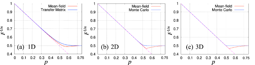
Figure 3: Mean-field results for the fidelity $F^{1/n}$ of 1D (a), 2D (b), and 3D (c) cluster states under depolarizing noise (red curves). The blue curves show the corresponding results obtained using the transfer matrix method for the 1D cluster state with $n=1000$ qubits (a), and Monte Carlo simulations for the 2D cluster state with $n_{x}=n_{y}=60$ (b), and the 3D cluster state with $n_{x}=n_{y}=n_{z}=6$ (c). The dashed magenta lines correspond to $1-p$.

The MF results of the fidelity in Figs. 3 (a), (b), and (c) indicate that $F^{1/n}$ exhibits a singularity point at $p_{\rm c}^{\rm MF}=0.535$ and $0.538$ for the 3D and 2D cluster states, respectively, while no such point is observed for the 1D cluster state. These singularities suggest that a phase transition occurs at $p_{\rm c}^{\rm MF}$. For $p<p_{\rm c}^{\rm MF}$, $F^{1/n}$ decreases linearly with $1-p$.

Since the MF free energy is larger than or equal to the actual free energy $\mathcal{F}_{\rm MF}\geq\mathcal{F}$ due to the Gibbs-Bogoliubov-Feynmann inequality B58 ; F55 , the mean-field partition function provides a lower bound for the actual partition function, that is, $\mathcal{Z}\geq\mathcal{Z}_{\rm MF}$. Consequently, fidelity within the MF approximation also provides a lower bound for actual fidelity, i.e., $F\geq F_{\rm MF}$, as shown in Figs. 3 (a), (b), and (c).

V Transfer matrix approach for 1D cluster state

The standard transfer matrix approach is applicable to the 1D cluster state under the periodic boundary condition shown in Fig. 4 (a). The Hamiltonian can be written as

$$\mathcal{H}=\sum_{i=1}^{n}h_{i}=\sum_{i=1}^{n/2}\tilde{h}_{2i-1,2i},$$ (21)

where we denote

$$h_{i}=\frac{1}{2}(1+s_{i})+\frac{1}{4}(1-s_{i})(1-s_{i-1}s_{i+1}),$$ (22)

$$\tilde{h}_{2i-1,2i}=h_{2i-1}+h_{2i}.$$ (23)

Note that $h_{i}=h_{i}(s_{i-1},s_{i},s_{i+1})$ and $\tilde{h}_{2i-1,2i}=\tilde{h}_{2i-1,2i}(s_{2i-2},s_{2i-1},s_{2i},s_{2i+1})$. The partition function can be written as

$$\mathcal{Z}=\sum_{s_{1}=\pm 1}\dots\sum_{s_{n}=\pm 1}\exp\left[-\beta\left(\sum_{i=1}^{n/2}\tilde{h}_{2i-1,2i}+c\right)\right]$$

$$=e^{-\beta c}\left[\prod_{j=1}^{n}\sum_{s_{j}=\pm 1}\right]\prod_{i=1}^{n/2}T((s_{2i-2},s_{2i-1}),(s_{2i},s_{2i+1})),$$ (24)

where the transfer matrix $T$ is given as

$$T((s_{2i-2},s_{2i-1}),(s_{2i},s_{2i+1}))$$

$$=\exp\left(-\beta\tilde{h}_{2i-1,2i}(s_{2i-2},s_{2i-1},s_{2i},s_{2i+1})\right).$$ (25)

Setting the order of the basis as $(1,1)$, $(1,-1)$, $(-1,1)$, and $(-1,-1)$, the explicit form of $T$ is

$$T=\begin{pmatrix}e^{-2\beta}&e^{-2\beta}&e^{-\beta}&e^{-2\beta}\\ e^{-\beta}&e^{-\beta}&e^{-2\beta}&e^{-\beta}\\ e^{-2\beta}&e^{-2\beta}&e^{-\beta}&e^{-2\beta}\\ e^{-2\beta}&e^{-2\beta}&e^{-\beta}&1\end{pmatrix}.$$ (26)

Note that one of the eigenvalues of the transfer matrix $T$ is zero, as the third row is identical to the first in Eq. (26). The remaining three eigenvalues are found to be real.

The partition function is obtained as

$$\mathcal{Z}=e^{-\beta c}~{\rm Tr}(T^{n/2})$$

$$=e^{-\beta c}(\lambda_{1}^{n/2}+\lambda_{2}^{n/2}+\lambda_{3}^{n/2}),$$ (27)

where $\lambda_{k}$ ($k=1,2,3$) are the nonzero eigenvalues of $T$. Thus, we obtain the fidelity as

$$F^{1/n}=(1-p)(\lambda_{1}^{n/2}+\lambda_{2}^{n/2}+\lambda_{3}^{n/2})^{1/n}.$$ (28)

In addition to fidelity, we also evaluate the internal energy $E=-\frac{d}{d\beta}\ln\mathcal{Z}$ and the specific heat $C=-\beta^{2}\frac{dE}{d\beta}$ of the classical spin system as functions of the noise parameter $p$. The internal energy, which corresponds to the expectation value of the Hamiltonian Eq. (19), reflects the averaged total number of Pauli $X$, $Y$, and $Z$ operators appearing in a stabilizer, since the mapped classical spin Hamiltonian assigns an energy equal to the number of such operators in each stabilizer.

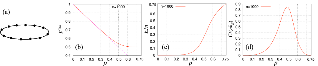
Figure 4: (a) 1D cluster state, where black dots represent qubits and black lines indicate $CZ$ gates. (b) Fidelity, (c) internal energy, and (d) specific heat as functions of the noise parameter $p$ for the 1D cluster state with number of qubits $n=1000$. The solid red curves in (b), (c), and (d) show the results obtained using the transfer matrix method. The dashed magenta line in (b) corresponds to $1-p$. $k_{\rm B}$ denotes the Boltzmann constant.

Figures 4 (b)–(d) show the results for the 1D cluster state obtained using the transfer matrix approach. As seen in Fig. 4 (b), the fidelity exhibits a smooth crossover from the pure state to the maximally mixed state around $p\simeq 0.5$. Correspondingly, the internal energy increases monotonically with $p$, and the specific heat shows a broad, non-divergent peak near $p\simeq 0.5$. These results indicate that no phase transition occurs in the 1D cluster state.

A phase transition is marked by non-analytic behavior of the free energy in the limit $n\to\infty$. In this limit, the partition function and the fidelity become $\mathcal{Z}\to e^{-\beta c}\lambda_{1}^{n/2}$ and $F^{1/n}\to(1-p)\lambda_{1}^{1/2}$, respectively, where $\lambda_{1}$ is the largest eigenvalue. The free energy, then, becomes

$$\mathcal{F}\to c-\frac{n}{2\beta}\ln\lambda_{1}.$$ (29)

Since $T$ has strictly positive matrix elements, $\lambda_{1}$ is positive and non-degenerate from the Perron-Frobenius theorem and hence $\mathcal{F}$ is analytic. Thus, we can conclude that no phase transition occurs in the fidelity.

The fidelity $F^{1/n}$ in Fig. 4 (b) deviates from and exceeds $1-p$ for $p\gtrsim 0.4$. This deviation arises from the second term in Eq. (7), which accounts for contributions from Pauli noise operators that coincide with stabilizers. Such contributions lead to the smooth crossover between the pure-state regime and the maximally mixed-state regime.

VI Monte Carlo approach for 2D and 3D cluster states

For 2D and 3D graph states, the fidelity can be computed by using the Monte Carlo method for the classical spin system. Our Monte Carlo calculation is based on the Metropolis algorithm.

We focus on graph states on uniform 2D and 3D $d$-regular graphs, where each vertex is connected to $d$ edges. A $d$-regular graph state is said to have degree $d$. Figures 5 (a)-(f) show 2D $d$-regular graph states for $3\leq d\leq 8$. The 4-regular graph state corresponds to the 2D cluster state. We note that the number of qubits in the transverse direction must be even when $d$ is odd under the periodic boundary condition.

A 3D $(d+2)$-regular graph state can be constructed by stacking 2D $d$-regular graph states and then connecting each qubit to its counterparts in the adjacent upper and lower layers via additional edges. In this way, the 3D cluster state (with degree 6) is obtained by stacking 2D cluster states (degree 4), while the 3D 5-regular graph state is constructed by stacking 2D 3-regular graphs.

VI.1 2D graph states

The results of the 2D cluster state are presented in Figs. 6 (a)-(c). As shown in Fig. 6 (a), $F^{1/n}$ for the 2D cluster state decreases linearly with $p$, similar to the 1D case, and continuously approaches the value of the maximally mixed state, $1/2$, at $p\simeq 1/2$. Although the transition from the linear regime to the constant regime is more abrupt than in the 1D case in Fig. 4 (b), it remains smooth even as the system size increases, indicating the absence of a phase transition. Consistent with this behavior, the internal energy increases smoothly with $p$, and the specific heat exhibits a relatively broad peak near $p=1/2$ that does not grow with the system size (see Figs. 6 (b) and (c)).

Figure 5: 2D $d$-regular graph states for $3\leq d\leq 8$. Each black dot and line indicate a qubit and $CZ$ gate, respectively.

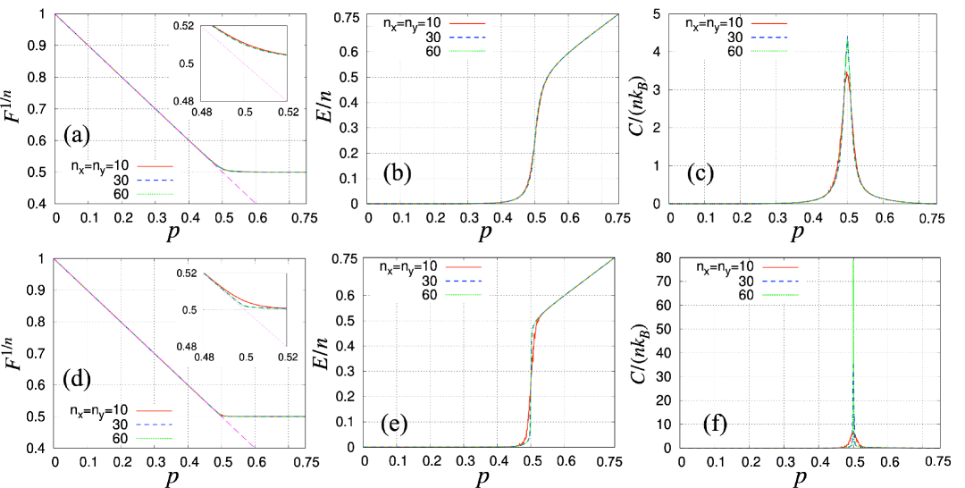
Figure 6: Fidelity ((a), (d)), internal energy ((b), (e)), and specific heat ((c), (f)) as functions of the noise parameter $p$, for the 2D cluster state ((a)–(c)) and the 2D 6-regular graph state ((d)–(f)). $n_{x}$ and $n_{y}$ denote the numbers of qubits of the 2D graph states in the $x$ and $y$ directions. The insets in (a) and (d) show magnified views of the corresponding plots. The dashed magenta lines in (a) and (d) correspond to $1-p$.

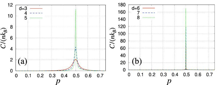
Figure 7: Specific heat of 2D uniform graph states with degree $d=3,4,5$ in (a) and $d=6,7,8$ in (b), plotted as functions of the noise parameter $p$, where we set the size of the graph states $n_{x}=n_{y}=60$.

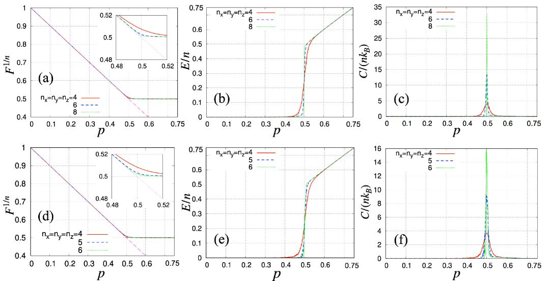
Figure 8: Fidelity ((a), (d)), internal energy ((b), (e)), and specific heat ((c), (f)) as functions of the noise parameter $p$, for the 3D 5-regular graph state ((a)–(c)) and the 3D cluster state ((d)–(f)). The insets in (a) and (d) show magnified views of the corresponding plots. The dashed magenta lines in (a) and (d) correspond to $1-p$.

To compare with the results for the 2D cluster state, Figs. 6 (d)–(f) show the corresponding results for the 6-regular graph state. In contrast to the 2D cluster state, the transition of $F^{1/n}$ from the linear regime to the plateau exhibits a sharp change at the critical value $p_{\rm c}\simeq 0.5$, indicating the occurrence of a phase transition. The internal energy shows a discontinuous jump from zero to a finite value $E/n\simeq 0.5$ at $p_{\rm c}$, which reflects a sudden proliferation of Pauli errors. The discontinuity of the internal energy, which corresponds to the latent heat for the classical spins, indicates that the phase transition is of first-order. The specific heat displays a pronounced peak at the same point. As the number of qubits increases, the jump in internal energy becomes more abrupt and the specific heat peak becomes sharper and higher, unlike the case of the 2D cluster state, where the peak remains broad and size-independent (see Figs. 6(e) and (f)).

In the presence of a phase transition, the pure state term $(1-p)^{n}$ in Eq. (7) dominates for $p$ smaller than $p_{\rm c}$, while for $p\geq p_{c}$ the contribution from Pauli noise, which is the second term in Eq. (7), abruptly becomes significant, driving the system toward the maximally mixed state. The phase transition arises from this sudden onset of noise effects.

Whether a phase transition occurs depends critically on the degree of the graph state. Figures 7 (a) and (b) show the specific heat for 2D $d$-regular graph states with $3\leq d\leq 8$. As $d$ increases, the peak of the specific heat becomes sharper and more pronounced. For graph states with $d\leq 5$, the peak remains broad and low, indicating the absence of a phase transition. In contrast, for $d\geq 6$, the specific heat grows and sharpens with increasing system size, clearly signaling the onset of a phase transition. These results suggest that phase transitions occur when the degree exceeds 5, while no transition is observed for degrees below 6.

When a phase transition occurs, since the fidelity is dominated by the pure state term $F=(1-p)^{n}$ for $p<p_{\rm c}$, it decreases more rapidly than in cases without a phase transition. Consequently, graph states with lower connectivity ($d\leq 5$), which exhibit a smooth crossover between the pure and maximally mixed states, are more robust against noise than highly connected ones ($d\geq 6$).

Interestingly, when the degree becomes excessively large, the phase transition disappears. For example, the fidelity for an $n$-qubit fully connected graph state, given by TTYYT23

$$F=\frac{1}{2}\left[\left(1-\frac{2}{3}p\right)^{n}+\left(\frac{2}{3}p\right)^{n}+\left(1-\frac{4}{3}p\right)^{n}\right]$$ (30)

does not exhibit any singularity in the limit $n\to\infty$. Determining the maximum degree at which a phase transition can still occur remains a question for future work.

VI.2 3D graph states

Figures 8 (a)–(f) present the results for the 3D 5-regular graph state and the 3D cluster state. While the 2D 5-regular graph state does not exhibit a phase transition, the 3D 5-regular graph state shows clear signs of a phase transition, as evidenced by the growing peak in the specific heat with increasing system size. This indicates that the occurrence of a phase transition depends not only on the degree but also on the dimensionality of the graph state. The results for the 3D cluster state, shown in Figs. 8 (d)–(f), further confirm the presence of a phase transition and reinforce the trend that phase transitions become more likely as degree increases. These results indicate that the dimensionality of the graph state significantly affects its robustness. That is, higher-dimensional graph states are more fragile to noise than low-dimensional ones.

VII Conclusion and discussion

In this work, we demonstrated that the fidelity of any graph state under IID Pauli noise can be mapped to the partition function of a classical spin system, which enables efficient evaluation of fidelity via statistical mechanical methods.

We found that fidelity undergoes a sharp phase transition driven by the abrupt onset of Pauli noise effects at the critical value of probability $p_{\rm c}\simeq 0.5$ for graph states on regular graphs with sufficiently high degree and dimensionality. Specifically, phase transitions appear for $d\geq 6$ in 2D and $d\geq 5$ in 3D. For 1D and lower-degree graphs in 2D, the fidelity exhibits a smooth crossover, indicating the absence of a phase transition.

We further found that robustness against noise is determined by the graph structure. Graph states with lower connectivity and dimensionality, which display a smooth crossover, tend to be more robust, while those with higher connectivity or dimensionality are more fragile. However, in the case of extreme connectivity—as in fully connected graphs—critical behavior is suppressed and robustness is restored.

Several open questions remain. First, while this study focused on depolarizing noise, it would be valuable to extend the analysis to other types of IID noise and correlated noise models. Second, the maximum degree of a regular graph state that can exhibit a fidelity phase transition remains to be determined. Third, it would be important to investigate whether the mapping of fidelity to the partition function of a classical spin model can be extended to other classes of stabilizer states. Finally, exploring the connection between noise robustness and computational ability as a resource state of MBQC is an interesting direction for future research.

APPENDIX A: Mean-field approximation

We perform a MF analysis to the classical spin system obtained by mapping the fidelity of graph states. We consider graph states under depolarizing noise that correspond to the Hamiltonian Eq. (19).

Classical spin $s_{i}$ can be written as $s_{i}=\langle s\rangle+\delta s_{i}$, where $\langle s\rangle$ denotes the average of $s_{i}$ and $\delta s_{i}$ denotes fluctuation from the average, which is assumed small. Within the first order of fluctuation, a product of spins can be written as

$$s_{i_{1}}s_{i_{2}}\cdots s_{i_{l}}=\langle s\rangle^{l}+\langle s\rangle^{l-1}\sum_{j=1}^{l}\delta s_{i_{j}}$$

$$=(1-l)\langle s\rangle^{l}+\langle s\rangle^{l-1}\sum_{j=1}^{l}s_{i_{j}}.$$ (31)

Using this formula, the MF Hamiltonian can be written as

$$\mathcal{H}_{\rm MF}=B(\langle s\rangle)\sum_{i=1}^{n}s_{i}+D(\langle s\rangle),$$ (32)

where the form of the functions $B(\langle s\rangle)$ and $D(\langle s\rangle)$ depend on the graph. For instance, their explicit forms for $d$-dimensional cluster states ($d=1,2,3$) are given as

$$B(\langle s\rangle)=\frac{1}{4}-\frac{k}{4}\langle s\rangle^{k-1}+\frac{k+1}{4}\langle s\rangle^{k},$$ (33)

$$D(\langle s\rangle)=\frac{3n}{4}+\frac{n(k-1)}{4}\langle s\rangle^{k}-\frac{nk}{4}\langle s\rangle^{k+1},$$ (34)

where $k\equiv 2d$ is the degree of $d$-dimensional cluster state.

The partition function of the mean-field Hamiltonian $\mathcal{Z}_{\rm MF}$ is given as

$$\mathcal{Z}_{\rm MF} =\sum_{s_{1}=\pm 1}\sum_{s_{2}=\pm 1}\dots\sum_{s_{n}=\pm 1}e^{-\beta({\mathcal{H}}_{\rm MF}+c)}$$

$$=e^{-\beta(D+c)}2^{n}\cosh^{n}(\beta B).$$ (35)

Thus, the self-consistent equation for $\langle s\rangle$ is given as

$$\langle s\rangle =\sum_{s_{1}=\pm 1}\sum_{s_{2}=\pm 1}\dots\sum_{s_{n}=\pm 1}s_{i}\frac{e^{-\beta({\mathcal{H}}_{\rm MF}+c)}}{{\mathcal{Z}}_{\rm MF}}$$

$$=-\tanh(\beta B).$$ (36)

Solving the above self-consistent equation, magnetization $\langle s\rangle$ can be determined. If multiple solutions are found, the stable solution has minimum free energy. The mean-field free energy is given as

$${\mathcal{F}}_{\rm MF}=D+c-\frac{n}{\beta}\ln\left[2\cosh(\beta B)\right].$$ (37)

References

- (1) N. Shettell and D. Markham, Graph States as a Resource for Quantum Metrology, Phys. Rev. Lett. 124, 110502 (2020).
- (2) K. Azuma, K. Tamaki, and H.-K. Lo, All-photonic quantum repeaters, Nat. Commun. 6, 6787 (2015).
- (3) D. Schlingemann and R.F. Werner, Quantum error-correcting codes associated with graphs, Phys. Rev. A 65, 012308 (2001).
- (4) R. Raussendorf and H. J. Briegel, A One-Way Quantum Computer, Phys. Rev. Lett. 86, 5188 (2001).
- (5) R. Raussendorf, D. E. Browne, H. J. Briegel, Measurement-based quantum computation on cluster states, Phys. Rev. A 68, 022312 (2003).
- (6) S. Spilla, R. Migliore, M. Scala, and A. Napoli, GHZ state generation of three Josephson qubits in the presence of bosonic baths, J. Phys. B: At. Mol. Opt. Phys. 45, 065501 (2012).
- (7) K. L. Brown, C. Horsman, V. Kendon, and W. J. Munro, Layer-by-layer generation of cluster states, Phys. Rev. A 85, 052305 (2012).
- (8) C. Monroe, R. Raussendorf, A. Ruthven, K. R. Brown, P. Maunz, L.-M. Duan, and J. Kim, Large-scale modular quantum-computer architecture with atomic memory and photonic interconnects, Phys. Rev. A 89, 022317 (2014).
- (9) K. Inaba, Y. Tokunaga, K. Tamaki, K. Igeta, and M. Yamashita, High-Fidelity Cluster State Generation for Ultracold Atoms in an Optical Lattice, Phys. Rev. Lett. 112, 110501 (2014).
- (10) M. Gimeno-Segovia, P. Shadbolt, D. E. Browne, and T. Rudolph, From Three-Photon Greenberger-Horne-Zeilinger States to Ballistic Universal Quantum Computation, Phys. Rev. Lett. 115, 020502 (2015).
- (11) C.-Y. Lu, X.-Q. Zhou, O. Gühne, W.-B. Gao, J. Zhang, Z.-S. Yuan, A. Goebel, T. Yang, and J.-W. Pan, Experimental entanglement of six photons in graph states, Nat. Phys. 3, 91 (2007).
- (12) Y. Tokunaga, S. Kuwashiro, T. Yamamoto, M. Koashi, and N. Imoto, Generation of High-Fidelity Four-Photon Cluster State and Quantum-Domain Demonstration of One-Way Quantum Computing, Phys. Rev. Lett. 100, 210501 (2008).
- (13) X.-C. Yao, T.-X. Wang, P. Xu, H. Lu, G.-S. Pan, X.-H. Bao, C.-Z. Peng, C.-Y. Lu, Y.-A. Chen, and J.-W. Pan, Observation of eight-photon entanglement, Nat. Photonics 6, 225 (2012).
- (14) X.-C. Yao, T.-X. Wang, H.-Z. Chen, W.-B. Gao, A. G. Fowler, R. Raussendorf, Z.-B. Chen, N.-L. Liu, C.-Y. Lu, Y.-J. Deng, Y.-A. Chen, and J.-W. Pan, Experimental demonstration of topological error correction, Nature (London) 482, 489 (2012).
- (15) X.-L. Wang, L.-K. Chen, W. Li, H.-L. Huang, C. Liu, C. Chen, Y.-H. Luo, Z.-E. Su, D. Wu, Z.-D. Li, H. Lu, Y. Hu, X. Jiang, C.-Z. Peng, L. Li, N.-L. Liu, Y.-A. Chen, C.-Y. Lu, and J.-W. Pan, Experimental Ten-Photon Entanglement, Phys. Rev. Lett. 117,210502 (2016).
- (16) X.-L. Wang, Y.-H. Luo, H.-L. Huang, M.-C. Chen, Z.-E. Su, C. Liu, C. Chen, W. Li, Y.-Q. Fang, X. Jiang, J. Zhang, L. Li, N.-L. Liu, C.-Y. Lu, and J.-W. Pan, 18-Qubit Entanglement with Six Photons’ Three Degrees of Freedom, Phys. Rev. Lett. 120, 260502 (2018).
- (17) Y. Wang, Y. Li, Z.-q. Yin, and B. Zeng, 16-qubit IBM universal quantum computer can be fully entangled, npj Quantum Information 4, 46 (2018).
- (18) M. Gong, M.-C. Chen, Y. Zheng, S. Wang, C. Zha, H. Deng, Z. Yan, H. Rong, Y. Wu, S. Li, F. Chen, Y. Zhao, F. Liang, J. Lin, Y. Xu, C. Guo, L. Sun, A. D. Castellano, H. Wang, C. Peng, C.-Y. Lu, X. Zhu, and J.-W. Pan, Genuine 12-Qubit Entanglement on a Superconducting Quantum Processor, Phys. Rev. Lett. 122, 110501 (2019).
- (19) G. J. Mooney, C. D. Hill, and L. C. L. Hollenberg, Entanglement in a 20-Qubit Superconducting Quantum Computer, Sci. Rep. 9, 13465 (2019).
- (20) C. Roh, G. Gwak, Y.-D. Yoon, and Y.-S. Ra, Generation of three-dimensional cluster entangled state arXiv:2309.05437 (2023).
- (21) M. Hayashi and T. Morimae, Verifiable Measurement-Only Blind Quantum Computing with Stabilizer Testing, Phys. Rev. Lett. 115, 220502 (2015).
- (22) T. Morimae, D. Nagaj, and N. Schuch, Quantum proofs can be verified using only single-qubit measurements, Phys. Rev. A 93, 022326 (2016).
- (23) K. Fujii and M. Hayashi, Verifiable fault tolerance in measurement-based quantum computation, Phys. Rev. A 96, 030301(R) (2017).
- (24) S. Pallister, N. Linden, and A. Montanaro, Optimal Verification of Entangled States with Local Measurements, Phys. Rev. Lett. 120, 170502 (2018).
- (25) M. Hayashi and M. Hajdušek, Self-guaranteed measurement-based quantum computation, Phys. Rev. A 97, 052308 (2018).
- (26) Y. Takeuchi and T. Morimae, Verification of Many-Qubit States, Phys. Rev. X 8, 021060 (2018).
- (27) Y. Takeuchi, A. Mantri, T. Morimae, A. Mizutani, and J. F. Fitzsimons, Resource-efficient verification of quantum computing using Serfling’s bound, npj Quantum Information 5, 27 (2019).
- (28) H. Zhu and M. Hayashi, Efficient Verification of Pure Quantum States in the Adversarial Scenario, Phys. Rev. Lett. 123, 260504 (2019).
- (29) H. Zhu and M. Hayashi, General framework for verifying pure quantum states in the adversarial scenario, Phys. Rev. A 100, 062335 (2019).
- (30) D. Markham and A. Krause, A Simple Protocol for Certifying Graph States and Applications in Quantum Networks, Cryptography 4, 3 (2020).
- (31) N. Dangniam, Y.-G. Han, and H. Zhu, Optimal verification of stabilizer states, Phys. Rev. Research 2, 043323 (2020).
- (32) Z. Li, H. Zhu, and M. Hayashi, Robust and efficient verification of measurement-based quantum computation, arXiv:2305.10742.
- (33) K. Akimoto, S. Tsuchiya, R. Yoshii, and Y. Takeuchi, Passive verification protocol for thermal graph states, Phys. Rev. A 106, 012405 (2022).
- (34) T. Tanizawa, Y. Takeuchi, S. Yamashika, R. Yoshii, and S. Tsuchiya, Fidelity-estimation method for graph states with depolarizing noise, Phys. Rev. Research 5, 043260 (2023).
- (35) R. Fan, Y. Bao, E. Altman, and A. Vishwanath, Diagonostics of Mixed-State Topological Order and Breakdown of Quantum Memory, PRX Quantum 5, 020343 (2024).
- (36) A. Lyons, Understanding Stabilizer Codes Under Local Decoherence Through A General Statistical Mechanics Mapping, arXiv:2403.03955.
- (37) Y. Gao and Y. Ashida, Two-dimensional symmetry-protected topological phases and transitions in open quantum system, Phys. Rev. B 109, 195420 (2024).
- (38) H. Yamasaki and S. Subramanian, Constant-time one-shot testing of large-scale graph states, arXiv:2201.11127 (2022).
- (39) M. A. Nielsen and I. L. Chuang, Quantum Computation and Quantum Information (Cambridge University Press, Cambridge, 2000).
- (40) N. N. Bogoliubov, A variation principle in the problem of many bodies, Dokl. Akad. Nauk SSSR 119, 244 (1958).
- (41) R. P. Feynman, Slow Electrons in a Polar Crystal, Phys. Rev. 97, 660 (1955).