Noncoincidence $f(Q)$-Cosmology with Dark Matter Coupled to Gravity

Abstract

We investigate FLRW cosmology in the framework of symmetric teleparallel $f(Q)$ gravity with a nonminimal coupling between dark matter and the gravitational field. In the noncoincidence gauge, the field equations admit an equivalent multi-scalar field representation, which we investigate the phase-space using the Hubble-normalization approach. We classify all stationary points for arbitrary function $f(Q)$ and we discuss the physical properties of the asymptotic solutions. For the power-law theory, we perform a detailed stability analysis and show that the de Sitter solution is the unique future attractor, while the matter-dominated point appears as a saddle point. Moreover, there exist a family of scaling solutions that can be related to inflationary dynamics. In contrast with uncoupled $f(Q)$ models, the presence of the coupling introduces a viable matter-dominated era alongside late-time accelerated expansion. Our study shows that the coupling function plays a crucial role in cosmological dynamics in $f(Q)$ gravity.

I Introduction

Recently, Symmetric Teleparallel General Relativity (STEGR) Nester:1998mp and its generalizations have attracted considerable attention in cosmology as promising frameworks for describing the dynamical structure of the universe.

In General Relativity (GR) the fundamental object associated with the gravitational field is the Levi-Civita connection. In contrast, in STEGR the corresponding role is played by the nonmetricity tensor, defined through a symmetric and flat connection revh . Although GR and STEGR are equivalent, this equivalence breaks down when scalar fields or nonlinear extensions of the geometric scalars are introduced into the gravitational Action Koivisto2 ; Koivisto3 ; Baha1 ; sc1 ; sc3 ; mf1 ; mf2 ; mf3 ; Shabani:2025qxn . For instance, the $f\left(R\right)$ and $f\left(Q\right)$ theories of gravity are equivalent only when the functional dependence is linear, that is, the theories are equivalent with GR or STEGR respectively. This simple observation has been omitted in a series of studies as discussed recently in tel .

The choice of connection within the symmetric teleparallel theory is not unique, and selecting an appropriate one is crucial for ensuring the physical viability of the model and for defining the gravitational theory itself. As discussed in detail in dd2 , a number of studies in the literature have employed nonphysical connections in the investigation of static spherically symmetric spacetimes. On the other hand, in dd4 it was shown that in a Kantowski-Sachs geometry tilted fluid components can be supported, in contrast with GR where this feature is not possible for such an anisotropic background.

In modern cosmology, where spacetime is usually modeled by the isotropic and homogeneous Friedmann-Lemaître-Robertson-Walker (FLRW) geometry, there exist four possible connections consistent with being symmetric, flat, and compatible with the isometries of the background Hohmann ; fq4 . Three of these correspond to the spatially flat case, while the fourth applies to the nonzero-curvature case. The associated degrees of freedom of $f\left(Q\right)$ theory have been investigated in detail in the literature. In particular, the field equations admit a minisuperspace description an3 . It was found that when the connection is defined in the noncoincidence gauge, additional dynamical degrees of freedom appear, which can be interpreted as scalar fields an2 . On the other hand, when the coincidence gauge is adopted, the resulting cosmological equations coincide with those of $f\left(T\right)$ teleparallel gravity tel1 .

Within the coincidence gauge, observational tests of $f\left(Q\right)$ theory have been presented in ob1 ; ob2 ; ob3 . More recently, the issues of structure growth and the $H_{0}$ and $S_{8}$ tensions were examined in ob4 ; ob5 . The effects of adopting the noncoincidence connection on the description of late-time acceleration were analyzed in an4 . In particular, by applying the latest Baryonic Acoustic Oscillation (BAO) data from the DESI DR2 release des4 ; des5 ; des6 , it was found that this cosmological model challenges $\Lambda$CDM and related theories formulated in the coincidence gauge.

In ppr1 ; ppr2 it was shown that $f\left(Q\right)$ gravity suffers from strong coupling or the appearance of ghosts at the level of cosmological perturbations. Nevertheless, these problems can be avoided when the matter sector is coupled to the gravitational field directly in the Action Integral. This type of interaction is the focus of the present work, where we restrict attention to the background dynamics. Specifically, we perform a detailed phase-space analysis of the cosmological field equations in the presence of a coupling function. The stationary points are identified and used to reconstruct the possible cosmological histories supported by the theory.

Because of the nonlinearity of the gravitational field equations, phase-space methods provide a powerful tool for understanding the evolution of physical properties in cosmological models cop1 . Such analyses have been widely applied in various modified gravity theories ex1 ; ex2 ; ex3 ; ex4 ; ex5 ; ex6 ; ex7 ; ex8 ; ex9 ; ex10 , yielding valuable information on constraints for free parameters and on the behavior of the initial value problem ex11 ; ex12 . A detailed analysis of the phase-space of $f\left(Q\right)$ cosmology was carried out in an1 , where it was shown that different choices of connection lead to distinct sets of field equations and hence to different cosmic evolutions. For additional work on phase-space analyses in modified STEGR, we refer the reader to fq5 ; fq6 ; fq7 ; anc1 ; anc2 and references therein.

The purpose of this study is to investigate the impact of a coupling function between dark matter and gravity on the background dynamics and to assess the physical viability of the theory. The structure of the paper is as follows.

In Section II, we briefly review STEGR and its generalization, the $f\left(Q\right)$-theory. The cosmological model under consideration is introduced in Section III, where we examine a coupling between the matter source and the gravitational field. The coupling function is defined in such a way that, in the scalar-field representation, the field equations take their simplest form. Our analysis is carried out in the context of the noncoincident connection, where the connection introduces nontrivial dynamical degrees of freedom within the field equations. The corresponding cosmological field equations are equivalent to a multi-scalar field gravitational theory.

The existence of cosmological solutions of particular interest is investigated in Section IV. Specifically, we focus on the power-law solution describing the matter-dominated era and on the de Sitter universe. In Section V, we present a detailed dynamical analysis of the cosmological field equations and explore the impact of the matter-gravity coupling on the global cosmic history. We determine the stationary points for an arbirtary function $f\left(Q\right)$, nevertheless we investigate the stability properties for the special case of the power-law $f\left(Q\right)\simeq Q^{\frac{n}{n-1}}$ model. Finally, in Section VI, we summarize our findings and present our conclusions.

II Symmetric Teleparallel Gravity

Consider a four-dimensional manifold $M^{4}$, equipped with a metric tensor $g_{\mu\nu}$ and a generic affine connection $\Gamma_{\mu\nu}^{\kappa}$, which defines the covariant derivative $\nabla_{\lambda}$. The generic connection can be decomposed into three components Eisenhart .

The Levi-Civita connection $\mathring{\Gamma}_{\mu\nu}^{\kappa}$, defined by the metric tensor

$$\mathring{\Gamma}_{\mu\nu}^{\kappa}=\frac{1}{2}g^{\kappa\lambda}\left(g_{\mu\lambda,\nu}+g_{\lambda\nu,\mu}-g_{\mu\nu,\lambda}\right),$$ (1)

the torsion tensor $\mathrm{T}_{\mu\nu}^{\kappa}$, defined as the antisymmetric part of the connection

$$\mathrm{T}_{\mu\nu}^{\kappa}=\Gamma_{\mu\nu}^{\kappa}-\Gamma_{\nu\mu}^{\kappa},$$ (2)

and the nonmetricity tensor $Q_{\lambda\mu\nu}$, which measures the failure of the connection to preserve the metric

$$Q_{\lambda\mu\nu}=\partial_{\lambda}g_{\mu\nu}-\Gamma_{\lambda\mu}^{\sigma}g_{\sigma\nu}-\Gamma_{\lambda\nu}^{\sigma}g_{\mu\sigma}.$$ (3)

Consequently, the generic connection $\Gamma_{\mu\nu}^{\kappa}$ is expressed as follows Eisenhart :

$$\Gamma_{\mu\nu}^{\kappa}=\mathring{\Gamma}_{\mu\nu}^{\kappa}+\mathrm{T}_{\mu\nu}^{\kappa}+Q_{\;\mu\nu}^{\kappa}.$$ (4)

Each component of the connection defines a fundamental tensor that characterizes the geometric structure of the manifold $M^{4}$.

In GR, the gravitational field is described solely by the Levi-Civita connection, i.e., $\Gamma_{\mu\nu}^{\kappa}=\mathring{\Gamma}_{\mu\nu}^{\kappa}$, and the dynamics are given by the Riemann curvature tensor:

$$R_{\;\lambda\mu\nu}^{\kappa}=\partial_{\mu}\Gamma_{\lambda\nu}^{\kappa}-\partial_{\nu}\Gamma_{\lambda\mu}^{\kappa}+\Gamma_{\lambda\nu}^{\sigma}\Gamma_{\mu\sigma}^{\kappa}-\Gamma_{\lambda\mu}^{\sigma}\Gamma_{\nu\sigma}^{\kappa}.$$ (5)

In contrast, in TEGR, the connection is taken to be purely antisymmetric, i.e., $\Gamma_{\mu\nu}^{\kappa}=\mathrm{T}_{\mu\nu}^{\kappa}$, and the gravitational field is described by the torsion tensor. Finally, in STEGR, the connection is assumed to be flat $R_{\;\lambda\mu\nu}^{\kappa}=0$ and symmetric $\mathrm{T}_{\mu\nu}^{\kappa}=0$, implying that only the nonmetricity tensor contributes to the gravitational field $\Gamma_{\mu\nu}^{\kappa}=Q_{\;\mu\nu}^{\kappa}.$

The analogue of the Einstein-Hilbert action in STEGR is given by Nester:1998mp

$$S_{Q}=\int d^{4}x\sqrt{-g}Q,$$ (6)

where the nonmetricity scalar $Q$ is defined as

$$Q=Q_{\lambda\mu\nu}P^{\lambda\mu\nu},$$

and $P_{\;\mu\nu}^{\lambda}$ is the the conjugate tensor with definition

$$P_{\;\mu\nu}^{\lambda}=-\frac{1}{4}Q_{\;\mu\nu}^{\lambda}+\frac{1}{2}Q_{\;(\mu\nu)}^{\lambda}+\frac{1}{4}\left(Q^{\lambda}-\bar{Q}^{\lambda}\right)g_{\mu\nu}-\frac{1}{4}\delta_{(\mu}^{\lambda}Q_{\nu)}.$$ (7)

Parentheses denote symmetrization: $A_{(\mu\nu)}=\frac{1}{2}(A_{\mu\nu}+A_{\nu\mu})$; $Q_{\mu}=Q_{\mu\nu}^{\;\;\;\nu}$, $\bar{Q}_{\mu}=Q_{\;\mu\nu}^{\nu}$, and $\delta_{\nu}^{\mu}$ is the Kronecker delta.

II.1 $f\left(Q\right)$-gravity

Introducing nonlinear functions of the nonmetricity scalar $Q$ in the action (6) leads to the family of $f(Q)$-gravity theories, with the action Koivisto2 ; Koivisto3

$$S_{f(Q)}=\int d^{4}x\sqrt{-g}f(Q).$$ (8)

In the absence of matter, variation of the action (8) with respect to the metric yields the field equations revh

$$\frac{2}{\sqrt{-g}}\nabla_{\lambda}\left(\sqrt{-g}f_{\;\mu\nu}^{\prime\lambda}\right)-\frac{f(Q)}{2}g_{\mu\nu}+f^{\prime}(Q)\left(P_{\mu\rho\sigma}Q_{\nu}^{\;\rho\sigma}-2Q_{\rho\sigma\mu}P_{\;\;\;\nu}^{\rho\sigma}\right)=0,$$ (9)

where $f^{\prime}(Q)=\frac{df}{dQ}$. Variation with respect to the connection yields the equation of motion

$$\nabla_{\mu}\nabla_{\nu}\left(\sqrt{-g}f^{\prime}\left(Q\right)P_{\;\;\;\sigma}^{\mu\nu}\right)=0.$$ (10)

This equation is trivially satisfied in the so-called coincidence gauge, where the connection vanishes. However, as discussed in various gravitational models, $f(Q)$-gravity recovers the GR limit only when a non-coincidence gauge is employed anc3 . Therefore, equation (10) plays a crucial role in the gravitational dynamics ndim1 . For a recent discussion we refer the reader to dial1 .

III Matter Coupled to Gravity

On cosmological scales, the universe is assumed to be isotropic and homogeneous, and is described by the FLRW metric with the line element

$$ds^{2}=-N^{2}(t)\,dt^{2}+a^{2}(t)\left(dx^{2}+dy^{2}+dz^{2}\right),$$ (11)

where $N(t)$ is the lapse function and $a(t)$ is the scale factor. For this line element there are three families of connections which lead to different cosmological models Hohmann ; fq4 . In this work, we consider the nontrivial affine connection with the following nonzero components:

$$\Gamma_{tt}^{t}=\frac{\ddot{\psi}(t)}{\dot{\psi}(t)}+\dot{\psi}(t),$$ (12)

$$\Gamma_{tr}^{r}=\Gamma_{rt}^{r}=\Gamma_{t\theta}^{\theta}=\Gamma_{\theta t}^{\theta}=\Gamma_{t\varphi}^{\varphi}=\Gamma_{\varphi t}^{\varphi}=\dot{\psi}(t).$$

The nonmetricity scalar $Q$ is calculated as

$$Q=-6H^{2}+\frac{3\dot{\psi}}{N}\left(3H-\frac{\dot{N}}{N^{2}}\right)+\frac{3\ddot{\psi}}{N^{2}},$$ (13)

where $H=\frac{1}{N}\frac{\dot{a}}{a}$ is the Hubble parameter.

It has been shown that this connection leads to cosmological dynamics with de Sitter behavior as an attractor, even without introducing a cosmological constant an1 ; dut1 , unlike the case with the coincidence connection. Moreover, inflationary solutions can be realized within this framework, as the theory is dynamically equivalent to a two-scalar field quintom-like gravitational model an2 . Recently, in an4 it was found that the geometrodynamical degrees of freedom introduced by this noncoincident connection can describe the late-time acceleration of the universe. The $\Lambda$CDM limit within the $f\left(Q\right)$-gravity for this connection was examined before in saik . On the other hand, this connection has been applied to investigate the evolution of the anisotropies in a homogeneous Bianchi I universe saik2 .

In this work, we introduce the matter Lagrangian $L_{m}=\rho_{m}$, representing an ideal pressureless fluid that models dark matter. The coupling to gravity is described by the action

$$S_{f(Q)}=\int d^{4}x\sqrt{-g}\left[f(Q)-\alpha f^{\prime}(Q)L_{m}\right],$$ (14)

such that in the limit $f(Q)\sim Q$, general relativity is recovered. Such interacting models have been examined before in other modified theories of gravity, see for instance fr1 ; fr2 ; fr3 . In our consideration the interacting function has been introduced in a way such that to introduce the minimum nonlinear terms in the cosmological field equations.

Assuming dark matter behaves as a pressureless fluid, we take $L_{m}=\rho_{m0}a^{-3}$. Introducing a Lagrange multiplier $\lambda$, the action becomes

$$S_{f(Q)}=\int d^{4}x\sqrt{-g}\left\{f(Q)+\lambda\left[Q-\left(-6H^{2}+\frac{3\dot{\psi}}{N}\left[3H-\frac{\dot{N}}{N^{2}}\right]+\frac{3\ddot{\psi}}{N^{2}}\right)\right]-\alpha f^{\prime}(Q)\rho_{m0}a^{-3}\right\},$$ (15)

where $\lambda=-f^{\prime}(Q)$.

After integrating by parts, the point-like action becomes

$$S_{f(Q)}=\int L_{f(Q)}(N,a,\dot{a},\phi,\dot{\phi},\psi,\dot{\psi})\,dt,$$ (16)

with the Lagrangian an3

$$L_{f(Q)}=-\frac{3}{N}\phi a\dot{a}^{2}-\frac{3}{2N}a^{3}\dot{\phi}\dot{\psi}+Na^{3}V(\phi)-\beta N\phi,$$ (17)

where $\beta=\alpha\rho_{m0}$, $\phi=f^{\prime}(Q)$, and the potential is defined as $V(\phi)=f(Q)-Qf^{\prime}(Q)$. The inverse relation is given by

$$f(Q)=V(\phi(Q))-\phi(Q)V_{,\phi}(Q).$$ (18)

Within the minisuperspace description it is easy to see that under a conformal transformation, the coupling function between the gravitational field and the matter is eliminated.

The cosmological field equations follow from the variation of the latter point-like Lagrangian with respect to the dynamical variables $\left\{N,a,\phi,\psi\right\}$. Setting $N=1$ we calculate the equations

$$3\phi H^{2}+\frac{3}{2}\dot{\phi}\dot{\psi}+V(\phi)-\beta\phi a^{-3} =0,$$ (19)

$$\phi(2\dot{H}+3H^{2})+2H\dot{\phi}-\frac{3}{2}\dot{\phi}\dot{\psi}+V(\phi) =0,$$ (20)

$$\ddot{\phi}+3H\dot{\phi} =0,$$ (21)

$$\ddot{\psi}-2H^{2}+3H\dot{\psi}+\frac{2}{3}V_{,\phi} =-\frac{2}{3}\beta a^{-3}.$$ (22)

Solving for the higher-order derivatives we find

$$\dot{H} =-\frac{H\dot{\phi}}{\phi}-\frac{3}{2}H^{2}-\frac{V(\phi)}{2\phi}+\frac{3\dot{\psi}\dot{\phi}}{4\phi},$$ (23)

$$\ddot{\phi} =-3H\dot{\phi},$$ (24)

$$\ddot{\psi} =-\frac{2\beta}{3a^{3}}-3H\dot{\psi}+2H^{2}-\frac{2}{3}V^{\prime}(\phi).$$ (25)

The modified Friedmann equations can be written in the equivalent form

$$3H^{2} =\frac{1}{\phi}\left(\rho_{f\left(Q\right)}+\rho_{m}\right),$$ (26)

$$2\dot{H}+3H^{2} =-\frac{1}{\phi}p_{f\left(Q\right)},$$ (27)

where

$$\rho_{f\left(Q\right)} =-\frac{3}{2}\dot{\phi}\dot{\psi}-V\left(\phi\right),$$ (28)

$$p_{f\left(Q\right)} =-\frac{3}{2}\dot{\phi}\dot{\psi}+2H\dot{\phi}+V\left(\phi\right),$$ (29)

are the geometric fluid components related to the $f\left(Q\right)$-gravity, and $\rho_{m}=\beta\phi a^{-3}$, is the energy density for the matter source, which satisfies the conservation law

$$\dot{\rho}_{m}+3H\rho_{m}=\rho_{m}\left(\ln\phi\right)^{\cdot}\text{.}$$ (30)

In the following, we investigate the impact of the coupling parameter $\beta$ on the cosmological dynamics of $f(Q)$-gravity.

IV Exact Solutions

We examine the existence of two exact cosmological solutions of special interests, the power-law solution, $a\left(t\right)=a_{0}t^{p}$, with Hubble function $H\left(t\right)=\frac{p}{t}$, and the de Sitter solution $a\left(t\right)=a_{0}e^{H_{0}t}$ with constant Hubble function $H\left(t\right)=H_{0}$. The power-law solution can describe a radiation epoch, for $p=\frac{1}{2}$, or the matter dominated era, for $p=\frac{2}{3}$.

IV.1 Power-law Solution

Substituting $H(t)=\frac{p}{t}$ into the cosmological field equations, we find that the system admits the following solution:

$$\phi(t) =\phi_{1}t^{1-3p}+\phi_{0},$$ (31)

$$\dot{\psi}(t) =-\frac{\phi_{0}\left(2pt^{-2+3p}-\beta\right)+\phi_{1}\left(6p^{2}t^{-1}-\beta t^{1-3p}\right)}{3\phi_{1}(1-3p)},$$ (32)

$$V(t) =(1-3p)p\phi_{0}t^{-2}+\frac{\beta}{2}t^{-6p}\left(\phi_{0}t^{3p}+\phi_{1}t\right).$$ (33)

The corresponding scalar potential $V(\phi)$ can be reconstructed as

$$V(\phi) =(3p-1)\phi_{0}\left(\phi_{1}(\phi-\phi_{0})\right)^{\frac{2}{3p-1}}$$

$$~~~~~~-\frac{\beta}{2}\left(\phi_{1}(\phi-\phi_{0})\right)^{1+\frac{1}{3p-1}}\phi.$$ (34)

Indeed, in the absence of the interacting term, that is, $\beta=0$, the latter potential leads to the power-law function for the $f\left(Q\right)$-model as discussed before in ndim1 .

IV.2 de Sitter Solution

For the de Sitter case, where $H(t)=H_{0}$ is constant, the field equations admit the solution:

$$\phi(t) =\phi_{1}e^{-3H_{0}t}+\phi_{0},$$ (35)

$$\dot{\psi}(t) =\frac{2}{3}H_{0}-\frac{\beta}{9H_{0}}\left(e^{-3H_{0}t}+\frac{\phi_{0}}{\phi_{1}}\right),$$ (36)

$$V(t) =-3H_{0}^{2}\phi_{0}-\frac{\beta}{2}e^{-6H_{0}t}\left(e^{3H_{0}t}\phi_{0}+\phi_{1}\right).$$ (37)

The scalar potential $V(\phi)$ takes the form

$$V(\phi)=-3H_{0}^{2}\phi_{0}+\frac{\beta}{2\phi_{1}}(\phi-\phi_{0})\phi.$$ (38)

Consequently, the closed-form expression for the function $f(Q)$ is

$$f(Q)=f_{1}\frac{\phi_{1}}{\sqrt{2\beta}}Q-\frac{\phi_{1}}{2\beta}Q^{2}+\frac{\phi_{1}f_{1}^{2}}{4}-3H_{0}^{2}\phi_{0}.$$ (39)

Therefore, only when $\phi_{1}=0\,,$ that is, $\phi\left(t\right)=\phi_{0}$, the interacting term can be omitted, i.e. $\beta=0$, which leads to the case $f\left(Q\right)=-3H_{0}^{2}\phi_{0}$, that is $Q$ is a constant scalar ndim1 .

In the following, we perform a detailed analysis for the phase-space for the cosmological field equations. Such analysis will provide us with important information about the nature of the interacting term in the cosmic evolution.

V Cosmological Dynamics

A systematic exploration of the dynamical structure of scalar–tensor models offers profound insights into their cosmological behavior. By recasting the field equations into an autonomous system with suitable dimensionless variables, one gains direct access to the global phase–space geometry. This framework makes it possible to identify fixed points such as attractors, repellers, and saddle points that determine the asymptotic evolution of the universe.

V.1 Dimensionless Variables and Dynamical System

We work within the $H$-normalization approach and we define the following dimensionless variables

$$\begin{pmatrix}\Omega_{m}\\ \Omega_{V}\\ x_{\phi}\\ x_{\psi}\\ \lambda\end{pmatrix}=\begin{pmatrix}\frac{1}{3a^{3}H^{2}}\\ \frac{V(\phi)}{3H^{2}\phi}\\ \frac{\dot{\phi}}{H\phi}\\ \frac{\dot{\psi}}{2H}\\ \frac{\phi V^{\prime}(\phi)}{V(\phi)}\end{pmatrix}$$ (40)

These variables quantify the normalized energy densities and field velocities. $\Omega_{m}$ describes the matter contribution, $\Omega_{V}$ the potential energy contribution, $x_{\phi}$ is the normalized velocity of the scalar field $\phi$ and $x_{\psi}$ defines the normalized velocity of the scalar field $\psi$.

$$\lambda =\frac{\phi V^{\prime}(\phi)}{V(\phi)},$$ (41)

$$g(\lambda) =\frac{\phi^{2}V^{\prime\prime}(\phi)}{V(\phi)}-\frac{\phi^{2}V^{\prime 2}}{V(\phi)^{2}}+\frac{\phi V^{\prime}(\phi)}{V(\phi)}.$$ (42)

The first modified Friedmann equation (19) is expressed as the algebraic constraint

$$x_{\psi}x_{\phi}-\beta\Omega_{m}+\Omega_{V}+1=0.$$ (43)

The latter constraint allows to reduce by one the dimension of the dynamical system.

Using the e-folding number $N=\ln a$ as the time variable, the autonomous system becomes

$$\frac{d}{dN}\begin{pmatrix}\Omega_{V}\\ x_{\phi}\\ x_{\psi}\\ \lambda\end{pmatrix}=\begin{pmatrix}\Omega_{V}\left(\lambda x_{\phi}-3x_{\psi}x_{\phi}+x_{\phi}+3\Omega_{V}+3\right)\\ -\frac{3}{2}x_{\phi}\left(x_{\psi}x_{\phi}-\Omega_{V}+1\right)\\ -\lambda\Omega_{V}-\frac{3x_{\psi}^{2}x_{\phi}}{2}+\frac{1}{2}x_{\psi}\left(4x_{\phi}+3\Omega_{V}-3\right)+\Omega_{V}+2\\ x_{\phi}g(\lambda)\end{pmatrix}.$$ (44)

Function $g(\lambda)$ is defined as

$$g(\lambda\left(\phi\right))=\frac{\phi^{2}V^{\prime\prime}(\phi)}{V(\phi)}-\frac{\phi^{2}V^{\prime 2}}{V(\phi)^{2}}+\frac{\phi V^{\prime}(\phi)}{V(\phi)}.$$ (45)

The evolution equation for $\Omega_{m}$ is decoupled as follows

$$\frac{d}{dN}\Omega_{m}=-\left((3x_{\psi}-2)x_{\phi}-3\Omega_{V}\right)\left(x_{\psi}x_{\phi}+\Omega_{V}+1\right),$$ (46)

which confirms that $\Omega_{m}$ is evolving once the other variables are known.

Furthermore, in terms of the new variables, the effective equation of state parameter $w_{eff}=-1-\frac{2}{3}\frac{\dot{H}}{H^{2}}$ reads

$$w_{eff}=x_{\phi}\left(\frac{2}{3}-x_{\psi}\right)+\Omega_{V}\text{.}$$ (47)

V.2 Equilibrium Points and Cosmological Interpretation

The stationary points of the system (44) correspond to cosmological regimes where the dynamical variables remain constant. We calculate the stationary points for a generic function $g\left(\lambda\right)$. Recall that each function $g\left(\lambda\right)$ corresponds to a given scalar field potential. Indeed, for $g\left(\lambda\right)=0$, we calculate that $V(\phi)=V_{0}\phi^{\lambda}$. On the other hand for $g\left(\lambda\right)=-\lambda^{2}$, the corresponding scalar field potential is derived $V(\phi)=V_{0}+V_{1}\ln(\phi)$; while for $g(\lambda)=\lambda_{0}^{2}-\lambda^{2}$ we calculate $V(\phi)=V_{0}\phi^{-\lambda_{0}}+V_{1}\phi^{\lambda_{0}}$.

Furthermore, using the Clairaut equation (18) the corresponding $f\left(Q\right)$ function can be reconstructed. We shall focus in the power-law potential $V(\phi)=V_{0}\phi^{\lambda}$, from where determine the power-law theory $f\left(Q\right)\simeq Q^{\frac{\lambda}{\lambda-1}}$.

The stationary points for the four dimensional dynamical system are presented in Table 1. Each stationary is characterized by its coordinates and the corresponding value of $\lambda$, which encodes the steepness of the potential. The condition $\lambda_{\ast}\in g^{-1}(0)$ ensures that the potential curvature vanishes at the fixed point, allowing $\lambda$ to remain constant.

The asymptotic solutions at the stationary points can be categorized into the following three families.

(I) The Potential dominated solutions (Points A and D) where the scalar field $\phi$ is frozen and the potential energy dominates. The stationary points describe de Sitter expansion because $w_{eff}=-1$.

(II) The Kinetic dominated solution (Point B) Scalar field $\phi$ is frozen, but $\psi$ evolves dynamically. It describes a matter dominated solution, $\Omega_{m}=\frac{1}{\beta}$ and $w_{eff}=0$. The requirement $\Omega_{m}\geq 0$, leads to the constraint $\beta>0$.

(III) The Scaling solutions (Points C and E) the scalar fields evolve proportionally to the expansion rate, allowing for tracking behavior or late-time acceleration. We calculate that there is not any contribution from the matter to the cosmic fluid, i.e. $\Omega_{m}=0$. Moreover, it follows $w_{eff}\left(C\right)=1-\frac{2}{3x_{\psi}}$  and $w_{eff}\left(E\right)=-1-\frac{4}{1+\lambda_{\ast}}$. Thus acceleration is occurred when $0<x_{\psi}<\frac{1}{2}$, or $-1<\lambda_{\ast}<2$.

Table 1: Stationary points for the cosmological field equations.

Point	$\mathbf{\Omega}_{V}$	$\mathbf{x}_{\phi}$	$\mathbf{x}_{\psi}$	$\mathbf{\lambda}$	$\mathbf{\Omega}_{m}$	$\mathbf{w}_{eff}$	Interpretation
$A$	$-1$	$0$	$x_{\psi}$	$3x_{\psi}-1$	$0$	$-1$	Scalar field $\phi$ is static, while $\psi$ evolves. The potential energy dominates with $\Omega_{V}=-1$, suggesting a vacuum-like phase with non-standard energy density. This may reflect modified gravity effects or a noncanonical potential.
$B$	$0$	$0$	$\frac{4}{3}$	arbitrary	$-\frac{1}{\beta}$	$0$	Scalar field $\phi$ is frozen, but $\psi$ evolves dynamically. The potential energy vanishes, and the dynamics are driven by the kinetic energy of $\psi$. This resembles a kinetic-dominated regime, relevant in early universe scenarios.
$C(\lambda_{\ast})$	$0$	$-\frac{1}{x_{\psi}}$	$x_{\psi}$	$\lambda_{\ast}\in g^{-1}(0)$	$0$	$1-\frac{2}{3x_{\psi}}$	A scaling solution where both scalar fields evolve in proportion to the Hubble expansion. The potential energy is negligible, and the system exhibits tracking behavior. This point can act as an attractor and help resolve the coincidence problem.
$D(\lambda_{\ast})$	$-1$	$0$	$\frac{1}{3}(\lambda_{\ast}+1)$	$\lambda_{\ast}\in g^{-1}(0)$	$0$	$-1$	Scalar field $\phi$ is static, and the potential dominates. The evolution is driven by $\psi$, and the configuration may mimic a dark energy-like phase. Stability depends on the curvature of the potential via $g(\lambda_{*})$.
$E(\lambda_{\ast})$	$0$	$-\frac{6}{\lambda_{\ast}+1}$	$\frac{1}{6}(\lambda_{\ast}+1)$	$\lambda_{\ast}\in g^{-1}(0)$	$0$	$1-\frac{4}{1+\lambda_{\ast}}$	An enhanced scaling regime where both scalar fields evolve dynamically. The potential energy vanishes, but kinetic terms contribute significantly. This configuration can support late-time accelerated expansion if $\lambda_{*}>0$ and $g^{\prime}(\lambda_{*})>0$.

V.3 Linear Stability Analysis

In order to investigate the stability of each stationary point, we linearize the system around $\mathbf{x}=(\Omega_{V},x_{\phi},x_{\psi},\lambda)$ and compute the Jacobian matrix $J=\frac{\partial\mathbf{f}}{\partial\mathbf{x}}$.

The Jacobian matrix of the linearized system reads

$$J=\begin{pmatrix}3\left(1+2\Omega_{V}\right)+x_{\phi}\left(1-3x_{\psi}+\lambda\right)&\left(1-3x_{\psi}+\lambda\right)\Omega_{V}&-3x_{\phi}\Omega_{V}&x_{\phi}\Omega_{V}\\ \frac{3}{2}x_{\phi}&\frac{3}{2}\left(\Omega_{V}-1-2x_{\phi}x_{\psi}\right)&-\frac{3}{2}x_{\phi}^{2}&0\\ 1+\frac{3}{2}x_{\psi}-\lambda&\frac{\left(4-3x_{\psi}\right)x_{\psi}}{2}&\frac{\left(4x_{\phi}-3\left(\left(1+\Omega_{V}\right)-2x_{\phi}x_{\psi}\right)\right)}{2}&-\Omega_{V}\\ 0&g\left(\lambda\right)&0&x_{\phi}g_{,\lambda}\end{pmatrix}\text{.}$$

The eigenvalues of $J$ at the stationary point determine the nature of the solution. Specifically, if all eigenvalues with negative real parts imply a stable attractor. If all positive real parts indicate an unstable repeller. On the other hand, mixed signs on the real parts of the eigenvalues correspond to a saddle point, while zero real parts signal a non-hyperbolic point, requiring center manifold or higher-order analysis.

The definition of the $g\left(\lambda\right)$ function is essential for the stability analysis. Thus, for this in the following we consider the case $g\left(\lambda\right)=0$, where the dimension of the dynamical system is reduced by one.

V.3.1 Power-law potential

For the power-law potential, the stationary points $B$, $C\,$ and $D$ exist for arbitrary value of parameter $\lambda$. Recall that in this case $\lambda$ is a constant, and point $E$ becomes a special case of point $C$. The reduced Jacobian matrix is calculated

$$J=\begin{pmatrix}3\left(1+2\Omega_{V}\right)+x_{\phi}\left(1-3x_{\psi}+\lambda\right)&\left(1-3x_{\psi}+\lambda\right)\Omega_{V}&-3x_{\phi}\Omega_{V}\\ \frac{3}{2}x_{\phi}&\frac{3}{2}\left(\Omega_{V}-1-2x_{\phi}x_{\psi}\right)&-\frac{3}{2}x_{\phi}^{2}\\ 1+\frac{3}{2}x_{\psi}-\lambda&\frac{\left(4-3x_{\psi}\right)x_{\psi}}{2}&\frac{\left(4x_{\phi}-3\left(\left(1+\Omega_{V}\right)-2x_{\phi}x_{\psi}\right)\right)}{2}\end{pmatrix}.$$

For the stationary point $B$, the corresponding eigenvalues are $\left\{3,-\frac{3}{2},-\frac{3}{2}\right\}$, from where we infer that the stationary point is a saddle point. Moreover, for point $D$, the corresponding eigenvalues are $\left\{-3,-3,-3\right\}$, indicate that the de Sitter solution is always an attractor. Finally, for the stationary point $C$ we calculate the eigenvalues $\left\{0,3-\frac{2}{3x_{\psi}},\frac{6x_{\psi}-\lambda-1}{x_{\psi}}\right\}$, where for $\left\{\lambda\leq 3,x_{\psi}>\frac{2}{3}\right\}$ or $\left\{1+\lambda>0,x_{\psi}<0\right\}$ or $\left\{\lambda>3,x_{\psi}>\frac{1+\lambda}{6}\right\}$ or $\left\{\lambda\leq-1,x_{\psi}<1+\lambda\right\}$, the point is a source. Otherwise for $\left\{x_{\psi}<\frac{2}{3},\frac{6x_{\psi}-\lambda-1}{x_{\psi}}<0\right\}$ the stationary point is an attractor.

The stability properties are summarized in Table 2. In Figs. 1 and 2 we present the evolution of the physical parameter $\beta\Omega_{m}$ and $w_{eff}$ given by numerical simulations for the dynamical system (44) for the power-law potential and for different set of initial conditions and values for the free parameter $\lambda$. The initial conditions has been selected such that the trajectories to provide a matter dominated epoch, point $B$ and reach the unique attract described by point $D$. Moreover, we observe that parameter $\beta\Omega_{m}\geq 0$, thus the coupling parameter $\beta$ should be positive, in order $\Omega_{m}\geq 0$.

Moreover, in Fig. 3 we present the three-dimensional phase-space portraits for the cosmological model with the power-law potential, where the unique attractor is the de Sitter point $D$.

Table 2: Stability properties for the power-law potential.

Point	Eigenvalues	Type	Stability Condition
$B$	$3,-\frac{3}{2},-\frac{3}{2}$	Matter dominated era	Saddle
$C$	$0,3-\frac{2}{3x_{\psi}},\frac{6x_{\psi}-\lambda-1}{x_{\psi}}$	Scaling Solution	Attractor if $x_{\psi}<\frac{2}{3},\frac{6x_{\psi}-\lambda-1}{x_{\psi}}<0$
$D$	$\left\{-3,-3,-3\right\}$	Potential-dominated	Attractor

Figure 1: Qualitative evolution of the physical parameters $\beta\Omega_{m}$ and $w_{eff}$ from numerical similations of the dynamical (44) for the power-law potential and for values of the free parameter $\lambda.$

Figure 2: Qualitative evolution of the physical parameters $\beta\Omega_{m}$ and $w_{eff}$ from numerical similations of the dynamical (44) for the power-law potential and for values of the free parameter $\lambda.$

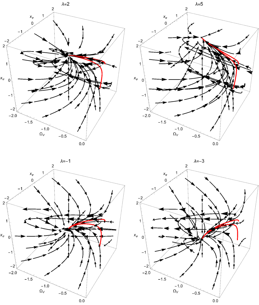
Figure 3: Phase-space portraits for the dynamical system (44) with the power-law potential. The red line corresponds to the initial conditions presented in Figs. 1 and 2.

VI Conclusions

In this study we examined the cosmological dynamics within the $f\left(Q\right)$ symmetric teleparallel gravity with a nonzero coupling between the matter and gravity. For the background geometry we consider an isotropic and homogeneous spatially flat FLRW geometry, while for the connection which describes the gravitational field we select it to be defined in the noncoincidence gauge. Within this consideration, dynamical degrees of freedom are introduced by the connection within the field equations, leading to a richer dynamical behaviour.

Although the gravitational theory is of fourth order, we select to work within the scalar field description, where the field equations are expressed as second-order equations with two scalar fields. One describes the dynamics of the connection and the second scalar field attributes the higher-order derivative components.

We employ the Hubble-normalization approach and we express the field equations in terms of dimensionless variables. We define an equivalent system of algebraic-differential equations and we express all the physical parameters in terms of the new variables.

We investigate the phase space of the resulting dynamical system and we explore the existence of stationary points. The stationary points identified in the phase-space analysis represent distinct cosmological regimes, each characterized by specific scalar field dynamics and energy contributions. However, their physical relevance depends critically on their stability properties. For a generic function $f\left(Q\right)$, we determined three families of stationary points, which describe de Sitter solutions where the potential term dominates, points $A$ and $D$; a matter-dominated epoch described by point $B$, and scaling solutions given by the stationary points $C$ and $E$.

For the power-law function $f\left(Q\right)\simeq Q^{\frac{\lambda}{\lambda-1}}$, that is, the power potential $V\left(\phi\right)=V_{0}\phi^{\lambda}$, we perform a detailed analysis of the stability properties of the stationary points. For this model, only the stationary points $B,$ $C$ and $D$ exist. It follows that point $D$ is an attractor which can describe the future acceleration of the universe. Point $B$ is a saddle point related to the matter-dominated epoch, while the scaling solution described by point $C$ can be related to the early inflationary epoch.

By comparing these results with the previous study angrg without the interacting term, that is $\beta=0$, we observe that point $B$ is the new stationary point which supports the matter-dominated era. Indeed, for $\beta=0$, this stationary point is not supported. Consequently, for this cosmological model, the introduction of the coupling function between the scalar field and the matter source is essential for the description of the matter epoch.

In future work we plan to investigate in detail the effects of the coupling parameters within the cosmological perturbations, as well as to examine if this cosmological model can describe the observable low-redshift expansion of the universe.

- (1) M. Hohmann, Phys. Rev. D 104, 124077 (2021)
- (2) L. Heisenberg, Physics Reports 1066, 1 (2024)
- (3) J. B. Jiménez, L. Heisenberg and T. S. Koivisto, Phys. Rev. D 98, 044048 (2018)
- (4) J. B. Jiménez, L. Heisenberg, T. S. Koivisto and S. Pekar, Phys. Rev. D 101, 103507 (2020)
- (5) S. Bahamonde, J. G. Valcarcel, L. Järv and J. Lember, JCAP 08, 082 (2022)
- (6) L. Järv, M. Rünkla, M. Saal and O. Vilson, Phys. Rev. D 97, 124025 (2018)
- (7) L. Järv and L. Pati, Phys. Rev. D 109, 064069 (2024)
- (8) H. Shabani, A. De and T.-H. Loo, Nucl. Phys. B 1017, 116965 (2025)
- (9) A. Paliathanasis, Phys. Dark Universe 43, 101388 (2024)
- (10) V. Gakis, M. Krssák, J.L. Said and E.N. Saridakis, Phys. Rev. D 101, 064024 (2020)
- (11) H. Shabani and A. De, (2025) [arXiv:2509.24562 [gr-qc]]
- (12) A. Paliathanasis, Eur. Phys. J. C 85, 822 (2025)
- (13) N. Dimakis, A. Giacomini, A. Paliathanasis and G. Panotopoulos, (2025) [arXiv:2503.14302]
- (14) A. Paliathanasis, Phys. Dark Univ. 46, 101585 (2024)
- (15) M. Hohmann, Phys. Rev. D 104 124077 (2021)
- (16) F. D’ Ambrosio, L. Heisenberg and S. Kuhn, Class. Quantum Grav. 39 025013 (2022)
- (17) L. Heisenberg, (2025) [arXiv:2509.18192]
- (18) A. Paliathanasis, N. Dimakis and T. Christodoulakis, Phys. Dark. Univ. 43, 101410 (2024)
- (19) S. Basilakos, A. Paliathanasis and E.N. Saridakis, Phys. Lett. B 868, 139658 (2025)
- (20) S. Bahamonte, K.F. Dialektopoulos, C. Escamilla-Rivera, G. Farrugia, V. Gakis, M. Hendry, M. Hohmann, J.L. Said, J. Mifsud and E. Di Valentino, Rep. Prog. Phys. 86, 026901 (2023)
- (21) R. Lazkoz, F.S.N. Lobo, M. Ortiz-Banos and V. Salzano, Phys. Rev. D 100, 104027 (2019)
- (22) F.K. Anagnostopoulos, S. Basilakos and E.N. Saridakis, Phys. Lett. B 822, 136634 (2021)
- (23) D. Mhamdi, S. Dahmani, A. Bouali, I.E. Bojaddaini and T. Ouali, Fortschritte der Physik 73, e70008 (2025)
- (24) S. Sahlu, A. de la Cruz-Dombriz and A. Abebe, MNRAS 539, 690 (2025)
- (25) C.G. Boiza, M. Petronikolou, M. Bouhmazi-Lopez and E.N. Saridakis, (2025) [arXiv:2505.18264]
- (26) A. Paliathanasis, Phys. Dark Univ. 49, 101993 (2025)
- (27) DESI Collaboration: M.A. Karim et al.(2025) [arXiv:2503.14739]
- (28) DESI Collaboration: M.A. Karim et al. (2025) [arXiv:2503.14738]
- (29) DESI Collaboration: K. Lodha et al. (2025) [arXiv:2503.14743]
- (30) D.A. Gomes, J.B. Jimenez, A.J. Cano and T.S. Koivisto, Phys. Rev. Lett. 132, 141401 (2024)
- (31) L. Heisenberg and M. Hohmann, JCAP 03, 063 (2024)
- (32) E.J. Copeland, A.R. Liddle and D. Wands, Phys. Rev. D 57, 4686 (1998)
- (33) T. Gonzales, G. Leon and I. Quiros, Class. Quantum Grav. 23, 3165 (2006)
- (34) H. Farajollahi and A. Salehi, JCAP 07, 036 (2011)
- (35) A.A. Coley, Phys. Rev. D 62, 023517 (2000)
- (36) S. Carloni, A. Troisi and P.K.S. Dunsby, Gen. Rel. Grav. 41, 1757 (2009)
- (37) A. Collinucci, M. Nielsen and T. Van Riet, Class. Quantum Grav. 22, 1269 (2005)
- (38) L. Csillag and E. Jensko, (2025) [arXiv:2505.15975]
- (39) M. van der Westhuizen, A. Abebe and E. Di Valentino, (2025) [arXiv:2509.04495]
- (40) W. Fang, H. Tu, J. Huang and C. Shu, Eur. Phys. J. C 76, 492 (2016)
- (41) N. Tamanini, Phys. Rev. D 89, 083521 (2014)
- (42) C. Kritpetch, N. Roy and N. Banerjee, Phys. Rev. D 111, 103501 (2025)
- (43) L. Amendola, D. Polarski and S. Tsujikawa, Phys. Rev. Lett. 98, 131302 (2007)
- (44) Y. Carloni and O. Luongo, EPJC 84, 519 (2024)
- (45) A. Paliathanasis, Phys. Dark Univ. 41, 101255 (2023)
- (46) H. Shabani, A. De, T.-H. Loo and E.N. Saridakis, Eur. Phys. J. C 84, 285 (2024)
- (47) G. Murtaza, A. De, Y.K. Goh and H.L. Liew, Annals Phys. 480, 170086 (2025)
- (48) G. Murtaza, A. De, A. Paliathanasis and T.-H. Loo, Class. Quantum Grav. 42, 195004 (2025)
- (49) A. Paliathanasis, Eur. Phys. J. C. 84, 125 (2024)
- (50) N. Dimakis, K.J. Duffy, A. Giacomini, A. Yu, Kamenschik, G. Leon and A. Paliathanasis, Phys. Dark Univ. 44, 101436 (2024)
- (51) L. P. Eisenhart, Non-Riemannian Geometry, American Mathematical Society, Colloquium Publications Vol. VIII, New York, (1927)
- (52) N. Dimakis, A. Paliathanasis, M. Roumeliotis and A. Paliathanasis, Phys. Rev. D 106, 043509 (2022)
- (53) I. Ayuso, M. Bouhmadi-Lopez, C.-Y. Chen, X.Y. Chew, K. Dialektopoulos and Y.-.C Ong, (2025) [arXiv:2506.03506]
- (54) G. Subramaniam, A. De, T.-H. Loo and Y.K. Goh, Fortsch. Phys. 71, 2300038 (2023)
- (55) S. Chakraborty, J. Dutta, D. Gregoris, K. Karwan and W. Khyllep, JCAP 05, 098 (2025)
- (56) G. Murtaza, S. Chakraborty and A. De, JCAP 08, 093 (2025)
- (57) O. Bertolami, C. Boehmer, T. Harko and F. Lobo, Phys. Rev. D 75, 104016 (2007).
- (58) O. Bertolami and J. Paramos, Class. Quantum Grav. 25, 245017 (2008)
- (59) Z. Haghani and T. Harko, Eur. Phys. J C 81, 615 (2021)
- (60) V. Gakis, M. Krššák, J.L. Said and E.N. Saridakis, Phys. Rev. D 101, 064024 (2020)
- (61) D. Zhao, Phys. Rev. D 110, 124034 (2024)
- (62) A. Paliathanasis, Gen. Rel. Grav. 55, 130 (2023)