The uniqueness of inverse scattering problems, reciprocity principles, and nonradiating sources related to low-signature structures

Abstract

This paper is about perfectly electrically conducting structures designed to produce negligible scattered power when exposed to a time-harmonic plane electromagnetic wave. The structures feature cavities capable of concealing objects. Theoretical investigations of the properties of the structures combined with accurate numerical computations lead to three key findings: the first concerns the uniqueness of the solution to an inverse scattering problem, the second establishes a reciprocity relation for the far-field scattering amplitude, and the third reveals the existence of non-radiating sources that generate substantial electromagnetic fields near the source region. The results have applications in low-observable technology.

1 Introduction

A general physical object can be considered invisible to a given incident electromagnetic wave if it is undetectable by a sensor from any direction or distance. Much of the recent research on invisibility has been focused on cloaking, as described in papers such as [6, 19]. Cloaking involves covering an object with a cloak that guides incident waves around the object without producing a scattered wave. The search for suitable materials for cloaking has led to extensive research in the area of metamaterials [5]. In microwave applications, such materials exhibit properties not found in nature. Despite progress, significant breakthroughs are still needed before cloaking can become a practical technology.

A technology related to cloaking is stealth, also known as low-observable technology. Its main goal is to minimize the detectability of military structures such as aircraft, ships, and submarines across various detection methods, including radar, infrared sensors, and sonar. In radar applications, stealth techniques aim to reduce the backscattering cross section, also known as the radar cross section (RCS) [1, Sec. 3.1], of a structure, thereby making it less visible to monostatic radar systems. This is achieved through clever designs and the use of radar-absorbing materials [1]. A structure with a small RCS is often described as having a low radar signature. The term low-signature structure, as used in this paper, refers to a structure that produces minimal scattered power in response to an incident wave. This indicates that its total scattering cross section, rather than just the RCS, is small.

This paper presents low-signature perfectly electrically conducting (PEC) structures. As in many stealth applications the structures can be fabricated from ordinary metals. They also function as cloaking devices, featuring one or several cavities that can hide objects. However, the designs of our structures differ from those used in stealth and cloaking technologies. The cavities are located between two horizontal infinitely thin PEC walls. When such a PEC structure is illuminated by a time-harmonic linearly polarized electromagnetic plane wave, the horizontal PEC walls enable the wave to pass by the cavity, essentially without producing a scattered wave. Disadvantages with our structures are that they need to be long in one spatial direction and that the incident wave must be a transverse magnetic (TM) wave with its magnetic field parallel to the horizontal walls. The advantages are that the invisibility is far better than what can be achieved by electromagnetic cloaking and that not only very low RCS is achieved but also very low total scattering cross section.

A low-signature PEC structure, similar to the ones described in this paper, is presented in [18]. Its main purpose is to reduce the signature of a cylindrical object by guiding incident waves around it. In [18], this low-signature effect is achieved only when the incident wave is a transverse electric (TE) wave, with the electric field aligned parallel to the cylinder.

The first part of this paper deals with the design of the PEC structures that can hide objects and have a low signature to an incident TM plane wave in a wide or a narrow frequency band. Three fundamental and unexpected findings are then presented regarding low-signature structures.

The first finding concerns the non-uniqueness of the inverse scattering problem for determining the boundary of PEC structures based on measured scattering data.

The second finding, derived from the Lorentz reciprocity theorem, states the following: suppose a structure is undetectable from any direction or distance when illuminated by a TM plane wave traveling, for example, in the positive $x$-direction. Then, place a sensor either in the positive or negative $x$-direction, at a large distance from the structure, and illuminate the structure by an arbitrary TM wave generated by sources located anywhere outside the structure. Then the sensor cannot detect the structure.

The third finding highlights the existence of nonradiating sources that produce a significant electromagnetic field in a vicinity of the source region.

All three findings emanate from physical assumptions and are supported by numerical computations of scattered fields and scattering cross sections. The computations are made using an integral equation method [11], which offers the numerical precision necessary to validate the findings. The numerical computations are made on broadband low-signature structures and also on the narrowband low-signature structures that were originally introduced in [12] and [13].

The rest of the paper is organized as follows. Section 2 presents the partial differential equations and boundary conditions for the TM direct scattering problem. Section 3 introduces the low-signature PEC structures. The three findings of low-signature structures are presented in Section 4. Concluding remarks are made in Section 5. A few notes on the numerical scheme [11] are collected in Appendix A.

2 The direct scattering problem

The geometric cross sections of a broadband low-signature structure and a narrowband low-signature structure are shown in Figures 1 and 2. Both structures are translational invariant and have infinite extent along the $z$-direction. Here $\Gamma_{\rm hw}$, $\Gamma_{\rm fc}$, and $\Gamma_{\rm ec}$ denote the boundaries of horizontal walls, fusiform cavities, and half-ellipse-shaped cavities, respectively. The boundaries are all PEC. Throughout the paper, the notation $\Gamma$ is used to represent the union $\Gamma_{\rm hw}\cup\Gamma_{\rm fc}$ and the union $\Gamma_{\rm hw}\cup\Gamma_{\rm ec}$. The domain exterior to $\Gamma$, denoted $\Omega$, contains air with relative permittivity $\varepsilon_{\rm r}=1$. The domain exterior to the smallest rectangle that circumscribes a given structure is denoted $\Omega_{\rm rec}$. The horizontal walls are infinitely thin. The domain enclosed by $\Gamma_{\rm fc}$ and the domains enclosed by $\Gamma_{\rm ec}$ are cavities where objects can be hidden.

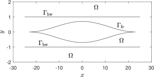
Figure 1: The geometric cross section of a broadband low-signature structure with a fusiform cavity with two cusps. The geometry is specified in (11). For the unit of length, see Remark 1.

Figure 2: The geometric cross section of a narrowband low-signature structure. The cavities are half ellipses with major axis $w$, minor axis $w/2$, and form a finite-periodic pattern with period $d$. The horizontal walls are specified in (12). For the unit of length, see Remark 1.

The structures are illuminated by a time-harmonic TM wave with angular frequency $\omega$ and complex magnetic field ${\boldsymbol{H}}^{\rm in}({\boldsymbol{\rho}})=H^{\rm in}({\boldsymbol{\rho}})\hat{{\boldsymbol{z}}}$, where ${\boldsymbol{\rho}}=x\hat{{\boldsymbol{x}}}+y\hat{{\boldsymbol{y}}}$, and $\hat{{\boldsymbol{x}}}$, $\hat{{\boldsymbol{y}}}$, and $\hat{{\boldsymbol{z}}}$ are the unit vectors in a cartesian coordinate system. The transformation to the time domain is ${\boldsymbol{H}}({\boldsymbol{\rho}},t)=\Re\{{\boldsymbol{H}}({\boldsymbol{\rho}})e^{-{\rm i}\omega t}\}$. The total magnetic field ${\boldsymbol{H}}({\boldsymbol{\rho}})=H({\boldsymbol{\rho}})\hat{{\boldsymbol{z}}}$ is the sum of the incident and the scattered field

$$H({\boldsymbol{\rho}})=H^{\rm in}({\boldsymbol{\rho}})+H^{\rm sc}({\boldsymbol{\rho}}),\quad{\boldsymbol{\rho}}\in\Omega.$$ (1)

The direct scattering problem is the exterior Neumann problem for $H^{\rm sc}({\boldsymbol{\rho}})$

$$(\nabla^{2}+k^{2})H^{\rm sc}({\boldsymbol{\rho}})=0,\quad{\boldsymbol{\rho}}\in\Omega,$$ (2)

$$\nu\cdot\nabla H^{\rm sc}({\boldsymbol{\rho}})=-\nu\cdot\nabla H^{\rm in}({\boldsymbol{\rho}}),\quad{\boldsymbol{\rho}}\in\Gamma,$$ (3)

$$H^{\rm sc}({\boldsymbol{\rho}})\to\dfrac{e^{{\rm i}k\rho}}{\sqrt{\rho}}(F^{\rm sc}(\theta)+{\mathcal{O}}(\rho^{-1})),\quad\rho\to\infty.$$ (4)

Here, $k=\omega/c_{0}$ is the wavenumber, where $c_{0}$ is the speed of light in vacuum, $\nu$ is the normal unit vector to $\Gamma$, $\rho=|{\boldsymbol{\rho}}|$, and $F^{\rm sc}(\theta)$ is the far-field amplitude of the scattered field. The angle $\theta$ is the azimuthal angle, measured from the $x$-axis.

The time average of the radiated power per unit length from a structure is

$$P=\eta_{0}\int\limits_{-\pi}^{\pi}|F^{\rm sc}(\theta)|^{2}\,{\rm d}\theta,$$ (5)

where $\eta_{0}=\sqrt{\mu_{0}/\varepsilon_{0}}$ is the wave impedance. When the incident field is a plane wave, the (total) scattering cross section is defined as

$$\Sigma=\dfrac{\text{time average of scattered power per unit length}}{\text{time average of incident power density}}.$$ (6)

An incident TM plane wave has magnetic and electric fields

$$\begin{split}&{\boldsymbol{H}}^{\rm in}({\boldsymbol{\rho}})=e^{{\rm i}{\boldsymbol{k}}\cdot{\boldsymbol{\rho}}}\hat{{\boldsymbol{z}}},\\ &{\boldsymbol{E}}^{\rm in}({\boldsymbol{\rho}})=\eta_{0}e^{{\rm i}{\boldsymbol{k}}\cdot{\boldsymbol{\rho}}}\hat{{\boldsymbol{z}}}\times\hat{{\boldsymbol{k}}},\end{split}$$ (7)

where ${\boldsymbol{k}}=k\hat{{\boldsymbol{k}}}$ is the wave vector. The angle of incidence is denoted $\alpha$ so that

$$\hat{{\boldsymbol{k}}}=(\cos\alpha,\sin\alpha,0).$$ (8)

With incident field (7) then

$$\Sigma=\eta_{0}^{-1}P.$$ (9)

Remark 1.

The unit of length is arbitrary and is omitted in the paper. It is understood that ${\boldsymbol{\rho}}$, $k^{-1}$, and $\Sigma$ are expressed in the same unit of length and so are $x$ and $y$ in Figures 1 and 2.

3 Low-signature structures

With $\alpha=0$ in (8) then $\hat{{\boldsymbol{k}}}=\hat{{\boldsymbol{x}}}$ and (7) becomes

$$\begin{split}&{\boldsymbol{H}}^{\rm in}({\boldsymbol{\rho}})=e^{{\rm i}kx}\hat{{\boldsymbol{z}}},\\ &{\boldsymbol{E}}^{\rm in}({\boldsymbol{\rho}})=\eta_{0}e^{{\rm i}kx}\hat{{\boldsymbol{y}}}.\end{split}$$ (10)

The structures in Figures 1 and 2 are considered to have a low signature to (10) if $\Sigma$ is much less than the corresponding $\Sigma$ for the structures without the horizontal walls.

A structure consisting only of the two PEC walls is called a trivial invisible structure since the incident wave (10) then satisfies $\nu\cdot\nabla H^{\rm in}({\boldsymbol{\rho}})=0$ for ${\boldsymbol{\rho}}\in\Gamma$. Thus, (2,3,4) has the trivial solution $H^{\rm sc}({\boldsymbol{\rho}})=0$ for ${\boldsymbol{\rho}}\in\Omega$ and, by that, $\Sigma=0$ and the structure is entirely invisible to (10).

3.1 Broadband structures

In the geometric cross section $z=0$, the horizontal walls and the fusiform cavity of the example structure in Figure 1 have the parameterization ${\boldsymbol{\rho}}(s)=(x(s),y(s),0)$, where

$$\begin{split}&{\boldsymbol{\rho}}(s)=(25s,\pm 1,0),\quad s\in[-1,1],\\ &{\boldsymbol{\rho}}(s)=(23s,\pm 0.7\cos^{2}(\pi s/2),0),\quad s\in[-1,1].\end{split}$$ (11)

The low signature resulting from (10) is illustrated by the numerical computations in Figure 3. Across a broad frequency range, the fusiform cavity positioned between horizontal walls demonstrates a significantly smaller $\Sigma$ compared to the same cavity without the horizontal walls. This is quite remarkable and the reason for this low signature is as follows:

The horizontal walls function as a planar waveguide that supports the propagation of transverse electromagnetic (TEM) waves. When the fusiform cavity is situated between these walls the waveguide effectively splits into two separate guides – one above and one below the cavity. The fusiform shape allows the TEM wave to pass above and below the cavity with minimal reflection. After passing the cavity, the two waves recombine to form a TEM wave with nearly the same amplitude and phase as the incident wave.

The minimum of $\Sigma$ of the blue graph in Figure 3 is at $k=1.505395$. A small $\Sigma$ does not necessarily imply that $H^{\rm sc}({\boldsymbol{\rho}})$ remains small in the near field. However, the field image of $\log_{10}$ of $|H^{\rm sc}({\boldsymbol{\rho}})|$ in Figure 4, along with $\log_{10}$ of the estimated absolute pointwise error, clearly indicate that the scattered magnetic near field is negligible within $\Omega_{\rm rec}$. The $x$- and $y$-axes are scaled differently to provide a good field resolution between the walls.

A final numerical example demonstrating the broadband low signature is presented in Figure 5. It depicts the magnitude of $|F^{\rm sc}(\theta)|$ for $-\pi<\theta<\pi$, with the angles of incidence $\alpha=0$ and $\alpha=\pi/3$ at $k=1.505395$. One may notice that $|F^{\rm sc}(0)|$, and $|F^{\rm sc}(\pm\pi)|$ are very small when $\alpha=\pi/3$. This phenomenon is due to reciprocity and is explained in Section 4.2 below.

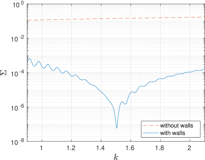
Figure 3: $\Sigma$ as a function of $k$ for the fusiform cavity in Figure 1. Dashed red line: without horizontal walls. Solid blue line: with horizontal walls. The minimum is at $k=1.505395$.

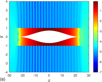
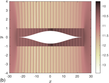
Figure 4: The structure in Figure 1 illuminated by (10) at $k=1.505395$; (a) $\log_{10}$ of $|H^{\rm sc}({\boldsymbol{\rho}})|$; (b) $\log_{10}$ of estimated absolute pointwise error in $H^{\rm sc}({\boldsymbol{\rho}})$.

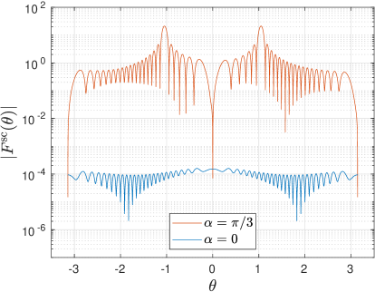
Figure 5: The structure in Figure 1 illuminated by (7) at $k=1.505395$. Red line: $\log_{10}$ of $|F^{\rm sc}(\theta)|$ at oblique incidence with $\alpha=\pi/3$; Blue line: $\log_{10}$ of $|F^{\rm sc}(\theta)|$ at perpendicular incidence ($\alpha=0$);

3.2 Narrowband structures

The example narrowband low-signature structure in Figure 2 has a finite-periodic set of six PEC half-ellipse-shaped cavities between the horizontal walls. The shape and number of cavities can vary, but they must be identical and equally spaced to achieve low signature. The low-signature property of such narrowband structures can be explained by waveguide theory [12, Sec. IIB].

The horizontal walls in Figure 2 are given by

$${\boldsymbol{\rho}}(s)=((7.3+2.5d+w/2)s,0.5\pm 0.5,0),\quad s\in[-1,1].$$ (12)

The half ellipses have period $d=2$, major axes $w$, and minor axes $w/2$, with $w=0.939225885952$. Figure 6(d) shows that $F^{\rm sc}(\theta)$ is negligible for all $\theta$ when $k=0.523371641653$ in (10). Consequently, by (6) and (5), the structure has an almost zero signature to (10) at this wavenumber. Furthermore, Figure 6 shows that the scattered magnetic near field is almost zero within $\Omega_{\rm rec}$. It should be noted, though, that the low signature is maintained only within a very narrow frequency band. Narrowband structures of the type shown in Figure 2 are mainly effective in applications where the wave frequency is precisely known.

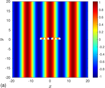
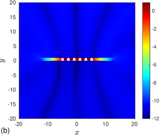
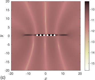
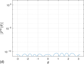
Figure 6: The plane wave (10) incident on the structure in Figure 2 with $k=0.523371641652$, and with $d=2$ and $w=0.939225885952$ in (12). (a) real part of $H({\boldsymbol{\rho}})$; (b) $\log_{10}$ of $|H^{\rm sc}({\boldsymbol{\rho}})|$; (c) $\log_{10}$ of estimated absolute pointwise error in $|H^{\rm sc}({\boldsymbol{\rho}})|$; (d) $|F^{\rm sc}(\theta)|$.

4 Features of low-signature structures

Three somewhat surprising features of low-signature structures are now presented.

4.1 The inverse scattering problem

Inverse scattering has been a highly active area of research for well over 50 years [4]. Inverse electromagnetic scattering focuses on finding the properties of an object using data collected from direct scattering experiments. The inverse scattering problem addressed here is to determine the shape of the boundary of a two-dimensional (2D) PEC structure from measured values of the scattered electric or magnetic field due to an incident TM or TE wave. If the scattered magnetic or electric fields are measured with finite sensitivity in $\Omega_{\rm rec}$, then the following holds:

The inverse scattering 2D problem of determining the shape of a PEC structure is not guaranteed to have a unique solution if the incident waves are restricted to be 2D single-frequency TM or TE waves generated by sources in $\Omega_{\rm rec}$.

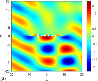
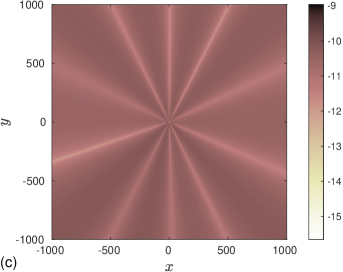
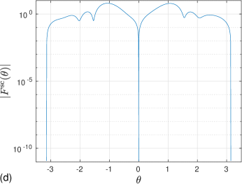
Figure 7: The plane wave (7) with $\alpha=\pi/3$ incident on the structure in Figure 2: (a) real part of $H({\boldsymbol{\rho}})$. (b) $\log_{10}$ of $|H^{\rm sc}({\boldsymbol{\rho}})|\sqrt{\rho}$; (c) $\log_{10}$ of estimated absolute pointwise error in $|H^{\rm sc}({\boldsymbol{\rho}})|\sqrt{\rho}$; (d) $|F^{\rm sc}(\theta)|$.

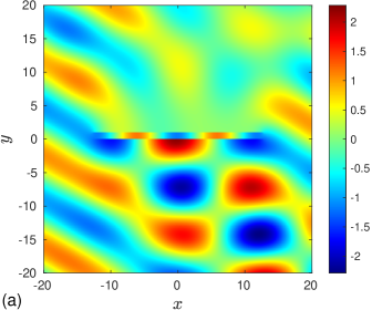
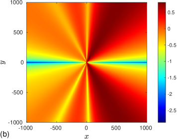
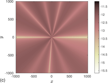
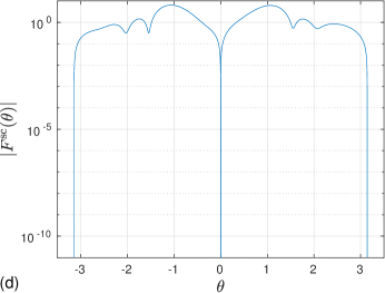
Figure 8: The plane wave (7) with $\alpha=\pi/3$ incident on the structure in Figure 2 without the half-ellipse-shaped cavities: (a) real part of $H({\boldsymbol{\rho}})$. (b) $\log_{10}$ of $|H^{\rm sc}({\boldsymbol{\rho}})|$; (c) $\log_{10}$ of estimated absolute pointwise error in $|H^{\rm sc}({\boldsymbol{\rho}})|$; (d) $|F^{\rm sc}(\theta)|$.

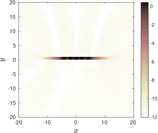
Figure 9: $\log_{10}$ of $|H_{\rm A}({\boldsymbol{\rho}})-H_{\rm B}({\boldsymbol{\rho}})|$. The real parts of $H_{\rm A}({\boldsymbol{\rho}})$ and $H_{\rm B}({\boldsymbol{\rho}})$ are shown in Figures 7(a) and 8(a), respectively.

We now confirm this statement. Let structure A be the structure in Figure 2, with $d=2$ and $w=0.939225885952$ in (12), and let structure B be the corresponding trivial structure, that is the structure with only the horizontal walls. Let $k=0.523371641653$ and the incident field be an arbitrary 2D wave generated by sources in $\Omega_{\rm rec}$. Then the two structures have the same scattered electromagnetic fields in $\Omega_{\rm rec}$. Waveguide theory provides an explanation:

First, let the incident wave be TM. For both structures, the incident wave gives rise to two TEM waves between the horizontal walls, one at the opening to the left traveling in the positive $x$-direction, and one at the opening to the right, traveling in the negative $x$-direction. The cavities in structure A are designed so that the TEM waves are transmitted between the openings in the same way as they are transmitted between the openings in structure B. Thus, the contribution by the TEM waves to $H^{\rm sc}({\boldsymbol{\rho}})$ for ${\boldsymbol{\rho}}\in\Omega_{\rm rec}$ must be the same for the two structures. The incident wave also excites the planar waveguide TM_n modes with $n>0$ [12, Eq. (11)] at the openings, but these modes attenuate fast and have a negligible amplitude at the cavities.

Next, let the incident wave be TE. At the openings it can only excite the planar waveguide TE_n modes with $n>0$ and at $k=0.523371641653$ they attenuate fast enough to have a negligible amplitude at the cavities. Thus the scattered fields in $\Omega_{\rm rec}$ are not affected by the cavities and by that the scattered fields from structure A is the same as those from structure B.

To further verify the statement we present two numerical examples, one with an incident TM wave and one with an incident TE wave.

Let the incident wave be (7) with $k=0.523371641653$, and $\alpha=\pi/3$ in (8). The resulting field images of the real part of $H({\boldsymbol{\rho}})$ are shown in Figure 7(a) for structure A and in Figure 8(a) for structure B. In $\Omega_{\rm rec}$ the field image of Figure 7(a) is indistinguishable from the image of Figure 8(a). The similarity is confirmed by Figure 9 which shows $|H_{\sf A}({\boldsymbol{\rho}})-H_{\sf B}({\boldsymbol{\rho}})|$ in the square $-20<x,y<20$. In the part of the square belonging to $\Omega_{\rm rec}$ the difference is less than $10^{-9}$.

Next, let the incident wave be the TE wave

$$\begin{split}&{\boldsymbol{H}}^{\rm in}({\boldsymbol{\rho}})=e^{{\rm i}{\boldsymbol{k}}\cdot{\boldsymbol{\rho}}}\hat{{\boldsymbol{k}}}\times\hat{{\boldsymbol{z}}},\\ &{\boldsymbol{E}}^{\rm in}({\boldsymbol{\rho}})=\eta_{0}e^{{\rm i}{\boldsymbol{k}}\cdot{\boldsymbol{\rho}}}\hat{{\boldsymbol{z}}}.\end{split}$$ (13)

The structures A and B, the angle of incidence $\alpha$, and the wavenumber $k$ remain unchanged from those used for the TM wave above. The difference $|E_{\sf A}({\boldsymbol{\rho}})-E_{\sf B}({\boldsymbol{\rho}})|$ is shown in Figure 10. Note that TE waves are polarized such that ${\boldsymbol{E}}({\boldsymbol{\rho}})=E({\boldsymbol{\rho}})\hat{{\boldsymbol{z}}}$, where $E({\boldsymbol{\rho}})$ satisfies the exterior Dirichlet problem. This problem is given by (1,2,4), with $H$ replaced by $E$, and the boundary condition $E^{\rm sc}({\boldsymbol{\rho}})=-E^{\rm in}({\boldsymbol{\rho}})$ for ${\boldsymbol{\rho}}\in\Gamma$.

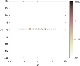
Figure 10: $\log_{10}$ of $|E_{\rm A}({\boldsymbol{\rho}})-E_{\rm B}({\boldsymbol{\rho}})|$ for the TE wave (13) with $\alpha=\pi/3$ and $k=0.523371641653$ incident on the structure A and B, where A is the structure in Figure 2 with cavities and B is the same structure without cavities.

Figures 9 and 10 show that $|H_{\sf A}({\boldsymbol{\rho}})-H_{\sf B}({\boldsymbol{\rho}})|\approx 0$ and $|E_{\sf A}({\boldsymbol{\rho}})-E_{\sf B}({\boldsymbol{\rho}})|\approx 0$ for ${\boldsymbol{\rho}}\in\Omega_{\rm rec}$. This means that the inverse problem of reconstructing the boundary of a PEC structure from experimental data, obtained with plane waves at a single wavenumber, is not necessarily uniquely solvable. This conclusion applies not only to incident plane waves, but to any 2D TM or TE incident wave with sources located in $\Omega_{\rm rec}$.

4.2 Reciprocity applied to invisible structures

Consider a structure similar to the one in Figure 2 that is invisible to (10) at a wavenumber $k=k_{\rm inv}$. Using the Lorentz reciprocity theorem, [15, Sec. 1.3.5], one can prove that $F^{\rm sc}(0)\approx 0$ and $F^{\rm sc}(\pi)\approx 0$ when $k=k_{\rm inv}$ and the incident wave is an arbitrary TM wave generated by a source in $\Omega_{\rm rec}$.

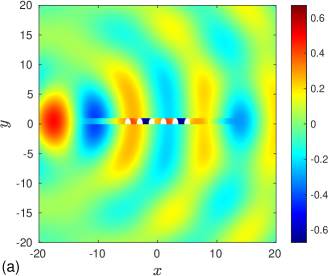
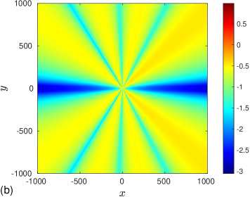
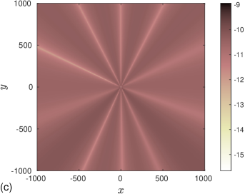
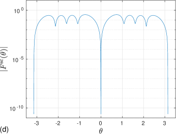
Figure 11: Field images for the structure in Figure 2 with incident field (14), ${\boldsymbol{\rho}}_{0}=(-14,0.5,0)$, and $k=0.523371641653$: (a) real part of $H({\boldsymbol{\rho}})$; (b) $\log_{10}$ of $|H^{\rm sc}({\boldsymbol{\rho}})|\sqrt{\rho}$; (c) $\log_{10}$ of estimated absolute pointwise error in $|H^{\rm sc}({\boldsymbol{\rho}})|\sqrt{\rho}$; (d) $|F^{\rm sc}(\theta)|$.

4.2.1 Numerical examples for reciprocity

Figures 7(d) and 8(d) show that, in accordance with reciprocity, $F^{\rm sc}(0)\approx 0$ and $F^{\rm sc}(\pi)\approx 0$ for (7) with $\alpha=\pi/3$. The reciprocity is also confirmed in Figure 5 where $F^{\rm sc}(0)$ and $F^{\rm sc}(\pm\pi)$ are very small for the broadband structure when $\alpha=\pi/3$ and $k=1.505395$.

As a final verification of reciprocity, we consider the incident wave generated by a 2D electric dipole with its current directed along $\hat{{\boldsymbol{y}}}$. The incident magnetic field from this dipole is

$${\boldsymbol{H}}^{\rm in}({\boldsymbol{\rho}})=-\sqrt{\dfrac{\pi k}{2}}\dfrac{({\boldsymbol{\rho}}-{\boldsymbol{\rho}}_{0})\times\hat{{\boldsymbol{y}}}}{|{\boldsymbol{\rho}}-{\boldsymbol{\rho}}_{0}|}H_{1}^{(1)}(k|{\boldsymbol{\rho}}-{\boldsymbol{\rho}}_{0}|).$$ (14)

Here ${\boldsymbol{\rho}}_{0}=x_{0}\hat{{\boldsymbol{x}}}+y_{0}\hat{{\boldsymbol{y}}}$ is the position of the dipol and $H_{1}^{(1)}$ is the first order Hankel function of the first kind. The incident field (14) is normalized such that the far-field amplitude, also called the radiation pattern, of the dipole in free space is

$$|F(\theta)|=|\sin\theta|.$$ (15)

Let the structure be the same as in Figure 6, and let $k=0.523371641653$. With ${\boldsymbol{\rho}}_{0}=(-14,0.5,0)$ the real part of $H({\boldsymbol{\rho}})$, $\log_{10}$ of $|H^{\rm sc}({\boldsymbol{\rho}})|$, $\log_{10}$ of estimated absolute pointwise error in $|H^{\rm sc}({\boldsymbol{\rho}})|$, and $|F^{\rm sc}(\theta)|$ are as in Figure 11. It is clear from Figure 11(d) that $F^{\rm sc}(0)\approx 0$ and $F^{\rm sc}(\pi)\approx 0$. The singularity of the incident field at ${\boldsymbol{\rho}}={\boldsymbol{\rho}}_{0}$ is not visible in Figure 11(a) because the real part of $H_{1}^{(1)}(k|{\boldsymbol{\rho}}-{\boldsymbol{\rho}}_{0}|)$ is finite everywhere.

4.3 Nonradiating sources

In the example shown in Figure 6, the sources for $H^{\rm sc}({\boldsymbol{\rho}})$ are the surface currents on $\Gamma$. Figure 6(d) shows that the radiated power (5) from the narrowband structure is negligible at $k=0.523371641652$ since $F^{\rm sc}(\theta)\approx 0$ for all $\theta$. According to the definitions of nonradiating sources, [8, p. 275], [16, p. 1], [14, p. 2], the surface currents on $\Gamma$ thus form a nonradiating source. It is a well-established result, [7, Thm. 3.2], that the field radiated from a nonradiating 3D source is zero everywhere outside a sphere circumscribing the source. The theorem also applies in two dimensions if the sphere is replaced by a circle. This is in accordance with Figure 6(b,d). Under certain restrictions it can be shown using Rellich’s lemma, originally proven in [17], that the radiated field of a nonradiating source is zero outside the source region [8, Thm. 2.3], [4, Lem. 1], [2, p. 3824], [14, Eq. (3.4a)], [20, Thm. 1]. In contrast, Figure 6(b) shows that $H^{\rm sc}({\boldsymbol{\rho}})$ is quite large between the walls but outside the source region. This raises questions about the validity of applying Rellich’s lemma to the nonradiating sources that are induced by an incident wave.

5 Conclusions

It is evident that an infinitely thin horizontal PEC wall is entirely invisible to the incident wave (10). This fundamental property gives rise to some rather surprising results discussed in this paper. One key outcome is that it is possible to design low-signature PEC structures composed of two horizontal PEC walls, with either a PEC fusiform cavity or a finite-periodic array of PEC cavities positioned between them. Within these cavities, objects can be concealed from an incident plane wave, effectively making the low-signature PEC structures act as invisibility cloaks.

In addition to presenting the low-signature structures, the paper highlights three main findings. First, the inverse problem of determining the shape of a PEC surface does not necessarily have a unique solution when only single-frequency incident waves are used. Second, based on reciprocity, the far-field amplitude $F^{\rm sc}(\theta)$ satisfies $F^{\rm sc}(0)\approx 0$ and $F^{\rm sc}(\pi)\approx 0$ when the low-signature structures are illuminated by any TM wave generated within $\Omega_{\rm rec}$. Third, it is demonstrated that non-radiating sources can produce significant electromagnetic fields near the source location, which contradicts an established opinion regarding non-radiating sources.

Acknowledgments

This work was supported by the Swedish Research Council under contract 2021-03720.

Appendix

Appendix A Notes on the numerical scheme

In [11], a boundary integral equation (BIE) based numerical scheme is presented for solving the exterior Neumann problem (2,3,4) and the corresponding exterior Dirichlet problem. This scheme applies to structures with boundaries $\Gamma$ being collections of open arcs, such as those shown in Figures 1 and 2. It is used for all computations in the present paper. In the context of (2,3,4) it contains steps such as: choosing a layer-potential field representation for $H^{\rm sc}({\boldsymbol{\rho}})$; rewriting (2,3,4) as a BIE based on that representation; Nyström discretization of the BIE on a graded mesh, accelerated and stabilized with recursively compressed inverse preconditioning (RCIP) [10]; and iterative solution of large linear systems using the generalized minimal residual method (GMRES), accelerated with the fast multipole method (FMM) [9].

We shall not review much detail of the scheme in [11] here, but chiefly mention that, for the exterior Neumann problem, it prescribes the choice of field representation

$$H^{\rm sc}({\boldsymbol{\rho}})=-2\int_{\Gamma}\frac{\partial\Phi_{k}}{\partial\nu^{\prime}}({\boldsymbol{\rho}},{\boldsymbol{\rho}}^{\prime})S_{k}\varrho({\boldsymbol{\rho}}^{\prime})\,{\rm d}\ell^{\prime}\,,\quad{\boldsymbol{\rho}}\in\Omega\,.$$ (16)

Here $\varrho({\boldsymbol{\rho}})$ is a layer density on $\Gamma$ to be determined, $\Phi_{k}({\boldsymbol{\rho}},{\boldsymbol{\rho}}^{\prime})$ is the fundamental solution to the Helmholtz equation in the plane [3, Eq. (3.60)], $S_{k}$ is the single-layer operator [3, Eq. (3.8)], ${\rm d}\ell$ is an element of arc length, and $\partial/\partial\nu^{\prime}=\nu({\boldsymbol{\rho}}^{\prime})\cdot\nabla^{\prime}$. Insertion of (16) into (3) gives the BIE with composed integral operators

$$T_{k}(-S_{k})\varrho({\boldsymbol{\rho}})=-\nu\cdot\nabla H^{\rm in}({\boldsymbol{\rho}})\,,\quad{\boldsymbol{\rho}}\in\Gamma\,,$$ (17)

which is [11, Eq. (31)] and where $T_{k}$ is the hypersingular operator [3, Eq. (3.11)].

While the scheme in [11] with (16) is generally applicable to exterior Neumann problems, in the present paper we only use (16) for $\Gamma$ as in Figure 2. For $\Gamma$ as in Figure 1, we take advantage of that $\Gamma_{\rm fc}$ is a closed contour, rather than a general collection of open arcs, and replace (16) with

$$H^{\rm sc}({\boldsymbol{\rho}})=-2\int_{\Gamma_{\rm hw}}\frac{\partial\Phi_{k}}{\partial\nu^{\prime}}({\boldsymbol{\rho}},{\boldsymbol{\rho}}^{\prime})S_{k}\varrho({\boldsymbol{\rho}}^{\prime})\,{\rm d}\ell^{\prime}\\ -2\int_{\Gamma_{\rm fc}}\Phi_{k}({\boldsymbol{\rho}},{\boldsymbol{\rho}}^{\prime})\varrho({\boldsymbol{\rho}}^{\prime})\,{\rm d}\ell^{\prime}\,,\quad{\boldsymbol{\rho}}\in\Omega\cup\Gamma_{\rm fc}\,,$$ (18)

which is simpler than (16). Insertion of (18) into (3) gives a BIE, analogous to (17), which in composed block operator form can be written

$$\begin{bmatrix}T_{k}^{\rm(hw,hw)}&-K_{k}^{\rm A(hw,fc)}\\ T_{k}^{\rm(fc,hw)}&I^{\rm(fc,fc)}-K_{k}^{\rm A(fc,fc)}\end{bmatrix}\begin{bmatrix}-S_{k}^{\rm(hw,hw)}&0\\ 0&I^{\rm(fc,fc)}\end{bmatrix}\begin{bmatrix}\varrho_{\rm hw}({\boldsymbol{\rho}})\\ \varrho_{\rm fc}({\boldsymbol{\rho}})\end{bmatrix}=\begin{bmatrix}g_{\rm hw}({\boldsymbol{\rho}})\\ g_{\rm fc}({\boldsymbol{\rho}})\end{bmatrix}.$$ (19)

Here $I^{(i,j)}$, $S_{k}^{(i,j)}$, $K_{k}^{{\rm A}(i,j)}$, $T_{k}^{(i,j)}$ are operators acting on densities at $\Gamma_{j}$ and evaluated at $\Gamma_{i}$ with $i,j={\rm hw,fc}$. Furthermore, $I$ is the identity operator, $K_{k}^{\rm A}$ is the adjoint double-layer operator [3, Eq. (3.10)], and $\varrho_{\rm hw}({\boldsymbol{\rho}})$, $\varrho_{\rm fc}({\boldsymbol{\rho}})$, $g_{\rm hw}({\boldsymbol{\rho}})$, $g_{\rm fc}({\boldsymbol{\rho}})$ are the restrictions of $\varrho({\boldsymbol{\rho}})$ and of $-\nu\cdot\nabla H^{\rm in}({\boldsymbol{\rho}})$ to $\Gamma_{\rm hw}$ and to $\Gamma_{\rm fc}$, respectively.

We emphasize that the machinery for applying RCIP to (17), described in [11], also applies to (19) and that the subsequent computational steps of the scheme are the same regardless of whether (16) and (17) or (18) and (19) are chosen.

References

- [1] H. Ahmad, et al., “Stealth technology: Methods and composite materials: A review,” Polymer Composites 40(12), 4457–4472, 2019.
- [2] E. Blåsten and H. Liu, “Scattering by curvatures, radiationless sources, transmission eigenfunctions, and inverse scattering problems,” SIAM Journal on Mathematical Analysis, 53(4), 3801–3837, 2021.
- [3] D. Colton and R. Kress, Inverse acoustic and electromagnetic scattering theory, Applied Mathematical Sciences vol. 93, 2nd ed., Springer-Verlag, Berlin, 1998.
- [4] D. Colton and R. Kress, “Looking back on inverse scattering theory,” SIAM Review 60, 779–807, 2018.
- [5] J. Fan, L. Zhang, S. Wei, Z. Zhang, S. K. Choi, B. Song, and Y. Shi, “A review of additive manufacturing of metamaterials and developing trends,” Materials Today, 50, 303–328, 2021.
- [6] R. Fleury, F. Monticone, and A. Alù, “Invisibility and cloaking: Origins, present, and future perspectives,” Physical Review Applied, 4(3), article no. 037001, 2015.
- [7] F. Friedlander, “An inverse problem for radiation fields,” Proceedings of the London Mathematical Society 2, 551–576, 1973.
- [8] G. Gbur, “Nonradiating sources and other ’invisible’ objects,” In E.Wolf (Ed.), Progress in optics, Amsterdam: Elsevier, 45, 273–315, 2003.
- [9] Z. Gimbutas, L. Greengard, M. O’Neil, M. Rachh, and V. Rokhlin. fmm2d software library, https://github.com/flatironinstitute/fmm2d. Accessed: October 18, 2024.
- [10] J. Helsing. “Solving integral equations on piecewise smooth boundaries using the RCIP method: a tutorial,” arXiv e-prints, arXiv:1207.6737v10 [physics.comp-ph], revised 2022.
- [11] J. Helsing and S. Jiang, “The Helmholtz Dirichlet and Neumann problems on piecewise smooth open curves,” Journal of Computational Physics, 539, article no. 114223, 2025.
- [12] J. Helsing, S. Jiang, and A. Karlsson, “Design of perfectly conducting objects that are invisible to an incident plane wave,” IEEE Journal on Multiscale and Multiphysics Computational Techniques, 9, 104–112, 2024.
- [13] J. Helsing, S. Jiang, and A. Karlsson, “Designing objects that are invisible to electromagnetic waves,” American Journal of Physics, 93(6), 459–466, 2025.
- [14] K. Kim and E. Wolf, “Non-radiating monochromatic sources and their fields,” Optics communications, 59(1), 1–6, 1986.
- [15] G. Kristensson, Scattering of electromagnetic waves by obstacles, Mario Boella Series on Electromagnetism in Information and Communication, SciTech Publishing, an imprint of the IET, Edison, NJ, 2016.
- [16] P. Li and J. Wang, “Nonradiating sources of Maxwell’s equations,” arXiv e-prints, arXiv:2402.10407 [math.AP], 2024.
- [17] F. Rellich, “Über das asymptotische Verhalten der Lösungen von im unendlichen Gebieten,” Jahresbericht der Deutschen Mathematiker-Vereinigung, 53, 57–65, 1943.
- [18] S. Tretyakov, P. Alitalo, O. Luukkonen, and C. Simovski, “Broadband electromagnetic cloaking of long cylindrical objects,” Physical Review Letters, 103(10), article no. 103905, 2009.
- [19] F. Vasquez, G. Milton, and D. Onofrei, “Active exterior cloaking for the 2D Laplace and Helmholtz equations,” Physical Review Letters 103(7), article no. 073901, 2009.
- [20] E. Vesalainen, “Rellich type theorems for unbounded domains,” arXiv e-prints, arXiv:1401.4531 [math.AP], 2014.