A robust computational framework for the mixture-energy-consistent six-equation two-phase model with instantaneous mechanical relaxation terms

Abstract

We present a robust computational framework for the numerical solution of a hyperbolic 6-equation single-velocity two-phase model. The model’s main interest is that, when combined with instantaneous mechanical relaxation, it recovers the solution of the 5-equation model of Kapila. Several numerical methods based on this strategy have been developed over the years. However, neither the 5- nor 6-equation model admits a complete set of jump conditions because they involve non-conservative products. Different discretizations of these terms in the 6-equation model exist. The precise impact of these discretizations on the numerical solutions of the 5-equation model, in particular for shocks, is still an open question to which this work provides new insights. We consider the phasic total energies as prognostic variables to naturally enforce discrete conservation of total energy and compare the accuracy and robustness of different discretizations for the hyperbolic operator. Namely, we discuss the construction of an HLLC approximate Riemann solver in relation to jump conditions. We then compare an HLLC wave-propagation scheme which includes the non-conservative terms, with Rusanov and HLLC solvers for the conservative part in combination with suitable approaches for the non-conservative terms. We show that some approaches for the discretization of non-conservative terms fit within the framework of path-conservative schemes for hyperbolic problems. We then analyze the use of various numerical strategies on several relevant test cases, showing both the impact of the theoretical shortcomings of the models as well as the importance of the choice of a robust framework for the global numerical strategy.

⁽¹⁾ CMAP, CNRS, École polytechnique, Institut Polytechnique de Paris
Route de Saclay, 91120 Palaiseau, France
giuseppe.orlando@polytechnique.edu, ward.haegeman@polytechnique.edu, marc.massot@polytechnique.edu

⁽²⁾ Department of Multi-Physics for Energetics, ONERA, Université Paris-Saclay
F-91123 Palaiseau, France

⁽³⁾ IMSIA, UMR 9219 ENSTA-CNRS-EDF,
ENSTA Paris, Institut Polytechnique de Paris,
91120 Palaiseau, France
marica.pelanti@ensta.fr

Keywords: Two-phase flows, 6-equation model, Finite Volume schemes, Wave-propagation scheme, Non-conservative terms discretization, Riemann solvers, Relaxation source terms.

1 Introduction

Two-phase flows are relevant in several areas of engineering, such as naval engineering or aerospace engineering, and are characterized by the simultaneous presence of two phases with different properties. A widely established model for compressible two-phase flows is the full non-equilibrium 7-equation Baer-Nunziato (BN) model [7], originally proposed for detonation waves in granular explosives, and then extended to liquid-gas flows in [58]. The model assumes that each phase is compressible and evolves with its own pressure, temperature, and velocity, together with an evolution equation for the volume fraction of one of the two phases. Taking into account the compressibility of both phases is fundamental to correctly capture wave-propagation phenomena and acoustic perturbations, and it is crucial in the case of liquid-vapour transition [59].

Reduced models have been derived by means of asymptotic expansions of the BN model with assumptions of infinitely fast relaxation towards the equilibrium for the velocity, pressure or temperature, see, e.g., [38, 50]. Among them, a widely employed model is the 5-equation single-velocity single-pressure model, also known as Kapila model [38]. The main difficulty in the design of robust numerical schemes for the 5-equation model stems from the non-conservative term in the volume fraction equation that depends on the divergence of the flow velocity and on the phasic compressibilities [51, 60]. The variation of the volume fraction across shock waves associated with this term makes the construction of approximate Riemann solvers more challenging with respect to the 6-equation model. Moreover, the presence of this non-conservative term in the equation of the volume fraction makes difficult to preserve the bounds of the volume fraction when dealing with shocks and strong rarefaction waves [60].

Alternative strategies for the numerical solution of the 5-equation model have been proposed in the literature relying on the relaxation of non-equilibrium models. Following the derivation performed at the continuous level, one could start from the numerical solution of the BN model and then perform instantaneous velocity and pressure relaxations. The BN model is also characterized by non-conservative terms, but, under specific choices of the interfacial pressure and velocity, it is well posed, in the sense that non-conservative products are uniquely defined and the model admits a mixture entropy inequality to select physically relevant weak solutions [30]. Its numerical solution is rather challenging, even though numerical methods which are positivity-preserving and entropy-consistent are nowadays available [18, 57]. However, the wave structure of the BN model is definitely more complex than that of the reduced Kapila model, as it exhibits a larger number of acoustic waves and involves multiple velocities [66].

An alternative and popular strategy consists in resolving the 6-equation single-velocity model with instantaneous mechanical relaxation [51, 52, 60]. This model assumes velocity equilibrium between the two phases, keeping mechanical, thermal, and chemical non-equilibrium effects. More specifically, we consider here the 6-equation single-velocity model as presented in [51]. Hence, the model consists of an advection equation for the volume fraction of one phase, together with the continuity equation and the total energy balance of each phase, and a mixture momentum equation. Alternative formulations of the 6-equation model have been proposed in the literature using the equations of the phasic internal energies instead of those of the total energies, see [60, 72]. However, as discussed in [51], while the two systems are mathematically equivalent for smooth solutions, the use of phasic total energies provides several advantages in terms of numerical robustness. In particular, it ensures automatically conservation of the mixture total energy. Formulations based on phasic internal energies require instead the use of an additional conservation law to correct the thermodynamic state and to guarantee the conservation of the total energy [60, 62, 72]. The main advantage of relaxing the 6-equation model instead of the 7-equation model is that its wave structure is similar to that of the 5-equation model. However, the 6-equation model contains non-conservative terms for which, unlike the BN model, a complete set of jump conditions cannot be uniquely defined, making the design of Riemann solvers and the choice of suitable numerical methods challenging. The choice of starting from the 7- or 6-equation model reflects the trade-off between the good mathematical properties of the 7-equation model and the simpler wave structure of the 6-equation model and its reduced number of equations, in particular for multi-dimensional computations. In this work, we focus on the latter of these two strategies.

The aim of the present paper is to provide a quantitative comparison among different numerical discretization strategies for the aforementioned 6-equation model so as to identify a robust computational framework that can be employed in combination with the instantaneous mechanical relaxation. In most standard contributions [51, 60, 61], the 6-equation model has been employed only as an auxiliary tool to solve the 5-equation model, thus combining its numerical solution with the instantaneous mechanical relaxation. However, the accurate and robust numerical solution of the 6-equation model is a crucial step and it is therefore important to assess the properties of the numerical method employed to solve the 6-equation model. Furthermore, some recent contributions equipped the 6-equation model with finite-rate mechanical relaxation [50, 62]. When doing so, the model is no longer an auxiliary system used for the numerical resolution of the Kapila model, but acquires the status of a standalone model, thus understanding its discretization is even more important and this is one of the goals of the present work.

The spatial discretization is based on the finite volume (FV) method as implemented in the framework of samurai and approximate Riemann solvers, such as the Rusanov flux [56] and the HLLC [42], are employed. Several numerical methods for the 6-equation model have been developed over the years, see, among many others [22, 51, 52, 60] and the references therein. In this work, we compare in terms of robustness and accuracy two numerical strategies; in the first one, we employ the approximate Riemann solver for the conservative part in combination with suitable approaches for the non-conservative terms [8, 19, 46, 68], whereas in the second one we adopt the so-called wave-propagation method as described in [42]. This second approach has been employed for the solution of the 6-equation model with instantaneous mechanical relaxation in [50, 51].

Instantaneous mechanical relaxation may be applied after each hyperbolic step. We have already mentioned the advantages in resolving the 6-equation model with respect to the 5-equation model. However, we show here that, while for most test cases all numerical schemes yield virtually identical results for the 5-equation model, under extreme conditions, different numerical schemes converge to different solutions. Since jump conditions are not uniquely defined, different discretization techniques of the hyperbolic operator, in particular the non-conservative products, may lead to different partitions of the phasic energies and ultimately lead to different shock profiles, even though global conservation is ensured. The analysis of the discretization strategies for the 6-equation model carried out in this contribution is complementary to a recent work of two of the authors in which a complete analysis of the pressure relaxation operator is provided [33]. In their work, it has been shown how, for a given spatial discretization of the 6-equation model, the choice of the pressure relaxation operator may impact the numerical results. In particular, the interfacial pressure plays a role only in the relaxation process and does not appear in the 5-equation model. The choice of the interfacial pressure in the relaxation process, as well as the relaxation techniques, may impact the robustness of the numerical strategy or affect the computed shock profiles. The impact of the spatial discretization scheme for the hyperbolic operator of the 6-equation model was not part of the study presented in [33]. This is what the present work focuses on as we consider various treatments for the spatial discretization of the non-conservative products present in the model and consider only a single relaxation strategy. Combined, the present contribution and the one in [33], aim at providing a complete and in-depth analysis of the overall numerical strategy. In conclusion, the goal of the paper is to show a robust computational framework for the solution of the 6-equation model that can then be employed in combination with the instantaneous mechanical relaxation to solve numerically the 5-equation model, limiting the impact of the shortcomings of the models. In order to achieve the goal, we present a novel analysis of the jump conditions and construction of approximate Riemann solvers as well as a novel perspective on the numerical treatment of non-conservative terms.

The paper is structured as follows. The 6-equation single-velocity two-phase model with instantaneous mechanical relaxation is presented in Section 2. The different numerical strategies for the discretization of the hyperbolic operator are reported in Section 3. Here we also briefly recall the wave-propagation method. Since the 6-equation model does not admit a complete set of jump conditions, a detailed discussion on the hypotheses employed to build the HLLC approximate Riemann solver is provided. Numerical results on a number of benchmarks to assess the robustness and the accuracy of the different approaches presented in Section 3 are reported in Section 4. Following the outcomes of these results, we show that some of the approaches employed for the discretization of non-conservative terms, originally designed for diffusion operators, can be reformulated in the framework of the well-know path conservative schemes for hyperbolic problems [48], so as to justify why certain approaches are more robust than other ones. The analysis of the instantaneous mechanical relaxation is presented in Section 6. The quantitative numerical assessment of the mechanical relaxation is presented in Section 7. Finally, some conclusions and perspectives for future work are presented in Section 8.

2 Two-phase models

In this section, the 6-equation model followed by the 5-equation model and their properties are described. Endowed with instantaneous mechanical relaxation source terms, the 6-equation model may be used as an auxiliary model for the resolution of the 5-equation model of Kapila. Using the formulation proposed in [51], the model reads as follows

$$\frac{\partial{\alpha_{1}}}{\partial{t}}+\bm{u}\cdot\operatorname{\nabla}\alpha_{1} =\mu\left(p_{1}-p_{2}\right),$$ (1a)

$$\frac{\partial{\alpha_{1}\rho_{1}}}{\partial{t}}+\operatorname{\nabla\cdot}\left(\alpha_{1}\rho_{1}\bm{u}\right) =0,$$ (1b)

$$\frac{\partial{\alpha_{2}\rho_{2}}}{\partial{t}}+\operatorname{\nabla\cdot}\left(\alpha_{2}\rho_{2}\bm{u}\right) =0,$$ (1c)

$$\frac{\partial{\rho\bm{u}}}{\partial{t}}+\operatorname{\nabla\cdot}\left(\rho\bm{u}\otimes\bm{u}\right)+\operatorname{\nabla}\overline{p} =\mathbf{0},$$ (1d)

$$\frac{\partial{\alpha_{1}\rho_{1}E_{1}}}{\partial{t}}+\operatorname{\nabla\cdot}\left(\alpha_{1}\rho_{1}E_{1}\bm{u}+\alpha_{1}p_{1}\bm{u}\right)+\bm{u}\cdot\bm{\Sigma} =-\mu p_{I}\left(p_{1}-p_{2}\right),$$ (1e)

$$\frac{\partial{\alpha_{2}\rho_{2}E_{2}}}{\partial{t}}+\operatorname{\nabla\cdot}\left(\alpha_{2}\rho_{2}E_{2}\bm{u}+\alpha_{2}p_{2}\bm{u}\right)-\bm{u}\cdot\bm{\Sigma} =\mu p_{I}\left(p_{1}-p_{2}\right),$$ (1f)

where the non-conservative term $\bm{\Sigma}$ is

$$\bm{\Sigma}=-\left[Y_{2}\operatorname{\nabla}\left(\alpha_{1}p_{1}\right)-Y_{1}\operatorname{\nabla}\left(\alpha_{2}p_{2}\right)\right].$$ (2)

Here $\alpha_{k}$ is the volume fraction of phase $k,k=1,2$, $\rho_{k}$ is the density of phase $k$, $p_{k}$ is the pressure of phase $k$, $E_{k}$ is the total energy per unit of mass of phase $k$, and $\bm{u}$ is the velocity field. Moreover, the mixture density is defined as

$$\rho=\alpha_{1}\rho_{1}+\alpha_{2}\rho_{2},$$

and the mixture pressure $\overline{p}$ is given by

$$\overline{p}=\alpha_{1}p_{1}+\alpha_{2}p_{2}.$$

The notation $Y_{k}$ denotes the mass fraction of phase $k$, defined as

$$Y_{k}=\frac{\alpha_{k}\rho_{k}}{\rho}.$$

We recall that the volume fractions satisfy the saturation constraint

$$\alpha_{1}+\alpha_{2}=1.$$

The previous set of equations has to be closed by specifying an equation of state (EOS) for each phase. A complete EOS for each phase corresponds to specifying the entropies per unit of mass $s_{k}$ as a function of the specific volumes $\rho_{k}^{-1}$ and the internal energies per unit of mass $e_{k}=E_{k}-\left|\bm{u}\right|^{2}/2$, such that $\left(\rho_{k}^{-1},e_{k}\right)\mapsto s_{k}$ are concave. The pressure laws, $p_{k}=p_{k}\left(e_{k},\rho_{k}\right)$, are then defined through the Gibbs identity

$$T_{k}\mathrm{d}s_{k}=\mathrm{d}e_{k}+p_{k}\mathrm{d}\rho_{k}^{-1},$$

with $T_{k}>0$, the temperature of each phase. In this work, we restrict our attention to the stiffened gas equation of state (SG-EOS) [41], for which the pressure law writes

$$p_{k}\left(e_{k},\rho_{k}\right)=\left(\gamma_{k}-1\right)\rho_{k}e_{k}-\gamma_{k}\pi_{k}-\left(\gamma_{k}-1\right)\eta_{k}\rho_{k},$$ (3)

where $\gamma_{k},\pi_{k}$, and $\eta_{k}$ are constant material-dependent parameters. The speed of sound $c_{k}$ of phase $k$ reads therefore [51]

$$c_{k}=\sqrt{\gamma_{k}\frac{p_{k}+\pi_{k}}{\rho_{k}}}.$$ (4)

When values of the flow state variables are defined in the region of thermodynamic stability, the model is hyperbolic, i.e. it has real eigenvalues and a complete set of eigenvectors [51, 72]. The linearly degenerate — or convective — eigenvalues write $\lambda=u$ with multiplicity $3+d$, $d$ being the number of space dimensions, while the genuinely nonlinear — or acoustic — eigenvalues write $\lambda=u\pm c$ and have multiplicity one. Here, the mixture speed of sound $c_{\text{f}}$ of the 6-equation model, also known as frozen speed of sound, is defined through

$$c^{2}_{\text{f}}=Y_{1}c_{1}^{2}+Y_{2}c_{2}^{2}.$$ (5)

The main advantage of expressing the model in terms of phasic total energies is that the sum of the two phasic total energy equations recovers immediately the conservation equation of the mixture total energy

$$\frac{\partial{\rho E}}{\partial{t}}+\operatorname{\nabla\cdot}\left(\rho E\bm{u}+\overline{p}\bm{u}\right)=0,$$ (6)

where

$$\rho E=\alpha_{1}\rho_{1}E_{1}+\alpha_{2}\rho_{2}E_{2}.$$ (7)

This avoids the need of any type of energy correction to ensure numerically total energy conservation [60, 62] and this property is guaranteed for the corresponding discrete equations, provided that symmetric discretizations of the non-conservative terms are used.

Finally, $\mu>0$ represents the pressure relaxation rate and $p_{I}$ denotes the interfacial pressure. When an infinite-rate pressure relaxation is considered, i.e. $\mu\to\infty$, mechanical equilibrium is reached instantaneously and one recovers the solutions to the 5-equation model of Kapila [38, 51, 60] which writes

$$\frac{\partial{\alpha_{1}}}{\partial{t}}+\bm{u}\cdot\operatorname{\nabla}\alpha_{1}+\frac{\rho_{1}c_{1}^{2}-\rho_{2}c_{2}^{2}}{\frac{\rho_{1}c_{1}^{2}}{\alpha_{1}}+\frac{\rho_{2}c_{2}^{2}}{\alpha_{2}}}\operatorname{\nabla\cdot}\bm{u} =0,$$ (8a)

$$\frac{\partial{\alpha_{1}\rho_{1}}}{\partial{t}}+\operatorname{\nabla\cdot}\left(\alpha_{1}\rho_{1}\bm{u}\right) =0,$$ (8b)

$$\frac{\partial{\alpha_{2}\rho_{2}}}{\partial{t}}+\operatorname{\nabla\cdot}\left(\alpha_{2}\rho_{2}\bm{u}\right) =\mathbf{0},$$ (8c)

$$\frac{\partial{\rho\bm{u}}}{\partial{t}}+\operatorname{\nabla\cdot}\left(\rho\bm{u}\otimes\bm{u}\right)+\operatorname{\nabla}p =0,$$ (8d)

$$\frac{\partial{\rho E}}{\partial{t}}+\operatorname{\nabla\cdot}\left(\rho E\bm{u}+p\bm{u}\right) =0.$$ (8e)

The notations are identical to those defined previously. Let us underline that $p$ denotes the common pressure as the phases remain at pressure equilibrium at all times. This model is also hyperbolic, with a similar eigenstructure as the previous one, i.e. simple acoustic eigenvalues and convective eigenvalues with multiplicity $2+d$. However, its mixture speed of sound $c_{\text{w}}$ is the so-called Wood speed of sound [71] and is defined through

$$\frac{1}{\rho c_{\text{w}}^{2}}=\frac{\alpha_{1}}{\rho_{1}c_{1}^{2}}+\frac{\alpha_{2}}{\rho_{2}c_{2}^{2}}.$$

Notice that, as discussed in [33] and in Section 1, the relaxation source terms of the 6-equation model relies on an interfacial pressure which is not present in the 5-equation model. We refer to the complementary work [33] for a detailed analysis of the impact of the choice of the interfacial pressure $p_{I}$.

For later reference, we rewrite the 6-equation model with mechanical relaxation in a compact form as

$$\frac{\partial{\mathbf{q}}}{\partial{t}}+\operatorname{\nabla\cdot}\mathbf{F}(\mathbf{q})+\bm{\sigma}\left(\mathbf{q},\operatorname{\nabla}\mathbf{q}\right)=\bm{\Psi}_{\mu}(\mathbf{q}),$$ (9)

where

$$\mathbf{q} =\begin{bmatrix}\alpha_{1}\\ \alpha_{1}\rho_{1}\\ \alpha_{2}\rho_{2}\\ \rho\bm{u}\\ \alpha_{1}\rho_{1}E_{1}\\ \alpha_{2}\rho_{2}E_{2}\end{bmatrix},\qquad\mathbf{F}(\mathbf{q})=\begin{bmatrix}0\\ \alpha_{1}\rho_{1}\bm{u}^{\top}\\ \alpha_{2}\rho_{2}\bm{u}^{\top}\\ \rho\bm{u}\otimes\bm{u}+\overline{p}\mathbf{I}\\ \alpha_{1}\left(\rho_{1}E_{1}+p_{1}\right)\bm{u}^{\top}\\ \alpha_{2}\left(\rho_{2}E_{2}+p_{2}\right)\bm{u}^{\top}\end{bmatrix},$$ (10a)

$$\bm{\sigma}\left(\mathbf{q},\operatorname{\nabla}\mathbf{q}\right) =\begin{bmatrix}\bm{u}\cdot\operatorname{\nabla}\alpha_{1}\\ 0\\ 0\\ 0\\ \bm{u}\cdot\bm{\Sigma}\\ -\bm{u}\cdot\bm{\Sigma},\end{bmatrix},\qquad\bm{\Psi}_{\mu}=\begin{bmatrix}\mu\left(p_{1}-p_{2}\right)\\ 0\\ 0\\ 0\\ -\mu p_{I}\left(p_{1}-p_{2}\right)\\ \mu p_{I}\left(p_{1}-p_{2}\right)\end{bmatrix},$$ (10b)

with $\bm{\Sigma}$ as in (2) and $\mathbf{I}$ denoting the identity tensor.

The numerical discretization of system (9) is based on an operator splitting approach, similarly to [51, 60, 72]. More specifically, we first solve over a time interval $\Delta t$ the homogeneous hyperbolic problem

$$\frac{\partial{\mathbf{q}}}{\partial{t}}+\operatorname{\nabla\cdot}\mathbf{F}(\mathbf{q})+\bm{\sigma}\left(\mathbf{q},\operatorname{\nabla}\mathbf{q}\right)=\mathbf{0}.$$ (11)

Next, when solving the 5-equation model, the hyperbolic step is followed by the relaxation operator

$$\frac{\mathrm{d}{\mathbf{q}}}{\mathrm{d}{t}}=\bm{\Psi}_{\mu}(\mathbf{q}),$$ (12)

in the limit of instantaneous relaxation $\mu\to\infty$. First, we focus on (11), and as such, we set $\mu=0$ until Section 6. The goal of the first part of the paper is to compare different numerical strategies for the numerical solution of (11) so as to identify a robust computational framework from which then considering the instantaneous mechanical relaxation. We recall indeed that neither 6- nor 5- equation model admits a complete set of jump conditions. Hence, we restrict our attention to simple first order schemes both in space and time, so as to avoid any further dependence of higher order methods related to reconstruction, limiters, and large stencils. Moreover, we employ a number of cells that is unfeasible for practical applications with the ultimate goal to highlight the possible limitations of the models when mesh convergence is really established. Then, in the second part of the paper, we consider suitable strategies for the solution of the instantaneous mechanical relaxation and we present the numerical results where instantaneous relaxation is taken into account.

3 Numerical discretization of the hyperbolic operator

This section is dedicated to the numerical discretization of system (11). Since solving system (11) is a prerequisite for the numerical solution of the 5-equation model, it is therefore important to assess also the properties of the numerical method for the homogeneous system (11) as well as to analyze its interaction with the instantaneous relaxation terms. A comparative study of different numerical methods for the relaxed 6-equation single-velocity two-phase model (9) has been proposed in [22]. However, all test cases considered in [22] have been combined with instantaneous mechanical relaxation, except for one with limited results, thus preventing a clear comparison of the various discretization strategies for the hyperbolic operator.

The discretization of (11) employs the finite volume method [42, 67]. In this section, we first briefly recall two classical approximate Riemann solvers employed to compute the numerical fluxes. Since the 6-equation model does not admit a complete set of jump conditions, the construction of approximate Riemann solvers is not standard. A detailed discussion on the underlying hypotheses employed to build the approximate Riemann solver is provided. Next, we depict two strategies to obtain a first order method, i.e. the Godunov method [67] with a suitable treatment of the non-conservative terms, and the wave-propagation method [42].

3.1 Approximate Riemann solvers

Consider a face separating a left state $\mathbf{q}_{L}$ and a right state $\mathbf{q}_{R}$. We consider simple approximate Riemann solvers [11] for the conservative part, i.e. a sequence of $M+1$ constant states between $\mathbf{q}_{L}$ and $\mathbf{q}_{R}$ separated by $M$ waves that propagate at velocity $s^{(1)}<s^{(2)}<\dots<s^{(M)}$. We recall that for a conservative system of the form

$$\frac{\partial{\mathbf{q}}}{\partial{t}}+\operatorname{\nabla\cdot}\mathbf{F}(\mathbf{q})=\mathbf{0},$$

the consistency condition is [11, 50, 67]

$$\sum_{l=1}^{M}s^{(l)}\left(\mathbf{q}^{(l+1)}-\mathbf{q}^{(l)}\right)=\left[\mathbf{F}(\mathbf{q}_{R})-\mathbf{F}(\mathbf{q}_{L})\right]\bm{n}_{L},$$ (13)

with $\mathbf{q}^{(1)}=\mathbf{q}_{L}$ and $\mathbf{q}^{(M+1)}=\mathbf{q}_{R}$.

First, we consider the Rusanov flux that consists of two waves moving at speed $s^{(1)}=-s^{(2)}=s>0$. Hence, it reads as follows [56, 67]

$$\hat{\mathbf{F}}\left(\mathbf{q}_{L},\mathbf{q}_{R}\right)=\frac{1}{2}\left[\mathbf{F}(\mathbf{q}_{L})+\mathbf{F}(\mathbf{q}_{R})\right]-s\left(\mathbf{q}_{L}\otimes\bm{n}_{L}+\mathbf{q}_{R}\otimes\bm{n}_{R}\right),$$ (14)

where $\bm{n}_{L}$ and $\bm{n}_{R}$ are the outward unit normal vectors from the element with state $\mathbf{q}_{L}$ and $\mathbf{q}_{R}$, respectively, and

$$s=\max\left(\left|\bm{u}_{L}\cdot\bm{n}_{L}\right|+c_{L},\left|\bm{u}_{R}\cdot\bm{n}_{R}\right|+c_{R}\right).$$ (15)

Next, we consider the HLLC-type solver [67] presented in [51] and employed also in [22, 50]. The HLLC approximate Riemann solver [67] consists of three waves moving at speed

$$s^{(1)}=s_{L},\qquad s^{(2)}=s_{*},\qquad s^{(3)}=s_{R},$$ (16)

that separate four constant states $\mathbf{q}_{L},\mathbf{q}_{*,L},\mathbf{q}_{*,R},\mathbf{q}_{R}$. In the HLLC approximate Riemann solver, the two external waves are assumed to be shock waves, while the middle wave is a contact discontinuity. Following [21], we define

$$s_{L}=\min\left(\bm{u}_{L}\cdot\bm{n}_{L}-c_{\text{f},L},\bm{u}_{R}\cdot\bm{n}_{L}-c_{\text{f},R}\right),\qquad s_{R}=\max\left(\bm{u}_{L}\cdot\bm{n}_{L}+c_{\text{f},L},\bm{u}_{R}\cdot\bm{n}_{L}+c_{\text{f},R}\right).$$ (17)

As the mixture quantities satisfy equations similar to the Euler equations, the intermediate speed is determined as [50, 67]

$$s_{*}=\frac{\overline{p}_{R}-\overline{p}_{L}+\rho_{L}\left(\bm{u}_{L}\cdot\bm{n}_{L}\right)\left(s_{L}-\bm{u}_{L}\cdot\bm{n}_{L}\right)-\rho_{R}\left(\bm{u}_{R}\cdot\bm{n}_{L}\right)\left(s_{R}-\bm{u}_{R}\cdot\bm{n}_{L}\right)}{\rho_{L}\left(s_{L}-\bm{u}_{L}\cdot\bm{n}_{L}\right)-\rho_{R}\left(s_{R}-\bm{u}_{R}\cdot\bm{n}_{L}\right)}.$$ (18)

Hence, the HLLC flux reads as follows

$$\hat{\mathbf{F}}\left(\mathbf{q}_{L},\mathbf{q}_{R}\right)=\begin{cases}\mathbf{F}(\mathbf{q}_{L})\qquad&\text{if }0\leq s_{L},\\ \mathbf{F}(\mathbf{q}_{L})+s_{L}\left(\mathbf{q}_{*,L}-\mathbf{q}_{L}\right)\otimes\bm{n}_{L}\qquad&\text{if }s_{L}<0\leq s_{*},\\ \mathbf{F}(\mathbf{q}_{R})+s_{R}\left(\mathbf{q}_{*,R}-\mathbf{q}_{R}\right)\otimes\bm{n}_{L}\qquad&\text{if }s_{*}<0\leq s_{R},\\ \mathbf{F}(\mathbf{q}_{R})\qquad&\text{if }0>s_{R}.\end{cases}$$ (19)

For the conserved variables, the determination of the intermediate state is given by the associated jump conditions. Moreover, since the volume fraction is constant along the fluid trajectories, one immediately obtains that it is constant through shocks and therefore

$$\alpha_{1_{*,L}}=\alpha_{1_{L}},\qquad\alpha_{1_{*,R}}=\alpha_{1_{R}}.$$ (20)

Approximate jump conditions must be provided to determine the remaining variables in the intermediate region. We refer to the upcoming Section 3.2 for a detailed discussion on how the remaining variables of $\mathbf{q}_{*,L}$ and $\mathbf{q}_{*,R}$ are determined. It results that the middle states read as follows [50, 51]

$$\mathbf{q}_{*,\#}=\begin{bmatrix}\alpha_{1_{\#}}\\ \alpha_{1_{\#}}\rho_{1_{\#}}\frac{s_{\#}-\bm{u}_{\#}\cdot\bm{n}_{L}}{s_{\#}-s_{*}}\\ \alpha_{2_{\#}}\rho_{2_{\#}}\frac{s_{\#}-\bm{u}_{\#}\cdot\bm{n}_{L}}{s_{\#}-s_{*}}\\ \rho_{\#}\frac{s_{\#}-\bm{u}_{\#}\cdot\bm{n}_{L}}{s_{\#}-s_{*}}s_{*}\\ \rho_{\#}\frac{s_{\#}-\bm{u}_{\#}\cdot\bm{n}_{L}}{s_{\#}-s_{*}}\left(\bm{u}_{\#}-\left(\bm{u}_{\#}\cdot\bm{n}_{L}\right)\bm{n}_{L}\right)\\ \alpha_{1_{\#}}\rho_{1_{\#}}\frac{s_{\#}-\bm{u}_{\#}\cdot\bm{n}_{L}}{s_{\#}-s_{*}}E_{1_{\star,\#}}\\ \alpha_{2_{\#}}\rho_{2_{\#}}\frac{s_{\#}-\bm{u}_{\#}\cdot\bm{n}_{L}}{s_{\#}-s_{*}}E_{2_{\star,\#}}\end{bmatrix},\qquad\#=L,R.$$ (21)

In expression (21), all terms are closed except for $E_{k_{\star,\#}},k=1,2$ and $\#=L,R$, as no jump conditions are available for the phasic energy equations. We will now discuss the approximate jump conditions that are provided to close the Riemann solver. These conditions relate the energy jumps to pressure and density jumps, leading to the determination of both the internal energies $e_{k_{\star,\#}}$ and the phasic pressures $p_{k_{\star,\#}}$, and ultimately the remaining unknowns $E_{k_{\star,\#}}$.

3.2 Discussion on approximate jump relations for the mixture-energy-consistent 6-equation model

In the previous section, the intermediate states of the HLLC Riemann solver are given by (21). However, their expressions are not fully closed since the system lacks a complete set of jump conditions. This section is devoted to the closures of the remaining terms through approximate jump conditions relating the energy jumps to those of pressures and densities. Several approaches can be found in the literature, in this section we will show that they can be seen as different numerical discretizations of the same approximate jump conditions, thus bridging the various approaches. From now on, for a generic variable $\varphi$, the symbol $\left\{\!\!\left\{\varphi\right\}\!\!\right\}$ denotes the arithmetic average between the left value and the right value, i.e.

$$\left\{\!\!\left\{\varphi\right\}\!\!\right\}=\frac{1}{2}\left(\varphi_{L}+\varphi_{R}\right),$$

whereas the symbol $\left\llbracket\varphi\right\rrbracket$ denotes the jump between the left value and the right value, i.e.

$$\left\llbracket\varphi\right\rrbracket=\varphi_{L}-\varphi_{R}.$$

We focus on the one-dimensional setting for the sake of simplicity. For system (11), the jump relations through a shock are only mathematically defined for the conserved equations and the volume fraction equation, they can be written as ($k=1,2$)

$$\left\llbracket\alpha_{k}\right\rrbracket =0,$$ (22a)

$$\left\llbracket\alpha_{k}\rho_{k}\left(u-S\right)\right\rrbracket =0,$$ (22b)

$$\left\llbracket\rho u\left(u-S\right)\right\rrbracket+\left\llbracket\overline{p}\right\rrbracket =0,$$ (22c)

with $S$ denoting the speed of the shock. In particular, these relations lead to closed expressions of the intermediate state in the HLLC approximate Riemann solver (21) for the corresponding variables. The variables for which the intermediate state (21) is still unclosed are those for which no jump conditions are readily available, i.e. the phasic energies, and thus jump conditions must be provided.

The following approximate jump conditions for the 5-equation model (8) have been proposed [61]

$$\left\llbracket e_{k}\right\rrbracket+\left\{\!\!\left\{p\right\}\!\!\right\}\left\llbracket\frac{1}{\rho_{k}}\right\rrbracket=0,\qquad k=1,2.$$ (23)

We stress the fact that in the 5-equation model (8), the phases are at pressure equilibrium at all times and thus $p$ denotes their common pressure. Keeping in mind that one of the main uses of the 6-equation model is to serve as an auxiliary system for the resolution of the 5-equation model (8), a first approach, that has been proposed in [60], is to extend the jump condition (23) to the 6-equation model as follows

$$\left\llbracket e_{k}\right\rrbracket+\left\{\!\!\left\{p_{k}\right\}\!\!\right\}\left\llbracket\frac{1}{\rho_{k}}\right\rrbracket=0,\qquad k=1,2.$$ (24)

These relations are compatible with the volume fraction jump conditions (22a) as well as the mixture energy’s jump condition, which can be deduced from (6). It also recovers (23) when pressure equilibrium is imposed. However, this approach raises the question of the validity of the proposed jump conditions (24) far from pressure equilibrium, namely in the case where finite-rate pressure relaxations are considered. The link between this approach and another approach for the numerical solution of 6-equation model that we are going to present will provide an insight on this question. Relation (24) is not yet sufficient to close the intermediate states in the HLLC approximate Riemann solver as it provides a single equation for each phase, for two unknowns, e.g., $e_{k_{\star,L}}$ and $p_{k_{\star,L}}$ for the left intermediate state. For this approach, it is proposed in [60] to use the phasic equation of state and to solve

$$e_{k_{\star,L}}-e_{k_{L}}+\frac{1}{2}\left(p_{k_{\star,L}}\left(e_{k_{\star,L}},\rho_{k_{\star,L}}\right)+p_{k,L}\right)\left(\frac{1}{\rho_{k_{\star,L}}}-\frac{1}{\rho_{k,L}}\right)=0.$$ (25)

However, this results in nonlinear thermodynamic equations to be solved for each face of each computational cell. Although it admits an analytical solution in the case of stiffened gas laws (3), it is not the case in general. Moreover, when doing so, in general we do not have that $\alpha_{1_{\star,L}}p_{1_{\star,L}}+\alpha_{2_{\star,L}}p_{2_{\star,L}}=\alpha_{1_{\star,R}}p_{1_{\star,R}}+\alpha_{2_{\star,R}}p_{2_{\star,R}}$, and neither of these expressions are in general equal to $\overline{p}_{\star}$ which can be determined using the mixture momentum equation. It then results that the mixture total energy and the mixture momentum rely on different expressions of the mixture pressure in the intermediate regions.

A second approach has been proposed in [51]. It consists in neglecting the contribution of the non-conservative products in the phasic total energy equations through shocks. Hence, it results in the following approximate jump condition through shock waves

$$\left\llbracket\alpha_{k}\rho_{k}E_{k}\left(u-S\right)\right\rrbracket+\left\llbracket\alpha_{k}p_{k}u\right\rrbracket=0,\qquad k=1,2.$$ (26)

However, once again, this is not sufficient to yield a closed solution for the HLLC’s intermediate states, since, just as before, it introduces two unknowns, e.g., $E_{k_{\star,L}}$ and $p_{k_{\star,L}}$ for a single equation. Following [51], instead of calling upon the equation of state, the phasic momentum equations are considered

$$\frac{\partial{\alpha_{1}\rho_{1}u}}{\partial{t}}+\frac{\partial{\left(\alpha_{1}\rho_{1}u^{2}+\alpha_{1}p_{1}\right)}}{\partial{x}}+u\Sigma =0,$$ (27a)

$$\frac{\partial{\alpha_{2}\rho_{2}u}}{\partial{t}}+\frac{\partial{\left(\alpha_{2}\rho_{2}u^{2}+\alpha_{2}p_{2}\right)}}{\partial{x}}-u\Sigma =0.$$ (27b)

Neglecting also their non-conservative contributions through shocks yields

$$\left\llbracket\rho_{k}u\left(u-S\right)\right\rrbracket+\left\llbracket p_{k}\right\rrbracket=0,\qquad k=1,2,$$ (28)

where we have simplified the jump relation by $\alpha_{k}$ owing to (22a). These are of course compatible with the jump relation (22c) for the mixture momentum and provide expressions for the phasic pressures in the intermediate regions. Together with (26), it allows to close the intermediate states of the HLLC approximate Riemann solver (21) as it results in

$$E_{k_{\star,\#}}=E_{k_{\#}}+\left(s_{*}-\bm{u}_{\#}\cdot\bm{n}_{L}\right)\left(s_{*}+\frac{p_{k_{\#}}}{\rho_{k_{\#}}\left(s_{\#}-\bm{u}_{\#}\cdot\bm{n}_{L}\right)}\right),\qquad k=1,2,\quad\#=L,R.$$ (29)

Contrary to the previous approach, here a closed analytical expression is obtained. Moreover, it is compatible with mixture pressure in the intermediate region as the condition

$$\alpha_{1_{\star,L}}p_{1_{\star,L}}+\alpha_{2_{\star,L}}p_{2_{\star,L}}=\overline{p}_{\star}=\alpha_{1_{\star,R}}p_{1_{\star,R}}+\alpha_{2_{\star,R}}p_{2_{\star,R}},$$

is now automatically satisfied, thus also ensuring compatibility with the mixture’s total energy equation.

It is important to note that in this approach, the non-conservative products have only been neglected through the shocks, i.e. the external waves of the HLLC Riemann solver. Moreover, the resulting intermediate states result in a consistent discretization through contact discontinuities of the system, including its non-conservative products as shown in [50]. Indeed, in 1D, the non-conservative product for the phasic total energies writes

$$u\Sigma=-u\left(Y_{2}\frac{\partial{\alpha_{1}p_{1}}}{\partial{x}}-Y_{1}\frac{\partial{\alpha_{2}p_{2}}}{\partial{x}}\right)=-u\frac{\partial{\alpha_{1}p_{1}}}{\partial{x}}+Y_{1}u\frac{\partial{\overline{p}}}{\partial{x}}.$$

Through a contact discontinuity, the mixture pressure $\overline{p}$ and velocity $u$ are both constant with the velocity being equal to $u=s_{\star}$, the speed of the moving discontinuity. It then results that, through the contact discontinuity, the non-conservative term $u\Sigma$ writes

$$u\Sigma=-s_{\star}\left(\left(\alpha_{1}p_{1}\right)_{\star,R}-\left(\alpha_{1}p_{1}\right)_{\star,L}\right).$$

The intermediate total energy of phase 1 then writes

$$s_{\star}\left(\left(\alpha_{1}\rho_{1}E_{1}\right)_{\star,R}-\left(\alpha_{1}\rho_{1}E_{1}\right)_{\star,L}\right)=$$

$$\left[\left(\alpha_{1}\rho_{1}E_{1}u+\alpha_{1}p_{1}u\right)_{\star,R}-\left(\alpha_{1}\rho_{1}E_{1}u+\alpha_{1}p_{1}u\right)_{\star,L}\right]-s_{\star}\left(\left(\alpha_{1}p_{1}\right)_{\star,R}-\left(\alpha_{1}p_{1}\right)_{\star,L}\right).$$

The left-hand side is a consistent discretization of the time-derivative of the phasic total energy through the contact discontinuity, and on the right-hand side we obtain a consistent discretization of the conservative flux in between the square brackets while the remaining term is exactly the non-conservative product we just determined. The same result holds for the second phase up to the correct change of signs.

The two approaches we have presented have both been used in the literature, however a link between them has not been established yet. We now show how they are related and can be seen as two different discretization strategies of the same approximate jump conditions, namely (24). Indeed, starting from the second approach with the assumption that the non-conservative products in the phasic total energy equations can be neglected through shocks, we have obtained (26). We develop this relation using the identity $\left\llbracket\phi\psi\right\rrbracket=\left\{\!\!\left\{\phi\right\}\!\!\right\}\left\llbracket\psi\right\rrbracket+\left\{\!\!\left\{\psi\right\}\!\!\right\}\left\llbracket\phi\right\rrbracket$ so as to obtain

$$\tilde{m}_{k}\left\llbracket e_{k}\right\rrbracket+\left\llbracket\tilde{m}_{k}u\right\rrbracket\left\{\!\!\left\{u\right\}\!\!\right\}+\left\llbracket\alpha_{k}p_{k}\right\rrbracket\left\{\!\!\left\{u\right\}\!\!\right\}+\left\{\!\!\left\{\alpha_{k}p_{k}\right\}\!\!\right\}\left\llbracket u\right\rrbracket=0.$$

Here we have denoted $\tilde{m}_{k}=\alpha_{k}\rho_{k}\left(u-S\right)$ the phasic mass flux, which owing to the mass conservation (22b) is continuous through the shock. Regrouping the two middle terms and the two remaining terms, we have, owing to (22a), that

$$\left(\rho_{k}\left(u-S\right)\left\llbracket e_{k}\right\rrbracket+\left\{\!\!\left\{p_{k}\right\}\!\!\right\}\left\llbracket u\right\rrbracket\right)+\left\{\!\!\left\{u\right\}\!\!\right\}\left(\left\llbracket\rho_{k}u\left(u-S\right)\right\rrbracket+\left\llbracket p_{k}\right\rrbracket\right)=0.$$

Since $u=S+\tilde{m}_{k}/\left(\alpha_{k}\rho_{k}\right)$, we have $\left\llbracket u\right\rrbracket=\tilde{m}_{k}\left\llbracket 1/\left(\alpha_{k}\rho_{k}\right)\right\rrbracket=\rho_{k}\left(u-S\right)\left\llbracket 1/\rho_{k}\right\rrbracket$, and thus we obtain

$$\left(\rho_{k}\left(u-S\right)\right)\left(\left\llbracket e_{k}\right\rrbracket+\left\{\!\!\left\{p_{k}\right\}\!\!\right\}\left\llbracket\frac{1}{\rho_{k}}\right\rrbracket\right)+\left\{\!\!\left\{u\right\}\!\!\right\}\left(\left\llbracket\rho_{k}u\left(u-S\right)\right\rrbracket+\left\llbracket p_{k}\right\rrbracket\right)=0.$$ (30)

In order to close the intermediate states of the HLLC solver, in the second approach we have also assumed (28), which owing to (30) is now shown to also yield (24). It then results that both approaches can be described in the following unified manner. First, at the continuous level, we provide the additional jump conditions (24)

$$\left\llbracket e_{k}\right\rrbracket+\left\{\!\!\left\{p_{k}\right\}\!\!\right\}\left\llbracket\frac{1}{\rho_{k}}\right\rrbracket=0,\qquad k=1,2.$$

At the discrete level, these are not sufficient to close the intermediate states of the HLLC since, for each phase, it provides a single equation with two unknowns. In the first approach, proposed in [60], one closes the HLLC states using the equation of state leading to (25), while in the second approach, one assumes the additional relation (28) resulting in the analytical expressions (29). Considering the previous discussions, we favour the second approach which we use to close (21). In particular, it imposes that the mixture pressure is continuous through a material interface, which is a property of the exact Riemann solution of the 6-equation model. Moreover, this approach ensures that

$$\overline{p}_{\star,\#}=\sum\limits_{k=1,2}\alpha_{k_{\star,\#}}p_{k_{\star,\#}},$$

which allows for a coherent discretization of the phasic energy equations with respect to the momentum equation. Note also that, for the classical HLLC scheme applied to the Euler equations, the equation of state is not used to determine the intermediate states [67], as the computed flux is a mechanical response to the imposed shock velocities, which ensures integral consistency with the equations. In particular, the pressure in the intermediate regions are, in general, not equal to thermodynamic pressures obtained from the densities and internal energies of those regions.

3.3 Treatment of non-conservative terms

In this section, we analyze the numerical treatment of the non-conservative terms. Non-conservative hyperbolic systems arise in a wide range of applications, e.g. two-phase flow [7, 38, 44], shallow water equations [12, 55], and plasma physics [70]. Several approaches have been proposed in the literature to address the discretization of non-conservative terms. A popular strategy is based on the Dal Maso, Le Floch and Murat (DLM) theory [20] (see also [10]). Starting from the DLM theory, a theoretical framework for the solution of non-conservative hyperbolic systems has been proposed in [48], leading to the concept of path-conservative schemes. Starting from the theoretical framework proposed in [48], several Riemann solvers for non-conservative hyperbolic systems have been designed [22, 23, 25]. The main issue with path-conservative schemes is that, even for conservative systems, when rewritten in a non-conservative form, the path-conservative scheme may not converge to the specified entropic weak solution in the case of discontinuities [15, 37], even when the path is chosen such that, at the continuous level, the path-integral yields the exact jump conditions [2]. However, this is a common issue of all non-conservative schemes when applied to conservation laws [37], unless some additional corrections are included [1, 17]. As such, the path-conservative approach is mostly formal, still it remains quite popular and yields reasonable results for several non-conservative systems of equations [13, 25, 45, 66]

Other approaches to treat numerically non-conservative terms have been proposed in the literature. We refer in particular to [1], where a high-order approach for non-conservative systems based on the so-called residual distribution formulation is proposed (see also [65, 64]). In the present work, we consider and we compare two simpler strategies for the approximation of non-conservative terms, which do not rely on Riemann solvers. The first strategy is based on a Bassi-Rebay (BR) approach [8], which consists of a double integration by parts. Consider the generic non-conservative product $\mathbf{B}(w)\operatorname{\nabla}w$, where $w$ is a scalar field. Assuming $K$ is the cell containing the left state $L$ such that the out-going normal at each interface points towards the right state $R$, we obtain [46]

$$\int_{K}\mathbf{B}(w)\operatorname{\nabla}w\mathrm{d}\Omega =\int_{K}\operatorname{\nabla\cdot}\left(\mathbf{B}(w)w\right)\mathrm{d}\Omega-\int_{K}w\operatorname{\nabla\cdot}\mathbf{B}(w)\mathrm{d}\Omega$$

$$\approx\int_{\partial K}\left(\widehat{\mathbf{B}w}(w_{L},w_{R})-\widehat{\mathbf{B}}(w_{L},w_{R})w_{L}\right)\bm{n}\mathrm{d}\Sigma,$$ (31)

where the numerical fluxes $\widehat{\mathbf{B}w}(w_{L},w_{R})$ and $\widehat{\mathbf{B}}(w_{L},w_{R})w_{L}$ have still to be defined. We consider here the numerical fluxes adopted in [46] (we refer to it as BR-2023)

$$\widehat{\mathbf{B}w}(w_{L},w_{R})=\frac{1}{2}\left(\mathbf{B}(w_{L})w_{L}+\mathbf{B}(w_{R})w_{R}\right),\quad\widehat{\mathbf{B}}(w_{L},w_{R})=\frac{1}{2}\left(\mathbf{B}(w_{L})+\mathbf{B}(w_{R})\right),$$ (32)

and those employed in [68] (we refer to it as BR-2015)

$$\widehat{\mathbf{B}w}(w_{L},w_{R})=\frac{1}{4}\left(\mathbf{B}(w_{L})+\mathbf{B}(w_{R})\right)\left(w_{L}+w_{R}\right),\quad\widehat{\mathbf{B}}(w_{L},w_{R})=\frac{1}{2}\left(\mathbf{B}(w_{L})+\mathbf{B}(w_{R})\right).$$ (33)

Hence, employing (32) for system (11), we set for future reference

$$\bm{\mathcal{T}}^{-}\left(\mathbf{q}_{L},\mathbf{q}_{R}\right) =\begin{bmatrix}\left(\left\{\!\!\left\{\bm{u}\alpha_{1}\right\}\!\!\right\}-\left\{\!\!\left\{\bm{u}\right\}\!\!\right\}\alpha_{1,L}\right)\cdot\bm{n}_{L}\\ 0\\ 0\\ 0\\ +\hat{\bm{\Sigma}}^{-}\cdot\bm{n}_{L}\\ -\hat{\bm{\Sigma}}^{-}\cdot\bm{n}_{L}\end{bmatrix},$$ (34a)

$$\bm{\mathcal{T}}^{+}\left(\mathbf{q}_{L},\mathbf{q}_{R}\right) =\begin{bmatrix}\left(\left\{\!\!\left\{\bm{u}\alpha_{1}\right\}\!\!\right\}-\left\{\!\!\left\{\bm{u}\right\}\!\!\right\}\alpha_{1,R}\right)\cdot\bm{n}_{L}\\ 0\\ 0\\ 0\\ +\hat{\bm{\Sigma}}^{+}\cdot\bm{n}_{L}\\ -\hat{\bm{\Sigma}}^{+}\cdot\bm{n}_{L}\end{bmatrix}.$$ (34b)

Moreover, we set

$$\hat{\bm{\Sigma}}^{-} =-\left(\left\{\!\!\left\{\bm{u}Y_{2}\alpha_{1}p_{1}\right\}\!\!\right\}-\left\{\!\!\left\{\bm{u}Y_{2}\right\}\!\!\right\}\alpha_{1,L}p_{1,L}\right)+\left(\left\{\!\!\left\{\bm{u}Y_{1}\alpha_{2}p_{2}\right\}\!\!\right\}-\left\{\!\!\left\{\bm{u}Y_{1}\right\}\!\!\right\}\alpha_{2,L}p_{2,L}\right),$$ (35a)

$$\hat{\bm{\Sigma}}^{+} =-\left(\left\{\!\!\left\{\bm{u}Y_{2}\alpha_{1}p_{1}\right\}\!\!\right\}-\left\{\!\!\left\{\bm{u}Y_{2}\right\}\!\!\right\}\alpha_{1,R}p_{1,R}\right)+\left(\left\{\!\!\left\{\bm{u}Y_{1}\alpha_{2}p_{2}\right\}\!\!\right\}-\left\{\!\!\left\{\bm{u}Y_{1}\right\}\!\!\right\}\alpha_{2,R}p_{2,R}\right).$$ (35b)

Employing (33), we define

$$\bm{\mathcal{T}}^{-}\left(\mathbf{q}_{L},\mathbf{q}_{R}\right) =\begin{bmatrix}\left(\left\{\!\!\left\{\bm{u}\right\}\!\!\right\}\left\{\!\!\left\{\alpha_{1}\right\}\!\!\right\}-\left\{\!\!\left\{\bm{u}\right\}\!\!\right\}\alpha_{1,L}\right)\cdot\bm{n}_{L}\\ 0\\ 0\\ 0\\ +\bar{\bm{\Sigma}}^{-}\cdot\bm{n}_{L}\\ -\bar{\bm{\Sigma}}^{-}\cdot\bm{n}_{L}\end{bmatrix},$$ (36a)

$$\bm{\mathcal{T}}^{+}\left(\mathbf{q}_{L},\mathbf{q}_{R}\right) =\begin{bmatrix}\left(\left\{\!\!\left\{\bm{u}\right\}\!\!\right\}\left\{\!\!\left\{\alpha_{1}\right\}\!\!\right\}-\left\{\!\!\left\{\bm{u}\right\}\!\!\right\}\alpha_{1,R}\right)\cdot\bm{n}_{L}\\ 0\\ 0\\ 0\\ +\bar{\bm{\Sigma}}^{+}\cdot\bm{n}_{L}\\ -\bar{\bm{\Sigma}}^{+}\cdot\bm{n}_{L}\end{bmatrix},$$ (36b)

where

$$\bar{\bm{\Sigma}}^{-}= -\left(\left\{\!\!\left\{\bm{u}Y_{2}\right\}\!\!\right\}\left\{\!\!\left\{\alpha_{1}p_{1}\right\}\!\!\right\}-\left\{\!\!\left\{\bm{u}Y_{2}\right\}\!\!\right\}\alpha_{1,L}p_{1,L}\right)+\left(\left\{\!\!\left\{\bm{u}Y_{1}\right\}\!\!\right\}\left\{\!\!\left\{\alpha_{2}p_{2}\right\}\!\!\right\}-\left\{\!\!\left\{\bm{u}Y_{1}\right\}\!\!\right\}\alpha_{2,L}p_{2,L}\right),$$ (37a)

$$\bar{\bm{\Sigma}}^{+}= -\left(\left\{\!\!\left\{\bm{u}Y_{2}\right\}\!\!\right\}\left\{\!\!\left\{\alpha_{1}p_{1}\right\}\!\!\right\}-\left\{\!\!\left\{\bm{u}Y_{2}\right\}\!\!\right\}\alpha_{1,R}p_{1,R}\right)+\left(\left\{\!\!\left\{\bm{u}Y_{1}\right\}\!\!\right\}\left\{\!\!\left\{\alpha_{2}p_{2}\right\}\!\!\right\}-\left\{\!\!\left\{\bm{u}Y_{1}\right\}\!\!\right\}\alpha_{2,R}p_{2,R}\right).$$ (37b)

We also consider the approach presented in [19], so that

$$\bm{\mathcal{T}}^{-}\left(\mathbf{q}_{L},\mathbf{q}_{R}\right)=\begin{bmatrix}\bm{u}_{L}\left\{\!\!\left\{\alpha_{1}\right\}\!\!\right\}\\ 0\\ 0\\ 0\\ \tilde{\bm{\Sigma}}^{-}\cdot\bm{n}_{L}\\ -\tilde{\bm{\Sigma}}^{-}\cdot\bm{n}_{L}\end{bmatrix},\quad\bm{\mathcal{T}}^{+}\left(\mathbf{q}_{L},\mathbf{q}_{R}\right)=\begin{bmatrix}\bm{u}_{R}\left\{\!\!\left\{\alpha_{1}\right\}\!\!\right\}\\ 0\\ 0\\ 0\\ \tilde{\bm{\Sigma}}^{+}\cdot\bm{n}_{L}\\ -\tilde{\bm{\Sigma}}^{+}\cdot\bm{n}_{L}\end{bmatrix},$$ (38)

where

$$\tilde{\bm{\Sigma}}^{-} =-\bm{u}_{L}\left(Y_{2,L}\left\{\!\!\left\{\alpha_{1}p_{1}\right\}\!\!\right\}-Y_{1,L}\left\{\!\!\left\{\alpha_{2}p_{2}\right\}\!\!\right\}\right),$$ (39a)

$$\tilde{\bm{\Sigma}}^{+} =-\bm{u}_{R}\left(Y_{2,R}\left\{\!\!\left\{\alpha_{1}p_{1}\right\}\!\!\right\}-Y_{1,R}\left\{\!\!\left\{\alpha_{2}p_{2}\right\}\!\!\right\}\right).$$ (39b)

Furthermore, we mention that solvers which are not restricted to systems of conservation laws can naturally incorporate non-conservative terms. Examples are Suliciu-type relaxation schemes, as the one developed in [22], or the wave-propagation method [40, 42], that we will also employ in our numerical experiments and that we will briefly recall in the one-dimensional setting in Section 3.4.

Finally, the treatment of the term $\bm{u}\cdot\operatorname{\nabla}\alpha_{1}$ in the equation of the volume fraction deserves some comments. Discretizations (34a)-(34b), (36a)-(36b), and (38) provide a stable solution in combination with the Rusanov flux (14) because of the stabilizing term,

$$s\left(\mathbf{q}_{L}\otimes\bm{n}_{L}+\mathbf{q}_{R}\otimes\bm{n}_{R}\right),$$

that accounts for jumps of the volume fraction. The same consideration does not hold when coupling the aforementioned discretizations with the HLLC-type conservative flux (19). Since, (1a) is simply an advection equation, jump conditions are well-defined and the volume fraction can be discontinuous only along a contact discontinuity [67]. Hence, following, e.g., [43], when using the HLLC flux for the conservative portion, we discretize the non-conservative contribution as

$$\bm{\mathcal{T}}^{-}\left(\mathbf{q}_{L},\mathbf{q}_{R}\right) =\begin{bmatrix}\frac{1-\text{sign}(s_{*})}{2}\left(\alpha_{1,R}-\alpha_{1,L}\right)\\ 0\\ 0\\ 0\\ \square^{-}\cdot\bm{n}_{L}\\ -\square^{-}\cdot\bm{n}_{L}\end{bmatrix},$$ (40a)

$$\bm{\mathcal{T}}^{+}\left(\mathbf{q}_{L},\mathbf{q}_{R}\right) =\begin{bmatrix}-\frac{1+\text{sign}(s_{*})}{2}\left(\alpha_{1,R}-\alpha_{1,L}\right)\\ 0\\ 0\\ 0\\ \square^{+}\cdot\bm{n}_{L}\\ -\square^{+}\cdot\bm{n}_{L}\end{bmatrix},$$ (40b)

where $\square\in\left\{\tilde{\bm{\Sigma}},\bar{\bm{\Sigma}},\hat{\bm{\Sigma}}\right\}$. We have presented here several, among many, possible approaches for the direct treatment of the non-conservative products. We will show in Section 5 that most of the approaches recalled here can be framed within the unified formalism of path-conservative schemes.

3.4 Fully discrete scheme

In this section, we present the fully discrete numerical method for (11). For the sake of simplicity in the notation, we consider the one-dimensional setting. We assume therefore a spatial discretization on a mesh with cells of uniform size $\Delta x$. We denote by $\mathbf{q}_{j}$ the approximate solution of the system at the cell $j$. Following the classical Godunov method [67], we obtain

$$\mathbf{q}_{j}^{n+1}=\mathbf{q}_{j}^{n}-\frac{\Delta t}{\Delta x}\left(\bm{\mathcal{H}}^{-}_{j+1/2}\left(\mathbf{q}_{j}^{n},\mathbf{q}_{j+1}^{n}\right)-\bm{\mathcal{H}}^{+}_{j-1/2}\left(\mathbf{q}_{j-1}^{n},\mathbf{q}_{j}^{n}\right)\right).$$ (41)

Since system (11) is not conservative, $\bm{\mathcal{H}}^{-}\neq\bm{\mathcal{H}}^{+}$ in general. More specifically, we consider the numerical fluxes described in Section 3.1 for the conservative part, whereas the strategies depicted in Section 3.3 are employed for the discretization of the non-conservative terms. Hence, we obtain

$$\bm{\mathcal{H}}^{-} =\hat{\mathbf{F}}+\bm{\mathcal{T}}^{-},$$ (42)

$$\bm{\mathcal{H}}^{+} =\hat{\mathbf{F}}+\bm{\mathcal{T}}^{+},$$ (43)

where we recall that $\hat{\mathbf{F}}$ denotes the discretization of the conservative portion of system (11), whereas $\bm{\mathcal{T}}$ denotes the discretization of the non-conservative terms.

We also consider the wave-propagation method [42], which provides an elegant and effective scheme for the discretization of systems including (possibly) non-conservative terms. The one-dimensional first order wave-propagation method reads [51]

$$\mathbf{q}_{j}^{n+1}=\mathbf{q}_{j}^{n}-\frac{\Delta t}{\Delta x}\left(\bm{\mathcal{A}}^{-}\Delta\mathbf{Q}_{j+1/2}-\left(-\bm{\mathcal{A}}^{+}\Delta\mathbf{Q}_{j-1/2}\right)\right),$$ (44)

where $\bm{\mathcal{A}}^{\pm}\Delta\mathbf{Q}_{j\mp 1/2}$ are the so called fluctuations at the interface between cells $j$ with state variables $\mathbf{q}_{j}$ and $j+1$ with state variables $\mathbf{q}_{j+1}$. Note that the formulation (44) fits into the path-conservative formalism [22], which we will briefly recall in Section 5. The fluctuations are computed solving local Riemann problems by means of suitable Riemann solvers. Following the discussion at the beginning of Section 3.1, the structure of the solution defined by the Riemann solver can be expressed in general by a set of $M$ jumps $\bm{\mathcal{W}}^{(l)},l=1\dots M$ associated with the waves and corresponding speed $s^{(l)}$. The fluctuations are then computed as [51]

$$\bm{\mathcal{A}}^{\pm}\Delta\mathbf{Q}_{j+1/2}=\sum_{k=1}^{M}\left(s^{(k)}_{j+1/2}\right)^{\pm}\bm{\mathcal{W}}^{(k)}_{j+1/2},$$ (45)

where

$$\left(s^{(k)}_{j+1/2}\right)^{+}=\max\left(s^{(k)}_{j+1/2},0\right),\qquad\left(s^{(k)}_{j+1/2}\right)^{-}=\max\left(-s^{(k)}_{j+1/2},0\right).$$

For conservative systems, (44)-(45) is equivalent to the classical Godunov method for simple approximate Riemann solvers [49]. In the case of HLLC, the speed of waves are defined as in (16) and the jumps associated with the waves are

$$\bm{\mathcal{W}}^{(1)}=\mathbf{q}_{*,L}-\mathbf{q}_{L},\qquad\bm{\mathcal{W}}^{(2)}=\mathbf{q}_{*,R}-\mathbf{q}_{*,L},\qquad\bm{\mathcal{W}}^{(3)}=\mathbf{q}_{R}-\mathbf{q}_{*,R}.$$ (46)

Following [51], the states $\mathbf{q}_{*,L}$ and $\mathbf{q}_{*,R}$ coincide with (21). Hence, the non-conservative contribution $\bm{u}\cdot\bm{\Sigma}$ in (11) is neglected through shocks and discretized only at contact discontinuities (see the discussion in the previous Section 3.1).

For the sake of clarity, we conclude this section by providing an overview of the numerical schemes that will be compared through numerical experiments in Section 4 and 7. We consider either a Rusanov or HLLC flux for the conservative part in combination with either the BR-2023 (34a)-(34b), the BR-2015 (36a)-(36b) or (38) for the discretization of non-conservative terms. Additionally, we consider an HLLC-type wave-propagation scheme that naturally incorporates non-conservative terms. Finally, as extensively discussed in Section 3.2, the closures proposed in [51] are adopted for the HLLC scheme.

4 Numerical results without mechanical relaxation

The techniques outlined in Section 3 are now employed in a number of benchmarks consisting of Riemann problem tests where initially a discontinuity separates two uniform states. In this section, we will focus on the results obtained solving the homogeneous problem (11), while we will discuss benchmarks with the instantaneous mechanical relaxation in Section 7. However, for the sake of compactness, we report here the parameters of all the one-dimensional test cases analyzed in this work. The computational domain is $\Omega=\left(0,1\right)$. The parameters of the EOS, the location of the initial discontinuity, and the final time are listed in Table 1. The initial conditions for phase $1$ and phase $2$ are listed in Table 2 and 3, respectively. We consider two computational meshes, a coarse mesh composed by $N_{\text{cells}}=1024$ cells and a fine one composed by $N_{\text{cells}}=65536$ cells. Discrete parameter choices for the numerical simulations are associated with the so-called Courant number

$$C=\left(\left|\bm{u}\right|_{\infty}+c_{\text{f}}\right)\Delta t/{\Delta x},$$ (47)

where $\left|\bm{u}\right|_{\infty}$ is the $l^{\infty}$ norm of the flow velocity and $c_{\text{f}}$ denotes the mixture speed of sound (5). Unless differently stated, we consider a time step such that the Courant number (47) is equal to $0.9$.

Test case	$T_{f}$	$x_{0}$	$\gamma_{1}$	$\pi_{1}$	$\eta_{1}$	$\gamma_{2}$	$\pi_{2}$	$\eta_{2}$
Sonic rarefaction	$0.15$	$0.5$	$1.4$	$0$	$0$	$1.4$	$0$	$0$
Low-density flow	$0.15$	$0.5$	$1.4$	$0$	$0$	$1.4$	$0$	$0$
Water-air shock tube	$2.4\times 10^{-4}$	$0.7$	$4.4$	$6\times 10^{8}$	$0$	$1.4$	$0$	$0$
Epoxy-spinel shock	$2.9\times 10^{-5}$	$0.6$	$2.43$	$5.3\times 10^{9}$	$0$	$1.62$	$141\times 10^{9}$	$0$
Water cavitation tube	$3.2\times 10^{-3}$	$0.5$	$2.35$	$10^{9}$	$-1.167\times 10^{6}$	$1.43$	$0$	$2.030\times 10^{6}$

Table 1: Final time $T_{f}$, location of the initial discontinuity $x_{0}$, and EOS parameters for the one-dimensional test cases, see main text for details. All the parameters are in SI units. Here, and in the following tables of this section, Sonic rarefaction: test case in Section 4.1. Low-density flow: test case in Section 4.2. Water-air shock tube: test case in Section 4.3 and in Section 7.1. Epoxy-spinel shock: test case in Section 4.4 and in Section 7.3. Water cavitation tube: test case in Section 7.2.

Test case	$\alpha_{1_{L}}$	$\rho_{1_{L}}$	$p_{1_{L}}$	$u_{L}$	$\alpha_{1_{R}}$	$\rho_{1_{R}}$	$p_{1_{R}}$	$u_{R}$
Sonic rarefaction	$0.8$	$1$	$1$	$0.75$	$0.3$	$0.125$	$0.1$	$0$
Low-density flow	$0.8$	$1$	$0.4$	$-2$	$0.5$	$1$	$0.4$	$2$
Water-air shock tube	$1-10^{-6}$	$10^{3}$	$10^{9}$	$0$	$10^{-6}$	$10^{3}$	$10^{5}$	$0$
Epoxy-spinel shock	$0.5954$	$1185$	$2\times 10^{11}$	$0$	$0.5954$	$1185$	$10^{5}$	$0$
Water cavitation tube	$0.99$	$1150$	$10^{5}$	$-2$	$0.99$	$1150$	$10^{5}$	$2$

Table 2: Initial conditions of phase $1$ variables for the one-dimensional test cases, see main text for details. All the parameters are in SI units. The subscripts $L$ and $R$ denote the values at the left and at the right, respectively, of the discontinuity $x_{0}$ whose location is reported in Table 1.

Test case	$\alpha_{2_{L}}$	$\rho_{2_{L}}$	$p_{2_{L}}$	$u_{L}$	$\alpha_{2_{R}}$	$\rho_{2_{R}}$	$p_{2_{R}}$	$u_{R}$
Sonic rarefaction	$0.2$	$1$	$1$	$0.75$	$0.7$	$0.125$	$0.1$	$0$
Low-density flow	$0.2$	$1$	$0.4$	$-2$	$0.5$	$1$	$0.4$	$2$
Water-air shock tube	$10^{-6}$	$1$	$10^{9}$	$0$	$1-10^{-6}$	$1$	$10^{5}$	$0$
Epoxy-spinel shock	$0.4046$	$3622$	$2\times 10^{11}$	$0$	$0.4046$	$3622$	$10^{5}$	$0$
Water cavitation tube	$0.01$	$0.63$	$10^{5}$	$-2$	$0.01$	$0.63$	$10^{5}$	$2$

Table 3: Initial conditions of phase $2$ variables for the one-dimensional test cases, see main text for details. All the parameters are in SI units. The subscripts $L$ and $R$ denote the values at the left and at the right, respectively, of the discontinuity $x_{0}$ whose location is reported in Table 1.

4.1 Sonic rarefaction test case

First, we consider a configuration which is inspired by the test case 3 in [66] for the full Baer-Nunziato model. The configuration employed in [66] considers indeed kinematic equilibrium and therefore it can be employed in the framework of a 6-equation single-velocity model. The solution for both phases consists of a right shock wave, a right travelling contact discontinuity and a left sonic rarefaction wave [66]. First, we employ the coarse mesh. As expected, the HLLC scheme provides a sharper solution along the contact discontinuity and the rarefaction (Figure 1). The approaches for non-conservative terms based on the BR-2023 (34a)-(34b), the BR-2015 (36a)-(36b), and (38) provide similar results. The HLLC scheme for the conservative part of the system and the volume fraction in combination with the discretization of the non-conservative terms of the energy equations shows more oscillations for the phasic pressures with respect to the corresponding HLLC-type wave-propagation scheme (Figure 1).

Next, we employ the fine mesh, so as to achieve mesh convergence. All the employed methods tend towards the exact solution of the BN system (Figure 2). However, we notice that, also at very high resolution, a bump is present in the phasic pressure fields in correspondence of the contact discontinuity, in particular using the HLLC scheme for the conservative part of the system and the volume fraction in combination with the three discretizations of the non-conservative terms of the energy equations. This is a purely numerical artefact as the exact solution of Riemann problems do not exhibit oscillations near contacts but only a discontinuity between the two neighbouring states. It is related to the fact that, along the contact discontinuity, only the mixture pressure $\overline{p}=\alpha_{1}p_{1}+\alpha_{2}p_{2}$ is preserved and not the phasic pressures (see the discussion in Section 3.1). This behaviour does not appear solving the full Baer-Nunziato model [66]. Hence, the 6-equation model yields different results compared to those obtained in [66] by solving the BN model, even though the latter results still satisfy kinematic equilibrium.

Figure 1: Sonic rarefaction test case with the coarse mesh, results at $t=T_{f}$. Top-left: volume fraction of phase $1$. Top-right: velocity. Bottom-left: pressure of phase $1$. Bottom-right: Pressure of phase $2$. Continuous black lines: HLLC-type wave-propagation scheme. Continuous blue lines: Rusanov flux in combination with BR approach (32). Red dots: Rusanov flux in combination with BR approach (33). Green crosses: Rusanov flux in combination with the approach proposed in [19]. Yellow squares: HLLC flux in combination with BR approach (32). Orange dots: HLLC flux in combination with BR approach (33). Blue diamonds: HLLC flux in combination with the approach proposed in [19].

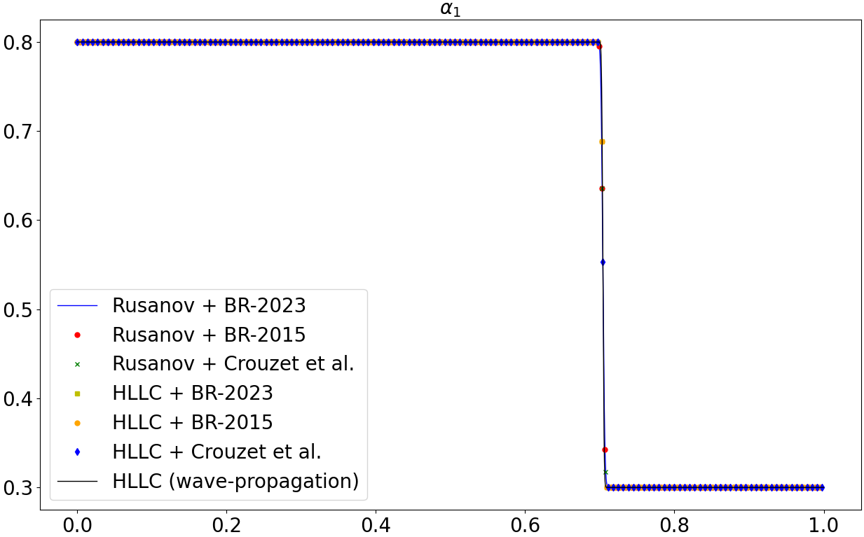
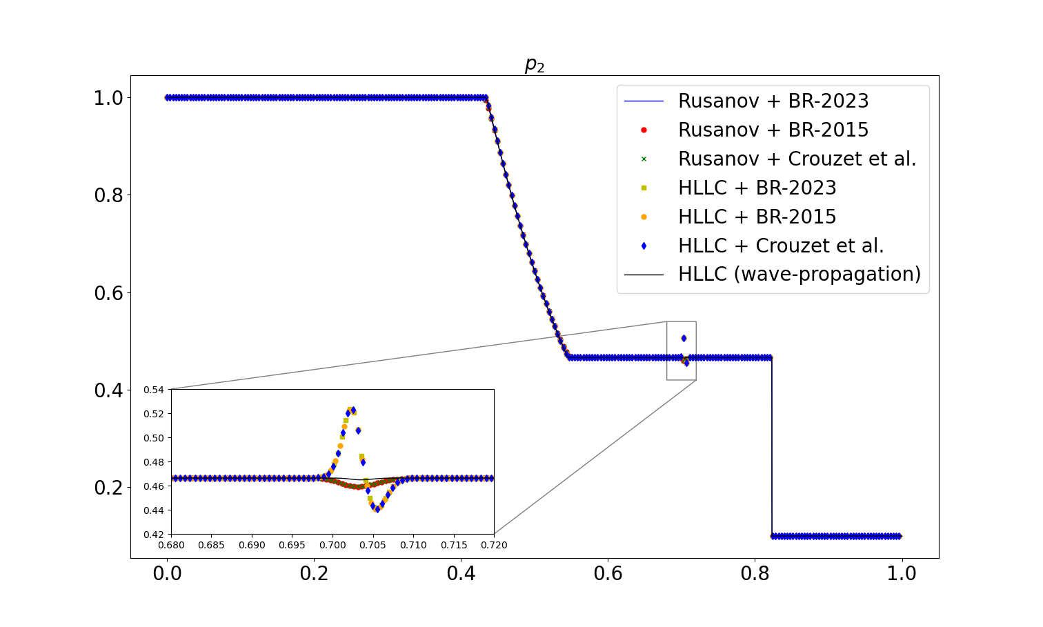
Figure 2: Sonic rarefaction test case with the fine mesh, results at $t=T_{f}$. Same description as Figure 1.

4.2 Low-density flow test case

Next, we consider another configuration inspired by a test case reported in [66]. More specifically, we employ test case 4, which is a two-phase extension of the so-called 123-problem [53, 67]. Both phases consist of two symmetric rarefaction waves and a stationary contact wave. The region between the rarefaction waves is close to vacuum. Hence, this is a severe test problem with a low-density flow. First, we employ the coarse mesh. The HLLC flux in combination with the approach proposed in [19] for the non-conservative terms of the energy equations does not preserve the thermodynamic admissibility of the flow variables and corrupted density values are generated. A positive solution is instead obtained employing the BR and the wave-propagation approach. We refer to the analysis proposed in Section 5 for a possible explanation of this result. Moreover, when coupled with a Rusanov flux, the BR approach yields a sharper description of the contact discontinuity with respect to the strategy presented in [19], in particular using the BR-2023 (32) (Figure 3).

Next, we employ the fine mesh. Analogous considerations to those reported in Section 4.1 are valid. However, one can notice that the Rusanov flux tends to smear the contact discontinuity out even at very high resolution (Figure 4).

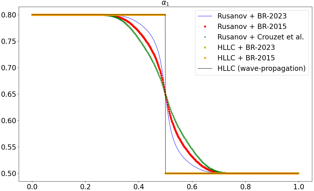
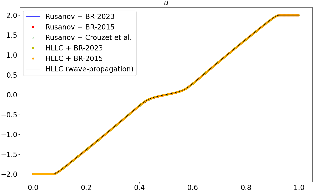
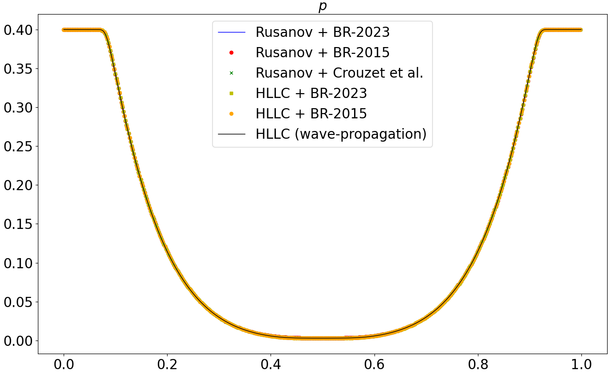
Figure 3: Low-density flow test case with the coarse mesh, results at $t=T_{f}$. Top-left: volume fraction of phase $1$. Top-right: velocity. Bottom-left: mixture density. Bottom-right: mixture pressure. Continuous black lines: HLLC-type wave-propagation scheme. Continuous blue lines: Rusanov flux in combination with BR approach (32). Red dots: Rusanov flux in combination with BR approach (33). Green crosses: Rusanov flux in combination with the approach proposed in [19]. Yellow squares: HLLC flux in combination with BR approach (32). Orange dots: HLLC flux in combination with the BR approach (33).

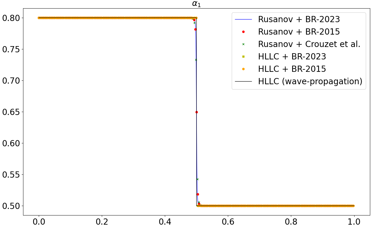
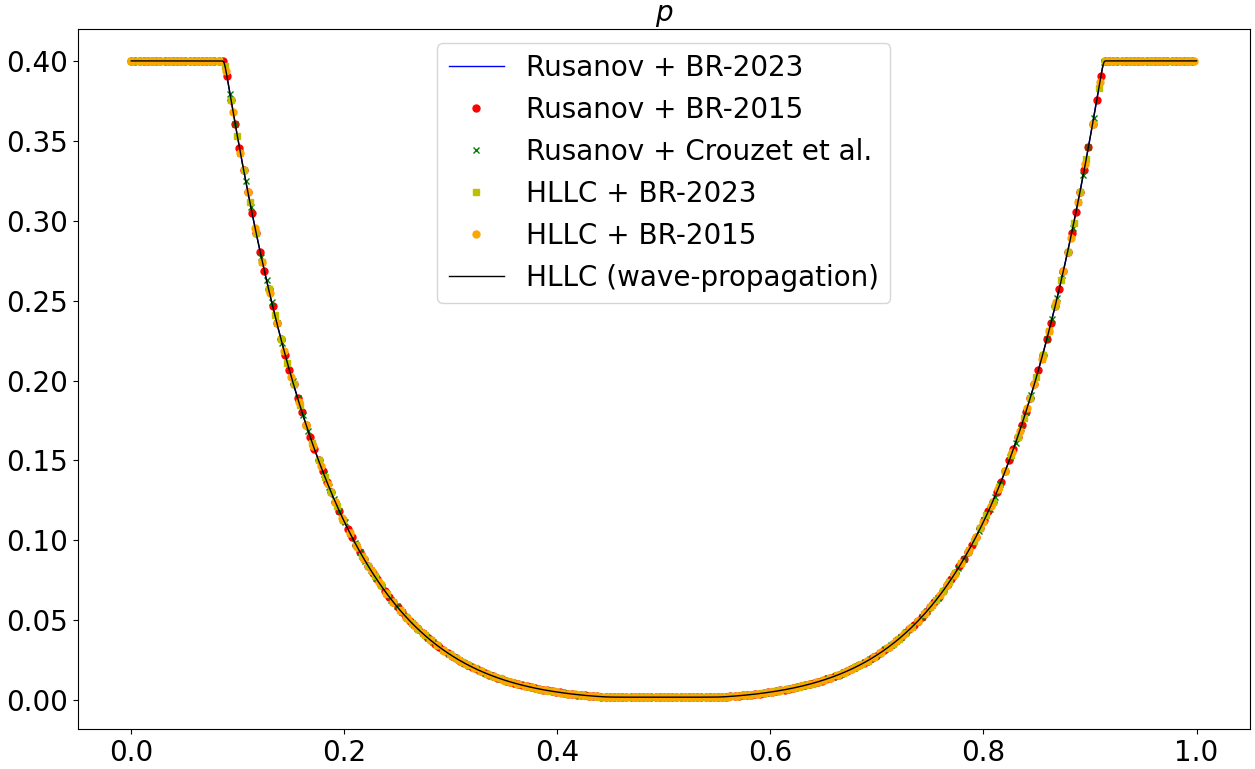
Figure 4: Low-density flow test case with the fine mesh, results at $t=T_{f}$. Same description as Figure 3.

4.3 Water-air shock tube

Next, we consider a water-air shock tube, analogous to those presented, e.g., in [52, 60, 62]. The shock tube is composed by two chambers each containing a nearly pure fluid (Tables 2-3). First, we employ the coarse mesh. For what concerns the Rusanov flux, a stable solution with positive volume fractions is established only for Courant numbers $C\leq 0.3$. Moreover, significant different results are obtained between the numerical methods, which are particularly evident from the velocity field (Figure 5).

Figure 5: Water-air shock tube test case with the coarse mesh, results at $t=T_{f}$. Top-left: volume fraction of phase $1$. Top-right: velocity. Bottom-left: Mixture density. Bottom-right: Mixture pressure. Continuous black lines: HLLC-type wave-propagation scheme. Blue diamonds: HLLC flux in combination with BR approach (32). Red dots: HLLC flux in combination with BR approach (33).

Next, we employ the fine mesh so as to achieve mesh convergence. Analogous considerations to those reported for the coarse mesh are valid (Figure 6). We also still notice visible differences in the results established with the BR-2023 (32) and the BR-2015 (33) for the treatment of the non-conservative terms. This behaviour is likely dependent on the absence of a well-defined set of Rankine-Hugoniot conditions for this model and therefore different numerical schemes can converge to different solutions.

Since this test case is characterized by quasi-pure phases, we compare our results, for the sake of completeness, with the analytical solution of the Riemann problem for the Euler equations. The analytical solution of the Riemann problem for the single-phase Euler equations governed by the SG-EOS (3) can be found, e.g., in [39]. One can easily notice that the numerical solution established with the HLLC-type wave-propagation scheme is closer to the analytical solution of the Euler equations compared to the other numerical schemes. This results may be related to the fact that the fluctuations (45) of the wave-propagation method are computed neglecting the non-conservative terms of the phasic total energies equations for the external 1-wave and 3-wave of the Riemann solution and the corresponding jump conditions reduce to the approximate jump relations of the 5-equation model presented in [52] (see the discussion in Section 3.1). The sensitivity of the shock location with respect to the numerical scheme of this model raises the question of the practical applicability — of the model or the considered numerical schemes — when no mechanical relaxation occurs, and by extension, when the mechanical relaxation occurs at finite rate only. We will show in Section 7 that the differences between the different numerical methods are significantly reduced when the instantaneous mechanical relaxation is considered, thus showing a limited sensitivity of the 5-equation model’s shock profiles to the numerical scheme for this configuration.

Figure 6: Water-air shock tube test case with the fine mesh, results at $t=T_{f}$. Same description as Figure 5.

Figure 7: Water-air shock tube test case with the fine mesh, results at $t=T_{f}$. Left: velocity. Right: zoom of the mixture density. Black lines: analytical solution of the Riemann problem for the Euler equations. Blue lines: HLLC-type wave-propagation method. Red lines: HLLC scheme in combination with BR approach (32).

4.4 Epoxy-spinel shock

In a final test, we consider the epoxy-spinel strong shock as presented in [52]. We employ the fine mesh, so as to achieve mesh convergence. A reasonable agreement is established between the different numerical methods (Figure 8). We point out that, in this test case, the non-conservative terms may play a more significant role compared to the previous test cases, since we are considering a mixture region instead of quasi-pure phases. However, one can easily notice visible differences in the phasic pressures in correspondence of the shock layer. We will further discuss this point in Section 7.3, where we show that these differences strongly influence the results obtained with the mechanical relaxation.

Figure 8: Epoxy-spinel shock test case with the fine mesh, results at $t=T_{f}$. Top-Left: pressure of phase $1$. Top-Right: zoom of the pressure of phase $1$. Bottom-Left: pressure of phase $2$. Bottom-Right: zoom of the pressure of phase $2$. Continuous black lines:: HLLC-type wave-propagation method. Continuous blue lines: Rusanov scheme in combination with BR approach (32). Red dots: HLLC scheme in combination with BR approach (32).

5 Reformulation of the BR approach in the framework of the path-conservative schemes

In this section, we analyze the BR approach and show that, among the possible variants considered, those which have proven to be the most robust in Section 4, can be recast into the framework of path-conservative schemes. The path-conservative method [48] has been originally developed for finite volume schemes [14, 48] and then extended to the Discontinuous Galerkin method [26, 27, 29, 32, 54]. We briefly recall some basic concepts. Consider again the non-conservative product $\mathbf{B}(w)\operatorname{\nabla}w$. Then, the path-conservative finite volume approximation on the element $K$ reads as follows

$$\int_{K}\mathbf{B}(w)\operatorname{\nabla}w\mathrm{d}\Omega\approx\int_{\partial K}\bm{\mathcal{D}}^{-}\left(w_{L},w_{R},\bm{n}\right)\mathrm{d}\Sigma,$$ (48)

where $\bm{n}$ denotes the outward unit normal vector from the element. Following [48], in order to obtain a $\Psi$-conservative scheme, the function $\bm{\mathcal{D}}$ is such that

$$\bm{\mathcal{D}}^{-}\left(w,w,\bm{n}\right)=0\quad\forall w,\bm{n},$$ (49a)

$$\bm{\mathcal{D}}^{-}\left(w_{L},w_{R},\bm{n}\right)+\bm{\mathcal{D}}^{+}\left(w_{L},w_{R},\bm{n}\right)=\left[\int_{0}^{1}\mathbf{B}\left(\Psi(w_{L},w_{R},s)\right)\frac{\partial{\Psi}}{\partial{s}}ds\right]\bm{n},$$ (49b)

where $\bm{\mathcal{D}}^{+}\left(w_{L},w_{R},\bm{n}\right)=\bm{\mathcal{D}}^{-}\left(w_{R},w_{L},-\bm{n}\right)$. The function $\Psi$ denotes a family of paths connecting $w_{L}$ and $w_{R}$ such that

$$\Psi(w_{L},w_{R},0) =w_{L},$$

$$\Psi(w_{L},w_{R},1) =w_{R},$$

$$\Psi(w,w,s) =w.$$

We refer to [48] for a detailed discussion of the regularity required by $\Psi$. For multidimensional systems, the path connecting the two states $w_{L}$ and $w_{R}$ may in principle depend also on $\bm{n}$, but if the system is invariant under rotations, this dependency can be dropped [16, 26]. Condition (49a) guarantees that if $\operatorname{\nabla}w=0$, then no contribution arises. Condition (49b) guarantees that if $\mathbf{B}$ represents the Jacobian of a flux, then a classical conservative scheme is retrieved [48]. We stress the fact that the wave-propagation scheme discussed in Section 3.4 fits into this formalism. Denote now

$$\bm{\mathcal{D}}^{-}\left(w_{L},w_{R},\bm{n}\right)=\left(\widehat{\mathbf{B}w}(w_{L},w_{R})-\widehat{\mathbf{B}}(w_{L},w_{R})w_{L}\right)\bm{n},$$ (50)

with $\widehat{\mathbf{B}w}(w_{L},w_{R})$ and $\widehat{\mathbf{B}}(w_{L},w_{R})$ as in (31). One can immediately notice that condition (49a) is fulfilled. Moreover,

$$\bm{\mathcal{D}}^{-}\left(w_{L},w_{R},\bm{n}\right)+\bm{\mathcal{D}}^{+}\left(w_{L},w_{R},\bm{n}\right)=\left[\widehat{\mathbf{B}}(w_{L},w_{R})\left(w_{R}-w_{L}\right)\right]\bm{n}.$$ (51)

If we consider a family of segments

$$\Psi=w_{L}+s\left(w_{R}-w_{L}\right),$$ (52)

condition (49b) reduces to

$$\bm{\mathcal{D}}^{-}\left(w_{L},w_{R},\bm{n}\right)+\bm{\mathcal{D}}^{+}\left(w_{L},w_{R},\bm{n}\right)=\left(w_{R}-w_{L}\right)\left[\int_{0}^{1}\mathbf{B}\left(\Psi(w_{L},w_{R},s)\right)\mathrm{d}s\right]\bm{n},$$ (53)

and therefore, considering $\widehat{\mathbf{B}}$ as an approximation of $\int_{0}^{1}\mathbf{B}\left(\Psi(w_{L},w_{R},s)\right)\mathrm{d}s$, we conclude that also condition (49b) is fulfilled. In particular, if we take

$$\widehat{\mathbf{B}}(w_{L},w_{R})=\frac{1}{2}\left(\mathbf{B}(w_{L})+\mathbf{B}(w_{R})\right),$$ (54)

this is equivalent to consider a trapezoidal rule for $\int_{0}^{1}\mathbf{B}\left(\Psi(w_{L},w_{R},s)\right)\mathrm{d}s$. The choice of a linear path is the standard one in the literature [2, 13, 29, 31, 32], even though more complex paths can be considered [22, 63], and also the choice of the trapezoidal rule to approximate the path integral is rather common [13, 31].

In conclusion, the BR approach can be seen as a particular approximate path-conservative scheme employing segments as paths. The BR approach has already been employed for the discretization of non-conservative terms in hyperbolic systems [46, 68] and the idea to consider a double integration by parts has been already adopted in several CFD applications to obtain well-balanced schemes in the so-called strong form [3, 5, 6, 69]. However, to the best of our knowledge, this is the first rigorous analysis that shows how a numerical strategy originally and typically employed for the discretization of diffusion operators [8, 47] is linked to a widely used framework for the discretization of hyperbolic non-conservative systems. Finally, one can immediately notice that the approach (38) proposed in [19] does not satisfy (49a) and therefore it cannot be reformulated in the framework of path-conservative schemes. This could explain why this approach is less robust for the solution of the homogeneous problem (11), as we have verified in Section 4.

6 Instantaneous mechanical relaxation

In this section, we discuss the relaxation of the phasic pressures obtained from the discretization of the hyperbolic operator towards an equilibrium value. Following the operator splitting approach depicted at the beginning of Section 3, we obtain the following system of ODEs

$$\frac{\mathrm{d}{\alpha_{1}}}{\mathrm{d}{t}} =\mu\left(p_{1}-p_{2}\right),$$ (55a)

$$\frac{\mathrm{d}{\alpha_{1}\rho_{1}}}{\mathrm{d}{t}} =0,$$ (55b)

$$\frac{\mathrm{d}{\alpha_{2}\rho_{2}}}{\mathrm{d}{t}} =0,$$ (55c)

$$\frac{\mathrm{d}{\rho\bm{u}}}{\mathrm{d}{t}} =0,$$ (55d)

$$\frac{\mathrm{d}{\alpha_{1}\rho_{1}E_{1}}}{\mathrm{d}{t}} =-\mu p_{I}\left(p_{1}-p_{2}\right),$$ (55e)

$$\frac{\mathrm{d}{\alpha_{2}\rho_{2}E_{2}}}{\mathrm{d}{t}} =\mu p_{I}\left(p_{1}-p_{2}\right).$$ (55f)

Combining (55a), (55e), and (55f), one obtains [51]

$$\frac{\mathrm{d}{\alpha_{1}\rho_{1}E_{1}}}{\mathrm{d}{t}} =-p_{I}\frac{\mathrm{d}{\alpha_{1}}}{\mathrm{d}{t}},$$ (56a)

$$\frac{\mathrm{d}{\alpha_{2}\rho_{2}E_{2}}}{\mathrm{d}{t}} =p_{I}\frac{\mathrm{d}{\alpha_{1}}}{\mathrm{d}{t}}.$$ (56b)

Here, we choose the following expression for the interfacial pressure

$$p_{I}=\frac{Z_{2}p_{1}+Z_{1}p_{2}}{Z_{1}+Z_{2}},$$ (57)

where $Z_{k}=\rho_{k}c_{k}$ corresponds to the phasic acoustic impedance.

In the following, for a given quantity $\chi$, we will denote by $\chi^{(0)}$ the value coming from the discretization of the hyperbolic operator, i.e. before the relaxation step, and by $\chi^{\star}$ the value at the mechanical equilibrium, i.e. after the relaxation process. In [51], the authors propose to consider a linear variation of the interfacial pressure $p_{I}$ as a function of the volume fraction $\alpha_{1}$, so that

$$p_{I}(\alpha_{1})=p_{I}^{(0)}+\frac{p_{I}^{\star}-p_{I}^{(0)}}{\alpha_{1}^{\star}-\alpha_{1}^{(0)}}\left(\alpha_{1}-\alpha_{1}^{(0)}\right),$$ (58)

Note that, as reported in [51], hypothesis (58) is equivalent to consider in (56a)-(56b)

$$p_{I}=\frac{1}{2}\left(p_{I}^{(0)}+p_{I}^{\star}\right).$$

Hence, using (58), equations (56a)-(56b) can be integrated so as to obtain

$$\alpha_{1}^{\star}\rho_{1}^{\star}E_{1}^{\star}-\alpha_{1}^{(0)}\rho_{1}^{(0)}E_{1}^{(0)} =-\frac{p_{I}^{(0)}+p_{I}^{\star}}{2}\left(\alpha_{1}^{\star}-\alpha_{1}^{(0)}\right),$$ (59a)

$$\alpha_{2}^{\star}\rho_{2}^{\star}E_{2}^{\star}-\alpha_{2}^{(0)}\rho_{2}^{(0)}E_{2}^{(0)} =\frac{p_{I}^{(0)}+p_{I}^{\star}}{2}\left(\alpha_{1}^{\star}-\alpha_{1}^{(0)}\right),$$ (59b)

or equivalently, since $\alpha_{k}^{\star}\rho_{k}^{\star}=\alpha_{k}^{(0)}\rho_{k}^{(0)}$ and $\bm{u}^{\star}=\bm{u}^{(0)}$,

$$e_{1}^{\star}-e_{1}^{(0)} =-\frac{p_{I}^{(0)}+p_{I}^{\star}}{2}\frac{\alpha_{1}^{\star}-\alpha_{1}^{(0)}}{\alpha_{1}^{(0)}\rho_{1}^{(0)}},$$ (60a)

$$e_{2}^{\star}-e_{2}^{(0)} =\frac{p_{I}^{(0)}+p_{I}^{\star}}{2}\frac{\alpha_{1}^{\star}-\alpha_{1}^{(0)}}{\alpha_{2}^{(0)}\rho_{2}^{(0)}}.$$ (60b)

Next, imposing instantaneous mechanical equilibrium, i.e. $p_{1}^{\star}=p_{2}^{\star}=p^{\star}$, (59a)-(59b) reduce to a system of two equations in the two unknowns $p^{\star}$ and $\alpha_{1}^{\star}$. The mixture specific internal energy $e$ is defined as

$$\rho e=\alpha_{1}\rho_{1}e_{1}+\alpha_{2}\rho_{2}e_{2}.$$ (61)

The latter relation, assuming $p_{1}=p_{2}=p$ in the phasic pressure laws, determines implicitly the mixture pressure law

$$p=p\left(e,\rho_{1},\rho_{2},\alpha_{1}\right).$$

In the case of the SG-EOS, we obtain an explicit expression for the mixture pressure [4, 51, 60]

$$p=p\left(e,\rho_{1},\rho_{2},\alpha_{1}\right)=\frac{\rho e-\left(\alpha_{1}\rho_{1}\eta_{1}+\alpha_{2}\rho_{2}\eta_{2}\right)-\left(\frac{\alpha_{1}\gamma_{1}\pi_{1}}{\gamma_{1}-1}+\frac{\alpha_{2}\gamma_{2}\pi_{2}}{\gamma_{2}-1}\right)}{\frac{\alpha_{1}}{\gamma_{1}-1}+\frac{\alpha_{2}}{\gamma_{2}-1}}.$$ (62)

It is worth to remark that, thanks to the use of phasic total energies for the homogeneous system (11), the numerical method guarantees that the relaxed pressure $p^{\star}$ verifies the mixture pressure law and satisfies by construction the conservation of the mixture energy, i.e. it is mixture-energy consistent [51]. In the specific case of the SG-EOS, a quadratic equation of the form

$$a\left(p^{\star}\right)^{2}+bp^{\star}+c=0,$$

is obtained for the relaxed pressure $p^{\star}$, with

$$a= 1+\gamma_{2}\alpha_{1}^{(0)}+\gamma_{1}\alpha_{2}^{(0)},$$

$$b= \left(2\gamma_{1}\pi_{1}+\left(\gamma_{1}-1\right)p_{I}^{(0)}\right)\alpha_{2}^{(0)}+\left(2\gamma_{2}\pi_{2}+\left(\gamma_{2}-1\right)p_{I}^{(0)}\right)\alpha_{1}^{(0)}$$

$$-\left(1+\gamma_{2}\right)\alpha_{1}^{(0)}p_{1}^{(0)}-\left(1+\gamma_{1}\right)\alpha_{2}^{(0)}p_{2}^{(0)},$$ (63)

$$c= -\left(2\gamma_{2}\pi_{2}+\left(\gamma_{2}-1\right)p_{I}^{(0)}\right)\alpha_{1}^{(0)}p_{1}^{(0)}-\left(2\gamma_{1}\pi_{1}+\left(\gamma_{1}-1\right)p_{I}^{(0)}\right)\alpha_{2}^{(0)}p_{2}^{(0)}.$$

Moreover, the value of the volume fraction at the equilibrium $\alpha_{1}^{\star}$ is [51]

$$\alpha_{1}^{\star}=\alpha_{1}^{(0)}\frac{\left(\gamma_{1}-1\right)p^{\star}+2p_{1}^{(0)}+2\gamma_{1}\pi_{1}+\left(\gamma_{1}-1\right)p_{I}^{(0)}}{\left(\gamma_{1}+1\right)p^{\star}+2\gamma_{1}\pi_{1}+\left(\gamma_{1}-1\right)p_{I}^{(0)}}.$$ (64)

As evident from this short presentation, the relaxation process depends on the choice of interfacial pressure $p_{I}$. Moreover, once a choice of the interfacial pressure is made, several approximation techniques for the relaxation process are available. Both the choice of the interfacial pressure and the numerical discretization of the relaxation operator may affect the post-relaxation state and impact the global robustness and accuracy of the numerical scheme. We refer to [33] for a detailed discussion of the impact of different choices for the interfacial pressure and its numerical analysis. In the present work, we consider a single choice interfacial pressure given by (57) and the corresponding numerical relaxation procedure described above. We remark that in the current method, without any form of implicitation, i.e. if $p_{I}^{\star}$ is not employed in the definition of $p_{I}$ for (59a)-(59b), the positivity of the thermodynamic state may be lost for the proposed relaxation methods [33].

7 Numerical results with mechanical relaxation

In this section, we analyze the approaches for the instantaneous mechanical relaxation depicted in Section 6 and their interaction with the numerical strategies for the hyperbolic operator.

7.1 Water-air shock tube

As a first test case of this section, we consider the instantaneous mechanical relaxation for the water-air shock tube described in Section 4.3. We employ the fine mesh. The solution obtained considering the approximated jump relations for the 5-equation model of Kapila is reported for reference. A good agreement is established for all the schemes, in particular for what concerns the HLLC-type schemes (Figure 9). Notice that, when the mechanical relaxation is considered, we can establish a stable solution with the Rusanov flux also at $C=0.9$. One can easily notice that the HLLC-type wave-propagation scheme and the HLLC for the conservative portion of the system in combination with the treatment of the non-conservative terms converge towards the same numerical solution.

Figure 9: Water-air shock tube test case with instantaneous mechanical relaxation, results at $t=T_{f}$. Top-left: mixture density. Top-right: zoom of the mixture density. Bottom-left: velocity. Bottom-right: zoom of the velocity. Continuous black lines: solution obtained using the approximated jump conditions in [52]. Continuous blue lines: HLLC-type wave-propagation scheme. Continuous magenta lines: Rusanov flux in combination with BR approach (32). Green dots: Rusanov flux in combination with BR approach (33). Red squares: HLLC flux in combination with BR approach (32). Orange dots: HLLC flux in combination with BR approach (33).

7.2 Water cavitation tube

Next, we consider a water liquid-vapour cavitation (expansion) tube problem as presented in [51]. The liquid, which we conventionally denote with phase $1$, contains a uniformly distributed small amount of vapour, i.e. phase $2$ (Table 3). We focus on the instantaneous mechanical relaxation and we employ the fine mesh. The solution consists of two rarefactions propagating in opposite directions and producing a pressure decrease in the middle of the tube [51]. An analytical solution is available for this test case. A good agreement is established between the different numerical strategies and with the analytical solution (Figure 10). However, we notice visible differences in correspondence of the contact discontinuity (Figure 10), in particular for what concerns the volume fraction and the mixture density. This result further confirms the robustness of the approaches employed in this work. Indeed, this test case is characterized by low values of the vapour volume fraction $\alpha_{2}$ and can be subject to the formation of the vacuum state [67].

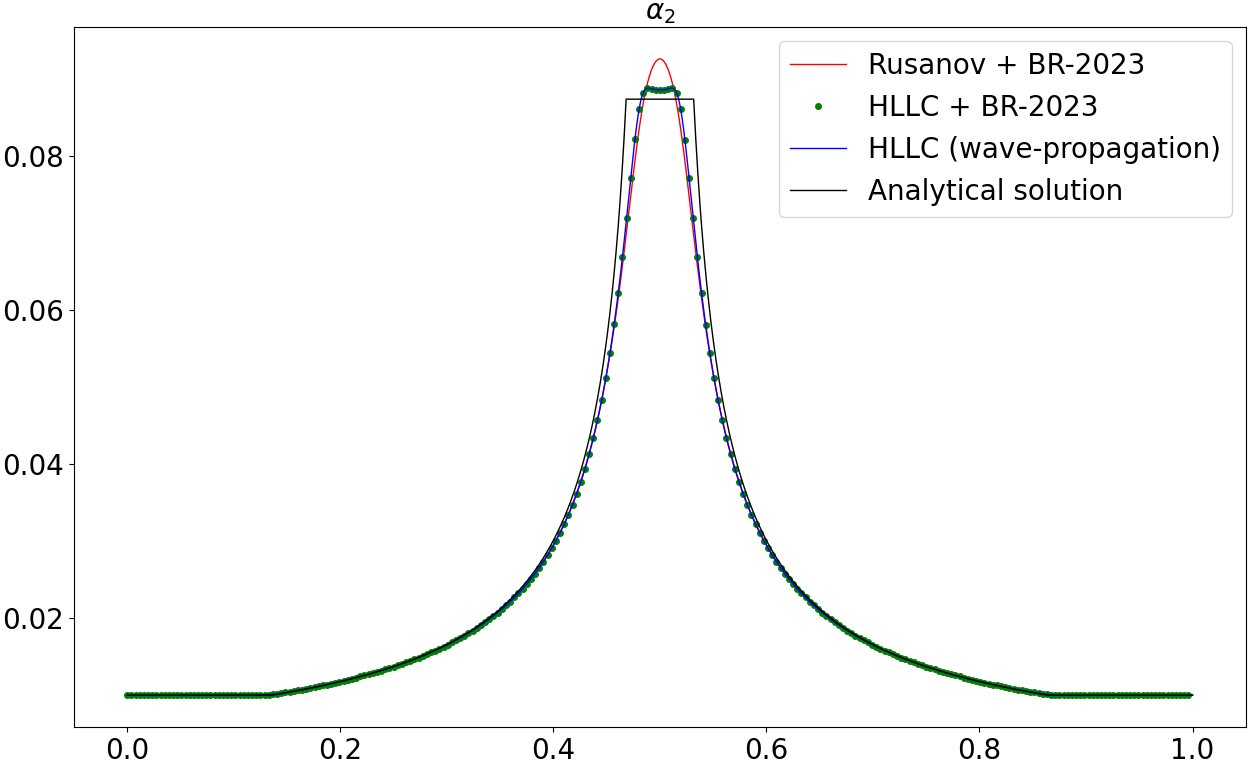
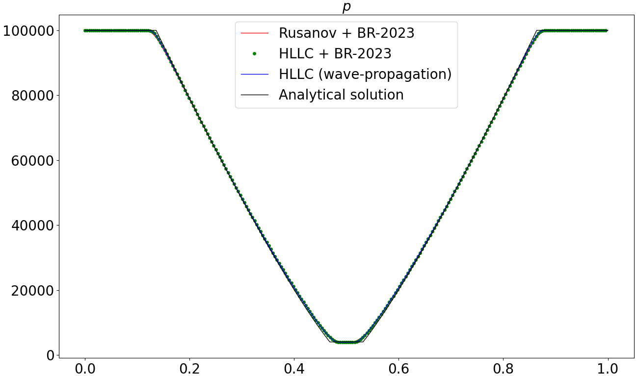
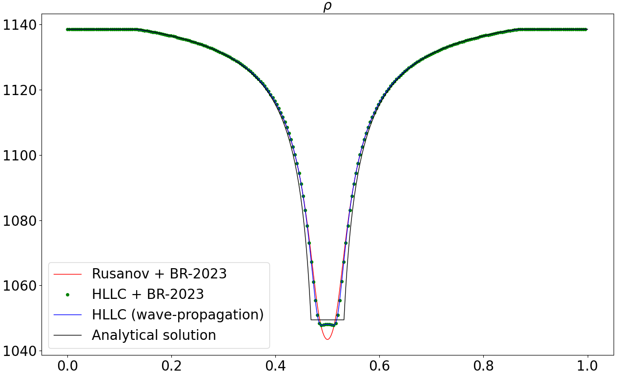
a)

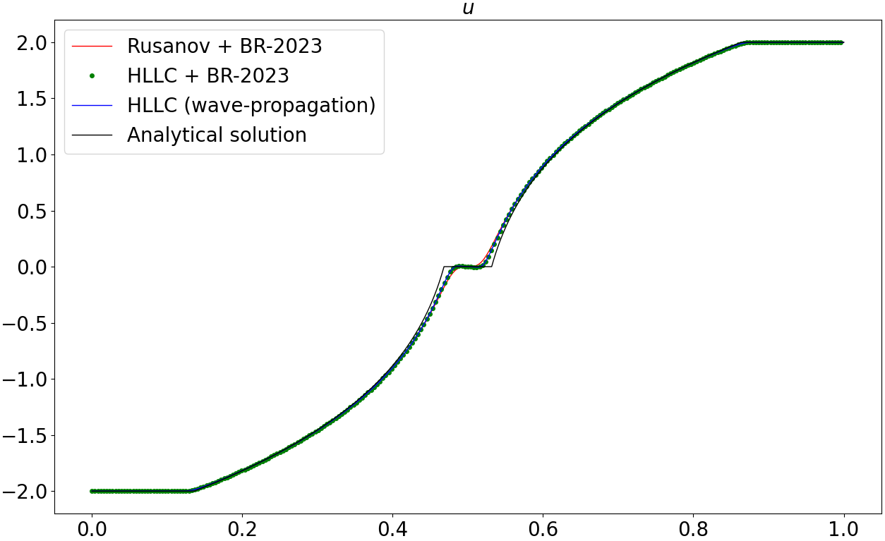
Figure 10: Double rarefaction test case with the fine mesh, results at $t=T_{f}$. Top-left: volume fraction of phase $2$. Top-right: mechanical equilibrium pressure. Bottom-left: mixture density. Bottom-right: velocity. Continuous black lines: analytical results. Continuous blue lines: HLLC-type wave-propagation scheme. Continuous red lines: Rusanov flux in combination with BR approach (32). Green dots: HLLC flux in combination with BR approach (32).

7.3 Epoxy-spinel shock

Next, we consider the epoxy-spinel strong shock already introduced in Section 4.4. We employ the fine mesh, so as to achieve mesh convergence. One can easily verify that the solution does not converge to the solution obtained using the approximated jump conditions in [52] (Figure 11). As discussed in [52], the approximated jump relations are valid only in the case of a weak shock. This discrepancy depends on the partition of internal energy in the shock layer (see the discussions in [52, 60]). The convergence value of the intermediate state of the volume fraction for the Riemann problem is strongly affected by the choice of the numerical flux for the conservative part and visible differences arise also between the HLLC-type wave-propagation scheme and the combination with the BR approach (Figure 11). Note that this result is totally dependent on the interaction between the numerical method employed to solve the homogeneous problem (11) and the mechanical relaxation. A uniform volume fraction is indeed imposed as initial condition (see Table 2) and therefore, without relaxation, the initial value is preserved. Moreover, we recall that in this test case we are dealing with a mixture region rather than quasi-pure phases and therefore non-conservative terms may have a greater impact.

In order to further analyze this behaviour, we consider different initial pressure ratios, i.e. we set for the initial conditions

$$p_{1,L}=p_{2,L}=\left\{10^{6},10^{7},10^{8},10^{9},10^{10},5\times 10^{10},10^{11}\right\}.$$

One can notice that visible difference arise starting from $p_{1,L}/p_{1,R}=p_{2,L}/p_{2,R}=5\times 10^{5}$ (Figure 12). The value predicted by the approximated jump relations in [52] is added for reference. This result reflects the absence of a complete set of well-defined Rankine-Hugoniot conditions for the 5-equation model proposed in [38]. The main result for this test case is that the differences observed in the volume fraction field are quite moderate when compared to the extreme pressure ratio needed to generate them. It thus shows that the theoretical shortcomings of the model, i.e. non-uniqueness of shock profiles, has only a limited impact in practical applications. The use of robust numerical strategies allows to obtain physically relevant numerical solutions.

Figure 11: Epoxy-spinel shock test case with the fine mesh, results at $t=T_{f}$. Top-left: volume fraction of phase $1$. Top-right: mechanical equilibrium pressure. Bottom-left: mixture density. Bottom-right: velocity. Continuous black lines: solutions obtained using the approximated jump relations in [52]. Continuous blue lines: HLLC-type wave-propagation scheme. Continuous red lines: Rusanov flux in combination with BR approach (32). Green dots: HLLC flux in combination with BR approach (32).

Figure 12: Epoxy-spinel shock test case with the fine mesh, intermediate state of the volume fraction ($y$-coordinate) as a function of the initial pressure ratio ($x$-coordinate), results at $t=T_{f}$. The continuous black line shows the value predicted by the approximated jump relations in [52]. The black dots report the results obtained using the HLLC-type wave-propagation scheme, the blue crosses show the results obtained using the HLLC flux in combination with the BR approach (32) for the non-conservative terms of the energy equations, whereas the red square represent the results obtained using the Rusanov flux in combination with the BR approach (32) for non-conservative terms.

7.4 2D Riemann problem

In a final test, we consider a two-dimensional Riemann problem inspired from the configuration C1 employed for the full BN model in [24] and analyzed also in [23, 28]. The computational domain is $\Omega=\left(-0.5,0.5\right)\times\left(0.5,0.5\right)$. The EOS parameters are $\gamma_{1}=\gamma_{2}=1.4,\pi_{1}=\pi_{2}=0,\eta_{1}=\eta_{2}=0$. The initial conditions are reported in Table 4. The final time is $T_{f}=$0.15\text{\,}\mathrm{s}$$. Following [24], we adopt reflective boundary conditions. In order to enhance the computational efficiency, the multiresolution capabilities of samurai [9] are employed. More specifically, we consider a minimum resolution which would correspond to a uniform mesh with $N_{\text{cells}}=256$ per direction and maximum resolution which would correspond to a uniform mesh with $N_{\text{cells}}=2048$ per direction, i.e. $2048^{2}\approx 4\cdot 10^{6}$ cells. The Courant number is set to $C=0.45$.

	$\alpha_{1}$	$\rho_{1}$	$p_{1}$	$u$	$v$	$\rho_{2}$	$p_{2}$
$\mathbf{Q}_{1}:\left(x>0,y>0\right)$	$0.8$	$2.0$	$2.0$	$0.0$	$0.0$	$1.5$	$2.0$
$\mathbf{Q}_{2}:\left(x<0,y>0\right)$	$0.4$	$1.0$	$1.0$	$0.0$	$0.0$	$0.5$	$1.0$
$\mathbf{Q}_{3}:\left(x<0,y<0\right)$	$0.8$	$2.0$	$2.0$	$0.0$	$0.0$	$1.5$	$2.0$
$\mathbf{Q}_{4}:\left(x>0,y<0\right)$	$0.4$	$1.0$	$1.0$	$0.0$	$0.0$	$0.5$	$1.0$

Table 4: Initial conditions for the 2D Riemann problem.

A good agreement is established between all the numerical methods (Figure 13) and with the results presented in [24]. This confirms the robustness of the computational framework presented in this work. Finally, we point out that the final computational meshes of the HLLC-based schemes are characterized by a slightly higher number of cells than that obtained using the Rusanov scheme (Figure 14). To avoid any misconception about this result, we recall that the basic principle of the multiresolution is that of data compression [9, 35]. The flow fields are decomposed on a local wavelet basis, which allows to quantify their local regularity and identify regions in which the data can be compressed without loss of information — up to a pre-defined tolerance. Hence, since the Rusanov scheme is more diffusive, it captures less flow features, thus allowing for a higher-compression rate of the mesh. In particular, the more smeared interface that we observe with the Rusanov scheme (bottom left plot of Figure 13) is a consequence of its higher numerical diffusion and not the coarser mesh.

Figure 13: 2D Riemann problem test case, results at $t=T_{f}$. Left column: volume fraction of phase $1$. Right column: mixture density. Top: HLLC-type wave-propagation. Middle: HLLC flux in combination with BR approach (32). Bottom: Rusanov in combination with BR approach (32).

Figure 14: 2D Riemann problem test case, computational mesh at different refinement levels at $t=T_{f}$. Top-left: HLLC-type wave-propagation scheme ($N_{\text{cells}}=134518$). Top-right: HLLC flux in combination with BR approach (32) ($N_{\text{cells}}=135536$). Bottom: Rusanov flux in combination with BR approach (32) ($N_{\text{cells}}=131590$). Level 8 corresponds to the minimum resolution, equivalent to a uniform mesh with $N_{\text{cells}}=256$ per direction, whereas level 11 corresponds to the maximum resolution, equivalent to a uniform mesh with $N_{\text{cells}}=2048$ per direction.

8 Conclusions

We have presented a robust computational framework for the 5-equation model of Kapila [38] by means of the mixture-energy-consistent 6-equation two-phase flow model with instantaneous mechanical relaxation terms. We have shown that, despite the absence of uniquely defined shock profiles for the considered models, correct numerical solutions can be obtained for practical cases through the use of robust and accurate numerical methods. To achieve this result, we have compared different numerical methods for the discretization of the homogeneous system (11), which rely on different treatments of the non-conservative terms. One of these treatments is based on a Bassi-Rebay (BR) approach [8]. We have shown here for the first time that this strategy, typically employed for diffusion-type operators, can be reformulated in the framework of the path-conservative schemes, which are widely employed for the discretization of non-conservative hyperbolic systems.

First, we have compared the results obtained for the homogeneous model, using the HLLC approximate Riemann solvers with the wave-propagation method, and the Rusanov and HLLC approximate Riemann solvers in combination with BR approach or the approximation proposed in [19] for the discretization of non-conservative terms. Since the model does not admit a complete set of Rankine-Hugoniot conditions uniquely defined, the construction of Riemann solvers is not straightforward. We have presented in this work some insights on the construction of approximate Riemann solvers so as to clarify the adopted underlying hypotheses. The approach proposed in [19] does not guarantee in general a positive solution and indeed is not consistent with the path-conservative scheme. Once mesh convergence is achieved, the remaining strategies do not converge in general to the same numerical solution for the homogeneous model. Moreover, even though kinetic equilibrium is prescribed, the results in general slightly differ from those obtained if one employs the full Baer-Nunziato (BN) model, as done in [66]. Finally, we have shown in the test case of a water-air shock tube that different numerical methods converge towards different solutions. This result raises the question of the use of the 6-equation model without mechanical relaxation or when finite-rate relaxation occurs, as, e.g., in [62]. Moreover, for this test case, Rusanov-based schemes need a lower Courant number to achieve a stable solution, whereas standard restrictions occur for the HLLC-based schemes. Hence, HLLC-based schemes are in general more robust for the numerical solution of the 6-equation model.

Next, we have focused on the case where instantaneous mechanical relaxation towards equilibrium is accounted for. In this case, for most configurations, all the methods tend in general towards the same approximate solution. However, when extreme pressure ratios are considered, different numerical schemes may tend towards different numerical solutions. A similar dependence of the numerical solution to the numerical parameters has also been observed in [33] for this case, as different interfacial pressures lead to different shock profiles at extreme pressure ratios in the epoxy-spinel test case. This result depends on the absence of a well-defined set of Rankine-Hugoniot conditions. Nevertheless, the observed differences are moderate in comparison with the pressure ratios required to generate them, and therefore, for most applications, this shortcoming of the model might not have a huge impact, even though it should be taken into account.

In this work, we have achieved mesh convergence with first order schemes, so as to avoid any further dependence of higher order methods related to reconstruction, limiters, and large stencils. The primary goal of this work is indeed to perform a detailed comparison between different discretization strategies for the mixture-energy-consistent 6-equation two-phase model in terms of accuracy and robustness and to analyze their non-trivial interaction with the instantaneous mechanical relaxation. The numerical results have been obtained using a number of cells that is unfeasible for practical applications with the ultimate goal to highlight the possible limitations of the model when mesh convergence is really established. In future work, we aim at analyzing the high-order extension of some of the presented discretization methods. The outcomes of this work also show that, although good results can be obtained when instantaneous mechanical relaxation is applied, without instantaneous mechanical relaxation, an unphysical dependence to the discretization method is observed. As such, for cases in which pressure non-equilibrium effects are relevant, the 6-equation model may not have the sufficient mathematical properties for practical use. For this reason, we aim at developing a numerical strategy for fully out-of-equilibrium flows, starting from the 7-equation model of Baer-Nunziato [7], or a recently derived all-topology two-fluid model [34], with source terms. These models are well posed, in the sense that non-conservative products are uniquely defined and they admit a mixture entropy inequality to select physically relevant weak solutions [30, 34]. This approach can lead to a more rigorous mathematical treatment, even though certainly increasing the computational burden. Finally, in the framework of the BN model, coupled finite-rate kinetic, mechanical, and thermal relaxation techniques have been recently developed in [36], however, the correct scaling of the different characteristic time-scales involved is still an open problem.

References

- [1] R. Abgrall, P. Bacigaluppi and S. Tokareva “A high-order nonconservative approach for hyperbolic equations in fluid dynamics” In Computers & Fluids 169 Elsevier, 2018, pp. 10–22
- [2] R. Abgrall and S. Karni “A comment on the computation of non-conservative products” In Journal of Computational Physics 229 Elsevier, 2010, pp. 2759–2763
- [3] R. Abgrall and M. Ricchiuto “High order methods for CFD” In Encyclopedia of Computational Mechanics John Wiley & Sons, Ltd, 2017
- [4] G. Allaire, S. Clerc and S. Kokh “A five-equation model for the simulation of interfaces between compressible fluids” In Journal of Computational Physics 181 Elsevier, 2002, pp. 577–616
- [5] L. Arpaia, M. Ricchiuto, A.G. Filippini and R. Pedreros “An efficient covariant frame for the spherical shallow water equations: well balanced DG approximation and application to tsunami and storm surge” In Ocean Modelling 169 Elsevier, 2022, pp. 101915
- [6] L. Arpaia, G. Orlando, C. Ferrarin and L. Bonaventura “A high-order matrix-free adaptive solver for the shallow water equations with irregular bathymetry”, 2025 arXiv: https://arxiv.org/abs/2505.18743
- [7] M.R. Baer and J.W. Nunziato “A two-phase mixture theory for the deflagration-to-detonation transition (DDT) in reactive granular materials” In International Journal of Multiphase Flow 12, 1986, pp. 861–889
- [8] F. Bassi and S. Rebay “A High-order accurate discontinuous finite element method for the numerical solution of the compressible Navier-Stokes equations” In Journal of Computational Physics 131, 1997, pp. 267–279
- [9] T. Bellotti, L. Gouarin, B. Graille and M. Massot “Multidimensional fully adaptive lattice Boltzmann methods with error control based on multiresolution analysis” In Journal of Computational Physics 471 Elsevier, 2022, pp. 111670
- [10] S. Bianchini and A. Bressan “Vanishing viscosity solutions of nonlinear hyperbolic systems” In Annals of mathematics 161, 2005, pp. 223–342
- [11] F. Bouchut “Nonlinear stability of finite Volume Methods for hyperbolic conservation laws: And Well-Balanced schemes for sources” Springer Science & Business Media, 2004
- [12] F. Bouchut and T.M. Luna “An entropy satisfying scheme for two-layer shallow water equations with uncoupled treatment” In ESAIM: Mathematical Modelling and Numerical Analysis 42 EDP Sciences, 2008, pp. 683–698
- [13] S. Busto, M. Dumbser, S. Gavrilyuk and K. Ivanova “On thermodynamically compatible finite volume methods and path-conservative ADER discontinuous Galerkin schemes for turbulent shallow water flows” In Journal of Scientific Computing 88.1 Springer, 2021, pp. 28
- [14] M. Castro, J. Gallardo and C. Parés “High order finite volume schemes based on reconstruction of states for solving hyperbolic systems with nonconservative products. Applications to shallow-water systems” In Mathematics of computation 75.255, 2006, pp. 1103–1134
- [15] M.J. Castro, P.G. LeFloch, M.L. Muñoz-Ruiz and C. Parés “Why many theories of shock waves are necessary: Convergence error in formally path-consistent schemes” In Journal of Computational Physics 227.17 Elsevier, 2008, pp. 8107–8129
- [16] M.J. Castro et al. “High order extensions of Roe schemes for two-dimensional nonconservative hyperbolic systems” In Journal of Scientific Computing 39 Springer, 2009, pp. 67–114
- [17] C. Chalons and F. Coquel “A new comment on the computation of non-conservative products using Roe-type path conservative schemes” In Journal of Computational Physics 335 Elsevier, 2017, pp. 592–604
- [18] F. Coquel, J.-M. Hérard and K. Saleh “A positive and entropy-satisfying finite volume scheme for the Baer-Nunziato model” In Journal of Computational Physics 330 Elsevier, 2017, pp. 401–435
- [19] F. Crouzet et al. “Approximate solutions of the Baer-Nunziato model” In ESAIM: Proceedings 40, 2013, pp. 63–82 EDP Sciences
- [20] G. Dal Maso, P.G. LeFloch and F. Murat “Definition and weak stability of nonconservative products” In Journal de Mathématiques Pures et Appliquées 74, 1995, pp. 483–548
- [21] S.F. Davis “Simplified Second-Order Godunov-Type Methods” In SIAM Journal on Scientific and Statistical Computing 9, 1988, pp. 445–473
- [22] M. De Lorenzo, M. Pelanti and Ph. Lafon “HLLC-type and path-conservative schemes for a single-velocity six-equation two-phase flow model: A comparative study” In Applied Mathematics and Computation 333 Elsevier, 2018, pp. 95–117
- [23] M. Dumbser and D.S. Balsara “A new efficient formulation of the HLLEM Riemann solver for general conservative and non-conservative hyperbolic systems” In Journal of Computational Physics 304 Elsevier, 2016, pp. 275–319
- [24] M. Dumbser and W. Boscheri “High-order unstructured Lagrangian one-step WENO finite volume schemes for non-conservative hyperbolic systems: applications to compressible multi-phase flows” In Computers & Fluids 86 Elsevier, 2013, pp. 405–432
- [25] M. Dumbser and E.F. Toro “A simple extension of the Osher Riemann solver to non-conservative hyperbolic systems” In Journal of Scientific Computing 48 Springer, 2011, pp. 70–88
- [26] M. Dumbser, M. Castro, C. Parés and E.F. Toro “ADER schemes on unstructured meshes for nonconservative hyperbolic systems: Applications to geophysical flows” In Computers & Fluids 38.9 Elsevier, 2009, pp. 1731–1748
- [27] M. Dumbser et al. “FORCE schemes on unstructured meshes II: Non-conservative hyperbolic systems” In Computer Methods in Applied Mechanics and Engineering 199.9-12 Elsevier, 2010, pp. 625–647
- [28] F. Fraysse, C. Redondo, G. Rubio and E. Valero “Upwind methods for the Baer-Nunziato equations and higher-order reconstruction using artificial viscosity” In Journal of Computational Physics 326 Elsevier, 2016, pp. 805–827
- [29] E. Gaburro, W. Boscheri, S. Chiocchetti and M. Ricchiuto “Discontinuous Galerkin schemes for hyperbolic systems in non-conservative variables: quasi-conservative formulation with subcell finite volume corrections” In Computer Methods in Applied Mechanics and Engineering 431 Elsevier, 2024, pp. 117311
- [30] T. Gallouët, J.-M. Hérard and N. Seguin “Numerical modeling of two-phase flows using the two-fluid two-pressure approach” In Mathematical Models and Methods in Applied Sciences 14.05 World Scientific, 2004, pp. 663–700
- [31] F. Gatti et al. “A scalable well-balanced numerical scheme for the modeling of two-phase shallow granular landslide consolidation” In Journal of Computational Physics 501 Elsevier, 2024, pp. 112798
- [32] E. Guerrero Fernández, M.J. Castro Díaz, Mi. Dumbser and T. Luna “An arbitrary high order well-balanced ADER-DG numerical scheme for the multilayer shallow-water model with variable density” In Journal of Scientific Computing 90.1 Springer, 2022, pp. 52
- [33] W. Haegeman, J. Dupays, C. Le Touze and M. Massot “Numerical methods and relaxation techniques for diffuse interface models in high-velocity two-phase flow simulations”, 2024 DOI: 10.23967/eccomas.2024.071
- [34] W. Haegeman, G. Orlando, S. Kokh and M. Massot “An all-topology two-fluid model for two-phase flows derived through Hamilton’s Stationary Action Principle”, 2025 URL: https://hal.science/hal-05249139
- [35] A. Harten “Multiresolution Algorithms for the Numerical Solution of Hyperbolic Conservation Laws” In Communications on Pure and Applied Mathematics 48.12, 1995, pp. 1305–1342
- [36] J.-M. Hérard and G. Jomée “Two approaches to compute unsteady compressible two-phase flow models with stiff relaxation terms” In ESAIM: Mathematical Modelling and Numerical Analysis 57.6 EDP Sciences, 2023, pp. 3537–3583
- [37] T.Y. Hou and P.G. LeFloch “Why nonconservative schemes converge to wrong solutions: error analysis” In Mathematics of computation 62, 1994, pp. 497–530
- [38] A.K. Kapila et al. “Two-phase modeling of deflagration-to-detonation transition in granular materials: Reduced equations” In Physics of fluids 13 American Institute of Physics, 2001, pp. 3002–3024
- [39] D.I. Ketcheson, R.J. LeVeque and M.J. Del Razo “Riemann problems and Jupyter solutions” SIAM, 2020
- [40] D.I. Ketcheson, M. Parsani and R.J. LeVeque “High-order wave propagation algorithms for hyperbolic systems” In SIAM Journal on Scientific Computing 35 SIAM, 2013, pp. A351–A377
- [41] O. Le Métayer and R. Saurel “The Noble-Abel Stiffened-Gas equation of state” In Physics of Fluids 28, 2016, pp. 046102
- [42] R.J. LeVeque “Finite volume methods for hyperbolic problems” Cambridge University Press, 2002
- [43] H. Lochon, F. Daude, P. Galon and J.-M. Hérard “HLLC-type Riemann solver with approximated two-phase contact for the computation of the Baer-Nunziato two-fluid model” In Journal of Computational Physics 326 Elsevier, 2016, pp. 733–762
- [44] A. Murrone and H. Guillard “A five equation reduced model for compressible two phase flow problems” In Journal of Computational Physics 202 Elsevier, 2005, pp. 664–698
- [45] N.T. Nguyen and M. Dumbser “A path-conservative finite volume scheme for compressible multi-phase flows with surface tension” In Applied Mathematics and Computation 271 Elsevier, 2015, pp. 959–978
- [46] G. Orlando “Modelling and simulations of two-phase flows including geometric variables” http://hdl.handle.net/10589/198599, 2023
- [47] S. Ortleb “A comparative Fourier analysis of discontinuous Galerkin schemes for advection-diffusion with respect to BR1, BR2, and local discontinuous Galerkin diffusion discretization” In Mathematical Methods in the Applied Sciences 43.13 Wiley Online Library, 2020, pp. 7841–7863
- [48] C. Parés “Numerical methods for nonconservative hyperbolic systems: a theoretical framework” In SIAM Journal on Numerical Analysis 44 SIAM, 2006, pp. 300–321
- [49] M. Pelanti “Wave structure similarity of the HLLC and Roe Riemann solvers: Application to low Mach number preconditioning” In SIAM Journal on Scientific Computing 40.3 SIAM, 2018, pp. A1836–A1859
- [50] M. Pelanti “Arbitrary-rate relaxation techniques for the numerical modeling of compressible two-phase flows with heat and mass transfer” In International Journal of Multiphase Flow 153, 2022, pp. 104097
- [51] M. Pelanti and K.-M. Shyue “A mixture-energy-consistent six-equation two-phase numerical model for fluids with interfaces, cavitation and evaporation waves” In Journal of Computational Physics 259 Elsevier, 2014, pp. 331–357
- [52] F. Petitpas, E. Franquet, R. Saurel and O. Le Metayer “A relaxation-projection method for compressible flows. Part II: Artificial heat exchanges for multiphase shocks” In Journal of Computational Physics 225 Elsevier, 2007, pp. 2214–2248
- [53] B. Re and R. Abgrall “A pressure-based method for weakly compressible two-phase flows under a Baer-Nunziato type model with generic equations of state and pressure and velocity disequilibrium” In International Journal for Numerical Methods in Fluids 94.8 Wiley Online Library, 2022, pp. 1183–1232
- [54] S. Rhebergen, O. Bokhove and J.J.W. Vegt “Discontinuous Galerkin finite element methods for hyperbolic nonconservative partial differential equations” In Journal of Computational Physics 227.3 Elsevier, 2008, pp. 1887–1922
- [55] G. Rosatti, L. Bonaventura, A. Deponti and G. Garegnani “An accurate and efficient semi-implicit method for section-averaged free-surface flow modelling.” In International Journal of Numerical Methods in Fluids 65, 2011, pp. 448–473
- [56] V. Rusanov “The calculation of the interaction of non-stationary shock waves and obstacles” In USSR Computational Mathematics and Mathematical Physics 1, 1962, pp. 304–320
- [57] K. Saleh “A relaxation scheme for a hyperbolic multiphase flow model - Part I: Barotropic EOS” In ESAIM: Mathematical Modelling and Numerical Analysis 53.5 EDP Sciences, 2019, pp. 1763–1795
- [58] R. Saurel and R. Abgrall “A Multiphase Godunov Method for Compressible Multifluid and Multiphase Flows” In Journal of Computational Physics 150, 1999, pp. 425–467
- [59] R. Saurel, F. Petitpas and R. Abgrall “Modelling phase transition in metastable liquids: application to cavitating and flashing flows” In Journal of Fluid Mechanics 607 Cambridge University Press, 2008, pp. 313–350
- [60] R. Saurel, F. Petitpas and R.A. Berry “Simple and efficient relaxation methods for interfaces separating compressible fluids, cavitating flows and shocks in multiphase mixtures” In Journal of Computational Physics 228 Elsevier, 2009, pp. 1678–1712
- [61] R. Saurel, O. Le Métayer, J. Massoni and S. Gavrilyuk “Shock Jump Relations for Multiphase Mixtures with Stiff Mechanical Relaxation” In Shock Waves 16.3, 2007, pp. 209–232
- [62] K. Schmidmayer et al. “Modelling interactions between waves and diffused interfaces” In International Journal for Numerical Methods in Fluids 95.2 Wiley Online Library, 2023, pp. 215–241
- [63] D.W. Schwendeman, C.W. Wahle and A.K. Kapila “The Riemann problem and a high-resolution Godunov method for a model of compressible two-phase flow” In Journal of Computational Physics 212.2 Elsevier, 2006, pp. 490–526
- [64] G. Sirianni, B. Re and R. Abgrall “Mixture-conservative temperature-based Baer-Nunziato solver for efficient full-disequilibrium simulations of real fluids” In Computers & Fluids Elsevier, 2025, pp. 106761
- [65] G. Sirianni, A. Guardone, B. Re and R. Abgrall “An explicit primitive conservative solver for the Euler equations with arbitrary equation of state” In Computers & Fluids 279 Elsevier, 2024, pp. 106340
- [66] S.A. Tokareva and E.F. Toro “HLLC-type Riemann solver for the Baer-Nunziato equations of compressible two-phase flow” In Journal of Computational Physics 229 Elsevier, 2010, pp. 3573–3604
- [67] E. Toro “Riemann Solvers and Numerical Methods for Fluid Dynamics: A Practical Introduction” Springer, 2009
- [68] G. Tumolo and L. Bonaventura “A semi-implicit, semi-Lagrangian discontinuous Galerkin framework for adaptive numerical weather prediction” In Quarterly Journal of the Royal Meteorological Society 141, 2015, pp. 2582–2601
- [69] S. Vater, N. Beisiegel and J. Behrens “A limiter-based well-balanced discontinuous Galerkin method for shallow-water flows with wetting and drying: Triangular grids” In International Journal for Numerical Methods in Fluids 91.8 Wiley Online Library, 2019, pp. 395–418
- [70] Q. Wargnier et al. “Numerical Treatment of the Nonconservative Product in a Multiscale Fluid Model for Plasmas in Thermal Nonequilibrium: Application to Solar Physics” In SIAM Journal on Scientific Computing 42.2 Society for Industrial and Applied Mathematics, 2020, pp. B492–B519
- [71] A. B. Wood “A Textbook of Sound” London: G. Bell and Sons Ltd., 1930
- [72] A. Zein, M. Hantke and G. Warnecke “Modeling phase transition for compressible two-phase flows applied to metastable liquids” In Journal of Computational Physics 229 Elsevier, 2010, pp. 2964–2998