A Single-Loop Gradient Algorithm for Pessimistic Bilevel Optimization via Smooth Approximation
Abstract
Bilevel optimization has garnered significant attention in the machine learning community recently, particularly regarding the development of efficient numerical methods. While substantial progress has been made in developing efficient algorithms for optimistic bilevel optimization, the study of methods for solving Pessimistic Bilevel Optimization (PBO) remains relatively less explored, especially the design of fully first-order, single-loop gradient-based algorithms. This paper aims to bridge this research gap. We first propose a novel smooth approximation to the PBO problem, using penalization and regularization techniques. Building upon this approximation, we then propose SiPBA (Single-loop Pessimistic Bilevel Algorithm), a new gradient-based method specifically designed for PBO which avoids second-order derivative information or inner-loop iterations for subproblem solving. We provide theoretical validation for the proposed smooth approximation scheme and establish theoretical convergence for the algorithm SiPBA. Numerical experiments on synthetic examples and practical applications demonstrate the effectiveness and efficiency of SiPBA.
1 Introduction
Bilevel optimization constitutes a hierarchical optimization problem formulated as follows:
where and represent the upper-level and lower-level decision variables, respectively, and and are closed convex sets. The functions and are the upper-level and lower-level objective functions, respectively. Bilevel optimization naturally models non-cooperative game between two players, often referred to as a Stackelberg game vonStackelbergHeinrich1953TTot . When the lower‐level problem in bilevel optimization admits multiple optimal solutions for a given , the corresponding decision variable in the upper‐level objective becomes ambiguous. To resolve this, bilevel optimization is commonly formulated in two distinct settings: Optimistic Bilevel Optimization (OBO) and Pessimistic Bilevel Optimization (PBO).
In the OBO setting, it is assumed that the lower-level selects a solution that is most favorable to the upper-level’s objective . The OBO formulation is thus:
Conversely, the PBO setting considers a cautious or adversarial scenario where the lower-level is assumed to choose a solution that is least favorable to the upper-level. The PBO formulation is:
Therefore, OBO models scenarios predicated on cooperative or aligned lower-level responses, whereas PBO is essential when robustness against worst-case outcomes, often encountered under uncertainty or in adversarial contexts, is required.
In recent years, bilevel optimization has garnered substantial interest within the machine learning community, finding applications in areas such as hyperparameter optimization franceschi2017bridge , adversarial learning zhang2022revisiting , reinforcement learning zheng2024safe , and meta-learning gao2020modeling , among others, where first-order gradient-based methods are preferred for their efficiency and scalabilitybottou2018optimization ; lin2020accelerated ; sra2011optimization .
Much of the existing bilevel research focuses on the OBO case, for which numerous fully first-order gradient-based algorithms suitable for large-scale machine learning tasks have been developed kwon2023fully ; liu2022bome ; liu2024moreau ; shen2023penalty , often by reformulating the problem using Karush-Kuhn-Tucker (KKT) conditions or through value-function-based constraints. While OBO benefits from a well-established algorithmic toolkit, PBO remains comparatively underexplored from an algorithmic standpoint. PBO offers a robust framework for leaders concerned with worst-case follower responses and a growing body of work has explored the potential of PBO in various machine learning applications such as adversarial learning bruckner2011stackelberg ; benfield2024classification , contextual optimization bucareydecision ; jimenez2025pessimistic and hyperparameter optimization ustun2024hyperparameter . Outside the machine learning domain, PBO has found applications in many other practical scenarios, including but not limited to demand response managementkis2021optimistic , rank pricing and second-best toll pricing calvete2024novel ; ban2009risk , production-distribution planning zheng2016pessimistic , and gene knockout modelzeng2020practical . Yet, the inherent max-structure at the upper level of PBO creates a more complex, three-level-like structure (min-max-min), making the direct application of gradient-based techniques developed for OBO challenging. Although several PBO single-level reformulations have been proposed wiesemann2013pessimistic ; zeng2020practical ; benchouk2024relaxation , their intricate structures continue to pose difficulties for the development of fully first-order gradient-based solution methods. Recently, guanadaprox proposed AdaProx, a gradient-based method for PBO. This AdaProx method employs a double-loop procedure and requires second-order derivative information. This motivates our central research question:
Can we design a fully first-order single-loop gradient-based algorithm for PBO?
This paper demonstrates that the answer is affirmative. We approach PBO by reformulating it as the minimization of a value function:
| (1) |
As indicated by the formulation in (1), the PBO can be solved by minimizing the function . However, is the value function of a maximization problem whose feasible region depends on the solution set of another optimization problem. Consequently, is generally non-smooth guo2024sensitivity , and evaluating its value and gradient (or subgradient) poses significant computational challenges. The non-smoothness of constitutes a primary challenge in solving PBO, rendering the direct minimization of difficult.
To surmount the challenge posed by the non-smoothness of , we introduce a smooth approximation of by employing penalization and regularization techniques. This transforms the PBO into a tractable, smooth optimization problem, enabling the application of efficient gradient-based methods. However, calculating the gradient of this smooth approximation function requires solving an associated minimax subproblem to find its saddle point, which can be computationally demanding and complicate the implementation of gradient-based methods. To address this complexity, we propose a one-step gradient ascent-descent update strategy to obtain an inexact saddle point solution. This inexact solution is then used to construct an inexact gradient for the minimization of the smoothed objective. Through this approach, we propose SiPBA (Single-loop Pessimistic Bilevel Algorithm), a novel fully first-order single-loop gradient-based algorithm designed to solve PBO problem (1).
1.1 Contribution
This paper presents the following key contributions to the study of PBO problem:
New Smooth Approximation for PBO: We introduce a novel smooth approximation for PBO. This is achieved by constructing a continuously differentiable surrogate for the potentially non-smooth value function , using penalization and regularization techniques. Based on this, we formulate a smooth approximation problem corresponding to the original PBO. The validity of this smooth approximation is rigorously established by demonstrating the asymptotic convergence of the solutions of the smoothed problem to those of the original PBO. These results are detailed in Section 2.
Single-Loop Algorithm (SiPBA) and Theoretical Guarantees: Building upon the proposed smooth approximation, we develop SiPBA (Single-loop Pessimistic Bilevel Algorithm). SiPBA is a gradient-based algorithm designed for solving PBO problems, which avoids the computation of second-order derivatives and eliminates the need for iterative inner-loop procedures to solve subproblems (Section 3). We provide a rigorous convergence analysis of SiPBA in Section 4. This analysis includes the derivation of non-asymptotic convergence rates for relevant error metrics and establishes guarantees for achieving a relaxed stationarity condition for the iterates generated by the algorithm.
Empirical Validation: The practical effectiveness and computational efficiency of the proposed SiPBA algorithm are validated through numerical experiments, presented in Section 5. We evaluate SiPBA across synthetic problems, email spam classification, and hyper-representation learning. The results provide empirical evidence supporting the competitive performance of SiPBA.
1.2 Related work
Optimistic Bilevel Optimization: OBO has been extensively studied, with surveys detailing its theory, algorithms, and applications colson2007overview ; dempe2013bilevel ; dempe2020bilevel . A common approach for solving OBO is to reduce it to a single-level problem, using Karush-Kuhn-Tucker (KKT) conditions, leading to Mathematical Programs with Complementarity Constraints (MPCC) allende2013solving ; luo1996mathematical , or through value-function-based inequality constraints ye1995optimality ; outrata1990numerical . Approximating the lower-level solution with a finite trajectory is another strategy maclaurin2015gradient ; pmlr-v70-franceschi17a . These approaches have yielded scalable and efficient algorithms suitable for large-scale machine learning tasks pedregosa2016hyperparameter ; franceschi2018bilevel ; lorraine2020optimizing ; liu2020generic ; liu2021towards ; sow2022convergence ; hong2023two ; arbel2021amortized ; lu2023slm ; ji2021bilevel ; shen2023penalty ; kwon2023fully ; liu2022bome ; lu2024first ; kwon2023penalty . However, the max-structure at the upper level of PBO creates a more complex, three-level-like structure (min-max-min), hindering the direct application of OBO algorithms to PBO.
Pessimistic Bilevel Optimization: PBO has been surveyed in liu2018pessimistic ; dempe2020bilevel . Theoretical studies include aboussoror2001existence , which investigates sufficient conditions for the existence of optimal solutions, and loridan1988approximate , which studies properties of approximate solutions. Optimality conditions for PBO have been explored, including KKT-type conditions for smooth and non-smooth cases dempe2014necessary ; dempe2019two . aussel2019pessimistic studies the relationship between PBO and its MPCC reformulation. For PBO algorithms, aboussoror2005weak ; zheng2013exact propose penalty methods for solving weak linear PBO problems. wiesemann2013pessimistic introduces a semi-infinite programming reformulation of PBO. lampariello2019standard reformulates PBO as an OBO problem with a two-follower Nash game, solving it as an MPCC. zeng2020practical transforms PBO into a minimax problem with coupled constraints, proposing methods for the linear case. More recently, benchouk2024relaxation ; benchouk2025scholtes explores relaxation methods for solving PBO’s KKT conditions. guanadaprox combines the lower-level value function with the KKT conditions of the upper-level max problem, resulting in a constrained minimization problem solved by a gradient-based method. Several heuristic algorithms have also been proposed, though without convergence guarantees alves2018semivectorial ; alekseeva2017matheuristic . Recently, gradient-based algorithms for minimax bilevel optimization have been developed gu2021nonconvex ; hustochastic ; yang2024first . However, these problems differ from PBO in that their max structure is on the upper-level variable, not the lower-level variable, making these algorithms inapplicable to PBO. To our knowledge, fully first-order, single-loop gradient-based algorithms for solving PBO remain limited.
2 Smooth approximation of PBO
Throughout this paper, we make the following standing assumptions:
Assumption 1
The upper-level objective function is continuously differentiable, and its gradient is Lipschitz continuous on . For any fixed , is -strongly concave with respect to on for some .
Assumption 2
The lower-level objective function is continuously differentiable, and and its gradient is Lipschitz continuous on . For any fixed , is convex with respect to on . Furthermore, is nonempty for any . For any bounded set , there exists a bounded set such that for every .
In this section, we introduce a smooth approximation for , leading to a smooth approximation of the PBO problem. All proofs for the results presented in this section are provided in Appendix B.
2.1 Smooth approximation of
To construct a smooth approximation of , we first consider an equivalent reformulation of as the value function of a constrained minimax problem:
| (2) |
This reformulation was explored in zeng2020practical as an application of the value function approach for designing numerical methods for PBO problem. The equality in (2) is justified by (zeng2020practical, , Lemmas 1, 2); for completeness, a proof is provided in Appendix B.1.
Next, we use this constrained minimax formulation to develop a smooth approximation of . To address the nonsmoothness introduced by the constraint in (2), we consider a penalized approximation:
where is a penalty parameter. Under the stated assumptions, this minimax problem is convex in and concave in , making it computationally tractable. However, the potential non-uniqueness of the optimal , can result in the value function of this penalized problem being nonsmooth with respect to . To ensure smoothness and well-posedness, we introduce a regularization term for and a coupling term , leading to the following regularized objective function:
| (3) |
where is a regularization parameter. This function is designed to be strongly convex in and strongly concave in . Based on this, we propose the approximation for as:
| (4) |
The strong convexity-concavity of ensures that is well defined for any . Furthermore, it guarantees the existence and uniqueness of a saddle point, denoted by , and allows the interchange of minimization and maximization operators, i.e., .
It is important to highlight the role of the coupling term in (3), introduced alongside the regularization term . This coupling term is crucial for establishing Lemma 2.2, which is the foundation of the asymptotic convergence of the proposed approximation to and the sequential convergence of established in Theorem 2.5 and2.6.
We now establish a key smoothness property of : its differentiability, and provide an explicit formula for its gradient.
Theorem 2.1
Let be given constants. Then, for any , is differentiable. Its gradient is given by:
| (5) |
where is the unique saddle point for the minimax problem defining in (4).
2.2 Asymptotic convergence of the approximation
Using the smooth approximation function , we formulate the corresponding smoothed optimization problem intended to approximate the original PBO (1):
| (6) |
This subsection validates the use of (6) by establishing the asymptotic convergence properties of to , and, consequently, the convergence of the solutions of (6) to those of (1) as and . We begin by establishing a relationship between and in the limit.
Lemma 2.2
Let and be sequences such that and . Then, for any , it holds that:
| (7) |
Furthermore, considering the optimal values, we have:
| (8) |
Lemma 2.2 provides an upper bound on the limit of the approximate values. Building upon this, we can demonstrate the convergence of the optimal values under mild conditions.
Proposition 2.3
Let and be sequences such that and as . If either or is bounded, then the optimal values converge:
Establishing the convergence of optimal solutions (minimizers) requires additional structure related to the continuity properties of . To this end, we introduce the assumption of lower semi-continuity.
Assumption 3
is lower semi-continuous (l.s.c.) on . That is, for any sequence such that as , it holds that, .
Lower semi-continuity is equivalent to the closedness of the function’s epigraph and its level sets, and it guarantees the existence of a minimizer for over a compact set (see, e.g., [rockafellar2009variational , Theorem 1.9]). Sufficient conditions for Assumption 3, such as the inner semi-continuity of the lower-level solution map , are discussed in Appendix B.5. Under this assumption, we can establish the following result for epi-convergence.
Lemma 2.4
Assume is lower semi-continuous on . Let and be sequences such that and as . Then, for any sequence converging to , we have:
| (9) |
Conditions (7) (applied with a constant sequence ) and (9) together imply the epi-convergence of the sequence of functions to on as (see, e.g., (rockafellar2009variational, , Proposition 7.2)). This signifies that the epigraph of converges, in the set-theoretic sense, to the epigraph of . Leveraging this epi-convergence property, and employing results such as (bonnans2013perturbation, , Proposition 4.6) or (rockafellar2009variational, , Theorem 7.31), we can establish the subsequential convergence of minimizers of problem (6).
Theorem 2.5
Assume is lower semi-continuous on . Let and be sequences such that and as . Let . Then, any accumulation point of the sequence is an optimal solution to the original PBO (1), i.e., .
Beyond the convergence of , we establish the convergence behavior of the saddle point and below, demonstrating that our method yields solutions to both upper and lower level variables.
Theorem 2.6
Assume is lower semi-continuous on . Let and be sequences such that and as . For any sequence converging to , we have:
| (10) |
where .
3 Single-loop gradient-based algorithm
In this section, we introduce the Single-loop Pessimistic Bilevel Algorithm (SiPBA), a novel single-loop gradient-based method designed to solve the PBO problem (1). The foundation of our approach is the smooth approximation problem (6), , developed in the previous section.
Owing to the continuous differentiability of the function , gradient-based methods can be employed for solving it. However, as established in Theorem 2.1, the computation of the gradient necessitates the saddle point solution, denoted , of the minimax subproblem . Although this minimax problem is strongly convex in and strongly concave in , finding its exact saddle point solution can be computationally expensive.
To mitigate this challenge, we propose constructing an inexact gradient at each iteration for updating . Specifically, iterates are introduced to approximate the the exact saddle point solution to the minimax subproblem. At iteration , given parameters and the current iterate , a single projected gradient ascent-descent step is applied to the minimax subproblem to update . The update rules are:
where is the step size, represents the Euclidean projection onto to set , and the update directions and are defined as:
| (11) |
Subsequently, the newly updated iterates are used in place of the exact saddle point solution within the formula for (given in (5)). This yields an inexact gradient, which serves as the update direction for the iterate :
| (12) |
The iterate is then updated as:
where is the step size.
Furthermore, the parameters and are updated throughout the iterative process, specifically by ensuring and as . The precise update strategies for selecting these parameters, along with the step sizes and , are detailed in Theorem 4.2 presented in Section 4.
4 Convergence analysis
This section establishes the convergence properties of the proposed SiPBA. All proofs for the results presented herein are provided in Appendix C.
Throughout this section, we introduce an additional assumption regarding the boundedness of .
Assumption 4
The set is compact.
To streamline the notation in this section, given the sequences and , we adopt the following shorthand: , , and will denote , , and , respectively. Furthermore, let , and . Let and denote the Lipschitz constants of and on , respectively.
To facilitate the convergence analysis of SiPBA, we introduce a merit function incorporating dynamic positive coefficients and :
| (13) |
where represents a uniform lower bound for , such that for all . The existence of such a lower bound is formally established in Lemma C.8 in the Appendix, under the condition that is bounded below on . Consequently, as , , , and the squared norm term is inherently nonnegative, is always nonnegative.
Through a careful selection of the parameters , step sizes , and merit function coefficients , we establish the following descent property for the merit function .
Proposition 4.1
Using this descent property of , we establish the following convergence result and derive non-asymptotic convergence rates for the error terms and .
Theorem 4.2
The selection of the parameters in Theorem 4.2 is discussed in detail in Appendix A.4. Additionally, we can establish a modified stationarity result for the iterates generated by SiPBA in terms of the -subdifferential (cf. (mordukhovich2018variational, , Theorem 1.26)).
Corollary 4.3
Assume is lower semi-continuous on . Let be the sequence generated by SiPBA(Algorithm 1) with parameters chosen as specified in Theorem 4.2. Suppose that the function is bounded below on the set . If is sufficiently small, then for any and , there exists an integer such that for all , there exists for which the following holds:
5 Numerical experiments
To evaluate the performance of SiPBA, we conducted comprehensive validation through both synthetic examples and real-world applications. All computational experiments were performed on a server provisioned with dual Intel Xeon Gold 5218R CPUs (a total of 40 cores/80 threads, with 2.1-4.0 GHz) and an NVIDIA H100 GPU. Detailed information regarding the specific implementation of algorithms, along with the configurations for each experimental setup, is available in Appendix A.
5.1 Synthetic example
To empirically demonstrate the performance of SiPBA, we consider the following synthetic PBO:
| (16) |
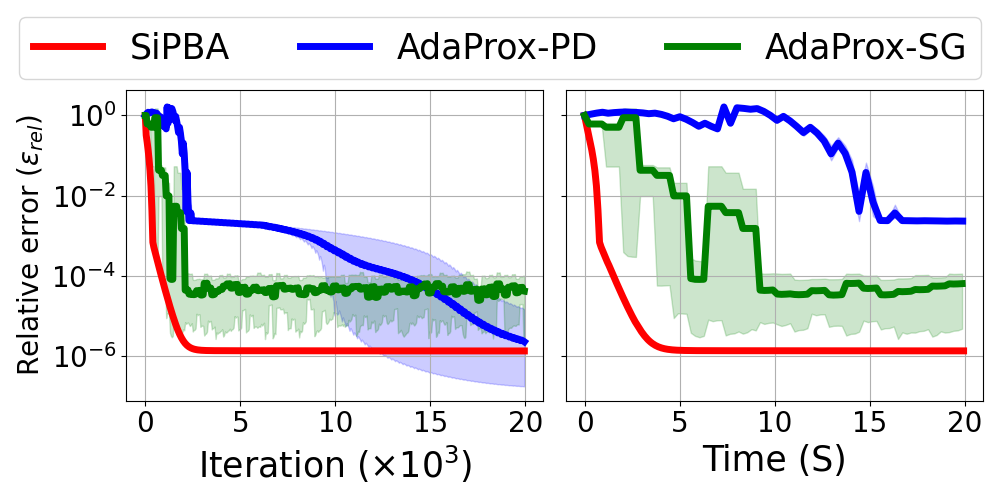
where denotes the all-ones vector of appropriate dimension. For , it can be shown that the unique optimal solution is given by . The performance is assessed by the relative error, . For all experiments in this subsection, the results are averaged over 10 independent runs, each initialized from a distinct, randomly generated starting point. The initial point is generated by sampling each component of from a uniform distribution and each component of from .
| SiPBA | AdaProx-PD | AdaProx-SG | Scholtes-C | Scholtes-D | |
|---|---|---|---|---|---|
| Min. | |||||
| Max. | 0.10 | 1.06 | |||
| Valid Runs | 10/10 | 10/10 | 9/10 | 1/10 | 1/10 |
| Ave Time (s) | 1.03 | 87.44 | 4.07 | 23.12 | 23.81 |
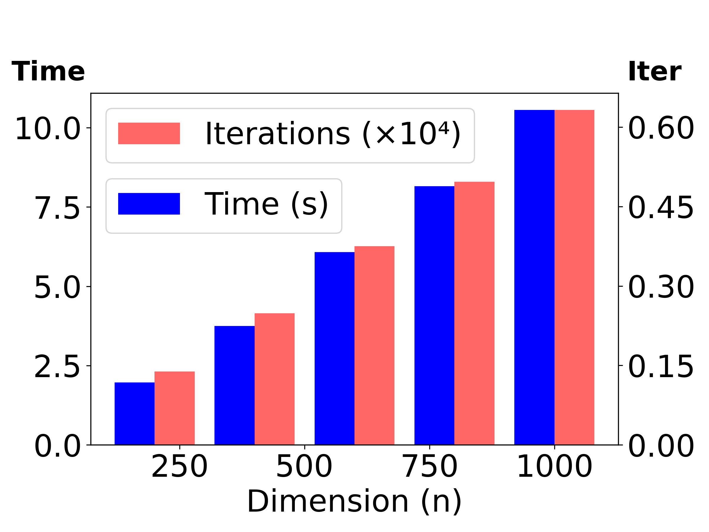
We compare SiPBA against two other gradient-based methods—AdaProx-PD and AdaProx-SG guanadaprox —as well as two MPCC-based approaches— Compact Scholtes (Scholtes-C) and Detailed Scholtes (Scholtes-D) relaxation method benchouk2025scholtes . SiPBA, AdaProx-PD, and AdaProx-SG are run for 20,000 iterations, while Scholtes-C and Scholtes-D are run for 10 outer iterations (as they converge within this range). We report the minimum and maximum relative errors, the number of successful runs achieving the tolerance (Valid Runs), and the average runtime to reach this tolerance for those valid runs (Ave. Time). Figure 1(a) shows the convergence curve of the gradient-based algorithms and Table 1 summarizes the final performance metrics of all the methods. We further evaluate SiPBA’s robustness to hyperparameters (stepsizes and update factors ) and its scalability by measuring runtime and iterations required to achieve the tolerance, , across varying hyperparameters and problem dimensions, with results shown in Table 5.1 and Figure 1 (b). All the results indicate the consistent performance and computational efficiency of SiPBA.
tableAblation analysis for SiPBA on (16) with . Time (s) 0.1 0.001 0.001 0.001 0.1 1.0 1 0.001 0.001 0.001 0.1 0.1 0.01 0.001 0.001 0.001 0.1 14.5 0.1 0.01 0.001 0.001 0.1 0.5 0.1 0.0001 0.001 0.001 0.1 16.4 0.1 0.001 0.01 0.001 0.1 1.4 Time (s) 0.1 0.001 0.0001 0.001 0.1 1.0 0.1 0.001 0.001 0.01 0.1 1.2 0.1 0.001 0.001 0.0001 0.1 1.1 0.1 0.001 0.001 0.001 0.3 5.0 0.1 0.001 0.001 0.001 0.016 0.8 0.1 0.001 0.01 0.01 0.16 1.9
5.2 Spam classification
Spam classification is challenging due to adversarial dynamics and poor cross-domain generalization. We consider the PBO model for spam classification tasks, as proposed by bruckner2011stackelberg :
| (17) |
where denotes the classifier parameters, represents vectorized training data, (resp. ) corresponds to the classifier (resp. adversarial generator) loss, denotes the regularization term, and characterizes the feature of data.
We conduct a two-part empirical comparison. First, we compare the PBO model (17) trained using SiPBA (with as the top principal components) to the same model trained using the SQP method with , as proposed in bruckner2011stackelberg . Second, we compare the SiPBA-trained PBO model against a standard single-level model, , trained using the scikit-learn library pedregosa2011scikit . We use either hinge loss or cross-entropy for both and , and refer to the resulting methods as SiPBA-Hinge/CE, SQP-Hinge/CE, and Single-Hinge/CE.
Experiments are conducted using four standard spam datasets: TREC2006 ounis2006overview , TREC2007 macdonald2007overview , EnronSpam metsis2006spam , and LingSpam androutsopoulos2000evaluation . The average results over ten independent runs are summarized in Table 2, which indicate that the PBO model (either trained with SQP or SiPBA) exhibits superior cross-domain performance compared to the single-level models. Moreover, the SiPBA-trained models achieve the best overall accuracy and F1 score.
| Train Set | Model | Test Set(Acc/F1) | Ave(Acc/F1) | |||
|---|---|---|---|---|---|---|
| TREC06 | TREC07 | EnronSpam | LingSpam | |||
| TREC06 | SiPBA-Hinge | 96.4/94.7 | 87.3/81.0 | 70.6/70.2 | 87.6/92.7 | 85.5/84.7 |
| SiPBA-CE | 94.5/92.5 | 79.5/73.0 | 70.9/71.8 | 87.6/92.8 | 83.1/82.5 | |
| SQP-Hinge | 93.1/90.0 | 89.2/83.2 | 69.0/66.7 | 89.0/93.4 | 85.1/83.3 | |
| SQP-CE | 93.6/91.3 | 78.9/72.4 | 70.7/71.4 | 87.2/92.6 | 82.6/81.9 | |
| Single-Hinge | 95.4/93.1 | 89.3/82.8 | 63.9/46.5 | 75.5/82.5 | 81.0/76.2 | |
| Single-CE | 93.8/90.4 | 88.5/79.6 | 56.9/24.1 | 55.1/62.6 | 73.6/64.2 | |
| TREC07 | SiPBA-Hinge | 68.9/16.8 | 93.7/89.7 | 57.0/33.7 | 50.5/57.6 | 67.5/49.5 |
| SiPBA-CE | 71.7/56.9 | 98.1/97.2 | 68.3/68.8 | 64.6/75.5 | 75.7/74.6 | |
| SQP-Hinge | 68.9/17.2 | 95.3/92.5 | 55.0/21.0 | 29.9/28.1 | 62.3/39.7 | |
| SQP-CE | 71.3/56.9 | 97.7/96.6 | 68.4/69.7 | 70.1/80.5 | 76.9/75.9 | |
| Single-Hinge | 65.4/1.9 | 97.7/96.4 | 50.9/0.2 | 16.6/0.3 | 57.7/24.7 | |
| Single-CE | 66.4/3.4 | 95.7/93.0 | 51.0/0.8 | 17.3/1.8 | 57.6/24.8 | |
| EnronSpam | SiPBA-Hinge | 75.8/61.8 | 72.1/28.0 | 95.9/95.8 | 59.6/67.4 | 75.9/63.3 |
| SiPBA-CE | 76.3/62.8 | 74.0/34.4 | 95.2/95.0 | 64.0/72.0 | 77.4/66.1 | |
| SQP-Hinge | 77.5/61.7 | 70.5/22.8 | 96.1/96.0 | 52.3/59.3 | 74.1/60.0 | |
| SQP-CE | 76.0/62.6 | 73.4/32.9 | 94.9/94.8 | 63.0/71.0 | 76.8/65.3 | |
| Single-Hinge | 76.8/56.0 | 69.3/15.0 | 95.8/95.6 | 47.2/52.3 | 72.3/54.7 | |
| Single-CE | 76.4/55.4 | 70.0/19.2 | 95.6/95.3 | 43.1/46.9 | 71.3/54.2 | |
| LingSpam | SiPBA-Hinge | 63.4/59.1 | 66.2/51.2 | 71.1/65.4 | 99.4/99.6 | 75.0/68.8 |
| SiPBA-CE | 71.8/48.5 | 69.0/27.6 | 59.1/34.3 | 91.8/94.8 | 72.9/51.3 | |
| SQP-Hinge | 42.5/53.8 | 45.3/52.0 | 72.5/65.8 | 98.2/99.0 | 64.6/67.7 | |
| SQP-CE | 72.0/49.5 | 68.9/26.2 | 58.9/33.9 | 91.9/94.8 | 72.9/51.1 | |
| Single-Hinge | 37.2/51.9 | 38.6/50.6 | 56.7/69.0 | 95.7/97.5 | 57.1/67.3 | |
| Single-CE | 34.5/51.0 | 34.0/50.1 | 51.3/66.8 | 91.4/95.1 | 52.8/65.8 | |
5.3 Hyper-representation
Hyper-representationgrazzi2020iteration ; franceschi2018bilevel aim to learn an effective representation of the input data for lower-level classifiers, where PBO model was used to handle the potential multiplicity of optimal solutions in the lower-level problem and robust learn the representation guanadaprox . In this experiment, we further explore the potential of the PBO model and compare it with optimistic models.
5.3.1 Linear hyper-representation on synthetic data
We begin with a synthetic linear hyper-representation task, which is formulated as:
| (18) |
where and are the validation and training feature matrices, and are the corresponding response vectors. The synthetic data is generated as in grazzi2020iteration , with feature matrices and ground-truth matrices and vectors sampled randomly. The response vectors are formed using the linear model , with Gaussian noise added to both and for train and valid data to simulate noise.
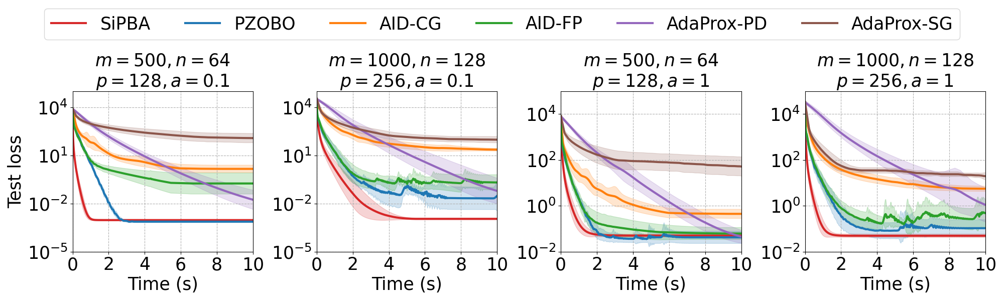
To evaluate solver efficiency and formulation effectiveness, we conduct a two-part comparison. First, we compare the SiPBA algorithm with PBO algorithms AdaProx-PD and AdaProx-SG. Second, we assess the impact of the bilevel formulation by comparing the pessimistic model (18) (solved by SiPBA) with its optimistic variant (solved by AID-FP , AID-CG grazzi2020iteration and PZOBO sow2022convergence ), which replaces with in the upper level. To assess the robustness of each method under varying levels of noise, we conduct experiments with moderate () and severe () perturbations. The performance is measured by test loss, averaged over 10 random seeds. Results in Figure 2 demonstrate the stability and efficiency of SiPBA.
5.3.2 Deep hyper-representation on MNIST and FashionMNIST
To further assess the practical effectiveness of the pessimistic model, we conduct a more complicated deep hyper-representation experiment on real-world classification tasks. The problem is formulated as:
| (19) |
where represents a neural network parameterized by , and corresponds to a linear layer.
We adopt the LeNet-5 architecture sow2022convergence as the feature extractor and evaluate performance on the MNIST and FashionMNIST datasets. Each dataset is randomly split into 50,000 training samples, 10,000 validation samples, and 10,000 test samples, with performance evaluated by test accuracy. We compare the pessimistic formulation (19), trained with SiPBA, to its optimistic variant (replacing with in the upper level) trained with AID-FP, AID-CG grazzi2020iteration , and PZOBO sow2022convergence . Mean results over ten runs are shown in Figure 3, which shows that SiPBA achieves the highest test accuracy.

6 Conclusions and future work
This paper introduces a novel smooth approximation for PBO, which underpins the development of SiPBA, an efficient new gradient-based PBO algorithm. SiPBA avoids computationally expensive second-order derivatives and the need for iterative inner-loop procedures to solve subproblems.
The current study is confined to deterministic PBO problems. However, a significant number of practical applications feature PBO problems within stochastic settings. Extending the SiPBA methodology to effectively address these stochastic PBO problems presents a crucial and promising direction for future research. We hope this research stimulates further algorithmic development for stochastic PBO.
Acknowledgements
Authors listed in alphabetical order. This work was supported by National Key R&D Program of China (2023YFA1011400), National Natural Science Foundation of China (12222106, 12326605), Guangdong Basic and Applied Basic Research Foundation (No. 2022B1515020082), the Longhua District Science and Innovation Commission Project Grants of Shenzhen (Grant No.20250113G43468522) and Natural Science Foundation of Shenzhen (20250530150024003).
References
- [1] A. Aboussoror and P. Loridan. Existence of solutions to two-level optimization problems with nonunique lower-level solutions. Journal of Mathematical Analysis and Applications, 254(2):348–357, 2001.
- [2] A. Aboussoror and A. Mansouri. Weak linear bilevel programming problems: existence of solutions via a penalty method. Journal of Mathematical Analysis and Applications, 304(1):399–408, 2005.
- [3] E. Alekseeva, Y. Kochetov, and E.-G. Talbi. A matheuristic for the discrete bilevel problem with multiple objectives at the lower level. International Transactions in Operational Research, 24(5):959–981, 2017.
- [4] G. B. Allende and G. Still. Solving bilevel programs with the KKT-approach. Mathematical Programming, 138:309–332, 2013.
- [5] M. J. Alves and C. H. Antunes. A semivectorial bilevel programming approach to optimize electricity dynamic time-of-use retail pricing. Computers & Operations Research, 92:130–144, 2018.
- [6] I. Androutsopoulos, J. Koutsias, K. V. Chandrinos, G. Paliouras, and C. D. Spyropoulos. An evaluation of naive Bayesian anti-spam filtering. In Workshop on Machine Learning in the New Information Age, 2000.
- [7] M. Arbel and J. Mairal. Amortized implicit differentiation for stochastic bilevel optimization. In International Conference on Learning Representations, 2022.
- [8] D. Aussel and A. Svensson. Is pessimistic bilevel programming a special case of a mathematical program with complementarity constraints? Journal of Optimization Theory and Applications, 181:504–520, 2019.
- [9] X. Ban, S. Lu, M. Ferris, and H. X. Liu. Risk averse second best toll pricing. In Transportation and Traffic Theory 2009: Golden Jubilee: Papers selected for presentation at ISTTT18, a peer reviewed series since 1959, pages 197–218. Springer, 2009.
- [10] A. Beck. First-order methods in optimization. SIAM, 2017.
- [11] I. Benchouk, L. O. Jolaoso, K. Nachi, and A. B. Zemkoho. Relaxation methods for pessimistic bilevel optimization. arXiv preprint arXiv:2412.11416, 2024.
- [12] I. Benchouk, L. O. Jolaoso, K. Nachi, and A. B. Zemkoho. Scholtes relaxation method for pessimistic bilevel optimization. Set-Valued and Variational Analysis, 33(2):10, 2025.
- [13] D. Benfield, S. Coniglio, M. Kunc, P. T. Vuong, and A. Zemkoho. Classification under strategic adversary manipulation using pessimistic bilevel optimisation. arXiv preprint arXiv:2410.20284, 2024.
- [14] J. F. Bonnans and A. Shapiro. Perturbation analysis of optimization problems. Springer, 2013.
- [15] L. Bottou, F. E. Curtis, and J. Nocedal. Optimization methods for large-scale machine learning. SIAM Review, 60(2):223–311, 2018.
- [16] M. Brückner and T. Scheffer. Stackelberg games for adversarial prediction problems. In International Conference on Knowledge Discovery and Data Mining, 2011.
- [17] V. Bucarey, S. Calderón, G. Muñoz, and F. Semet. Decision-focused predictions via pessimistic bilevel optimization: A computational study. In Integration of Constraint Programming, Artificial Intelligence, and Operations Research, 2024.
- [18] H. I. Calvete, C. Galé, A. Hernández, and J. A. Iranzo. A novel approach to pessimistic bilevel problems. an application to the rank pricing problem with ties. Optimization, pages 1–34, 2024.
- [19] B. Colson, P. Marcotte, and G. Savard. An overview of bilevel optimization. Annals of Operations Research, 153:235–256, 2007.
- [20] S. Dempe, B. S. Mordukhovich, and A. B. Zemkoho. Necessary optimality conditions in pessimistic bilevel programming. Optimization, 63(4):505–533, 2014.
- [21] S. Dempe, B. S. Mordukhovich, and A. B. Zemkoho. Two-level value function approach to non-smooth optimistic and pessimistic bilevel programs. Optimization, 68(2-3):433–455, 2019.
- [22] S. Dempe and A. B. Zemkoho. The bilevel programming problem: reformulations, constraint qualifications and optimality conditions. Mathematical Programming, 138:447–473, 2013.
- [23] S. Dempe and A. B. Zemkoho. Bilevel optimization. In Springer Optimization and its Applications, volume 161. Springer, 2020.
- [24] F. Facchinei and J.-S. Pang. Finite-dimensional variational inequalities and complementarity problems. Springer, 2003.
- [25] L. Franceschi, M. Donini, P. Frasconi, and M. Pontil. A bridge between hyperparameter optimization and learning-to-learn. In Advances in Neural Information Processing Systems, 2017.
- [26] L. Franceschi, M. Donini, P. Frasconi, and M. Pontil. Forward and reverse gradient-based hyperparameter optimization. In International Conference on Machine Learning, 2017.
- [27] L. Franceschi, P. Frasconi, S. Salzo, R. Grazzi, and M. Pontil. Bilevel programming for hyperparameter optimization and meta-learning. In International Conference on Machine Learning, 2018.
- [28] K. Gao and O. Sener. Modeling and optimization trade-off in meta-learning. In Advances in Neural Information Processing Systems, volume 33, pages 11154–11165, 2020.
- [29] R. Grazzi, L. Franceschi, M. Pontil, and S. Salzo. On the iteration complexity of hypergradient computation. In International Conference on Machine Learning, 2020.
- [30] A. Gu, S. Lu, P. Ram, and L. Weng. Nonconvex min-max bilevel optimization for task robust meta learning. In International Conference on Machine Learning, 2021.
- [31] Z. Guan, D. Sow, S. Lin, and Y. Liang. Adaprox: A novel method for bilevel optimization under pessimistic framework. In Conference on Parsimony and Learning, 2025.
- [32] L. Guo, J. J. Ye, and J. Zhang. Sensitivity analysis of the maximal value function with applications in nonconvex minimax programs. Mathematics of Operations Research, 49(1):536–556, 2024.
- [33] M. Hong, H.-T. Wai, Z. Wang, and Z. Yang. A two-timescale stochastic algorithm framework for bilevel optimization: Complexity analysis and application to actor-critic. SIAM Journal on Optimization, 33(1):147–180, 2023.
- [34] Q. Hu, B. Wang, and T. Yang. A stochastic momentum method for min-max bilevel optimization. In Workshop on Optimization for Machine Learning, 2021.
- [35] K. Ji, J. Yang, and Y. Liang. Bilevel optimization: Convergence analysis and enhanced design. In International Conference on Machine Learning, 2021.
- [36] D. Jiménez, B. K. Pagnoncelli, and H. Yaman. Pessimistic bilevel optimization approach for decision-focused learning. arXiv preprint arXiv:2501.16826, 2025.
- [37] T. Kis, A. Kovács, and C. Mészáros. On optimistic and pessimistic bilevel optimization models for demand response management. Energies, 14(8):2095, 2021.
- [38] J. Kwon, D. Kwon, S. J. Wright, and R. D. Nowak. A fully first-order method for stochastic bilevel optimization. In International Conference on Machine Learning, 2023.
- [39] J. Kwon, D. Kwon, S. J. Wright, and R. D. Nowak. On penalty methods for nonconvex bilevel optimization and first-order stochastic approximation. In International Conference on Learning Representations, 2024.
- [40] L. Lampariello, S. Sagratella, and O. Stein. The standard pessimistic bilevel problem. SIAM Journal on Optimization, 29(2):1634–1656, 2019.
- [41] Z. Lin, H. Li, and C. Fang. Accelerated Optimization for Machine Learning. Springer, 2020.
- [42] B. Liu, M. Ye, S. J. Wright, P. Stone, and Q. Liu. Bome! bilevel optimization made easy: A simple first-order approach. In Advances in Neural Information Processing Systems, 2022.
- [43] J. Liu, Y. Fan, Z. Chen, and Y. Zheng. Pessimistic bilevel optimization: A survey. International Journal of Computational Intelligence Systems, 11(1):725–736, 2018.
- [44] R. Liu, Y. Liu, S. Zeng, and J. Zhang. Towards gradient-based bilevel optimization with non-convex followers and beyond. In Advances in Neural Information Processing Systems, 2021.
- [45] R. Liu, Z. Liu, W. Yao, S. Zeng, and J. Zhang. Moreau envelope for nonconvex bi-level optimization: A single-loop and hessian-free solution strategy. In International Conference on Machine Learning, 2024.
- [46] R. Liu, P. Mu, X. Yuan, S. Zeng, and J. Zhang. A generic first-order algorithmic framework for bi-level programming beyond lower-level singleton. In International Conference on Machine Learning, 2020.
- [47] P. Loridan and J. Morgan. Approximate solutions for two-level optimization problems. In French-German Conference on Optimization. Springer, 1988.
- [48] J. Lorraine, P. Vicol, and D. Duvenaud. Optimizing millions of hyperparameters by implicit differentiation. In International Conference on Artificial Intelligence and Statistics, 2020.
- [49] S. Lu. Slm: A smoothed first-order lagrangian method for structured constrained nonconvex optimization. In Advances in Neural Information Processing Systems, 2023.
- [50] Z. Lu and S. Mei. First-order penalty methods for bilevel optimization. SIAM Journal on Optimization, 34(2):1937–1969, 2024.
- [51] Z.-Q. Luo, J.-S. Pang, and D. Ralph. Mathematical programs with equilibrium constraints. Cambridge University Press, 1996.
- [52] C. Macdonald, I. Ounis, and I. Soboroff. Overview of the TREC 2007 blog track. In Text REtrieval Conference, 2007.
- [53] D. Maclaurin, D. Duvenaud, and R. P. Adams. Gradient-based hyperparameter optimization through reversible learning. In International conference on Machine Learning, 2015.
- [54] V. Metsis, I. Androutsopoulos, and G. Paliouras. Spam filtering with naive Bayes-which naive Bayes? In CEAS, volume 17, pages 28–69. Mountain View, CA, 2006.
- [55] B. S. Mordukhovich. Variational Analysis and Applications. Springer, 2018.
- [56] I. Ounis, C. Macdonald, and I. Soboroff. Overview of the TREC 2006 blog track. In Text REtrieval Conference, 2006.
- [57] J. V. Outrata. On the numerical solution of a class of stackelberg problems. Zeitschrift für Operations Research, 34(4):255–277, 1990.
- [58] F. Pedregosa. Hyperparameter optimization with approximate gradient. In International Conference on Machine Learning, 2016.
- [59] F. Pedregosa, G. Varoquaux, A. Gramfort, V. Michel, B. Thirion, O. Grisel, M. Blondel, P. Prettenhofer, R. Weiss, and V. Dubourg. Scikit-learn: Machine learning in python. the Journal of Machine Learning Research, 12:2825–2830, 2011.
- [60] R. T. Rockafellar and R. J.-B. Wets. Variational Analysis, volume 317. Springer, 2009.
- [61] H. Shen and T. Chen. On penalty-based bilevel gradient descent method. In International Conference on Machine Learning, 2023.
- [62] D. Sow, K. Ji, and Y. Liang. On the convergence theory for hessian-free bilevel algorithms. In Advances in Neural Information Processing Systems, 2022.
- [63] S. Sra, S. Nowozin, and S. J. Wright. Optimization for Machine Learning. MIT Press, 2011.
- [64] M. A. Ustun, L. Xu, B. Zeng, and X. Qian. Hyperparameter tuning through pessimistic bilevel optimization. arXiv preprint arXiv:2412.03666, 2024.
- [65] P. Virtanen, R. Gommers, T. E. Oliphant, M. Haberland, T. Reddy, D. Cournapeau, E. Burovski, P. Peterson, W. Weckesser, J. Bright, et al. Scipy 1.0: fundamental algorithms for scientific computing in python. Nature methods, 17(3):261–272, 2020.
- [66] H. von. Stackelberg. The Theory of the Market Economy. Oxford University Press, 1952.
- [67] W. Wiesemann, A. Tsoukalas, P.-M. Kleniati, and B. Rustem. Pessimistic bilevel optimization. SIAM Journal on Optimization, 23(1):353–380, 2013.
- [68] Y. Yang, Z. Si, S. Lyu, and K. Ji. First-order minimax bilevel optimization. In Advances in Neural Information Processing Systems, 2024.
- [69] W. Yao, C. Yu, S. Zeng, and J. Zhang. Constrained bi-level optimization: Proximal lagrangian value function approach and hessian-free algorithm. In International Conference on Learning Representations, 2024.
- [70] J. J. Ye and D. L. Zhu. Optimality conditions for bilevel programming problems. Optimization, 33(1):9–27, 1995.
- [71] B. Zeng. A practical scheme to compute the pessimistic bilevel optimization problem. INFORMS Journal on Computing, 32(4):1128–1142, 2020.
- [72] Y. Zhang, G. Zhang, P. Khanduri, M. Hong, S. Chang, and S. Liu. Revisiting and advancing fast adversarial training through the lens of bi-level optimization. In International Conference on Machine Learning, 2022.
- [73] Y. Zheng, Z. Wan, K. Sun, and T. Zhang. An exact penalty method for weak linear bilevel programming problem. Journal of Applied Mathematics and Computing, 42(1):41–49, 2013.
- [74] Y. Zheng, G. Zhang, J. Han, and J. Lu. Pessimistic bilevel optimization model for risk-averse production-distribution planning. Information Sciences, 372:677–689, 2016.
- [75] Z. Zheng and S. Gu. Safe multi-agent reinforcement learning with bilevel optimization in autonomous driving. IEEE Transactions on Artificial Intelligence, 6(4):829–842, 2025.
Appendix A Numerical experiment
In this section, we provide the specific description of experiments in Section 5. All experiments were conducted on CPUs except for the spam classification task, which utilized an NVIDIA H100 GPU. The primary compute node features dual Intel Xeon Gold 5218R processors operating at 2.1GHz base frequency (4.0GHz turbo boost), featuring 40 physical cores (80 logical threads) with a three-tier cache architecture: 1.3MB L1, 40MB L2, and 55MB L3 shared cache. The NUMA-based memory architecture partitions resources across two distinct domains, with hardware support for AVX-512 vector instructions and VT-x virtualization. Security mitigations against Spectre/Meltdown vulnerabilities were implemented through combined microcode patches and kernel-level protections.
A.1 Synthetic example
For the problem 5.1, we can get the value function by simple calculation:
| (20) |
which implies that . Except for the stability tests of the initial step sizes reported in Table 5.1, we fix the hyper-parameters as
| (21) |
For the implementation of AdaProx-PD, we first fix , , , , and set , , , and , . Then we perform a grid search for
However, none of these yielded satisfactory convergence. We thus fixed parameters across iterations, set , , , , , and conducted a grid search to find a best parameter to get lowest loss, where the grid is set as follows:
As a result, we have , , , and for AdaProx-PD.
For the implementation of AdaProx-SG, we fix , , and , and , . Then we perform a grid search for
As a result, we have , , and for AdaProx-SG.
A.2 Spam classification
Spam classification remains a critical challenge in machine learning due to adversarial dynamics: spammers adapt their strategies in response to deployed classifiers, while models trained on specific datasets often exhibit poor cross-domain generalization. In this paper, we extend the pessimistic bilevel model for Spam classification in [16]:
| (22) |
where denotes the classifier parameters, represents vectorized training data, (resp. ) corresponds to the classifier (resp. adversarial generator) loss, denotes the regularization term, and characterizes the feature of data. This framework explicitly models spammer adaptations through adversarial samples , enhancing classifier robustness against evolving threats.
We evaluate our model on four benchmark datasets:
-
•
TREC06 (37,822 emails; 24,912 spam / 12,910 ham): https://plg.uwaterloo.ca/cgi-bin/cgiwrap/gvcormac/foo06
-
•
TREC07 (75,419 emails; 50,199 spam / 25,220 ham): https://plg.uwaterloo.ca/cgi-bin/cgiwrap/gvcormac/foo07
-
•
EnronSpam (33,715 emails; 16,545 spam / 17,170 ham): https://www.cs.cmu.edu/˜enron/
-
•
LingSpam (2,893 emails; 481 spam / 2,412 ham): https://www.aueb.gr/users/ion/data/lingspam_public.tar.gz
The text was vectorized using a TfidfVectorizer that removed English stop words, retained only terms appearing in at least five documents, and limited the feature space to the top 9000 most informative terms. We represent the resulting vectors as the variable and train the model in the vectorized space. To simulate the real world situation, we assume that email authors always aim to have their messages classified as ham; accordingly, we define as the loss incurred when an email is classified as spam, using the same formulation (cross‐entropy or hinge) as . The specific definition of and used in our experiment is given by
where denotes the input data, denotes the label (-1 for spam and 1 for non-spam) and CrossEntropy is defined by and is the Sigmoid function. The function is defined as
where the matrix consists of the top principal components obtained from the principal component decomposition of the sample matrix. This choice is motivated by the assumption that meaningful information in emails is primarily captured by the principal components, and modifications made by spammers generally do not alter this core content. Therefore, we penalize changes along the principal components to enforce robustness against adversarial modifications. In this experiment, we always set for SiPBA.
For the implementation of SiPBA, we fix , , , and , and we set the hyperparameter as follows:
| TREC06: | |||
| TREC07: | |||
| EnronSpam: | |||
| LingSpam: |
For the implementation of SQP-Hinge and SQP-CE, we set (to ensure the lower level can be uniquely solved) and and solve the problem using the trust-constr method from the scipy.optimize solver [65].
For the implementation of Single-Hinge and Single-CE, we use SVC and Logistic Regression from scikit-learn [59] with default setting and .
A.3 Hyper-representation
In the linear hyper-representation on synthetic data, we follow the data generation procedure of [62]. Specifically, we generate the ground‐truth matrix , the vector , and the inputs by sampling each entry independently from the standard normal distribution . We then generate the train, valid and test data by Finally, we add with and to and to simulate the noise condition. The parameters of the algorithms are initialized as
-
•
For SiPBA, we set And the stepsize is set as for and for the remaining senarios.
-
•
For AdaProx-PD, we set , , , , and , and . And the stepsize is setted as for the four senarios in Figure 2.
-
•
For AdaProx-SG, we set , , , , , , and .
-
•
For AID‐FP, AID‐CG and PZOBO, we keep the setting as presented in https://github.com/sowmaster/esjacobians/tree/master, except that the inner learning rate is set as as we found it’s more stable for these algorithms.
For the classification tasks on MNIST and FashionMNIST, we split the dataset into 50,000 training samples, 10,000 validation samples, and 10,000 test samples. Both the upper and lower levels are trained using the LeNet architecture, following the setting in [62]. During each training iteration, we randomly select 256 samples to compute the loss and gradients. The parameters of the algorithms are initialized as follows:
-
•
For SiPBA, we set and
-
•
For PZOBO, we adopt the implementations from https://github.com/sowmaster/esjacobians/tree/master and set number of inner iterations for training on FashionMNIST to ensure proper convergence.
-
•
For AID-CG, we set the learning rate to and the number of inner iterations to for training on MNIST (FashionMNIST).
-
•
For AID-FP, we set and for training on MNIST (FashionMNIST) .
A.4 Parameter Selection
The implementation of SiPBA includes seven parameters, namely . The parameters , , and collectively govern the fundamental trade-off between value function approximation accuracy and iterative step size selection. The parameter controls the growth rate of the penalty coefficient , while determines the decay rate of the regularization coefficient . Larger values of and yield faster convergence of the approximate value function to the true objective. The parameter regulates the step size decay rate for the primal iterates .
The theoretical requirement reveals an essential trade-off: choosing larger values for and accelerates the value function approximation but necessitates a larger , resulting in smaller step sizes that slows down the convergence rate of . Conversely, smaller and permit more aggressive step sizes through reduced , but at the cost of slower convergence of the approximate objective to the true value function, potentially degrading overall algorithmic performance.
We provide practical guidelines for parameter selection here. Specifically, the update rules are given by:
with default settings and . Therefore, tuning is only required for the three scalar parameters: , , and .
Appendix B Proofs for Section 2
This section provides the proofs for the theoretical results established in Section 2.
B.1 Equivalent minimax reformulation of
Lemma B.1
Consider the function
where
Then, for any , we have the following equivalent minimax reformulation:
Let be an arbitrary point. The assumptions that is nonempty, and is -strongly concave with respect to , and using the fact that is closed, we conclude that there exists some such that .
For any , since , it follows that
Therefore, we have
Taking the minimum over all , we obtain
Next, we establish the reverse inequality. Consider the specific choice , since , we have
Thus, we conclude that
This completes the proof.
B.2 Proof for Theorem 2.1
The proof strategy is analogous to that employed in [69, Lemma A.1]. We proceed by first analyzing an auxiliary function and then leveraging its properties to establish the differentiability of .
Let us define an auxiliary function as:
By assumption, is continuous differentiable on , and is -strongly convex with respect to for any .
The -strongly convexity of with respect to ensures the uniqueness of the minimizer of (equivalently, the maximizer of ). Let us denote this unique maximizer as . Furthermore, it can be shown that satisfies the inf-compactness condition as stated in [14, Theorem 4.13] on any point . Specifically, for any , there exists a constant , a compact set , and a neighborhood of such that the level set is nonempty and contained in for all . Given that is continuously differentiable, is unique, and the inf-compactness condition holds, we can apply [14, Theorem 4.13, Remark 4.14]. This theorem implies that is differentiable on , and its gradient is given by:
| (23) |
The strong concavity of in and the continuous differentiability of imply that is continuous on . Since and are continuous by assumption, and is continuous, it follows from (23) that is continuous on . Thus, is continuously differentiable on .
The function can be expressed using as:
| (24) |
We are given that is -strongly convex with respect to for any fixed . Since , and the maximum of a set of functions preserves strong convexity (see, e.g., [10, Theorem 2.16]), it can be shown that is -strongly convex with respect to for any fixed . The -strong convexity of with respect to ensures the uniqueness of the minimizer . This strong convexity, combined with the established continuous differentiability (and thus continuity) of , ensures that satisfies the inf-compactness condition for for any . Furthermore, is continuous on .
We can again apply [14, Theorem 4.13, Remark 4.14] to . The conditions are met: is continuously differentiable (as shown above), and is unique. Therefore, is differentiable on , and its gradient is given by:
where denotes . Since is continuous on , is continuous on and is continuous on , the composite function is continuous on . Thus, is continuously differentiable.
Additionally, because is strongly concave in and strongly convex in for any , and because for any , it follows that for any . Thus, the desired conclusion is obtained.
B.3 Proof for Lemma 2.2
Before presenting the proof for Lemma 2.2, we first establish some auxiliary results. Throughout this subsection, given sequences and , we will use the shorthand notations , , and to denote , , and , respectively, for notational brevity.
First, we establish a uniform boundedness property for the saddle point components and .
Lemma B.2
Let and be sequences such that and as . Let be a compact set. Then, there exists a constant such that for all and all ,
where is the unique saddle point of the minimax problem .
The proof proceeds in two parts, establishing the boundedness of and separately, both by contradiction.
Suppose, for the sake of contradiction, that is not uniformly bounded. Then there exists a sequence such that as .
By Assumption 2, for each , there exits such that , where is a compact set. Thus, the sequences and are uniformly bounded. Since is continuous differentiable on and is -strongly concave in for any , and , we have
| (25) |
Next, since , we know that . Given , it follows that:
From (25), we deduce:
| (26) |
By the saddle point property of :
Combining this with (26) yields:
| (27) |
Since , we have . Thus:
Since and are bounded, and is continuous on , is bounded. As , the term is bounded below. This contradicts (27). Therefore, our initial assumption was false, and there must exist such that for all and .
Next, we show that there exists such that for any and . Suppose, for the sake of contradiction, that is not uniformly bounded. Then there exists sequence such that as . By Assumption 2, for each , there exists for a compact set , so is bounded.
From the saddle point property, minimizes over . Thus:
Expanding this inequality, simplifying and rearranging terms:
Combining the above inequality with the fact that yields that:
| (28) |
The right-hand side of (28) is bounded because and are bounded. However, since and is bounded, the left-hand side . This presents a contradiction. Thus, our assumption was false, and there exists such that for any and , .
Next, we demonstrate that accumulation points of belong to the solution set when .
Lemma B.3
Let and be sequences such that and as . Then, for any sequence such that as , we have
| (29) |
Consequently, for any accumulation point of sequence , we have .
Let be an arbitrary point in . From the saddle point property, maximizes over . Thus:
Expanding this inequality:
Rearranging this inequality to isolate terms involving , and since , we can divide by :
By Lemma B.2, and are uniformly bounded. Since is continuous on and converges, and are bounded. Given and , the entire right-hand side of the inequality converges to as . Therefore, by taking in the above inequality, and since is continuous on , we have
This concludes the proof.
We prove the first statement (i.e., ) by contradiction. Suppose there exist and such that
Then, by properties of , there exists a subsequence (which we re-index by for simplicity) such that
Recall that is the saddle point for the minimax problem . Thus, . Expanding , we have:
| (30) |
By Lemma B.2, is bounded. Thus, we can extract a further subsequence (again re-indexed by ) such that for some . By Lemma B.3, this implies .
From the saddle point property, minimizes over . Therefore,
Expanding this:
Rearranging:
Combing this with (30) yields that
Taking in the above inequality, since is continuous on , we have
However, since , by the definition , we must have . This leads to . Since , this is a contradiction. Therefore, the initial assumption was false, and we must have
The second conclusion then follows from this result and the Proposition 7.30 in [60].
B.4 Proof for Proposition 2.3
For any given , Assumption 2 ensures that the set is nonempty and closed. Combined with the -strong concavity of with respect to , this guarantees the existence of a unique maximizer such that , i.e., .
We first establish a uniform boundedness property for when is restricted to a compact set.
Lemma B.4
Let be a compact set in . Then, there exists a constant such that for any ,
where .
Suppose, for the sake of contradiction, that such a uniform bound does not exist. Then there must exist a sequence such that as . According to Assumption 2, for each , there exists an element , where is a specified compact set. Consequently, the sequence is uniformly bounded.
Because is continuous differentiable on and is -strongly concave in for any , leading to:
| (31) |
By the definition of as the maximizer of , and since , we have:
Given that from (31), it must also hold that:
However, since both and are bounded, and is continuous on , the sequence must be bounded below. This contradicts the finding that . Thus, our initial assumption must be false, and we get the conclusion.
Next, we establish an inequality relating and .
Lemma B.5
Let be given constants. Then, for any ,
where .
For notational brevity within this proof, let denote . Because is strongly concave in and strongly convex in , we have:
From the max-min formulation, it follows that for any specific choice of , such as ,
| (32) |
Since
to find , we can minimize the terms dependent on :
Since , it follows that
Substituting into :
Combining this with (32), the conclusion follows.
Now, we are ready to provide the proof for Proposition 2.3.
For any and for each , by the definition of infimum, there exists an such that
| (33) |
Applying Lemma B.5 to :
| (34) |
If is bounded, we have that sequence is bounded. Alternatively, if is bounded, Lemma B.4, establishes that is bounded. Under either condition, since as :
Combining this with (33) and (34):
Since was arbitrary, we can let , yielding:
Then the conclusion follows by combining the above inequality with Lemma 2.2.
B.5 Lower semi-continuity of
In this part, we demonstrate that the inner semi-continuity of the lower-level solution set mapping serves as a sufficient condition for the lower semi-continuity of the value function .
We begin by recalling the relevant definitions.
Definition B.6
A function is lower semi-continuous (l.s.c.) at if for any sequence such that as , it holds that
Definition B.7
A set-valued function is inner semi-continuous at if , where .
Lemma B.8
If is inner semi-continuous at , then is lower semi-continuous at .
Let be an arbitrary sequence such that as . If , the inequality hods trivially. Assume . For any , by the definition of supremum, there exists an element such that
Since is inner semi-continuous at , there exists a sequence such that for each , and
Then, by the continuity of and the fact that , we have:
| (35) |
Since this inequality holds for any arbitrary , we can let to conclude:
B.6 Proof for Lemma 2.4
From Lemma B.5, for each , we have the inequality:
| (36) |
where . Since the sequence converges to , it is bounded. By Lemma B.4, the sequence is uniformly bounded. Given that as and is bounded, it follows that
Combing with (36), we obtain
Thus, by the lower semi-continuity of at , we conclude that:
| (37) |
This completes the proof.
B.7 Proof for Theorem 2.6
First, let be a sequence converging to , then we assert that . Assume by contradiction that . Then there exist a such that
Then by the continuity of and convergence of , for sufficiently large ,
which contradicts with . Thus, we have
where . As a result, recalling the definition of the value function , we have
which implies that is upper semi-continuous. Combining the assumption that is lower semi-continuous, we have is continuous. As a result, there exist a sequence such that Since is the saddle point, we have
Recall the definition of and rearrange the items,
where the last equation follows from the boundedness of established in Lemma B.2. Thus, we have any accumulation point of belongs to . Furthermore, by rearranging the items above again,
which implies that . Combining this with the fact that any accumulation point of belongs to , we can conclude that . Furthermore, the saddle point property implies that
By expanding and rearranging the items, we have
Combining this with , the conclusion follows.
Appendix C Proof for Section 4
Throughout this part, we assume Assumption 4, which states that is a bounded set.
Given sequences and , for notational conciseness, we employ the shorthand notations , , and to denote , , and , respectively. We use to denote the pair , and correspondingly, and . The symbols , and denote the normal cones to the sets , and at , and , respectively.
Let and denote the Lipschitz constants of and on , respectively.
Consider the sequences and such that and as . As established in Lemma B.2, the quantity is finite. This implies that the collections of points and are bounded. Given that is bounded, and and its gradient are assumed to be continuous on , the continuity over this effectively bounded domain of evaluation ensures that the suprema and are also finite.
With given sequences and , for each , we define the operator as
By assumption, for any fixed , the function is -strongly convex in and -strongly concave in . Consequently, invoking [60, Theorem 12.17 and Exercise 12.59], it follows that for a fixed , the operator exhibits strong monotonicity with respect to :
| (38) |
Furthermore, under the assumption that the gradients of and are Lipschitz continuous, the operator is also Lipschitz continuous with respect to for any fixed :
| (39) |
C.1 Auxiliary Lemmas
To establish the convergence properties of SiPBA(Algorithm 1), we first introduce several auxiliary lemmas pertaining to the behavior of the iterative sequence. The following lemma demonstrates a contraction property for the sequence .
Lemma C.1
Let and be sequences such that . Define . Suppose the step-size sequence satisfies for each . Let be the sequence generated by SiPBA(Algorithm 1). Then, the iterate and satisfy:
| (40) |
The update rule for can be expressed in the compact form:
Recall that is is the unique saddle point of the minimax problem . From the first-order optimality conditions, satisfies:
which implies
Utilizing the non-expansiveness of the projection operator, the strongly monotonicity of in (38) and its Lipschitz continuity with respect to in (39), we can apply standard results from the analysis of projected fixed-point iterations [24, Theorem 12.1.2]. If the step size , then:
Thus, when , it holds that
The subsequent lemma is dedicated to establishing the Lipschitz continuity of .
Lemma C.2
Let and be sequences such that . Define . Then, for any , the corresponding saddle points and satisfy:
| (41) |
Because and are saddle points to the minimax problem , and , respectively. According to the first-order optimality conditions, these saddle points must satisfy:
| (42) |
and
Next, we analyze the Lipschitz continuity of with respect to . The first component difference is
And the second component difference is
Thus, we obtain
| (43) |
Next, we use the fact that
and apply the strongly monotonicity of from (38), along with the monotonicity of the normal cone and (45). This leads to the following inequality:
By substituting the bound from (43) into the above inequality, we obtain
This completes the proof.
Lemma C.3
Let and be sequences such that , . Define . Then, for any fixed , we have
| (44) |
Because and are saddle points to the minimax problem , and , respectively. According to the first-order optimality conditions, these saddle points satisfy:
| (45) |
and
Next, we expand the differences between the gradients of and at :
and
Thus, we have the following bound for the difference between the operators and :
| (46) |
Now, using the fact that
and combining this with the strongly monotonicity of from (38), the monotonicity of the normal cone and (45), we get
By substituting the bound from (46) into this inequality, we obtain
This completes the proof.
Lemma C.4
Let and be sequences such that . Define . Then, for any , we have
| (47) |
where .
From the expression for given in Theorem 2.1, we have the following:
| (48) | ||||
where the final inequality follows from Lemma C.2.
By synthesizing the results from Lemmas C.1-C.4, the following lemma characterizes the evolution of the squared norm of the tracking error, .
Lemma C.5
Let and be sequences such that , . Define . Suppose the step-size sequence satisfies for each . Let be the sequence generated by SiPBA (Algorithm 1). Then, the following inequality holds:
| (49) | ||||
Using the Cauchy-Schwarz inequality for any , we obtain the following:
| (50) | ||||
Next, take in the above inequality. By applying Lemma C.1, we obtain the following bound:
Using Lemma C.2, we can further bound the second term as follows:
Next, applying Lemma C.3 with , we obtain
Finally, combining the above three inequalities with (50), we arrive at the desired inequality.
Lemma C.6
Let and be sequences such that , . Then, for any , we have
| (51) |
We begin with the expression for as follows:
This leads to the inequality
This completes the proof, as the final inequality is derived from the fact that .
The subsequent lemma characterizes the descent property of the value function across iterations.
Lemma C.7
Let and be sequences such that , . Define . Suppose the step-size sequence satisfies for each . Let be the sequence generated by SiPBA (Algorithm 1). Then, we have
| (52) | ||||
where .
We decompose the total difference as follows:
| (53) |
For the first term, applying Lemma C.6 with :
| (54) |
For the second term, , we use the -Lipschitz continuity of established in Lemma C.4. A standard descent inequality (cf. [10, Lemma 5.7] for smooth functions) states:
| (55) |
Next, applying the update rule for , we get
By combining this inequality with the previous one, and using the formula for given in Theorem 2.1, we obtain
| (56) | ||||
where the last inequality follows from Lemma C.1. The conclusion follows by combining the above inequality with (55) and (54).
Lemma C.8
Let and be sequences such that , and as . Furthermore, assume that is bounded below on , i.e., . Then, there exists a constant such that, for any , we have
Next, by Lemma B.4, we have that there exists such that for all ,
Thus, we can bound the second term in the inequality:
Taking the limit as and using the fact that , we obtain
and then the conclusion follows.
C.2 Proof for Proposition 4.1
Given , and , the constant ratio can be chosen sufficiently small to ensure that for all , the following inequality holds:
Recall the merit function,
Applying Lemmas C.7 and C.5, specifically equations (52) and (49), and using the facts that and , we obtain:
| (58) | ||||
The parameters are set according to the schedules: , , , and . We have that
Since , it follows for sufficiently large that
Therefore,
Furthermore, since , , and , we find that there exists such that
and
Given that , and , we conclude that for sufficiently large :
Substituting this and the earlier bound into (58), we deduce that for large :
| (59) | ||||
Next, we show that the sum of the positive terms on the right-hand side of (59) is bounded. Since and , we have
With , and , there exits such that
which implies
Regarding the remaining terms, since , , , and , there exists such that
Thus, the sum
Similarly, there exists such that
Since , the sum
This completes the proof.
C.3 Proof for Theorem 4.2
The conditions and are chosen to satisfy the requirements of Proposition 4.1. From Proposition 4.1, and noting that for all , we have the following summations:
Rewriting the first sum, we have:
| (60) |
Since the terms in these convergent series are non-negative, it follows that for any :
The parameter schedules are , , , , and . We have
Under the conditions and , we we deduce the convergence rates:
and
Furthermore, the summability in (60) implies
From Theorem 2.1, we have
where the first inequality follows from the nonexpansiveness of the projection operator , and the last inequality follows from Lemma C.1. Since as , and as , it follows that
Furthermore, we have previously shown that:
Combining this with the convergence of the projected gradients yields:
This completes the proof of stationarity.
C.4 Proof for Corollary 4.3
We first establish the following auxiliary result.
Lemma C.9
Assume is lower semi-continuous on . Let and be sequences such that and . Then, for any , there exists such that for all ,
| (61) |
Assume, for the sake of contradiction, that the statement is false. Then there exists an and sequence such that
Since is compact, by passing to a further subsequence if necessary, we can assume . Recall that is the saddle point of the minimax problem . Thus, and by the definition of , we have
| (62) | ||||
By Lemma B.2, the sequence is bounded. Thus, by passing to another subsequence if necessary, we can assume for some . It follows from Lemma B.3 that .
Since is a minimizer of over , we have
Substituting the definition of , this yields:
This simplifies to:
Combining this with (62), we have
Taking the limit as , continuity of and lower semicontinuity of yield
However, since , we must have
leading to a contradiction. Thus, the claim follows.
From Theorem 4.2, we have the stationarity condition:
This condition, together with the Lipschitz continuity of established in Lemma C.4, implies that is an approximate stationary point for . Standard arguments then show that for any , there exists such that for all , there is a such that
According to Lemma B.5, for each :
| (63) |
where . By Lemma B.4, there exists such that for any ,
Since as , we can obtain from (63) that for any , there exists such that for each ,
Furthermore, by Lemma C.9, for any , there exists such that for any ,
Combining these inequalities yields that for any and , we can find such that for each , there exists such that
completing the proof.