Architecture of planetary systems with and without outer giant planets

Understanding the link between outer giant planets (OGPs) and inner light planets (ILPs) is key to understanding planetary system formation and architecture. The correlation between these two populations of planets is debated both theoretically – different formation models predict either a correlation or an anticorrelation – and observationally. Several recent attempts to constrain this correlation have yielded contradictory results, due to small-number statistics and heterogeneous samples. We present an ongoing long-term observational effort with CORALIE, HARPS, and ESPRESSO to probe the ILP occurrence in systems with and without OGP. In this first article of a series, we discuss how, from the design to the observations, we ensured the homogeneity of the samples, both in terms of stellar properties and observing strategy. We also present the first three detections of ILPs in our OGP host sample. We find a $8.3\penalty 10000\ m_{\oplus}$ planet at 5.75 d around HD 23079, a $10.4\penalty 10000\ m_{\oplus}$ planet at 4.6 d around HD 196067, and we confirm the $7.5\penalty 10000\ m_{\oplus}$ planet at 3.98 d around HD 86226. While a rigorous statistical analysis of our samples will be performed in subsequent studies, the relatively low number of detections in our sample seems to contradict previous studies that found a strong OGP-ILP correlation.

1 Introduction

Characterizing the global architecture of planetary systems is crucial for understanding their formation history and dynamical evolution. Although more than 5000 exoplanets have already been detected, it remains extremely challenging to fully characterize both the inner and outer regions of planetary systems due to the disparate planetary orbital periods, ranging from hours to decades, and the detection limits and biases of the different observing methods (transit, radial velocities, imaging, etc.). Thus, the coupling between the inner and outer parts of planetary systems during planet formation and subsequent evolution remains poorly constrained by observations. In particular, the question of whether the presence of outer giant planets (hereafter OGPs) enhances or inhibits the formation of inner light planets (hereafter ILPs) remains open, both theoretically and observationally.

The main planet formation models have different theoretical predictions. In the inward migration theory, in which ILPs are initially formed in the outer part of the protoplanetary disk and migrate to the inner part due to disk-planet interactions, the presence of an OGP is proposed to hinder inward migration (e.g., Izidoro et al. 2015). Similarly, in the pebble accretion theory, ILPs form in the inner part of the disk owing to a flux of pebbles drifting inward from the outer region. The presence of an OGP would, in that case, inhibit the pebble flux and thus the formation of ILPs (e.g., Rice et al. 2006; Ormel et al. 2017; Lambrechts et al. 2019). Thus, these formation models predict an anticorrelation between ILP and OGP populations. However, in the in situ formation model, orbital migration is assumed to play a limited role, and the protoplanetary disk is initially assumed to be sufficiently massive for ILPs to form in the inner region by accretion of solids and gas in their vicinity. Such a massive disk also tends to form gas giant planets in its outer region (e.g., Chiang & Laughlin 2013; Schlecker et al. 2021). Thus, a correlation between ILPs and OGPs would be expected in the in situ formation model.

Several recent studies have attempted to constrain this correlation from observations, leading to contradictory results. Most of these studies rely on comparing the occurrence rates of OGPs in blind radial velocity (RV) surveys and in RV follow-up of transiting ILP hosts. The first attempts (Zhu & Wu 2018; Bryan et al. 2019) find an enhanced probability (by a factor of three, albeit with large uncertainty) of OGP around transiting ILP hosts compared to the general population (OGPs in blind RV surveys). From this, they conclude that stars hosting an OGP have about a 90% chance of also hosting ILPs.

At the same time, a HARPS (High Accuracy Radial velocity Planet Searcher) search for inner planets in 20 OGP hosts(Barbato et al. 2018) yielded no ILP detection. However, the relatively small sample of stars and the low number of HARPS measurements per star (27 on average) did not allow the authors to draw firm conclusions. A statistical analysis of RV archival data from the California Legacy Survey (CLS, Rosenthal et al. 2021), shows a nonsignificant (within 1-$\sigma$) correlation between OGPs and ILPs (Rosenthal et al. 2022). These approaches (Barbato et al. 2018; Rosenthal et al. 2021), as well as the one proposed here, are direct measurements of $P({\rm ILP}|{\rm OGP})$, in contrast to the indirect method proposed by Zhu & Wu (2018); Bryan et al. (2019) which relies on Bayes’ theorem to derive $P({\rm ILP}|{\rm OGP})$ from $P({\rm OGP}|{\rm ILP})$.

More recently, Bonomo et al. (2023) present a dedicated HARPS-N follow-up of 38 transiting ILP hosts to search for OGPs. They report a lower but compatible rate of OGP than in the general population, in contradiction with Zhu & Wu (2018) and Bryan et al. (2019). They attribute this discrepancy to the possible confusion between OGPs and magnetic cycles or binary stars. Another possible reason for this discrepancy, proposed by Zhu (2024), is that the stars observed by Bonomo et al. (2023) are metal-poor compared to the general population. However, the impact of stellar metallicity on the (anti-)correlation between the two populations is still debated (Bryan & Lee 2024; Van Zandt & Petigura 2024; Bryan & Lee 2025; Van Zandt et al. 2025; Bonomo et al. 2025).

More generally, the question of whether these populations correlate or anticorrelate is difficult to settle using archival data. Indeed, all of these studies suffer from small-number statistics (small stellar sample sizes) and/or nonhomogeneous samples, especially when comparing results from blind RV surveys and transit follow-ups. As shown by Van Zandt & Petigura (2024), some results strongly depend on the exact definitions of ILP and OGP (in terms of mass, radius, periods, and semi-major axis). This may partly reflect true physical mechanisms, but could also arise from small-number statistics and biased samples.

Additionally, a subtler issue, which we term “observer-excitement” bias, can affect some of these results. In many blind RV surveys, targets showing promising signals tend to be monitored with higher cadence, while others receive fewer observations. Consequently, blind surveys typically have more RV measurements (sometimes orders of magnitude more) for targets with planets than for those without. This bias can have two relevant effects on OGP-ILP correlations studies:

• Low-amplitude planets are more likely to be detected in multi-planetary systems where an easier-to-detect planet has already been found, increasing the likelihood of intensive monitoring;

• When correcting for completeness, systems with planets typically have more points, and thus lower detection limits, giving them greater weight in occurrence estimates. This typically results in overestimation of occurrence rates.

This observer-excitement bias is very difficult to correct for, especially when combining blind surveys with different observing strategies.

Here, we present a long-term observational effort to study the OGP-ILP (anti-)correlation by probing the ILP occurrence in systems with and without OGP. We constructed two comparative samples of stars, with and without OGP, ensuring the homogeneity of the two samples in terms of stellar properties and observing strategy, to avoid any bias that could affect the comparison. In this first article of a series, we focus on the sample definitions and on the first three detections (two new and one confirmation) of ILP in OGP hosts around HD 23079, HD 196067, and HD 86226, based on the first two years of observations of our program. These three targets were known to host an OGP (see Tinney et al. 2002 for HD 23079, Marmier et al. 2013 for HD 196067, and Arriagada et al. 2010 for HD 86226). Moreover, a transiting ILP has been detected by TESS (Transiting Exoplanet Survey Satellite) and confirmed with follow-up PFS (Planet Finder Spectrograph) RV measurements (Teske et al. 2020) for HD 86226.

In Sect. 2, we present the two samples and the observing strategy. In Sect. 3, we present the properties of the three hosts, and in Sect. 4 we describe the observations. We present our analysis methods in Sect. 5, and our results for the three targets in Sect. 6. Finally, in Sect. 7, we present preliminary conclusions from these detections. A statistical analysis of the full sample to derive the underlying occurrences of ILP with and without OGP will be performed in subsequent articles.

2 Sample definitions and observing strategy

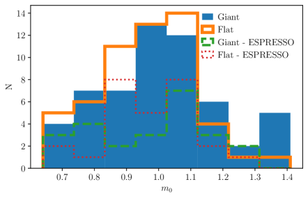
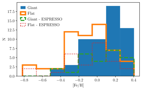
Figure 1: Masses (top panel) and metallicities (bottom panel) of the stars in our Giant and Flat samples (see Sect. 2).

We constructed our samples from two historical volume-limited giant-planet search surveys conducted with CORALIE (Udry et al. 2000) and HARPS (Lo Curto et al. 2010) spectrographs. These two historical surveys comprise a total of 2487 main-sequence G and K dwarfs, volume-limited to 57 pc, and were conducted at a typical precision of about 5 m/s for CORALIE and 2-3 m/s for HARPS over more than two decades.

We selected less active stars ($\log R^{\prime}_{HK}<-4.6$) and considered only stars closer than 52 pc. We defined two subsamples for our comparative study, composed of stars with similar mass distributions ranging from 0.65 to 1.4 $m_{\odot}$:

1. “Giant” sample (all 57 systems matching the criteria):

   • with at least one giant planet in their outer region ($m\sin i>100\penalty 10000\ m_{\oplus}$, $a>0.5$ AU),

   • no giant planet in their inner region ($a<0.5$ AU),

   • no highly eccentric orbits ($e<0.7$),

   • no high-mass companions ($m<30\penalty 10000\ m_{J}$ at 5 AU) based on Hipparcos-Gaia proper motion anomalies (PMA, see Kervella et al. 2022),

2. “Flat” sample (55 systems randomly selected among 73 systems matching the criteria):

   • at least 25 HARPS and 25 CORALIE pre-existing measurements spread over at least 8 years,

   • no signature of a giant planet from the analysis of available RVs,

   • no signature of a giant planet from the analysis of Hipparcos-Gaia PMA.

We obtained two successive ESO Large Programmes (LPs) on HARPS (108.22KV) and HARPS+ESPRESSO (112.25YG). In both campaigns, the aim was to explore the inner parts of these systems by taking advantage of preexisting measurements. We searched for ILPs in the super-Earth (SE; 3–10 $m_{\oplus}$) and Neptune-like (NE; 10–30 $m_{\oplus}$) ranges, with periods shorter than 50 d.

The goal of the first LP (108.22KV) was to obtain approximately 75 HARPS measurements for 26 systems belonging to the Giant sample. The second LP (112.25YG), which is on-going at the time of writing, aims to gather 50 HARPS measurements for all 112 systems and 25 ESPRESSO measurements for half of the sample (25 systems from the Giant sample and 27 from the Flat sample). Most systems already had HARPS measurements, with some having reached the 50, or even 75, measurement thresholds, allowing reliance on archival data where appropriate. We used exposure times of 15 minutes for HARPS and 12 minutes for ESPRESSO (split in sub-exposures for bright targets) to average out stellar oscillations (Dumusque et al. 2011).

We note that the two historical giant-planet search surveys were subject to the observer-excitement bias described above. Before our search for inner planets began, the stars in the Giant sample had a median of 109 CORALIE measurements, while the stars in the Flat sample had a median of 34 CORALIE measurements. However, the detection capacity for low-mass inner planets in our samples is dominated by the high-precision HARPS and ESPRESSO measurements, for which we ensured a homogeneous observing strategy. Moreover, these historical surveys are blind-search surveys (i.e., not transit follow-ups), so there is no bias toward stars with known inner companions. Thus, the observer-excitement bias in giant-planet search surveys could have increased the probability of detecting additional OGPs in systems that show a hint of OGP presence. However, the effect of this bias on the OGP-ILP correlation should be limited.

Fig. 1 shows the distribution of masses and metallicities of our two samples, as well as those of the sub-samples observed with ESPRESSO. These masses and metallicities were computed using the ARES+MOOG method (Sousa et al. 2021, see also Sect. 3). The mass distributions of the two samples are very similar (Fig. 1). Regarding metallicities, the Giant sample is biased toward higher metallicities than the Flat sample, due to the metallicity-planet correlation (Gonzalez 1998; Santos et al. 2001). However, both samples contain a large number of targets in the range $-0.4<[\mathrm{Fe/H}]<0.2$, allowing an unbiased comparison (with respect to metallicity) by excluding the most extreme targets in each sample. In the longer term, the Flat sample may be slightly refined for future observational programs to exclude the most metal-poor stars and include additional metal-rich stars that were randomly excluded.

Here, we present three inner planet detections from our analysis of the 26 systems observed during the first LP (108.22KV). Global statistical analysis of the sample will be performed in subsequent articles of this series.

3 Stellar properties

Table 1: Stellar parameters for HD 23079, HD 196067, and HD 86226.

Star	HD 23079	HD 196067	HD 86226
Spectral Type	F9.5V	G0V	G2V
$\pi$ (mas)	29.8633 $\pm$ 0.0194	25.0327 $\pm$ 0.0205	21.9301 $\pm$ 0.0267
$V$ (mag)	7.11	6.44	7.93
$B$ (mag)	7.68	7.05	8.563
$d$ (pc)	33.50${}^{+0.05}_{-0.02}$	40.0${}^{+0.05}_{-0.04}$	45.68${}^{+0.09}_{-0.08}$
$\rm T_{eff}\,(K)$	$5994^{+55}_{-64}$	$6072^{+83}_{-76}$	$6007^{+75}_{-71}$
$\rm[Fe/H]\,(dex)$	$-0.129\pm 0.041$	$0.213\pm 0.042$	$-0.015\pm 0.041$
$\log g\,$(cm s-2)	4.37 $\pm$ 0.02	4.09 $\pm 0.02$	4.41 $\pm 0.02$
$R_{*}(R_{\odot})$	1.08${}^{+0.02}_{-0.03}$	1.71${}^{+0.03}_{-0.04}$	1.03${}^{+0.02}_{-0.02}$
$M_{*}(M_{\odot})$	1.16${}^{+0.02}_{-0.03}$	1.16${}^{+0.13}_{-0.09}$	1.08${}^{+0.05}_{-0.05}$
$L_{*}(L_{\odot})$	1.35${}^{+0.08}_{-0.08}$	3.54${}^{+0.27}_{-0.20}$	1.24${}^{+0.09}_{-0.07}$
$\log R^{\prime}_{\rm HK}$	$-4.929\pm 0.014$	$-5.033\pm 0.022$	$-4.946\pm 0.012$
$P_{\mathrm{rot.}}$ (d)	$15.0\pm 2.6$	$22.5\pm 2.9$	$22.8\pm 3.0$
Age (Gyr)	$2.6\pm 1.2$	$4.2\pm 2.0$	$3.8\pm 1.8$

This section describes the fundamental parameters of HD 23079, HD 196067, and HD 86226, which are part of our Giant sample. Obtaining accurate stellar masses is crucial, as it directly impacts our estimates of the planetary (minimum) masses inferred from the RV time series. Values of effective temperature $T_{\text{eff}}$, stellar mass $M_{*}$, stellar luminosity $L_{*}$, stellar radius $R_{*}$, and distance $d$ were estimated using the ARIADNE (spectrAl eneRgy dIstribution bAyesian moDel averagiNg fittEr) Python package (Vines & Jenkins 2022).

The ARIADNE package fits the spectral energy distribution (SED) of a star using multiple stellar atmosphere model grids, including PHOENIX V2 (Husser et al. 2013), BT-Settl, BT-NextGen, BT-Cond (Allard et al. 2012), Castelli & Kurucz (Castelli & Kurucz 2003), and Kurucz (Kurucz 1993). The package automatically retrieves available broadband photometric data from various sources and performs an SED fit using the different models. The resulting fits are then compared using Bayesian model averaging, which yields estimates of the stellar parameters. All of the results presented here were obtained by running ARIADNE with default priors (see Table 2 of Vines & Jenkins 2022).

Because the SED does not precisely constrain the stellar metallicity [Fe/H] and surface gravity $\log g$, we derived these values using the ARES+MOOG method (Sneden 1973; Sousa et al. 2007, 2008; Sousa 2014; Sousa et al. 2015, 2021). Additionally, surface gravity values were obtained from the Gaia Early Data Release 3 (Gaia Collaboration et al. 2016; Riello et al. 2021) parallaxes and photometry. We computed the $\log R^{\prime}_{\rm HK}$ time series using Gomes da Silva et al. (2021); Rutten (1984) and derived estimates of the rotation period and age using Mamajek & Hillenbrand (2008). A summary of the derived stellar parameters is given in Table 1.

HD 23079

is an F9.5 V dwarf at a distance $d$ = 33.5 pc with a magnitude of $V$ = 7.11. The ARIADNE fit yields an effective temperature $T_{\text{eff}}$ = 5994 K and a mass estimate $M_{*}$ = 1.16 M_⊙. The star has a surface gravity $\log g$ = 4.37 cm s^-2 and a metallicity [Fe/H] = -0.129 dex.

HD 196067

is a G0 V star with magnitude $V$ = 6.44. From the ARIADNE analysis, we find that this star is located at a distance $d$ = 40 pc, has an effective temperature $T_{\text{eff}}$ = 6072 K, and a mass $M_{*}$ = 1.16 M_⊙. The surface gravity and metallicity are $\log g$ = 4.09 cm s^-2 and [Fe/H] = 0.213 dex, respectively.

HD 86226

is a G2 V dwarf with magnitude $V$ = 7.93 located at a distance $d$ = 45.68 pc. From the SED fit, we obtain an effective temperature $T_{\text{eff}}$ = 6007 K. This star has an estimated mass $M_{*}$ = 1.08 M_⊙, a metallicity [Fe/H] = -0.015 dex, and a surface gravity $\log g$ = 4.41 cm  s^-2.

4 Observations

This section describes the combined RV time series for the three targets from CORALIE and HARPS observations, with the addition of PFS observations for HD 86226.

The CORALIE instrument is an echelle spectrograph installed on the Euler Swiss telescope at La Silla Observatory in Chile since 1998. It underwent upgrades in 2007 and 2014, which led to possible RV offsets. We consider the three versions of CORALIE as different instruments: CORALIE98, CORALIE07, and CORALIE14. Accordingly, we adjusted for a different offset and a different jitter term for each CORALIE version. The HARPS instrument is also an echelle spectrograph at La Silla Observatory, installed on the 3.6m telescope since 2003. We distinguish two versions of HARPS as different instruments, HARPS03 and HARPS15, corresponding to before and after a fiber link upgrade performed in May 2015 (Lo Curto et al. 2015).

For HD 86226, we also used the PFS RV measurements from Teske et al. (2020). The PFS instrument is an echelle spectrograph installed on the 6.5m Magellan II telescope at Las Campanas Observatory in Chile. Its CCD was upgraded in 2018, and we distinguish two versions of the instrument, PFS1 and PFS2, corresponding to before and after this upgrade. We used these PFS RVs in addition to the CORALIE and HARPS time series.

A summary of the observations used in the analysis of the three targets is given in Table 2. The table lists both the number of spectra and the number of unique nights of observations for each instrument. In the following, we used nightly binned time series.

Table 2: Summary of observations used in our analysis.

		HD 23079		HD 196067		HD 86226
		#	avg. err.	#	avg. err.	#	avg. err.
CORALIE	spectra	129	3.89	116	4.02	116	4.41
	nights	123	3.88	112	3.83	114	4.34
HARPS	spectra	77	0.67	76	0.66	74	0.84
	nights	76	0.67	75	0.63	73	0.83
PFS	spectra	–	–	–	–	105	1.4
	nights	–	–	–	–	59	1.34

5 Analysis

We performed two analyses for the three systems: a simple periodogram analysis (Sect. 5.1) and posterior inference using a nested sampling approach (Sect. 5.2).

5.1 Periodogram analysis

As an initial, simple, and fast analysis, we performed a period search using the open-source kepmodel Python package (Delisle et al. 2016, 2020). We first defined a base model of the RV time series, with an offset and a jitter term for each instrument. The jitter term is added quadratically to the RV uncertainties. We performed a maximum-likelihood fit of the model, restricting the jitter terms to be lower than 20 $\mathrm{m}\,\mathrm{s}^{-1}$ (see Table 3). We then searched sequentially for planetary signals in the residuals of the RV time series by computing a periodogram and the associated false alarm probability (FAP; see Baluev 2008; Delisle et al. 2020). For low FAP values (below 0.1%), we selected the highest peak in the periodogram and computed an estimate of the planet’s orbital parameters (see Delisle et al. 2016; Delisle & Ségransan 2022). We then performed a global maximum likelihood fit, adjusting all planetary parameters as well as the instruments’ offsets and jitter terms. We iterated the procedure until no significant periodic signal was found in the residuals (i.e., $\mathrm{FAP}>0.1\%$).

5.2 Posterior sampling

To better determine the orbital architecture of the systems and estimate uncertainties on the orbital parameters, we explored the parameter space using a nested sampling approach. The same model was used for the three targets, but with different prior distributions for the outer companions. Since the detection of these outer companions is not in question, we set some priors based on the previous periodogram analysis. This choice does not significantly impact the resulting posterior distributions. For the inner part of the systems, we adopted weakly informative priors, since the goal was to detect lower-mass planets, if present.

The model then consists of the following components: a Keplerian function for the outer companion, up to two additional Keplerians for the inner part of the system, between-instrument RV offsets, a constant systemic velocity, and a Gaussian noise model per instrument that includes individual jitter terms. The prior distributions for the parameters are listed in Table 3.

We used the Gaia DR3 radial velocity measurement (Katz et al. 2023) to set the prior on the systemic velocity, $v_{\rm sys}$, and the associated uncertainty to assign a Gaussian prior for the between-instrument RV offsets. Even if relatively informative, these priors are much wider than the posteriors and do not influence the results. For the jitter terms, we assigned a modified log-uniform prior (see e.g. Gregory 2005) with a knee at 1 $\mathrm{m}\,\mathrm{s}^{-1}$ and an upper limit of 20 $\mathrm{m}\,\mathrm{s}^{-1}$. The number of additional Keplerians, $N_{p}$, was free in this analysis and was assigned a uniform prior from 0 to 2, motivated by the fact that the periodogram analysis from section 5.1 showed only one inner companion in each system. The orbital parameters of these two Keplerians share the same priors: a log-uniform distribution for the periods, between 1 day and the time span of the time series, a modified log-uniform distribution for the semi-amplitudes (with a knee at 1 $\mathrm{m}\,\mathrm{s}^{-1}$ and an upper limit of 100 $\mathrm{m}\,\mathrm{s}^{-1}$), a Kumaraswamy distribution (Kumaraswamy 1980) for the eccentricities, and uniform priors for the argument of periastron, $\omega$, and the mean anomaly, $M_{0}$. The Kumaraswamy distribution is very similar to the beta distribution proposed by Kipping (2013), but is easier to implement in nested sampling algorithms since its inverse cumulative distribution function has a closed form (see also Stevenson et al. 2025).

Table 3: Prior distributions used in the RV analysis.

Parameter	Units	Prior
general
$v_{\rm sys}$	$\mathrm{m}\,\mathrm{s}^{-1}$	$\mathcal{G}$ (RVGaia, $\sigma$RVGaia)
$v_{\rm offset,i}$	$\mathrm{m}\,\mathrm{s}^{-1}$	$\mathcal{G}$ (0, $\sigma$RVGaia)
$j$	$\mathrm{m}\,\mathrm{s}^{-1}$	$\mathcal{MLU}$ (1, 20)
outer companion
$P$	days	$\mathcal{LU}\left(0.8\!\cdot\!P_{\rm guess},1.2\!\cdot\!P_{\rm guess}\right)$
$K$	$\mathrm{m}\,\mathrm{s}^{-1}$	$\mathcal{U}\left(0.5\!\cdot\!K_{\rm guess},1.5\!\cdot\!K_{\rm guess}\right)$
$e$		$\mathcal{U}\left(0,1\right)$
$\omega$	rad	$\mathcal{U}\left(0,2\pi\right)$
$M_{0}$	rad	$\mathcal{U}\left(0,2\pi\right)$
additional Keplerians
$N_{p}$	days	$\mathcal{U}_{i}\left(0,2\right)$
$P$	days	$\mathcal{LU}\left(1,\Delta t\right)$
$K$	$\mathrm{m}\,\mathrm{s}^{-1}$	$\mathcal{MLU}\left(1,100\right)$
$e$		$\mathcal{K}\left(0.867,3.03\right)$
$\omega$	rad	$\mathcal{U}\left(0,2\pi\right)$
$M_{0}$	rad	$\mathcal{U}\left(0,2\pi\right)$

We sampled from the posterior distribution using kima (Faria et al. 2018), a package dedicated to the Bayesian analysis of RV time series. The code uses the diffusive nested sampling algorithm (Brewer et al. 2011) to explore the posterior and calculate the marginal likelihood, or evidence, of the model. The algorithm is a variant of classic nested sampling (Skilling 2006) with some unique advantages. It explores a mixture of nested distributions, each successively occupying smaller regions within the prior, guided by the likelihood function. It can handle distributions showing multimodality, strong parameter correlations, and phase transitions (see e.g. Buchner 2023), much like those typically encountered in the exoplanet detection problem (e.g. Ford 2005; Gregory 2005; Feroz et al. 2011). Moreover, the algorithm can handle so-called trans-dimensional models (Brewer 2014; Brewer & Donovan 2015), in which the number of parameters can change depending on an unknown number of components (Keplerian functions, in our case). We ran the algorithm for a fixed number of steps ($500\,000$), which guaranteed a sufficient effective sample size (ESS).

6 Results

HD 23079	HD 196067	HD 86226

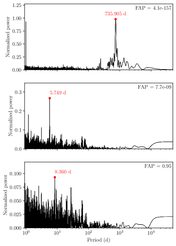
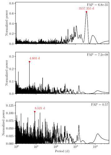
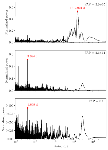
Figure 2: Periodograms of the raw RV time series (top panel) as well as of the residuals after subtracting the OGP (middle panel) and the ILP (bottom panel), for HD 23079 (left), HD 196067 (center), and HD 86226 (right).

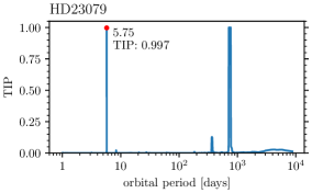
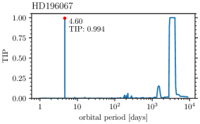
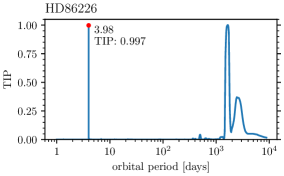
Figure 3: Posterior distributions for the orbital periods from the analysis of the three targets (left: HD 23079, center: HD 196067, right: HD 86226). The plots show the true inclusion probability (TIP), highlighting the peaks corresponding to the detected inner planets. Because the Keplerian signal of the outer planet is always included in the model, the TIP value for the outer planet period is, by definition, unity.

Table 4: Posteriors of the orbital parameters for HD 23079, HD 196067, and HD 86226.

Parameter	unit	HD 23079	HD 196067	HD 86226
$P_{\mathrm{b}}$	d	$735.7^{+0.4}_{-0.4}$	$3397^{+17}_{-14}$	$1616^{+46}_{-28}$
$U_{\mathrm{0,\,b}}$$=M_{\mathrm{0,\,b}}+\omega_{\mathrm{b}}$	deg	$107.0^{+0.9}_{-0.9}$	$-53.0^{+2.6}_{-2.2}$	$-66^{+16}_{-12}$
$K_{\mathrm{b}}$	$\mathrm{m}\,\mathrm{s}^{-1}$	$54.4^{+0.3}_{-0.4}$	$80^{+3}_{-4}$	$7.8^{+0.8}_{-0.6}$
$e_{\mathrm{b}}$		$0.072^{+0.012}_{-0.011}$	$0.561^{+0.011}_{-0.012}$	$0.07^{+0.09}_{-0.05}$
$\omega_{\mathrm{b}}$	deg	$29^{+15}_{-7}$	$142.0^{+1.5}_{-1.8}$	$37^{+100}_{-180}$
$m_{b}\sin i_{b}$	$M_{J}$	$2.66^{+0.05}_{-0.05}$	$5.42^{+0.20}_{-0.26}$	$0.49^{+0.05}_{-0.04}$
$P_{\mathrm{c}}$	d	$5.74894^{+0.00022}_{-0.00021}$	$4.60111^{+0.00024}_{-0.00024}$	$3.98450^{+0.00023}_{-0.00022}$
$U_{\mathrm{0,\,c}}$$=M_{\mathrm{0,\,c}}+\omega_{\mathrm{c}}$	deg	$156^{+10}_{-10}$	$-1^{+18}_{-17}$	$-10^{+24}_{-22}$
$K_{\mathrm{c}}$	$\mathrm{m}\,\mathrm{s}^{-1}$	$2.65^{+0.26}_{-0.27}$	$3.6^{+0.4}_{-0.4}$	$2.82^{+0.25}_{-0.26}$
$e_{\mathrm{c}}$		$0.07^{+0.09}_{-0.05}$	$0.12^{+0.12}_{-0.09}$	$0.05^{+0.07}_{-0.04}$
$\omega_{\mathrm{c}}$	deg	$247^{+64}_{-166}$	$278^{+41}_{-104}$	$170^{+108}_{-94}$
$m_{c}\sin i_{c}$	$M_{\oplus}$	$8.1^{+0.8}_{-0.8}$	$10.1^{+1.2}_{-1.2}$	$7.7^{+0.7}_{-0.7}$
Epoch	BJD	2 455 000	2 455 000	2 455 000

HD 23079

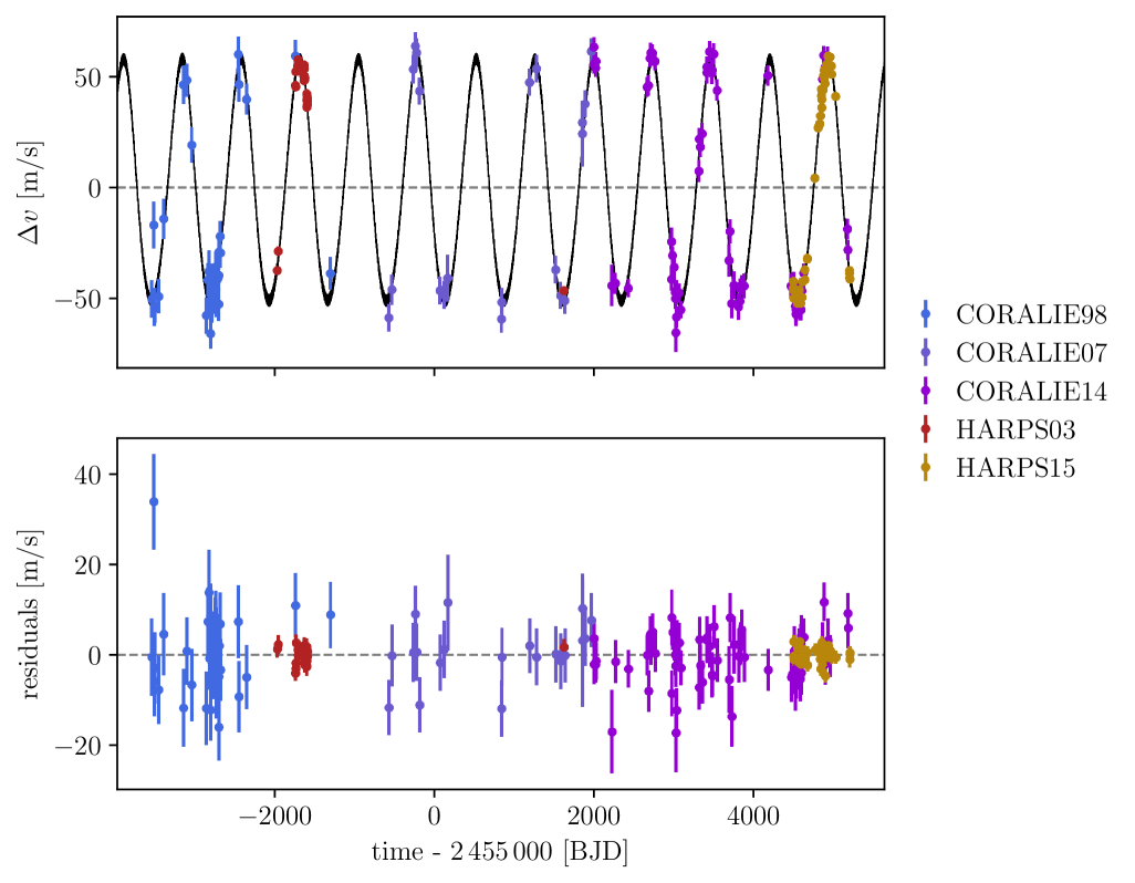
    HD 196067

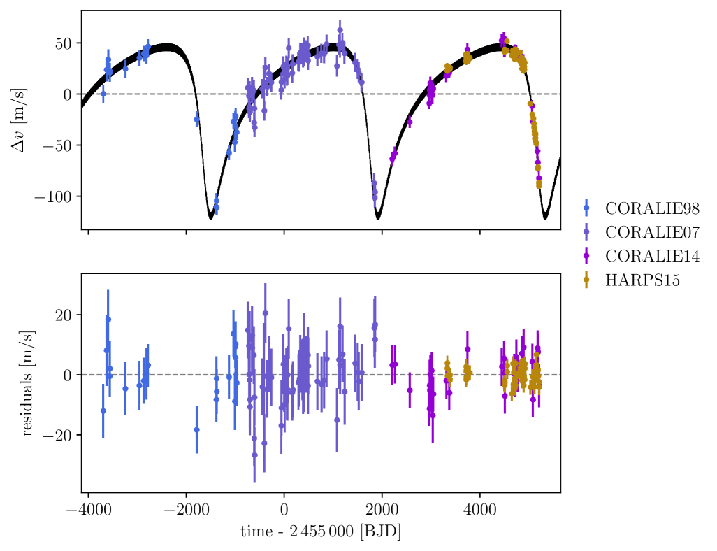
    HD 86226

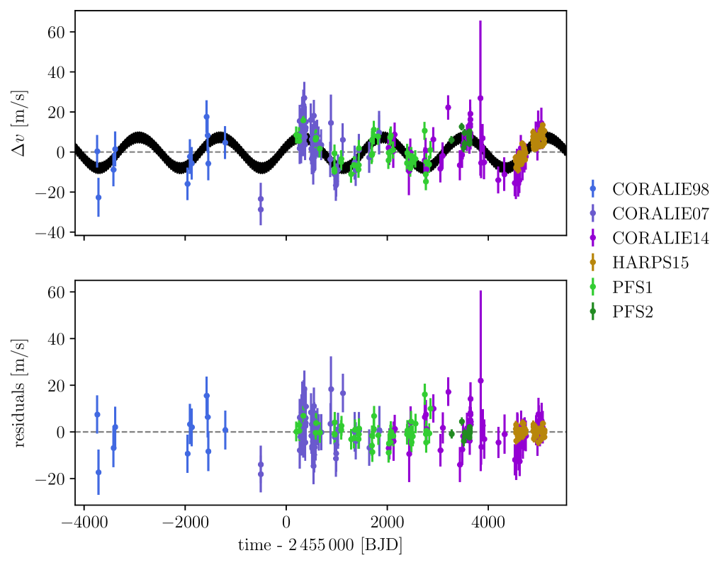
Figure 4: Time series (top panel) and residuals (bottom panel) of the maximum-likelihood fit for each target (HD 23079, HD 196067, and HD 86226).

HD 23079

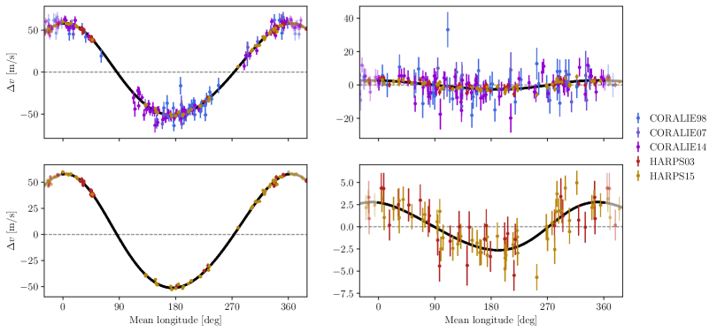
HD 196067

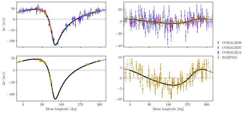
HD 86226

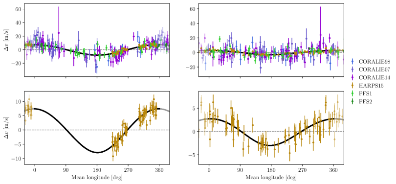
Figure 5: Top panel: Residuals of the maximum-likelihood fit phase-folded at the periods of the two detected planets, showing the outer giant (left) and lower-mass inner planet (right) for each target (HD 23079, HD 196067, and HD 86226). Bottom panel: Same residuals, but showing only the HARPS data.

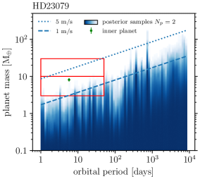
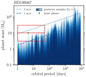
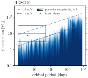
Figure 6: Compatibility limits from the analysis of the three targets (left: HD 23079, center: HD 196067, right: HD 86226). The plots show a color map of the posterior density for planet mass in orbital period bins, for all samples with $N_{p}=2$ (i.e., with a total of three Keplerians, including the OGP). Green points indicate detected inner planets with corresponding mass uncertainties. Dashed and dotted blue lines indicate masses corresponding to 1 and 5 m/s semi-amplitude Keplerians, respectively. Masses are calculated using the stellar masses from Table 1. Red boxes highlight the SE (3–10 $m_{\oplus}$) and NE (10–30 $m_{\oplus}$) mass ranges within 50 d.

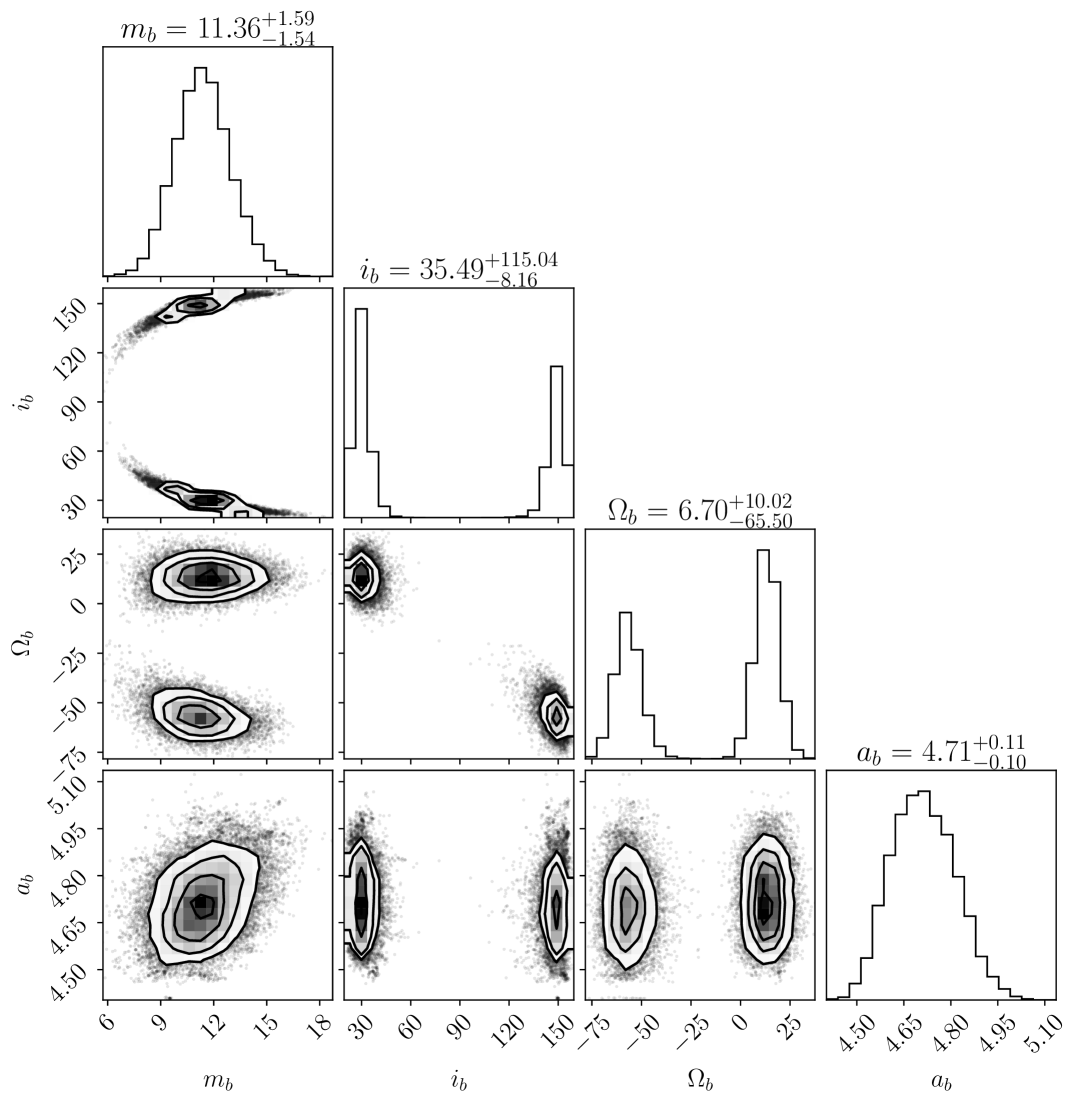
Figure 7: Posterior distributions from the orvara fit of HD 196067 (see Sect. 6).

Fig. 2 shows successive periodograms of the raw RV time series and after subtracting planetary signal for the three targets (HD 23079, HD 196067, and HD 86226). In all three systems, the periodogram analysis clearly indicates the detection of two planets, an OGP and an ILP. These detections are significant, as the FAP of all six planet signals are lower than $10^{-7}$. The FAP of the residuals after subtracting the planetary signals are above 10% in all three time series, indicating that no clear signal remains unmodeled in the residuals.

We show the true inclusion probability (TIP) periodograms based on the kima posterior sampling in Fig. 3. The TIP (see Hara et al. 2022) is the posterior probability (conditioned on the data) of having at least one planet in a small period interval around a given period $P$, or equivalently, in a small frequency interval $\left[f-\Delta f/2,f+\Delta f/2\right]$ around a frequency $f=1/P$. The TIP has been mathematically shown to be an optimal exoplanet detection criterion, in the sense that it maximizes the expected number of true detections for a given tolerance to false detections (see Hara et al. 2024). The TIP periodograms of Fig. 3 were obtained using $\Delta f=1/T_{\mathrm{span}}$ (where $T_{\mathrm{span}}$ is the time span of the observations) and by scanning the frequency $f$ over a finer grid ($\Delta f/10$) to ensure that local maxima of the TIP were not missed. The TIP is marginalized over the number of planets included in the model. In the kima runs, we always included the OGP in the model and allowed the number of additional planets to vary between zero and two (thus the total number of planets is free between one and three). Therefore, by construction, the TIP is one at the OGP’s period because we enforced the presence of this already known planet in the model. For the ILP, the TIP values exceed 99% for all three targets (see Fig. 3), which confirms the detection of these planets. As in the classical periodograms, we do not find any additional significant peak in the TIP periodograms.

The parameters of the maximum-likelihood solution and of the posterior sampling are given in Table 5 for all three systems. Table 4 provides a shorter version of this table that contains only the posteriors of the orbital parameters. The two estimates are in good agreement for all parameters. As final estimates, we quote the maximum-likelihood values and the 68% credible intervals from the posteriors. The RV time series and the residuals from the maximum-likelihood solution are shown in Fig. 4 and are phase-folded in Fig. 5. Our solution for HD 86226 agrees with Teske et al. (2020), with a slight refinement to the mass estimate for the inner planet (c).

From the kima analysis, we also derived so-called compatibility limits, corresponding to the orbital periods and masses of undetected planets that remain compatible with the available data (see, e.g., Standing et al. 2022 and Figueira et al. 2025). In practice, these limits were obtained from all posterior samples with $N_{p}=2$ (thus with a total of three Keplerians in the model, accounting for the OGP) and are therefore available from a single run of the algorithm. These limits do not rely on injection and recovery of signals (sinusoidal or otherwise), do not require the subtraction of a best-fit solution, and marginalize over other orbital parameters, such as eccentricity. The compatibility limits for the three targets are shown in Fig. 6. The adjusted HARPS jitter is larger for HD 196067 than for the other two targets (see Table 5), due to a larger scatter in the residuals for this star. This results in slightly worse detection limits for this source (see Fig. 6). For HD 86226, the compatibility limits shown in Fig. 6 include PFS RVs in addition to CORALIE and HARPS data. However, excluding PFS data does not significantly change the detection limits for orbital periods shorter than a year (see Appendix B).

All three targets were observed by TESS. We checked whether the inner planets detected for each star transit in the available TESS data. This analysis is presented in Appendix C. We conclude that HD 23079 and HD 196067 are not transiting, while the known transit of HD 86226 is clearly recovered (see Teske et al. 2020).

To constrain the inclinations of the OGP and thereby their true masses, we jointly fit RV and astrometric data from the Hipparcos-Gaia Catalog of Accelerations (HGCA; Brandt 2021) using orvara (Brandt et al. 2021). The HGCA provides the $\chi^{2}$ value for each star, which should follow a $\chi^{2}$ distribution with 2 degrees of freedom if the star lacks acceleration. The $\chi^{2}$ is 0.709 (p-value of $70\%$) for HD 23079, 64.9 (p-value of $8\times 10^{-15}$) for HD 196067, and 1.12 (p-value of $57\%$) for HD 86226. Thus, we detect a highly significant acceleration for HD 196067, and nonsignificant accelerations for HD 23079 and HD 86226. We used a customized version of orvara, which accommodates a larger set of priors, in particular for between-instrument RV offsets. All priors were set as in Sect. 5.2, except for RV jitters (log-uniform distribution from 0.1 $\mathrm{m}\,\mathrm{s}^{-1}$ to 20 $\mathrm{m}\,\mathrm{s}^{-1}$), and for the semi-major axis (log-uniform from 0.0025 AU to 500 AU) and mass (log-uniform from $10^{-7}M_{\odot}$ to 1 $M_{\odot}$) of the planets, which were explored instead of the period and RV semi-amplitude. We included a Gaussian prior on the period of the ILP (the maximum likelihood solution from Table 5), to facilitate the convergence of the fit. We excluded the binary companion to HD 196067, HD 196068, from the orvara fit, because it lies at a separation of $>16$ arcseconds ($\approx 800$ AU, Gaia Collaboration et al. 2023), too far to be detected in our RVs or in HGCA astrometry of HD 196067.

We ran orvara with ten temperatures, each with 150 walkers, for 150,000 steps. As expected, we are unable to constrain the inclination of the three ILPs. We also find no inclination constraints for the OGP of HD 23079 and HD 86226, which is also expected given the nonsignificant Hipparcos-Gaia accelerations for these two stars.

The posteriors of the orvara orbital fit for HD 196067 are shown in Fig. 7. We find that the true mass of the OGP of HD 196067 is $m_{b}=11.4\pm 1.6\penalty 10000\ M_{J}$. The inclination distribution is bimodal, with two almost symmetric modes at $i=29.7^{+5.0}_{-3.8}$ deg and $i=149.2^{+3.9}_{-5.1}$ deg. The mode at 29.7 deg appears slightly favored by the data. We find a semi-major axis of $4.71^{+0.11}_{-0.10}$ AU. These results update those presented in Li et al. (2021), providing finer constraints on the orbital parameters of the OGP (a factor of two on the semi-major axis) thanks to our additional RV data.

7 Discussion

This article presents the three inner planet detections obtained by monitoring a sample of 26 stars with known outer giant planets using HARPS. A dedicated statistical study including these 26 stars and additional well-monitored stars with and without outer giant planets will be presented in a subsequent paper. We note here that two of these inner planets lie in the SE range (3–10 $m_{\oplus}$), and one is in the NE range (10–30 $m_{\oplus}$), slightly above the SE-NE limit.

The estimated occurrences of SE and NE below 50 d in the general population are $0.11\pm 0.03$ and $0.08\pm 0.02$, respectively (Bashi et al. 2020). If the occurrence rates of SE and NE were the same in our sample as in the general population (i.e., without impact from the giant planets), we would typically expect to detect 2.9 SE and 2.1 NE (about five inner planets in total). From the compatibility limits of the three targets presented here (see Fig. 6), we see that our observing strategy enables the detection of NE below 50 d with very high completeness. For SE, completeness is very poor above 10 d, and we aim to improve this in the long term with additional HARPS and ESPRESSO measurements (on-going ESO LP). Since we used the same observing strategy for the 26 targets in our sample, we can extrapolate, as a first approximation, that similar detection limits are reached for the 23 other targets, for which we do not find any ILP.

We detect fewer inner planets than expected from the general population occurrence rates, but given the small-number statistics and without a proper statistical analysis correcting for completeness, we cannot conclude on a slight enhancement or inhibition of ILP in the presence of OGP. However, these results are difficult to reconcile with the claim of Zhu & Wu (2018); Bryan et al. (2019) that $p(\mathrm{SE}\cup\mathrm{NE}|\mathrm{{\rm OGP}})$ is close to 90%.

Interestingly, the three ILPs detected in this study all have periods below 6 d. While this could be due to small-number statistics and reduced detection efficiency at longer periods (see Fig. 6), these three detections are significant, and we should have been able to detect, albeit with lower confidence, similar-mass planets up to 20 d . This observation, if confirmed with a rigorous statistical analysis, would be in agreement with the findings of Van Zandt et al. (2025) that ILPs tend to be found at shorter periods in systems with an OGP than in the general population.

Data availability

The RV data for the three targets discussed in this work, as well as kima posterior samples, are available on the DACE platform: https://doi.org/10.82180/dace-inner001.

Appendix A Extended posteriors table

Table 5: Maximum likelihood solution and kima posteriors for HD 23079, HD 196067, HD 86226.

		HD 23079		HD 196067		HD 86226
Parameter	unit	max-likelihood	kima posterior	max-likelihood	kima posterior	max-likelihood	kima posterior
$v_{\mathrm{sys.}}$	$\mathrm{m}\,\mathrm{s}^{-1}$	$573.801{\,\scriptstyle\pm 0.319}$	$574.0\pm 0.5$	$-10945.854{\,\scriptstyle\pm 0.922}$	$-10945.0^{+1.5}_{-1.6}$	$19776.047{\,\scriptstyle\pm 0.825}$	$19776.5^{+1.6}_{-1.5}$
$v_{\mathrm{CORALIE98}}$	$\mathrm{m}\,\mathrm{s}^{-1}$	$65.81{\,\scriptstyle\pm 1.30}$	$65.9\pm 1.4$	$64.74{\,\scriptstyle\pm 2.26}$	$65.5^{+3.0}_{-2.8}$	$-31.82{\,\scriptstyle\pm 3.01}$	$-33^{+4}_{-5}$
$v_{\mathrm{CORALIE07}}$	$\mathrm{m}\,\mathrm{s}^{-1}$	$70.44{\,\scriptstyle\pm 1.48}$	$70.6\pm 1.5$	$61.83{\,\scriptstyle\pm 1.35}$	$62.1^{+1.6}_{-1.5}$	$-36.89{\,\scriptstyle\pm 1.31}$	$-37.6^{+1.7}_{-2.9}$
$v_{\mathrm{CORALIE14}}$	$\mathrm{m}\,\mathrm{s}^{-1}$	$95.196{\,\scriptstyle\pm 0.634}$	$95.2^{+0.7}_{-0.6}$	$88.36{\,\scriptstyle\pm 1.25}$	$88.7^{+1.5}_{-1.4}$	$-17.26{\,\scriptstyle\pm 1.05}$	$-17.6^{+1.3}_{-1.5}$
$v_{\mathrm{HARPS03}}$	$\mathrm{m}\,\mathrm{s}^{-1}$	$-12.112{\,\scriptstyle\pm 0.525}$	$-11.9\pm 0.7$	–	–	–	–
$v_{\mathrm{PFS1}}$	$\mathrm{m}\,\mathrm{s}^{-1}$	–	–	–	–	$-160.29{\,\scriptstyle\pm 1.08}$	$-160.7^{+1.7}_{-2.2}$
$v_{\mathrm{PFS2}}$	$\mathrm{m}\,\mathrm{s}^{-1}$	–	–	–	–	$-162.46{\,\scriptstyle\pm 0.832}$	$-163.3^{+1.6}_{-2.1}$
$\sigma_{\mathrm{CORALIE98}}$	$\mathrm{m}\,\mathrm{s}^{-1}$	$6.46{\,\scriptstyle\pm 1.10}$	$6.8^{+1.4}_{-1.2}$	$6.44{\,\scriptstyle\pm 1.85}$	$9.2^{+2.6}_{-2.9}$	$7.32{\,\scriptstyle\pm 2.20}$	$8.3^{+3.1}_{-2.4}$
$\sigma_{\mathrm{CORALIE07}}$	$\mathrm{m}\,\mathrm{s}^{-1}$	$5.28{\,\scriptstyle\pm 1.21}$	$5.4^{+1.6}_{-1.3}$	$8.91{\,\scriptstyle\pm 1.01}$	$8.7^{+1.1}_{-1.0}$	$7.067{\,\scriptstyle\pm 0.914}$	$7.1^{+1.1}_{-0.9}$
$\sigma_{\mathrm{CORALIE14}}$	$\mathrm{m}\,\mathrm{s}^{-1}$	$3.019{\,\scriptstyle\pm 0.651}$	$3.0^{+0.7}_{-0.8}$	$4.86{\,\scriptstyle\pm 1.02}$	$4.8^{+1.3}_{-1.1}$	$5.287{\,\scriptstyle\pm 0.826}$	$5.1^{+1.0}_{-0.9}$
$\sigma_{\mathrm{HARPS03}}$	$\mathrm{m}\,\mathrm{s}^{-1}$	$1.684{\,\scriptstyle\pm 0.266}$	$1.9^{+0.4}_{-0.3}$	–	–	–	–
$\sigma_{\mathrm{HARPS15}}$	$\mathrm{m}\,\mathrm{s}^{-1}$	$1.253{\,\scriptstyle\pm 0.174}$	$1.46^{+0.27}_{-0.26}$	$2.381{\,\scriptstyle\pm 0.215}$	$2.48^{+0.33}_{-0.25}$	$1.435{\,\scriptstyle\pm 0.163}$	$1.54^{+0.21}_{-0.18}$
$\sigma_{\mathrm{PFS1}}$	$\mathrm{m}\,\mathrm{s}^{-1}$	–	–	–	–	$4.044{\,\scriptstyle\pm 0.522}$	$4.1^{+0.7}_{-0.5}$
$\sigma_{\mathrm{PFS2}}$	$\mathrm{m}\,\mathrm{s}^{-1}$	–	–	–	–	$1.590{\,\scriptstyle\pm 0.408}$	$1.8^{+0.6}_{-0.4}$
$P_{\mathrm{b}}$	d	$735.740{\,\scriptstyle\pm 0.220}$	$735.7^{+0.4}_{-0.4}$	$3413.7{\,\scriptstyle\pm 10.5}$	$3397^{+17}_{-14}$	$1609.5{\,\scriptstyle\pm 19.4}$	$1616^{+46}_{-28}$
$U_{\mathrm{0,\,b}}$$=M_{\mathrm{0,\,b}}+\omega_{\mathrm{b}}$	deg	$107.069{\,\scriptstyle\pm 0.563}$	$107.0\pm 0.9$	$-50.31{\,\scriptstyle\pm 1.45}$	$-53.0^{+2.6}_{-2.2}$	$-70.55{\,\scriptstyle\pm 8.07}$	$-66^{+16}_{-12}$
$K_{\mathrm{b}}$	$\mathrm{m}\,\mathrm{s}^{-1}$	$54.386{\,\scriptstyle\pm 0.248}$	$54.4^{+0.3}_{-0.4}$	$82.57{\,\scriptstyle\pm 1.91}$	$80^{+3}_{-4}$	$7.653{\,\scriptstyle\pm 0.539}$	$7.8^{+0.8}_{-0.6}$
$e_{\mathrm{b}}$		$0.07348{\,\scriptstyle\pm 0.00651}$	$0.072^{+0.012}_{-0.011}$	$0.56292{\,\scriptstyle\pm 0.00703}$	$0.561^{+0.011}_{-0.012}$	$0.0389{\,\scriptstyle\pm 0.0677}$	$0.07^{+0.09}_{-0.05}$
$\omega_{\mathrm{b}}$	deg	$33.20{\,\scriptstyle\pm 4.92}$	$29^{+15}_{-7}$	$142.835{\,\scriptstyle\pm 0.966}$	$142.0^{+1.5}_{-1.8}$	$201.4{\,\scriptstyle\pm 70.4}$	$37^{+100}_{-180}$
$m_{b}\sin i_{b}$	$M_{J}$	$2.66{\,\scriptstyle\pm 0.05}$	$2.66\pm 0.05$	$5.58{\,\scriptstyle\pm 0.44}$	$5.42^{+0.20}_{-0.26}$	$0.46{\,\scriptstyle\pm 0.04}$	$0.49^{+0.05}_{-0.04}$
$P_{\mathrm{c}}$	d	$5.748913{\,\scriptstyle\pm 0.000204}$	$5.74894^{+0.00022}_{-0.00021}$	$4.601088{\,\scriptstyle\pm 0.000192}$	$4.60111\pm 0.00024$	$3.984436{\,\scriptstyle\pm 0.000217}$	$3.98450^{+0.00023}_{-0.00022}$
$U_{\mathrm{0,\,c}}$$=M_{\mathrm{0,\,c}}+\omega_{\mathrm{c}}$	deg	$155.61{\,\scriptstyle\pm 9.54}$	$156\pm 10$	$-3.3{\,\scriptstyle\pm 14.4}$	$-1^{+18}_{-17}$	$-17.0{\,\scriptstyle\pm 22.3}$	$-10^{+24}_{-22}$
$K_{\mathrm{c}}$	$\mathrm{m}\,\mathrm{s}^{-1}$	$2.702{\,\scriptstyle\pm 0.252}$	$2.65^{+0.26}_{-0.27}$	$3.762{\,\scriptstyle\pm 0.396}$	$3.6\pm 0.4$	$2.866{\,\scriptstyle\pm 0.253}$	$2.82^{+0.25}_{-0.26}$
$e_{\mathrm{c}}$		$0.097{\,\scriptstyle\pm 0.124}$	$0.07^{+0.09}_{-0.05}$	$0.235{\,\scriptstyle\pm 0.118}$	$0.12^{+0.12}_{-0.09}$	$0.0619{\,\scriptstyle\pm 0.0817}$	$0.05^{+0.07}_{-0.04}$
$\omega_{\mathrm{c}}$	deg	$283.4{\,\scriptstyle\pm 47.2}$	$247^{+64}_{-166}$	$295.5{\,\scriptstyle\pm 23.8}$	$278^{+41}_{-104}$	$144.6{\,\scriptstyle\pm 91.4}$	$170^{+108}_{-94}$
$m_{c}\sin i_{c}$	$M_{\oplus}$	$8.26{\,\scriptstyle\pm 0.79}$	$8.1\pm 0.8$	$10.4{\,\scriptstyle\pm 1.39}$	$10.1\pm 1.2$	$7.45{\,\scriptstyle\pm 0.7}$	$7.7\pm 0.7$
reference epoch		2 455 000 BJD		2 455 000 BJD		2 455 000 BJD
$N$		199		187		246
$\log L_{\rm max}$		-537.8944		-569.7350		-690.3457
$\log Z$		-625.97		-644.7		-767.46
$\mathcal{I}$		77.19		67.56		70.37

Appendix B Compatibility limits without PFS data

The compatibility limits shown in Fig. 6 (right) for HD 86226 include PFS radial velocities in addition to CORALIE and HARPS data. This is useful to assess whether additional planets could still hide in this system. However, in order to assess the sensitivity of our observing programme to detect small planets, we additionally produced a compatibility map using only CORALIE and HARPS data, which is the typical case for most targets in our programme.

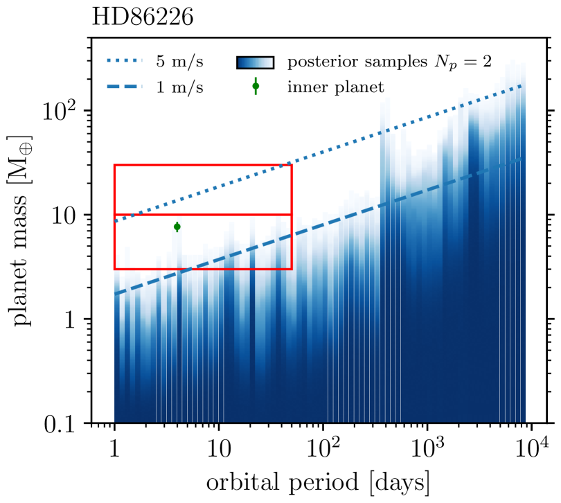
Figure 8: Compatibility limits of HD 86226 including (top, see also Fig. 6) or not (bottom) PFS RVs in the analysis.

Both compatibility maps are shown in Fig. 8 for comparison. Adding the PFS data improves the long-period planets detectability but only marginally the short periods planets detectability. Short periods are well covered by HARPS measurements which have a significantly better precision than PFS measurements (see Table 2). Thus the addition of PFS data does not improve much the SNR at short period. For longer periods, including PFS measurements allows to have a longer baseline covered with high-precision RV instruments.

Appendix C Inner planets transit-search with TESS

In this appendix we present the search for potential transits of the inner planets detected for each star. For this analysis, we fix the stellar parameters at their median value reported in Table 1. For each star, the raw PDCSAP flux was downloaded using the lightkurve package. We obtained sectors 3, 4, 30 and 31 for HD 23079, sectors 13, 27, 66 and 67 for HD 196067, and sectors 9, 35 and 62 for HD 86226. Then, we split the time series into half-sectors in order to model the noise on each independently. We detrend the data with a B-spline using the linmarg Python package (see Leleu et al. 2023). The spacing of the nodes of the B-spline is chosen to be 3 times the transit duration of a planet on a circular orbit at the period of the RV detection and with a null impact parameter.

We first performed a BLS search around the period found in RV with a 3$\sigma_{P_{c}}$ window in period ($\sigma$ is chosen as the max of the two errors reported in Table 5) around the median $\bar{P_{c}}$, to see if there is an obvious transit in the data. We found HD 86226 c with properties similar to the one reported in Teske et al. (2020), but no signal with SNR more than 4 in this pre-detrended dataset for HD 23079 c and HD 196067 c.

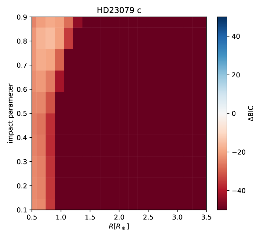
Figure 9: Model comparison map for HD 23079 c, for radius ranging from 0.5 to 3.5 $R_{\oplus}$ and impact parameters ranging from 0.1 to 0.9. The colors indicate the value of the $\Delta BIC$, red indicating that the null model is favoured, while blue indicates that the planet model is favoured. a value of $|\Delta BIC|>20$ is usually considered to be a compelling evidence for the model.

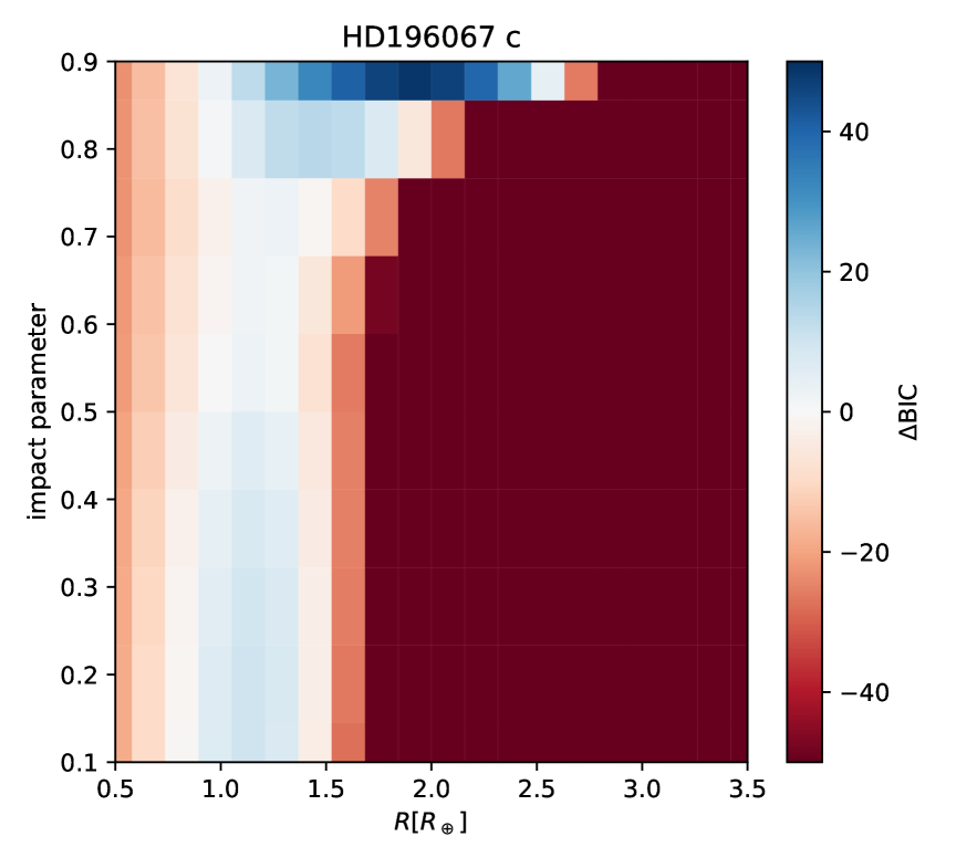
Figure 10: Model comparison map for HD 196067 c, see Fig. 9 the text for more detail.

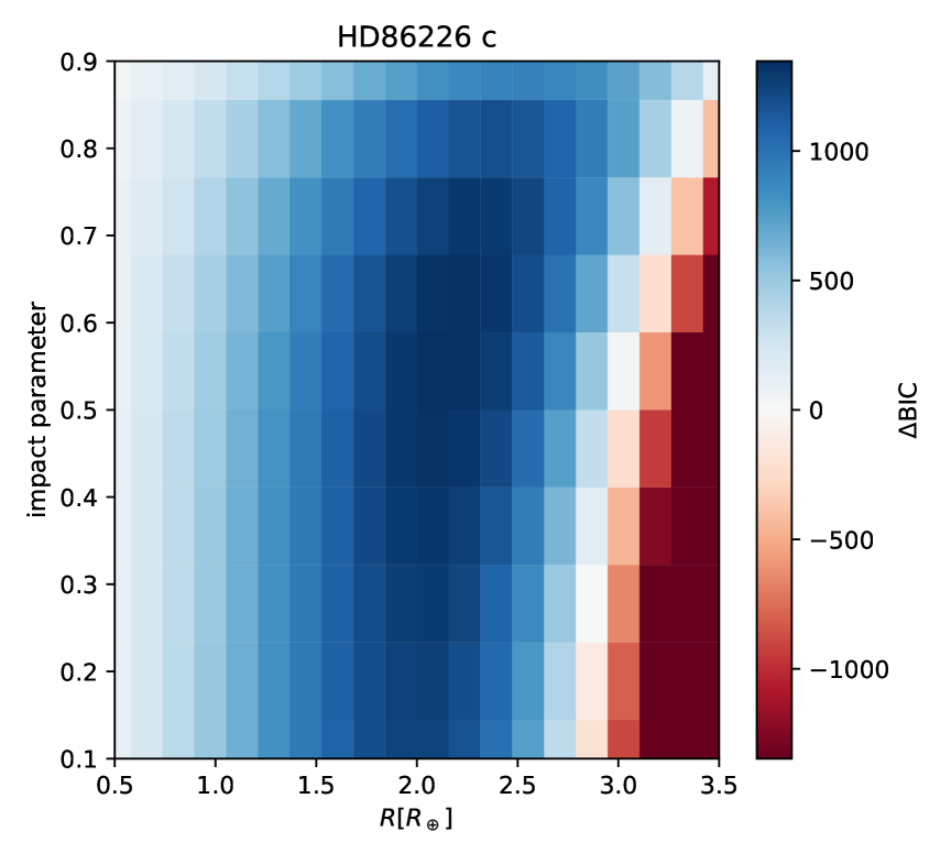
Figure 11: Model comparison map for HD 86226 c, see Fig. 9 the text for more detail.

We then computed a model comparison map for each planet with a simultaneous noise and planet modelling. To do so, we first identify potentially problematic parts of the light curves using the pre-detrended data. We start by flagging the data points that are at a larger separation from the mean value than 4 times the standard deviation. We then binned the data with a 30 min cadence. We then checked, for each half-sector, if the standard deviation of the flux was 2.5 larger than the minimum standard deviation of all the binned half-sector for that star. This notably lead to the removal of sector 66 for HD 196067 which had a much larger scatter than the others. All other half-sectors were kept. We then identified all time stamps that were removed in the detrended light curves, and removed it from the raw data. Restarting from the masked raw data, we then estimated the likelihood of the null model $\mathcal{L}_{0}$, only applying the detrending. Then, for a grid of planetary radii $R_{c}$ and impact parameters $b_{c}$, we explored a grid of orbits ranging the $3\sigma$ interval both in period and $\lambda_{0}$ for each inner planet. The step in $\lambda_{0}$ is set such that the time of transit around the reference epoch varies by 10 min steps. The step in period is set such as the last transit varies by steps of 15 min ($\delta P=6\sigma_{P_{c}}(t_{max}-t_{min})/\bar{P_{c}})/96$. Then, for each couple ($R_{c}$, $b_{c}$), we save the highest likelihood $\mathcal{L}_{p}$ in the grid ($t_{0,c}$, $P_{c}$), with a simultaneous modelling of the transits of the planet and the noise model (the aforementioned B-splines). We then compute the $\Delta BIC=2(\mathcal{L}_{p}-\mathcal{L}_{0})-4\log(N_{bins})$.

Figures 9, 10 and 11 show the model comparison maps for HD 23079 c, HD 196067 c and HD 86226 c, respectively. For HD 23079 c and HD 86226 c, the interpretation of the maps are straightforward: existing data exclude a planetary transit for HD 23079 c, while the known $\sim 2R_{\oplus}$ planet is favoured for HD 86226 c (Teske et al. 2020). For HD 196067 c, we notice a $\Delta BIC\sim 48$ for $R_{c}\sim 1.9R_{\oplus}$ and an impact parameter of 0.9. We investigated this solution by estimating $\Delta BIC$ per half-sector instead of the whole dataset. It turns out that $\Delta BIC$ is only positive for the first half of sector 13, and negative for the 5 other half-sectors. Upon visual inspection of the lightcurve, a single dip of the flux over a timescale of $\sim 1h$ seems to be responsible for the positive value of the $\Delta BIC$ in the first half of sector 13. We therefore conclude that the planet is not transiting.