Tracer diffusion coefficients in a sheared granular gas. Exact results

Abstract

The diffusion of tracer particles immersed in a granular gas under uniform shear flow (USF) is analyzed within the framework of the inelastic Boltzmann equation. Two different but complementary approaches are followed to achieve exact results. First, we maintain the structure of the Boltzmann collision operator but consider inelastic Maxwell models (IMM). Using IMM allows us to compute the collisional moments of the Boltzmann operator without knowing the velocity distribution functions of the granular binary mixture explicitly. Second, we consider a kinetic model of the Boltzmann equation for inelastic hard spheres (IHS). This kinetic model is based on the equivalence between a gas of elastic hard spheres subjected to a drag force proportional to the particle velocity and a gas of IHS. We solve the Boltzmann–Lorentz kinetic equation for tracer particles using a generalized Chapman–Enskog–like expansion around the shear flow distribution. This reference distribution retains all hydrodynamic orders in the shear rate. The mass flux is obtained to first order in the deviations of the concentration, pressure, and temperature from their values in the reference state. Due to the velocity space anisotropy induced by the shear flow, the mass flux is expressed in terms of tensorial quantities rather than the conventional scalar diffusion coefficients. The exact results derived here are compared with those previously obtained for IHS by using different approximations [JSTAT P02012 (2007)]. The comparison generally shows reasonable quantitative agreement, especially for IMM results. Finally, we study segregation by thermal diffusion as an application of the theory. The phase diagrams illustrating segregation are shown and compared with IHS results, demonstrating qualitative agreement.

I Introduction

When granular media are externally excited they behave like a fluid. In these conditions (rapid flow conditions), the tools of the classical kinetic theory of gases (conveniently adapted to dissipative dynamics) can be used to derive the corresponding hydrodynamic equations with explicit expressions for the transport coefficients Campbell (1990); Goldhirsch (2003); Brilliantov and Pöschel (2004); Rao and Nott (2008); Garzó (2019). A granular gas is typically modeled as a gas of hard spheres with inelastic collisions. In the simplest version, the spheres are assumed to be completely smooth, and inelasticity in collisions is accounted for only through a constant positive coefficient of normal restitution. In the dilute regime, the inelastic version of the Boltzmann equation Brilliantov and Pöschel (2004); Garzó (2019) has been solved by means of the Chapman–Enskog method Chapman and Cowling (1970) and the set of coupled linear integral equation verifying the Navier–Stokes transport coefficients has been also derived. As with elastic collisions Chapman and Cowling (1970); Ferziger and Kaper (1972), for hard spheres usually these integral equations are approximately solved by considering the first few terms in a Sonine polynomial expansion of the distribution function. This procedure can be extended to the more realistic case of granular mixtures, namely when grains have different masses and/or diameters. However, the problem is more complex than that of a monocomponent gas since the number of transport coefficients is greater and they depend on more parameters (see, for example, Refs. Jenkins and Mancini (1987, 1989); Zamankhan (1995); Garzó and Dufty (2002); Garzó et al. (2006); Serero et al. (2006); Garzó and Montanero (2007); Garzó et al. (2007a, b)). Additionally, determining the transport properties from the Boltzmann equation for both elastic and/or inelastic hard spheres is a very difficult task for far from equilibrium states (i.e., beyond the Navier–Stokes domain).

Due to the aforementioned difficulties, alternative approaches are commonly used in kinetic theory to obtain exact results. One possibility is to maintain the intricate mathematical structure of the Boltzmann collision operator while assuming a different interaction model: the so-called inelastic Maxwell model (IMM). To the best of our knowledge, this interaction model was introduced independently in Refs. Ben-Naim and Krapivsky (2000) and Bobylev et al. (2000) at the beginning of the 21st century. The main reason for introducing IMM was to analyze in a clean way the overpopulation associated with the high energy tails of the distribution function in the homogeneous cooling state (HCS) Bobylev et al. (2000); Ernst and Brito (2002a, b); Baldassarri et al. (2002); Krapivsky and Ben-Naim (2002a, b); Ernst and Brito (2002c); Bobylev and Cercignani (2002); Ben-Naim and Krapivsky (2003); Bobylev and Cercignani (2003); Bobylev et al. (2003); Ernst et al. (2006); Barrat et al. (2007).

As with the conventional Maxwell molecules Ernst (1981) (which are defined by a repulsive potential inversely proportional to the fourth power of the distance for a three-dimensional gas), the collision rate for IMM is independent of the relative velocity of the colliding spheres. This contrasts with the inelastic hard sphere (IHS) model, in which the collision rate is proportional to the relative velocity. The main advantage of using IMM instead of IHS is that a collisional moment of degree $k$ can be expressed in terms of velocity moments of degree $k$ or smaller than $k$, without knowing the velocity distribution function. This property allows one to obtain the exact forms of the Navier-Stokes transport coefficients, as well as the rheological properties of sheared granular gases Garzó (2019). However, since IMM’s scattering rules are the same as IHS’, these models do not describe real particles because they do not interact according to a given potential law. In any case, many researchers working in the field recognize that the cost of sacrificing physical realism can be offset by the number of exact analytical results obtained using IMM. Apart from this aspect, it should be noted that some experiments involving magnetic grains with dipolar interactions have been well described by IMM Kohlstedt et al. (2005).

Another possible approach to achieving exact results is considering simpler kinetic models of the Boltzmann equation for IHS. These models are mathematically more tractable than the Boltzmann equation and typically maintain the primary physical properties of the true kinetic equation. In particular, for elastic collisions, the well-known Bhatnagar–Gross–Krook (BGK) kinetic model Bhatnagar et al. (1954); Garzó and Santos (2003) has proven to be an accurate tool to determine nonlinear transport properties, especially in shearing nonequilibrium states Dufty (1990); Garzó and Santos (2003). Several models have been proposed for inelastic collisions in single gases Brey et al. (1996, 1999); Dufty et al. (2004). However, the number of kinetic models proposed in the literature for multicomponent granular gases is much smaller. We are aware of only one kinetic model reported in the granular literature: the model proposed by Vega Reyes et al. (VGS model) Vega Reyes et al. (2007). This contrasts with the large number of kinetic models proposed in the case of molecular mixtures (see, for instance, Refs. Gross and Krook (1956); Sirovich (1962); Hamel (1965); Holway (1966); Goldman and Sirovich (1967); Garzó et al. (1989); Andries et al. (2002); Haack et al. (2021); Li et al. (2024)). The VGS model is based on the equivalence between a gas of elastic hard spheres subjected to a drag force proportional to the particle velocity and a gas of IHS Santos and Astillero (2005). The kinetic model is defined in terms of a relaxation term that can be selected from among the various models proposed for molecular mixtures. Recently Avilés et al. (2025), the VGS model has been solved in three different nonequilibrium problems. A comparison of the results derived in Ref. Avilés et al. (2025) with those obtained from the Boltzmann equation for IHS shows a general agreement, especially when dissipation is not strong.

The objective of this paper is to analyze the diffusion of tracer particles in sheared granular gases by starting from the Boltzmann equation for IMM and the VGS kinetic model. The study of tracer diffusion in granular shear flows has attracted the attention of engineers and physicists for years. Additionally, this is a problem of practical interest because granular materials must be mixed before processing can begin. Due to the complexity of the general problem, the limiting situation where the tracer particles are mechanically equivalent to the particles of the granular gas (self-diffusion problem) was widely studied in earlier works. Thus, experimental studies include both systems with macroscopic flows Natarajan et al. (1995); Menon and Durian (1997) and vertical vibrated systems Zik and Stavans (1991). As a complement, computer simulation works Campbell (1997); Zamankhan et al. (1998); Artoni et al. (2021) on dense systems have mainly analyzed the influence of the solid volume fraction on the elements of the self-diffusion tensor. Analytical studies on this problem are scarce. In the context of kinetic theory, two studies Garzó (2002, 2007) have evaluated the tracer diffusion coefficients in a granular gas under simple or uniform shear flow (USF) using the Boltzmann equation of IHS. Unlike previous studies, the analysis performed in Refs. Garzó (2002, 2007) considers tracer and granular gas particles as mechanically distinct, resulting in energy nonequipartition as the coefficients of restitution decrease. It is important to note that analyzing mass transport in a strongly shearing granular gas is difficult due to the anisotropy in velocity space induced by the shear flow. This gives rise to tensorial quantities ($D_{k\ell}$, $D_{p,k\ell}$, and $D_{T,k\ell}$) instead of the conventional scalar coefficients (the diffusion coefficient $D$, the pressure diffusion coefficient $D_{p}$, and the thermal diffusion coefficient $D_{T}$) for characterizing the mass transport.

Since the coefficients $D_{k\ell}$, $D_{p,k\ell}$, and $D_{T,k\ell}$ were determined in Refs. Garzó (2002) and Garzó (2007) using approximate methods (the leading terms in a Sonine polynomial expansion), it is useful to revisit the study by considering both the Boltzmann equation for IMM and the VGS model, in which the exact forms of the diffusion coefficients can be obtained. Searching for exact solutions in kinetic theory is interesting from both a formal point of view and as a means of gauging the reliability of these types of solutions. Here, we compare these solutions with the (approximate) analytical results obtained form the Boltzmann equation for IHS and in some cases with computer simulations available in the granular literature. This type of comparison measures the degree to which both IMM and kinetic models accurately capture the influence of dissipation in realistic granular flows.

The plan of the paper is as follows. Section II introduces the Boltzmann equation and its balance hydrodynamic equations, and presents the form of the Boltzmann collision operators for IMM and the VGS kinetic model. Section III analyzes the rheology of a granular mixture under USF in the tracer limit within the context of IMM. Once the rheological properties are determined, the elements of the diffusion tensors are explicitly obtained in section IV for IMM by solving the Boltzmann equation by means of a generalized Chapman–Enskog expansion Chapman and Cowling (1970) around the shear flow distribution. Section V briefly shows how to evaluate the tracer diffusion coefficients using the VGS model, while the comparison between the results obtained for IHS, IMM and the VGS model is carried out in section VI. The comparison generally shows reasonable agreement, especially for IMM. As an application, section VII addresses the problem of segregation by thermal diffusion. For the sake of simplicity, we consider a situation in which the thermal gradient is perpendicular to the shear flow plane ($xy$-plane), so only segregation parallel to the thermal gradient occurs in the system. In this situation, the sign of the thermal diffusion factor $\Lambda_{z}$ characterizes the tendency of the tracer particles to move towards the hot or cold plate. The paper ends with some concluding remarks in section VIII.

II Boltzmann kinetic equation for granular mixtures

We consider a granular binary mixture constituted by smooth hard disks ($d=2$) or spheres ($d=3$) of masses $m_{i}$ and diameters $\sigma_{i}$ ($i=1,2$). The collisions between grains are inelastic and characterized by the (constant) coefficients of normal restitution $\alpha_{ij}$ ($0\leq\alpha_{ij}\leq 1$). The inelasticity in collisions only affects the translational degrees of freedom of grains. At a kinetic theory level, all the relevant information on the state of the mixture is given through the knowledge of the one-particle velocity distribution $f_{i}(\mathbf{r},\mathbf{v};t)$ of species $i$. In the low-density regime and in the absence of external forces, the distributions $f_{i}$ obey the set of coupled nonlinear (inelastic) Boltzmann equations

$$\left(\partial_{t}+{\bf v}\cdot\nabla\right)f_{i}({\bf r},{\bf v};t)=\sum_{j}J_{ij}\left[{\bf v}|f_{i}(t),f_{j}(t)\right],$$ (1)

where $J_{ij}\left[{\bf v}|f_{i},f_{j}\right]$ are the Boltzmann collision operators Garzó (2019). The most relevant hydrodynamic fields in a binary mixture are the number densities $n_{i}$, the mean flow velocity $\mathbf{U}$, and the granular temperature $T$. In terms of the distributions $f_{i}$, those fields are defined as

$$n_{i}=\int\mathrm{d}{\bf v}f_{i}({\bf v}),$$ (2)

$$\rho{\bf U}=\sum_{i=1}^{2}\rho_{i}{\bf U}_{i}=\sum_{i=1}^{2}\int\mathrm{d}{\bf v}m_{i}{\bf v}f_{i}({\bf v}),$$ (3)

$$nT=p=\sum_{i=1}^{2}n_{i}T_{i}=\sum_{i=1}^{2}\frac{m_{i}}{d}\int\mathrm{d}{\bf v}V^{2}f_{i}({\bf v}),$$ (4)

where $\rho_{i}=m_{i}n_{i}$ is the mass density of species $i$, $n=n_{1}+n_{2}$ is the total number density, $\rho=\rho_{1}+\rho_{2}$ is the total mass density, ${\bf V}={\bf v}-{\bf U}$ is the peculiar velocity, and $p$ is the hydrostatic pressure. Furthermore, the third equality of Eq. (4) defines the kinetic temperatures $T_{i}$ of each species, which measure their mean kinetic energies. For inelastic collisions ($\alpha_{ij}\neq 1$), energy equipartition is in general broken and so $T_{i}\neq T$ Garzó and Dufty (1999).

The collision operators conserve the particle number of each species and the total momentum, but the total energy is not conserved. These conditions lead to the following identities:

$$\int\,d{\bf v}J_{ij}[{\bf v}|f_{i},f_{j}]=0,$$ (5)

$$\sum_{i=1}^{2}\sum_{j=1}^{2}\int\mathrm{d}{\bf v}m_{i}{\bf v}J_{ij}[{\bf v}|f_{i},f_{j}]=0,$$ (6)

$$\sum_{i=1}^{2}\sum_{j=1}^{2}\int\mathrm{d}{\bf v}\frac{1}{2}m_{i}V^{2}J_{ij}[{\bf v}|f_{i},f_{j}]=-\frac{d}{2}nT\zeta.$$ (7)

Here, $\zeta$ is identified as the “cooling rate” due to inelastic collisions among all species. At a kinetic level, it is also convenient to introduce the “cooling rates” $\zeta_{i}$ for the partial temperatures $T_{i}$. They are defined as

$$\zeta_{i}=\sum_{j=1}^{2}\zeta_{ij}=-\sum_{j=1}^{2}\frac{1}{dn_{i}T_{i}}\int\mathrm{d}{\bf v}m_{i}V^{2}J_{ij}[{\bf v}|f_{i},f_{j}],$$ (8)

where the second equality defines the quantities $\zeta_{ij}$. According to Eqs. (7) and (8), the total cooling rate $\zeta$ can be written in terms of the partial cooling rates $\zeta_{i}$ as

$$\zeta=T^{-1}\sum_{i=1}^{2}\;x_{i}T_{i}\zeta_{i},$$ (9)

where $x_{i}=n_{i}/n$ is the concentration or mole fraction of species $i$.

The macroscopic balance equations for the densities of mass, momentum and energy can be easily now derived from the constraints (5)–(7). They are given by

$$D_{t}n_{i}+n_{i}\nabla\cdot{\bf U}+\frac{\nabla\cdot{\bf j}_{i}}{m_{i}}=0\;,$$ (10)

$$D_{t}{\bf U}+\rho^{-1}\nabla\cdot\mathsf{P}=0\;,$$ (11)

$$D_{t}T-\frac{T}{n}\sum_{i=1}^{2}\frac{\nabla\cdot\mathbf{j}_{i}}{m_{i}}+\frac{2}{dn}\left(\nabla\cdot\mathbf{q}+\mathsf{P}:\nabla\mathbf{U}\right)=-\zeta T\;.$$ (12)

In the above equations, $D_{t}=\partial_{t}+{\bf U}\cdot\nabla$ is the material derivative,

$$\mathbf{j}_{i}=m_{i}\int\mathrm{d}{\bf v}\,{\bf V}\,f_{i}({\bf v})$$ (13)

is the mass flux for species $i$ relative to the local flow,

$$\mathsf{P}=\sum_{i=1}^{2}\,\int\mathrm{d}{\bf v}\,m_{i}{\bf V}{\bf V}\,f_{i}({\bf v})$$ (14)

is the total pressure tensor, and

$$\mathbf{q}=\sum_{i=1}^{2}\,\int\mathrm{d}{\bf v}\,\frac{1}{2}m_{i}V^{2}{\bf V}\,f_{i}({\bf v})$$ (15)

is the total heat flux. It must be remarked that the balance equations (10)–(12) apply regardless of the details of the model for inelastic collisions considered. However, the influence of the collision model appears through the dependence of the cooling rate and the hydrodynamic fluxes on the coefficients of restitution.

II.1 Inelastic Maxwell models

On the other hand, the hydrodynamic equations (10)–(12) do not constitute a closed set of differential equations for the hydrodynamic fields. To close them, one needs to solve the Boltzmann equation (1) to derive the corresponding constitutive equations for the fluxes and identify the explicit expressions of the transport coefficients. In the case of IHS, those expressions cannot be exactly determined and one has to resort to approximate solutions based on the use of Grad’s moment method Grad (1949); Jenkins and Richman (1985a, b); Garzó (2013) and/or the truncation of a Sonine polynomial expansion Brilliantov and Pöschel (2004); Garzó (2019). As mentioned in the Introduction section, a possible way of obtaining exact forms for the transport coefficients is to consider IMM where the collision rate is independent of the relative velocity of the colliding spheres. For this interaction model, the Boltzmann collision operators $J_{ij}^{\text{IMM}}[f_{i},f_{j}]$ are Ben-Naim and Krapivsky (2003); Garzó (2019)

$$J_{ij}^{\text{IMM}}[\mathbf{v}_{1}|f_{i},f_{j}]=\frac{\nu_{\text{M},ij}}{n_{j}S_{d}}\int\mathrm{d}{\bf v}_{2}\int\mathrm{d}\widehat{\bm{\sigma}}\Big[\alpha_{ij}^{-1}f_{i}({\bf v}_{1}^{\prime\prime})f_{j}({\bf v}_{2}^{\prime\prime})-f_{i}({\bf v}_{1})f_{j}({\bf v}_{2})\Big].$$ (16)

Here, $\nu_{\text{M},ij}$ is an effective velocity-independent collision frequency for collisions of type $i$-$j$ and $S_{d}=2\pi^{d/2}/\Gamma(d/2)$ is the total solid angle in $d$ dimensions. In Eq. (16), in a binary collision the relationship between the pre-collisional velocities $(\mathbf{v}_{1}^{\prime\prime},\mathbf{v}_{2}^{\prime\prime})$ and the post-collisional velocities $(\mathbf{v}_{1},\mathbf{v}_{2})$ is

$${\bf v}_{1}^{\prime\prime}={\bf v}_{1}-\mu_{ji}\left(1+\alpha_{ij}^{-1}\right)(\widehat{\bm{\sigma}}\cdot{\bf g}_{12})\widehat{\bm{\sigma}},$$ (17)

$$\quad{\bf v}_{2}^{\prime\prime}={\bf v}_{2}+\mu_{ij}\left(1+\alpha_{ij}^{-1}\right)(\widehat{\bm{\sigma}}\cdot{\bf g}_{12})\widehat{\bm{\sigma}}\;,$$ (18)

where ${\bf g}_{12}={\bf v}_{1}-{\bf v}_{2}$ is the relative velocity of the colliding pair, $\widehat{\bm{\sigma}}$ is a unit vector directed along the centers of the two colliding spheres, and $\mu_{ij}=m_{i}/(m_{i}+m_{j})$. As for IHS Brilliantov and Pöschel (2004), the scattering rules (17) and (18) yield $(\widehat{\bm{\sigma}}\cdot\mathbf{g}_{12}^{\prime\prime})=-\alpha_{ij}^{-1}(\widehat{\bm{\sigma}}\cdot\mathbf{g}_{12})$ where $\mathbf{g}_{12}^{\prime\prime}={\bf v}_{1}^{\prime\prime}-{\bf v}_{2}^{\prime\prime}$. The collision frequencies $\nu_{\text{M},ij}$ appearing in (16) can be seen as free parameters in the model. As usual, its dependence on the restitution coefficients $\alpha_{ij}$ and the parameters of the mixture can be chosen to optimize the agreement with the results obtained from the Boltzmann equation for IHS. Of course, the choice is not unique and may depend on the property of interest.

As happens for elastic collisions Chapman and Cowling (1970); Garzó and Santos (2003), the main advantage of using IMM instead of IHS is that a velocity moment of order $k$ of the Boltzmann collision operator $J_{ij}^{\text{IMM}}[f_{i},f_{j}]$ only involves moments of order less than or equal to $k$ of the distributions functions. This allows one to determine the Boltzmann collisional moments without the explicit knowledge of the velocity distribution functions. In particular, the first and second collisional moments of $J_{ij}^{\text{IMM}}[f_{i},f_{j}]$ are Garzó (2003)

$$\int\mathrm{d}{\bf v}m_{i}{\bf V}J_{ij}^{\text{IMM}}[f_{i},f_{j}]=-\frac{\nu_{\text{M},ij}}{d\rho_{j}}\mu_{ji}(1+\alpha_{ij})\left(\rho_{j}{\bf j}_{i}-\rho_{i}{\bf j}_{j}\right),$$ (19)

$$\int\mathrm{d}{\bf v}m_{i}V_{k}V_{\ell}J_{ij}^{\text{IMM}}[f_{i},f_{j}] = -\frac{\nu_{\text{M},ij}}{d\rho_{j}}\mu_{ji}(1+\alpha_{ij})\Bigg\{2\rho_{j}P_{i,k\ell}-\left(j_{i,k}j_{j,\ell}+j_{j,k}j_{i,\ell}\right)$$ (20)

$$-\frac{2}{d+2}\mu_{ji}(1+\alpha_{ij})\Bigg[\rho_{j}P_{i,k\ell}+\rho_{i}P_{j,k\ell}-\left(j_{i,k}j_{j,\ell}+j_{j,k}j_{i,\ell}\right)$$

$$+\Bigg(\frac{d}{2}\left(\rho_{i}p_{j}+\rho_{j}p_{i}\right)-{\bf j}_{i}\cdot{\bf j}_{j}\Bigg)\delta_{k\ell}\Bigg]\Bigg\},$$

where $p_{i}=n_{i}T_{i}=\text{Tr}(\mathsf{P}_{i})/d$. The quantities $\zeta_{ij}$ defined by Eq. (8) can be exactly obtained for IMM from Eq. (20) as

$$\zeta_{ij}=\frac{2\nu_{\text{M},ij}}{d}\mu_{ji}(1+\alpha_{ij})\Bigg[1-\frac{\mu_{ji}}{2}(1+\alpha_{ij})\frac{\theta_{i}+\theta_{j}}{\theta_{j}}+\frac{\mu_{ji}(1+\alpha_{ij})-1}{d\rho_{j}p_{i}}{\bf j}_{i}\cdot{\bf j}_{j}\Bigg],$$ (21)

where

$$\theta_{i}=\frac{m_{i}T}{\overline{m}T_{i}},\quad\overline{m}=\frac{m_{1}+m_{2}}{2}.$$ (22)

To optimize the agreement with the IHS results we adjust the collision frequencies $\nu_{\text{M},ij}$ to obtain the same expression of $\zeta_{ij}$ as the one found for IHS in the HCS Garzó and Dufty (1999). However, given that the cooling rates are not exactly known for IHS, a good estimate for them can be achieved by considering the local equilibrium approximation for the velocity distribution functions $f_{i}$, i.e.,

$$f_{i}({\bf V})\to f_{i,\text{M}}({\bf V})=n_{i}\left(\frac{m_{i}}{2\pi T_{i}}\right)^{d/2}\exp\left(-\frac{m_{i}V^{2}}{2T_{i}}\right).$$ (23)

In this approximation, one has Garzó (2019)

$$\zeta_{ij}^{\text{IHS}}\to\frac{4\pi^{(d-1)/2}}{d\Gamma\left(\frac{d}{2}\right)}n_{j}\mu_{ji}\sigma_{ij}^{d-1}\left(\frac{\theta_{i}+\theta_{j}}{\theta_{i}\theta_{j}}\right)^{1/2}(1+\alpha_{ij})\left[1-\frac{\mu_{ji}}{2}(1+\alpha_{ij})\frac{\theta_{i}+\theta_{j}}{\theta_{j}}\right]\upsilon_{\text{th}},$$ (24)

where $\upsilon_{\text{th}}=\sqrt{2T/\overline{m}}$ is a thermal velocity defined in terms of the temperature $T(t)$ of the mixture. Thus, according to Eqs. (21) and (24), to get $\zeta_{ij}=\zeta_{ij}^{\text{IHS}}$ one has to chose the collision frequencies $\nu_{\text{M},ij}$ as

$$\nu_{\text{M},ij}=\frac{2\pi^{(d-1)/2}}{\Gamma\left(\frac{d}{2}\right)}n_{j}\sigma_{ij}^{d-1}\left(\frac{2{T}_{i}}{m_{i}}+\frac{2{T}_{j}}{m_{j}}\right)^{1/2}.$$ (25)

Upon deriving Eq. (25) use has been made of the fact that the mass flux ${\bf j}_{i}$ vanishes in the HCS. In the remainder of this paper, we will take the choice (25) for $\nu_{\text{M},ij}$.

II.2 Kinetic model for granular mixtures

Another different way of overcoming the mathematical intricacies of the Boltzmann collision operator for IHS is to consider a kinetic model. Here, as said in section I, we consider the VGS kinetic model Vega Reyes et al. (2007) for granular mixtures. To the best of our knowledge, this is the only kinetic model has been proposed so far in the granular literature for this sort of systems. The model is based on the equivalence between a system of elastic hard spheres subject to a nonconservative force proportional to the particle velocity with a gas of IHS Santos and Astillero (2005). This (approximate) mapping between a molecular hard sphere gas in the presence of a drag force with IHS allows to extend any kinetic model of molecular mixtures proposed in the literature to inelastic multicomponent gases. Here, the relaxation term appearing in the model reported in Ref. Vega Reyes et al. (2007) has been chosen to be the well-known Gross-Krook (GK) kinetic model Gross and Krook (1956) proposed many years ago for studying transport properties of multicomponent molecular gases. In this sense, the kinetic model employed in this paper can be seen as a direct extension of the GK model Gross and Krook (1956) to granular mixtures.

In the tracer limit, within the VGS kinetic model for granular mixtures Vega Reyes et al. (2007), the Boltzmann collision operators $J_{22}[f_{2},f_{2}]$ and $J_{12}[f_{1},f_{2}]$ are defined respectively, as

$$J_{22}[f_{2},f_{2}]\to K_{22}[f_{2},f_{2}]=-\frac{1+\alpha_{22}}{2}\nu_{22}\left(f_{2}-f_{22}\right)+\frac{\epsilon_{22}}{2}\frac{\partial}{\partial\mathbf{V}}\cdot\Big[(\mathbf{v}-\mathbf{U}_{2})\Big]f_{2},$$ (26)

$$J_{12}[f_{1},f_{2}]\to K_{12}[f_{1},f_{2}]=-\frac{1+\alpha_{12}}{2}\nu_{12}\left(f_{1}-f_{12}\right)+\frac{\epsilon_{12}}{2}\frac{\partial}{\partial\mathbf{V}}\cdot\Big[(\mathbf{v}-\mathbf{U}_{1})\Big]f_{1},$$ (27)

where

$$\nu_{ij}=\frac{4\pi^{(d-1)/2}}{d\Gamma\left(\frac{d}{2}\right)}n_{j}\sigma_{ij}^{d-1}\left(\frac{2\widetilde{T}_{i}}{m_{i}}+\frac{2\widetilde{T}_{j}}{m_{j}}\right)^{1/2}$$ (28)

is an effective collision frequency for IHS, $\widetilde{T}_{i}=T_{i}-(m_{i}/d)(\mathbf{U}_{i}-\mathbf{U})^{2}$,

$$\epsilon_{ij}=\frac{1}{2}\nu_{ij}\mu_{ji}^{2}\left[1+\frac{m_{i}\widetilde{T}_{j}}{m_{j}\widetilde{T}_{i}}+\frac{3}{2d}\frac{m_{i}}{\widetilde{T}_{i}}\left({\bf U}_{i}-{\bf U}_{j}\right)^{2}\right](1-\alpha_{ij}^{2}),$$ (29)

and

$$f_{ij}(\mathbf{v})=n_{i}\left(\frac{m_{i}}{2\pi T_{ij}}\right)^{d/2}\exp\left[-\frac{m_{i}}{2T_{ij}}\left(\mathbf{v}-\mathbf{U}_{ij}\right)^{2}\right].$$ (30)

In Eq. (30), we have introduced the quantities

$$\mathbf{U}_{ij}=\mu_{ij}\mathbf{U}_{i}+\mu_{ji}\mathbf{U}_{j},\quad T_{ij}=\widetilde{T}_{i}+2\mu_{ij}\mu_{ji}\Bigg\{\widetilde{T}_{j}-\widetilde{T}_{i}+\frac{(\mathbf{U}_{i}-\mathbf{U}_{j})^{2}}{2d}\left[m_{j}+\frac{\widetilde{T}_{j}-\widetilde{T}_{i}}{\widetilde{T}_{i}/m_{i}+\widetilde{T}_{j}/m_{j}}\right]\Bigg\}.$$ (31)

According to Eqs. (25) and (28), note that $\nu_{\text{M},ij}\neq\nu_{ij}$.

III Rheology of a sheared granular mixture in the tracer limit. IMM

We consider the tracer limit ($x_{1}\to 0$) in a granular binary mixture. In this situation, since the concentration of the tracer species is negligibly small, the state of the excess granular gas is not perturbed by the presence of the tracer particles. Thus, the distribution function $f_{2}$ of the excess granular gas obeys the nonlinear closed Boltzmann equation

$$\partial_{t}f_{2}+{\bf v}\cdot\nabla f_{2}=J_{22}^{\text{IMM}}\left[f_{2},f_{2}\right]\;.$$ (32)

Additionally, the collisions between tracer particles themselves can be also neglected in the kinetic equation of the distribution $f_{1}$:

$$\partial_{t}f_{1}+{\bf v}\cdot\nabla f_{1}=J_{12}^{\text{IMM}}\left[f_{1},f_{2}\right]\;.$$ (33)

We assume that the system (granular gas plus tracers) is under USF. At a macroscopic level, the USF state is characterized by constant densities $n_{2}\simeq n$ and $n_{1}$, a uniform granular temperature, and a linear velocity profile

$$U_{1,k}=U_{2,k}=U_{k}=a_{k\ell}r_{\ell},\quad a_{k\ell}=a\delta_{kx}\delta_{\ell y},$$ (34)

$a$ being the constant shear rate. This linear velocity profile assumes no boundary layer near the walls and is generated by the Lee-Edwards boundary conditions Lees and Edwards (1972), which are simply periodic boundary conditions in the local Lagrangian frame moving with the mean flow velocity $\mathbf{U}$. For elastic collisions, the temperature grows in time due to the viscous heating term ($-aP_{xy}>0$) and hence a steady state is not possible unless an external (artificial) force is introduced Evans and Morriss (1990). However, in the case of inelastic collisions, the temperature changes in time due to the competition between two (opposite) mechanisms: on the one hand, viscous (shear) heating ($-aP_{xy}>0$) and, on the other hand, energy dissipation in collisions ($-\zeta T<0$). A steady state is achieved when both mechanisms cancel each other and the fluid autonomously seeks the temperature at which the above balance occurs. Under stationary conditions, the balance equation (12) becomes

$$aP_{2,xy}=-\frac{d}{2}\zeta_{2}p_{2},$$ (35)

where we have taken into account that in the tracer limit, $P_{xy}\simeq P_{2,xy}$, $\zeta\simeq\zeta_{2}$ and $p\simeq p_{2}=n_{2}T_{2}$. According to Eq. (35), it is quite apparent the intrinsic connection between the shear field and collisional dissipation in the system. Thus, the steady shear flow state characterized by Eq. (35) is inherently a non-Newtonian state Santos et al. (2004) since the collisional cooling (which is fixed by the mechanical properties of the particles) sets the strength of the (reduced) velocity gradient in the steady state. This means that for given values of the shear rate $a$ and the coefficient of restitution $\alpha_{22}$, the steady state relation (35) gives the (reduced) shear rate $a^{*}=a/\nu_{\mathrm{M},22}(T)$ as a unique function of the coefficient of restitution $\alpha_{22}$.

At a microscopic level, the USF state becomes an homogeneous state when one refers the velocities of the particles to the local Lagrangian frame moving with the mean flow velocity $\mathbf{U}$. In this frame, the distributions $f_{2}$ and $f_{1}$ adopt the forms

$$f_{2}(\mathbf{r},\mathbf{v})=f_{2}(\mathbf{V}),\quad f_{1}(\mathbf{r},\mathbf{v})=f_{1}(\mathbf{V}),$$ (36)

where we recall that $\mathbf{V}=\mathbf{v}-\mathbf{U}$ is the peculiar velocity. In the steady state, the corresponding set of Boltzmann equations (32) and (33) in the above Lagrangian frame become

$$-aV_{y}\frac{\partial f_{2}}{\partial V_{x}}=J_{22}^{\text{IMM}}\left[f_{2},f_{2}\right],\quad-aV_{y}\frac{\partial f_{1}}{\partial V_{x}}=J_{12}^{\text{IMM}}\left[f_{1},f_{2}\right].$$ (37)

Since the mass and heat fluxes vanish in the steady USF state, the relevant transport properties of the system are related to the pressure tensors $P_{2,k\ell}$ and $P_{1,k\ell}$ defined as

$$P_{i,k\ell}=\int\mathrm{d}\mathbf{V}\;m_{i}V_{k}V_{\ell}f_{i}(\mathbf{V}).$$ (38)

Explicit expressions for the (reduced) nonzero elements of $\mathsf{P}_{2}^{*}=\mathsf{P}_{2}/p_{2}$ and $\mathsf{P}_{1}^{*}=\mathsf{P}_{1}/(x_{1}p_{2})$ can be easily obtained from Eqs. (37) when one takes into account Eq. (20) with $\mathbf{j}_{i}=\mathbf{0}$. In terms of the dimensionless quantities

$$\nu_{\eta}^{*}=\frac{(d+1-\alpha_{22})(1+\alpha_{22})}{d(d+2)},$$ (39)

$$\zeta_{2}^{*}=\frac{\zeta_{2}}{\nu_{\text{M},22}}=\frac{1-\alpha_{22}^{2}}{2d},$$ (40)

the nonzero elements of $\mathsf{P}_{2}^{*}$ are Santos et al. (2004)

$$P_{2,yy}^{*}=P_{2,zz}^{*}=1-\frac{\zeta_{2}^{*}}{\nu_{\eta}^{*}}=\frac{d}{2}\frac{1+\alpha_{22}}{d+1-\alpha_{22}},\quad P_{2,xx}^{*}=d-(d-1)P_{2,yy}^{*}=\frac{d}{2}\frac{d+3-(d+1)\alpha_{22}}{d+1-\alpha_{22}},$$ (41)

$$P_{2,xy}^{*}=-\frac{P_{2,yy}^{*}}{\nu_{\eta}^{*}}a^{*}=-\frac{d^{2}(d+2)}{2(d+1-\alpha_{22})^{2}}a^{*},$$ (42)

$$a^{*}=\frac{a}{\nu_{\text{M},22}}=\sqrt{\frac{d}{2}\frac{\nu_{\eta}^{*}\zeta_{2}^{*}}{P_{2,yy}^{*}}}=\frac{d+1-\alpha_{22}}{d}\sqrt{\frac{1-\alpha_{22}^{2}}{2(d+2)}}.$$ (43)

In the case of $\mathsf{P}_{1}^{*}$, its nonzero elements are given by Garzó (2003)

$$P_{1,yy}^{*}=P_{1,zz}^{*}=-\frac{Y+XP_{2,yy}^{*}}{X_{0}},\quad P_{1,xy}^{*}=\frac{a^{*}P_{1,yy}^{*}-XP_{2,xy}^{*}}{X_{0}},\quad P_{1,xx}^{*}=d\gamma-(d-1)P_{1,yy}^{*},$$ (44)

where $\gamma=T_{1}/T_{2}$ is the temperature ratio and

$$Y=\frac{1}{d+2}\mu_{12}\mu_{21}\left(\frac{1+\theta}{\theta}\right)(1+\alpha_{12})^{2}\nu_{\text{M},12}^{*},$$ (45)

$$X_{0}=-\frac{2}{d(d+2)}\mu_{21}(1+\alpha_{12})\left[d+2-\mu_{21}(1+\alpha_{12})\right]\nu_{\text{M},12}^{*},$$ (46)

$$X=\frac{2}{d(d+2)}\mu_{12}\mu_{21}(1+\alpha_{12})^{2}\nu_{\text{M},12}^{*}.$$ (47)

In Eqs. (45) and (47), $\theta=\theta_{1}/\theta_{2}=\mu/\gamma$, $\mu=m_{1}/m_{2}$ is the mass ratio and

$$\nu_{\text{M},12}^{*}=\frac{\nu_{\text{M},12}}{\nu_{\text{M},22}}=\left(\frac{\sigma_{12}}{\sigma_{2}}\right)^{d-1}\left(\frac{1+\theta}{2\theta}\right)^{1/2}.$$ (48)

The temperature ratio is obtained by numerically solving the equation

$$\frac{P_{1,xy}^{*}}{P_{2,xy}^{*}}=\frac{\gamma\zeta_{1}^{*}}{\zeta_{2}^{*}},$$ (49)

where

$$\zeta_{1}^{*}=\frac{2\nu_{\text{M},12}^{*}}{d}\mu_{21}(1+\alpha_{12})\Big[1-\frac{\mu_{21}}{2}(1+\alpha_{12})(1+\theta)\Big].$$ (50)

Appendix A shows that the steady state solutions (41)–(44) are indeed linearly stable solutions.

IV Tracer diffusion under USF: Results for IMM

We assume that the USF state characterized by the rheological properties (41)–(44) is slightly perturbed by weak spatial gradients. Under these conditions, one expects that the mass flux of the intruder $\mathbf{j}_{1}$ has nonzero contributions due to the existence of the gradients $\nabla x_{1}$, $\nabla p$ and $\nabla T$. Additionally, the anisotropy induced by the strong shear flow in the velocity space gives rise to the presence of tensorial quantities ($D_{k\ell}$, $D_{p,k\ell}$ and $D_{T,k\ell}$) to describe the mass transport instead of the conventional scalar coefficients ($D$, $D_{p}$ and $D_{T}$) when the granular gas is in the HCS Garzó and Dufty (2002); Garzó et al. (2006). The determination of the above tensors is the main goal of the present work.

As already made in Ref. Garzó (2007), we have to start from the Boltzmann equation (33) with a general space and time dependence. Thus, we denote by $U_{s,k}=a_{k\ell}r_{\ell}$ the mean flow velocity of the undisturbed USF state. However, when we disturb the USF state, the true mean flow velocity is $U_{k}=U_{s,k}+\delta U_{k}$, where $\delta U_{k}$ is a small perturbation to $U_{s,k}$. In the frame moving with the (undisturbed) mean velocity $\mathbf{U}_{s}$, Eq. (33) becomes

$$\frac{\partial}{\partial t}f_{1}-aV_{y}\frac{\partial}{\partial V_{x}}f_{1}+\left({\bf V}+{\bf U}_{s}\right)\cdot\nabla f_{1}=J_{12}^{\text{IMM}}[f_{1},f_{2}],$$ (51)

where $\mathbf{V}=\mathbf{v}-\mathbf{U}_{s}$ and the derivative $\nabla f_{1}$ is taken at constant ${\bf V}$. The macroscopic balance equations associated with this disturbed USF state follows from the general equations (10), (11), and (12) when one takes into account that $\mathbf{U}=\mathbf{U}_{s}+\delta\mathbf{U}$. The result is

$$\partial_{t}n_{1}+\mathbf{U}_{s}\cdot\nabla n_{1}=-\nabla\cdot(n_{1}\delta\mathbf{U})-\frac{\nabla\cdot{\bf j}_{1}}{m_{1}},$$ (52)

$$\partial_{t}\delta U_{k}+a_{k\ell}\delta U_{\ell}+(U_{s,\ell}+\delta U_{\ell})\nabla_{\ell}\delta U_{k}=-\rho^{-1}\nabla_{j}P_{2,k\ell},$$ (53)

$$\frac{d}{2}n\partial_{t}T+\frac{d}{2}n(\mathbf{U}_{s}+\delta\mathbf{U})\cdot\nabla T+aP_{xy}+\nabla\cdot{\bf q}+{\sf P}:\nabla\delta\mathbf{U}=-\frac{d}{2}p\zeta.$$ (54)

Here, we recall that in the tracer limit $\rho\simeq\rho_{2}=m_{2}n_{2}$, $n\simeq n_{2}$, $T\simeq T_{2}$, $\zeta\simeq\zeta_{2}$, and $\mathsf{P}\simeq\mathsf{P}_{2}$. Additionally, the expressions of the cooling rate $\zeta$, the mass flux ${\bf j}_{1}$, the pressure tensor ${\sf P}$, and the heat flux ${\bf q}$ are defined by Eqs. (7), (13), (14), and (15), respectively, with the replacement of ${\bf V}$ by the true peculiar velocity in the disturbed USF state $\mathbf{c}=\mathbf{V}-\delta\mathbf{U}$.

Since the deviations from the USF are assumed to be small, our goal is to solve the Boltzmann kinetic equation (51) up to first order in the spatial gradients of the hydrodynamic fields

$$A({\bf r},t)\equiv\{x_{1}({\bf r},t),p({\bf r},t),T({\bf r},t),\delta{\bf U}({\bf r},t)\}.$$ (55)

In Eq. (55), as in previous works on granular mixtures Garzó and Dufty (2002); Garzó et al. (2006), we represent the mass flux $\mathbf{j}_{1}$ in terms of the spatial gradients of the fields $x_{1}$, $p=nT$, and $T$. However, in contrast to previous studies Garzó and Dufty (2002); Garzó et al. (2006, 2007a, 2007b) where the granular gas is in the HCS, the system is strongly sheared and hence the conventional Chapman–Enskog method Chapman and Cowling (1970) cannot be applied. Thus, as in Ref. Garzó (2007), we look for a solution to Eq. (51) by using a generalized Chapman–Enskog–like expansion where the velocity distribution function is expanded about a local shear flow reference state in terms of the small spatial gradients of the hydrodynamic fields relative to those of USF. This is the main new ingredient of the expansion. This type of generalized Chapman–Enskog expansion has been considered in the case of elastic gases to get the set of shear-rate dependent transport coefficients Garzó and Santos (2003); Lee and Dufty (1997) in a thermostatted shear flow problem and it has also been considered for monocomponent Lutsko (2006); Garzó (2006) and multicomponent Garzó (2007); Garzó and Trizac (2015) granular gases under USF.

Since the application of the generalized Chapman–Enskog method to Eq. (51) has been worked out in Ref. Garzó (2007) for IHS, most of the mathematical steps involved in the determination of the first-order contribution $\mathbf{j}_{1}^{(1)}$ to the mass flux for IMM will be omitted here. We refer the interested reader to Ref. Garzó (2007) for more specific details. The first-order distribution $f_{1}^{(1)}$ obeys the kinetic equation

$$\left(\partial_{t}^{(0)}-aV_{y}\frac{\partial}{\partial V_{x}}\right)f_{1}^{(1)}-J_{12}^{\text{IMM}}[f_{1}^{(1)},f_{2}^{(0)}]={\bf A}_{1}\cdot\nabla x_{1}+{\bf B}_{1}\cdot\nabla p+{\bf C}_{1}\cdot\nabla T$$

$$+\,\mathsf{D}_{1}:\nabla\delta{\bf U}+J_{12}^{\text{IMM}}[f_{1}^{(0)},f_{2}^{(1)}].$$ (56)

In Eq. (IV), the quantities $\mathbf{A}_{1}(\mathbf{c})$, $\mathbf{B}_{1}(\mathbf{c})$, $\mathbf{C}_{1}(\mathbf{c})$, and $\mathsf{D}_{1}(\mathbf{c})$ are defined by Eqs. (C.9)–(C.12), respectively, of Ref. Garzó (2007) while the first-order distribution of the excess granular gas $f_{2}^{(1)}(\mathbf{c})$ has the form Lutsko (2006); Garzó (2006)

$$f_{2}^{(1)}(\mathbf{c})={\bm{\mathcal{B}}}_{2}(\mathbf{c})\cdot\nabla p+{\bm{\mathcal{C}}}_{2}(\mathbf{c})\cdot\nabla T+{\sf{\mathcal{D}}}_{2}(\mathbf{c}):\nabla\delta{\bf U}.$$ (57)

According to the right hand side of Eq. (IV), the solution to this kinetic equation is

$$f_{1}^{(1)}(\mathbf{c})={\bm{\mathcal{A}}}_{1}(\mathbf{c})\cdot\nabla x_{1}+{\bm{\mathcal{B}}}_{1}(\mathbf{c})\cdot\nabla p+{\bm{\mathcal{C}}}_{1}(\mathbf{c})\cdot\nabla T+{\sf{\mathcal{D}}}_{1}(\mathbf{c}):\nabla\delta{\bf U},$$ (58)

where the coefficients ${\bm{\mathcal{A}}}_{1}$, ${\bm{\mathcal{B}}}_{1}$, ${\bm{\mathcal{C}}}_{1}$, and ${\bm{\mathcal{D}}}_{1}$ are functions of the peculiar velocity and the hydrodynamic fields $x_{1}$, $p$, and $T$.

To first-order, the mass flux $\mathbf{j}_{1}^{(1)}$ is defined as

$$\mathbf{j}_{1}^{(1)}=\int\mathrm{d}\mathbf{v}\;m_{1}\mathbf{c}f_{1}^{(1)}(\mathbf{c}).$$ (59)

Substitution of Eq. (58) into Eq. (59) gives the expression

$$j_{1,k}^{(1)}=-m_{1}D_{k\ell}\nabla_{\ell}x_{1}-\frac{m_{2}}{T}D_{p,k\ell}\nabla_{\ell}p-\frac{\rho}{T}D_{T,k\ell}\nabla_{\ell}T,$$ (60)

where $\nabla_{\ell}\equiv\partial/\partial r_{\ell}$ and

$$D_{k\ell}=-\int\mathrm{d}{\bf c}\,c_{k}\;{\mathcal{A}}_{1,\ell}({\bf c}),$$ (61)

$$\quad D_{p,k\ell}=-\frac{Tm_{1}}{m_{2}}\int\mathrm{d}{\bf c}\,c_{k}\;{\mathcal{B}}_{1,\ell}({\bf c}),$$ (62)

$$D_{T,k\ell}=-\frac{Tm_{1}}{\rho}\int\mathrm{d}{\bf c}\,c_{k}\;{\mathcal{C}}_{1,\ell}({\bf c}).$$ (63)

In general, the set of generalized transport coefficients $D_{k\ell}$, $D_{p,k\ell}$, and $D_{T,k\ell}$ are nonlinear functions of the shear rate and the coefficients of restitution $\alpha_{22}$ and $\alpha_{12}$. With respect to the conventional diffusion problem in the Navier–Stokes domain Garzó and Dufty (2002), there are important differences since the anisotropy induced by the presence of shear flow gives rise to new transport coefficients (such as the off-diagonal elements of the diffusion tensors) for the mass flux, reflecting broken symmetry. According to Eq. (60), the mass flux of the tracer particles is expressed in terms of a diffusion tensor $D_{k\ell}$, a pressure diffusion tensor $D_{p,k\ell}$, and a thermal diffusion tensor $D_{T,k\ell}$.

The corresponding integral equations for the unknowns ${\bm{\mathcal{A}}}_{1}$, ${\bm{\mathcal{B}}}_{1}$, and ${\bm{\mathcal{C}}}_{1}$ defining the diffusion coefficients can be obtained by substituting Eqs. (57) and (58) into Eq. (IV) and identifying coefficients of independent gradients. To achieve these equations, one needs to know the action of the operator $\partial_{t}^{(0)}$ on the hydrodynamic fields. To lowest order in the expansion, the balance equations (52)–(54) reduce to

$$\partial_{t}^{(0)}x_{1}=0,\quad\partial_{t}^{(0)}\delta U_{k}=-a_{k\ell}\delta U_{\ell},$$ (64)

$$\partial_{t}^{(0)}\ln T=\partial_{t}^{(0)}\ln p=-\frac{2}{dp}aP_{xy}^{(0)}-\zeta.$$ (65)

In the steady state ($\partial_{t}^{(0)}T=\partial_{t}^{(0)}p=0$), the expressions of $\zeta$ and $P_{xy}^{(0)}$ are given by Eqs. (39) and (42), respectively. To get the set of coupled linear integral equations for the unknowns, one has to take into account the contributions coming from the action of $\partial_{t}^{(0)}$ on $\nabla p$ and $\nabla T$:

$$\partial_{t}^{(0)}\nabla p=-\nabla\left(\frac{2}{d}aP_{xy}^{(0)}+p\zeta\right)=-\left(\frac{2a}{d}\frac{\partial P_{xy}^{(0)}}{\partial p}+2\zeta\right)\nabla p-\left(\frac{2a}{d}\frac{\partial P_{xy}^{(0)}}{\partial T}-\frac{1}{2}\frac{p\zeta}{T}\right)\nabla T,$$ (66)

$$\partial_{t}^{(0)}\nabla T =-\nabla\left(\frac{2T}{dp}aP_{xy}^{(0)}+\zeta\right)$$

$$=\left[\frac{2aT}{dp^{2}}\left(1-p\frac{\partial}{\partial p}\right)P_{xy}^{(0)}-\frac{T\zeta}{p}\right]\nabla p-\left[\frac{2a}{dp}\left(1+T\frac{\partial}{\partial T}\right)P_{xy}^{(0)}+\frac{1}{2}\zeta\right]\nabla T.$$ (67)

Additionally, within the Chapman–Enskog method Chapman and Cowling (1970), the distribution function $f_{1}^{(1)}$ is qualified as a normal or hydrodynamic solution and hence, it depends on time through its dependence on the hydrodynamic fields $A(\mathbf{r},t)$. As a consequence,

$$\partial_{t}^{(0)}\mathcal{Z} = \frac{\partial\mathcal{Z}}{\partial p}\partial_{t}^{(0)}p+\frac{\partial\mathcal{Z}}{\partial T}\partial_{t}^{(0)}T+\frac{\partial\mathcal{Z}}{\partial\delta U_{i}}\partial_{t}^{(0)}\delta U_{i}$$ (68)

$$= -\left(\frac{2}{dp}aP_{xy}^{(0)}+\zeta\right)\left(p\frac{\partial}{\partial p}+T\frac{\partial}{\partial T}\right)\mathcal{Z}+a_{k\ell}\delta U_{\ell}\frac{\partial\mathcal{Z}}{\partial c_{k}},$$

where in the last step we have taken into account that $\mathcal{Z}$ depends on $\delta{\bf U}$ through ${\bf c}={\bf V}-\delta{\bf U}$.

As discussed in previous works Garzó (2007); Garzó and Trizac (2015), the determination of the diffusion transport coefficients requires in general to numerically solve a set of differential equations. Thus, to get analytical forms for those coefficients, we restrict ourselves to linear deviations from the steady USF state. In this case, since the contributions to the mass flux are already of first order in the deviations from this steady state, we have to compute $D_{ij}$, $D_{p,ij}$, and $D_{T,ij}$ to zero order in the deviations, namely, under steady state conditions. In this case, according to Eq.(65), in the steady USF state $\partial_{t}^{(0)}p=\partial_{t}^{(0)}T=0$ which implies that $(2/dp)aP_{2,xy}^{(0)}+\zeta=0$. Therefore, taking into account the results (66)–(68), the set of integral equations that the unknowns $\mathcal{X}\equiv\{{\bm{\mathcal{A}}}_{1}$, ${\bm{\mathcal{B}}}_{1},{\bm{\mathcal{C}}}_{1}\}$ obey in the steady state is

$$-ac_{y}\frac{\partial}{\partial c_{x}}{\bm{\mathcal{A}}}_{1}-J_{12}^{\text{IMM}}[{\bm{\mathcal{A}}}_{1},f_{2}^{(0)}]={\bf A}_{1},$$ (69)

$$-ac_{y}\frac{\partial}{\partial c_{x}}{\bm{\mathcal{B}}}_{1}-\left(\frac{2a}{d}\partial_{p}P_{2,xy}^{(0)}+2\zeta\right){\bm{\mathcal{B}}}_{1}-J_{12}^{\text{IMM}}[{\bm{\mathcal{B}}}_{1},f_{2}^{(0)}]=\mathbf{B}_{1}$$

$$-\Bigg[\frac{2aT}{dp^{2}}\left(1-p\partial_{p}\right)P_{2,xy}^{(0)}-\frac{T\zeta}{p}\Bigg]{\bm{\mathcal{C}}}_{1}+J_{12}^{\text{IMM}}[f_{1}^{(0)},{\bm{\mathcal{B}}}_{2}],$$ (70)

$$-ac_{y}\frac{\partial}{\partial c_{x}}{\bm{\mathcal{C}}}_{1}-\Bigg[\frac{2a}{dp}\left(1+T\partial_{T}\right)P_{2,xy}^{(0)}+\frac{1}{2}\zeta\Bigg]{\bm{\mathcal{C}}}_{1}-J_{12}^{\text{IMM}}[{\bm{\mathcal{C}}}_{1},f_{2}^{(0)}]=\mathbf{C}_{1}$$

$$+\left(\frac{2a}{d}\partial_{T}P_{2,xy}^{(0)}-\frac{p\zeta}{2T}\right){\bm{\mathcal{B}}}_{1}+J_{12}^{\text{IMM}}[f_{1}^{(0)},{\bm{\mathcal{C}}}_{2}].$$ (71)

It must be recalled that in Eqs. (69)–(IV) all the quantities are evaluated in the steady state. Henceforth, the calculations will be restricted to this particular condition. Moreover, as expected the structure of the integral equations (69)–(IV) is similar to the one derived for IHS Garzó (2007), except by the replacement of the Boltzmann–Lorentz collision operators $J_{12}^{\text{IMM}}[\mathcal{X},f_{2}^{(0)}]$ and $J_{12}^{\text{IMM}}[f_{1}^{(0)},\mathcal{X}]$ by their corresponding IHS counterparts.

The main advantage of using IMM instead of IHS is that the collisional moments associated with the operator $J_{12}^{\text{IMM}}[\mathcal{X},\mathcal{Y}]$ can be exactly computed. In particular, in the case of the mass flux, according to Eq. (19) one has the results

$$\int\mathrm{d}{\bf c}\;m_{1}c_{k}\left(\begin{array}[]{c}J_{12}^{\text{IMM}}[\mathcal{A}_{1,\ell},f_{2}^{(0)}]\\ J_{12}^{\text{IMM}}[\mathcal{B}_{1,\ell},f_{2}^{(0)}]\\ J_{12}^{\text{IMM}}[\mathcal{C}_{1,\ell},f_{2}^{(0)}]\end{array}\right)=\Omega\left(\begin{array}[]{c}m_{1}D_{k\ell}\\ \frac{m_{2}}{T}D_{p,k\ell}\\ \frac{\rho}{T}D_{T,k\ell}\end{array}\right),$$ (72)

$$\int\mathrm{d}{\bf c}\;m_{1}c_{k}\left(\begin{array}[]{c}J_{12}^{\text{IMM}}[f_{1}^{(0)},\mathcal{B}_{2,\ell}]\\ J_{12}^{\text{IMM}}[f_{1}^{(0)},\mathcal{C}_{2,\ell}]\end{array}\right)=\left(\begin{array}[]{c}0\\ 0\end{array}\right),$$ (73)

where we have taken into account that $\mathbf{j}_{1}^{(0)}=\mathbf{j}_{2}^{(1)}=\mathbf{0}$ and

$$\Omega=\frac{\nu_{\text{M},12}}{d}\mu_{21}(1+\alpha_{12}).$$ (74)

Thus, multiplying both sides of Eqs. (69)–(IV) by $m_{1}c_{k}$ and integrating over $\mathbf{c}$, one gets the set of algebraic equations

$$\left(a_{k\mu}+\Omega\delta_{k\mu}\right)D_{\mu\ell}=\frac{n}{\rho_{1}}P_{1,k\ell}^{(0)},$$ (75)

$$\left(\frac{2a}{d}\partial_{p}P_{2,xy}^{(0)}+2\zeta\right)D_{p,k\ell}-\left(a_{k\mu}+\Omega\delta_{k\mu}\right)D_{p,\mu\ell}=\frac{T}{m_{2}}\left(\frac{\rho_{1}}{\rho}\partial_{p}P_{2,k\ell}^{(0)}-\partial_{p}P_{1,k\ell}^{(0)}\right)$$

$$+\Bigg[\frac{2a}{dp}\left(1-p\partial_{p}\right)P_{2,xy}^{(0)}-\zeta\Bigg]D_{T,k\ell},$$ (76)

$$\Bigg[\frac{2a}{dp}\left(1+T\partial_{T}\right)P_{2,xy}^{(0)}+\frac{1}{2}\zeta\Bigg]D_{T,k\ell}-\left(a_{k\mu}+\Omega\delta_{k\mu}\right)D_{T,\mu\ell}=\frac{T}{\rho}\left(\frac{\rho_{1}}{\rho}\partial_{T}P_{2,k\ell}^{(0)}-\partial_{T}P_{1,k\ell}^{(0)}\right)$$

$$-\left(\frac{2a}{dn}\partial_{T}P_{2,xy}^{(0)}-\frac{\zeta}{2}\right)D_{p,k\ell}.$$ (77)

In Eqs. (IV) and (IV), the derivatives of the pressure tensors with respect to the hydrostatic pressure $p$ and/or the temperature $T$ can be conveniently written in terms of the derivatives with respect to the (reduced) shear rate $a^{*}$ when one takes into account that $P_{2,k\ell}^{(0)}$ and $P_{1,k\ell}^{(0)}$ depend on $p$ and $T$ explicitly and also through their dependence on the reduced shear rate $a^{*}(p,T)\propto\sqrt{T}/p$. Thus,

$$\partial_{p}P_{2,k\ell}^{(0)}=\partial_{p}pP_{2,k\ell}^{*}(a^{*})=\left(1-a^{*}\frac{\partial}{\partial a^{*}}\right)P_{2,k\ell}^{*}(a^{*}),$$ (78)

$$\partial_{T}P_{2,k\ell}^{(0)}=\partial_{T}pP_{2,k\ell}^{*}(a^{*})=\frac{p}{2T}a^{*}\frac{\partial}{\partial a^{*}}P_{2,k\ell}^{*}(a^{*}),$$ (79)

$$\partial_{p}P_{1,k\ell}^{(0)}=\partial_{p}x_{1}pP_{1,k\ell}^{*}(a^{*})=x_{1}\left(1-a^{*}\frac{\partial}{\partial a^{*}}\right)P_{1,k\ell}^{*}(a^{*}),$$ (80)

$$\partial_{T}P_{1,k\ell}^{(0)}=\partial_{T}x_{1}pP_{1,k\ell}^{*}(a^{*})=\frac{x_{1}p}{2T}a^{*}\frac{\partial}{\partial a^{*}}P_{1,k\ell}^{*}(a^{*}).$$ (81)

The derivatives of $P_{2,k\ell}^{*}$ and $P_{1,k\ell}^{*}$ with respect to $a^{*}$ in the steady state for IMM are obtained in the Appendix B.

As expected from the results derived for IHS Garzó (2007), the coefficients $D_{k\ell}$ obey an autonomous set of algebraic equations whose solution is

$$\mathsf{D}=\frac{p}{m_{1}}\left(\mathsf{a}+\bm{\Omega}\right)^{-1}\cdot\mathsf{P}_{1}^{*},$$ (82)

where we recall that the tensors $a_{k\ell}=a\delta_{kx}\delta_{\ell y}$ and $\Omega_{k\ell}=\Omega\delta_{k\ell}$. The coefficients $D_{p,k\ell}$ and $D_{T,k\ell}$ obey a set of algebraic coupled equations. These equations can be easily solved.

For elastic collisions ($\alpha_{22}=\alpha_{12}=1$), Eqs. (41)–(50) lead to $a^{*}=0$, $\zeta_{2}^{*}=0$, $P_{2,k\ell}^{*}=P_{1,k\ell}^{*}=\delta_{k\ell}$, $\gamma=1$, and

$$\Omega\equiv\Omega^{\text{el}}=\frac{4\pi^{(d-1)/2}}{d\Gamma\left(\frac{d}{2}\right)}n\sigma_{12}^{d-1}\sqrt{\frac{2Tm_{2}}{m_{1}(m_{1}+m_{2})}}.$$ (83)

In this limiting case, the solution to Eqs. (75)–(IV) is $D_{k\ell}=D^{\text{el}}\delta_{k\ell}$, $D_{p,k\ell}=D_{p}^{\text{el}}\delta_{k\ell}$, and $D_{T,k\ell}=D_{T}^{\text{el}}\delta_{k\ell}$, where

$$D^{\text{el}}=\frac{p}{m_{1}\Omega^{\text{el}}},\quad D_{p}^{\text{el}}=x_{1}\left(1-\frac{m_{1}}{m_{2}}\right)\frac{T}{m_{2}\Omega^{\text{el}}},\quad D_{T}^{\text{el}}=0.$$ (84)

As expected, the expressions (84) agree with those obtained in the Navier–Stokes domain for a molecular mixture of Maxwell molecules in the tracer limit Chapman and Cowling (1970). Additionally, when the tracer particles are mechanically equivalent to the particles of the granular gas (i.e., $\sigma_{1}=\sigma_{2}$, $m_{1}=m_{2}$, and $\alpha_{22}=\alpha_{12}$), Eqs. (IV)–(IV) lead to $D_{p,k\ell}=D_{T,k\ell}=0$. In this limiting case, the mass flux obeys a generalized Fick’s law given by

$$j_{1,k}^{(1)}=-m_{1}D_{k\ell}\frac{\partial x_{1}}{\partial r_{\ell}}.$$ (85)

The dependence of the self-diffusion tensor $D_{k\ell}$ on the coefficient of restitution has been analyzed by computer simulations for very dense granular fluids Campbell (1989); Artoni et al. (2021).

V Tracer diffusion under USF from a kinetic model of granular mixtures

To complement the results derived for IMM we consider here the kinetic model (referred to as the VGS model) defined by Eqs. (26) and (27). First, the rheological properties in the USF state can be easily determined from Eqs. (37) when one makes the replacements $J_{22}^{\text{IMM}}[f_{2},f_{2}]\to K_{22}[f_{2},f_{2}]$ and $J_{12}^{\text{IMM}}[f_{1},f_{2}]\to K_{12}[f_{1},f_{2}]$. The nonzero elements of $P_{2,ij}^{*}$ and $P_{1,ij}^{*}$ are Avilés et al. (2025)

$$P_{2,yy}^{*}=P_{2,zz}^{*}=\frac{1+\alpha_{22}}{1+\alpha_{22}+\epsilon_{22}^{*}}=\frac{2}{3-\alpha_{22}},\quad P_{2,xx}^{*}=d-(d-1)P_{2,yy}^{*}=\frac{d}{2}\frac{d+3-(d+1)\alpha_{22}}{d+1-\alpha_{22}},$$ (86)

$$P_{2,xy}^{*}=-\frac{2P_{2,yy}^{*}}{1+\alpha_{22}+2\epsilon_{22}^{*}}a^{*}=-\frac{8a^{*}}{(3-\alpha_{22})^{2}(1+\alpha_{22})},\quad$$ (87)

$$a^{*}=\frac{a}{\nu_{22}}=-\frac{d}{2}\frac{\zeta_{2}^{*}}{P_{2,xy}^{*}}=\frac{(3-\alpha_{22})(1+\alpha_{22})}{8}\sqrt{d(1-\alpha_{22})},$$ (88)

$$P_{1,yy}^{*}=\frac{2}{(1+\alpha_{12})\nu_{12}^{*}+2\epsilon_{12}^{*}},\quad P_{1,xy}^{*}=-\frac{2a^{*}}{(1+\alpha_{12})\nu_{12}^{*}+2\epsilon_{12}^{*}}P_{1,yy}^{*},\quad P_{1,xx}^{*}=\gamma-(d-1)P_{1,yy}^{*}.$$ (89)

In Eqs. (87) and (89) we have introduced the quantities

$$\nu_{12}^{*}=\frac{\nu_{12}}{\nu_{22}}=\left(\frac{\sigma_{12}}{\sigma_{2}}\right)^{d-1}\sqrt{\frac{1+\theta}{2\theta}},$$ (90)

$$\epsilon_{22}^{*}=\frac{\epsilon_{22}}{\nu_{22}}=\frac{1-\alpha_{22}^{2}}{4},\quad\epsilon_{12}^{*}=\frac{\epsilon_{12}}{\nu_{22}}=\frac{1}{2}\nu_{12}^{*}\mu_{21}^{2}(1+\theta)(1-\alpha_{12}^{2}).$$ (91)

The temperature ratio $\gamma=T_{1}/T_{2}$ can be obtained from the relationship (49) where $\zeta_{2}^{*}$ must be replaced by $\epsilon_{22}^{*}$ and $\zeta_{1}^{*}$ is also given by Eq. (50).

In the sheared diffusion problem, the first-order distribution function $f_{1}^{(1)}$ obeys the kinetic equation (IV), except that $J_{12}^{\text{IMM}}[f_{1}^{(0)},f_{2}^{(1)}]\to K_{12}[f_{1}^{(0)},f_{2}^{(1)}]=0$ and the Boltzmann–Lorentz collision operator $J_{12}^{\text{IMM}}[f_{1}^{(1)},f_{2}^{(0)}]$ must be replaced by the operator

$$K_{12}[f_{1}^{(1)},f_{2}^{(0)}]=-\frac{1+\alpha_{12}}{2}\nu_{12}\Big(f_{1}^{(1)}-f_{12}^{(1)}\Big)+\frac{\epsilon_{12}}{2}\Big(\frac{\partial}{\partial\mathbf{c}}\cdot\mathbf{c}f_{1}^{(1)}-\frac{\mathbf{j}_{1}^{(1)}}{\rho_{1}}\cdot\frac{\partial}{\partial\mathbf{c}}f_{1}^{(0)}\Big),$$ (92)

where

$$f_{12}^{(1)}(\mathbf{c})=\frac{\mu_{12}}{n_{1}T_{12}}\mathbf{c}\cdot\mathbf{j}_{1}^{(1)}f_{12}^{(0)}(\mathbf{c}),\quad f_{12}^{(0)}(\mathbf{c})=n_{1}\left(\frac{m_{1}}{2\pi T_{12}}\right)^{d/2}\exp\left(-\frac{m_{1}}{2T_{12}}c^{2}\right).$$ (93)

With these replacements, it is easy to see that the diffusion transport coefficients of the BGK-type model are the solutions of the algebraic equations (75)–(IV) except that $\Omega$ must be replaced by

$$\Omega^{\prime}=\frac{1+\alpha_{12}}{2}\mu_{21}\nu_{12}.$$ (94)

Note that in Eqs. (75)–(IV) the derivatives of the pressure tensors $P_{2,k\ell}^{*}$ and $P_{1,k\ell}^{*}$ with respect to $a^{*}$ in the steady state obtained from the kinetic model differ from those obtained from IMM and IHS. These derivatives are also displayed in the Appendix B.

VI Comparison with the Boltzmann results for IHS

Figure 1: Plot of the (reduced) elements of the pressure tensor $P_{2,k\ell}^{*}$ as functions of the coefficient of restitution $\alpha_{22}$ for a three-dimensional single gas. The solid lines are the approximate results derived for IHS from the leading Sonine approximation, the dashed lines correspond to the results obtained for IMM, and the dotted lines refer to the results of the VGS kinetic model. Symbols are the Monte Carlo simulations for IHS obtained in Ref. Montanero and Garzó (2002).

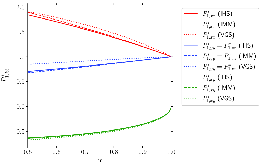
Figure 2: Plot of the (reduced) elements of the pressure tensor $P_{1,k\ell}^{*}$ as functions of the (common) coefficient of restitution $\alpha_{22}=\alpha_{12}\equiv\alpha$ for a three-dimensional single system ($d=3$) in the case $\sigma_{1}/\sigma_{2}=m_{1}/m_{2}=0.5$. The solid lines are the approximate results derived for IHS from the leading Sonine approximation, the dashed lines correspond to the results obtained for IMM, and the dotted lines refer to the results of the VGS kinetic model.

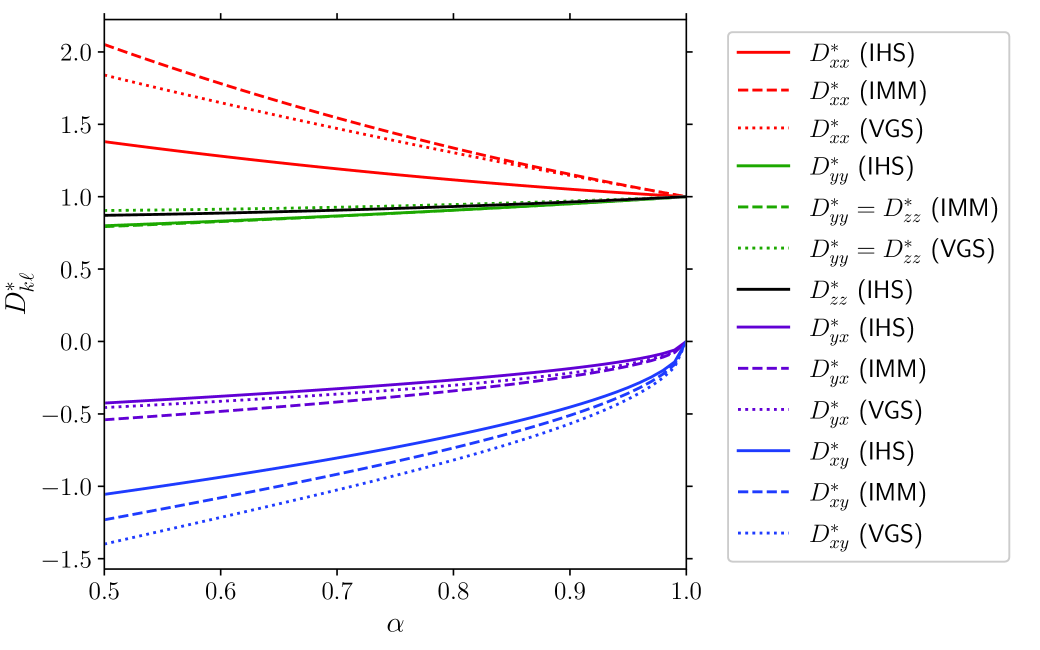
Figure 3: Plot of the (reduced) elements $D_{xx}^{*}$, $D_{yy}^{*}$, $D_{zz}^{*}$, $D_{xy}^{*}$, and $D_{yx}^{*}$ as functions of the (common) coefficient of restitution $\alpha$ for a three-dimensional system in the case $\sigma_{1}/\sigma_{2}=1$ and $m_{1}/m_{2}=0.5$. The solid lines are the approximate results derived for IHS from the leading Sonine approximation, the dashed lines correspond to the results obtained for IMM, and the dotted lines refer to the results of the VGS kinetic model. Note that $D_{yy}^{*}=D_{zz}^{*}$ in the results obtained from IMM and the kinetic model.

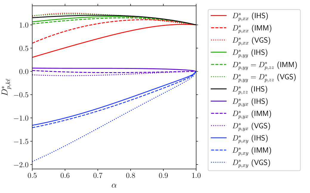
Figure 4: Plot of the (reduced) elements $D_{p,xx}^{*}$, $D_{p,yy}^{*}$, $D_{p,zz}^{*}$, $D_{p,xy}^{*}$, and $D_{p,yx}^{*}$ as functions of the (common) coefficient of restitution $\alpha$ for a three-dimensional system in the case $\sigma_{1}/\sigma_{2}=1$ and $m_{1}/m_{2}=0.5$. The solid lines are the approximate results derived for IHS from the leading Sonine approximation, the dashed lines correspond to the results obtained for IMM, and the dotted lines refer to the results of the VGS kinetic model. Note that $D_{p,yy}^{*}=D_{p,zz}^{*}$ in the results obtained from IMM and the kinetic model.

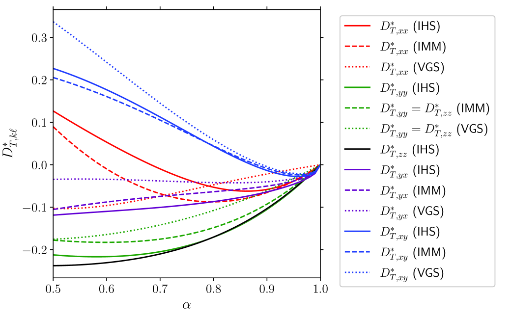
Figure 5: Plot of the (reduced) elements $D_{T,xx}^{*}$, $D_{T,yy}^{*}$, $D_{T,zz}^{*}$, $D_{T,xy}^{*}$, and $D_{T,yx}^{*}$ as functions of the (common) coefficient of restitution $\alpha$ for a three-dimensional system in the case $\sigma_{1}/\sigma_{2}=1$ and $m_{1}/m_{2}=0.5$. The solid lines are the approximate results derived for IHS from the leading Sonine approximation, the dashed lines correspond to the results obtained for IMM, and the dotted lines refer to the results of the VGS kinetic model. Note that $D_{T,yy}^{*}=D_{T,zz}^{*}$ in the results obtained from IMM and the kinetic model.

In this section, we want to compare the results obtained from both the Boltzmann equation for IMM and the VGS kinetic model with those previously derived from the IHS Garzó (2002, 2007). In dimensionless form, the rheological properties and the diffusion coefficients of the system (granular gas plus tracer particles) depend on five quantities: the diameter $\sigma_{1}/\sigma_{2}$ and mass $m_{1}/m_{2}$ ratios, the coefficients of restitution $\alpha_{22}$ and $\alpha_{12}$, and the dimensionality $d$ of the system. Thus, given that the parameter space of the system is large, henceforth we consider a three-dimensional gas ($d=3$) and a common coefficient of restitution $\alpha_{22}=\alpha_{12}\equiv\alpha$. This reduces the parameter space to three quantities: $\sigma_{1}/\sigma_{2}$, $m_{1}/m_{2}$, and $\alpha$.

First, we consider the rheological properties. In the case of the excess granular gas, figure 1 shows $P_{2,k\ell}^{*}$ versus $\alpha_{22}$. We have also included computer simulation results Montanero and Garzó (2002) obtained by numerically solving the (inelastic) Boltzmann equation for IHS by means of the direct simulation Monte Carlo (DSMC) method Bird (1994). Comparing the three approaches, we see that the quantitative discrepancies between the VGS model’s theoretical predictions and the approximate IHS results are larger than those found for the IMM results. In fact, the theoretical results for IHS and IMM disagree very little; this difference increases slightly with inelasticity. Additionally, we observe excellent agreement between the Boltzmann theory for both interaction models and Monte Carlo simulations, even in the case of strong dissipation. Similar conclusions are reached for the reduced pressure tensor, $P_{1,k\ell}^{*}$. Figure 2 illustrates this behavior, showing the dependence of $P_{1,k\ell}^{*}$ on $\alpha$ for the case $\sigma_{1}/\sigma_{2}=1$ and $m_{1}/m_{2}=0.5$. The good agreement between the IHS and IMM results is apparent again, especially in the case of the shear stress $P_{1,xy}^{*}$, which is the most relevant rheological property in a shear flow problem as it defines the non-Newtonian shear viscosity. Although the VGS model predictions are good qualitatively, they exhibit larger discrepancies with the IHS results than the IMM predictions.

We analyze now the dependence of the diffusion coefficients $T_{k\ell}\equiv\left\{D_{k\ell},D_{p,k\ell},D_{T,k\ell}\right\}$ on the (common) coefficient of restitution $\alpha$. According to the results derived in sections IV and V, $T_{xz}=T_{zx}=T_{yz}=T_{zy}=0$ in agreement with the symmetry of the shearing field applied to the system. Thus, in a three-dimensional gas, there are five relevant elements of the tensors $T_{k\ell}$: the three diagonal ($T_{xx}$, $T_{yy}$, and $T_{zz}$) and two off-diagonal elements ($T_{xy}$ and $T_{yx}$). The results obtained here for IMM and from the kinetic model show that in general $T_{xx}\neq T_{yy}=T_{zz}$ and $T_{xy}\neq T_{yx}$. However, in the case of IHS, the approximate results derived in Ref. Garzó (2007) show that $T_{yy}\neq T_{zz}$ although the difference between both elements is in general very small.

Given that we are interested in this paper to assess the dependence of the coefficients $T_{k\ell}$ on inelasticity, we have scaled them with respect to their elastic values except in the case of $D_{T,k\ell}$ since this coefficient vanishes for elastic collisions. Thus, we define the dimensionless coefficients $D_{k\ell}^{*}=D_{k\ell}/D^{\text{el}}$ and $D_{p,k\ell}^{*}=D_{p,k\ell}/D_{p}^{\text{el}}$ while $D_{T,k\ell}^{*}=D_{T,k\ell}/(x_{1}T/m_{2}\nu)$. The effective collision frequency $\nu=\nu_{\text{M},22}$ for IMM, $\nu=\nu_{22}$ for the VGS model, and $\nu=(2/(d+2))\nu_{\text{M},22}$ for IHS. The relevant elements of $D_{k\ell}^{*}$, $D_{p,k\ell}^{*}$, and $D_{T,k\ell}^{*}$ are plotted in figures 3, 4, and 5, respectively, as functions of $\alpha$ for the mixture $\sigma_{1}/\sigma_{2}=1$ and $m_{1}/m_{2}=0.5$. As expected, we observe that in general the influence of inelasticity on mass transport is quite significant regardless of the approximation used. Additionally, the anisotropy of the system (as measured by the differences $|T_{xx}-T_{yy}|$ and $|T_{zz}-T_{yy}|$) is much important in the shear flow $xy$-plane. In fact, while $T_{zz}-T_{yy}=0$ for IMM and kinetic model results, we observe that $T_{zz}\simeq T_{yy}$ for IHS. With respect to the comparison between IHS, IMM, and kinetic model, it is quite apparent that although the predictions of the kinetic model reproduce qualitatively well the results obtained for IHS, significant discrepancies between both approaches are found for strong dissipation. As occurs for the rheology, the agreement between IMM and IHS is better than the one found between IHS and the kinetic model. In fact, the good agreement obtained here between IHS and IMM can justify the use of IMM as a reliable model to unveil in a clean way the effect of inelasticity on transport in real granular flows.

VII Thermal diffusion segregation

The knowledge of the diffusion transport coefficients allows us to apply the present theoretical results to the problem of segregation of tracer particles in a sheared granular gas. Segregation of dissimilar species in a granular mixture is likely one of the most relevant problems in granular flows not only from a fundamental point of view, but also from a more practical perspective. The problem was already studied in the context of IHS Garzó and Vega Reyes (2010). Our objective here is to revisit the problem by employing the results derived for IMM and from the VGS kinetic model.

Within the different mechanisms involved in the segregation, thermal diffusion segregation is perhaps one of the most studied in the literature Grew and Ibbs (1952); Kincaid et al. (1987). Thermal diffusion is produced by a thermal gradient which induces a relative motion within a mixture. This motion generates diffusion processes due to the concentration gradients created by the presence of thermal gradient. A steady state is achieved when thermal diffusion is balanced by the mixing effect coming from ordinary diffusion.

However, due to the anisotropy in velocity space induced by the shear flow, a complete description of the segregation problem requires to introduce a thermal diffusion tensor to characterize segregation in the different directions. Here, as in Ref. Garzó and Vega Reyes (2010), for the sake of simplicity we consider a situation where the temperature gradient is perpendicular to the shear flow plane. Thus, for a three-dimensional system, $\partial_{x}T=\partial_{y}T=0$ but $\partial_{z}T\neq 0$. Additionally, since we are interested in a situation where the hydrodynamic equations (52)–(54) admit a steady solution, we also assume that $\delta\mathbf{U}=\mathbf{0}$. Under these conditions, the amount of segregation parallel to the $z$-axis can be measured by the thermal diffusion factor $\Lambda_{z}$ defined as

$$-\Lambda_{z}\frac{\partial\ln T}{\partial z}=\frac{\partial\ln x_{1}}{\partial z}.$$ (95)

If we assume that the thermal gradient is directed downwards ($\partial_{z}T<0$), when $\Lambda_{z}>0$ ($\Lambda_{z}<0$) the tracer particles tend to accumulate near the cold (hot) wall since $\partial_{z}\ln x_{1}>0$ ($\partial_{z}\ln x_{1}<0$).

Let us write $\Lambda_{z}$ in terms of the pressure tensors $P_{zz}$ and $P_{1,zz}$ as well as the diffusion coefficients $D_{zz}$, $D_{p,zz}$ and $D_{T,zz}$. First, when only gradients along the $z$-axis exist, the momentum balance equation (53) yields

$$\frac{\partial P_{zz}}{\partial z}=0.$$ (96)

Since $P_{zz}=pP_{zz}^{*}(a^{*})$, then

$$\frac{\partial P_{zz}}{\partial z}=\frac{\partial p}{\partial z}\left(1-a^{*}\partial_{a^{*}}\right)P_{zz}^{*}+\frac{p}{2T}\frac{\partial T}{\partial z}a^{*}(\partial_{a^{*}}P_{zz}^{*}),$$ (97)

where $\partial_{a^{*}}P_{zz}^{*}=\partial_{a^{*}}P_{yy}^{*}\equiv\Delta_{yy}$ is given by Eq. (128). Using Eqs. (96) and (97), one gets a relationship between $\partial_{z}p$ and $\partial_{z}T$:

$$\frac{\partial\ln p}{\partial z}=-\frac{1}{2}\frac{a^{*}(\partial_{a^{*}}P_{zz}^{*})}{P_{zz}^{*}-a^{*}(\partial_{a^{*}}P_{zz}^{*})}\frac{\partial\ln T}{\partial z}.$$ (98)

In addition, according to the balance equation (52), in the steady state with $\delta\mathbf{U}=\mathbf{0}$ then $j_{1,z}^{(1)}=0$. The constitutive equation for $j_{1,z}^{(1)}$ is

$$j_{1,z}^{(1)}=-m_{1}D_{zz}\partial_{z}x_{1}-\frac{m_{2}}{T}D_{p,zz}\partial_{z}p-\frac{\rho}{T}D_{T,zz}\partial_{z}T.$$ (99)

The condition $j_{1,z}^{(1)}=0$ leads to

$$\frac{\partial\ln x_{1}}{\partial z}=-\frac{\rho}{m_{1}x_{1}}\left(\frac{D_{p,zz}}{D_{zz}}\frac{\partial\ln p}{\partial z}+\frac{D_{T,zz}}{D_{zz}}\frac{\partial\ln T}{\partial z}\right)=-\Bigg[(1-\mu)\frac{D_{p,zz}^{*}}{D_{zz}^{*}}\frac{\partial\ln p}{\partial z}+\Omega^{\text{el}*}\frac{D_{T,zz}^{*}}{D_{zz}^{*}}\frac{\partial\ln T}{\partial z}\Bigg].$$ (100)

Here, $\mu=m_{1}/m_{2}$ is the mass ratio and $\Omega^{\text{el}*}=\Omega^{\text{el}}/\nu$, where the value of $\nu$ depends on the approach followed.

From Eqs. (98) and (100) one easily gets the expression of the thermal diffusion factor $\Lambda_{z}$ as

$$\Lambda_{z}=\frac{\Omega^{\text{el}*}D_{T,zz}^{*}-\frac{1}{2}(1-\mu)a^{*}\Delta_{yy}\left(P_{zz}^{*}-a^{*}\Delta_{yy}\right)^{-1}D_{p,zz}^{*}}{D_{zz}^{*}}.$$ (101)

The condition $\Lambda_{z}=0$ gives the criterion for the upwards/downwards segregation transition.

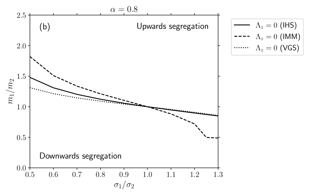
Figure 6: (a) Phase diagram for segregation in the $\left\{\sigma_{1}/\sigma_{2},m_{1}/m_{2}\right\}$ plane for a three-dimensional system ($d=3$) with $\alpha=0.9$. (b) Phase diagram for segregation in the $\left\{\sigma_{1}/\sigma_{2},m_{1}/m_{2}\right\}$ plane for a three-dimensional system ($d=3$) with $\alpha=0.8$.

In accordance to Eq. (82) the diffusion coefficient $D_{zz}^{*}$ is positive. As a consequence, the marginal segregation curve ($\Lambda_{z}=0$) is obtained from the condition

$$\Omega^{\text{el}*}D_{T,zz}^{*}-\frac{1}{2}(1-\mu)a^{*}\Delta_{yy}\left(P_{zz}^{*}-a^{*}\Delta_{yy}\right)^{-1}D_{p,zz}^{*}=0.$$ (102)

For elastic collisions ($\alpha_{22}=\alpha_{12}=1$), $D_{T,zz}^{*}=0$ and Eq. (42) for IMM or Eq. (87) for the VGS kinetic model yields $a^{*}=0$. Thus, the condition (102) is trivially satisfied for any value of the mass and diameter ratios and so, no segregation occurs in this limiting case as expected. On the other hand, for inelastic collisions but the particles are mechanically equivalent, $D_{p,k\ell}^{*}=D_{T,k\ell}^{*}=0$ and so, $\Lambda_{z}=0$ for any value of the coefficient of restitution. This is the expected result since both species are indistinguishable.

For inelastic collisions, the zero contour of $\Lambda_{z}$ exhibits a complex nonlinear dependence on the parameter space of the system. Thus, as did in section VI, for the sake of simplicity we take a three-dimensional granular gas ($d=3$) in the case of a common coefficient of restitution ($\alpha_{22}=\alpha_{12}\equiv\alpha$). The marginal segregation curve $\Lambda_{z}=0$ separates regions of $\Lambda_{z}>0$ (upwards segregation) and $\Lambda_{z}<0$ (downwards segregation). At a fixed value of $\alpha$, the points lying on the zero contour correspond to values of the diameter and mass ratios for which the intruder does not segregate in a sheared granular gas.

As an illustration, figure 6 shows the phase diagram in the $\left(\sigma_{1}/\sigma_{2},m_{1}/m_{2}\right)$-plane for two different values of the (common) coefficient of restitution $\alpha$. We compare the theoretical predictions for the marginal segregation curve $\Lambda_{z}=0$ obtained previously for IHS in Ref. Garzó and Vega Reyes (2010) with those derived here for IMM and from the VGS kinetic model. As previously mentioned, all curves pass through the point $(1,1)$ because it corresponds to the limiting case of mechanically equivalent particles. The three approaches show that, for $\sigma_{1}<\sigma_{2}$, the main effect of inelasticity (or equivalently, the reduce shear rate $a^{*}$) is to enlarge the size of the downwards segregation region. The opposite occurs when the tracer particles are larger than the particles of the granular gas. In general, we see that the tracer particles tend to move toward hotter regions since upwards segregation occupies most of the system’s parameter space. Regarding the comparison of the three approaches, the results derived from IMM qualitatively agree well with the IHS results. Surprisingly, however, the segregation results obtained from the VGS model agree better with the IHS results than with the IMM results. This good agreement is especially noticeable when $\sigma_{1}>\sigma_{2}$.

VIII Concluding remarks

In this paper, we have analyzed the diffusion of tracer particles immersed in a sheared granular gas. Under these conditions, the mass flux $\mathbf{j}_{1}^{(1)}$ is defined in terms of the tracer diffusion tensor $D_{k\ell}$ (which couples $\mathbf{j}_{1}^{(1)}$ with the concentration gradient $\nabla x_{1}$), the pressure diffusion tensor $D_{p,k\ell}$ (which couples $\mathbf{j}_{1}^{(1)}$ with the pressure gradient $\nabla p$), and the thermal diffusion tensor $D_{T,k\ell}$ (which couples $\mathbf{j}_{1}^{(1)}$ with the temperature gradient $\nabla T$). These tensorial quantities were evaluated years ago in the context of the Boltzmann equation for IHS Garzó (2002, 2007). However, due to the intricate mathematical structure of the Boltzmann collision operator for IHS, the results obtained in Refs. Garzó (2002, 2007) involve several (uncontrolled) approximations at different stages of the derivation. Here, we revisit this problem by considering two different, complementary approaches that allow us to achieve exact results. First, we maintain the structure of the Boltzmann collision operators but consider a different interaction model: the so-called IMM, in which the collision rate of colliding spheres is independent of their relative velocity. This simplification enables us to obtain exact expressions for the rheological properties of the system (granular gas plus tracer particles), as well as the diffusion tensors. As a second approach, we keep the IHS interaction model but replace the true Boltzmann collision operators with simpler mathematical terms that retain their relevant physical properties. In this context, we consider the VGS kinetic model Vega Reyes et al. (2007) proposed years ago for granular mixtures.

As in Ref. Garzó (2007) for IHS, the diffusion tensors are obtained by solving the Boltzmann equation (or the VGS model) for tracer particles using a generalization of the Chapman–Enskog method Chapman and Cowling (1970) for far-from-equilibrium states. Since the granular gas is subjected to a strong shear rate, non Newtonian effects are relevant for finite inelasticity. Thus, the reference state (the zeroth-order distribution $f_{1}^{(0)}$) in the perturbation method is the shear flow distribution, not the local equilibrium distribution. Additionally, since collisional cooling cannot compensate for viscous heating locally, $f_{1}^{(0)}$ is in general a time-dependent distribution even when the gas is slightly perturbed from the USF. Once the linear integral equations verifying the diffusion tensors are obtained, we restrict to steady state conditions and so, the reduced shear rate $a^{*}$ is coupled to the coefficient of restitution $\alpha_{22}$ which characterizes the inelasticity of grain-grain collisions. The consideration of the steady state allows us to achieve analytical, exact expressions for $D_{k\ell}$, $D_{p,k\ell}$, and $D_{T,k\ell}$. These tensors depend nonlinearly on the diameter ratio, $\sigma_{1}/\sigma_{2}$, the mass ratio, $m_{1}/m_{2}$, and the coefficients of restitution $\alpha_{22}$ and $\alpha_{12}$ (which characterizes the inelasticity of tracer-grain collisions).

A comparison of the exact theoretical results of the IMM and VGS models with the approximate IHS results generally shows good qualitative agreement. At a more quantitative level, we observe excellent agreement in some cases (e.g., rheological properties) and reasonably good agreement in others (e.g., diffusion tensors), especially in the case of IMM. It is quite apparent that to confirm the reliability of the predictions offered by IMM and VGS model one should compare them with computer simulation results for IHS. At the level of rheology, the results reported here (see figure 1) and in Ref. Goldhirsch (2003) for IMM clearly demonstrate the accuracy of this interaction model to capture the dependence of the pressure tensors on the coefficients of restitution. The lack of simulation data for the diffusion coefficients in the low-density regime prevents a comparison between theory and simulation. We hope that this paper will encourage simulators to perform simulations and confirm the results reported here.

As a nice application of the results exposed in this paper, the segregation of tracer particles in a sheared granular gas has been analyzed. The relative motion of the tracers with respect to the particles of the gas is caused by the presence of a temperature gradient. Here, for the sake of simplicity, we have assumed that the thermal gradient $\partial_{z}T$ is perpendicular to the shear flow $xy$-plane. Under these conditions, the amount of segregation in the $z$-direction is measured by the thermal diffusion factor $\Lambda_{z}$, defined in Eq. (95). The condition of zero thermal diffusion ($\Lambda_{z}=0$) gives the segregation criterion for the transition from upwards segregation (regions where $\Lambda_{z}>0$) to downwards segregation (regions where $\Lambda_{z}<0$). A comparison with previous results obtained for IHS Garzó and Vega Reyes (2010) (see figure 6) shows reasonable agreement in general, especially for the VGS model when the tracer particles are larger than the granular gas particles.

In conclusion, the results found here give evidence of the accuracy of both IMM and the VGS kinetic model for studying far-from-equilibrium situations in granular flows, where using the original Boltzmann equation for IHS turns out to be quite intricate. Additionally, using a kinetic model instead of the Boltzmann equation for IHS and/or IMM allows us to obtain the explicit forms of the velocity distribution functions. This is likely one of the main advantages of starting from a kinetic model rather than the true Boltzmann kinetic equation.

Appendix A Linear stability analysis of the steady state solutions to USF

In this Appendix, we want to see whether the steady state solutions (41)–(50) to the pressure tensors are (linearly) stable. We consider first the time evolution equation for the pressure tensor of the excess granular gas. The three relevant independent equations for $P_{2,k\ell}$ are given by

$$\partial_{t}p+\zeta_{2}p+\frac{2a}{d}P_{2,xy}=0,\quad\partial_{t}P_{2,xy}+\nu_{\eta}P_{2,xy}+aP_{2,yy}=0,$$ (103)

$$\partial_{t}P_{2,yy}+\nu_{\eta}P_{2,yy}-\left(\nu_{\eta}-\zeta_{2}\right)P_{2,yy}=0,$$ (104)

where $\nu_{\eta}=\nu_{\text{M},22}\nu_{\eta}^{*}$ and $p\simeq p_{2}=n_{2}T_{2}$. In terms of the dimensionless quantities, $P_{2,k\ell}^{*}(t)=P_{2,k\ell}(t)/n_{2}T(t)$, $a^{*}(t)=a/\nu_{\text{M},22}(t)$ and

$$\tau(t)=\int_{0}^{t}dt^{\prime}\;\nu_{\text{M},22}(t^{\prime}),$$ (105)

Eqs. (103) and (104) become

$$2\partial_{\tau}\ln a^{*}=\zeta_{2}^{*}+\frac{2}{d}a^{*}P_{2,xy}^{*},$$ (106)

$$\partial_{\tau}P_{2,xy}^{*}=-a^{*}P_{2,yy}^{*}-P_{2,xy}^{*}\Big(\nu_{\eta}^{*}-\zeta_{2}^{*}-\frac{2}{d}a^{*}P_{2,xy}^{*}\Big),$$ (107)

$$\partial_{\tau}P_{2,yy}^{*}=-P_{2,yy}^{*}\Big(\nu_{\eta}^{*}-\zeta_{2}^{*}-\frac{2}{d}a^{*}P_{2,xy}^{*}\Big)+\nu_{\eta}^{*}-\zeta_{2}^{*},$$ (108)

The variable $\tau$ is the dimensionless time measured as the average collision number. A steady solution of Eqs. (106)–(108) is given by Eqs. (41) and (42). To carry out a linear stability analysis of these steady solutions, we look for solutions to the set (106)–(108) given by

$$a^{*}(\tau)=a_{s}^{*}+\delta a^{*}(\tau),\quad P_{2,xy}^{*}(\tau)=P_{2xy,s}^{*}+\delta P_{2,xy}^{*}(\tau),\quad P_{2,yy}^{*}(\tau)=P_{2yy,s}^{*}+\delta P_{2,yy}^{*}(\tau),$$ (109)

where the subscript $s$ means that the quantities are evaluated in the steady state. Substituting the identities (109) into Eqs. (106)–(108) and neglecting nonlinear terms in the perturbations, one gets

$$\partial_{\tau}\left(\begin{array}[]{c}\delta a_{s}^{*}\\ \delta P_{2,xy}^{*}\\ a_{s}^{*}\delta P_{2,yy}^{*}\end{array}\right)=-\mathsf{L}\cdot\left(\begin{array}[]{c}\delta a^{*}\\ \delta P_{2,xy}^{*}\\ a_{s}^{*}\delta P_{2,yy}^{*}\end{array}\right),$$ (110)

where $\mathsf{L}$ is the square matrix

$$\mathsf{L}=\left(\begin{array}[]{ccc}\frac{\zeta_{2}^{*}}{2}&-\frac{\zeta_{2}^{*}\nu_{\eta}^{*2}}{2(\nu_{\eta}^{*}-\zeta_{2}^{*})}&0\\ \left(\frac{\nu_{\eta}^{*}-\zeta_{2}^{*}}{\nu_{\eta}^{*}}\right)^{2}&\nu_{\eta}^{*}+\zeta_{2}^{*}&1\\ \frac{(\nu_{\eta}^{*}-\zeta_{2}^{*})\zeta_{2}^{*}}{\nu_{\eta}^{*}}&-\zeta_{2}^{*}\nu_{\eta}^{*}&\nu_{\eta}^{*}\end{array}\right).$$ (111)

The time evolution of the deviations from the steady solution is governed by the three eigenvalues of the matrix $\mathsf{L}$. If the real parts of those eigenvalues are positive the steady solution is linearly stable, while is unstable otherwise. The eigenvalues are determined from the solution of the secular equation

$$\det\left(L_{k\ell}-\ell\delta_{k\ell}\right)=0.$$ (112)

The solution to Eq. (112) leads to a real eigenvalue $\ell_{1}$ and a pair of complex conjugate eigenvalues $\ell_{2}$ and $\ell_{3}$. As for IHS Santos et al. (2004), the results show that $\text{Re}(\lambda_{i})>0$ ($i=1,2,3$) for any value of $\alpha_{22}$. This means that the steady USF solution for the excess granular is linearly stable, and the characteristic relaxation time (measured by the number of collisions) is $\ell_{1}^{-1}$. As an illustration, figure 7 shows the dependence of $\ell_{1}$ and of the real part of $\ell_{2,3}$ for a three-dimensional granular gas ($d=3$). Note that $\ell_{1}\to 0$ in the elastic limit $\alpha_{22}\to 1$. This is a consequence that for elastic collisions $a^{*}\to 0$.

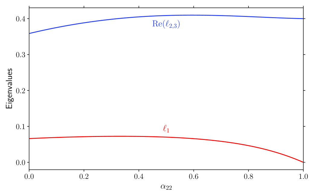
Figure 7: Plot of the eigenvalue $\ell_{1}$ and of the real part of $\ell_{2,3}$ as a function of the coefficient of restitution $\alpha_{22}$ for a three-dimensional system.

We consider now the (linear) stability of the steady solution to the set of time evolution equations associated with $\gamma(t)$, $P_{1,xy}(t)$ and $P_{1,yy}(t)$. Since we have previously shown that the perturbations $(\delta a^{*},\delta P_{2,xy}^{*},\delta P_{2,yy}^{*})$ tend to zero for sufficiently long times, we assume hence that $a^{*}\equiv\text{const.}$, $P_{2,xy}^{*}\equiv\text{const.}$ and $P_{2,yy}^{*}\equiv\text{const.}$ in the evolution equations of $\gamma(t)$, $P_{1,xy}(t)$ and $P_{1,yy}(t)$. In terms of the variable $\tau$, the set of equations for $\gamma$, $P_{1,xy}$ and $P_{1,yy}$ is

$$\partial_{\tau}\gamma=-\frac{2}{d}a^{*}P_{1,xy}^{*}-\zeta_{1}^{*}\gamma,$$ (113)

$$\partial_{\tau}P_{1,yy}^{*}=Y+X_{0}P_{1,yy}^{*}+XP_{2,yy}^{*},$$ (114)

$$\partial_{\tau}P_{1,xy}^{*}+a^{*}P_{1,yy}^{*}=X_{0}P_{1,xy}^{*}+XP_{2,yy}^{*},$$ (115)

where the quantities $Y$, $X_{0}$ and $X$ are defined by Eqs. (45) and (47), respectively. As in the case of the excess granular gas, we want to solve the set of Eqs. (113)–(115) by assuming small deviations from the steady state solution. Thus, we write

$$\gamma(\tau)=\gamma_{s}+\delta\gamma(\tau),\quad P_{1,yy}^{*}(\tau)=P_{1yy,s}^{*}+\delta P_{1,yy}^{*}(\tau),\quad P_{1,xy}^{*}(\tau)=P_{1xy,s}^{*}+\delta P_{1,xy}^{*}(\tau).$$ (116)

In the linear order in the perturbations,

$$\zeta_{1}^{*}=\zeta_{1s}^{*}+\overline{\zeta}_{1}\delta\gamma,\quad Y=Y_{s}+\overline{Y}\delta\gamma,\quad X_{0}=X_{0s}+\overline{X}_{0}\delta\gamma,\quad X=X_{s}+\overline{X}\delta\gamma,$$ (117)

where $\zeta_{1s}^{*}$, $Y_{s}$, $X_{0s}$, and $X_{s}$ refer to the values of these quantities in the steady state and

$$\overline{\zeta}_{1}=\frac{\sqrt{2}}{d}\left(\frac{\sigma_{12}}{\sigma_{2}}\right)^{d-1}\mu_{21}(1+\alpha_{12})\Bigg\{\frac{(1+\theta_{s}^{-1})^{-1/2}}{2\mu}\left[1-\frac{\mu_{21}}{2}(1+\alpha_{12})(1+\theta_{s})\right]$$

$$+\frac{\mu_{21}^{2}}{2\mu_{12}}\theta_{s}^{2}(1+\theta_{s}^{-1})^{1/2}(1+\alpha_{12})\Bigg\},$$ (118)

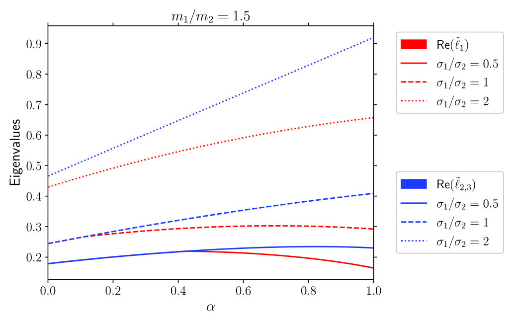
Figure 8: Plot of the real parts of the eigenvalues $\widetilde{\ell}_{i}$ ($i=1,2,3$) as functions of the (common) coefficient of restitution $\alpha_{22}=\alpha_{12}\equiv\alpha$ for the mass ratio $m_{1}/m_{2}=1.5$ and different values of the diameter ratio $\sigma_{1}/\sigma_{2}$.

$$\overline{Y}=\frac{3}{2\sqrt{2}}\left(\frac{\sigma_{12}}{\sigma_{2}}\right)^{d-1}\frac{\mu_{21}^{2}}{(d+2)}(1+\alpha_{12})^{2}(1+\theta_{s}^{-1})^{1/2},$$ (119)

$$\overline{X}_{0}=-\frac{1}{\sqrt{2}d(d+2)}\left(\frac{\sigma_{12}}{\sigma_{2}}\right)^{d-1}\frac{\mu_{21}^{2}}{\mu_{12}}(1+\theta_{s}^{-1})^{-1/2}(1+\alpha_{12})\left[d+2-\mu_{21}(1+\alpha_{12})\right],$$ (120)

$$\overline{X}=\frac{1}{\sqrt{2}d(d+2)}\left(\frac{\sigma_{12}}{\sigma_{2}}\right)^{d-1}\mu_{21}^{2}(1+\theta_{s}^{-1})^{-1/2}(1+\alpha_{12})^{2}.$$ (121)

Substitution of Eqs. (116) and (117) into Eqs. (113)–(115) and neglecting nonlinear terms in the perturbations, after some algebra one gets the set of linear differential equations:

$$\partial_{\tau}\left(\begin{array}[]{c}\delta\gamma\\ \delta P_{1,yy}^{*}\\ \delta P_{1,xy}^{*}\end{array}\right)=-\widetilde{\mathsf{L}}\cdot\left(\begin{array}[]{c}\delta\gamma\\ \delta P_{1,yy}^{*}\\ \delta P_{1,xy}^{*}\end{array}\right),$$ (122)

where $\widetilde{\mathsf{L}}$ is the square matrix

$$\widetilde{\mathsf{L}}=\left(\begin{array}[]{ccc}\zeta_{1s}^{*}+\gamma_{s}\overline{\zeta}_{1}&0&\frac{2}{d}a_{s}^{*}\\ -\left(\overline{Y}+\overline{X}_{0}P_{1,yy,s}^{*}+\overline{X}P_{yy,s}^{*}\right)&-X_{0s}&0\\ -\left(\overline{X}_{0}P_{1,xy,s}^{*}+\overline{X}P_{yy,s}^{*}\right)&a_{s}^{*}&-X_{0s}\end{array}\right).$$ (123)

The eigenvalues of the matrix $\widetilde{\mathsf{L}}$ are the roots of the secular equation

$$\det\left(\widetilde{L}_{k\ell}-\widetilde{\ell}\delta_{k\ell}\right)=0.$$ (124)

If the real parts of the eigenvalues $\widetilde{\ell}$ are always positive for any value of the set $(\alpha_{22},\alpha_{12},m_{1}/m_{2},\sigma_{1}/\sigma_{2})$ then the steady USF solution for the pressure tensor $P_{1,ij}^{*}$ is linearly stable.

A systematic analysis of the dependence of $\text{Re}(\;\widetilde{\ell}_{i})$ ($i=1,2,3$) on the parameter space shows that the real parts of the eigenvalues are always positive. As an illustration, figures 9 and 8 show the $\alpha$-dependence of $\text{Re}(\;\widetilde{\ell}_{i})$; being quite apparent that their real parts are positive.

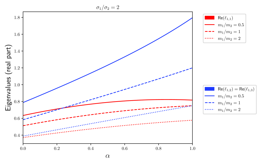
Figure 9: Plot of the real parts of the eigenvalues $\widetilde{\ell}_{i}$ ($i=1,2,3$) as functions of the (common) coefficient of restitution $\alpha_{22}=\alpha_{12}\equiv\alpha$ for the diameter ratio $\sigma_{1}/\sigma_{2}=2$ and different values of the mass ratio $m_{1}/m_{2}$.

Appendix B Behavior of the zeroth-order pressure tensors near the steady state

In this Appendix we give the expressions of the derivatives of the zeroth-order pressure tensors $P_{k\ell}^{*}$ and $P_{1,k\ell}^{*}$ with respect to $a^{*}$ near the steady state. We consider first IMM where the (dimensionless) elements of the pressure tensor $P_{k\ell}^{*}$ obey the equation

$$-\left(\frac{2}{d}a^{*}P_{xy}^{*}+\zeta^{*}\right)\left(1-\frac{1}{2}a^{*}\frac{\partial}{\partial a^{*}}\right)P_{k\ell}^{*}+a_{k\mu}^{*}P_{\ell\mu}^{*}+a_{\ell\mu}^{*}P_{k\mu}^{*}=-\left[\nu_{\eta}^{*}P_{k\ell}^{*}+\left(\zeta^{*}-\nu_{\eta}^{*}\right)\delta_{k\ell}\right],$$ (125)

where in the tracer limit $P_{2,k\ell}^{*}\simeq P_{k\ell}^{*}$ and $\zeta_{2}^{*}\simeq\zeta^{*}$. From Eq. (125), one gets the set of equations

$$\frac{\partial P_{yy}^{*}}{\partial a^{*}}=\frac{2(\nu_{\eta}^{*}-\zeta^{*})-2P_{yy}^{*}\left(\nu_{\eta}^{*}-\zeta^{*}-\frac{2}{d}a^{*}P_{xy}^{*}\right)}{a^{*}\left(\frac{2}{d}a^{*}P_{xy}^{*}+\zeta^{*}\right)},$$ (126)

$$\frac{\partial P_{xy}^{*}}{\partial a^{*}}=\frac{-2P_{yy}^{*}a^{*}-2P_{xy}^{*}\left(\nu_{\eta}^{*}-\zeta^{*}-\frac{2}{d}a^{*}P_{xy}^{*}\right)}{a^{*}\left(\frac{2}{d}a^{*}P_{xy}^{*}+\zeta^{*}\right)}.$$ (127)

As expected, the numerators and denominators of Eqs. (126) and (127) vanish in the steady state $[(2/d)a^{*}P_{xy}^{*}+\zeta^{*}=0]$. As in the case of IHS Garzó (2007), the steady-state limit of Eqs. (126) and (127) can be evaluated by means of l’Hopital’s rule. In this case, one achieves the results

$$\Delta_{yy}=4P_{yy}^{*}\frac{a^{*}\Delta_{xy}+P_{xy}^{*}}{2a^{*2}\Delta_{xy}+d\left(2\nu_{\eta}^{*}-\zeta^{*}\right)},$$ (128)

where $\Delta_{yy}\equiv\left(\partial P_{yy}^{*}/\partial a^{*}\right)_{s}$ and $\Delta_{xy}\equiv\left(\partial P_{xy}^{*}/\partial a^{*}\right)_{s}$ is the real root of the cubic equation

$$2a^{*4}\Delta_{xy}^{3}+4da^{*2}\nu_{\eta}^{*}\Delta_{xy}^{2}+\frac{d^{2}}{2}\left(4\nu_{\eta}^{*2}+6\zeta^{*}\nu_{\eta}^{*}-3\zeta^{*2}\right)\Delta_{xy}$$

$$+d^{2}\left(\nu_{\eta}^{*}-\zeta^{*}\right)\nu_{\eta}^{*-2}\left(\zeta^{*2}-5\zeta^{*}\nu_{\eta}^{*}+2\nu_{\eta}^{*2}\right)=0.$$ (129)

In the above equations, it is understood that all the quantities are computed in the steady state.

We consider now the derivatives of the elements $P_{1,k\ell}^{*}$ with respect to $a^{*}$. They verify the time dependent equation

$$-\left(\frac{2}{d}a^{*}P_{xy}^{*}+\zeta^{*}\right)\left(1-\frac{1}{2}a^{*}\frac{\partial}{\partial a^{*}}\right)P_{1,k\ell}^{*}+a_{k\mu}^{*}P_{1,\ell\mu}^{*}+a_{l\mu}^{*}P_{1,k\mu}^{*}=Y\delta_{k\ell}+X_{0}P_{1,k\ell}^{*}+XP_{k\ell}^{*},$$ (130)

where we recall that the quantities $Y$, $X_{0}$ and $X$ for IMM are defined by Eqs. (45) and (47), respectively. The derivatives of $\partial_{a^{*}}P_{1,yy}^{*}$, $\partial_{a^{*}}P_{1,xy}^{*}$, and $\partial_{a^{*}}\gamma$ can be easily obtained from the results derived for IHS in Ref. Garzó (2007) by replacing the expressions of the quantities $Y$, $X_{0}$, and $X$ of IHS by their corresponding counterparts for IMM given by Eqs. (45) and (47), respectively. Thus, the expressions of the derivatives $\partial_{a^{*}}P_{1,xy}^{*}$ and $\partial_{a^{*}}P_{1,xy}^{*}$ are given by Eqs. (B.16) and (B.17), respectively, of Ref. Garzó (2007) while the derivative $\partial_{a^{*}}\gamma$ is

$$\left(\frac{\partial\gamma}{\partial a^{*}}\right)_{s}=\frac{\Lambda_{1}}{\Lambda_{2}},$$ (131)

where

$$\Lambda_{1}=d\left(\frac{1}{2}a^{*}\chi-X_{0}\right)\Bigg[\left(\frac{1}{2}a^{*}\chi-X_{0}\right)\left(\gamma\chi-\frac{2}{d}P_{1,xy}^{*}\right)-\frac{2}{d}a^{*}\Big(\chi P_{1,xy}^{*}-P_{1,yy}^{*}+X\Delta_{xy}\Big)$$

$$+2a^{*2}\Big(\chi P_{1,yy}^{*}+X\Delta_{yy}\Big)\Bigg],$$ (132)

$$\Lambda_{2}=d\left(\frac{1}{2}a^{*}\chi-X_{0}\right)\Bigg[\left(\frac{1}{2}a^{*}\chi-X_{0}\right)\left(\zeta_{1}^{*}+\frac{1}{2}a^{*}\chi+\gamma\zeta_{1}^{*}\right)+\frac{2}{d}a^{*}\left(X_{0}^{\prime}P_{1,xy}^{*}+X^{\prime}P_{xy}^{*}\right)\Bigg]$$

$$-2a^{*2}\left(Y^{\prime}+X_{0}^{\prime}P_{1,yy}^{*}+X^{\prime}P_{yy}^{*}\right).$$ (133)

In Eqs. (B) and (B), $\chi=(2/d)(P_{xy}^{*}+a^{*}\Delta_{yy})$, $Y^{\prime}=\partial_{\gamma}Y$, $X^{\prime}=\partial_{\gamma}X$, and $X_{0}^{\prime}=\partial_{\gamma}X_{0}$. As in the case of the excess granular gas, all the quantities appearing in Eqs. (131)–(B) are evaluated in the steady state.

In the case of the VGS kinetic model, the expressions of the derivatives $\Delta_{yy}$ and $\Delta_{xy}$ are given by Eqs. (128) and (B), respectively, except that $\nu_{\eta}^{*}=(1+\alpha_{22})/2+\epsilon_{22}^{*}$ and $\zeta^{*}$ must be replaced by $\epsilon_{22}^{*}$. With respect to the derivatives associated with the tracer particles, their forms are identical to those obtained for IMM except that $X=0$, and the quantities $Y$ and $X_{0}$ are given by

$$Y=\frac{1+\alpha_{12}}{2}\nu_{12}^{*}\Big[\gamma+2\mu_{12}\mu_{21}(1-\gamma)\Big],$$ (134)

$$X_{0}=-\frac{1+\alpha_{12}}{2}\nu_{12}^{*}-\epsilon_{12}^{*}.$$ (135)