Understanding Language Prior of LVLMs by Contrasting Chain-of-Embedding

Abstract

Large vision-language models (LVLMs) achieve strong performance on multimodal tasks, yet they often default to their language prior (LP)—memorized textual patterns from pre-training while under-utilizing visual evidence. Prior analyses of LP mostly rely on input–output probing, which fails to reveal the internal mechanisms governing when and how vision influences model behavior. To address this gap, we present the first systematic analysis of language prior through the lens of chain-of-embedding, which examines the layer-wise representation dynamics within LVLMs. Our analysis reveals a universal phenomenon: each model exhibits a Visual Integration Point (VIP), a critical layer at which visual information begins to meaningfully reshape hidden representations and influence decoding. Building on this observation, we introduce the Total Visual Integration (TVI) estimator, which aggregates representation distance beyond the VIP to quantify how strongly visual query influences response generation. Across 54 model–dataset combinations spanning 9 contemporary LVLMs and 6 benchmarks, we demonstrate that VIP consistently emerges, and that TVI reliably predicts the strength of language prior. This offers a principled toolkit for diagnosing and understanding language prior in LVLMs.               Code:

1 Introduction

Modern large vision-language models (LVLMs) (OpenAI, 2025; Comanici et al., 2025; Bai et al., 2025; Zhu et al., 2025) have extended the boundaries of AI applications at an unprecedented rate. Their remarkable capability in solving highly complex vision-language tasks originated from the internalized rich unimodal knowledge during the pre-training (Radford et al., 2021; Oquab et al., 2024; Brown et al., 2020) and also from the strong multimodal alignment (Liu et al., 2023; Dai et al., 2023; Zhu et al., 2024). Despite their successes, a central challenge remains: LVLMs are prone to over-relying on their language prior (LP)—the statistical patterns memorized during large-scale language model pretraining—while under-utilizing the actual visual evidence (Fu et al., 2024; Lee et al., 2025; Luo et al., 2025). This imbalance often results in hallucinations, shortcut reasoning, and brittle generalization when tasks truly demand visual grounding. For example, when asked “What color is the banana?”, an LVLM may confidently answer “yellow” even if the banana in the image is green, demonstrating that the model defaults to its LP. Recent studies (Yin et al., 2024; Liu et al., 2024d; Lee et al., 2025) further show that such LP reliance persists across diverse tasks.

Understanding and quantifying LP in LVLMs is thus critical, both for diagnosing their limitations and for guiding the design of more reliable multimodal systems. However, current approaches to analyzing LP primarily rely on input–output probing. For instance, Lee et al. (2025) and Luo et al. (2025) constructed datasets with counterfactual visual input to measure models’ performance under challenging visual grounding scenarios, while Deng et al. (2025) evaluate models on modality-conflicting queries to assess modality preference. While useful, such coarse input-output analyses have fundamental limitation to investigate LP of LVLMs in-depth, because: (1) they ignore the rich latent representations inside the model, which may inform how textual and visual signals are integrated, and (2) they cannot disentangle where in the model the LP begins to interfere with effective visual integration, leaving per-sample mechanistic interpretation (Bereska & Gavves, 2024) elusive.

Motivated by this, we propose a new framework for understanding and quantifying language prior, which leverages the chain-of-embedding—the sequence of hidden representations across LVLM layers. Making use of these latent representations is essential, because they provide direct insight into the inner mechanisms of LP, beyond surface-level outputs. Specifically, our framework contrasts embeddings from vision–text inputs ($Z_{\text{vis}}^{l}$) with those from vision-removed inputs ($Z_{\text{blind}}^{l}$), at each layer $l$. Based on the contrastive chain-of-embedding, we reveal a striking phenomenon: LVLMs exhibit a Visual Integration Point (VIP), a layer at which visual information begins to meaningfully influence the LVLM’s decoding process. At and beyond VIP, the distance between $Z_{\text{vis}}^{l}$ and $Z_{\text{blind}}^{l}$ increases substantially for vision-dependent tasks, signaling that the model has begun to actively integrate visual evidence to solve the task. In contrast, vision-independent tasks show a smaller such shift. Thus, VIP captures a critical point where visual input begins to exert meaningful influence on inference, revealing the extent to which the model relies on vision or falls back on language priors.

Inspired by observations from VIP, we propose quantifying LP through Total Visual Integration (TVI), which measures the effective amount of visual integration that affects the answer decoding of LVLM. Specifically, TVI aggregates distance between contrastive embeddings $Z_{\text{vis}}^{l}$ and $Z_{\text{blind}}^{l}$ across all post-VIP layers to measure the cumulative strength of visual integration. Intuitively, TVI is inversely related to the magnitude of LP: models with strong reliance on language priors exhibit low TVI, while those that leverage vision more deeply exhibit high TVI. Through extensive experiments covering 9 contemporary LVLMs and 6 datasets (54 settings combined), we show the universality of the existence of VIP, and that TVI can be a reliable indicator of LP. Moreover, we demonstrate that TVI strongly correlates with performance on benchmarks requiring visual reasoning, outperforming other proxies such as visual attention weights or output divergence. Then, we provide a theoretical interpretation of our VIP measurement as well as analytic bounds of it for broader use in practice. We illustrate the overall framework in Figure 1, and summarize our contribution as follows:

1. We present a novel framework that contrasts the chain-of-embedding of an LVLM for fine-grained analysis of the visual integration and language prior of LVLMs.

2. Based on this framework, we show that there is a specific layer, VIP, where an LVLM’s behavior undergoes a dramatic change, and observe that post-VIP layers’ representations play a key role in quantifying the amount of language prior of an LVLM.

3. Across 9 representative LVLMs and 6 datasets, we consistently demonstrate the existence of VIP, show how we can use it to predict the strength of language prior of an LVLM on a certain sample through TVI, and further present theoretical analyses on our framework.

Figure 1: Framework Overview. For data from two distributions $\mathcal{P}_{\text{VT}}$ (vision-dependent) and $\mathcal{P}_{\text{t}}$ (vision-independent), we extract chain-of-embedding for two queries w/ and w/o visual input, and use the expected representation distance to spot visual integration point $l^{*}$. Then, estimating total visual integration based on $l^{*}$ allows us to quantify LP of an LVLM per sample.

2 Problem Statement

Basic notations.

Let $\mathcal{D}=\{(x_{v},x_{t})_{i}\}_{i=1}^{N}$ denote a dataset of $N$ image-text queries $(x_{v},x_{t})$, sampled from a population distribution $\mathcal{P}$. Each tuple $(x_{v},x_{t})$ consists of a visual input $x_{v}$, and a natural language query $x_{t}$, expressed in a prompt form. We distinguish $X_{v}$ from $x_{v}$ to denote a random variable and its observation (similarly for $X_{t}$). Then, we define the data structure as follows.

Definition 2.1.

We define $\mathcal{P}_{\text{VT}}$ as the vision-dependent distribution, consisting of examples where resolving the textual query requires access to the associated visual input. In contrast, $\mathcal{P}_{\text{T}}$ is the vision-independent distribution, containing examples where the textual query can be answered correctly without visual information (i.e., the text alone suffices). A sample dataset $\mathcal{D}$ is constructed with $\mathcal{D}_{\text{VT}}$ and $\mathcal{D}_{\text{T}}$, each containing at least one element from populations $\mathcal{P}_{\text{VT}}$ and $\mathcal{P}_{\text{T}}$, respectively:

$$\mathcal{D}=\{\mathcal{D}_{\text{VT}}\cup\mathcal{D}_{\text{T}}:\min(|\mathcal{D}_{\text{VT}}|,|\mathcal{D}_{\text{T}}|)\geq 1\}\text{,}$$ (1)

where $|\cdot|$ denotes the cardinality of a set. See examples of $\mathcal{D}_{\text{VT}}$ and $\mathcal{D}_{\text{T}}$ in Figure 1.

Meanwhile, we have an LVLM, $F_{\theta}=f_{h}\circ f_{L}\circ f_{L-1}\circ\cdots\circ f_{1}\circ f_{0}$, parameterized with $\theta$. Here, $f_{0}$ denotes the composition of the visual encoder, modality connector, and text embedding layer; $(f_{1},\ldots,f_{L})$ corresponds to the $L$ stacked decoder layers of the LLM; and $f_{h}$ is an output head. The LVLM maps the multimodal input query $(x_{v},x_{t})$ to a $|\mathcal{V}|-$dimension probability distribution over the vocabulary space $\mathcal{V}$, from which the most likely answer $\hat{y}$ is obtained via the argmax operator.

Language prior (LP).

An LVLM has a vast amount of knowledge in its parameters obtained during unimodal pretraining and visual instruction tuning of entire model components. Since the pre-training of LLM backbone is far more extensive in quantity and diversity of data, and total computing budget, LVLMs are prone to over-reliance on memorized statistical textual patterns without integrating visual information during inference. Given an input $x$ and an LVLM $F_{\theta}$, we define the model’s reliance on statistical textual patterns as the language prior, $\text{LP}(x,F_{\theta})$. Note that LP is more like a latent property that lacks a gold-standard measurement. Therefore, previous work typically approximates how robust an LVLM is against LP through its performance on carefully constructed datasets. In contrast, we propose a novel approach that (1) does not require any annotations or careful data curation, (2) tries to quantify LP in a more direct manner, which enables flexible and fine-grained, sample-wise diagnosis for LP of LVLMs. Refer to Appendix A for additional context.

Our position.

Although there have been recent attempts in analyzing LP in LVLMs, they primarily focus on evaluating model predictions over curated datasets (Lee et al., 2025; Luo et al., 2025; Vo et al., 2025), without offering a well-defined or generalizable formulation. We argue that such coarse input–output analysis is insufficient: it cannot reveal how LP manifests within the model nor how it can be rigorously quantified. In particular, prior approaches overlook the rich latent information encoded inside the LLM component of an LVLM—intermediate representations that may inform how visual and textual signals are integrated and how biases emerge. Making use of these latent representations is essential because they provide direct insight into the inner mechanisms of LP, beyond surface-level outputs. With this motivation, we pose the following research question:

Can we derive a formal framework to understand and quantify the language prior of LVLMs
through the lens of their internal states?

3 Methodology

3.1 Chain-of-Embedding and Representation Distance

In contrast to previous approaches that focus on LVLM output (Rahmanzadehgervi et al., 2024; Vo et al., 2025; Lee et al., 2025; Luo et al., 2025), we leverage the chain-of-embedding for fine-grained analysis of LVLM, which is defined as a sequence of hidden states across layers, i.e., $(Z^{1},\cdots,Z^{L})$, where $Z^{l}=f_{l}(X_{v},X_{t})\in\mathbb{R}^{d_{z}}$ denotes a $d_{z}$-dimensional output token embedding at layer $l\in\{1,...,L\}$. Importantly, we contrast embeddings from two different input constructions as below.

$$Z_{\text{vis}}^{l} :=f_{l}(X_{v},X_{t})$$ (embedding from both visual and textual inputs)

$$Z_{\text{blind}}^{l} :=f_{l}(\varnothing,X_{t})$$ (embedding from textual input only)

Now, given a distance metric $d$, and $\mathcal{D}_{\star}\sim\mathcal{P}_{\star}$, we analyze the difference between these two embeddings per layer by defining an expected representation distance and its finite-sample estimator,

$$\mathbf{D}_{l}(\mathcal{P}_{\star},F_{\theta}):=\mathbb{E}_{(X_{v},X_{t})\sim\mathcal{P}_{\star}}[d(Z_{\text{vis}}^{l},Z_{\text{blind}}^{l})]\text{,}\quad\mathbf{D}_{l}(\mathcal{D}_{\star},F_{\theta}):=\frac{1}{|\mathcal{D}_{\star}|}\sum_{(x_{v},x_{t})_{i}\in\mathcal{D}_{\star}}d(z_{\text{vis}}^{l,i},z_{\text{blind}}^{l,i})\text{.}$$ (2)

We adopt the cosine distance by default, though other distance functions, including non-metric distances (Deza & Deza, 2009), can also be valid. An ablation study with alternative metrics is provided in Section 4. Intuitively, $Z_{\text{vis}}^{l}$ should encode distinctive visual semantics that cannot be inferred from text alone, whereas $Z_{\text{blind}}^{l}$ primarily reflects the model’s default linguistic expectations. However, the degree of this discrimination can depend on how visual information contributes differently to different data, and across different layers $l$ of the model. We elaborate on this in the next section.

3.2 Visual Integration Point Hypothesis

Deep neural networks are known to develop hierarchical representations across layers (Chen et al., 2023; Fan et al., 2024; Jin et al., 2025), where each layer has different types and resolutions of information (Joseph & Nanda, 2024; Skean et al., 2025; Artzy & Schwartz, 2024; Jiang et al., 2025). In this paper, we hypothesize that an LVLM has a Visual Integration Point (VIP) $l^{*}$, a critical layer where the model begins to actively leverage visual information to perform task-specific reasoning. Prior to this point, the model primarily engages in general-purpose processing of visual and textual inputs—visual features may be “seen,” but not yet “used” to guide inference, and the interactions between modalities remain shallow. This behavioral shift can be reflected in the representation distances: at and beyond VIP, the distance between $Z_{\text{vis}}^{l}$ and $Z_{\text{blind}}^{l}$ increases markedly for vision-dependent tasks ($\mathcal{P}_{\text{TV}}$), signaling that the model has started to utilize visual information to solve the task, while vision-independent tasks ($\mathcal{P}_{\text{T}}$) show smaller such shift. Thus, the notion of VIP captures a key behavior transition inside LVLMs. If such a specific point $l^{*}$ exists, identifying it allows us to localize where the differences between language-prior-dominated and visually grounded inference start to manifest within the model’s internal processing. We formalize this hypothesis below.

Hypothesis 3.1 (Existence of the visual integration point).

Given a distance metric $d(\cdot,\cdot):\mathcal{Z}\times\mathcal{Z}\rightarrow\mathbb{R}$, distributions $\mathcal{P}_{\text{TV}}$ and $\mathcal{P}_{\text{T}}$ (Eq. 1), and an LVLM $F_{\theta}$ with $L$ layers which produces a chain-of-embedding $(Z^{1},...,Z^{L}$) given input, let $\mathbf{D}_{l}$ be an expected representation distance defined as Eq. 2. Then, there exists a visual integration point $l^{*}$ that discerns $\mathbf{D}_{l}$ between $\mathcal{P}_{\text{VT}}$ and $\mathcal{P}_{\text{T}}$, that is,

$$\exists\;l^{*}\in\{1,...,L-1\}\quad\text{s.t.}\quad\begin{cases}\mathbf{D}_{l}(\mathcal{P}_{\text{VT}},F_{\theta})-\mathbf{D}_{l}(\mathcal{P}_{\text{T}},F_{\theta})>\tau,\quad\forall\;l\geq l^{*}\\ \mathbf{D}_{l}(\mathcal{P}_{\text{VT}},F_{\theta})-\mathbf{D}_{l}(\mathcal{P}_{\text{T}},F_{\theta})\approx 0,\quad\forall\;l<l^{*}\\ \end{cases}\text{,}$$ (3)

where $\tau\in\mathbb{R}^{+}$ denote a model-dependent constant threshold for each data distribution.

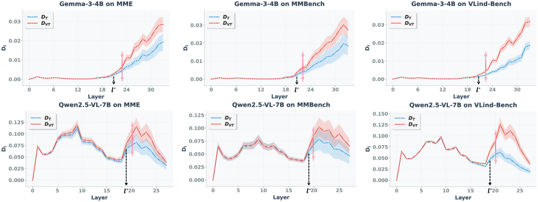
Figure 2: Visual Integration Point. We consistently observe that there is a specific layer $l^{*}$ that clearly distinguish the distance between $Z^{l}_{\text{vis}}$ and $Z^{l}_{\text{blind}}$ across two groups $\mathcal{D}_{\text{VT}}$ and $\mathcal{D}_{\text{T}}$.

In Figure 2, we plot the representation distance estimated for two groups: $\mathcal{D}_{\text{VT}}$ (vision-dependent) in red and $\mathcal{D}_{\text{T}}$ (vision-independent) in blue, across all layers in Qwen2.5-VL-7B (Bai et al., 2025) and Gemma-3-4B (Team et al., 2025). We evaluate on three representative datasets: MME (Yin et al., 2024), MMBench (Liu et al., 2024d), and VLind-Bench (Lee et al., 2025). Since these datasets do not explicitly annotate the degree of visual dependency for each instance ($\mathcal{P}_{\text{VT}}$ vs. $\mathcal{P}_{\text{T}}$), we partition each dataset $\mathcal{D}$ into two auxiliary groups: $\mathcal{D}_{\text{VT}}=\{(x_{v},x_{t})\in\mathcal{D}:F_{\theta}(x_{v},x_{t})\neq F_{\theta}(\varnothing,x_{t})\}$ and $\mathcal{D}_{\text{T}}=\{(x_{v},x_{t})\in\mathcal{D}:F_{\theta}(x_{v},x_{t})=F_{\theta}(\varnothing,x_{t})\}$. This split leverages the prediction agreement between multimodal and text-only inputs as a proxy for task type: if two predictions differ, the sample must have demanded visual information to the model, suggesting membership in $\mathcal{P}_{\text{VT}}$ likely.

From Figure 2, we make four key observations: (1) Existence of VIP. Representation divergence between $\mathcal{D}_{VT}$ and $\mathcal{D}_{T}$ does not show from the beginning. Instead, for both models, we observe a clear visual integration point ($l^{*}$), where the representation distance for the $\mathcal{D}_{\text{VT}}$ group rises more sharply compared to $\mathcal{D}_{\text{T}}$ group, marking the onset of genuine multimodal integration; (2) Behavioral shift across VIP. We observe a notable increase in the standard deviation of representation distances across VIP. Specifically, before VIP, the model exhibits relatively uniform representation distances across samples, suggesting general-purpose information processing. After VIP, the model’s usage of visual information becomes more diverse and instance-dependent to solve a specified task for each query; (3) VIP is dataset-agnostic. Within each model, the location of the VIP is relatively consistent across all datasets. For Qwen2.5-VL-7B, the transition consistently occurs around layers 18–20, and for Gemma-3-4B, the transition is around layers 20–22. This stability suggests that the VIP is primarily the LVLM’s intrinsic property, not one driven by dataset-specific biases; and (4) Model-specific patterns. Despite the shared existence of the VIP, the shape of distance across layers differs across models. In Qwen2.5-VL-7B, representation distance grows relatively smoothly before peaking near the middle-to-late layers and then declines. In contrast, Gemma-3-4B exhibits flat trajectories for many early layers, followed by a steep and monotonic rise after VIP. This suggests that each model has a distinctive hierarchical representation derived from its unique designs.

Overall, these findings highlight not only the universality of the VIP existence, which distinguishes vision-centric decoding (post-$l^{*}$) from general information-gathering behavior (pre-$l^{*}$), but also the variability in how different LVLMs distinctively integrate visual information across depth.

3.3 Quantifying Language Prior of LVLMs through Total Visual Integration

Although the visual integration point detects the birth of $\text{LP}(x,F_{\theta})$, we are also (or even more) interested in how strong $\text{LP}(x,F_{\theta})$ is. To quantify this, we define a total visual integration (TVI) estimator in Def. 3.2, which measures the total amount of visual integration that effectively affects the answer decoding of LVLM, and thus is inversely related to LP in nature.

Definition 3.2 (Total visual integration estimator).

For an observed input $x=(x_{v},x_{t})$, define $x_{\text{vis}}:=(x_{v},x_{t})$ and $x_{\text{blind}}:=(\varnothing,x_{t})$. Given an LVLM $F_{\theta}$ with $L$ decoder layers which produces two sets of chain-of-embedding $(z^{1}_{\text{vis}},...,z^{L}_{\text{vis}})$ and $(z^{1}_{\text{blind}},...,z^{L}_{\text{blind}})$, we define the empirical estimator for the per-sample total visual integration as follows,

$$\text{TVI}(l^{*};x,F_{\theta})=\frac{1}{L-l^{*}+1}\sum_{l=l^{*}}^{L}\big[d(z^{l}_{\text{vis}},z^{l}_{\text{blind}}))\big]\text{,}$$ (4)

where $z^{l}_{\text{vis}}=f_{l}(x_{\text{vis}})$, $z^{l}_{\text{blind}}=f_{l}(x_{\text{blind}})$, and $d(\cdot,\cdot)$ denotes a distance metric.

Here $l^{*}$ marks the VIP layer, where visual information begins to meaningfully influence the model’s internal states. The TVI score then measures the cumulative contribution of visual information by averaging representation distances across all subsequent layers ($l\geq l^{*}$). The idea behind TVI is that once the model passes the visual integration point, its internal representations increasingly reflect meaningful visual grounding, rather than shallow alignment or language-driven statistical patterns. A higher TVI indicates that visual information exerts a stronger and more persistent influence throughout the later layers, while a lower TVI suggests that the model is more likely to remain text-dominated even after $l^{*}$. In this sense, TVI provides a holistic measure of how much the model truly uses vision for actual problem solving: a strong LP corresponds to weak or shallow visual integration (low TVI), while effective multimodal reasoning corresponds to high TVI.

To investigate the distinction between pre-$l^{*}$ and post-$l^{*}$ phases in visual integration, we analyze Spearman’s rank correlation between them and answer correctness on VLind-Bench (Lee et al., 2025), which requires visual reasoning. The results in Table 1 show that correlations are weak and statistically less-significant when TVI is computed over pre-$l^{*}$ layers. In contrast, the post-$l^{*}$ aggregation yields remarkable correlations with the prediction correctness, indicating that only after the VIP, the representation distance becomes strongly associated with task performance, thereby serving as a reliable indicator of effective visual integration. In this paper, we stick with post-$l^{*}$ aggregation in Definition 3.2.

Table 1: Spearman’s rank correlation between prediction correctness and TVI aggregated from different layers.

Model	pre-$l^{*}$	post-$l^{*}$
Qwen2.5-VL-7B	0.1489 ($p=0.002$)	lightblue 0.7241 ($p<0.001$)
Gemma3-4B	0.4659 ($p<0.001$)	lightblue 0.7174 ($p<0.001$)

Taken together, results from Figure 2 and Table 1 highlight two key insights: (1) the existence of the visual integration point $l^{*}$, where effective problem-solving starts to happen by integrating visual information, and (2) the strong relationship between post-$l^{*}$ TVI and downstream performance on vision-dependent tasks. These findings demonstrate that VIP and TVI provide a principled toolkit for analyzing visual integration and language prior in LVLMs. We summarize our findings below.

4 Extended Experiments

Building on the visual integration measurement introduced in the previous section, we conduct additional experiments to assess its empirical validity. Furthermore, we designed a set of in-depth analyses to explore the relationship between visual integration and the language priors in LVLMs.

Figure 3: VIPs of different models observed across different datasets. Our novel framework, fueled by contrasting chain-of-embedding, allows us to consistently observe VIP across multiple models and datasets, and further enables us to estimate TVI to measure language prior.

VIP consistently emerges across different datasets and models.

We extend the experimental setups described in Section 3 to a broader range of 6 datasets and 9 LVLMs, including Qwen2.5-VL-7B (Bai et al., 2025), InternVL3-8B (Zhu et al., 2025), Gemma-3-4B (Team et al., 2025), LLaVA-v1.5-7B (Liu et al., 2024a), Eagle2.5-8B (Chen et al., 2025a), Llama-3.2-11B-Vision, LLaVA-NeXT-Vicuna-7B (Liu et al., 2024b), LLaVA-OV-Qwen2-7B (Li et al., 2025) and SmolVLM (Marafioti et al., 2025). We use the instruction-tuned version for all models. For the dataset, we consider general VQA benchmarks including MME (Chaoyou et al., 2023), MMBench (Liu et al., 2024d), MMStar (Chen et al., 2024), and MMMU (Yue et al., 2024). We also incorporate two benchmarks specifically designed for language prior evaluation, which are VLind-Bench (Lee et al., 2025) and ViLP (Luo et al., 2024). This results in a combination of 54 experimental settings. Implementation details, including data statistics, generation configuration, strategy for VIP selection, etc., are provided in Appendix C. As illustrated in Figure 3, the emergence of VIP is remarkably consistent across all settings: for each model, there exits a clear transition layer $l^{*}$ where the distance between embeddings $Z_{\text{vis}}^{l}$ and $Z_{\text{blind}}^{l}$ increases more significantly for vision-dependent group ($\mathcal{D}_{\text{TV}}$), compared to the vision-independent group ($\mathcal{D}_{\text{T}}$). These results highlight the universality of the VIP existence. The complete experimental results are provided in Appendix D.

TVI reliably differentiates strong vs. weak language prior.

Figure 4: TVI under language priors of different strengths. We see that TVI effectively discerns the differences in strength of LP, thereby standing for a reliable measure for LP.

To examine whether TVI (c.f. Definition 3.2) reliably reflects the strength of the language prior, we contrast results on two complementary datasets: ViLP and MMBench. ViLP is intentionally constructed to induce a strong LP on the data side by designing queries where plausible answers can often be inferred from textual patterns or statistical correlations without the need for visual grounding. In contrast, MMBench represents a weak LP setting, with less misleading questions that elicit more visual grounding. As shown in Figure 4, our analysis reveals that datasets with stronger language priors (e.g., ViLP) yield lower TVI values, indicating weaker visual integration in the model, whereas less biased datasets (e.g., MMBench) produce higher TVI values, reflecting stronger use of visual information. This confirms that TVI serves as a reliable quantitative indicator of LP.

Comparison to existing proxy for language prior.

Table 2: Spearman’s rank correlation between different metrics and answer prediction correctness.

	Qwen2.5-VL-7B		InternVL-3-8B
Metric	VLind	ViLP	VLind	ViLP
lightblue TVI	0.7155 $(p<0.001)$	0.6335 $(p<0.001)$	0.6727 $(p<0.001)$	0.5709 $(p<0.001)$
Visual Attention	0.0871 $(p=0.075)$	-0.0364 $(p=0.530)$	0.4967 $(p<0.001)$	0.0746 $(p=0.197)$
Output Divergence	0.2978 $(p<0.001)$	0.5084 $(p<0.001)$	0.1627 $(p<0.001)$	0.5615 $(p<0.001)$

There are alternative approaches to explain LP proposed in previous works, which rely on output-based or attention-based heuristics by assuming (1) LP manifests as high similarity between output tokens generated with and without visual input (Chen et al., 2025b; Xie et al., 2024), or (2) LP arises due to insufficient attention being allocated to visual tokens (Liu et al., 2025). In Table 2, we compare our TVI with two existing approaches (see Appendix C for detailed formulation), average visual attention and output divergence, by conducting the Spearman’s rank correlation analysis between these measures and the correctness of model predictions on two datasets, which all require integrating visual information to produce correct answers. Our TVI consistently exhibits a stronger correlation with output correctness across all datasets and models, suggesting that TVI stands for a reliable indicator of effective visual integration of LVLMs. In contrast, the other approaches show weak and inconsistent correlations in different scenarios.

We argue that both existing approaches fail to directly capture the true impact of visual integration on the model’s generation. In the case of visual attention, the model may assign high weights to irrelevant regions of the image rather than the areas required for correct reasoning, and ultimately fall back on its language prior to generate the answer—resulting in inflated attention scores but weak correlation with language prior. Meanwhile, solely measuring output-level discrepancy does not fully capture fine-grained behavior exhibited in internal representation dynamics—differences that are more fundamental in nature than what can be observed from final outputs. It shows the significance of procedural aggregation in TVI. We provide additional visualization analysis in Appendix E.

Table 3: Spearman’s rank correlation between correctness and TVI under different distance metrics. Results are based on evaluations using Qwen2.5-VL-7B. All $p$-values are $<0.001$.

Metric	VLind	ViLP
Embedding-based
Cosine Distance	0.7155	0.6335
L2 Distance	0.7123	0.6578
Output-based (w/ logit-lens)
KL Divergence	-0.1693	0.2901
JS Divergence	-0.2261	0.2942

Ablations on distance metrics.

To investigate how different choices of distance metric $d$ affect our ability to capture model behavior, we conduct ablation studies with alternative formulations of TVI. As shown in Table 3, TVI remains a strong indicator of model correctness when computed using the L2 distance between latent embeddings. However, when we apply the logit-lens technique (nostalgebraist, 2020)—projecting hidden states at each layer into the output token space and computing divergence between the resulting distributions—the effectiveness of TVI drops significantly. This degradation suggests that such a projection distorts or suppresses the intermediate behavioral differences that occur during decoding. The output space, shaped by the language modeling head, inherently filters latent representations through a decoding-biased lens, which may obscure subtle but meaningful cross-modal integration patterns. These observations reinforce our central contribution: to faithfully capture the behavioral dynamics of vision-language models, it is essential to examine the internal processing trajectory within the latent representation space, rather than relying on surface-level discrete outputs or their immediate projections. Additional visualization analysis is provided in Appendix E.

Ablations on model scales.

Figure 5: Ablations on model scales. VIP and the dimension-normalized TVI analysis results for three variants of Gemma-3 model family.

We further examine whether our findings generalize across models of different scales. As shown in Figure 5, a clearly defined VIP consistently emerges across models of varying sizes (4B, 12B, and 27B), underscoring the robustness and generality of our proposed behavioral analysis framework. Interestingly, we also find that the VIP tends to appear at a similar relative depth, which is approximately 60% of the total number of layers, regardless of model size. In addition, after normalizing by the dimensionality of hidden states, we observe that the average normalized TVI is consistently higher in larger models on both $\mathcal{D}_{\text{VT}}$ and $\mathcal{D}_{\text{T}}$. This suggests that larger models are more effective at leveraging visual information in a uniform manner across diverse input types, thereby exhibiting greater robustness to misleading language priors. These observations collectively reinforce the broader applicability of our framework in analyzing visual integration behavior across model scales.

5 Theoretical Analysis

We provide a new interpretation for our metric, $\mathbf{D}_{l}(\mathcal{P}_{\text{VT}},F_{\theta})-\mathbf{D}_{l}(\mathcal{P}_{\text{T}},F_{\theta})$, that locates VIP (Theorem 5.1) and how we can practically employ the expected representation distance (Theorem 5.2) through theoretical analyses. All the proofs and an additional theorem that justifies the use of our empirical representation distance (Lemma F.1) are given in Appendix F.

Information-theoretic interpretation on representation divergence.

By recasting the representation distance measurement as a density estimation problem, i.e., $d(Z^{l}_{\text{vis}},Z^{l}_{\text{blind}})\propto-\log\hat{p}_{\text{T}}(Z^{l})$ (please see Lemma F.2), we show that the difference in expected representation distances, $\mathbf{D}_{l}(\mathcal{P}_{\text{VT}},F_{\theta})-\mathbf{D}_{l}(\mathcal{P}_{\text{T}},F_{\theta})$, which we call representation divergence here, can be interpreted as a relative distributional discrepancy that measures how far our density estimator $\hat{p}_{\text{T}}(Z^{l})$, defined by $d(Z^{l}_{\text{vis}},Z^{l}_{\text{blind}})$, from a population distribution $p_{\text{VT}}(Z^{l})$ compared to $p_{\text{T}}(Z^{l})$ in Theorem 5.1.

Theorem 5.1.

Let $X=(X_{v},X_{t})\in\mathcal{X}$ be a random variable from $\mathcal{P}_{\text{VT}}$ or $\mathcal{P}_{\text{T}}$, and $f_{l}:\mathcal{X}\rightarrow\mathcal{Z}$ be a layer stack from an LVLM $F_{\theta}$. For $\mathcal{P}_{\text{T}}$, define a density estimator $\hat{p}_{\text{T}}(Z^{l}):=\mathcal{N}(f_{l}(X_{t}),I)$, and denote $p_{\text{VT}}(Z^{l})$ (resp. $p_{\text{T}}(Z^{l})$) as the population distribution on $Z^{l}=f_{l}(X)$ derived from $\mathcal{P}_{\text{VT}}$ (resp. $\mathcal{P}_{\text{T}}$). Then, given $d(Z_{1},Z_{2}):=\frac{1}{2}||Z_{1}-Z_{2}||_{2}^{2}$, the difference in the expected representation distances between $\mathcal{P}_{\text{VT}}$ and $\mathcal{P}_{\text{T}}$, i.e., $\mathbf{D}_{l}(\mathcal{P}_{\text{VT}},F_{\theta})-\mathbf{D}_{l}(\mathcal{P}_{\text{T}},F_{\theta})$, can be expressed as follows,

$$\text{KL}\big(p_{\text{VT}}(Z^{l})||\hat{p}_{\text{T}}(Z^{l})\big)-\text{KL}\big(p_{\text{T}}(Z^{l})||\hat{p}_{\text{T}}(Z^{l})\big)+\bar{\mathbf{H}},$$ (5)

where $\bar{\mathbf{H}}$ is a constant $H\big(p_{\text{VT}}(Z^{l})\big)-H\big(p_{\text{T}}(Z^{l})\big)$, and $\text{KL}(\cdot||\cdot)$ denotes the KL divergence.

Analytic bounds on representation divergence for practical use.

We have assumed a fixed model $F_{\theta}$ so far. If one is willing to adapt the model to improve its effective visual integration, the analytic bounds in Theorem 5.2 described with $\mathcal{H}$-divergence (see Def. F.4) can be useful.

Theorem 5.2.

Let $X=(X_{v},X_{t})\in\mathcal{X}$ be a random variable of a multimodal input query. Given a stack of LVLM layers $f_{l}:\mathcal{X}\rightarrow\mathcal{Z}$ and a distance metric $d:\mathcal{Z}\times\mathcal{Z}\rightarrow[0,1]$, define a hypothesis $h=d(f_{l}(X_{v},X_{t}),f_{l}(X_{t})):\mathcal{X}\rightarrow[0,1]$ and a set of these hypotheses $\mathcal{H}$ that has a pseudo-dimension $c$. Then, for $\mathbf{D}_{l}(\mathcal{P}_{\star},F_{\theta}):=\mathbb{E}_{X\sim\mathcal{P}_{\star}}[h(X)]$ with any $\mathcal{P}_{\text{VT}}$, $\mathcal{P}_{\text{T}}$, and $\mathcal{P}_{\text{M}}:=\frac{\mathcal{P}_{\text{VT}}+\mathcal{P}_{\text{T}}}{2}$, and the empirical distributions $\mathcal{D}_{\text{VT}}\sim\mathcal{P}_{\text{VT}}$ and $\mathcal{D}_{\text{T}}\sim\mathcal{P}_{\text{T}}$ of $N$ samples for each, we have the following bounds w.p. at least $1-\delta$ for $0<\delta<1$,

$$\text{i})\ \ 1-\mathbf{D}_{l}(\mathcal{D}_{\text{T}},F_{\theta})-\frac{1}{2}d_{\bar{\mathcal{H}}}(\mathcal{D}_{\text{VT}},\mathcal{D}_{\text{T}})-\tilde{\mathcal{O}}_{\delta}\leq\mathbf{D}_{l}(\mathcal{P}_{\text{VT}},F_{\theta}),$$ (6)

$$\text{ii})\ \ \frac{1}{2}-\frac{1}{4}d_{\bar{\mathcal{H}}}(\mathcal{D}_{\text{VT}},\mathcal{D}_{\text{T}})-\tilde{\mathcal{O}}_{\delta}\leq\mathbf{D}_{l}(\mathcal{P}_{\text{M}},F_{\theta})\leq\frac{1}{2}+\frac{1}{4}d_{\bar{\mathcal{H}}}(\mathcal{D}_{\text{VT}},\mathcal{D}_{\text{T}})+\tilde{\mathcal{O}}_{\delta}$$ (7)

where $\bar{\mathcal{H}}:=\{\mathbb{I}_{|h(X)-h^{\prime}(X)|>t}:h,h^{\prime}\in\mathcal{H},0\leq t\leq 1\}$ and $\tilde{\mathcal{O}}_{\delta}:=\mathcal{O}(\sqrt{\frac{1}{N}(\log\frac{1}{\delta}+c\log\frac{N}{c})})$.

6 Conclusion

In this work, we present a formal framework for understanding and quantifying the language prior in LVLMs by contrasting the chain-of-embedding between visual and blind contexts. Through this framework, we identify the consistent existence of the Visual Integration Point (VIP), a specific layer at which the model begins to meaningfully incorporate visual context for task-solving beyond the shallow information gathering. Building on this observation, we propose a new metric named Total Visual Integration (TVI), which estimates the degree of effective visual integration and therefore language prior. We conduct comprehensive experiments across 9 LVLMs and 6 datasets, and the results demonstrate that our framework robustly works across models and tasks, providing consistent and interpretable signals about the presence and strength of language prior. Finally, we present some theorems for better understanding and justification of our framework. We hope that this work sheds light on the internal mechanisms of multimodal models and provides a foundation for diagnosing the language prior, ultimately guiding the development of reliable and responsible LVLMs.

Ethics Statement

This work conducts empirical and analytical studies on the internal behavior of LVLMs, with the goal of understanding and quantifying their reliance on language priors and the extent of visual information integration during inference. To pursue high standards of scientific excellence, we propose a formal framework with clear definitions of all used terms and conduct validation at scale, e.g., 54 combinations of models and datasets, and we further provide theoretical analyses on our framework. Our study does not involve any human subjects, personally identifiable information, or sensitive data. All experiments are conducted using publicly available models and benchmark datasets that are widely adopted in the multimodal learning community. Our proposed metrics and analyses are intended for research and diagnostic purposes. By providing tools to diagnose when LVLMs rely on text versus vision, we aim to support more accountable model development and contribute positively to the responsible advancement of AI. We encourage future work to further validate these findings under more diverse real-world conditions.

Reproducibility Statement

All of the models and datasets we used in this work are publicly available. To further ensure the reproducibility of our findings, we provide comprehensive descriptions of all experimental settings, including dataset preprocessing, model configurations, metric definitions, and evaluation protocols, in Section 4 and Appendix C. Our framework does not require model re-training or fine-tuning, and all evaluations are conducted in a zero-shot setting using publicly available model checkpoints, which minimizes computational and hardware requirements. We release the complete codebase for our analysis framework, including tools for data preparation, TVI computation, and visualization, at the following repository: .

Appendix

Contents

Figure 6: Complete experimental results. (Part 1)

Figure 7: Complete experimental results. (Part 2)

Figure 8: Complete experimental results. (Part 3)

Appendix A Related Work

Visual perception in LVLMs.

Most mainstream LVLMs (Liu et al., 2023; 2024a; 2024b; Bai et al., 2025; Dai et al., 2023) adopt a late-fusion architecture comprising three key components: a vision backbone, a language model that processes both image and text tokens, and a modality adapter that aligns visual representations with the language space. The visual understanding capabilities of these models largely depend on the perception quality of pre-trained vision encoders (e.g., CLIP (Radford et al., 2021), SigLIP (Zhai et al., 2023)) and the reasoning ability of large-scale language models.

Despite promising results on some multimodal benchmarks, this paradigm has been recently challenged due to its poor performance on vision-centric tasks, suggesting that these models often fail to truly see the image (Tong et al., 2024b; a; Vo et al., 2025). A growing body of work has sought to uncover how visual perception operates internally within LVLMs. For example, Bi et al. (2025); Jiang et al. (2025); Neo et al. (2025) examine the layer-wise attention patterns and identify distinct phases of visual integration, typically emerging in the mid-to-late layers. Venhoff et al. (2025) utilize pre-trained sparse autoencoders (SAEs) as analytical tools to show that visual representations gradually align with language representations over depth, converging in the later layers. Complementarily, Fu et al. (2025) apply probing techniques and argue that language decoders in existing LVLMs struggle to effectively leverage the visual features produced by their vision backbones. Their findings suggest that the bottleneck lies not in the availability of visual information but in feature misalignment.

Language prior in LVLMs.

One of the most prominent limitations of current LVLMs is their tendency to overly rely on language priors, often generating plausible outputs without grounding in the visual context. This behavior—commonly referred to as the language prior problem—has drawn increasing attention. Recent studies attempt to evaluate this phenomenon by designing datasets that stress-test visual grounding. For example, Lee et al. (2025) and Luo et al. (2025) construct datasets with counterfactual visual inputs to assess whether models can disentangle visual signals from misleading linguistic cues. Similarly, Deng et al. (2025) test modality conflict scenarios to evaluate the model’s preference between text and image inputs.

While these works help reveal the presence of language priors, they offer limited insight into the underlying causes. Most current understandings of language prior are based on two widely adopted assumptions: (1) it manifests as high similarity between outputs with and without visual input (Chen et al., 2025b; Xie et al., 2024), and (2) it arises due to insufficient attention allocated to visual tokens (Liu et al., 2025). Building on these assumptions, several works propose methods to mitigate language priors—such as contrastive decoding (Favero et al., 2024) or inference-time attention reallocation (Liu et al., 2024c). Others, like Chen et al. (2025b) and Xie et al. (2024), explore training-time interventions that penalize outputs overly aligned with the model’s default language predictions.

Appendix B Discussion on Visual Integration Point

B.1 Configuration and Practice

In Eq. 8, we chracterized the VIP $l^{*}$ based on the pre-$l^{*}$ and post-$l^{*}$ representation divergences $\mathbf{D}_{l}(\mathcal{P}_{\text{VT}},F_{\theta})-\mathbf{D}_{l}(\mathcal{P}_{\text{T}},F_{\theta})$ where the pre-$l^{*}$ chain-of-embeddings shows nearly zero representation divergence whereas the post-$l^{*}$ chain-of-embeddings exhibits an effectively large representation divergence defined by positive $\tau$. In practice, we can not access the population distribution $\mathcal{P}_{\text{VT}}$ and $\mathcal{P}_{\text{T}}$, therefore we can not compute the truth expected representation distance $\mathbf{D}_{l}(\mathcal{P}_{\star},F_{\theta})$. What we do in practice is estimate that expected representation distance with finite samples $\mathcal{D}_{\text{VT}}$ and $\mathcal{D}_{\text{T}}$. We observed that this empirical estimator (Eq. 2) is actually well aligned with our hypothesis, yet there can be some cases where the fitness of the estimator is bad, e.g., Figure 9. However, even in that case, the point $l^{*}$, where the empirical representation divergence exceeds a positive constant for all subsequent layers, consistently emerges, and the TVI (Eq. 4) is calculated based on that $l^{*}$ becomes a strong indicator of LP.

B.2 Algorithmic Estimation on Visual Integration Point

As discussed in §3.2, identifying the VIP provides valuable insights into when visual information begins to influence answer decoding. In most cases, we rely on empirical observation of the representation distance curves to determine $l^{*}$, which proves to be straightforward and interpretable across a wide range of models. However, in situations where manual inspection is impractical — e.g., for large-scale model comparisons or automated pipelines — it may be desirable to estimate the VIP programmatically. To this end, we introduce an optional empirical estimator that can automatically approximate the VIP given a model and a dataset. While not required for our core analysis, this estimation method serves as a practical tool in settings where manual identification of $l^{*}$ is infeasible.

Definition B.1 (Visual integration point estimator).

For a dataset $\mathcal{D}$ sampled from a mixture distribution $\mathcal{P}=(1-\lambda)\mathcal{P}_{\text{VT}}+\lambda\mathcal{P}_{\text{T}}$ for $\lambda\in(0,1)$ and an LVLM $F_{\theta}$ with $L$ decoder layers which produces a chain-of-embedding $(Z^{1},...,Z^{L})$ given input, let $\mathcal{L}$ be the index set of LVLM decoder layers and $\mathbf{D}_{l}$ be an expected representation distance defined as Eq. 2. An empirical visual integration point estimator is as follows,

$$\text{VIP}(\mathcal{D},F_{\theta}) =\arg\min_{l\in\mathcal{L}\backslash L}\big[\mathbf{D}_{l}(\mathcal{D}_{\text{VT}},F_{\theta})-\mathbf{D}_{l}(\mathcal{D}_{\text{T}},F_{\theta})\geq\alpha\cdot\frac{\sigma_{l}}{\mathbf{D}_{l}(\mathcal{D},f)}\big],$$ (8)

where $\alpha$ is a pre-defined coefficient and $\sigma_{l}$ denotes the sample standard deviation of the observed representation distance over $\mathcal{D}$.

$\text{VIP}(\mathcal{D},F_{\theta})$ can be interpreted as the layer index where the average $d(\cdot,\cdot)$ on $\mathcal{D}_{\text{VT}}$ first exceeds that on $\mathcal{D}_{\text{T}}$ up to an empirical coefficient of variation (Everitt & Skrondal, 2010) of $d(\cdot,\cdot)$ on $l$-th layer. Besides, one can also devise another VIP estimator based on the test statistic we discuss in Eq 10 of Lemma F.1 by specifying arbitrary significance levels that the user prefers.

Appendix C Implementation Details

Models.

We evaluate our framework on 9 publicly available LVLMs, covering a diverse range of architectures and training paradigms. For all models, we use the official instruction-tuned checkpoints available on Hugging Face. To ensure consistent comparison across models, we set the generation temperature to 0.

Datasets.

Our evaluation spans 6 benchmark datasets, each consisting of either binary (‘Yes/No’) or multiple-choice questions. This design ensures that the hidden state of the final token—used for representation distance calculations—is closely tied to the model’s reasoning process. For MMMU, we use the validation set and filter out samples that involve more than one image or open-ended output to ensure consistency in the evaluation setting. Also, when constructing the prompt, we do not use the provided explanations for fair comparison. For ViLP, we consistently select image3 and answer3 to curate our (counterfactual) VQA pair. For VLind-Bench, we convert each annotated counterfactual statement into a binary ‘Yes/No’ question. To perform this transformation, we use the advanced language model GPT-4o with the following prompt:

Figure 9: Experimental results under controlled settings. We use a synthetic baseline constructed from CommonsenseQA questions paired with irrelevant images as $\mathcal{D}_{\text{T}}$ (vision-independent), while standard VQA benchmarks (MME, MMBench, and VLind-Bench) are used as $\mathcal{D}_{\text{VT}}$ (vision-dependent).

The models are instructed to directly generate the answer under a zero-shot setting, without involving any reasoning steps. Additional statistics of each dataset and corresponding splits are provided in Table 4.

To further validate the reliability of the agreement-based separation introduced in §3.2, and to demonstrate that our analysis can generalize to scenarios with known visual dependencies, we construct a controlled baseline dataset. Specifically, we take questions from CommonsenseQA (Talmor et al., 2018), which are inherently language-only, and pair each question with a randomly selected, irrelevant image from COCO 2017-val (Lin et al., 2014), forming a synthetic VQA setting that does not require visual input. We treat this as our vision-independent group $\mathcal{D}_{T}$. For the vision-dependent group $\mathcal{D}_{VT}$, we use samples from standard VQA benchmarks such as MME, MMBench, and VLind-Bench, which typically require more grounding in visual content. As shown in Figure 9, the average TVI is significantly lower for the baseline $\mathcal{D}_{T}$ compared to the general VQA datasets, confirming that the model does not extract meaningful information from irrelevant visual input. In contrast, even in the presence of strong language priors, the model still benefits from image content in $\mathcal{D}_{VT}$. It is also worth noting that there is a reverse trend before VIP for Qwen2.5-VL-7B, indicating representation distance before VIP is not associated with the actual meaningful visual integration during decoding. These findings are consistent with our previous results and further support the effectiveness of our proposed separation framework. Nonetheless, to ensure better control over data attributes such as format and context length, and to reveal clearer trends, we continue to use the agreement-based separation strategy in the main text.

Table 4: Dataset statistics. M stands for multiple-choice and B stands for binary-choice (Yes/No). Qwen2.5-VL-7B is used as an example here.

Statistics	MME	MMBench	MMStar	MMMU	VLind-Bench	ViLP
Question Type	B	M	M	M	B	M
$|\mathcal{D}|$	2374	4377	1500	805	418	300
$|\mathcal{D}_{VT}|$	546	2782	1057	446	144	177
$|\mathcal{D}_{T}|$	1828	1595	443	359	274	123

Metrics.

All TVI values reported in our experiments are computed based on empirically determined Visual Integration Points (VIPs) specific to each model. The following VIPs are used: Qwen2.5-VL-7B (18), InternVL3-8B (16), Gemma-3-4B (20), Gemma-3-12B (26), Gemma-3-27B (35), LLaVA-v1.5-7B (9), Eagle2.5-8B (15), Llama-3.2-11B-Vision (12), LLaVA-NeXT-Vicuna-7B (12), LLaVA-OV-Qwen2-7B (15) and SmolVLM (15). We also provide an automatic method for estimating VIP in Appendix B.2 for potential practical usage. Representation distances are computed using the hidden states corresponding to the last generated token. The metrics introduced in §4 are computed as follows:

$$\text{Visual Attention}=\frac{1}{LH}\sum_{l=1}^{L}\sum_{h=1}^{H}\alpha^{(l,h)},\quad\text{Output Divergence}=d(Z^{L}_{\text{vis}},Z^{L}_{\text{blind}})$$ (9)

where $\alpha^{(l,h)}$ denotes the total attention from the final generated token to all preceding visual tokens in head $h$ at layer $l$, and $Z^{L}$ represents the hidden state at the final layer.

Appendix D Additional Experimental Results

We provide the complete experimental results on 9 LVLMs and 6 datasets in Figure 6, 7, 8. Across all models and datasets, a consistent existence of the VIP can be observed. However, for some models, such as SmolVLM, the divergence between $\mathcal{D}_{VT}$ and $\mathcal{D}_{T}$ is less pronounced, likely due to the model’s limited capacity and thus less promising visual integration.

Appendix E Further Analysis

In this section, we elaborate on the limitations of attention-based and output-based analysis for language prior in LVLMs.

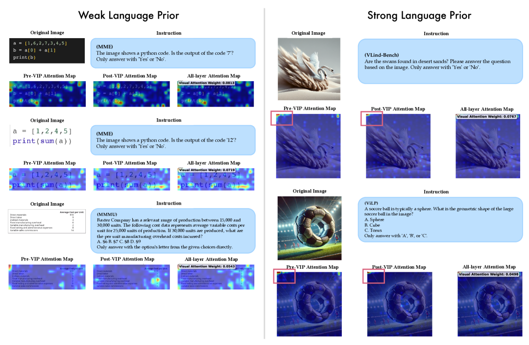
Figure 10: Visualization of visual attention maps under weak and strong language priors.

First, for attention-based methods, we argue that a higher visual attention weight does not necessarily imply better visual grounding. As shown in Figure 10, under weak language priors, the model is able to correctly attend to the key areas that are semantically related to the given instruction. However, under strong language priors, we observe a pathological attention pattern in which the model’s attention becomes abnormally concentrated in a limited region of the image. We refer to this phenomenon as an attention sink. In such cases, although the aggregated visual attention weight appears high, it does not reflect meaningful visual processing. Instead, the model is effectively bypassing genuine visual understanding by fixating on irrelevant or static regions, thereby undermining the utility of attention-based metrics as reliable indicators of visual integration.

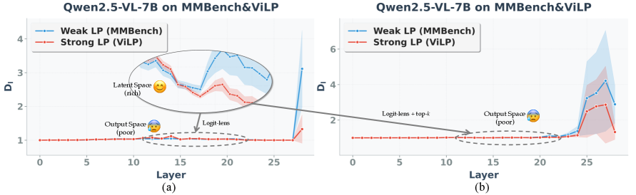
Figure 11: Layer-wise representation distances in latent space vs. output space. We apply the logit-lens to project hidden states at each layer into the output space. In (a), distances are computed over the entire output vector, while in (b), they are restricted to the top-$k$ token positions corresponding to candidate answer options.

To better understand why output-based representations are less effective in capturing language prior behavior, we visualize how representation distances vary across the latent and output spaces. As shown in Figure 11, the projection from the latent space to the output token space tends to obscure semantic distinctions that are otherwise indicative of the model’s underlying behavior—such as whether it is performing effective visual grounding or defaulting to language priors. This observation aligns with our earlier argument: surface-level outputs alone may not faithfully reflect the internal decision-making process of LVLMs. Instead, meaningful behavioral signals often reside in the deeper latent representations, emphasizing the importance of analyzing internal dynamics rather than relying solely on output-level comparisons.

Appendix F Details on Theoretical Analysis and Proofs

F.1 Justification and Interpretation on Representation Divergence

We first show that our empirical estimate for the difference in the expected representation distances (Eq. 3) can be viewed as a two-sample test statistic with asymptotic normality in Lemma F.1.

Lemma F.1.

Let $X=(X_{v},X_{t})\in\mathcal{X}$ be a random variable sampled from $\mathcal{P}_{\text{VT}}$ or $\mathcal{P}_{\text{T}}$, and denote $\mathcal{D}_{\text{VT}}\sim\mathcal{P}_{\text{VT}}$ and $\mathcal{D}_{\text{T}}\sim\mathcal{P}_{\text{T}}$ as empirical distributions with $N$ and $M$ i.i.d. samples, respectively. Given a stack of LVLM layers $f_{l}:\mathcal{X}\rightarrow\mathcal{Z}$ from $F_{\theta}$ and a distance metric $d:\mathcal{Z}\times\mathcal{Z}\rightarrow\mathbb{R}$ with a finite second moment, the difference in the expected representation distance estimates $\mathbf{D}_{l}(\cdot,\cdot)$ between $\mathcal{D}_{\text{VT}}$ and $\mathcal{D}_{\text{T}}$ is a two-sample test statistic with asymptotic normality, that is,

$$\mathbf{D}_{l}(\mathcal{D}_{\text{TV}},F_{\theta})-\mathbf{D}_{l}(\mathcal{D}_{\text{T}},F_{\theta})\overset{\underset{\mathrm{approx}}{}}{\sim}\mathcal{N}(\mu_{\text{T}}-\mu_{\text{VT}},\frac{\sigma^{2}_{\text{T}}}{M}+\frac{\sigma^{2}_{\text{VT}}}{N})\quad\text{as}\;\;N,M\rightarrow\infty,$$ (10)

where $\mu_{\text{VT}}=\mathbf{D}_{l}(\mathcal{P}_{\text{VT}},F_{\theta})$, $\mu_{\text{T}}=\mathbf{D}_{l}(\mathcal{P}_{\text{T}},F_{\theta})$ and $\sigma^{2}_{\text{VT}}=\text{Var}_{\mathcal{P}_{\text{VT}}}[d(f_{l}(X_{v},X_{t}),f_{l}(X_{t}))]<\infty$, $\sigma^{2}_{\text{T}}=\text{Var}_{\mathcal{P}_{\text{T}}}[d(f_{l}(X_{v},X_{t}),f_{l}(X_{t}))]<\infty$.

Proof.

Let $\mathcal{I}_{\text{VT}}$ and $\mathcal{J}_{\text{T}}$ be the index sets of $N$ and $M$ i.i.d. samples from $\mathcal{P}_{\text{VT}}$ and $\mathcal{P}_{\text{T}}$, respectively. If samples from $\mathcal{P}_{\text{VT}}$ and $\mathcal{P}_{\text{T}}$ are independent, with finite second moments, we have,

$$\mathbf{D}_{l}(\mathcal{D}_{\text{VT}},F_{\theta})-\mathbf{D}_{l}(\mathcal{D}_{\text{T}},F_{\theta})$$ (11)

$$=\frac{\sum_{i\in\mathcal{I}_{\text{VT}}}[d(f_{l}(x^{i}_{v},x^{i}_{t}),f_{l}(x^{i}_{t}))]}{N}-\frac{\sum_{j\in\mathcal{J}_{\text{T}}}[d(f_{l}(x^{j}_{v},x^{j}_{t}),f_{l}(x^{j}_{t}))]}{M}$$ (12)

$$\sim\mathcal{N}(\mu_{\text{T}}-\mu_{\text{VT}},\frac{\sigma^{2}_{\text{T}}}{M}+\frac{\sigma^{2}_{\text{VT}}}{N}) N,M\rightarrow\infty$$ (by Central Limit Theorem as )

Note that, even though the samples from $\mathcal{P}_{\text{VT}}$ and $\mathcal{P}_{\text{T}}$ are not independent, the asymptotic normality still holds by considering covariance terms between the two distributions. ∎

Now, in Lemma F.2, we provide a new interpretation of our representation distance measure between CoE by casting the distance measurement as a density estimation problem.

Lemma F.2.

Let $X=(X_{v},X_{t})\in\mathcal{X}$ be a random variable sampled from $\mathcal{P}_{\text{VT}}$ or $\mathcal{P}_{\text{T}}$, and $f_{l}:\mathcal{X}\rightarrow\mathcal{Z}$ be a stack of LVLM layers. For $\mathcal{P}_{\text{T}}$, define a density estimator $\hat{p}_{\text{T}}(Z^{l}):=\mathcal{N}(f_{l}(X_{t}),I)$. Given a squared $l_{2}$ distance $d(Z_{1},Z_{2}):=\frac{1}{2}||Z_{1}-Z_{2}||_{2}^{2}$, the representation distance $d(f_{l}(X_{v},X_{t}),f_{l}(X_{t}))$ is the negative log-likelihood estimate of $Z^{l}$ from $\mathcal{P}_{\text{T}}$, denoted as $\hat{p}_{\text{T}}(Z^{l})$, up to an additive constant, and is a strictly proper scoring rule. That is,

$$d(f_{l}(X_{v},X_{t}),f_{l}(X_{t}))\triangleq-\log\hat{p}_{\text{T}}(Z^{l})+\log C,$$ (13)

where $C=(2\pi)^{-\frac{d_{z}}{2}}$ is a normalizing constant for the $d_{z}$-dimensional unit-variance Gaussian.

Proof.

It is easy to check,

$$\hat{p}_{\text{T}}(Z^{l}) =\mathcal{N}(Z^{l}_{\text{blind}},I)$$ (14)

$$\hat{p}_{\text{T}}(Z^{l}) =C\cdot\exp(-\frac{||Z^{l}-Z^{l}_{\text{blind}})||_{2}^{2}}{2})$$ (15)

$$\log\hat{p}_{\text{T}}(Z^{l}) =\log C-\frac{||Z^{l}-Z^{l}_{\text{blind}}||_{2}^{2}}{2}$$ (16)

$$\log\hat{p}_{\text{T}}(Z^{l}) =\log C-d(Z^{l},Z^{l}_{\text{blind}})$$ (17)

where $Z_{\text{blind}}=f_{l}(X_{t})$. In addition, the logarithm of the likelihood is a strictly proper scoring rule (Gneiting & Raftery, 2007), and an offset translation of it is also a strictly proper scoring. ∎

On top of this new framing, i.e., distance measurement as a density estimation problem, we further provide an information-theoretic interpretation of the difference in expected representation distance in Theorem F.3.

Theorem F.3 (Restatement of Theorem 5.1).

Let $X=(X_{v},X_{t})\in\mathcal{X}$ be a random variable from $\mathcal{P}_{\text{VT}}$ or $\mathcal{P}_{\text{T}}$, and $f_{l}:\mathcal{X}\rightarrow\mathcal{Z}$ be a layer stack from an LVLM $F_{\theta}$. For $\mathcal{P}_{\text{T}}$, define a density estimator $\hat{p}_{\text{T}}(Z^{l}):=\mathcal{N}(f_{l}(X_{t}),I)$, and denote $p_{\text{VT}}(Z^{l})$ (resp. $p_{\text{T}}(Z^{l})$) as the population distribution on $Z^{l}=f_{l}(X)$ derived from $\mathcal{P}_{\text{VT}}$ (resp. $\mathcal{P}_{\text{T}}$). Then, given $d(Z_{1},Z_{2}):=\frac{1}{2}||Z_{1}-Z_{2}||_{2}^{2}$, the difference in the expected representation distances between $\mathcal{P}_{\text{VT}}$ and $\mathcal{P}_{\text{T}}$, i.e., $\mathbf{D}_{l}(\mathcal{P}_{\text{VT}},F_{\theta})-\mathbf{D}_{l}(\mathcal{P}_{\text{T}},F_{\theta})$, can be expressed as follows,

$$\text{KL}\big(p_{\text{VT}}(Z^{l})||\hat{p}_{\text{T}}(Z^{l})\big)-\text{KL}\big(p_{\text{T}}(Z^{l})||\hat{p}_{\text{T}}(Z^{l})\big)+\bar{\mathbf{H}},$$ (18)

where $\bar{\mathbf{H}}$ is a constant $H\big(p_{\text{VT}}(Z^{l})\big)-H\big(p_{\text{T}}(Z^{l})\big)$, and $\text{KL}(\cdot||\cdot)$ denotes the KL divergence.

Proof.

$$\mathbf{D}_{l}(\mathcal{P}_{\text{VT}},F_{\theta})-\mathbf{D}_{l}(\mathcal{P}_{\text{T}},F_{\theta})$$

$$=\mathbb{E}_{\mathcal{P}_{\text{VT}}}[d(f_{l}(X_{v},X_{t}),f_{l}(X_{t}))]-\mathbb{E}_{\mathcal{P}_{\text{T}}}[d(f_{l}(X_{v},X_{t}),f_{l}(X_{t}))]$$ (19)

$$=\mathbb{E}_{p_{\text{VT}}(Z^{l})}[-\log\hat{p}_{\text{T}}(Z^{l})+\log C]-\mathbb{E}_{p_{\text{T}}(Z^{l})}[-\log\hat{p}_{\text{T}}(Z^{l})+\log C]$$ (20)

$$=\mathbb{E}_{p_{\text{VT}}(Z^{l})}[-\log\hat{p}_{\text{T}}(Z^{l})]-\mathbb{E}_{p_{\text{T}}(Z^{l})}[-\log\hat{p}_{\text{T}}(Z^{l})]$$ (21)

$$=H\big(p_{\text{VT}}(Z^{l}),\hat{p}_{\text{T}}(Z^{l})\big)-H\big(p_{\text{T}}(Z^{l}),\hat{p}_{\text{T}}(Z^{l})\big)$$ (22)

$$=\big[\text{KL}\big(p_{\text{VT}}(Z^{l})||\hat{p}_{\text{T}}(Z^{l})\big)+H\big(p_{\text{VT}}(Z^{l})\big)\big]-\big[\text{KL}\big(p_{\text{T}}(Z^{l})||\hat{p}_{\text{T}}(Z^{l})]\big)+H\big(p_{\text{T}}(Z^{l})\big)\big]$$ (23)

where $H(\cdot)$ and $H(\cdot,\cdot)$ denote entropy and cross-entropy, respectively. Here, Eq. 20 holds by Lemma F.2, and the remaining equality is trivial by the definitions of $d()$ and information theoretic measures. ∎

F.2 Notations and Problem Setup for Theorem F.6

We recast the problem of measuring the representation distance $d(Z_{\text{vis}},Z_{\text{blind}})$ as a binary classification task, where we want to classify the sample $(Z_{\text{vis}},Z_{\text{blind}})$ into 1 if it originates from the distribution $\mathcal{P}_{\text{VT}}$ while 0 for the samples from $\mathcal{P}_{\text{T}}$.

To be specific, let $\mathcal{X}$, $\mathcal{Z}$, and $\mathcal{Y}$ denote input, LVLM representation, and output, respectively. We have a multimodal input query $X=(X_{v},X_{t})\in\mathcal{X}$, a stack of LVLM layers $f_{l}:\mathcal{X}\rightarrow\mathcal{Z}$, and a distance metric $d:\mathcal{Z}\times\mathcal{Z}\rightarrow[0,1]$. With that, we define a hypothesis $h=d(f_{l}(X_{v},X_{t}),f_{l}(X_{t})):\mathcal{X}\rightarrow[0,1]$ as a real value function to measure the relative likelihood that the input $X$ is sampled from $\mathcal{P}_{\text{VT}}$ rather than $\mathcal{P}_{\text{T}}$, and we also define the labeling function $h^{\star}:\mathcal{X}\rightarrow\{0,1\}$ that maps the input into its ground-truth membership, i.e., 1 if it’s from $\mathcal{P}_{\text{VT}}$ and 0 if it’s from $\mathcal{P}_{\text{T}}$. Then, we formulate an expected error (a.k.a. risk) of a hypothesis $h$ w.r.t. the labeling function $h^{\star}$ on a distribution $\mathcal{P}$ as follows: $\varepsilon_{\mathcal{P}}(h,h^{\star}):=\mathbb{E}_{X\sim\mathcal{P}}[|h(X)-h^{\star}(X)|]$.

Besides, in Def. F.4, we introduce a measure of discrepancy between two distributions, $\mathcal{H}$-divergence, which has been widely adopted in domain adaptation literature (Ben-David et al., 2006; 2010; Ganin et al., 2016; Zhao et al., 2018).

Definition F.4 ($\mathcal{H}$-divergence, (Ben-David et al., 2006; 2010)).

Let $\mathcal{P}$ and $\mathcal{P}^{\prime}$ be probability distributions on the input domain $\mathcal{X}$, and $\mathcal{H}$ be a hypothesis class for $\mathcal{X}$. Denote $\mathcal{A}_{\mathcal{H}}:=\{h^{-1}(1)|h\in\mathcal{H}\}$ as a collection of subsets of $\mathcal{X}$ that are the support of some hypotheses in $\mathcal{H}$. Then, the distance between $\mathcal{P}$ and $\mathcal{P}^{\prime}$ based on $\mathcal{H}$ is defined as follows:

$$d_{\mathcal{H}}(\mathcal{P},\mathcal{P}^{\prime})=2\;\sup_{A\in\mathcal{A}_{\mathcal{H}}}|\mathbb{P}_{\mathcal{P}}[A]-\mathbb{P}_{\mathcal{P}^{\prime}}[A]|.$$ (24)

Now, we are ready to present the proof for Proposition 5.2 in the next subsection.

F.3 Proof for Theorem F.6

Theorem F.5 (Restatement of Theorem 5.2).

Let $X=(X_{v},X_{t})\in\mathcal{X}$ be a random variable of a multimodal input query. Given a stack of LVLM layers $f_{l}:\mathcal{X}\rightarrow\mathcal{Z}$ and a distance metric $d:\mathcal{Z}\times\mathcal{Z}\rightarrow[0,1]$, define a hypothesis $h=d(f_{l}(X_{v},X_{t}),f_{l}(X_{t})):\mathcal{X}\rightarrow[0,1]$ and a set of these hypotheses $\mathcal{H}$ that has a pseudo-dimension $c$. Then, for $\mathbf{D}_{l}(\mathcal{P}_{\star},F_{\theta}):=\mathbb{E}_{X\sim\mathcal{P}_{\star}}[h(X)]$ with any $\mathcal{P}_{\text{VT}}$, $\mathcal{P}_{\text{T}}$, and $\mathcal{P}_{\text{M}}:=\frac{\mathcal{P}_{\text{VT}}+\mathcal{P}_{\text{T}}}{2}$, and the empirical distributions $\mathcal{D}_{\text{VT}}\sim\mathcal{P}_{\text{VT}}$ and $\mathcal{D}_{\text{T}}\sim\mathcal{P}_{\text{T}}$ of $N$ samples for each, we have the following bounds w.p. at least $1-\delta$ for $0<\delta<1$,

$$\text{i})\ \ 1-\mathbf{D}_{l}(\mathcal{D}_{\text{T}},F_{\theta})-\frac{1}{2}d_{\bar{\mathcal{H}}}(\mathcal{D}_{\text{VT}},\mathcal{D}_{\text{T}})-\tilde{\mathcal{O}}_{\delta}\leq\mathbf{D}_{l}(\mathcal{P}_{\text{VT}},F_{\theta}),$$ (25)

$$\text{ii})\ \ \frac{1}{2}-\frac{1}{4}d_{\bar{\mathcal{H}}}(\mathcal{D}_{\text{VT}},\mathcal{D}_{\text{T}})-\tilde{\mathcal{O}}_{\delta}\leq\mathbf{D}_{l}(\mathcal{P}_{\text{M}},F_{\theta})\leq\frac{1}{2}+\frac{1}{4}d_{\bar{\mathcal{H}}}(\mathcal{D}_{\text{VT}},\mathcal{D}_{\text{T}})+\tilde{\mathcal{O}}_{\delta}$$ (26)

where $\bar{\mathcal{H}}:=\{\mathbb{I}_{|h(X)-h^{\prime}(X)|>t}:h,h^{\prime}\in\mathcal{H},0\leq t\leq 1\}$ and $\tilde{\mathcal{O}}_{\delta}:=\mathcal{O}(\sqrt{\frac{1}{N}(\log\frac{1}{\delta}+c\log\frac{N}{c})})$.

Proof.

Note the lemma below that provides a connection between the difference in the expected errors across two distributions and their distributional discrepancy.

Lemma F.6 (Zhao et al. (2018)).

For $h,h^{\prime}\in\mathcal{H}:=\{h:\mathcal{X}\rightarrow[0,1]\}$ assume that $\mathcal{H}$ has a finite pseudo dimension $d$. For any distribution $\mathcal{P}$ and $\mathcal{P}^{\prime}$ over $\mathcal{X}$,

$$|\varepsilon_{\mathcal{P}}(h,h^{\prime})-\varepsilon_{\mathcal{P^{\prime}}}(h,h^{\prime})|\leq\frac{1}{2}d_{\bar{\mathcal{H}}}(\mathcal{P},\mathcal{P}^{\prime}),$$ (27)

where $\bar{\mathcal{H}}:=\{\mathbb{I}_{|h(x)-h^{\prime}(x)|>t}:h,h^{\prime}\in\mathcal{H},0\leq t\leq 1\}$.

See Lemma 1 of Zhao et al. (2018) for the proof. We start our derivation of Proposition 5.2 from the ineq. F.6 as below,

$$\frac{1}{2}d_{\bar{\mathcal{H}}}(\mathcal{P}_{\text{VT}},\mathcal{P}_{\text{T}}) \geq|\varepsilon_{\mathcal{P}_{\text{VT}}}(h,h^{\star})-\varepsilon_{\mathcal{P}_{\text{T}}}(h,h^{\star})|$$ (28)

$$=\big||\mathbf{D}_{l}(\mathcal{P}_{\text{VT}},F_{\theta})-1|-|\mathbf{D}_{l}(\mathcal{P}_{\text{T}},F_{\theta})-0|\big|$$ (29)

$$=|1-\mathbf{D}_{l}(\mathcal{P}_{\text{VT}},F_{\theta})-\mathbf{D}_{l}(\mathcal{P}_{\text{T}},F_{\theta})|$$ (30)

$$\geq|1-\mathbf{D}_{l}(\mathcal{P}_{\text{VT}},F_{\theta})|-|\mathbf{D}_{l}(\mathcal{P}_{\text{T}},F_{\theta})|$$ (31)

$$=1-\mathbf{D}_{l}(\mathcal{P}_{\text{VT}},F_{\theta})-\mathbf{D}_{l}(\mathcal{P}_{\text{T}},F_{\theta}),$$ (32)

where the first equality holds by definition, the first inequality holds by the reverse triangular inequality, and the second and fourth equality hold given $0\leq\mathbf{D}_{l}(\mathcal{P}_{\star},F_{\theta})\leq 1$.

In the meantime, for the empirical distributions $\mathcal{D}_{\text{VT}}\sim\mathcal{P}_{\text{VT}}$ and $\mathcal{D}_{\text{T}}\sim\mathcal{P}_{\text{T}}$ of $N$ samples for each, given $0<\delta<1$, we have the following approximation error bounds with probability at least $1-\delta$ for any $h\in\mathcal{H}$ (See Lemma 5 and Lemma 6 of Zhao et al. (2018)),

$$\varepsilon_{\mathcal{P}_{\star}}(h,h^{\star})\leq\varepsilon_{\mathcal{D}_{\star}}(h,h^{\star})+\mathcal{O}(\sqrt{\frac{1}{N}(\log\frac{1}{\delta}+c\log\frac{N}{c})}),$$ (33)

$$d_{\bar{\mathcal{H}}}(\mathcal{P}_{\text{VT}},\mathcal{P}_{\text{T}})\leq d_{\bar{\mathcal{H}}}(\mathcal{D}_{\text{VT}},\mathcal{D}_{\text{T}})+\mathcal{O}(\sqrt{\frac{1}{N}(\log\frac{1}{\delta}+c\log\frac{N}{c})}),$$ (34)

where $Pdim(\mathcal{H})=c$.

Then, by plugging the above inequality (Ineq. 34) into the Ineq. 30, we have,

$$1-\frac{1}{2}d_{\bar{\mathcal{H}}}(\mathcal{D}_{\text{VT}},\mathcal{D}_{\text{T}})-\mathcal{O}(\sqrt{\frac{1}{N}(\log\frac{1}{\delta}+c\log\frac{N}{c})}) \leq\mathbf{D}_{l}(\mathcal{P}_{\text{VT}},F_{\theta})+\mathbf{D}_{l}(\mathcal{P}_{\text{T}},F_{\theta}),$$ (35)

$$1+\frac{1}{2}d_{\bar{\mathcal{H}}}(\mathcal{D}_{\text{VT}},\mathcal{D}_{\text{T}})+\mathcal{O}(\sqrt{\frac{1}{N}(\log\frac{1}{\delta}+c\log\frac{N}{c})}) \geq\mathbf{D}_{l}(\mathcal{P}_{\text{VT}},F_{\theta})+\mathbf{D}_{l}(\mathcal{P}_{\text{T}},F_{\theta}),$$ (36)

where we derive the first statement of Proposition F.5 from the Ineq. 35, and the second statement of that by combining both Ineq. 35 and Ineq. 36, that complete the proof.

∎

Appendix G Impact Statement

Language prior represents a pathological behavioral pattern in LVLMs, where the model overly relies on its linguistic knowledge and fails to properly ground its predictions in the visual input. This phenomenon underlies critical issues such as hallucination, modality misalignment, and failure cases in vision-centric reasoning. It also suggests that current LVLMs may not be operating in the modality-aware manner we expect—even when their outputs appear plausible (as the result of the vanilla next-token-prediction training paradigm). One of the main challenges in mitigating language prior lies in its vague and subjective nature: there exists no clear definition or quantitative measure of “language prior” in a dataset or task. Consequently, efforts to balance visual and textual information during training or fine-tuning often rely on heuristics or manual annotations.

Our work sheds light on this issue by proposing a formal framework to characterize and quantify the language prior through the model’s own behavior. This makes the problem not only more visible, but also more measurable. If the degree of language prior can be reliably estimated from within the model, we can begin to incorporate this signal directly into training objectives or inference strategies in a principled way. In this way, our framework is not only valuable for foundational understanding, but also offers actionable tools for improving real-world multimodal systems.

In addition to the ultimate goal, i.e., understanding and quantifying LP of LVLM, our novel method, contrastive chain-of-embeddings, on the path to pursue that goal can also create a rich inspiration for a line of works on layer-wise representation analysis (Skean et al., 2025) as well as layer-specific adaptive training approach for LVLMs (Bachu et al., 2025; Oh et al., 2025), which ultimately contribute to building a trustworthy multimodal AI system.

Appendix H Limitations

Our method requires white-box access to the model’s internal hidden states and attention patterns. This restricts its applicability to open-weight models and excludes commercial APIs or closed-source systems. Rather than serving as a deployment tool, our framework is primarily designed for model analysis and interpretability research, aiming to shed light on how and when visual information is integrated during inference. We hope these insights can inform future directions in model design and training strategies.

Appendix I Disclosure of LLM Usage

Some portions of this paper were polished and refined with the assistance of large language model (LLM) tools (e.g., ChatGPT) to improve clarity, fluency, and consistency in writing. We also harnessed a coding agent (e.g., Cursor) to write some simple utility functions after double-checking. All technical content, experimental results, and analytical conclusions were independently developed by the authors without the use of LLMs.

References

- Artzy & Schwartz (2024) Amit Artzy and Roy Schwartz. Attend first, consolidate later: On the importance of attention in different llm layers. In Proceedings of the 7th BlackboxNLP Workshop: Analyzing and Interpreting Neural Networks for NLP, pp. 177–184, 2024.
- Bachu et al. (2025) Saketh Bachu, Erfan Shayegani, Rohit Lal, Trishna Chakraborty, Arindam Dutta, Chengyu Song, Yue Dong, Nael B. Abu-Ghazaleh, and Amit Roy-Chowdhury. Layer-wise alignment: Examining safety alignment across image encoder layers in vision language models. In Forty-second International Conference on Machine Learning, 2025.
- Bai et al. (2025) Shuai Bai, Keqin Chen, Xuejing Liu, Jialin Wang, Wenbin Ge, Sibo Song, Kai Dang, Peng Wang, Shijie Wang, Jun Tang, et al. Qwen2. 5-vl technical report. arXiv preprint arXiv:2502.13923, 2025.
- Ben-David et al. (2006) Shai Ben-David, John Blitzer, Koby Crammer, and Fernando Pereira. Analysis of representations for domain adaptation. Advances in neural information processing systems, 19, 2006.
- Ben-David et al. (2010) Shai Ben-David, John Blitzer, Koby Crammer, Alex Kulesza, Fernando Pereira, and Jennifer Wortman Vaughan. A theory of learning from different domains. Machine learning, 79(1):151–175, 2010.
- Bereska & Gavves (2024) Leonard Bereska and Stratis Gavves. Mechanistic interpretability for AI safety - a review. Transactions on Machine Learning Research, 2024. ISSN 2835-8856.
- Bi et al. (2025) Jing Bi, Junjia Guo, Yunlong Tang, Lianggong Bruce Wen, Zhang Liu, Bingjie Wang, and Chenliang Xu. Unveiling visual perception in language models: An attention head analysis approach. In Proceedings of the Computer Vision and Pattern Recognition Conference, pp. 4135–4144, 2025.
- Brown et al. (2020) Tom Brown, Benjamin Mann, Nick Ryder, Melanie Subbiah, Jared D Kaplan, Prafulla Dhariwal, Arvind Neelakantan, Pranav Shyam, Girish Sastry, Amanda Askell, et al. Language models are few-shot learners. Advances in neural information processing systems, 33:1877–1901, 2020.
- Chaoyou et al. (2023) Fu Chaoyou, Chen Peixian, Shen Yunhang, Qin Yulei, Zhang Mengdan, Lin Xu, Yang Jinrui, Zheng Xiawu, Li Ke, Sun Xing, et al. Mme: A comprehensive evaluation benchmark for multimodal large language models. arXiv preprint arXiv:2306.13394, 3, 2023.
- Chen et al. (2025a) Guo Chen, Zhiqi Li, Shihao Wang, Jindong Jiang, Yicheng Liu, Lidong Lu, De-An Huang, Wonmin Byeon, Matthieu Le, Tuomas Rintamaki, et al. Eagle 2.5: Boosting long-context post-training for frontier vision-language models. arXiv preprint arXiv:2504.15271, 2025a.
- Chen et al. (2024) Lin Chen, Jinsong Li, Xiaoyi Dong, Pan Zhang, Yuhang Zang, Zehui Chen, Haodong Duan, Jiaqi Wang, Yu Qiao, Dahua Lin, et al. Are we on the right way for evaluating large vision-language models? Advances in Neural Information Processing Systems, 37:27056–27087, 2024.
- Chen et al. (2025b) Yangyi Chen, Hao Peng, Tong Zhang, and Heng Ji. Prioritizing image-related tokens enhances vision-language pre-training. arXiv preprint arXiv:2505.08971, 2025b.
- Chen et al. (2023) Yihong Chen, Kelly Marchisio, Roberta Raileanu, David Ifeoluwa Adelani, Pontus Stenetorp, Sebastian Riedel, and Mikel Artetxe. Improving language plasticity via pretraining with active forgetting. In Proceedings of the 37th International Conference on Neural Information Processing Systems, pp. 31543–31557, 2023.
- Comanici et al. (2025) Gheorghe Comanici, Eric Bieber, Mike Schaekermann, Ice Pasupat, Noveen Sachdeva, Inderjit Dhillon, Marcel Blistein, Ori Ram, Dan Zhang, Evan Rosen, et al. Gemini 2.5: Pushing the frontier with advanced reasoning, multimodality, long context, and next generation agentic capabilities. arXiv preprint arXiv:2507.06261, 2025.
- Dai et al. (2023) Wenliang Dai, Junnan Li, Dongxu Li, Anthony Tiong, Junqi Zhao, Weisheng Wang, Boyang Li, Pascale N Fung, and Steven Hoi. Instructblip: Towards general-purpose vision-language models with instruction tuning. Advances in neural information processing systems, 36:49250–49267, 2023.
- Deng et al. (2025) Ailin Deng, Tri Cao, Zhirui Chen, and Bryan Hooi. Words or vision: Do vision-language models have blind faith in text? In Proceedings of the Computer Vision and Pattern Recognition Conference, pp. 3867–3876, 2025.
- Deza & Deza (2009) Michel Marie Deza and Elena Deza. Encyclopedia of distances. In Encyclopedia of distances, pp. 1–583. Springer, 2009.
- Everitt & Skrondal (2010) Brian S Everitt and Anders Skrondal. The Cambridge dictionary of statistics, volume 4. Cambridge university press Cambridge, UK, 2010.
- Fan et al. (2024) Siqi Fan, Xin Jiang, Xiang Li, Xuying Meng, Peng Han, Shuo Shang, Aixin Sun, Yequan Wang, and Zhongyuan Wang. Not all layers of llms are necessary during inference. arXiv preprint arXiv:2403.02181, 2024.
- Favero et al. (2024) Alessandro Favero, Luca Zancato, Matthew Trager, Siddharth Choudhary, Pramuditha Perera, Alessandro Achille, Ashwin Swaminathan, and Stefano Soatto. Multi-modal hallucination control by visual information grounding. In Proceedings of the IEEE/CVF Conference on Computer Vision and Pattern Recognition, pp. 14303–14312, 2024.
- Fu et al. (2025) Stephanie Fu, Tyler Bonnen, Devin Guillory, and Trevor Darrell. Hidden in plain sight: Vlms overlook their visual representations. arXiv preprint arXiv:2506.08008, 2025.
- Fu et al. (2024) Xingyu Fu, Yushi Hu, Bangzheng Li, Yu Feng, Haoyu Wang, Xudong Lin, Dan Roth, Noah A Smith, Wei-Chiu Ma, and Ranjay Krishna. Blink: Multimodal large language models can see but not perceive. In European Conference on Computer Vision, pp. 148–166. Springer, 2024.
- Ganin et al. (2016) Yaroslav Ganin, Evgeniya Ustinova, Hana Ajakan, Pascal Germain, Hugo Larochelle, François Laviolette, Mario March, and Victor Lempitsky. Domain-adversarial training of neural networks. Journal of machine learning research, 17(59):1–35, 2016.
- Gneiting & Raftery (2007) Tilmann Gneiting and Adrian E Raftery. Strictly proper scoring rules, prediction, and estimation. Journal of the American statistical Association, 102(477):359–378, 2007.
- Jiang et al. (2025) Zhangqi Jiang, Junkai Chen, Beier Zhu, Tingjin Luo, Yankun Shen, and Xu Yang. Devils in middle layers of large vision-language models: Interpreting, detecting and mitigating object hallucinations via attention lens. In Proceedings of the Computer Vision and Pattern Recognition Conference, pp. 25004–25014, 2025.
- Jin et al. (2025) Mingyu Jin, Qinkai Yu, Jingyuan Huang, Qingcheng Zeng, Zhenting Wang, Wenyue Hua, Haiyan Zhao, Kai Mei, Yanda Meng, Kaize Ding, et al. Exploring concept depth: How large language models acquire knowledge and concept at different layers? In Proceedings of the 31st International Conference on Computational Linguistics, pp. 558–573, 2025.
- Joseph & Nanda (2024) Sonia Joseph and Neel Nanda. Laying the foundations for vision and multimodal mechanistic interpretability & open problems. In AI Alignment Forum, volume 2, 2024.
- Lee et al. (2025) Kang-il Lee, Minbeom Kim, Seunghyun Yoon, Minsung Kim, Dongryeol Lee, Hyukhun Koh, and Kyomin Jung. Vlind-bench: Measuring language priors in large vision-language models. In Findings of the Association for Computational Linguistics: NAACL 2025, pp. 4129–4144, 2025.
- Li et al. (2025) Bo Li, Yuanhan Zhang, Dong Guo, Renrui Zhang, Feng Li, Hao Zhang, Kaichen Zhang, Peiyuan Zhang, Yanwei Li, Ziwei Liu, and Chunyuan Li. Llava-onevision: Easy visual task transfer. Trans. Mach. Learn. Res., 2025, 2025.
- Lin et al. (2014) Tsung-Yi Lin, Michael Maire, Serge Belongie, James Hays, Pietro Perona, Deva Ramanan, Piotr Dollár, and C Lawrence Zitnick. Microsoft coco: Common objects in context. In European conference on computer vision, pp. 740–755. Springer, 2014.
- Liu et al. (2025) Chengzhi Liu, Zhongxing Xu, Qingyue Wei, Juncheng Wu, James Zou, Xin Eric Wang, Yuyin Zhou, and Sheng Liu. More thinking, less seeing? assessing amplified hallucination in multimodal reasoning models. arXiv preprint arXiv:2505.21523, 2025.
- Liu et al. (2023) Haotian Liu, Chunyuan Li, Qingyang Wu, and Yong Jae Lee. Visual instruction tuning. Advances in neural information processing systems, 36:34892–34916, 2023.
- Liu et al. (2024a) Haotian Liu, Chunyuan Li, Yuheng Li, and Yong Jae Lee. Improved baselines with visual instruction tuning. In IEEE/CVF Conference on Computer Vision and Pattern Recognition, CVPR 2024, Seattle, WA, USA, June 16-22, 2024, pp. 26286–26296. IEEE, 2024a.
- Liu et al. (2024b) Haotian Liu, Chunyuan Li, Yuheng Li, Bo Li, Yuanhan Zhang, Sheng Shen, and Yong Jae Lee. Llava-next: Improved reasoning, ocr, and world knowledge, January 2024b. URL https://llava-vl.github.io/blog/2024-01-30-llava-next/.
- Liu et al. (2024c) Shi Liu, Kecheng Zheng, and Wei Chen. Paying more attention to image: A training-free method for alleviating hallucination in lvlms. In European Conference on Computer Vision, pp. 125–140. Springer, 2024c.
- Liu et al. (2024d) Yuan Liu, Haodong Duan, Yuanhan Zhang, Bo Li, Songyang Zhang, Wangbo Zhao, Yike Yuan, Jiaqi Wang, Conghui He, Ziwei Liu, et al. Mmbench: Is your multi-modal model an all-around player? In European conference on computer vision, pp. 216–233. Springer, 2024d.
- Luo et al. (2024) Tiange Luo, Ang Cao, Gunhee Lee, Justin Johnson, and Honglak Lee. Probing visual language priors in vlms. arXiv preprint arXiv:2501.00569, 2024.
- Luo et al. (2025) Tiange Luo, Ang Cao, Gunhee Lee, Justin Johnson, and Honglak Lee. Probing visual language priors in VLMs. In Forty-second International Conference on Machine Learning, 2025.
- Marafioti et al. (2025) Andrés Marafioti, Orr Zohar, Miquel Farré, Merve Noyan, Elie Bakouch, Pedro Cuenca, Cyril Zakka, Loubna Ben Allal, Anton Lozhkov, Nouamane Tazi, et al. Smolvlm: Redefining small and efficient multimodal models. arXiv preprint arXiv:2504.05299, 2025.
- Neo et al. (2025) Clement Neo, Luke Ong, Philip Torr, Mor Geva, David Krueger, and Fazl Barez. Towards interpreting visual information processing in vision-language models. In The Thirteenth International Conference on Learning Representations, ICLR 2025, Singapore, April 24-28, 2025. OpenReview.net, 2025.
- nostalgebraist (2020) nostalgebraist. Interpreting gpt: The logit lens. https://www.lesswrong.com/posts/AcKRB8wDpdaN6v6ru/interpreting-gpt-the-logit-lens, 2020. LessWrong.
- Oh et al. (2025) Changdae Oh, Jiatong Li, Shawn Im, and Yixuan Li. Visual instruction bottleneck tuning. arXiv preprint arXiv:2505.13946, 2025.
- OpenAI (2025) OpenAI. Gpt-5 system card. Technical report, OpenAI, August 2025. URL https://cdn.openai.com/gpt-5-system-card.pdf.
- Oquab et al. (2024) Maxime Oquab, Timothée Darcet, Théo Moutakanni, Huy V. Vo, Marc Szafraniec, Vasil Khalidov, Pierre Fernandez, Daniel HAZIZA, Francisco Massa, Alaaeldin El-Nouby, Mido Assran, Nicolas Ballas, Wojciech Galuba, Russell Howes, Po-Yao Huang, Shang-Wen Li, Ishan Misra, Michael Rabbat, Vasu Sharma, Gabriel Synnaeve, Hu Xu, Herve Jegou, Julien Mairal, Patrick Labatut, Armand Joulin, and Piotr Bojanowski. DINOv2: Learning robust visual features without supervision. Transactions on Machine Learning Research, 2024. ISSN 2835-8856. Featured Certification.
- Radford et al. (2021) Alec Radford, Jong Wook Kim, Chris Hallacy, Aditya Ramesh, Gabriel Goh, Sandhini Agarwal, Girish Sastry, Amanda Askell, Pamela Mishkin, Jack Clark, et al. Learning transferable visual models from natural language supervision. In International conference on machine learning, pp. 8748–8763. PmLR, 2021.
- Rahmanzadehgervi et al. (2024) Pooyan Rahmanzadehgervi, Logan Bolton, Mohammad Reza Taesiri, and Anh Totti Nguyen. Vision language models are blind. In Proceedings of the Asian Conference on Computer Vision, pp. 18–34, 2024.
- Skean et al. (2025) Oscar Skean, Md Rifat Arefin, Dan Zhao, Niket Nikul Patel, Jalal Naghiyev, Yann LeCun, and Ravid Shwartz-Ziv. Layer by layer: Uncovering hidden representations in language models. In Forty-second International Conference on Machine Learning, 2025.
- Talmor et al. (2018) Alon Talmor, Jonathan Herzig, Nicholas Lourie, and Jonathan Berant. Commonsenseqa: A question answering challenge targeting commonsense knowledge. arXiv preprint arXiv:1811.00937, 2018.
- Team et al. (2025) Gemma Team, Aishwarya Kamath, Johan Ferret, Shreya Pathak, Nino Vieillard, Ramona Merhej, Sarah Perrin, Tatiana Matejovicova, Alexandre Ramé, Morgane Rivière, et al. Gemma 3 technical report. arXiv preprint arXiv:2503.19786, 2025.
- Tong et al. (2024a) Peter Tong, Ellis Brown, Penghao Wu, Sanghyun Woo, Adithya Jairam Vedagiri IYER, Sai Charitha Akula, Shusheng Yang, Jihan Yang, Manoj Middepogu, Ziteng Wang, et al. Cambrian-1: A fully open, vision-centric exploration of multimodal llms. Advances in Neural Information Processing Systems, 37:87310–87356, 2024a.
- Tong et al. (2024b) Shengbang Tong, Zhuang Liu, Yuexiang Zhai, Yi Ma, Yann LeCun, and Saining Xie. Eyes wide shut? exploring the visual shortcomings of multimodal llms. In Proceedings of the IEEE/CVF Conference on Computer Vision and Pattern Recognition, pp. 9568–9578, 2024b.
- Venhoff et al. (2025) Constantin Venhoff, Ashkan Khakzar, Sonia Joseph, Philip Torr, and Neel Nanda. How visual representations map to language feature space in multimodal llms. arXiv preprint arXiv:2506.11976, 2025.
- Vo et al. (2025) An Vo, Khai-Nguyen Nguyen, Mohammad Reza Taesiri, Vy Tuong Dang, Anh Totti Nguyen, and Daeyoung Kim. Vision language models are biased. arXiv preprint arXiv:2505.23941, 2025.
- Xie et al. (2024) Yuxi Xie, Guanzhen Li, Xiao Xu, and Min-Yen Kan. V-DPO: mitigating hallucination in large vision language models via vision-guided direct preference optimization. In Yaser Al-Onaizan, Mohit Bansal, and Yun-Nung Chen (eds.), Findings of the Association for Computational Linguistics: EMNLP 2024, Miami, Florida, USA, November 12-16, 2024, pp. 13258–13273. Association for Computational Linguistics, 2024.
- Yin et al. (2024) Shukang Yin, Chaoyou Fu, Sirui Zhao, Ke Li, Xing Sun, Tong Xu, and Enhong Chen. A survey on multimodal large language models. National Science Review, 11(12):nwae403, 2024.
- Yue et al. (2024) Xiang Yue, Yuansheng Ni, Kai Zhang, Tianyu Zheng, Ruoqi Liu, Ge Zhang, Samuel Stevens, Dongfu Jiang, Weiming Ren, Yuxuan Sun, et al. Mmmu: A massive multi-discipline multimodal understanding and reasoning benchmark for expert agi. In Proceedings of the IEEE/CVF Conference on Computer Vision and Pattern Recognition, pp. 9556–9567, 2024.
- Zhai et al. (2023) Xiaohua Zhai, Basil Mustafa, Alexander Kolesnikov, and Lucas Beyer. Sigmoid loss for language image pre-training. In Proceedings of the IEEE/CVF international conference on computer vision, pp. 11975–11986, 2023.
- Zhao et al. (2018) Han Zhao, Shanghang Zhang, Guanhang Wu, José MF Moura, Joao P Costeira, and Geoffrey J Gordon. Adversarial multiple source domain adaptation. Advances in neural information processing systems, 31, 2018.
- Zhu et al. (2024) Deyao Zhu, Jun Chen, Xiaoqian Shen, Xiang Li, and Mohamed Elhoseiny. MiniGPT-4: Enhancing vision-language understanding with advanced large language models. In The Twelfth International Conference on Learning Representations, 2024.
- Zhu et al. (2025) Jinguo Zhu, Weiyun Wang, Zhe Chen, Zhaoyang Liu, Shenglong Ye, Lixin Gu, Hao Tian, Yuchen Duan, Weijie Su, Jie Shao, et al. Internvl3: Exploring advanced training and test-time recipes for open-source multimodal models. arXiv preprint arXiv:2504.10479, 2025.