Uniform a priori bounds
for neutral renormalization.
Variation II: $\displaystyle\psi^{\bullet}$-ql Siegel maps.

Abstract.

We extend uniform pseudo-Siegel bounds for neutral quadratic polynomials to $\displaystyle\psi^{\bullet}$-quadratic-like Siegel maps. In this form, the bounds are compatible with the $\displaystyle\psi$-quadratic-like renormalization theory and are easily transferable to various families of rational maps. The main theorem states that the degeneration of a Siegel disk is equidistributed among combinatorial intervals. This provides a precise description of how the $\displaystyle\psi^{\bullet}$-quadratic-like structure degenerates around the Siegel disk on all geometric scales except on the ``transitional scales'' between two specific combinatorial levels.

1. Introduction

Let $\displaystyle f_{\theta}:z\mapsto e^{2\pi i\theta}z+z^{2}$ be a quadratic polynomial. We assume that its rotation number

$$\theta\in\Theta_{\mathrm{bnd}}=\{\theta=[0;a_{1},a_{2},\dots]\mid a_{i}\leq M_{\theta}\}\subsetneq\Theta\coloneqq(\mathbb{R}\setminus\mathbb{Q})/\mathbb{Z}$$

is of bounded-type; i.e., $\displaystyle f_{\theta}$ has a quasi-conformal closed Siegel disk $\displaystyle\overline{Z}_{\theta}$ at the origin with critical point on the boundary of $\displaystyle\overline{Z}_{\theta}$. In [DL3], it was established uniform pseudo-Siegel bounds controlling oscillations of $\displaystyle\partial Z_{\theta}$ in all scales. Consequently, pseudo-Siegel bounds endure under taking the closure

$$\Theta_{\mathrm{bnd}}\leadsto\overline{\Theta}=\{\theta=[0;a_{1},a_{2},\dots]\mid a_{i}\in\mathbb{N}_{\geq 1}\cup\{\infty\}\}\supset\Theta$$

and provide uniform a priori bounds for all neutral quadratic polynomials.

In this paper, we extend pseudo-Siegel bounds to $\displaystyle\psi^{\bullet}$-quadratic-like maps (``$\displaystyle\psi^{\bullet}$-ql maps''). In such a form, pseudo-Siegel bounds can be easily transferred to various classes of rational maps using $\displaystyle\psi^{\bullet}$-ql renormalization; see [DLu] and Examples in §2.3.

Pseudo-Siegel bounds for quadratic polynomials are recalled in §1.1. We state the pseudo-Siegel bounds for quadratic-like (``ql'') maps in Theorems 1.1 and 1.2, where the latter is a refinement of the former. The case of $\displaystyle\psi^{\bullet}$-ql maps is similar and is stated as Theorem 1.3.

We remark that Equidistribution Theorem 1.3 has a stronger form than parallel results for quadratic-like renormalization [K, KL3, DL2]. Consequently, Theorem 1.3 provides a satisfactory control on how wide families cross (iterated preimages of) Siegel disks which is important in applications [DLu]; see also a short discussion in §7.4.

1.1. Pseudo-Siegel bounds for quadratic polynomials

Following [DL3, Definition 1.4 and §11.0.2], a quadratic polynomial $\displaystyle f_{\theta}$ with $\displaystyle\theta\not\in\mathbb{Q}$ has pseudo-Siegel bounds, if it has a sequence of nested disks

(1.1) $$\qquad{\widehat{Z}}^{-1}_{f_{\theta}}\supseteq{\widehat{Z}}^{0}_{f_{\theta}}\supseteq{\widehat{Z}}^{1}_{f_{\theta}}\supseteq\dots\supseteq H_{f_{\theta}}\ \ni 0,\\ f_{\theta}\mid{\widehat{Z}}^{m}_{f_{\theta}}\text{ is injective, }{\ \ }{\ \ }\bigcap_{m\geq-1}{\widehat{Z}}^{m}_{f_{\theta}}=H_{f_{\theta}},\qquad$$

where $\displaystyle H_{f_{\theta}}$ is the Mother Hedgehog (the filled postcritical set) of $\displaystyle{f_{\theta}}$ such that

• $\displaystyle{\widehat{Z}}^{m}_{f_{\theta}}$ is almost $\displaystyle f_{\theta}^{\mathfrak{q}_{m+1}}$-invariant pseudo-Siegel disk (see §3.5), where $\displaystyle\mathfrak{q}_{m+1}$ is the first closest return (1.2);

• $\displaystyle\partial{\widehat{Z}}^{m}_{f_{\theta}}$ has a nest of tiling $\displaystyle\mathcal{T}\left({\widehat{Z}}^{m}_{f_{\theta}}\right)$ with essentially bounded geometry independent of $\displaystyle m$.

If the geometric bounds on $\displaystyle\mathcal{T}\left({\widehat{Z}}^{m}_{f_{\theta}}\right)$ are independent of $\displaystyle\theta$, then $\displaystyle f_{\theta}$ has uniform pseudo-Siegel bounds. Such uniform bounds imply that $\displaystyle{\widehat{Z}}^{-1}_{f_{\theta}}$ are uniformly qc while $\displaystyle{\widehat{Z}}^{m}_{f_{\theta}}$ become uniformly qc $\displaystyle{\widehat{Z}}^{-1}_{f_{n,\theta}}$ under appropriate sector sector renormalization $\displaystyle\mathcal{R}^{n}_{\mathrm{sec}}\colon f_{\theta}\mapsto f_{n,\theta},$ where $\displaystyle n=n(m,\theta)\leq m$, see [DL4].

A pseudo-Siegel disk $\displaystyle{\widehat{Z}}^{m}_{f_{\theta}}$ can be constructed out of $\displaystyle H_{f_{\theta}}$ by adding parabolic fjords bounded by $\displaystyle H_{f_{\theta}}$ and hyperbolic geodesics connecting appropriately specified points of $\displaystyle H_{f_{\theta}}$. In this case, $\displaystyle{\widehat{Z}}^{m}_{f_{\theta}}$ is called a geodesic pseudo-Siegel disk. Note that the image of a geodesic pseudo-Siegel disk is not geodesic: images of fjords will be bounded by ``quasi-geodesics''. If $\displaystyle\theta\in\Theta_{\mathrm{bnd}}$, then $\displaystyle H_{f_{\theta}}=\overline{Z}_{f_{\theta}}$.

All neutral quadratic polynomials $\displaystyle f_{\theta}$ have uniform pseudo-Siegel bounds by the main result in [DL3]. Various consequences, such as sectorial bounds, are stated in [DL4].

1.2. Quadratic-like maps

Let us now discuss the generalization of pseudo-Siegel bounds for quadratic-like maps. Let $\displaystyle f\colon X\to Y$ be a quadratic-like map, i.e., $\displaystyle X,Y$ are Jordan domains with $\displaystyle\overline{X}\subseteq Y$, and $\displaystyle f\colon X\to Y$ is a degree $\displaystyle 2$ branched cover. Let $\displaystyle\mathcal{K}(f)$ be the filled Julia set of $\displaystyle f$. We suppose that there exists a Siegel disk $\displaystyle Z_{f}\subseteq\mathcal{K}(f)$ at its $\displaystyle\alpha$-fixed point with bounded-type rotation number. Denote by

$$K_{f}={\mathcal{W}}(f)\coloneqq{\mathcal{W}}\big(Y\setminus\overline{Z}_{f}\big)$$

the degeneration of $\displaystyle f$ around its Siegel disk. Here $\displaystyle{\mathcal{W}}\big(Y\setminus\overline{Z}_{f}\big)$ is the extremal width of the vertical family, equivalently, the reciprocal of the modulus, of the annulus $\displaystyle Y\setminus\overline{Z}_{f}$.

Note that $\displaystyle f:\partial Z_{f}\longrightarrow\partial Z_{f}$ is topologically conjugate to the rigid rotation $\displaystyle R_{\theta}:S^{1}\longrightarrow S^{1}$. Let $\displaystyle\theta=[0;a_{1},a_{2},...]$ be the continued fraction expansion. Note that $\displaystyle\theta$ is of bounded-type if $\displaystyle a_{n}$ are bounded; and is eventually-golden-mean if $\displaystyle a_{n}=1$ for all sufficiently large $\displaystyle n$. Consider the sequence of best approximations of $\displaystyle\theta$

(1.2) $$\frac{\mathfrak{p}_{n}}{\mathfrak{q}_{n}}:=\begin{cases}[0;a_{1},a_{2},...,a_{n}]&\text{if }a_{1}>1\\ [0;a_{1},a_{2},...,a_{n+1}]&\text{if }a_{1}=1\end{cases}\;,$$

and set $\displaystyle\mathfrak{q}_{0}:=1$. Then $\displaystyle f^{\mathfrak{q}_{0}},f^{\mathfrak{q}_{1}},...$ is the sequence of combinatorially closest returns of $\displaystyle f|{\partial Z_{f}}$, and we denote

$${\mathfrak{l}}_{n}:=\operatorname{dist}(f^{\mathfrak{q}_{n}}(x),x),{\ \ }{\ \ }x\in\partial Z_{f}$$

where $\displaystyle\operatorname{dist}(x,y)=\operatorname{dist}_{\mathbb{R}/\mathbb{Z}}(h(x),h(y))$ is the combinatorial distance defined by means of the conjugacy $\displaystyle h:\partial Z_{f}\longrightarrow S^{1}$ to the rotation. By convention, we set $\displaystyle{\mathfrak{l}}_{-1}=1$.

Let $\displaystyle I\subseteq\partial Z_{f}$ be an interval. Let $\displaystyle\mathcal{W}_{\lambda}^{+}(I)$ be the extremal width of the family of curves $\displaystyle\gamma\in Y-Z_{f}$ connecting $\displaystyle I$ to $\displaystyle\partial Y\cup(\partial Z_{f}-\lambda I)$, where $\displaystyle\lambda>1$ and $\displaystyle\lambda I$ is the enlargement of $\displaystyle I$ by attaching two intervals of (combinatorial) length $\displaystyle\frac{\lambda-1}{2}|I|$ on either side of $\displaystyle I$. The vertical degeneration $\displaystyle\mathcal{W}^{+,{\operatorname{ver}}}(I)$ is the extremal width of the family of curves $\displaystyle\gamma\in Y-Z_{f}$ connecting $\displaystyle I$ to $\displaystyle\partial Y$, while the peripheral $\displaystyle\lambda$-degeneration $\displaystyle\mathcal{W}_{\lambda}^{+,{\operatorname{per}}}(I)$ is the extremal width of the family of curves $\displaystyle\gamma\subset Y-Z_{f}$ connecting $\displaystyle I$ to $\displaystyle\partial Z_{f}-\lambda I$. Note that

$$\mathcal{W}_{\lambda}^{+}(I)=\mathcal{W}^{+,{\operatorname{ver}}}(I)+\mathcal{W}_{\lambda}^{+,{\operatorname{per}}}(I)-O(1).$$

These definitions also generalize to pseudo-Siegel disks (see [DL3, §5] and §3.5.4). An interval $\displaystyle I\subseteq\partial Z_{f}$ is called level $\displaystyle m$ combinatorial if $\displaystyle|I|=|h(I)|_{\mathbb{R}/\mathbb{Z}}={\mathfrak{l}}_{m}$. Every such level $\displaystyle m$ combinatorial interval is of the form $\displaystyle I=[x,f^{\mathfrak{q}_{m+1}}(x)]$.

Theorem 1.1.

Let $\displaystyle f:X\longrightarrow Y,\ X\Subset Y$ be a quadratic-like map with a bounded-type Siegel disk $\displaystyle Z_{f}$ at its $\displaystyle\alpha$-fixed point. Let $\displaystyle K_{f}=W(f)$ be the degeneration of $\displaystyle f$ around its Siegel disk. Then for any level $\displaystyle m$ combinatorial interval $\displaystyle I$, we have

$$\mathcal{W}_{3}^{+}(I)=O({\mathfrak{l}}_{m}K_{f}+1).$$

Moreover, there is an absolute constant $\displaystyle{\mathbf{K}}\gg 1$ such that if $\displaystyle{\mathfrak{l}}_{m}K_{f}\geq{\mathbf{K}}$, then

$$\mathcal{W}_{3}^{+}(I)\asymp{\mathfrak{l}}_{m}K_{f}.$$

for all $\displaystyle f$ and $\displaystyle m$ as above.

In the following, we formulate a refined theorem accounting for all intervals. The statement gives a precise description of how $\displaystyle Y\setminus\overline{Z}$ degenerates in all geometric scales except for intervals whose length is between $\displaystyle{\mathfrak{l}}_{{\mathbf{m}}_{f}}$ and $\displaystyle{\mathfrak{l}}_{{\mathbf{m}}_{f}+1}$, where $\displaystyle{\mathbf{m}}_{f}$ is the ``special transitional level'' defined as follows.

Let $\displaystyle{\mathbf{K}}\gg 1$ be a sufficiently big threshold (satisfying, in particular, Theorem 1.1). We define the special transition level $\displaystyle{\mathbf{m}}_{f}$ for $\displaystyle f$ with respect to the threshold $\displaystyle{\mathbf{K}}$ as follows.

• If $\displaystyle K_{f}\leq{\mathbf{K}}$, we set $\displaystyle{\mathbf{m}}_{f}\coloneqq-2$;

• Otherwise, we set $\displaystyle{\mathbf{m}}_{f}$ to be the level satisfying

  $$\frac{1}{{\mathfrak{l}}_{{\mathbf{m}}_{f}}}<\frac{K_{f}}{{\mathbf{K}}}\leq\frac{1}{{\mathfrak{l}}_{{\mathbf{m}}_{f}\ +1}}{\ \ }{\ \ }{\ \ }\begin{array}[]{c}\text{ or, }\\ \text{equivalently,}\end{array}{\ \ }{\ \ }{\ \ }{\ \ }\begin{array}[]{c}{\mathfrak{l}}_{{\mathbf{m}}_{f}}K_{f}>{\mathbf{K}},\text{ and}\vskip 5.69046pt\\ {\mathfrak{l}}_{{\mathbf{m}}_{f}\ +1}K_{f}\leq{\mathbf{K}}.\end{array}$$

We refer to $\displaystyle\ell_{m}K_{f}$ as the average vertical degeneration at level $\displaystyle m$. Similarly, if $\displaystyle\eta\in(0,1)$ is any number representing the combinatorial length, then the average weight of intervals $\displaystyle J$ with $\displaystyle|J|=\eta$ is $\displaystyle\eta K_{f}=|J|K_{f}$. Such an interval $\displaystyle J$ is grounded rel $\displaystyle{\widehat{Z}}^{m}$ if its endpoints are away from ``inner buffers''; see §3.5.4. Geometrically, grounded intervals are ``visibly'' from the external boundary $\displaystyle\partial Y$. If $\displaystyle|J|\geq{\mathfrak{l}}_{m}$, then any such $\displaystyle J$ is ``essentially'' grounded.

Theorem 1.2 (Equidistribution, see Theorems 7.1 and 7.5).

There exists an absolute constant $\displaystyle{\mathbf{K}}\gg 1$ so that the following holds.

Let $\displaystyle f:X\longrightarrow Y,\ X\Subset Y$ be a quadratic-like map with an eventually-golden-mean Siegel disk $\displaystyle Z_{f}$ at its $\displaystyle\alpha$-fixed point. Let $\displaystyle K_{f}=W(f)$ be the degeneration of $\displaystyle f$ around its Siegel disk, and let $\displaystyle{\mathbf{m}}_{f}$ be the special transition level with respect to the threshold $\displaystyle{\mathbf{K}}$. Then there is a nested sequence of geodesic pseudo-Siegel disks as in §3.5.2

$${\widehat{Z}}^{m},{\ \ }m\geq-1,\hskip 28.45274pt\text{ where }{\ \ }{\widehat{Z}}^{{\mathbf{m}}_{f}}={\widehat{Z}}^{{\mathbf{m}}_{f}-1}=\dots={\widehat{Z}}^{-1}$$

such that for every grounded interval $\displaystyle J\subset\partial Z$ with $\displaystyle{\mathfrak{l}}_{m+1}<|J|\leq{\mathfrak{l}}_{m}$, the following holds for the projection $\displaystyle J^{m}$ of $\displaystyle J$ to $\displaystyle{\widehat{Z}}^{m}$:

1. if $\displaystyle m>{\mathbf{m}}_{f}$, then

   $${\mathcal{W}}_{{\widehat{Z}}^{m}}^{+,{\operatorname{ver}}}(J^{m})=O(1){\ \ }{\ \ }\text{ and }{\ \ }{\ \ }{\mathcal{W}}_{3,{\widehat{Z}}^{m}}^{+,{\operatorname{per}}}(J^{m})\asymp 1,$$

2. if $\displaystyle m={\mathbf{m}}_{f}$, then

   $${\mathcal{W}}_{{\widehat{Z}}^{m}}^{+,{\operatorname{ver}}}(J^{m})=O({\mathfrak{l}}_{m}K_{f}){\ \ }{\ \ }\text{ and }{\ \ }{\ \ }{\mathcal{W}}_{3,{\widehat{Z}}^{m}}^{+,{\operatorname{per}}}(J^{m})=O\big(\sqrt{{\mathfrak{l}}_{m}K_{f}}\big),$$

3. if $\displaystyle m<{\mathbf{m}}_{f}$, then

   $${\mathcal{W}}_{{\widehat{Z}}^{m}}^{+,{\operatorname{ver}}}(J^{m})\asymp|J|K_{f}{\ \ }{\ \ }\text{ and }{\ \ }{\ \ }{\mathcal{W}}_{3,{\widehat{Z}}^{m}}^{+,{\operatorname{per}}}(J^{m})=O(1),$$

Moreover, all pseudo-Siegel disks $\displaystyle{\widehat{Z}}^{m}$ are constructed with explicit combinatorial thresholds (7.7), and $\displaystyle{\widehat{Z}}^{-1}$ is $\displaystyle\mu(K_{f})$-qc disk; i.e. the dilatation of $\displaystyle{\widehat{Z}}^{-1}$ is bounded in terms of $\displaystyle K_{f}$.

We remark that in Cases (C) and (B), we have $\displaystyle|J|K_{f},\ {\mathfrak{l}}_{m}K_{f}\ \succeq\ 1$. We also remark that in all three cases, we have:

$${\mathcal{W}}^{+}_{3}(I)=O({\mathfrak{l}}_{m}K_{f}+1)=O\left(\frac{K_{f}}{\mathfrak{q}_{m+1}}+1\right),{\ \ }{\ \ }\text{ where }|I|={\mathfrak{l}}_{m}.$$

In short, Case (A) says that on deep scales, the local geometry of $\displaystyle f$ is uniformly bounded, and the estimates (see §7.1) are almost equivalent to the case of quadratic polynomials. Case (C) says that on shallow scales, vertical degeneration prevails over peripheral and is uniformly distributed over all (combinatorial or not) intervals. Consequently, there can not be any regularizations on such scales: $\displaystyle{\widehat{Z}}^{-1}={\widehat{Z}}^{0}=\dots={\widehat{Z}}^{{\mathbf{m}}_{f}}$. The Transitional Case (B) is uncertain: there might be intervals $\displaystyle J$ so that $\displaystyle{\mathcal{W}}_{{\widehat{Z}}^{m}}^{+,{\operatorname{ver}}}(J^{m})$ is big while $\displaystyle{\mathcal{W}}_{{\widehat{Z}}^{m}}^{+,{\operatorname{per}}}(J^{m})$ is bounded, and there might be intervals $\displaystyle J$ with the opposite behavior. The bound on $\displaystyle{\mathcal{W}}_{3,{\widehat{Z}}^{m}}^{+,{\operatorname{per}}}$ stated in Case (B) is a useful ingredient for applications (e.g., for rational maps). Other ingredients should come from ``global external input'', see [DLu] and §6.2.

The combinatorial threshold (7.7) for $\displaystyle{\widehat{Z}}^{m}$ in Theorem 7.1 is universal on all levels except transitional. Such an explicit combinatorial threshold implies that $\displaystyle\partial{\widehat{Z}}^{m}$ possesses a nest of tilings $\displaystyle\mathcal{T}(\partial{\widehat{Z}}^{m})$ obtained by projecting the diffeo-tiling of $\displaystyle\partial Z$ (see [DL3, §2.1.6]) onto $\displaystyle\partial{\widehat{Z}}^{m}$ so that $\displaystyle\mathcal{T}(\partial{\widehat{Z}}^{m})$ has essentially bounded geometry independent of $\displaystyle K_{f}$ for all $\displaystyle m>{\mathbf{m}}_{f}$.

1.3. $\displaystyle\psi^{\bullet}$-ql maps

Given a rational map $\displaystyle g\colon\widehat{\mathbb{C}}\selfmap$ with a periodic Siegel disk $\displaystyle\overline{Z}=g^{p}(\overline{Z})$, one may want to construct an appropriate renormalization around $\displaystyle\overline{Z}$ to identify the dynamics of $\displaystyle f\coloneqq g^{p}$ around $\displaystyle\overline{Z}$ with the associated quadratic polynomial. There are two major challenges:

• The formalism of polynomial-like maps is usually unavailable beyond polynomials or ``Sierpinski-type'' rational maps. For instance, matings of neutral quadratic polynomials do not admit quadratic-like structures.

• Even when there is a quadratic-like restriction $\displaystyle f\colon X\to Y$ around $\displaystyle\overline{Z}$, there is no natural choice of the domain $\displaystyle Y$ so that $\displaystyle{\mathcal{W}}(Y\setminus\overline{Z})$ is optimal.

To handle the second challenge, a $\displaystyle\psi$-ql renormalization was introduced in [K] by J. Kahn. By extending or ``inflating'' $\displaystyle f\colon X\to Y$ along all possible paths outside of a forward-invariant set containing the postcritical set of $\displaystyle g$ and the filled Julia set of $\displaystyle f\colon X\to Y$, we obtain a $\displaystyle\psi$-ql map $\displaystyle F=(f,\iota)\colon U\rightrightarrows V$, where

• $\displaystyle f\colon U\to V$ is a branched covering extending $\displaystyle f\colon X\to Y$; and

• $\displaystyle\iota$ is an immersion extending the inclusion $\displaystyle X\subset Y$.

To overcome the first challenge, we consider any proper covering $\displaystyle f\colon A\overset{2:1}{\longrightarrow}B$ around $\displaystyle\overline{Z}$ and relax the containment requirement ``$\displaystyle A\Subset B$'' into a homotopy equivalence between $\displaystyle\partial A$ and $\displaystyle\partial B$ rel an appropriate enlargement of the postcritical set, see Figure 3 and Definition 2.2. By inflating $\displaystyle f\colon A\overset{2:1}{\longrightarrow}B$, see Proposition 2.3, we obtain a $\displaystyle\psi^{\bullet}$-ql map $\displaystyle F\colon U\rightrightarrows V$ as in Definition 2.1. In particular, the $\displaystyle\psi^{\bullet}$-ql formalism is applicable to matings of neutral quadratic polynomials; see §2.4.1. Then, the Sector Renormalization can be used as a substitute for the Douady-Hubbard straightening map.

Theorem 1.3 ($\displaystyle\psi^{\bullet}$-case, see Theorems 7.1 and 7.5).

Let $\displaystyle F\colon U\rightrightarrows V$ be a $\displaystyle\psi^{\bullet}$-ql map with an eventually-golden-mean Siegel disk $\displaystyle Z_{f}$ at its $\displaystyle\alpha$-fixed point. Let $\displaystyle K_{F}=W^{\bullet}(F)$ be the degeneration of $\displaystyle f$ around its Siegel disk. Then there is a nested sequence of geodesic pseudo-Siegel disks $\displaystyle{\widehat{Z}}^{m},\ m\geq-1$ such that  (A)  (C)  (B) hold.

Moreover, all pseudo-Siegel disks $\displaystyle{\widehat{Z}}^{m}$ are constructed with explicit combinatorial thresholds (7.7), and $\displaystyle{\widehat{Z}}^{-1}$ is $\displaystyle\mu(K_{F})$-qc disk; i.e. the dilatation of $\displaystyle{\widehat{Z}}^{-1}$ is bounded in terms of $\displaystyle K_{F}$.

1.4. Outline of the paper

Let us here briefly outline the organization of the paper. We remark that all sections have short summaries at the beginning.

In Section 2, we will introduce the notions of $\displaystyle\psi^{\bullet}$-ql Siegel maps (see Definition 2.1) and discuss how they naturally appear as inflations of rational maps around Siegel disks (see Figure 3 and Proposition 2.3).

In Section 3, we prepare degeneration tools to analyze $\displaystyle\psi^{\bullet}$-maps. The full families $\displaystyle{\mathcal{F}}$, the outer families $\displaystyle{\mathcal{F}}^{+}$, and various subtypes of the former play a central role in the paper, see §3.2. Unlike the quadratic case, the first natural splitting of $\displaystyle{\mathcal{F}}^{+}$ is into the vertical $\displaystyle{\mathcal{F}}^{+,{\operatorname{ver}}}$ and the peripheral $\displaystyle{\mathcal{F}}^{+,{\operatorname{per}}}$ components, see (3.2).

In Section 4, we extend the description of parabolic fjords from [DL3, §4] to the $\displaystyle\psi^{\bullet}$-setting. The analysis is similar to the case of quadratic polynomials and relies on shifts of wide rectangles (see Items (v) and (w) in §4.2). Key results are centered around the Log-Rule stated in Theorem 4.4. Pathological behaviors usually lead to Exponential Boosts in degeneration, see  §4.6.2. [DL3, Corollary 7.3] on the conditional regularization $\displaystyle{\widehat{Z}}^{m+1}\leadsto{\widehat{Z}}^{m}$ is restated as Theorem 4.7. The argument is non-dynamical (relies on Log-Rules) and thus is applicable to the $\displaystyle\psi^{\bullet}$-setting.

Amplification Theorem 5.1 extends [DL3, Theorem 8.1] to the $\displaystyle\psi^{\bullet}$-case. The statement and proof take into account a possible vertical degeneration; this leads to an additional Alternative (ii) in Theorem 5.1.

Calibration Lemma 6.1 extends [DL3, Lemma 9.1] to the $\displaystyle\psi^{\bullet}$-setting. Since $\displaystyle\psi^{\bullet}$-maps can have vertical degeneration, Lemma 6.1 has an additional Alternative (I) asserting a semi-equidistribution of such a vertical degeneration. This semi-equidistribution is refined in Lemma 6.4, ``Equidistribution or Combinatorial Localization'', into equidistribution. The latter is a key preparation tool for Cases (B) and (C) of main Theorems 7.1 1.3.

In Section 7, we prove Theorem 1.3 restated as Theorems 7.1 and 7.5. The central induction is in the proof of Theorem 7.1 claiming the equidistribution property. The induction is from deeper to shallower levels and is quite similar to the quadratic case: compare the diagram in Figure 11 with that in [DL3, Figure 27]. The key difference is the ``contradiction box $\displaystyle{\mathbf{A}}_{m}\gg{\mathbf{A}}_{m}$'' describing a possibility that an unexpected big vertical degeneration is developed. Theorem 7.5 establishes explicit combinatorial thresholds for regularization $\displaystyle{\widehat{Z}}^{m+1}\leadsto{\widehat{Z}}^{m}$; the proof of Theorem 7.5 is in the a posteriori regime relative to Theorem 7.1.

2. $\displaystyle\psi^{\bullet}$-ql Siegel maps

In §2.1, we define the class of $\displaystyle\psi^{\bullet}$-ql Siegel maps; their iterations are discussed in  §2.2. Items (I) – (IV) of Definition 2.1 are similar to the case of $\displaystyle\psi^{\bullet}$-quadratic-like maps with a bush being replaced with a Sigel disk $\displaystyle\overline{Z}$, see [DL2, § 3.4.2]. Items (V) and (VI) are new requirements; they are naturally satisfied in applications (see Proposition 2.3) and are used in defining the pullback operation $\displaystyle F^{*}=\iota_{*}\circ f^{*}$ within zones, see the discussion at the beginning of Section 3.

In §2.3 and §2.4, we show how $\displaystyle\psi^{\bullet}$-Siegel maps naturally arise from rational dynamics by inflating a Siegel prerenormalization, see Definition 2.2, Proposition 2.3, and Remark 2.4.

2.1. Definition of $\displaystyle\psi^{\bullet}$-ql maps

A map $\displaystyle\iota\colon A\to B$ between open Riemann surfaces is called an immersion if every $\displaystyle x\in X$ has a neighborhood $\displaystyle U_{x}$ such that $\displaystyle\iota\colon U_{x}\to\iota(U_{x})$ is a conformal isomorphism, see an example on Figure 1. A compact subset $\displaystyle S\Subset B$ is called $\displaystyle\iota$-proper if $\displaystyle\iota\colon\iota^{-1}(S)\to S$ is a homeomorphism. In this case, we often identify $\displaystyle S\simeq\iota^{-1}(S)$.

We say that an immersion $\displaystyle\iota\colon A\to B$ is a covering embedding rel $\displaystyle S\subset B$ if

• $\displaystyle S$ is $\displaystyle\iota$-proper;

• $\displaystyle\iota\mid A\setminus\iota^{-1}(S)$ is a covering onto the image; i.e.,

  $$\iota\colon\ A\setminus\iota^{-1}(S)\longrightarrow\iota(A)\setminus S$$

  is a covering map.

Definition 2.1.

A pseudo^∙-quadratic-like Siegel map (``$\displaystyle\psi^{\bullet}$-ql Siegel map'') is a pair of holomorphic maps

(2.1) $$F=(f,\iota)\colon{\ \ }(U,\overline{Z}_{U})\rightrightarrows(V,\overline{Z}),\hskip 14.22636pt\text{ so }{\ \ }\overline{Z}_{U}\subseteq f^{-1}(\overline{Z})\cap\iota^{-1}(\overline{Z})$$

between two conformal disks $\displaystyle U$, $\displaystyle V$ with the following properties:

1. $\displaystyle f\colon U\to V$ is a double branched covering with a unique critical point $\displaystyle c_{0}\in\partial Z_{U}$;

2. $\displaystyle\overline{Z}$ is $\displaystyle\iota$-proper; in particular, $\displaystyle\iota\colon\overline{Z}_{U}\ \overset{\simeq}{\longrightarrow}\ \overline{Z};$

3. there exist neighborhoods $\displaystyle X_{U}\supset\overline{Z}_{U}$ and $\displaystyle X\supset\overline{Z}$ with the following property: $\displaystyle\iota:X_{U}\to X$ is a conformal isomorphism such that

   (2.2) $$f_{X}\coloneqq f\circ\big(\iota\mid X_{U}\big)^{-1}:X\to f(X_{U})\eqqcolon Y$$

   is a Siegel map: $\displaystyle\overline{Z}\Subset X\cap Y$ is a closed qc Siegel disk around the fixed point $\displaystyle\alpha\in Z=\operatorname{int}\overline{Z}$ with bounded-type rotation number;

Define inductively $\displaystyle K_{0}\coloneqq\overline{Z}$, $\displaystyle K_{1,U}\coloneqq f^{-1}(\overline{Z})$, $\displaystyle K_{1}\coloneqq\iota(K_{1,U})$, and, for $\displaystyle n\geq 1$

(2.3) $$\begin{matrix}K_{n,U}\coloneqq f^{-1}(K_{n-1})=f^{-1}\circ\big(\iota\circ f^{-1}\big)^{n-1}(\overline{Z}),\vskip 2.84544pt\\ K_{n}\coloneqq\iota(K_{n,U})=\big(\iota\circ f^{-1}\big)^{n}(\overline{Z});\hskip 34.14322pt\end{matrix}$$

1. for all $\displaystyle n\geq 0$, the restriction $\displaystyle\iota\colon\ K_{n,U}\overset{\simeq}{\longrightarrow}K_{n}$ is a homomorphism;

2. $\displaystyle\iota\colon U\to V$ is a covering embedding rel $\displaystyle K_{1}$;

We remark that $\displaystyle F\colon U\rightrightarrows V$ can be naturally iterated $\displaystyle F^{n}\colon U^{n}\rightrightarrows V$, see §2.2. We also require that

1. for all $\displaystyle n\geq 1$, the iterates $\displaystyle\iota^{n}\colon U^{n}\to V$ are covering embedding rel $\displaystyle K_{n}$.

Since $\displaystyle\iota$ is a conformal isomorphism in a neighborhood of $\displaystyle\overline{Z}$, we will below identify

(2.4) $$\overline{Z}\simeq\overline{Z}_{U}\equiv\overline{Z}_{F}{\ \ }{\ \ }\text{ and write }{\ \ }F\colon(U,\overline{Z})\rightrightarrows(V,\overline{Z}){\ \ }{\ \ }\text{ or }{\ \ }F\colon U\rightrightarrows V.$$

Similarly, we identify $\displaystyle K_{n}\simeq K_{n,U}$. Item (IV) is illustrated on Figure 2.

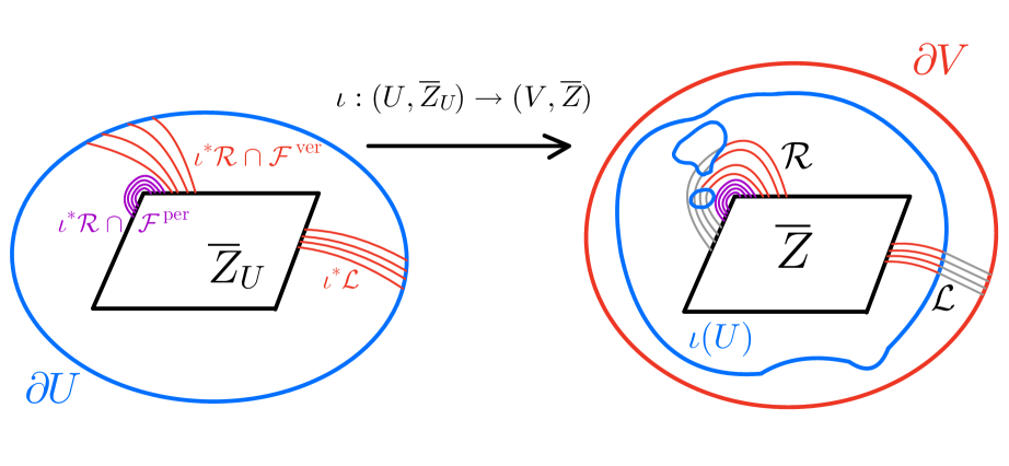
Figure 1. An example of an immersion $\displaystyle\iota$, see also §3.4. A vertical lamination $\displaystyle{\mathcal{L}}$ always lifts to a vertical lamination $\displaystyle\iota^{*}{\mathcal{L}}$. The lift of a peripheral lamination $\displaystyle\mathcal{R}$ can have vertical and peripheral components (§ 3.2).

The width of $\displaystyle F$ is

$${\mathcal{W}}^{\bullet}(F)\coloneqq{\mathcal{W}}(V\setminus\overline{Z}),$$

where $\displaystyle{\mathcal{W}}(V\setminus\overline{Z})=\frac{1}{\operatorname{mod}(V\setminus\overline{Z})}.$ If $\displaystyle{\mathcal{W}}^{\bullet}(F)\leq K$, then $\displaystyle X_{U},~X$ in Item (V) can be selected so that

(2.5) $$\operatorname{mod}(X\setminus\overline{Z})\geq\varepsilon(K).$$

2.2. Iteration $\displaystyle{F^{k}\colon U^{k}\rightrightarrows V}$

We recall from [K, §2.2.2], [DL2, §3.4.6] that $\displaystyle F\colon U\rightrightarrows V$ has the natural fiber product (also known as the $\displaystyle\psi$-restriction, or pullback, or the graph) denoted by

$$F=(f,\iota)\colon U^{2}\rightrightarrows U^{1}=U,{\ \ }{\ \ }\text{ where }{\ \ }U^{2}=\{(x,y)\in U\times U\mid{\ \ }f(y)=\iota(x)\},$$

where $\displaystyle f,\iota\colon U^{2}\rightrightarrows U$ are component-wise projections:

Repeating the construction, we obtain the sequence

$$F\colon U^{k}\rightrightarrows U^{k-1},\hskip 28.45274ptn\geq 1,{\ \ }U^{0}=V,{\ \ }U^{1}=U,$$

together with induced iterations denoted by

(2.6) $$F^{k}=\big(f^{k},\iota^{k}\big)\colon U^{k}\to V.$$

Note that by construction, each $\displaystyle U^{k}$ is conformally a disk, and $\displaystyle f:U^{k}\longrightarrow U^{k-1}$ is a degree $\displaystyle 2$ branched covering.

Note that $\displaystyle\iota\mid U^{k}$ is the lift of $\displaystyle\iota\mid U^{k-1}$ under the covering $\displaystyle f$:

Therefore, Items (IV) and (V) for $\displaystyle\iota\mid U$ from §2.1 imply the following properties for $\displaystyle\iota\mid U^{k}$:

1. for all $\displaystyle n\geq 0$ and all $\displaystyle k>0$, the immersion $\displaystyle\iota\colon U^{k}\to U^{k-1}$ restricts to a homemorphism from $\displaystyle K_{n,U^{k}}\simeq K_{n}$ onto $\displaystyle K_{n,U^{k-1}}\simeq K_{n}$;

1. $\displaystyle\iota\colon U^{k+1}\to U^{k}$ is a covering embedding rel $\displaystyle K_{k+1}$.

Similarly, Item (VI) implies a more general property:

1. for all $\displaystyle n\geq 1$ and $\displaystyle k\geq 0$, the iterats $\displaystyle\iota^{n}\colon U^{n+k}\to U^{k}$ are covering embedding rel $\displaystyle K_{n+k}$.

In other words, $\displaystyle F\colon U^{k}\rightrightarrows U^{k-1}$ is almost a $\displaystyle\psi^{\bullet}$-ql map where Item (V) is replaced by Item (V^k).

Figure 2. Item (IV) in §2.1 prevents overlapping of immersed limbs as illustrated on this figure.

2.3. Inflation of rational maps

In this subsection, we will consider a more general setting of polynomial-like maps (``pl maps'') and demonstrate that $\displaystyle\psi^{\bullet}$-pl Siegel maps naturally emerge by inflation of Siegel prerenormalizations of rational maps; see Proposition 2.3 below. A key assumption about the Siegel prerenormalization (Definition 2.2) is the existence of a partial self-covering restriction (2.8).

In degree $\displaystyle d=2$, Proposition 2.3 constructs a $\displaystyle\psi^{\bullet}$-ql Siegel map satisfying Definition 2.1. We will not provide an axiomatization of $\displaystyle\psi^{\bullet}$-pl Siegel maps in degree $\displaystyle d>2$; Proposition 2.3 should be taken as a guidance, see Remark 2.4.

Assume $\displaystyle g\colon\widehat{\mathbb{C}}\selfmap$ is a rational map with a periodic bounded-type Siegel disk $\displaystyle Z$. By [Zha11], $\displaystyle\overline{Z}$ is a closed qc disk containing at least one critical point on the boundary. Let us fix an iterate

(2.7) $$f\coloneqq g^{p},\hskip 28.45274ptf(\overline{Z})=\overline{Z},$$

preserving the Siegel disk; we do not require $\displaystyle p$ to be the minimal period.

Let us next assume that there is a forward invariant set $\displaystyle{\mathbf{\Upsilon}}=f({\mathbf{\Upsilon}})$ containing the postcritical set of $\displaystyle f$ (which is equal to the postcritical set of $\displaystyle g$) such that $\displaystyle\overline{Z}$ is a connected component of $\displaystyle{\mathbf{\Upsilon}}$. Then

(2.8) $$(f,\ \hookrightarrow)\ \colon\ \widehat{\mathbb{C}}\setminus f^{-1}({\mathbf{\Upsilon}})\ \rightrightarrows\ \widehat{\mathbb{C}}\setminus{\mathbf{\Upsilon}}$$

is a partial self-covering: $\displaystyle f$ represents a covering from a smaller set to a bigger set.

Let $\displaystyle B$ be any open Jordan neighborhood of $\displaystyle\overline{Z}$ such that $\displaystyle{\mathbf{\Upsilon}}\cap B=\overline{Z}$. Let $\displaystyle A$ be a unique component of $\displaystyle f^{-1}(B)$ that contains $\displaystyle\overline{Z}$. If

• $\displaystyle{\mathbf{\Upsilon}}\cap A=\overline{Z},$ and

• $\displaystyle\partial A$ and $\displaystyle\partial B$ are homotopic rel $\displaystyle{\mathbf{\Upsilon}}$,

then we say that $\displaystyle{\mathbf{\Upsilon}}$ is locally saturated at $\displaystyle\overline{Z}$; this notion is independent of the choice of $\displaystyle B$. This implies that $\displaystyle A$ is also a Jordan neighborhood of $\displaystyle\overline{Z}$ and we have a branched covering map

(2.9) $$f=g^{p}\ \colon A\overset{d:1}{\longrightarrow}B$$

restricting to a covering $\displaystyle f\colon A\setminus K_{1}\to B\setminus\overline{Z}$, where $\displaystyle K_{1}\coloneqq[f\mid A]^{-1}(\overline{Z})$.

Definition 2.2 (Siegel prerenormalization).

Assume a rational map $\displaystyle g\colon\widehat{\mathbb{C}}\selfmap$ is endowed with the following data:

• an iterate (2.7) around a Siegel disk $\displaystyle\overline{Z}$,

• a partial self-covering restriction (2.8) so that $\displaystyle{\mathbf{\Upsilon}}$ is locally saturated at $\displaystyle\overline{Z}$.

Then the map

(2.10) $$f=g^{p}\ \colon A\overset{d:1}{\longrightarrow}B$$

a Siegel prerenormalization of $\displaystyle f$ at $\displaystyle\overline{Z}$.

The inflation of (2.10) by means of (2.8) is the extension of $\displaystyle f\colon A\to B$ along all paths in $\displaystyle\widehat{\mathbb{C}}\setminus{\mathbf{\Upsilon}}$; see §2.3.1 for details. We have:

Proposition 2.3 (Inflation of (2.10), see Figure 3).

Consider a rational map $\displaystyle g\colon\widehat{\mathbb{C}}\selfmap$ with a Siegel prerenormalization as in Definition 2.2. Then the inflation of (2.10) by means of (2.8) is a correspondence

(2.11) $$F=(f,\iota)\colon U\rightrightarrows V$$

where

1. $\displaystyle f\colon U\overset{d:1}{\longrightarrow}V$ is a proper branched covering extending $\displaystyle f\colon A\overset{d:1}{\longrightarrow}B$; and

2. $\displaystyle\iota\colon U\longrightarrow V$ is a covering embedding rel $\displaystyle K_{1}$ extending $\displaystyle A\cap B\ \overset{\simeq}{\longrightarrow}\ A\cap B$.
   (In particular, $\displaystyle K_{1}$ is $\displaystyle\iota$-proper.)

Moreover, the iterate

$$F^{k}=(f^{k},\iota^{k})\colon U^{n+k}\rightrightarrows U^{n},\hskip 28.45274ptU^{0}=V$$

is the inflation of

$$f^{k}\ \colon A^{n+k}\ \overset{d^{k}:1}{\longrightarrow}\ A^{n},\hskip 28.45274ptA^{0}=B$$

by means of

$$(f^{k},\ \hookrightarrow)\ \colon\ \widehat{\mathbb{C}}\setminus f^{-n-k}({\mathbf{\Upsilon}})\ \rightrightarrows\ \widehat{\mathbb{C}}\setminus f^{-n}({\mathbf{\Upsilon}}).$$

Here $\displaystyle A^{n}$ is the unique component of $\displaystyle f^{-n}(B)$ containing $\displaystyle\overline{Z}$.

If $\displaystyle d=2$, i.e., $\displaystyle K_{1}$ contains a unique simple critical point, then (2.11) is a $\displaystyle\psi^{\bullet}$-ql Siegel map satisfying Definition 2.1.

The proof of Proposition 2.3 is given in §2.3.1.

Remark 2.4 (Variations of Proposition 2.3).

As we have already mentioned, Proposition 2.3 should be viewed as a guidance in degree $\displaystyle d>2$. Let us mention two possible modifications of the setting.

First, the local saturation condition at $\displaystyle\overline{Z}$ can be relaxed into a local saturation condition at $\displaystyle K_{m}$ for some $\displaystyle m\geq 1$ (i.e., $\displaystyle{\mathbf{\Upsilon}}$ may intersect $\displaystyle K_{m}$ but not $\displaystyle K_{m+1}\setminus K_{m}$).

Second, instead of dealing with the first return map, one can develop the concept of ``$\displaystyle\psi^{\bullet}$-correspondences with multiple connected components''

(2.12) $$F=(f,\iota)\colon\ \Big(\bigcup_{i}U_{i}\Big)\ \rightrightarrows\ \Big(\bigcup_{i}V_{i}\Big)\ \hskip 28.45274ptf\colon U_{i}\to V_{f(i)},{\ \ }\iota\colon U_{i}\to V_{i},$$

where the $\displaystyle U_{i}$ are chosen to contain the original critical points of $\displaystyle g$. (The first return map can significantly increase the number of critical points.) Framework (2.12) is convenient for developing the associated renormalization theory.

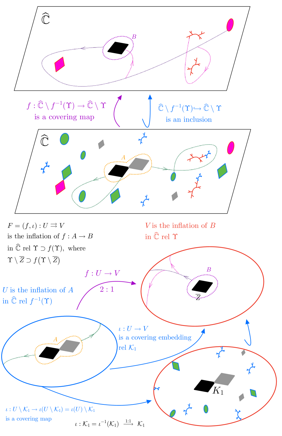
Figure 3. Illustration to Proposition 2.3: the inflation of $\displaystyle f\colon A\to B$ in $\displaystyle\widehat{\mathbb{C}}$ around a Siegel disk $\displaystyle\overline{Z}$ assuming that $\displaystyle{\mathbf{\Upsilon}}$ controls the postcritical set; see §2.3.2 for details regarding the figure.

2.3.1. Inflation: detailed description

Let $\displaystyle V$ be the inflation of $\displaystyle B$ in $\displaystyle\widehat{\mathbb{C}}$ rel $\displaystyle{\mathbf{\Upsilon}}$; the inflation is obtained by extending $\displaystyle B$ along all paths in $\displaystyle\widehat{\mathbb{C}}\setminus{\mathbf{\Upsilon}}$ defined as follows. Let $\displaystyle\mathbb{A}^{0}$ be the universal covering of $\displaystyle\widehat{\mathbb{C}}\setminus{\mathbf{\Upsilon}}$ rel $\displaystyle B^{\prime}\coloneqq B\setminus\partial Z$. This means that $\displaystyle\mathbb{A}^{0}\to\widehat{\mathbb{C}}\setminus{\mathbf{\Upsilon}}$ is a covering that opens up all loops outside of $\displaystyle B^{\prime}$. In particular, $\displaystyle\mathbb{A}^{0}$ is annulus with $\displaystyle\pi_{1}(\mathbb{A}^{0})\simeq\pi_{1}(B^{\prime})$ via $\displaystyle\mathbb{A}^{0}\to\widehat{\mathbb{C}}\setminus{\mathbf{\Upsilon}}$. Note that $\displaystyle\mathbb{A}^{0}$ has a neighborhood boundary component that is conformally identified with $\displaystyle B^{\prime}$. The inflation of $\displaystyle B$ in $\displaystyle\widehat{\mathbb{C}}$ rel $\displaystyle{\mathbf{\Upsilon}}$ is obtained by gluing $\displaystyle\mathbb{A}^{0}$ and $\displaystyle B$ along $\displaystyle B^{\prime}$

$$V=\mathbb{A}^{0}\cup B/\text{\footnotesize$\displaystyle B^{\prime}$}\simeq\mathbb{A}^{0}\sqcup\overline{Z}.$$

Similarly, let $\displaystyle U$ be the inflation of $\displaystyle A$ in $\displaystyle\widehat{\mathbb{C}}$ rel $\displaystyle f^{-1}({\mathbf{\Upsilon}})$:

$$V=\mathbb{A}^{1}\cup A/\text{\footnotesize$\displaystyle A^{\prime}$}\simeq\mathbb{A}^{1}\sqcup K_{1},$$

where $\displaystyle A^{\prime}\coloneqq A\setminus K_{1}$ and $\displaystyle\mathbb{A}^{1}$ is the universal covering of $\displaystyle\widehat{\mathbb{C}}\setminus f^{-1}({\mathbf{\Upsilon}})$ rel $\displaystyle A^{\prime}$. Since $\displaystyle A\setminus K_{1}$ is an annulus, $\displaystyle U\setminus K_{1}$ is an annulus.

The covering map $\displaystyle f\colon A\overset{d:1}{\longrightarrow}B$ lifts to a degree $\displaystyle d$ branched covering map $\displaystyle f:U\longrightarrow V$, and the inclusion map $\displaystyle\iota:\widehat{\mathbb{C}}\setminus f^{-1}({\mathbf{\Upsilon}})\xhookrightarrow{}\widehat{\mathbb{C}}\setminus{\mathbf{\Upsilon}}$ lifts to a covering embedding $\displaystyle\iota:U\longrightarrow V$ rel $\displaystyle K_{1}$.

Since $\displaystyle{\mathbf{\Upsilon}}$ is locally saturated at $\displaystyle\overline{Z}$, the set $\displaystyle K_{1}$ is $\displaystyle\iota$-proper.

Proof of Proposition 2.3.

Item (A) has been justified above.

The local saturation Condition 2.8 implies that, up to homotopy $\displaystyle B$ rel $\displaystyle{\mathbf{\Upsilon}}$, we may assume that $\displaystyle K_{1}\subset A\cap B$. This implies Item (B) by a routine argument.

The claim concerning the iterate is standard; it follows from the naturality of the definition of the inflation.

Assume that $\displaystyle d=2$. Items (I)–(V) of Definition 2.1 are immediate. Item (VI) of Definition 2.1 follows from Item (B) of Proposition 2.3 applied to an iterate of $\displaystyle f$. ∎

2.3.2. Comments to Figure 3

The upper half of the figure illustrates a partial self-covering (2.8). The Siegel disk $\displaystyle\overline{Z}$ from (2.7) is colored in black; its preimage $\displaystyle K_{1}$ under $\displaystyle f\colon A\to B$ is colored in black and gray. Components of $\displaystyle{\mathbf{\Upsilon}}\setminus\overline{Z}$ are colored in red, while components of $\displaystyle f^{-1}({\mathbf{\Upsilon}})\setminus({\mathbf{\Upsilon}}\cup K_{1})$ are colored in green and blue.

The inflation of $\displaystyle f\colon A\to B$ by means of (2.8) is illustrated in the lower half of the figure. The set $\displaystyle V$ is obtained by extending $\displaystyle B$ along all paths in $\displaystyle\widehat{\mathbb{C}}\setminus{\mathbf{\Upsilon}}$; example paths are colored in purple and red. The set $\displaystyle U$ is obtained from by extending $\displaystyle A$ along all paths in $\displaystyle\widehat{\mathbb{C}}\setminus f^{-1}({\mathbf{\Upsilon}})$; example paths are colored in green.

2.4. Examples

Let us discuss how $\displaystyle\psi^{\bullet}$-maps emerge from the rational dynamics. In §2.4.1, we consider the hyperbolic component $\displaystyle\mathcal{H}^{\text{rat}}_{z^{2}}$ of $\displaystyle z\mapsto z^{2}$. The most complicated part of its boundary $\displaystyle\partial H^{\text{rat}}_{z^{2}}$ is where both attracting fixed points become neutral. We give an explicit extraction of $\displaystyle\psi^{\bullet}$-ql maps; the $\displaystyle\iota$-map is, in fact, an inclusion in this case. General hyperbolic components are discussed in §2.4.2 and in §2.4.3.

2.4.1. Matings of neutral quadratic polynomials

Let us illustrate the setting of §2.3 for matings of quadratic polynomials with neutral $\displaystyle\alpha$-fixed points. Such matings arise on the boundary of the hyperbolic component $\displaystyle\mathcal{H}^{\text{rat}}_{z^{2}}$ of $\displaystyle z\mapsto z^{2}$ in the space of quadratic rational maps.

Consider $\displaystyle g\in\partial\mathcal{H}^{\text{rat}}_{z^{2}}$ with two neutral fixed points at $\displaystyle 0$ and $\displaystyle\infty$ that have rotation numbers $\displaystyle\theta_{0},\theta_{\infty}\in\mathbb{R}\setminus\mathbb{Q}$ with $\displaystyle\theta_{0}\not=-\theta_{\infty}$. Assume first that $\displaystyle\theta_{0},\theta_{\infty}\in\Theta_{\mathrm{bnd}}$ are of bounded type. Then $\displaystyle g$ has closed Siegel qc-disks $\displaystyle\overline{Z}_{0},\overline{Z}_{\infty}$ at $\displaystyle 0$ and $\displaystyle\infty$. We set:

• $\displaystyle f_{0}=f_{\infty}\coloneqq g$,

• $\displaystyle{\mathbf{\Upsilon}}_{f_{0}}={\mathbf{\Upsilon}}_{f_{\infty}}={\mathbf{\Upsilon}}\coloneqq\overline{Z}_{0}\cup\overline{Z}_{\infty}$; then the partial self-covering map (2.8) has the form

  (2.13) $$(f_{0}=f_{\infty},=g,\ \ \hookrightarrow)\ \colon\ \widehat{\mathbb{C}}\setminus g^{-1}({\mathbf{\Upsilon}})\ \rightrightarrows\ \widehat{\mathbb{C}}\setminus{\mathbf{\Upsilon}},$$

  where $\displaystyle g^{-1}({\mathbf{\Upsilon}})=g^{-1}(\overline{Z}_{0})\cup g^{-1}(\overline{Z}_{\infty})$ consists of $\displaystyle{\mathbf{\Upsilon}}$ and two prefixed (immediate preimages) Siegel disks;

• $\displaystyle B_{0}$ and $\displaystyle B_{\infty}$ are open Jordan neighborhoods of $\displaystyle\overline{Z}_{0}$ and $\displaystyle\overline{Z}_{\infty}$ such that

  $$B_{0}\cap{\mathbf{\Upsilon}}=\overline{Z}_{0}\hskip 28.45274pt\text{ and }\hskip 28.45274ptB_{\infty}\cap{\mathbf{\Upsilon}}=\overline{Z}_{\infty},$$

• $\displaystyle A_{0}\coloneqq g^{-1}(B_{0})$ and $\displaystyle A_{\infty}\coloneqq g^{-1}(B_{\infty})$ so that

  (2.14) $$f_{0}\equiv g\colon A_{0}\ \overset{2:1}{\longrightarrow}\ B_{0}\hskip 28.45274pt\text{ and }\hskip 28.45274ptf_{\infty}\equiv g\colon A_{\infty}\ \overset{2:1}{\longrightarrow}\ B_{\infty},$$

Then the inflations of maps in (2.14) by means of (2.13) have the following forms:

$$F_{0}=(f_{0}=g,\ \hookrightarrow)\ \colon\ (U_{0},\overline{Z}_{0})\rightrightarrows(V_{0},\overline{Z}_{0}),{\ \ }{\ \ }V_{0}=\widehat{\mathbb{C}}\setminus\overline{Z}_{\infty},\ U_{0}=g^{-1}(V_{0}),$$

$$F_{\infty}=(f_{\infty}=g,\ \hookrightarrow)\ \colon\ (U_{\infty},\overline{Z}_{\infty})\rightrightarrows(V_{\infty},\overline{Z}_{\infty}),{\ \ }{\ \ }V_{\infty}=\widehat{\mathbb{C}}\setminus\overline{Z}_{0},\ U_{\infty}=g^{-1}(V_{\infty})$$

where the immersion $\displaystyle\iota=$``$\displaystyle\hookrightarrow$'' is an embedding. Both $\displaystyle F_{0},F_{\infty}$ are $\displaystyle\psi^{\bullet}$-ql maps.

We have:

(2.15) $${\mathcal{W}}^{\bullet}(F_{0})={\mathcal{W}}^{\bullet}(F_{\infty})={\mathcal{W}}\big(\widehat{\mathbb{C}}\setminus[\overline{Z}_{0}\cup\overline{Z}_{\infty}]\big).$$

By [DLu], $\displaystyle{\mathcal{W}}^{\bullet}(G_{0})$ is bounded in terms of the (combinatorial) distance between $\displaystyle\theta_{0}$ and $\displaystyle-\theta_{\infty}$ and, consequently, such bound for $\displaystyle{\mathcal{W}}^{\bullet}(F_{0})={\mathcal{W}}^{\bullet}(F_{\infty})$ persists for all $\displaystyle\theta_{0},\theta_{\infty}\in\mathbb{R}\setminus\mathbb{Q}$. Consequently, correspondences $\displaystyle F_{0}$ and $\displaystyle F_{\infty}$ can be defined for all such irrational $\displaystyle\theta_{0}\not=-\theta_{\infty}$. For the original $\displaystyle g$, the $\displaystyle 0$ and $\displaystyle\infty$ have disjoint (possibly Cremer) Mother Hedgehogs canonically identified with the Mother Hedgehogs of the associated quadratic polynomials.

2.4.2. Neutral Dynamics at boundaries of hyperbolic components

We expect that the setting of §2.4.1 can be extended, with appropriate refinements and modifications, to all hyperbolic component $\displaystyle\mathcal{H}$ in the space of rational maps with connected Julia sets. Namely, every such $\displaystyle\mathcal{H}$ has a unique postcritically finite (PCF) center $\displaystyle f_{pcf}\in\mathcal{H}$ encoding the combinatorics of $\displaystyle\mathcal{H}$. For $\displaystyle f\in\mathcal{H}$, let us denote by $\displaystyle\mathcal{C}_{f}$ the centers of Fatou components containing either a critical or a postcritical point. If $\displaystyle f=f_{pcf}$, then $\displaystyle\mathcal{C}_{f_{pcf}}$ it is its critical and postcritical set. For $\displaystyle\tau\in\mathcal{C}_{f}$, let $\displaystyle F_{\tau}$ be the Fatou component centered at $\displaystyle\tau$. We naturally have maps

(2.16) $$\big[f_{pcf}\colon F_{\tau}\ \overset{d_{\tau}:1}{\longrightarrow}\ F_{f(\tau)}\big]\ \ \overset{\text{RM}}{\simeq}\ \ \big[z\mapsto z^{d_{\tau}}\ \colon\ \mathbb{D}\overset{d_{\tau}:1}{\longrightarrow}\ \mathbb{D}\big],$$

where $\displaystyle f(\tau)=f_{pcf}(\tau)$ is the image of $\displaystyle\tau$, the identification ``$\displaystyle\ \overset{\text{RM}}{\simeq}\$'' represents a marked Riemann map between $\displaystyle(F_{\tau},\tau)$ and the unit disk $\displaystyle(\mathbb{D},0)$, and the ``$\displaystyle z\mapsto z^{d_{\tau}}$'' represents the Blaschke class of $\displaystyle f_{pcf}\mid F_{\tau}$.

After introducing a finite set of markings for $\displaystyle\mathcal{H}$ to resolve its orbifold points, the set $\displaystyle\mathcal{C}_{f}$ moves holomorphically with $\displaystyle f\in\mathcal{H}$; i.e., $\displaystyle\mathcal{C}_{f}$ is canonically identified between maps in $\displaystyle\mathcal{H}$. Equation (2.16) then takes form

(2.17) $$\big[f\colon F_{\tau,f}\ \overset{d_{\tau}:1}{\longrightarrow}\ F_{f(\tau),f}\big]\ \ \overset{\text{RM}}{\simeq}\ \ \big[B_{\tau,f}\ \colon\ \mathbb{D}\overset{d_{\tau}:1}{\longrightarrow}\ \mathbb{D}\big],$$

where $\displaystyle B_{\tau,f}$ is the Blaschke class of $\displaystyle f$ at $\displaystyle\tau$. The class $\displaystyle B_{\tau,f}$ is trivial if $\displaystyle d_{\tau}=1$. The set of all Blaschke classes $\displaystyle(B_{\tau,f})$ provide a natural parametrization of $\displaystyle\mathcal{H}$. At the boundary $\displaystyle\partial\mathcal{H}$, some of the points in $\displaystyle\mathcal{C}_{f}$ may become neutral.

Conjecture 2.5 (Mother Hedgehog is well defined).

If a periodic $\displaystyle\tau\in\mathcal{C}_{f}$ becomes neutral non-parabolic in the dynamical plane of $\displaystyle f\in\partial\mathcal{H}$, then there is a well-defined periodic Mother Hedgehog $\displaystyle H_{\tau,f}$ centered at $\displaystyle\tau\equiv\tau(f)$. The periodic cycle of $\displaystyle H_{\tau,f}$ contains at least one critical point of $\displaystyle f$. Sector Renormalization provides an $\displaystyle f$-equivariant qc identification of $\displaystyle H_{f}$ with a Mother Hedgehog of some polynomial.

We believe that the theory of $\displaystyle\psi^{\bullet}$-ql maps can be developed to handle Conjecture 2.5.

2.4.3. Disjoint type hyperbolic components

If $\displaystyle\mathcal{H}$ is a hyperbolic component of disjoint type, i.e., any map $\displaystyle f\in\mathcal{H}$ has exactly $\displaystyle 2d-2$ attracting cycles, then the multipliers of non-repelling cycles uniquely parametrize $\displaystyle\mathcal{H}$:

$$\mathcal{H}\ \simeq\ \mathbb{D}^{2d-2};$$

in particular, Blaschke classes in (2.17) are uniquely determined by the multipliers.

Let $\displaystyle g\in\partial\mathcal{H}$ be a rational map with non-repelling periodic cycles $\displaystyle\mathcal{C}_{j}$, $\displaystyle j=1,...,2d-2$ so that the multiplier $\displaystyle\rho_{j}$ is either $\displaystyle|\rho_{j}|<1$ or $\displaystyle\rho_{j}=e^{2\pi i\theta_{j}}$ with $\displaystyle\theta_{j}\in\mathbb{R}/\mathbb{Q}$ of bounded type. Let $\displaystyle\Upsilon$ be the closure of the union of periodic Siegel disks and valuable parts of the periodic attracting components. (Roughly, the latter are bounded by equipotentials though the critical value.) Let $\displaystyle\overline{Z}\subset{\mathbf{\Upsilon}}$ be a Siegel disk with minimal period $\displaystyle p$. Then Proposition 2.3 constructs a $\displaystyle\psi^{\bullet}$-ql Siegel map $\displaystyle F=(f,\iota)\colon U\rightrightarrows V$ by inflation $\displaystyle f=g^{p}$ restricted to a neighborhood of $\displaystyle\overline{Z}$ rel $\displaystyle{\mathbf{\Upsilon}}$ (c.f. [DLu, §3]).

3. Degenerations of $\displaystyle\psi^{\bullet}$-ql maps

Recall that a $\displaystyle\psi^{\bullet}$ Siegel map $\displaystyle F=(f,\iota)\colon U\rightrightarrows V$ consists of a branched covering $\displaystyle f$ and a covering embedding $\displaystyle\iota\colon U\to V$ rel $\displaystyle K_{1}$. In §3.1, we deduce from Item (V) of Definition 2.1 that $\displaystyle\iota$ is, in fact, an embedding on the coastal zone of $\displaystyle K_{1}$ – an open disk bounded by the hyperbolic geodesic. Similarly, using Item (VI^k), an iterate $\displaystyle\iota^{m}\colon U^{m}\to V$ is an embedding in the coastal zone of $\displaystyle K_{m}$.

In §3.2, we introduce full families $\displaystyle{\mathcal{F}}$, outer families $\displaystyle{\mathcal{F}}^{+}$, and various subtypes of the latter, see (3.2). These families play a central role in our analysis of the degeneration of Siegel disks; see  §3.2.2 and §3.2.5 for a brief overview.

We then define the pull-back and push-forward operations on families of arcs and study their properties in § 3.3 and § 3.4, respectively. Note that in $\displaystyle F=f\circ\iota^{-1}$, the $\displaystyle\iota$ is more delicate. In particular, the pushforward $\displaystyle F_{*}=f_{*}\circ\iota^{*}$ is well-defined because $\displaystyle f$ is a branched covering; see Figure 5. On the other hand, within coastal zones, the pullback $\displaystyle F^{*}=\iota_{*}\circ f^{*}$ is essentially just $\displaystyle f^{*}$, which works similarly as for quadratic polynomials.

Finally, we introduce and discuss some modifications required of pseudo-Siegel disks for $\displaystyle\psi^{\bullet}$ maps in §3.5, §3.6, and §3.7.

3.1. Coastal zones

Let $\displaystyle s\geq k$. Consider $\displaystyle K_{s,U^{k}}\subseteq U^{k}$. We define

$$\mathcal{D}^{k}_{s}=\iota^{-k}(V\setminus K_{s,V})\subseteq U^{k}\setminus K_{s,U^{k}}\subseteq U^{k}\setminus K_{k,U^{k}}$$

Since $\displaystyle\iota:U^{k}\setminus K_{k,U^{k}}\longrightarrow\iota\big(U^{k}\setminus K_{k,U^{k}}\big)$ is a covering map by Item (V^k) in § 2.2, and $\displaystyle\iota^{-1}(\iota(\mathcal{D}^{k}_{s}))=\mathcal{D}^{k}_{s}$ we conclude that

$$\iota:\mathcal{D}^{k}_{s}\longrightarrow\iota(\mathcal{D}^{k}_{s})\subseteq\mathcal{D}^{k-1}_{s}$$

is a covering map. We note that $\displaystyle\mathcal{D}^{0}_{s}=V\setminus K_{s,V}$. By Item (VI) in Definition 2.1, we have

(3.1) $$\mathcal{D}^{k}_{k}=U^{k}\setminus K_{k,U^{k}}.$$

Let $\displaystyle\gamma^{k}_{s}$ be the hyperbolic closed geodesic of $\displaystyle\mathcal{D}^{k}_{s}$ representing the simple closed curve around boundary of $\displaystyle K_{s,U^{k}}$. We call the disk in $\displaystyle{\mathcal{C}}^{k}_{s}\subseteq U^{k}$ bounded by $\displaystyle\gamma^{k}_{s}$ the coastal zone. We remark that $\displaystyle{\mathcal{C}}^{0}_{k}\subset{\mathcal{C}}^{0}_{m}$ if $\displaystyle k\leq m$.

Lemma 3.1 ($\displaystyle\iota\colon{\mathcal{C}}^{k}_{s}\hookrightarrow{\mathcal{C}}^{k-1}_{s}$).

For $\displaystyle s\geq k$, the restriction $\displaystyle\iota:{\mathcal{C}}^{k}_{s}\longrightarrow{\mathcal{C}}^{k-1}_{s}$ is injective. Consequently, $\displaystyle\iota^{k}\colon{\mathcal{C}}^{k}_{s}\hookrightarrow{\mathcal{C}}^{0}_{s}\subset V$ is injective.

Proof.

Let $\displaystyle\widetilde{\gamma}^{k-1}_{s}$ be the hyperbolic closed geodesic in $\displaystyle\iota(\mathcal{D}^{k}_{s})$ representing the curve surrounding $\displaystyle K_{k,U^{k-1}}=\iota(K_{k})\subseteq U^{k-1}$. Let $\displaystyle\widetilde{\mathcal{C}}^{k-1}_{s}$ be the disk bounded by $\displaystyle\widetilde{\gamma}^{k-1}_{s}$.

Since $\displaystyle\iota:\mathcal{D}^{k}_{s}\longrightarrow\iota(\mathcal{D}^{k}_{s})=\iota(U^{k})\setminus K_{s,U^{k}}$ is a covering map, $\displaystyle\iota:\gamma^{k}_{s}\longrightarrow\widetilde{\gamma}^{k-1}_{s}$ is a homeomorphism, and $\displaystyle\iota:{\mathcal{C}}^{k}_{s}\longrightarrow\widetilde{\mathcal{C}}^{k-1}_{s}$ is an conformal isomorphism.

Since $\displaystyle\iota(\mathcal{D}^{k}_{s})=\subseteq\mathcal{D}^{k-1}_{s}$, and $\displaystyle\widetilde{\mathcal{C}}^{k-1}_{s}\cap\iota(\mathcal{D}^{k}_{s})=\widetilde{\mathcal{C}}^{k-1}_{s}\cap\mathcal{D}^{k-1}_{s}$, we conclude that $\displaystyle\widetilde{\mathcal{C}}^{k-1}_{s}\subseteq{\mathcal{C}}^{k-1}_{s}$. Therefore, $\displaystyle\iota:{\mathcal{C}}^{k}_{s}\longrightarrow{\mathcal{C}}^{k-1}_{s}$ is injective. ∎

3.2. Families of curves

Recall that degeneration of Riemann surfaces is encoded and analyzed by the extremal width of various families. Following [DL3], we denote by $\displaystyle{\mathcal{F}}$ and $\displaystyle{\mathcal{F}}^{+}$ the full (i.e., in $\displaystyle V$) and outer (i.e., in $\displaystyle V\setminus\overline{Z}$ or in $\displaystyle V\setminus\widehat{Z}^{m}$) families of curves emerging from certain intervals, see §3.2.1 for details. See §3.2.2 and §3.2.5 for a short discussion on how these families are used.

Unlike the case of quadratic polynomials, the outer family $\displaystyle{\mathcal{F}}^{+}$ is further decomposed into the vertical $\displaystyle{\mathcal{F}}^{+,{\operatorname{ver}}}$ and peripheral $\displaystyle{\mathcal{F}}^{+,{\operatorname{per}}}$ parts, see §3.2.3. Finally, in §3.2.4, we decompose the peripheral part $\displaystyle{\mathcal{F}}^{+,{\operatorname{per}}}$ rel $\displaystyle{\mathcal{K}}_{m}$ into the external and diving components. The last decomposition is similar to [DL3, § 2.3.2] with the understanding that curves in $\displaystyle{\mathcal{F}}^{+,{\operatorname{per}}}$ that lift to vertical under $\displaystyle\iota^{\mathfrak{q}_{m+1}}$ are in $\displaystyle{\mathcal{F}}^{+,{\operatorname{per}}}_{{\operatorname{div}},m}$.

All together, we have

(3.2) $$\qquad\qquad{\mathcal{F}}^{+}={\mathcal{F}}^{+,{\operatorname{ver}}}+{\mathcal{F}}^{+,{\operatorname{per}}}-O(1)\\ ={\mathcal{F}}^{+,{\operatorname{ver}}}+{\mathcal{F}}^{+,{\operatorname{per}}}_{{\operatorname{ext}},m}+{\mathcal{F}}^{+,{\operatorname{per}}}_{{\operatorname{div}},m}-O(1).\qquad$$

Decomposition (3.2) is only relevant for parabolic fjords; see §3.2.5.

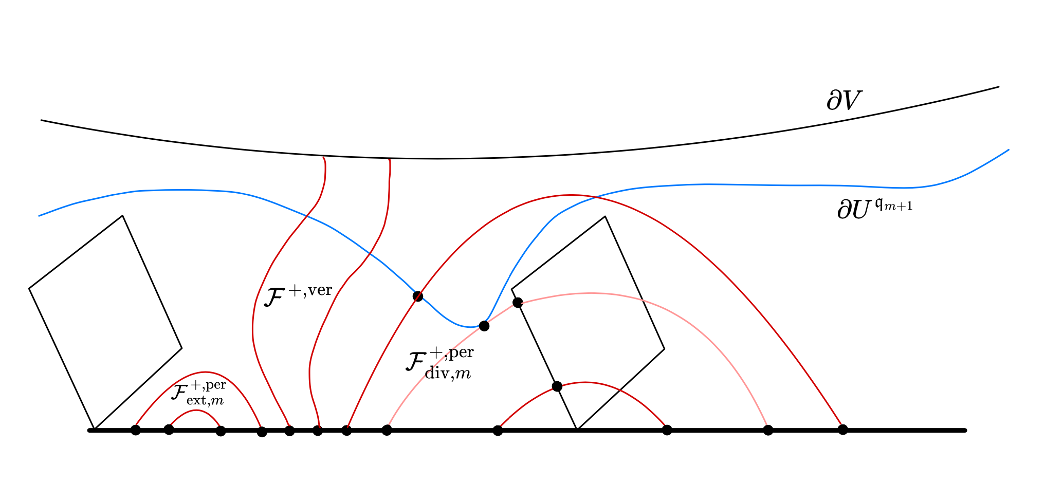
Figure 4. An illustration of the vertical and peripheral families of curves. The peripheral families are further decompose into external and diving components. The diving family may intersect either $\displaystyle\partial U^{\mathfrak{q}_{m+1}}$ or $\displaystyle\mathcal{K}_{m}$.

3.2.1. Full and outer families

Following the notations in [DL3, § 2.3], we consider the following families. Let $\displaystyle I$ be an interval in $\displaystyle\partial Z$. Let $\displaystyle\lambda>1$, and $\displaystyle\lambda I$ be the enlargement of $\displaystyle I$ by attaching two intervals of length $\displaystyle\lambda|I|$ on either side of $\displaystyle I$. We write

$${\mathcal{F}}^{+}_{\lambda}(I)={\mathcal{F}}^{+}_{\lambda,Z}(I):=\{\gamma\subset V\setminus\overline{Z}:\gamma\text{ connects $\displaystyle I$ and $\displaystyle\partial V\cup(\partial Z\setminus\lambda I)$}\}.$$

Similarly, we write

$${\mathcal{F}}_{\lambda}(I)={\mathcal{F}}_{\lambda,Z}(I):=\{\gamma\subset V\setminus(I\cup(\partial Z\setminus\lambda I)):\gamma\text{ connects $\displaystyle I$ and $\displaystyle\partial V\cup(\partial Z\setminus\lambda I)$}\}.$$

Their widths are denoted by $\displaystyle{\mathcal{W}}^{+}_{\lambda}(I)$ and $\displaystyle{\mathcal{W}}_{\lambda}(I)$ respectively.

Let $\displaystyle I$ be an interval in $\displaystyle\partial Z$ and $\displaystyle J$ be an interval in $\displaystyle\partial Z\cup\partial V$. We also write

$${\mathcal{F}}^{+}(I,J):=\{\gamma\subset V\setminus\overline{Z}:\gamma\text{ connects $\displaystyle I$ and $\displaystyle J$}\},$$

and its width by $\displaystyle{\mathcal{W}}^{+}(I,J)$.

3.2.2. Appearance of full families $\displaystyle{\mathcal{F}}$

The full families $\displaystyle{\mathcal{F}}$ are the main objects in the proof of Amplification Theorem 5.1. There, a wide outer family $\displaystyle{\mathcal{F}}^{+}$ is spread around in Lemma 5.2 (an application of the Covering Lemma); the result is a set of wide full families based on the intervals $\displaystyle I^{m}_{s}$; see Items 1 and 2 of Lemma 5.2. In Snake Lair Lemma 5.3, this set of wide families is traded back into an outer wide family with amplification.

It is important that the argument of Theorem 5.1 is applied to pseudo-Siegel disks $\displaystyle{\widehat{Z}}^{m}$ as the boundaries of non-regularized Siegel disks $\displaystyle\overline{Z}$ can have uncontrollable oscillations (Cremer phenomenon in the limit). In general, $\displaystyle{\widehat{Z}}^{m}$ are not $\displaystyle\iota$-proper under $\displaystyle\iota^{k}\colon U^{k}\to V$; this subtlety is resolved in Lemma 3.5 (see also discussion before the lemma).

3.2.3. Vertical and peripheral families

Let $\displaystyle\gamma$ be an proper arc $\displaystyle V-\overline{Z}$. We say it is vertical if $\displaystyle\gamma$ connects a point in $\displaystyle\partial Z$ and a point in $\displaystyle\partial V$. It is peripheral if $\displaystyle\gamma$ connects two points in $\displaystyle\partial Z$.

The family $\displaystyle{\mathcal{F}}^{+}_{\lambda}(I)$ is naturally decomposed into vertical and peripheral subfamilies, and we denote them by

$$\displaystyle{\mathcal{F}}^{+,{\operatorname{ver}}}(I)={\mathcal{F}}^{+,{\operatorname{ver}}}_{Z}(I) \displaystyle:=\{\gamma\in{\mathcal{F}}^{+}_{\lambda}(I):\gamma\text{ connects $\displaystyle I$ and $\displaystyle\partial V$}\},\text{ and }$$

$$\displaystyle{\mathcal{F}}^{+,{\operatorname{per}}}_{\lambda}(I)={\mathcal{F}}^{+,{\operatorname{per}}}_{\lambda,Z}(I) \displaystyle:=\{\gamma\in{\mathcal{F}}^{+}_{\lambda}(I):\gamma\text{ connects $\displaystyle I$ and $\displaystyle\partial Z\setminus\lambda I$}\}.$$

Their extremal widths are denoted by

$${\mathcal{W}}^{+,{\operatorname{ver}}}(I)\text{ and }{\mathcal{W}}^{+,{\operatorname{per}}}_{\lambda}(I^{m})\text{ respectively}.$$

Note that we have

$${\mathcal{F}}^{+,{\operatorname{ver}}}(I)={\mathcal{F}}^{+}(I,\partial V)\text{ and }{\mathcal{F}}^{+,{\operatorname{per}}}_{\lambda}(I)={\mathcal{F}}^{+}(I,\partial Z\setminus\lambda I).$$

The subfamilies $\displaystyle{\mathcal{F}}^{{\operatorname{ver}}}(I),{\mathcal{F}}^{{\operatorname{per}}}_{\lambda}(I)$ of $\displaystyle{\mathcal{F}}_{\lambda}(I)$ and their widths $\displaystyle{\mathcal{W}}^{{\operatorname{ver}}}(I),{\mathcal{W}}^{{\operatorname{per}}}_{\lambda}(I)$ are defined similarly.

3.2.4. External and Diving families

Let $\displaystyle I\subset\partial Z$ and $\displaystyle J\subset\partial V\cup\partial Z$ be two intervals. Fix a level $\displaystyle m$, the family $\displaystyle{\mathcal{F}}^{+}(I,J)$ can be naturally decomposed into two subfamilies:

• the external family relative to level $\displaystyle m$, denoted by $\displaystyle{\mathcal{F}}^{+}_{{\operatorname{ext}},m}(I,J)$: the set of arcs in $\displaystyle{\mathcal{F}}^{+}(I,J)$ that can be lifted under $\displaystyle\iota^{\mathfrak{q}_{m+1}}$ to arcs in $\displaystyle U^{\mathfrak{q}_{m+1}}\setminus{\mathcal{K}}_{m}$ still connecting $\displaystyle I$ and $\displaystyle J$ (see § 3.3);

• the diving family $\displaystyle{\mathcal{F}}^{+}_{{\operatorname{div}},m}(I,J)={\mathcal{F}}^{+}(I,J)\setminus{\mathcal{F}}^{+}_{{\operatorname{ext}},m}(I,J)$ otherwise.

Their widths are denoted by $\displaystyle{\mathcal{W}}^{+}_{{\operatorname{ext}},m}(I,J),{\mathcal{W}}^{+}_{{\operatorname{div}},m}$ respectively. We first remark that

$${\mathcal{W}}^{+}(I,J)={\mathcal{W}}^{+}_{{\operatorname{ext}},m}(I,J)+{\mathcal{W}}^{+}_{{\operatorname{div}},m}(I,J)+O(1).$$

We also use the notation $\displaystyle{\mathcal{F}}^{+,{\operatorname{per}}}_{\lambda,{\operatorname{ext}},m}(I),{\mathcal{F}}^{+,{\operatorname{per}}}_{\lambda,{\operatorname{div}},m}(I)$ for $\displaystyle{\mathcal{F}}^{+}_{{\operatorname{ext}},m}(I,J),{\mathcal{F}}^{+}_{{\operatorname{div}},m}(I,J)$ where $\displaystyle J=\partial Z\setminus\lambda I$.

Note that we have

(3.3) $${\mathcal{W}}^{+}_{\lambda}(I)={\mathcal{W}}^{+,{\operatorname{per}}}_{\lambda,{\operatorname{ext}},m}(I)+{\mathcal{W}}^{+,{\operatorname{per}}}_{\lambda,{\operatorname{div}},m}(I)+{\mathcal{W}}^{+,{\operatorname{ver}}}(I)+O(1)$$

3.2.5. Appearance of outer families $\displaystyle{\mathcal{F}}^{+}$

Outer families $\displaystyle{\mathcal{F}}^{+}$ are the main objects in the analysis of geometries in fjords in Section 4 and 6. Roughly, the external component $\displaystyle{\mathcal{F}}^{+,{\operatorname{per}}}_{{\operatorname{ext}},m}$ is handled by Theorem 4.4 (Log-Rule) while the diving component $\displaystyle{\mathcal{F}}^{+,{\operatorname{per}}}_{{\operatorname{div}},m}$ is handled by Calibration Lemma 6.1. A ``global external input'' is required to genuinely handle the vertical component $\displaystyle{\mathcal{F}}^{+,{\operatorname{ver}}}$; see §6.2 for details.

The theory of snakes [DL3, §6] allows us to convert a full into an outer family. Such a convergence should be executed rel $\displaystyle{\widehat{Z}}^{m}$ as the boundaries of non-regularized Siegel disks $\displaystyle\overline{Z}$ can have uncontrollable oscillations (Cremer phenomenon in the limit). It is important that outer families based on grounded intervals can be easily converted between $\displaystyle\overline{Z}$ and $\displaystyle{\widehat{Z}}^{m}$, see §3.5.6.

3.2.6. Family and width in $\displaystyle U^{k}$

Let $\displaystyle k\leq 10\mathfrak{q}_{m+1}$. We denote $\displaystyle Z_{U^{k}}\subset U^{k}$ be the Siegel disk in $\displaystyle U^{k}$, i.e., the subset so that $\displaystyle\iota^{k}\mid Z_{U^{k}}:Z_{U^{k}}\longrightarrow Z$ is a homeomorphism. Let $\displaystyle I\subset Z_{U^{k}}$. The definition of various families of arcs and their width naturally extends in this case. We add $\displaystyle U^{k}$ in the subscript to denote the objects in $\displaystyle U^{k}$.

For example, we use the notation $\displaystyle{\mathcal{F}}^{+}_{\lambda,U^{k}}(I)={\mathcal{F}}^{+}_{\lambda,Z_{U^{k}},U^{k}}(I)$ to denote the family of arcs $\displaystyle\gamma\subset U^{k}\setminus Z_{U^{k}}$ connecting $\displaystyle I$ and $\displaystyle\partial U^{k}\cup(\partial Z_{U^{k}}\setminus\lambda I)$.

3.2.7. External family in $\displaystyle V$ vs $\displaystyle U^{\mathfrak{q}_{m+1}}$

By definition, $\displaystyle\iota^{\mathfrak{q}_{m+1}}$ lifts univalently the family $\displaystyle{\mathcal{F}}^{+}_{{\operatorname{ext}},m}(I,J)$ into $\displaystyle{\mathcal{F}}^{+}_{U^{\mathfrak{q}_{m+1}}\setminus{\mathcal{K}}_{m}}(I,J)$ – the family of curves in $\displaystyle U^{\mathfrak{q}_{m+1}}\setminus{\mathcal{K}}_{m}$ connecting $\displaystyle I$ and $\displaystyle J$.

Since any limb of $\displaystyle{\mathcal{K}}_{m}\setminus\overline{Z}$ contains a fundamental interval of the abelian covering

$$f^{\mathfrak{q}_{m+1}}\colon U^{\mathfrak{q}_{m+1}}\setminus{\mathcal{K}}_{m}\to V\setminus\overline{Z},$$

wide families can not ``bypass'' any limb. Therefore, the following families in $\displaystyle U^{\mathfrak{q}_{m+1}}\setminus{\mathcal{K}}_{m}$ have width $\displaystyle O(1)$:

• connecting two different interval $\displaystyle T_{1},T_{2}\in{\mathfrak{D}}_{m}$;

• any winding family from $\displaystyle T\in{\mathfrak{D}}_{m}$ to itself.

Therefore, the relevant case is when $\displaystyle I,J\subseteq T=[v,w]\in{\mathfrak{D}}_{m}$. By replacing the family by vertical foliations of geodesic rectangles $\displaystyle\mathcal{R}_{m}(I,J)\subset U^{\mathfrak{q}_{m+1}}\setminus{\mathcal{K}}_{m}$ connecting $\displaystyle I,J$, we have:

$${\mathcal{F}}^{+}_{U^{\mathfrak{q}_{m+1}}\setminus{\mathcal{K}}_{m}}(I,J)-O(1)\subseteq{\mathcal{C}}^{\mathfrak{q}_{m+1}}_{\mathfrak{q}_{m+1}},$$

where $\displaystyle{\mathcal{C}}^{\mathfrak{q}_{m+1}}_{\mathfrak{q}_{m+1}}$ is the coastal zone (see § 3.3). By Lemma 3.1, $\displaystyle\iota^{\mathfrak{q}_{m+1}}$ is injective on $\displaystyle{\mathcal{C}}^{\mathfrak{q}_{m+1}}_{\mathfrak{q}_{m+1}}$. Therefore, $\displaystyle\iota^{\mathfrak{q}_{m+1}}$ maps conformally the geodesic rectangle $\displaystyle\mathcal{R}_{m}(I,J)$ to its image, and we have

$${\mathcal{W}}^{+}_{U^{\mathfrak{q}_{m+1}}\setminus{\mathcal{K}}_{m}}(I,J)={\mathcal{W}}^{+}_{{\operatorname{ext}},m}(I,J)+O(1).$$

3.3. Bistable regions $\displaystyle\boldsymbol{\Xi^{k}_{m}\supset\overline{Z}}$

In this subsection, we will employ properties of coastal zones to justify univalent iterates near $\displaystyle\overline{Z}$.

In §3.3.1, we will adapt the discussion of fjords from [DL3, §2.1.7] to the $\displaystyle\psi^{\bullet}$-setting. Lemma 3.2 describes pullbacks within fjords. In 3.3.2, we discuss pullbacks of rectangles under $\displaystyle f^{k}:U^{k}\setminus K_{k,U^{k}}\longrightarrow V\setminus\overline{Z}$ assuming that rectangles are within coastal zones.

In §3.3.3, we define the $\displaystyle k$th stable part of a fjord under pullbacks. In §3.3.4, we define the $\displaystyle k$th bistable part of a fjord as the $\displaystyle k$th pullback of the $\displaystyle 2k$ stable part under the first return map. Bistable regions $\displaystyle\Xi_{m}^{k}\supset\overline{Z}$ are defined in §3.3.5.

3.3.1. Fjord for $\displaystyle\psi^{\bullet}$-maps and pullbacks $\displaystyle F^{*}=\iota_{*}\ \circ f^{*}$

Below, we adopt the discussion of [DL3, §2.1.7]. As in [DL3], we write

$${\mathcal{K}}_{m}\equiv K_{\mathfrak{q}_{m+1}}=f^{-\mathfrak{q}_{m+1}}(\overline{Z}).$$

Consider an interval $\displaystyle T=[v,w]\in{\mathfrak{D}}_{m},{\ \ }m\geq-1$ in the diffeo-tiling [DL3, §2.1.6]. We also consider intervals $\displaystyle[v^{\prime},w^{\prime}]=f^{\mathfrak{q}_{m+1}}(T)$ and $\displaystyle T^{\prime}=[v^{\prime},w]$ as in [DL3, §2.1.7]. We use the same standing assumption that $\displaystyle f^{\mathfrak{q}_{m+1}}|_{T}$ moves points clockwise towards $\displaystyle w$.

For an interval $\displaystyle J\subset T$, the level $\displaystyle m$-fjord $\displaystyle{\mathfrak{F}}_{m}(J)={\mathfrak{F}}_{m,V}(J)\subset V$ on $\displaystyle J$ is the closed disk bounded by $\displaystyle J$ and the by the hyperbolic geodesic $\displaystyle\gamma^{m}_{J}$ of $\displaystyle V\setminus{\mathcal{K}}_{m}$ with end points $\displaystyle\partial J$ such that $\displaystyle\gamma^{m}_{J}$ is homotopic to $\displaystyle J$ in $\displaystyle V\setminus{\mathcal{K}}_{m}$.

Similarly, for an interval $\displaystyle S\subset[v^{\prime},w^{\prime}]$, the fjords $\displaystyle{\mathfrak{F}}(S)={\mathfrak{F}}_{V}(S)\subset V$ are defined as the closed disk bounded by $\displaystyle S$ and the by the hyperbolic geodesic $\displaystyle\gamma_{S}$ of $\displaystyle V\setminus\overline{Z}$ with end points $\displaystyle\partial S$ such that $\displaystyle\gamma_{S}$ is homotopic to $\displaystyle S$ in $\displaystyle V\setminus\overline{Z}$.

We note that $\displaystyle{\mathfrak{F}}_{m}(J)$ are contained in the coastal zone $\displaystyle{\mathcal{C}}^{0}_{m}$. Thus, the following lemma follows immediately from Lemma 3.1.

Lemma 3.2 ([DL3, Lemma 2.4] for $\displaystyle\psi^{\bullet}$-ql maps).

Using the above notations,
$\displaystyle F^{-\mathfrak{q}_{m+1}}_{T}=\iota^{\mathfrak{q}_{m+1}}\circ[f\mid T]^{-\mathfrak{q}_{m+1}}\colon[v^{\prime},w^{\prime}]\to T$ extends to an injective branch

(3.4) $$F^{-\mathfrak{q}_{m+1}}_{T}\colon\ {\mathfrak{F}}([v^{\prime},w^{\prime}])\ \hookrightarrow\ {\mathfrak{F}}_{m}(T).$$

If $\displaystyle J\subset T^{\prime}$ is a subinterval such that

$$F_{T}^{-t\mathfrak{q}_{m+1}}(J)\subset T^{\prime}{\ \ }\text{ for all }\ t\in\{0,1,\dots,s-1\},{\ \ }{\ \ }\text{ then: }$$

(3.5) $$F_{T}^{-s\mathfrak{q}_{m+1}}\big({\mathfrak{F}}(J)\big)\subset{\mathfrak{F}}_{m}(T);$$

i.e., $\displaystyle{\mathfrak{F}}(J)$ can be lifted under $\displaystyle F^{s\mathfrak{q}_{m+1}}$.

3.3.2. Pullbacks of rectangles under $\displaystyle f^{k}:U^{k}\setminus K_{k,U^{k}}\longrightarrow V\setminus\overline{Z}$

Let $\displaystyle T=[v,w]\in{\mathfrak{D}}_{m}$ be an interval in the diffeo-tiling, and $\displaystyle T^{\prime}=f^{\mathfrak{q}_{m+1}}(T)$. Let $\displaystyle I\subseteq T^{\prime}$ and $\displaystyle J\subseteq\partial Z$ be an interval disjoint from $\displaystyle I$. Let $\displaystyle\mathcal{R}\subseteq V\setminus Z$ be a rectangle with horizontal sides $\displaystyle I,J$. Let $\displaystyle\mathcal{R}_{\text{geod}}(I,J)$ be the geodesic rectangle between $\displaystyle I$ and $\displaystyle J$, i.e., whose vertical sides are geodesics in $\displaystyle V\setminus\overline{Z}$ connecting the corresponding endpoints $\displaystyle\partial I,\partial J$. Up to $\displaystyle O(1)$ of width, we may assume that $\displaystyle\mathcal{R}$ is contained in $\displaystyle\mathcal{R}_{\text{geod}}(I,J)$.

Fix an iterate $\displaystyle f^{k}$ with $\displaystyle k\leq\mathfrak{q}_{m+1}$. Let $\displaystyle I_{-k}\subseteq\overline{Z}$ so that $\displaystyle f^{k}(I_{-k})=I$. Since $\displaystyle f^{k}:U^{k}\setminus K_{k,U^{k}}\longrightarrow V\setminus\overline{Z}$ is a covering, let $\displaystyle\mathcal{R}_{-k}$ be the lift of the rectangle $\displaystyle\mathcal{R}$ in $\displaystyle U^{k}\setminus K_{k,U^{k}}$ that emerges from $\displaystyle I_{-k}$. Note $\displaystyle\mathcal{R}_{-k}$ is contained in the geodesic rectangle of $\displaystyle\mathcal{D}^{k}_{k}=U^{k}\setminus K_{k,U^{k}}$ between $\displaystyle\partial^{h,0}\mathcal{R}_{-k},\partial^{h,1}\mathcal{R}_{-k}$. Thus, $\displaystyle\mathcal{R}_{-k}$ is contained in the coastal zone $\displaystyle{\mathcal{C}}^{k}_{k}$. By Lemma 3.1, $\displaystyle\iota^{k}:{\mathcal{C}}^{k}_{k}\longrightarrow{\mathcal{C}}^{0}_{k}$ is conformal. Let $\displaystyle(F^{k})^{*}(\mathcal{R}):=\iota^{k}(\mathcal{R}_{-k})\subset V\setminus K_{k,V}$, and we call $\displaystyle(F^{k})^{*}(\mathcal{R})$ the pullback of $\displaystyle\mathcal{R}$ under $\displaystyle F^{k}$.

3.3.3. Stable parts $\displaystyle\mathfrak{F}^{k}_{\text{stab}}(T)$ of fjords $\displaystyle\mathfrak{F}(T)$

As before, we assume that $\displaystyle f^{\mathfrak{q}_{m+1}}|_{T}$ moves points clockwise towards $\displaystyle w$, where $\displaystyle T=[v,w]\in{\mathfrak{D}}_{m},{\ \ }m\geq-1$.

Assume that $\displaystyle{\mathfrak{l}}_{m}\geq(k+2){\mathfrak{l}}_{m+1}$. Set $\displaystyle v_{k}=v\boxplus k{\mathfrak{l}}_{m+1}=f^{k\mathfrak{q}_{m+1}}(v)$ and observe that $\displaystyle[v_{k},w]\subset T$. We set

$$\mathfrak{F}_{{\text{stab}}}^{k}(T)\coloneqq\mathfrak{F}([v_{k},w])\ \subset\ \mathfrak{F}(T)$$

and call it the $\displaystyle k$-stable part of the fjord $\displaystyle\mathfrak{F}(T)$.

If $\displaystyle{\mathfrak{l}}_{m}<(k+2){\mathfrak{l}}_{m+1}$, then we set $\displaystyle\mathfrak{F}_{{\text{stab}}}^{k}(T)\coloneqq\emptyset$. By construction,

$$\qquad\mathfrak{F}(T)\equiv\mathfrak{F}_{{\text{stab}}}^{0}(T)\supset\mathfrak{F}_{{\text{stab}}}^{1}(T)\supset\mathfrak{F}_{{\text{stab}}}^{2}(T)\supset\dots\supset\mathfrak{F}_{{\text{stab}}}^{t}(T)=\emptyset\\ \text{if }t>\frac{{\mathfrak{l}}_{m}}{{\mathfrak{l}}_{m+1}}-2.\quad$$

Let us recall that for every $\displaystyle i\leq\mathfrak{q}_{m+1}$ there is an interval $\displaystyle T_{-i}\in{\mathfrak{D}}_{m}$ such that $\displaystyle[f\mid\partial Z]^{-i}$ maps $\displaystyle T$ almost into $\displaystyle T_{-i}$. More precisely, write $\displaystyle T_{-i}=[a,b]$, where $\displaystyle a$ is on the left of $\displaystyle b$ so that $\displaystyle f^{\mathfrak{q}_{m+1}}\mid_{T_{-i}}$ moves points clockwise towards $\displaystyle b$. Write also $\displaystyle[\tilde{v},\tilde{w}]=[f\mid\partial Z]^{-i}(T)$. Then

• either $\displaystyle\tilde{v}=a$ or $\displaystyle\tilde{v}=a\boxminus{\mathfrak{l}}_{m+1}$;

• either $\displaystyle\tilde{w}=b$ or $\displaystyle\tilde{w}=b\boxminus{\mathfrak{l}}_{m+1}$.

Similarly, writing $\displaystyle\tilde{v}_{k}=[f\mid\partial Z]^{-i}(v_{k})$, we have

• either $\displaystyle\tilde{v}_{k}=a_{k}$ or $\displaystyle\tilde{v}_{k}=a_{k}\boxminus{\mathfrak{l}}_{m+1}=a_{k-1}$.

Set

$$\widetilde{\mathfrak{F}}^{k}_{\text{stab}}(T)\coloneqq F_{T}^{-i}\Big(\mathfrak{F}^{k}_{\text{stab}}(T)\Big),\qquad\qquad F_{T}^{-i}\equiv\iota^{i}\circ f_{T}^{-i},$$

where the branch of $\displaystyle F_{T}^{-1}$ is taken along $\displaystyle f^{-i}(T)\approx T_{-i}$. It follows that $\displaystyle\widetilde{\mathfrak{F}}^{k}_{\text{stab}}(T)$ is bounded by the hyperbolic geodesic of $\displaystyle\iota^{i}\big(U^{i}\setminus K_{i}\big)$ and $\displaystyle[\tilde{v}_{k},\tilde{w}]$. Since such a hyperbolic geodesic of $\displaystyle\iota^{i}\big(U^{i}\setminus K_{i}\big)$ is below the assoicated hyperbolic geodesic of $\displaystyle V\setminus\overline{Z}$, we obtain that

(3.6) $$\widetilde{\mathfrak{F}}^{k}_{\text{stab}}(T)\subset\mathfrak{F}([\tilde{v}_{k},\tilde{w}_{k}])\subset{\mathfrak{F}}^{k-1}_{\text{stab}}(T_{-i}).$$

Inclusion (3.6) can be generalized as follows. Consider $\displaystyle i$ with

$$(j-1)\mathfrak{q}_{m+1}<i\leq j\mathfrak{q}_{m+1},\qquad\text{ where }\quad 0<j\leq k.$$

Then

(3.7) $$F^{-i}_{T}\Big(\mathfrak{F}^{k}_{\text{stab}}(T)\Big)\ \subset\ \mathfrak{F}^{k-j}_{\text{stab}}(T_{-i}),\qquad T_{-i}\approx(f\mid_{\partial Z})^{-i}(T),$$

where $\displaystyle F^{-i}_{T}$ is a branch extending $\displaystyle T_{-i}\approx(f\mid_{\partial Z})^{-i}(T)$.

3.3.4. Bistable parts $\displaystyle\Xi_{T}^{k}$ of fjords $\displaystyle\mathfrak{F}(T)$

Using (3.7), we define the $\displaystyle k$th bistable part of a fjord $\displaystyle\mathfrak{(}T)$ as

$$\Xi^{k}_{T}\coloneqq F^{-k\mathfrak{q}_{m+1}}_{T}\Big(\mathfrak{F}_{{\text{stab}}}^{2k}(T)\Big).$$

Clearly,

(3.8) $$\Xi^{k}_{T}\subset\mathfrak{F}^{k}_{\text{stab}}(T)\subset\mathfrak{F}(T).$$

Note that $\displaystyle\Xi^{k}_{T}$ is empty if and only if $\displaystyle{\mathfrak{l}}_{m}<(2k+2){\mathfrak{l}}_{m+1}$. It follows from (3.7) that for every $\displaystyle i\in\mathbb{Z}$ with

$$(j-1)\mathfrak{q}_{m+1}<|i|\leq j\mathfrak{q}_{m+1},\qquad\text{ where }\quad 0<j\leq k,$$

we have

(3.9) $$F^{i}_{T}\Big(\Xi^{k}_{T}\Big)\ \subset\ \Xi^{k-j}_{T_{i}},\qquad T_{i}\approx(f\mid_{\partial Z})^{i}(T),$$

where $\displaystyle F^{i}_{T}$ is a branch extending $\displaystyle T_{i}\approx(f\mid_{\partial Z})^{i}(T)$.

The stable part $\displaystyle\Xi_{T}^{k}$ can also be explicitly defined as follows. In addition to $\displaystyle v_{k}$ specified in §3.3.3, set $\displaystyle w_{k}\coloneqq w\boxminus k{\mathfrak{l}}_{m+1}$ so that $\displaystyle f^{\mathfrak{q}_{m+1}k}(w_{k})=w$. Observe that $\displaystyle v<v_{k}<w_{k}<w$. Let $\displaystyle\gamma$ be the hyperbolic geodesic of $\displaystyle\iota^{k\mathfrak{q}_{m+1}}(U^{k\mathfrak{q}_{m+1}}\setminus K_{k\mathfrak{q}_{m+1}})$ connecting $\displaystyle v_{k}$ and $\displaystyle w_{k}$ that is homotopic to $\displaystyle[v_{k},w_{k}]$ in that space. Then $\displaystyle\Xi^{k}_{T}$ is the component bounded by $\displaystyle\gamma\cup[v_{k},w_{k}]$.

3.3.5. Bistable regions $\displaystyle\Xi_{m}^{k}\supset\overline{Z}$

Given $\displaystyle m\geq-1$, we denote the $\displaystyle k$-th bistable region by

$$\Xi^{k}_{m}:=\overline{Z}\cup\bigcup_{n\geq m}\bigcup_{I\in{\mathfrak{D}}_{n}}\Xi^{k}_{I},\qquad\qquad\Xi^{1}_{m}\equiv\Xi_{m}.$$

Equation (3.9) implies the following. For all $\displaystyle i$ with

$$(j-1)\mathfrak{q}_{m+1}<|i|\leq j\mathfrak{q}_{m+1},\qquad\text{ where }\quad 0<j\leq k,$$

we have the following induced map along $\displaystyle F^{i}\colon\overline{Z}\ \overset{1:1}{\longrightarrow}\ \overline{Z}$:

(3.10) $$F^{i}_{\Xi_{m}^{k}}\equiv\big(f\circ\iota^{-1}\big)^{i}\ \colon\Xi^{k}_{m}\ \overset{1:1}{\longrightarrow}\ F^{i}_{\Xi_{m}^{k}}(\Xi_{m}^{k})\ \subset\ \Xi_{m}^{k-j}.$$

3.4. Transformation rules and univalent push-forward

In this subsection, we state several rules for pushing-forward degeneration along

(3.11) $$(F^{k})_{*}=(f^{k})_{*}\circ(\iota^{k})^{*}\ \colon\ (V,\overline{Z})\ \leadsto\ (U^{k},\overline{Z})\ \leadsto\ (V,\overline{Z}).$$

Univalent pushforward §3.4.1 deals with degenerations outside of the Siegel disk; such a pushforward is applied to laminations in (or emerging from) parabolic fjords.

A simple transformation rule §3.4.2 is obtained by selecting a cutting arc $\displaystyle\gamma$ that connects $\displaystyle\partial Z$ and $\displaystyle\partial V$ and pulling back the associated open disk along $\displaystyle f^{k}$ to obtain a finite-degree restriction for (3.11), see Figure 5. This is also a recipe for a near-degenerate transformation rule relying on the Covering Lemma, see §3.4.3. (In the case of quadratic polynomials, $\displaystyle\gamma$ is selected to connect $\displaystyle{\widehat{Z}}^{m}$ and $\displaystyle\infty$, see [DL3, §8.1.2].)

The simple and near-degenerate transformation rules deal with full degenerations and should be applied for $\displaystyle(V,{\widehat{Z}}^{m})$ instead of $\displaystyle(V,\overline{Z})$. An appropriate modification is presented in §3.6.1; see (3.23) and compare it with (3.11)

3.4.1. Univalent push-forward

We now explain the construction of univalent push-forward of a rectangle. We refer the readers to [DL3, §2.3.3] for the quadratic polynomial setting. Let $\displaystyle T=[v,w]\in{\mathfrak{D}}_{m},{\ \ }m\geq-1$ in the diffeo-tiling [DL3, §2.1.6]. Consider a rectangle $\displaystyle\mathcal{R}\subseteq V\setminus Z$ with $\displaystyle\partial^{h,0}\mathcal{R}\subset T$ and $\displaystyle\partial^{h,1}\mathcal{R}\subseteq\partial Z\cup\partial V$. Let us fix an iterate $\displaystyle f^{i}$ with $\displaystyle i\leq\mathfrak{q}_{m+1}$. We will now describe the univalent push-forward under $\displaystyle f^{i}$.

Let $\displaystyle\mathcal{F}(\mathcal{R})$ be the lamination of the vertical arcs in $\displaystyle\mathcal{R}$. Let $\displaystyle\mathcal{F}_{U^{i}}$ be the lift of $\displaystyle\mathcal{F}(\mathcal{R})$ under $\displaystyle\iota^{i}$ that emerges from $\displaystyle\overline{Z}$ Let $\displaystyle\mathcal{F}_{U^{i}}^{\prime}$ be the restriction of $\displaystyle\mathcal{F}_{U^{i}}$ in $\displaystyle U^{i}-K_{i,U^{i}}$: the family $\displaystyle\mathcal{F}_{U^{i}}^{\prime}$ consists of subarcs $\displaystyle\gamma^{\prime}$ of $\displaystyle\gamma\in\mathcal{F}_{U^{i}}$ such that every $\displaystyle\gamma^{\prime}$ is the shortest subarc of $\displaystyle\gamma$ connecting $\displaystyle\partial^{h,0}\mathcal{R}$ to $\displaystyle\partial K_{i,U^{i}}\cup\partial U^{i}$. Note that arcs in $\displaystyle\mathcal{R}_{U^{i}}^{\prime}$ form three different types: left, right or vertical. Thus, we obtain at most three rectangles by considering the region bounded by the leftmost and rightmost curves (see [DL3, A.1.8]). Denote them by $\displaystyle\mathcal{R}_{l,U^{i}},\mathcal{R}_{r,U^{i}},\mathcal{R}_{{\operatorname{ver}},U^{i}}$. Let $\displaystyle\widetilde{\mathcal{R}}_{l,U^{i}},\widetilde{\mathcal{R}}_{r,U^{i}},\widetilde{\mathcal{R}}_{{\operatorname{ver}},U^{i}}$ be the sub-rectangles obtained from $\displaystyle\mathcal{R}_{l,U^{i}},\mathcal{R}_{r,U^{i}},\mathcal{R}_{{\operatorname{ver}},U^{i}}$ by removing the $\displaystyle 1$-buffers on every side. Let $\displaystyle\widetilde{\mathcal{R}}_{U^{i}}=\widetilde{\mathcal{R}}_{l,U^{i}}\cup\widetilde{\mathcal{R}}_{r,U^{i}}\cup\widetilde{\mathcal{R}}_{{\operatorname{ver}},U^{i}}$. Note that $\displaystyle{\mathcal{W}}(\widetilde{\mathcal{R}}_{U^{i}})\geq{\mathcal{W}}(\mathcal{R})-12$. Then by [DL3, Lemma A.8], we have that the map

(3.12) $$f^{i}:\widetilde{\mathcal{R}}_{U^{i}}\longrightarrow f^{i}(\widetilde{\mathcal{R}}_{U^{i}})\subset V\setminus Z$$

is injective.

We refer to (3.12) the univalent push-forward of $\displaystyle\mathcal{R}$. We also denote the image by $\displaystyle F^{i}_{*}(\mathcal{R})=f^{i}_{*}\circ(\iota^{k})^{*}(\mathcal{R})=f^{i}(\widetilde{\mathcal{R}}_{U^{i}})$.

3.4.2. Simple transformation rule of $\displaystyle{\mathcal{W}}({\mathcal{L}})$

We now discuss a different construction suitable for the application of the covering lemma.

Let $\displaystyle I\subset\partial Z$, and $\displaystyle\tau>1$. Let $\displaystyle{\mathcal{L}}$ be a lamination consisting of arcs in $\displaystyle V\setminus(I\cup(\partial Z\setminus\tau I))$ connecting $\displaystyle I$ to $\displaystyle\partial V\cup(\partial Z\setminus\tau I)$. We will now describe the simple transfer of the width family $\displaystyle{\mathcal{L}}$ under $\displaystyle f^{k}$.

Let $\displaystyle I_{k}=(F|_{\partial Z})^{k}(I)$. Let $\displaystyle\gamma_{k}\subseteq V$ be a curve connecting $\displaystyle\partial Z\setminus\tau I_{k}$ to $\displaystyle\partial V$ (see Figure 5). Denote $\displaystyle Y:=V\setminus(\gamma_{k}\cup(\partial Z\setminus\tau I_{k}))$. Note that $\displaystyle Y$ is a disk. Let $\displaystyle X$ be the component of $\displaystyle f^{-k}(Y)\subseteq U^{k}$ that contains $\displaystyle I$, and let $\displaystyle\iota^{k}(X)$. Let $\displaystyle{\mathcal{L}}^{\prime}$ be the restriction in $\displaystyle\iota^{k}(X)$ of the family $\displaystyle{\mathcal{L}}$ emerging from $\displaystyle I$. Then we can lift the lamination $\displaystyle{\mathcal{L}}^{\prime}$ via $\displaystyle\iota^{k}$ and obtain a lamination $\displaystyle\widetilde{{\mathcal{L}}}$ in $\displaystyle X$ connecting $\displaystyle I$ to $\displaystyle\partial X$. Note that $\displaystyle{\mathcal{W}}(\widetilde{{\mathcal{L}}})\geq{\mathcal{W}}({\mathcal{L}})$. Thus, this gives a lower bound for the modulus of the annulus $\displaystyle X\setminus I\subseteq U^{k}$

(3.13) $${\mathcal{W}}(X\setminus I)\geq{\mathcal{W}}({\mathcal{L}}).$$

Now suppose that

1. the width of the family of arcs connecting $\displaystyle I_{k}$ to $\displaystyle\gamma_{k}$ in $\displaystyle V\setminus(I_{k}\cup\gamma_{k}\cup(\partial Z\setminus\tau I_{k}))$ is $\displaystyle O(1)$, which can be achieved by choosing $\displaystyle\gamma_{k}$ carefully under mild modifications, see [DL3, §8.1.5]; in particular, such a $\displaystyle\gamma_{k}$ can be selected if $\displaystyle f(\tau I_{k})$ is disjoint from $\displaystyle\tau I_{k}$;

2. the degree of the branched covering $\displaystyle f^{k}:X\longrightarrow Y$ is $\displaystyle D$, which can be bounded in terms of $\displaystyle\tau$ (see [DL3, §8.1.2])

Remark 3.3.

The disjointness assumption between $\displaystyle f(\tau I_{k})$ and $\displaystyle\tau I_{k}$ in (1) leads to the combinatorial assumption ``$\displaystyle|I|\leq|\theta_{0}|/(2{\boldsymbol{\lambda}}_{\mathbf{t}})$'' in Amplification Theorem 5.1, where $\displaystyle\tau={\boldsymbol{\lambda}}_{k}$ is big.

In the proof of Lemma 6.4, we will apply the simple transformation rule with $\displaystyle\tau=3$ (after projecting the degeneration to $\displaystyle{\widehat{Z}}^{m}$). There, the disjointness assumption can be relaxed into the disjointness between $\displaystyle f^{i}(\tau I_{k})$ and $\displaystyle\tau I_{k}$ for $\displaystyle i\leq 7$. If there are less than $\displaystyle 7$ combinatorial intervals, then the selection of $\displaystyle\gamma_{k}$ is not required.

Let $\displaystyle F_{\tau}(I_{k})$ be the family of arcs in $\displaystyle V\setminus(I_{k}\cup(\partial Z\setminus\tau I_{k}))$ connecting $\displaystyle I_{k}$ to $\displaystyle\partial V\cup(\partial Z\setminus\tau I_{k})$. Then we get

$${\mathcal{W}}_{\tau}(I_{k}):={\mathcal{W}}(F_{\tau}(I_{k}))\geq{\mathcal{W}}(Y\setminus I_{k})-O(1)\geq\frac{{\mathcal{W}}(X\setminus I)}{D}-O(1)\geq\frac{{\mathcal{W}}({\mathcal{L}})}{D}-O(1).$$

In particular, if $\displaystyle{\mathcal{W}}({\mathcal{L}})$ is big, then we also obtain a large lamination $\displaystyle{\mathcal{L}}_{k}$ of $\displaystyle F_{\tau}(I_{k})$ whose width is at least by $\displaystyle\frac{{\mathcal{W}}({\mathcal{L}})}{D}-O(1)$. We call such a construction the simple transformation rule of $\displaystyle{\mathcal{W}}({\mathcal{L}})$.

3.4.3. Near-degenerate transformation rule of $\displaystyle{\mathcal{W}}({\mathcal{L}})$

Let us assume the setup of § 3.4.2. Suppose $\displaystyle\tau\gg 1$, Then the degree $\displaystyle D$ in Condition 2 is also large. In this setting, we use the following modification. We define $\displaystyle B:=V\setminus(\gamma_{k}\cup(\partial Z\setminus 10I_{k}))$, and let $\displaystyle A$ be the component of $\displaystyle f^{-k}(B)$ that contains $\displaystyle I$. Then $\displaystyle f^{k}:(X,A,I)\longrightarrow(Y,B,I_{k})$ is a branched covering between nested Jordan disks. This sets up the application of the covering lemma (see [DL3, §8.1, Lemma 8.5] and [KL1] for more details). We call such a construction that involves the covering lemma the near-degenerate transformation rule of $\displaystyle{\mathcal{W}}({\mathcal{L}})$.

Figure 5. Pushforward of $\displaystyle{\mathcal{F}}_{\tau}(I)$ under the branched covering. Observe that $\displaystyle Y\coloneqq V\setminus\big[\gamma\cup(\tau I_{k})^{c}\big]$ is a disk.

3.5. Pseudo-Siegel disks

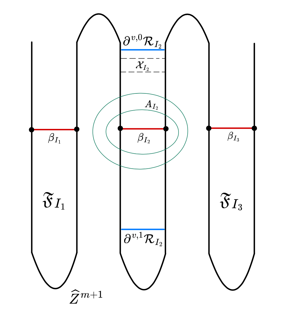
Figure 8. An illustration of the regularization $\displaystyle{\widehat{Z}}^{m+1}\leadsto{\widehat{Z}}^{m}$ in the rectangle $\displaystyle\mathcal{R}$.

The definition of level $\displaystyle m$ pseudo-Sigel disk $\displaystyle{\widehat{Z}}^{m}$ for a $\displaystyle\psi^{\bullet}$-ql Siegel map is the same as for quadratic polynomials (see [DL3, Definition 5.1]) with the understanding that all auxiliary objects at level $\displaystyle m$ (such as channels, dams, collars and protections) defined in [DL3, § 5.1] (see Figure 8, or [DL3, Figure 16]) are contained in the bistable region $\displaystyle\Xi_{m}\equiv\Xi^{1}_{m}$ sepcified in §3.3.5.

Given a peripheral curve $\displaystyle\beta\subset V\setminus Z$ with endpoints in $\displaystyle I$, where $\displaystyle I\in\mathcal{D}_{m}$, set $\displaystyle\widehat{\mathfrak{F}}_{\beta}$ to be the closure of the connected component of $\displaystyle V\setminus(Z\cup\beta)$ enclosed by $\displaystyle\beta\cup I$. If $\displaystyle\widehat{\mathfrak{F}}_{\beta}$ is peripheral rel $\displaystyle\overline{Z}$, then we call $\displaystyle\widehat{\mathfrak{F}}_{\beta}$ the parabolic fjord bounded by $\displaystyle\beta$; see Figure 8. We will refer to $\displaystyle\beta$ as the dam of $\displaystyle\widehat{\mathfrak{F}}_{\beta}$. If $\displaystyle\beta$ is a hyperbolic geodesic of $\displaystyle V\setminus\overline{Z}$, then we say that the fjord $\displaystyle\widehat{\mathfrak{F}}_{\beta}$ is geodesic.

Let us state a definition of pseudo-Siegel disks with slightly simplified notations. In particular, outer protections $\displaystyle\mathcal{X}_{I}$ are considered below rel $\displaystyle\overline{Z}$ instead of $\displaystyle\widehat{Z}^{m+1}$ as it was in [DL3, Assumption 6]. (Protecting rectangle rel $\displaystyle\overline{Z}$ can be easily projected into a protecting rectangle rel $\displaystyle{\widehat{Z}}^{m+1}$ and vise-versa, see [DL3, Lemma 5.9].)

Definition 3.4.

A pseudo-Siegel disk $\displaystyle\widehat{Z}^{m}\subseteq\Xi_{m}\subset V$ of $\displaystyle m\geq-1$ and its territory $\displaystyle{\widehat{Z}}^{m}\subset\mathcal{X}({\widehat{Z}}^{m})\subset\Xi_{m}$ are disks inductively constructed as follows (from bigger $\displaystyle m$ to smaller ones):

1. $\displaystyle\widehat{Z}^{m}=\overline{Z}$ and $\displaystyle\mathcal{X}(\widehat{Z}^{m})=\overline{Z}$ for all sufficiently large $\displaystyle m\gg 0$,

2. either

   $$\widehat{Z}^{m}:=\widehat{Z}^{m+1}\text{ and }\mathcal{X}(\widehat{Z}^{m}):=\mathcal{X}(\widehat{Z}^{m+1}),$$

   or for every interval $\displaystyle I\in\mathfrak{D}_{m}$ there is

   • a parabolic fjord $\displaystyle\widehat{\mathfrak{F}}_{I}\equiv\widehat{\mathfrak{F}}_{\beta_{I}}$ bounded by its dam $\displaystyle\beta_{I}$ with endpoints in $\displaystyle I$; and

   • a rectangle $\displaystyle\mathcal{X}_{I}$ protecting $\displaystyle\widehat{\mathfrak{F}}_{I}$, i.e., $\displaystyle\widehat{\mathfrak{F}}_{I}\subset\overset{\bullet}{\mathcal{X}}{}_{I}$,

   such that

   (3.14) $$\widehat{Z}^{m} =\widehat{Z}^{m+1}\cup\bigcup_{I\in\mathfrak{D}_{m}}\widehat{\mathfrak{F}}_{I}$$

   $$\mathcal{X}\big(\widehat{Z}^{m}\big) =\mathcal{X}({\widehat{Z}}^{m+1})\cup\bigcup_{I\in\mathfrak{D}_{m}}\overset{\bullet}{\mathcal{X}}{}_{I}$$

   and such that $\displaystyle{\widehat{Z}}^{m}$ and $\displaystyle\mathcal{X}\big(\widehat{Z}^{m}\big)$ satisfy $\displaystyle 7$ compatibility condition stated in [DL3, § 5.1].

Here $\displaystyle\overset{\bullet}{\mathcal{X}}{}$ the union of $\displaystyle\mathcal{X}$ and the closure of the connected component of $\displaystyle V\setminus(\mathcal{X}\cup\overline{Z})$ enclosed by $\displaystyle\partial^{v}\mathcal{X}\cup\overset{\circ}{I}$, where $\displaystyle\overset{\circ}{I}$ is $\displaystyle I$ without its endpoints. (Removing the endpoints is relevant if $\displaystyle m=-1$.)

It follows that $\displaystyle\widehat{\mathfrak{F}}_{I}\subset\Xi_{m}$ that $\displaystyle\widehat{\mathfrak{F}}_{I}\subset\Xi_{I}\subset\mathfrak{F}(I)$, see (3.8).

3.5.1. Bistability of $\displaystyle{\widehat{Z}}^{m}$

Given a pseudo-Siegel disk $\displaystyle{\widehat{Z}}^{m}$, its bistability $\displaystyle{\text{bistab}}({\widehat{Z}}^{m})$ is the smallest number $\displaystyle k$ so that $\displaystyle\mathcal{X}({\widehat{Z}}^{m})\subset\Xi_{m}^{k+1}$. It follows that for every $\displaystyle i$ with $\displaystyle|i|\leq\mathfrak{q}_{m+1}k$, the induced image

(3.15) $${\widehat{Z}}^{m}_{*i}\coloneqq F^{i}_{\Xi_{m}^{k}}({\widehat{Z}}^{m}),\qquad\qquad F^{i}_{\Xi_{m}^{k}}\mid_{\Xi_{m}^{k}}\ \ \text{is in ~\eqref{eq:F_biXi}}$$

is also a pseudo-Siegel disk satisfying Definition 3.4 with territory

$$\mathcal{X}({\widehat{Z}}^{m}_{*i})=F^{i}_{\Xi_{m}^{k}}\big(\mathcal{X}({\widehat{Z}}^{m})\big)\subset\Xi_{m}.$$

3.5.2. Geodesic pseudo-Siegel disks

We say that a pseudo-Siegel disk $\displaystyle{\widehat{Z}}^{m}$ is geodesic if

• all the auxiliary objects are hyperbolic geodesics in either $\displaystyle V\setminus\overline{Z}$ or $\displaystyle{\widehat{Z}}^{m}$; we refer the readers to [DL3, § 5.1.9] for more details; in particular, $\displaystyle{\widehat{Z}}^{m}$ is obtained by adding geodesic fjords;

• $\displaystyle{\text{bistab}}({\widehat{Z}}^{m})\geq 10$.

3.5.3. Remarks about stability and bistability

In [DL3, § 5.1.8], the notion of stability $\displaystyle{\text{stab}}({\widehat{Z}}^{m})$ was introduced for pseudo-Siegel disks $\displaystyle{\widehat{Z}}^{m}$ in terms of combinatorial distances between the endpoints of $\displaystyle I$ and $\displaystyle\mathcal{X}_{I}\cap I$. [DL3, Lemma 5.4] implies the stability of $\displaystyle{\widehat{Z}}^{m}$ under pulling-back.

In the current paper, we find it more natural to consider bistability instead of stability. Consequently, the notion of geodesic pseudo-Siegel disks in §3.5.2 is slightly stronger than the associated notion in [DL3, § 5.1.9].

Exponentially big bistability occurs inside a deep part of the parabolic fjords $\displaystyle{\mathfrak{F}}([\tilde{x},\tilde{y}])$, see Lemma 4.6. Consequently, we will show in §7.3.4 that pseudo-Siegel disks $\displaystyle{\widehat{Z}}^{m}$ constructed in Theorem 1.3 have bistability $\displaystyle\geq e^{\sqrt{\mathbf{K}}}$, where $\displaystyle{\mathbf{K}}\gg 1$ is a big constant representing $\displaystyle O(1)$ in Item (A) of Theorem 1.2. In other words, pseudo-Siegel disks naturally come with arbitrary large (by increasing $\displaystyle{\mathbf{K}}$) bistability.

3.5.4. Types of intervals on $\displaystyle\partial{\widehat{Z}}^{m}$

An interval $\displaystyle I^{m}\subseteq\partial{\widehat{Z}}^{m}$ is regular if its endpoints are contained in $\displaystyle\partial{\widehat{Z}}^{m}\cap\partial Z$, and is grounded if it is regular and its endpoints are away from the inner-buffers (see [DL3, § 5.2.3]). Let $\displaystyle I\subset\partial Z$ be an interval. It is regular rel $\displaystyle{\widehat{Z}}^{m}$ if its endpoints are contained in $\displaystyle\partial{\widehat{Z}}^{m}\cap\partial Z$. For a regular interval $\displaystyle I$, its projection $\displaystyle I^{m}\subseteq\partial{\widehat{Z}}^{m}$ is the interval on $\displaystyle\partial{\widehat{Z}}^{m}$ with the same end point and the same orientation as $\displaystyle I$. For a general interval $\displaystyle I\subset\partial Z$, its projection is the projection of the smallest regular interval that contains $\displaystyle I$. An interval $\displaystyle I$ is grounded rel $\displaystyle{\widehat{Z}}^{m}$ if its projection $\displaystyle I^{m}\subseteq\partial{\widehat{Z}}^{m}$ is grounded. The well-grounded intervals can be defined in the exact same way as [DL3, § 5.2.2].

We note that grounded intervals are used in the formalization of the Log-Rules for $\displaystyle\operatorname{int}({\widehat{Z}}^{m})$ [DL3, §5.3, §5.4] and of the snake theory [DL3, §6].

3.5.5. Families of curves for pseudo-Siegel disks

We remark that the definition in § 3.2 naturally extends to the pseudo-Siegel disks, by taking projections. For example, let $\displaystyle I$ be a regular interval in $\displaystyle\partial Z$, with projection $\displaystyle I^{m}\subset{\widehat{Z}}^{m}$. We denote by $\displaystyle{\mathcal{F}}^{+}_{\lambda}(I^{m})={\mathcal{F}}^{+}_{\lambda,{\widehat{Z}}^{m}}(I^{m})$ the family of arcs in $\displaystyle V\setminus{\widehat{Z}}^{m}$ that connects $\displaystyle I^{m}$ and $\displaystyle\partial V\cup(\partial{\widehat{Z}}^{m}\setminus(\lambda I)^{m})$. The vertical, peripheral, external and diving subfamilies are defined accordingly.

3.5.6. Outer geometry of $\displaystyle{\widehat{Z}}$

Under certain minor conditions, outer families rel $\displaystyle\partial Z$ and $\displaystyle\partial{\widehat{Z}}^{m}$ can be easily converted into each other, see (3.16), (3.17), and (3.18) below. The conversion is based on [DL3, §5.2]; here we summarize details. Below, we will compare the geometries of $\displaystyle V\setminus\overline{Z}$ and $\displaystyle V\setminus{\widehat{Z}}^{m}$. A somewhat similar comparison between $\displaystyle U^{k}\setminus{\widehat{Z}}^{m}$ and $\displaystyle\widehat{U}^{k}\setminus{\widehat{Z}}^{m}$ is discussed in Lemma 3.5.

Given an interval $\displaystyle I^{m}\subset\partial{\widehat{Z}}^{m}$, let $\displaystyle I^{m,{\operatorname{grnd}}}\subset I^{m}$ be the biggest grounded subinterval within $\displaystyle I^{m}$. Then $\displaystyle I^{m}\setminus I^{m,{\operatorname{grnd}}}$ has at most two components; each of these components is protected by an annulus with a definite modulus. It easily follows (see [DL3, Lemma 5.18]) that if $\displaystyle\operatorname{dist}(I^{m},J^{m})\geq{\mathfrak{l}}_{m}$, then

$${\mathcal{W}}(I^{m},J^{m})={\mathcal{W}}(I^{m,{\operatorname{grnd}}},J^{m,{\operatorname{grnd}}})+O(1).$$

Given $\displaystyle I\subset\partial Z$, let $\displaystyle I^{\operatorname{grnd}}\subset I$ be the biggest regular subinterval of $\displaystyle I$ such that the projection $\displaystyle I^{m,{\operatorname{grnd}}}$ of $\displaystyle I^{\operatorname{grnd}}$ onto $\displaystyle\partial{\widehat{Z}}^{m}$ is grounded. Using [DL3, Lemma 5.10], we obtain:

(3.16) $$\qquad{\mathcal{W}}^{+}_{Z}(I,J)={\mathcal{W}}^{+}_{Z}(I^{{\operatorname{grnd}}},J^{\operatorname{grnd}})+O(1)=\\ {\mathcal{W}}^{+}_{{\widehat{Z}}^{m}}(I^{m,{\operatorname{grnd}}},J^{m,{\operatorname{grnd}}})+O(1),\qquad$$

and

(3.17) $$\qquad{\mathcal{W}}^{+}_{Z}(I,\partial V)={\mathcal{W}}^{+}_{Z}(I^{{\operatorname{grnd}}},\partial V)+O(1)=\\ {\mathcal{W}}^{+}_{{\widehat{Z}}^{m}}(I^{m,{\operatorname{grnd}}},\partial V)+O(1).\qquad$$

Consequently,

(3.18) $$\qquad{\mathcal{W}}^{+}_{\lambda,Z}(I)={\mathcal{W}}^{+}_{Z}\big(I,(\lambda I)^{c}\big)+{\mathcal{W}}^{+}_{Z}(I,\partial V)-O(1)=\\ {\mathcal{W}}^{+}_{{\widehat{Z}}^{m}}\left(I^{m,{\operatorname{grnd}}},\ \Big(\lambda I)^{c}\Big)^{m,{\operatorname{grnd}}}\right)+{\mathcal{W}}^{+}_{{\widehat{Z}}^{m}}(I^{m,{\operatorname{grnd}}},\partial V)+O(1).\qquad$$

To simplify notations, let us denote the second line in (3.18) as

(3.19) $$\qquad{\mathcal{W}}\big({\operatorname{proj}}^{+,{\operatorname{grnd}}}_{\lambda,V,{\widehat{Z}}^{m}}(I)\big)\equiv{\mathcal{W}}\Big({\operatorname{proj}}^{\operatorname{grnd}}_{V,{\widehat{Z}}^{m}}\big({\mathcal{F}}^{+}_{\lambda,Z}(I)\big)\Big)\coloneqq\\ {\mathcal{W}}^{+}_{{\widehat{Z}}^{m}}\left(I^{m,{\operatorname{grnd}}},\ \Big((\lambda I)^{c}\Big)^{m,{\operatorname{grnd}}}\right)+{\mathcal{W}}^{+}_{{\widehat{Z}}^{m}}(I^{m,{\operatorname{grnd}}},\partial V),\qquad$$

where $\displaystyle{\operatorname{proj}}_{V,{\widehat{Z}}^{m}}\big({\mathcal{F}}^{+}_{\lambda,Z}(I)\big)$ is the projection of the family $\displaystyle{\mathcal{F}}^{+}_{\lambda,Z}(I)$ into $\displaystyle V\setminus\overline{Z}$. Then (3.18) takes form

(3.20) $${\mathcal{W}}^{+}_{\lambda,Z}(I)\ =\ {\mathcal{W}}\big({\operatorname{proj}}^{+,{\operatorname{grnd}}}_{\lambda,V,{\widehat{Z}}^{m}}(I)\big)+O(1)$$

We remark that the class of grounded intervals in (3.16), (3.17), (3.18) is selected for convenience. For instance, instead of $\displaystyle I^{m,{\operatorname{grnd}}}\subset I^{m}$, one can specify a combinatorially smaller (more ``optimal'') subinterval $\displaystyle I^{\prime m}\subset I^{m,{\operatorname{grnd}}}$ by considering the biggest subinterval $\displaystyle I^{\prime m}\subset I^{m}$ whose endpoints are outside of (the boundary of) any fjord $\displaystyle{\mathfrak{F}}^{m}_{I}$ appearing in (3.14).

3.6. Lifting from $\displaystyle(V,\widehat{Z}^{m})$ to $\displaystyle(U^{k},\widehat{Z}^{m}_{U^{k}})$ under $\displaystyle\iota^{k}$

As we have already mentioned, in the near-degenerate regime, $\displaystyle\psi^{\bullet}$-ql maps are quite similar to ql maps. Figure 1 illustrates an immersion $\displaystyle\iota\colon U\to V$ defined around a $\displaystyle\iota$-proper disk $\displaystyle\overline{Z}$. The $\displaystyle\iota$-proper condition implies that laminations $\displaystyle{\mathcal{L}}$ emerging from $\displaystyle\partial Z$ can be ``injectively'' lifted into

$$\iota^{*}{\mathcal{L}}{\ \ }{\ \ }\text{ with }{\ \ }{\ \ }{\mathcal{W}}(\iota^{*}{\mathcal{L}})\geq{\mathcal{W}}({\mathcal{L}});$$

this is quite similar to the case when $\displaystyle\iota$ is an inclusion $\displaystyle U\hookrightarrow V$. See § 3.4.1 below for more details.

Note that $\displaystyle{\widehat{Z}}^{m}$ is not $\displaystyle\iota$-proper under $\displaystyle\iota^{k}\colon U^{k}\to V$. The following lemma resolves this subtlety by comparing $\displaystyle\iota^{k}\colon U^{k}\to V$ with $\displaystyle\iota^{k}\colon\widehat{U}^{k}\to V$, see (3.21), (3.22), and by arguing that $\displaystyle(\widehat{U}^{k},{\widehat{Z}}^{m})$ and $\displaystyle(U^{k},{\widehat{Z}}^{m})$ are geometrically close (protections of $\displaystyle{\widehat{Z}}^{m}\setminus\overline{Z}$ lift to protections of $\displaystyle\widehat{U}^{k}\setminus U^{k}$). Consequently, pushforwards $\displaystyle F^{k}_{*}=f^{k}_{*}\circ(\iota^{k})^{*}$ are defined naturally for laminations emerging from $\displaystyle\partial Z$ or from $\displaystyle\partial{\widehat{Z}}^{m}$ for $\displaystyle k\leq\mathfrak{q}_{m+1}$ and have similar properties as in the case of ql-maps; see [K, KL2, KL3, DL2].

Lemma 3.5.

Let $\displaystyle I^{m}\subset{\widehat{Z}}^{m}$ be a grounded interval, and $\displaystyle\tau>1$. Let $\displaystyle k\leq 10\mathfrak{q}_{m+1}$. Then there exists a (small) $\displaystyle\varepsilon\in(0,0.1)$

$${\mathcal{W}}_{\tau,U^{k}}(I^{m})\geq(1-\varepsilon){\mathcal{W}}_{\tau}(I^{m})-O(1),$$

where $\displaystyle{\mathcal{W}}_{\tau}(I^{m})={\mathcal{W}}_{\tau,V}(I^{m})$.

Proof.

Set

(3.21) $$\widehat{U}^{k}=\iota^{-k}(V\setminus{\widehat{Z}}^{m})\cup{\widehat{Z}}^{m}_{U^{k}}\subset U^{k}$$

to be $\displaystyle U^{k}$ minus $\displaystyle\iota^{-k}({\widehat{Z}}^{m})\setminus{\widehat{Z}}^{m}_{U^{k}}$; i.e., we remove from $\displaystyle U^{k}$ components of $\displaystyle\iota^{-k}({\widehat{Z}}^{m})$ attached to its (external) boundary. Consequently, $\displaystyle{\widehat{Z}}^{m}$ is $\displaystyle\iota$ proper under $\displaystyle\iota^{k}\colon\widehat{U}^{k}\to V$:

(3.22) $$\big[\iota^{k}\mid\widehat{U}^{k}\big]^{-1}({\widehat{Z}}^{m}_{V})={\widehat{Z}}^{m}_{U^{k}}$$

Recall that the pullback of a family $\displaystyle{\mathcal{F}}$ under an immersion $\displaystyle\iota^{k}$ consists of two steps: restriction followed by a lift. Both operation can only increase the width. Thus,

$${\mathcal{W}}_{\tau,\widehat{U}^{k}}(I^{m})\geq{\mathcal{W}}_{\tau}(I^{m}).$$

Let $\displaystyle{\mathcal{L}}$ be a union of finitely many rectangles representing $\displaystyle{\mathcal{F}}_{\tau,\widehat{U}^{k}}(I^{m})$ up to $\displaystyle O(1)$.

Let us now discuss the difference between $\displaystyle U^{k}$ and $\displaystyle\widehat{U}^{k}$. By construction, if $\displaystyle\widehat{\mathfrak{F}}^{k}_{i}$ is a connected component of $\displaystyle U^{k}\setminus\widehat{U}^{k}$, then $\displaystyle\widehat{\mathfrak{F}}_{j}\coloneqq\iota^{k}(\widehat{\mathfrak{F}}^{k}_{i})$ is a component of $\displaystyle{\widehat{Z}}^{m}\setminus\overline{Z}$. We recall that $\displaystyle\widehat{\mathfrak{F}}_{j}$ is bounded by a dam $\displaystyle\beta_{j}$ with an extra protection $\displaystyle\mathcal{X}_{j}$ separating $\displaystyle\widehat{\mathfrak{F}}_{j}$ from $\displaystyle\partial V$. Since $\displaystyle\mathcal{X}_{j}$ is in the coastal zone, it has a lift $\displaystyle\mathcal{X}_{i}^{k}$ under $\displaystyle\iota^{k}$ such that $\displaystyle\mathcal{X}_{i}^{k}$ separated $\displaystyle\widehat{\mathfrak{F}}^{k}_{i}$ from the pseudo-Siegel disk $\displaystyle{\widehat{Z}}^{m}$. Since $\displaystyle\mathcal{X}_{i}^{k}$ are sufficiently wide, [DL3, Lemma 5.6] implies that components $\displaystyle\widehat{\mathfrak{F}}^{k}_{i}$ affect the width of $\displaystyle{\mathcal{L}}$ by a multiplicative factor $\displaystyle(1-\varepsilon)$, i.e., $\displaystyle{\mathcal{W}}_{\tau,U^{k}}(I^{m})\geq(1-\varepsilon){\mathcal{W}}({\mathcal{L}})$. This implies the main estimate. ∎

3.6.1. Modification of transformation rules for $\displaystyle(V,{\widehat{Z}}^{m}_{-k*})\leadsto(V,{\widehat{Z}}^{m})$

Consider now a pseudo-Siegel disk $\displaystyle{\widehat{Z}}^{m}$ and recall that $\displaystyle{\widehat{Z}}^{m}_{-k*}=F^{-k}_{\Xi_{m}^{k}}({\widehat{Z}}^{m})$ is the induced pullback, see (3.15). Then simple and near-degenerate transformation rules for $\displaystyle{\widehat{Z}}^{m}$ follow the following modification (3.11):

(3.23) $$(F^{k})_{*}=(f^{k})_{*}\circ(\hookrightarrow)_{*}\circ(\iota^{k})^{*}\colon(V,{\widehat{Z}}^{m}_{-k*})\leadsto(\widehat{U}^{k},{\widehat{Z}}^{m})\leadsto(U^{k},{\widehat{Z}}^{m})\leadsto(V,{\widehat{Z}}^{m}),$$

where the composition

$$(\hookrightarrow)_{*}\circ(\iota^{k})^{*}\colon\ (\widehat{U}^{k},{\widehat{Z}}^{m})\leadsto(U^{k},{\widehat{Z}}^{m})\leadsto(V,{\widehat{Z}}^{m})$$

is controlled by Lemma 3.5. Below, we provide more details with notations.

Let $\displaystyle I^{m}\subset\partial{\widehat{Z}}^{m}$ and $\displaystyle\tau>1$. Let $\displaystyle{\mathcal{L}}$ be a lamination consisting of arcs in $\displaystyle V\setminus(I^{m}\cup(\partial{\widehat{Z}}^{m}\setminus\tau I^{m}))$ connecting $\displaystyle I^{m}$ to $\displaystyle\partial V\cup(\partial{\widehat{Z}}^{m}\setminus\tau I^{m})$. Let $\displaystyle X,Y$ as constructed in 3.4.2 relative to $\displaystyle{\widehat{Z}}^{m}$. Let $\displaystyle k\leq 10\mathfrak{q}_{m+1}$.

By Lemma 3.5, the simple transformation rule and near-degenerate transformation rule in § 3.4.2 and § 3.4.3 are defined similarly in the psuedo-Siegel disk setting by replacing (3.13) at the expense of $\displaystyle(1-\varepsilon)$:

(3.24) $${\mathcal{W}}(X\setminus I^{m})\geq{\mathcal{W}}_{\tau,U^{k}}(I^{m})\geq(1-\varepsilon){\mathcal{W}}_{\tau}(I^{m})-O(1)\geq(1-\varepsilon){\mathcal{W}}({\mathcal{L}})-O(1).$$

3.7. Spreading around a pseudo-Siegel disk

Consider a combinatorial interval $\displaystyle I\subset\partial Z$ witnessing big outer degeneration

$$K\coloneqq{\mathcal{W}}^{+}_{\lambda,\overline{Z}}(I)\gg 1.$$

Assume $\displaystyle{\widehat{Z}}^{m}$ is a pseudo-Siegel disk with bistablislity at least up to the first return, §3.5.1. To spread around the degeneration $\displaystyle{\mathcal{F}}^{+}_{\lambda,\overline{Z}}(I)$ into all $\displaystyle I_{k}=f^{k}(I),k<l\mathfrak{q}_{m+1}$ for some $\displaystyle l\leq{\text{bistab}}({\widehat{Z}}^{m})$,

• we first project $\displaystyle{\mathcal{F}}^{+}_{\lambda,\overline{Z}}(I)$ into $\displaystyle{\widehat{Z}}^{m}_{-k*}$, see (3.15); this step has a small affect on $\displaystyle K$, see (3.19) and (3.20);

• then we apply either a simple or near-degenerate transformation rule along $\displaystyle(V,{\widehat{Z}}^{m}_{-k*})\leadsto(V,{\widehat{Z}}^{m})$ as in §3.6.1, see also (3.23).

The associated family is transformed as follows:

(3.25) $${\mathcal{F}}^{+}_{\lambda,\overline{Z}}(I)\ \leadsto\ {\operatorname{proj}}^{\operatorname{grnd}}_{V,{\widehat{Z}}^{m}_{-k*}}\big({\mathcal{F}}^{+}_{\lambda,Z}(I)\big)\ \overset{(F^{k})_{*}}{\leadsto}\ {\operatorname{proj}}^{\operatorname{grnd}}_{V,{\widehat{Z}}^{m}}\big({\mathcal{F}}_{\lambda,Z}(I_{k})\big).$$

where $\displaystyle{\operatorname{proj}}^{\operatorname{grnd}}_{V,{\widehat{Z}}^{m}}\big({\mathcal{F}}_{\lambda,Z}(I_{k})\big)$ represents the full family in $\displaystyle(V,{\widehat{Z}}^{m})$ from $\displaystyle I_{k}^{m,{\operatorname{grnd}}}$ to $\displaystyle\big((\lambda I_{k})^{c}\big)^{m,{\operatorname{grnd}}}\cup\partial V.$

In Section 5 (just as in [DL3, §8.2]), we will apply the spreading around under the assumption that one of the endpoints of $\displaystyle I$ is in $\displaystyle{\operatorname{CP}}_{m}$. With this assumption, the intervals $\displaystyle I_{k}$ are grounded rel $\displaystyle{\widehat{Z}}^{m}$ and $\displaystyle{\widehat{Z}}^{m}_{-k*}$ and the notations involving ``$\displaystyle{\operatorname{proj}}$'' are not necessary.

On the other hand, in the proof of Lemma 6.4, we will apply spreading around using notation from (3.25) to all $\displaystyle I_{k}=f^{k}(I),k<2\mathfrak{q}_{m+1}$.

4. Parabolic fjords and their welding with $\displaystyle{\widehat{Z}}^{m}$

In this section, we discuss the geometry of parabolic fjords. Let us fix an interval $\displaystyle T=[v,w]\in{\mathfrak{D}}_{m}$ in the level $\displaystyle m$ diffeo-tiling. We assume that $\displaystyle T$ consists of many level $\displaystyle m+1$ combinatorial intervals. Figure 7 illustrates the geometry of wide families in the associated parabolic fjord. Roughly, we first select the outermost parabolic external rectangle of fixed but big width; we assume that such a rectangle exists and connects $\displaystyle[\tilde{x},x]$ and $\displaystyle[y,\tilde{y}]$. Moreover, we can assume that this rectangle is balanced, see §4.1 and §4.2. Below the rectangle, the Log-Rule (see Theorem 4.4) is applicable. Outside of the rectangle, wide families are either diving or vertical.

We remark that the interval $\displaystyle[\tilde{x},\tilde{y}]$ is a priori specified geometrically. Therefore, the Log-Rule Theorem depends on the following two parameters:

$$M=\frac{\operatorname{dist}(\tilde{x},x)}{{\mathfrak{l}}_{m+1}}=\frac{\operatorname{dist}(\tilde{y},y)}{{\mathfrak{l}}_{m+1}}\qquad\text{ and }\qquad N=\frac{\operatorname{dist}(\tilde{y},w)}{{\mathfrak{l}}_{m+1}},$$

see (4.3) and (4.6). If $\displaystyle N\gg_{\lambda}\ M$, then there is a non-external family emerging from $\displaystyle E\subset[\tilde{y},w]$, see Case (3) in Theorem 4.4. This leads to an exponential boost (an application of the Log-Rule, see §4.6.2) stated in Lemma 4.5, Case (c). In the a posteriori setting, $\displaystyle[\tilde{x},\tilde{y}]$, $\displaystyle N$, and $\displaystyle M$ can be assumed specified combinatorially, see Theorem 7.5 and the discussion before.

In §4.6, using the Log-Rule, we show that either there is a regularization of the level $\displaystyle m+1$ pseudo-Siegel disk $\displaystyle{\widehat{Z}}^{m+1}\ \leadsto\ {\widehat{Z}}^{m}$, or there is an exponential boost in the degeneration (see Theorem 4.7).

As it has been mentioned in §3.2.5, this section mostly focuses on the external component $\displaystyle{\mathcal{F}}^{+,{\operatorname{per}}}_{m,{\operatorname{ext}}}$ of outer families $\displaystyle{\mathcal{F}}^{+}$. In §4.1 we recall the notion of parabolic rectangles from [DL3]. Lemma 4.2 says that any wide external parabolic rectangle is balanced. After Lemma 4.2, the arguments proceed as in [DL3]. A new addition is Lemma 4.6 stating that exponentially big bistability occurs inside a deep part of the parabolic fjords $\displaystyle{\mathfrak{F}}([\tilde{x},\tilde{y}])$.

4.1. Parabolic Rectangles

Parabolic rectangles encode wide families over intervals with substantial length, i.e., (4.1) holds; see a rectangle connecting $\displaystyle A$ and $\displaystyle B$ on Figure 7. Parabolic rectangles occur withhin parabolic fjords; their width is described by Log-Rule in Theorem 4.4.

Let $\displaystyle T\in{\mathfrak{D}}_{m}$ be an interval in the diffeo-tiling. Recall Fjords $\displaystyle{\mathfrak{F}}$ and $\displaystyle{\mathfrak{F}}_{m}$ are defined in § 3.3.1. A rectangle $\displaystyle\mathcal{R}\subseteq V\setminus Z$ based on an interval $\displaystyle S\subset T$ is called parabolic based on $\displaystyle S$ (of level $\displaystyle m$) if

(4.1) $$\operatorname{dist}_{T}(\partial^{h,0}\mathcal{R},\partial^{h,1}\mathcal{R})\geq 6\min\{|\partial^{h,0}\mathcal{R}|,{\ \ }|\partial^{h,1}\mathcal{R}|\}+3{\mathfrak{l}}_{m+1}$$

i.e. the gap between $\displaystyle\partial^{h,0}\mathcal{R}$ and $\displaystyle\partial^{h,1}\mathcal{R}$ is bigger than the minimal horizontal side of $\displaystyle\mathcal{R}.$ We say that a parabolic rectangle $\displaystyle\mathcal{R}$ is balanced if $\displaystyle|\partial^{h,0}\mathcal{R}|=|\partial^{h,1}\mathcal{R}|$.

For our application, we state following corollary, which is a reformulation of Lemma 3.2 with simplified notations.

Corollary 4.1 (Pullbacks of external parabolic rectangles).

If $\displaystyle\mathcal{R}\subset V\setminus Z$ is a wide external parabolic rectangle based on $\displaystyle T^{\prime}$, then, after removing the outermost $\displaystyle 1$-buffer from $\displaystyle\mathcal{R}$, the new rectangle $\displaystyle\mathcal{R}^{\operatorname{new}}$ is in $\displaystyle{\mathfrak{F}}[v^{\prime},w^{\prime}]$ and can be iteratively pullbacked under (3.5) towards $\displaystyle v$.

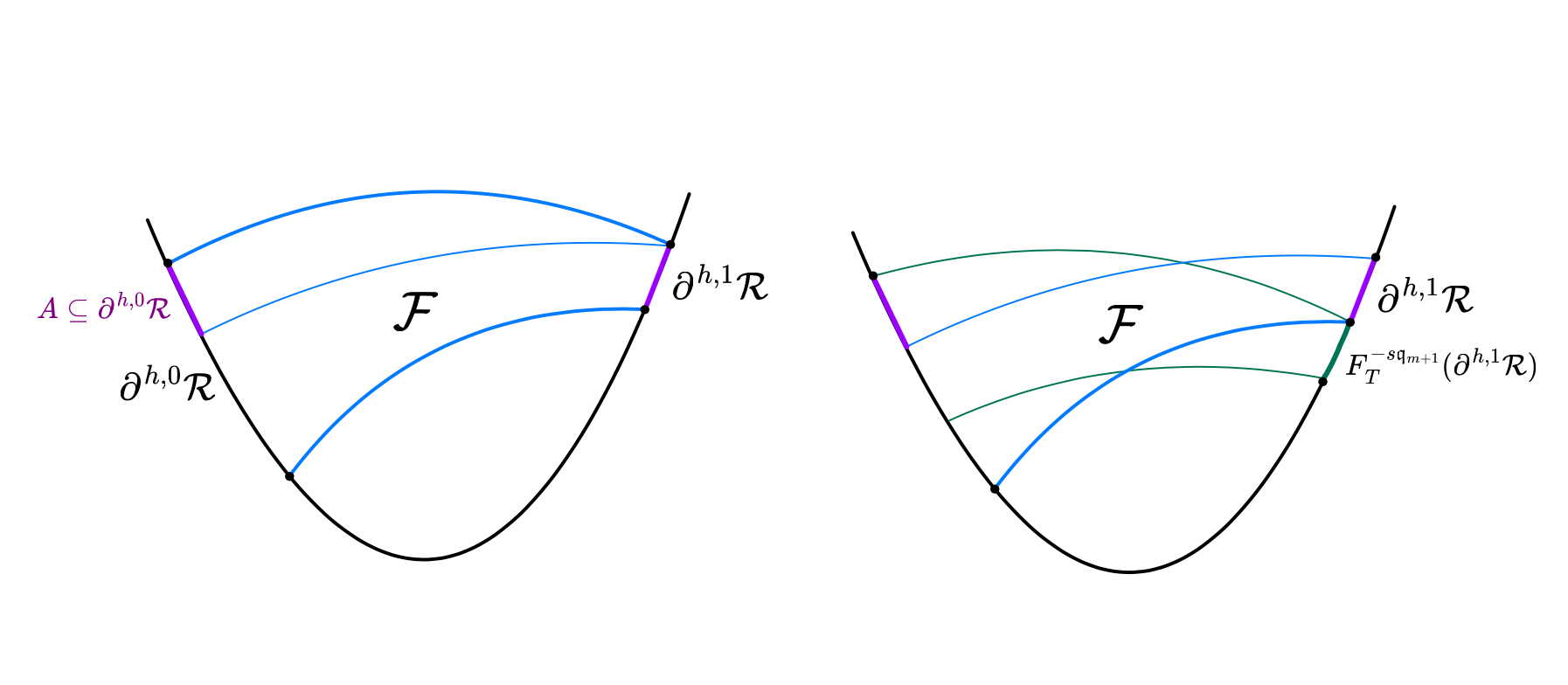
Figure 6. Illustration of the Shift Argument for Property (2a). Suppose $\displaystyle|\partial^{h,0}\mathcal{R}|>|\partial^{h,1}\mathcal{R}|$. Let $\displaystyle A\subseteq\partial^{h,0}\mathcal{R}$ be the interval indicated in the left figure with $\displaystyle|A|=|\partial^{h,1}\mathcal{R}|$. Consider any rectangle $\displaystyle\mathcal{R}^{\prime}$ in $\displaystyle V\setminus Z$ with vertical boundaries $\displaystyle\partial^{h,0}\mathcal{R}\setminus A$ and $\displaystyle\partial^{h,0}\mathcal{R}$. Then we can consecutively pull back by $\displaystyle F^{-\mathfrak{q}_{m+1}}_{T}$, and obtain a configuration on the right figure. This implies that $\displaystyle\mathcal{R}^{\prime}$ has width at most $\displaystyle 2$ by [DL3, §A.3, Lemma A.11]. Thus, by removing $\displaystyle O(1)$-buffers, we may assume Property (2a) holds.

4.2. Balanced subrectangle

It follows from the existence of the shifts (i.e., from Items (v) and (w) in the proof of Lemma 4.2) that every wide parabolic rectangle $\displaystyle\mathcal{R}$ is balanced: $\displaystyle|\partial^{h,0}\mathcal{R}^{\operatorname{new}}|=|\partial^{h,1}\mathcal{R}^{\operatorname{new}}|$ after removing $\displaystyle O(1)$ buffers; see Items (2a) and (2b) in the lemma below.

Lemma 4.2.

Let $\displaystyle\mathcal{R}$ be a wide external parabolic rectangle. Then $\displaystyle\mathcal{R}$ contains a geodesic balanced subrectangle $\displaystyle\mathcal{R}^{\operatorname{new}}$ with

$${\mathcal{W}}(\mathcal{R}^{\operatorname{new}})={\mathcal{W}}(\mathcal{R})-O(1)$$

satisfying the upper Log-Rule. More precisely, we have

1. $\displaystyle\mathcal{R}^{\operatorname{new}}$ is geodesic in $\displaystyle V-\overline{Z}$;

1. $\displaystyle|\partial^{h,0}\mathcal{R}^{\operatorname{new}}|\leq|\partial^{h,1}\mathcal{R}^{\operatorname{new}}|$;

1. $\displaystyle|\partial^{h,0}\mathcal{R}^{\operatorname{new}}|\geq|\partial^{h,1}\mathcal{R}^{\operatorname{new}}|$;

1. $\displaystyle\mathcal{R}$ obeys upper Log-Rule: $\displaystyle{\mathcal{W}}(\mathcal{R}^{\operatorname{new}})\preceq\log\frac{|\partial^{h,0}\mathcal{R}^{\operatorname{new}}|}{\operatorname{dist}(v,\partial^{h,0}\mathcal{R}^{\operatorname{new}})}+1$.

Proof.

The proof is the same as a series of lemmas (more precisely, [DL3, Lemma 4.4, Lemma 4.5, Lemma 4.10]) in [DL3, §4] and relies on shifts

• towards $\displaystyle v$ via the pullback $\displaystyle F^{-\mathfrak{q}_{m+1}}_{T}$, see (3.4) in Corollary 4.1;

• towards $\displaystyle w$ using univalent push-forward $\displaystyle F^{\mathfrak{q}_{m+1}}$, see § 3.4.1.

We remark that shifts towards $\displaystyle v$ are relatively easy, while shifts towards $\displaystyle w$ are more delicate. In general, the shift operation towards $\displaystyle w$ produces three types of curves illustrated [DL3, Figure 12]. However, when an outer protection by an external family is constructed, wide families can be shifted below the protection towards $\displaystyle w$ with uniformly bounded loss of width, see [DL3, Lemma 4.9].

Let us sketch the main steps of the proof. First, we note that by removing $\displaystyle O(1)$-buffers from $\displaystyle\mathcal{R}$, we may assume that $\displaystyle\mathcal{R}$ satisfies Property (1), (2a), (3). Indeed, Property (1) is general; see [DL3, Lemma A.5]. Property (2a) relies on the Shift Argument towards $\displaystyle v$ illustrated on Figure 6; compare with [DL3, Lemmas 4.4]. Property (3) follows from iterating (2a): we can split $\displaystyle\mathcal{R}^{\operatorname{new}}$ into at most $\displaystyle\frac{|\partial^{h,0}\mathcal{R}^{\operatorname{new}}|}{\operatorname{dist}(v,\partial^{h,0}\mathcal{R}^{\operatorname{new}})}+1$ small rectangles and use (2a) to claim that each small rectangle has width $\displaystyle\preceq 1$, see details [DL3, Lemmas 4.5].

Using shifts towards $\displaystyle w$ (push-forward, Item (w)), we can additionally impose Property (2b) (see [DL3, Lemmas 4.10]). The argument relies on extracting first an outer buffer $\displaystyle\mathcal{R}_{+}$ with width $\displaystyle\asymp 1$. Most of width of $\displaystyle\mathcal{R}$ is in $\displaystyle\mathcal{R}^{\operatorname{new}}\coloneqq\mathcal{R}\setminus\mathcal{R}_{+}$. Since curves in $\displaystyle\mathcal{R}^{\operatorname{new}}$ are protected by $\displaystyle\mathcal{R}_{+}$, the Shift Argument towards $\displaystyle w$ is applicable to and Properties (1), (2a), (3) can be claimed (together with (2b)) for $\displaystyle\mathcal{R}^{\operatorname{new}}$. ∎

Remark 4.3.

It follows from Lemma 4.2 that a rectangle $\displaystyle\mathcal{R}$, up to $\displaystyle O(1)$, can be replaced by a family $\displaystyle{\mathcal{F}}^{+}_{{\operatorname{ext}},m}(I,J)$ connecting two intervals $\displaystyle I,J$ with $\displaystyle|I|=|J|$:

$${\mathcal{W}}(\mathcal{R})=\ {\mathcal{W}}^{+}_{{\operatorname{ext}},m}(I,J)\qquad\text{where }I=\partial^{h,0}\mathcal{R}^{\operatorname{new}},J=\partial^{h,1}\mathcal{R}^{\operatorname{new}}.$$

Note that $\displaystyle\partial^{h,0}\mathcal{R},\partial^{h,0}\mathcal{R}$ can be much bigger than $\displaystyle\partial^{h,0}\mathcal{R}^{\operatorname{new}},\partial^{h,0}\mathcal{R}^{\operatorname{new}}$. We will not distinguish much between wide parabolic rectangles $\displaystyle\mathcal{R}$ and families $\displaystyle{\mathcal{F}}^{+}_{{\operatorname{ext}},m}(I,J)$. In particular, we formulate Theorem 4.4 using pairs of intervals.

4.3. Log-Rule

By the discussion in § 3.2.7, we consider a pair of intervals $\displaystyle I,J\subset T=[v,w]\in{\mathfrak{D}}_{m}$. Let us also assume that

(4.2) $$\displaystyle\text{There is an interval $\displaystyle I\subseteq T$ with }{\mathcal{W}}^{+}_{5,{\operatorname{ext}},m}(I)\geq C\gg 1.$$

We remark that if the assumption (4.2) does not hold, then we do not do any regularization of the Siegel disk on this level.

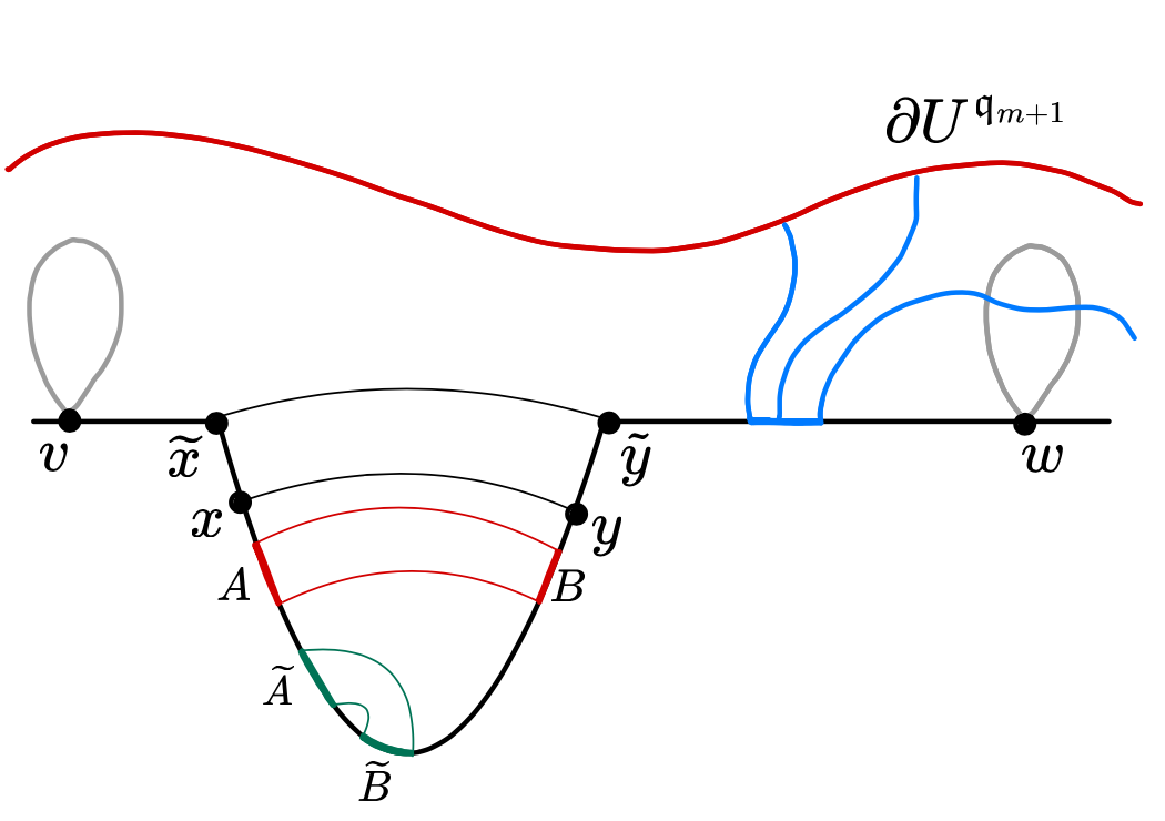
Figure 7. Illustration to the geometry of a parabolic fjord based on $\displaystyle T=[v,w]$. Wide families based on $\displaystyle[x,y]$ are external: the red rectangle between $\displaystyle A_{1},B_{1}$ represents Case (2)(i) in Theorem 4.4, while the green rectangle between $\displaystyle A_{2},B_{2}$ represents Case (2)(ii). Wide families outside of $\displaystyle[\tilde{x},\tilde{y}]$ (in blue) are either diving or vertical.

Theorem 4.4.

Under the assumption (4.2), we have the following structure in the parabolic fjords that encodes wide external families.

1. There is an outer protection: there are $\displaystyle[\widetilde{x},x],[y,\widetilde{y}]$ with

   (4.3) $$M{\mathfrak{l}}_{m+1}\coloneqq\operatorname{dist}(\widetilde{x},x)=\operatorname{dist}(\widetilde{y},y)\leq\operatorname{dist}(x,y)/100$$

   and $\displaystyle\operatorname{dist}(v,\widetilde{x})<M{\mathfrak{l}}_{m+1}/100$ such that

   $${\mathcal{W}}^{+}_{{\operatorname{ext}},m}([\widetilde{x},x],[y,\widetilde{y}])=C\gg 1.$$

2. The external families in $\displaystyle[x,y]$ satisfies the Log-Rule. More precisely,

   1. If $\displaystyle x<I<J<y$ are two intervals with

      $$\operatorname{dist}(x,I)\asymp\operatorname{dist}(J,y)\preceq|I|\asymp|J|\preceq\operatorname{dist}(I,J)$$

      and $\displaystyle|I|,|J|,\operatorname{dist}(I,J)\geq{\mathfrak{l}}_{m+1}$, then

      (4.4) $${\mathcal{W}}^{+}(I,J)-O(1)={\mathcal{W}}^{+}_{{\operatorname{ext}},m}(I,J)\asymp\log^{+}\frac{\min\{|I|,|J|\}}{\operatorname{dist}(v,I)}+1.$$

   2. If $\displaystyle x<I<J<y$ are two intervals with

      $$|\lfloor I,J\rfloor|\leq\frac{1}{2}|[x,y]|\text{ and }\min\{|I|,|J|\}\succeq\operatorname{dist}(I,J)\geq 3{\mathfrak{l}}_{m+1}$$

      and $\displaystyle|I|,|J|\geq{\mathfrak{l}}_{m+1}$, then

      (4.5) $${\mathcal{W}}^{+}(I,J)-O(1)={\mathcal{W}}^{+}_{{\operatorname{ext}},m}(I,J)\asymp\log^{+}\frac{\min\{|I|,|J|\}}{\operatorname{dist}(I,J)}+1.$$

3. For any interval $\displaystyle I\subseteq T\setminus[x,y]$, we have

   $${\mathcal{W}}^{+}_{5,{\operatorname{ext}},m}(I)=O(C)\equiv O(1).$$

4. Set

   (4.6) $$N\coloneqq\frac{\operatorname{dist}(\widetilde{y},w)}{{\mathfrak{l}}_{m+1}}.$$

   If $\displaystyle\frac{N}{\lambda M}\gg 1$, then there exists an interval $\displaystyle E\subseteq[\widetilde{y},w]$ so that

   $${\mathcal{W}}^{+}_{\lambda}(E)={\mathcal{W}}^{+,{\operatorname{ver}}}(E)+{\mathcal{W}}^{+,{\operatorname{per}}}_{\lambda,{\operatorname{div}},m}(E)+O(1)\succeq\frac{N}{\lambda M}.$$

Proof.

Justification of the theorem is the same as for [DL3, Theorem 4.1] and [DL3, Corollary 4.11].

Let $\displaystyle\mathcal{R}$ be the outermost external parabolic rectangle; see the choice of $\displaystyle S$ in [DL3, (4.15)]. By Lemma 4.2, there exists a subrectangle $\displaystyle\mathcal{R}^{\operatorname{new}}$ in $\displaystyle\mathcal{R}$ satisfying Properties (1)–(3). We set $\displaystyle[\tilde{x},x]$ and $\displaystyle[y,\tilde{y}]$ to be horizontal sides of $\displaystyle\mathcal{R}^{\operatorname{new}}$, see Figure 7. Below $\displaystyle\mathcal{R}^{\operatorname{new}}$, both left and right shifts are justified and they imply Items (1) – (3) in the same way as the proof of [DL3, Theorem 4.1].

Item (4) is relevant only if $\displaystyle N$ is much bigger than $\displaystyle M$, see (4.6) and (4.3). If this is the case, then move rectangle $\displaystyle\mathcal{R}^{\operatorname{new}}$ towards $\displaystyle w$ as shown on [DL3, Figure 14]; the result is a numerous (i.e., $\displaystyle\asymp N/M$) collection of families emerging from $\displaystyle[\tilde{y},w]$. Only $\displaystyle O(1)$ curves in this collection are external because of the outermost choice of $\displaystyle\mathcal{R}$. By selecting $\displaystyle E$ well inside (in terms of $\displaystyle\lambda$) $\displaystyle[\tilde{y},w]$, we justify Item (4). ∎

4.4. Central rectangles

As in [DL3, §4.5], we say that a parabolic rectangle $\displaystyle\mathcal{R}$ based on $\displaystyle T^{\prime}$ is central if

(4.7) $$0.9<\frac{\operatorname{dist}_{T}(v,\lfloor\partial^{h}\mathcal{R}\rfloor)}{\operatorname{dist}_{T}(\lfloor\partial^{h}\mathcal{R}\rfloor,w)}<1.1;$$

i.e. if the distances from $\displaystyle\partial^{h}\mathcal{R}$ to $\displaystyle v$ and $\displaystyle w$ are essentially the same.

Consider a sufficiently big $\displaystyle K\gg 1$ that dominates $\displaystyle O(1)$ in (4.4) but with $\displaystyle\log\frac{\operatorname{dist}(x,y)}{M{\mathfrak{l}}_{m+1}}\gg K$. Then we can split the interval $\displaystyle[x,y]$ as a concatenation

(4.8) $$[x,y]=A\cup Q\cup B,\qquad\text{with $\displaystyle|A|=|B|$ and}\ {\mathcal{W}}^{+}(A,B)=K.$$

We say that the interval $\displaystyle Q$ and the associated fjord $\displaystyle{\mathfrak{F}}(Q)$ (see §3.3.1) are obtained by submerging into depth $\displaystyle K$.

Lemma 4.5 (Essentially [DL3, Lemma 4.12]).

Let us fix any $\displaystyle K\gg L\gg 1$. We claim that there are three possibilities,

1. the interval $\displaystyle[x,y]$ does not support external families of width $\displaystyle\geq K$ with combinatorial separation: there are no $\displaystyle I,J\subset[x,y]$ such that

   $${\mathcal{W}}^{+}(I,J)\geq K,\hskip 28.45274pt\text{ and }\ |I|=|J|\leq\frac{1}{2}\operatorname{dist}(I,J).$$

   If this possibility occurs, then we have $\displaystyle\log\frac{\operatorname{dist}(x,y)}{M{\mathfrak{l}}_{m+1}}\preceq K$.

Conversely, if $\displaystyle\log\frac{\operatorname{dist}(x,y)}{M{\mathfrak{l}}_{m+1}}\gg K$, then we have another two possibilities:

1. by submerging into depth $\displaystyle K$ as in (4.8), we obtain a balanced central geodesic rectangle with width $\displaystyle L$; namely: there is a decomposition $\displaystyle[x,y]=A\cup I\cup P\cup J\cup B$ into concatenation of intervals such that

   $${\mathcal{W}}^{+}(A,B)=K,\qquad|A|=|B|,$$

   $${\mathcal{W}}^{+}(I,J)=L,\qquad|I|=|J|,$$

   $$|P|\geq 6(|A|+|I|+|J|+|B|)=12(|A|+|I|),$$

   and geodesic rectangle $\displaystyle\mathcal{R}=\mathcal{R}(I,J)$ connecting $\displaystyle I$ and $\displaystyle J$ is central (4.7);

2. there exists an interval $\displaystyle E$ with the exponential boost (see §4.6.2):

   $$\log\left({\mathcal{W}}^{+,{\operatorname{ver}}}(E)+{\mathcal{W}}^{+,{\operatorname{per}}}_{\lambda,{\operatorname{div}},m}(E)\right)\succeq K-\log(\lambda).$$

Proof.

Suppose case (a) does not occur. If $\displaystyle\log\frac{N}{M}\leq K$, then the interval

$$I=[x+e^{K}M{\mathfrak{l}}_{m+1},x+e^{K+L}M{\mathfrak{l}}_{m+1}]{\ \ }\text{ and }{\ \ }J=[y-e^{K+L}M{\mathfrak{l}}_{m+1},y-e^{K}M{\mathfrak{l}}_{m+1}]$$

are balanced central intervals, and the corresponding geodesic rectangle has width $\displaystyle L+O(1)$ by Theorem 4.4 (Log-Rule), Claim (2). Therefore, we are in case (b).

On the other hand, if $\displaystyle\log\frac{N}{M}\geq K$, then applying the $\displaystyle\log$ to the main estimate in Claim (4) of Theorem 4.4, we obtain

$$\qquad\log\left({\mathcal{W}}^{+,{\operatorname{ver}}}(E)+{\mathcal{W}}^{+,{\operatorname{per}}}_{\lambda,{\operatorname{div}},m}(E)\right)\geq\log\left(\frac{N}{\lambda M}\right)-O(1)\ \succeq\\ \log\left(\frac{N}{M}\right)-O(\log\lambda)\geq K-O(\log(\lambda)),\qquad$$

and we are in case (c). ∎

4.5. Bistable part $\displaystyle\Xi^{k}_{T}$ under protection

It follows immediately from the Log-Rule that the Fjord obtained by submerging into depth $\displaystyle K$ has large stability.

Lemma 4.6 ($\displaystyle\mathfrak{F}(Q))\subset\Xi^{k}_{T}$).

There is an exponent $\displaystyle a>1$ with the following property. If $\displaystyle K\gg 1$ is sufficiently big, then the Fjord $\displaystyle\mathfrak{F}(Q))$ obtained by submerging into depth $\displaystyle K$ as in (4.8) is within bistable part $\displaystyle\Xi^{k}_{T}$ of the fjord $\displaystyle\mathfrak{F}(T)$ (see §3.3.4), where $\displaystyle k=\lfloor a^{K}\rfloor$.

Proof.

We select $\displaystyle a>1$ to be sufficiently small depending on the comparison ``$\displaystyle\asymp$'' in the Log-Rule of Theorem 4.4 and assume that $\displaystyle K\gg 1$ is sufficiently big to dominate $\displaystyle O(1)$ in (4.4). Then the family $\displaystyle{\mathcal{F}}^{+}(I,J)$ representing $\displaystyle{\mathcal{W}}^{+}(I,J)$ in (4.8) contains a geodesic rectangle $\displaystyle\mathcal{R}$ with width $\displaystyle K-O(1)$.

Divide the rectangle $\displaystyle\mathcal{R}$ into four rectangles $\displaystyle\mathcal{R}^{i},i=1,2,3,4$, with

$${\mathcal{W}}(\mathcal{R}^{1})=K-O(1)\quad\text{ and }{\mathcal{W}}(\mathcal{R}^{2}),{\mathcal{W}}(\mathcal{R}^{3}),{\mathcal{W}}(\mathcal{R}^{4})\geq 5$$

so that $\displaystyle\mathcal{R}^{i+1}$ is nested inside of $\displaystyle\mathcal{R}^{i}$, $\displaystyle i=1,2,3$. We assume that $\displaystyle\mathcal{R}^{i}$ has horizontal boundary $\displaystyle I^{i},J^{i}$. By the Log-Rule and potentially making $\displaystyle a$ smaller, we have that $\displaystyle|I^{2}|,|J^{2}|\geq(a+\varepsilon)^{K-O(1)}\geq 2k$.

Let $\displaystyle\mathcal{R}(I^{i},J^{i}),i=3,4$ be the geodesic rectangle in $\displaystyle V\setminus\overline{Z}$ connecting $\displaystyle I^{i}$ and $\displaystyle J^{i}$. Then $\displaystyle{\mathcal{W}}(\mathcal{R}(I^{i},J^{i}))\geq{\mathcal{W}}(\mathcal{R}^{i})-1\geq 4$ (see [DL3, Lemma A.5]). Since $\displaystyle|I^{2}|,|J^{2}|\geq 2k$ $\displaystyle\mathcal{R}(I^{i},J^{i})\subseteq\mathfrak{F}^{2k}_{\text{stab}}(T)$ for $\displaystyle i=3,4$.

Suppose for contradiction that $\displaystyle{\mathfrak{F}}(Q)\not\subset\Xi^{k}_{T}=F^{-k\mathfrak{q}_{m+1}}_{T}(\mathfrak{F}^{2k}_{\text{stab}}(T))$. Then the pullback $\displaystyle F^{-k\mathfrak{q}_{m+1}}_{T}(\mathcal{R}(I^{3},J^{3}))$ must cross $\displaystyle\mathcal{R}(I^{4},J^{4})$. This is not possible as wide rectangles cannot cross. ∎

4.6. Welding of $\displaystyle{\widehat{Z}}^{m+1}$ and parabolic fjords into $\displaystyle{\widehat{Z}}^{m}$

As in [DL3, § 5.1.9], we say that a regularization $\displaystyle{\widehat{Z}}^{m}={\widehat{Z}}^{m+1}\cup\bigcup_{I}\widehat{\mathfrak{F}}_{I}$ is within $\displaystyle\operatorname{orb}_{-\mathfrak{q}_{m+1}+1}\mathcal{R}$ if all relevant objects are within the backward orbit of a rectangle $\displaystyle\mathcal{R}$. In particular, we require that $\displaystyle\beta_{I}$ together with protection $\displaystyle A_{I}\setminus{\widehat{Z}}^{m+1}$ and extra protection $\displaystyle\mathcal{X}_{I}$ are in $\displaystyle\mathcal{R}$. Then $\displaystyle{\widehat{Z}}^{m}$ is obtained from $\displaystyle{\widehat{Z}}^{m+1}$ by spreading around the parabolic fjord $\displaystyle\widehat{\mathfrak{F}}_{I}$ below $\displaystyle\beta_{I}$.

The following regularization is a restatement of [DL3, Corollary 7.3] with simplified notations. The proof is the same: it is non-dynamical and relies only on the [DL3, Welding Lemma 7.1], which itself relies only on the Log-Rule in $\displaystyle{\widehat{Z}}^{m+1}$ and in parabolic fjords. For convenience, we comment on how the Welding Lemma implies the regularization $\displaystyle{\widehat{Z}}^{m+1}\leadsto{\widehat{Z}}^{m}$ in §4.6.1.

Theorem 4.7 (Regularization $\displaystyle{\widehat{Z}}^{m+1}\leadsto{\widehat{Z}}^{m}$).

Let $\displaystyle\mathcal{R}$ be an external parabolic rectangle based on $\displaystyle T^{\prime}$ with $\displaystyle{\mathcal{W}}(\mathcal{R})\gg 1$. Let $\displaystyle{\widehat{Z}}^{m+1}$ be a geodesic pseudo-Siegel disk. Then:

1. either there is a geodesic pseudo-Siegel disk $\displaystyle{\widehat{Z}}^{m}={\widehat{Z}}^{m+1}\cup\bigcup_{I}\widehat{\mathfrak{F}}_{I}$ with its level-$\displaystyle m$ regularization within $\displaystyle\operatorname{orb}_{-\mathfrak{q}_{m+1}+1}\mathcal{R}$;

2. or there is an interval

   $$\qquad\quad I\subset T^{\prime},{\ \ }{\ \ }|I|>{\mathfrak{l}}_{m+1}{\ \ }{\ \ }\text{such that}{\ \ }{\ \ }\\ \log\Big({\mathcal{W}}^{+,{\operatorname{ver}}}(I)+{\mathcal{W}}^{+,{\operatorname{per}}}_{\lambda,{\operatorname{div}},m}(I)\Big)\succeq{\mathcal{W}}(\mathcal{R});\qquad\qquad$$

3. or there is a grounded rel $\displaystyle{\widehat{Z}}^{m+1}$ interval

   $$I\subset\partial Z{\ \ }{\ \ }\text{ with }{\ \ }|I|\leq{\mathfrak{l}}_{m+1}{\ \ }\text{ such that }{\ \ }\log{\mathcal{W}}^{+}_{\lambda}(I)\succeq{\mathcal{W}}(\mathcal{R}).$$

Remark 4.8 (Parameter $\displaystyle{\boldsymbol{\delta}}$).

We remark that Theorem 4.7 implicitly fixes a parameter $\displaystyle{\boldsymbol{\delta}}$, see [DL3, Remark 7.5]; this is a key parameter controlling the non-invariance of $\displaystyle{\widehat{Z}}^{m}$ see [DL3, Assumption 2 in §5.1]. To simplify the exposition, an explicit reference to $\displaystyle{\boldsymbol{\delta}}$ is omitted in this paper.

4.6.1. Comments to Theorem 4.7

As we have already mentioned, [DL3, Welding Lemma 7.1] relies only on the Log-Rule in $\displaystyle{\widehat{Z}}^{m+1}$ and in parabolic fjords in the form of (4.5); therefore, as a consequence of Theorem 4.4, the Welding Lemma is also applicable in our case of $\displaystyle\psi^{\bullet}$-ql maps. It ultimately implies a fundamental property of $\displaystyle{\widehat{Z}}^{m}$ that annuli $\displaystyle A_{I}$ have positive moduli: $\displaystyle\operatorname{mod}(A_{I})\geq\delta$; see [DL3, Assumption 2 in §5]. Theorem 4.7 follows from the Welding Lemma by implementing the following steps, as in [DL3, §7.2]:

1. First, we can remove $\displaystyle\asymp 1$ outer buffer from $\displaystyle\mathcal{R}$ to obtain $\displaystyle\mathcal{R}^{\operatorname{new}}$ and claim Log-Rule below the buffer by Theorem 4.4. In particular, the $\displaystyle\mathcal{R}^{\operatorname{new}}$ obeys the Log-Rule stated in (4.4).

2. We further remove from $\displaystyle\mathcal{R}^{\operatorname{new}}$ outer-buffer with width $\displaystyle\frac{1}{2}{\mathcal{W}}(\mathcal{R}^{\operatorname{new}})$. If $\displaystyle\mathcal{R}^{\operatorname{New}}$ is not central, then Case 2 occurs by Lemma 4.5, where $\displaystyle I\coloneqq E$.

3. By the Welding Lemma (as in [DL3, Lemma 7.1]), either we have regularization $\displaystyle{\widehat{Z}}^{m}=Z^{m}\cup{\widehat{Z}}^{m+1}$ by constructing dams and protecting annuli in $\displaystyle\mathcal{R}^{\operatorname{New}}$, and thus in Case 1, or we have Case 3.

4.6.2. Exponential Boosts

We refer to Case (c) of Lemma 4.5 and to Cases (2), (3) of Theorem 4.7 as Exponential Boosts. Roughly, if a pathology in one of these cases occurs, then the Log-Rule implies an exponential amplification of the degeneration.

5. Covering and Lair lemmas

In this section, we state Amplification Theorem 5.1, a modification of [DL3, Amplification Theorem 8.1]. The main difference is that the degeneration for $\displaystyle\psi^{\bullet}$-maps can be vertical; this leads to Alternative (ii) in Theorem 5.1.

Amplification is achieved in two steps: spreading around using the Covering Lemma, followed by the Snake-Lair Lemma to detect a large amount of submergence and amplify the degeneration at a deeper level. The Covering Lemma step is stated as Lemma 5.2; it is almost the same as for quadratic polynomials and relies on push-forwards that were discussed in §3.4, §3.6.1.

The Snake Lemma step is stated as Lemma 5.3, where Alternative (ii) is new compared to the case of quadratic polynomials. The strategy of the proof is to show if (ii) does not hold, then most degenerations are non-vertical, and we can reduce to the same argument as in the quadratic polynomial case.

Let $\displaystyle F=(f,\iota)\colon{\ \ }(U,\overline{Z}_{U})\rightrightarrows(V,\overline{Z})$ be $\displaystyle\psi^{\bullet}$-ql Siegel map with rotation number $\displaystyle\theta_{0}$. Recall that the width of $\displaystyle F$ is

$$K_{F}={\mathcal{W}}^{\bullet}(F)\coloneqq{\mathcal{W}}(V\setminus\overline{Z}).$$

Amplification Theorem 5.1.

There are increasing functions

$${\boldsymbol{\lambda}}_{\mathbf{t}},{\ \ }{\mathbf{K}}_{\mathbf{t}}{\ \ }{\ \ }\text{ for }\mathfrak{t}>1{\ \ }{\ \ }\text{ with }{\ \ }{\boldsymbol{\lambda}}_{\mathbf{t}},\ {\mathbf{K}}_{\mathbf{t}}\ \underset{t\to\infty}{\longrightarrow}\ +\infty$$

such that the following holds. Suppose that there is a combinatorial interval

$$I\subset\partial Z{\ \ }{\ \ }\text{ such that }{\ \ }{\mathcal{W}}^{+}_{{\boldsymbol{\lambda}}_{\mathbf{t}}}(I)\eqqcolon K\geq{\mathbf{K}}_{\mathbf{t}}{\ \ }\text{ and }{\ \ }|I|\leq|\theta_{0}|/(2{\boldsymbol{\lambda}}_{\mathbf{t}}).$$

Consider a geodesic pseudo-Siegel disk $\displaystyle{\widehat{Z}}^{m}$, where $\displaystyle m$ is the level of $\displaystyle I$. Then

1. either there is a grounded rel $\displaystyle{\widehat{Z}}^{m}$ interval

   $$J\subset\partial Z{\ \ }{\ \ }\text{ such that }{\ \ }{\mathcal{W}}^{+}_{{\boldsymbol{\lambda}}_{\mathbf{t}}}(J)\geq{\mathbf{t}}K{\ \ }\text{ and }{\ \ }|J|\leq|I|.$$

2. or $\displaystyle K_{F}\succeq_{{\boldsymbol{\lambda}}_{\mathbf{t}}}K\mathfrak{q}_{m+1}$.

Proof.

As in [DL3, §8], the proof follows from Lemma 5.2 (application of the Covering Lemma) followed by Snake-Lair Lemma 5.3.

For convenience, as in [DL3, end of §8.2], we can assume that one of the endpoints of $\displaystyle I$ is in $\displaystyle{\operatorname{CP}}_{m}$. Indeed, we cover $\displaystyle I$ with two combinatorial intervals $\displaystyle I_{a}\cup I_{b}\supset I$ satisfying such a property and observe that $\displaystyle{\mathcal{W}}^{+}_{{\boldsymbol{\lambda}}_{\mathbf{t}}}(I)=K$ implies that either

(5.1) $${\mathcal{W}}^{+}_{{\boldsymbol{\lambda}}_{\mathbf{t}}-1}(I_{a})\geq K/2\qquad\text{ or }\qquad{\mathcal{W}}^{+}_{{\boldsymbol{\lambda}}_{\mathbf{t}}-1}(I_{b})\geq K/2$$

holds. ∎

5.1. Applying the Covering Lemma

We will denote by $\displaystyle I^{m}$ the projection of a regular interval $\displaystyle I\subset\partial Z$ onto $\displaystyle\partial{\widehat{Z}}^{m}$. The same argument as in [DL3, Lemma 8.2] allows us to apply the Covering Lemma (see [KL1] or [DL3, Lemma 8.5]) and obtain the following theorem for $\displaystyle\psi^{\bullet}$-maps. See §3.4.2, §3.4.3,  §3.6.1 and Figure 5 for the preparation to apply the covering lemma.

Lemma 5.2.

For every $\displaystyle{\boldsymbol{\kappa}}>1$ and $\displaystyle\lambda>10$, there is $\displaystyle{\mathbf{K}}_{\lambda,{\boldsymbol{\kappa}}}>1$ and $\displaystyle C_{\boldsymbol{\kappa}}$ (independent of $\displaystyle\lambda$) such that the following holds. Suppose that there is a combinatorial interval

$$I\subset\partial Z{\ \ }{\ \ }\text{ such that }{\ \ }{\mathcal{W}}^{+}_{\lambda+2}(I)=K\geq{\mathbf{K}}_{\lambda,{\boldsymbol{\kappa}}},{\ \ }{\ \ }|I|\leq|\theta_{0}|/(2\lambda+4),{\ \ }{\ \ }m=\operatorname{Level}(I)$$

and such that one of the endpoints of $\displaystyle I$ is in $\displaystyle{\operatorname{CP}}_{m}$. Let $\displaystyle{\widehat{Z}}^{m}$ be a geodesic pseudo-Siegel disk, and

$$I_{s}\subset\partial Z,{\ \ }{\ \ }I_{s}=f^{i_{s}}(I),{\ \ }{\ \ }s\in\{0,1,\dots,\mathfrak{q}_{m+1}-1\}$$

be the intervals obtained by spreading around $\displaystyle I=I_{0}$ (see [DL3, §2.1.5]). Then every interval $\displaystyle I_{s}$ is well-grounded rel $\displaystyle{\widehat{Z}}^{m}$ and its projection $\displaystyle I^{m}_{s}\subset\partial{\widehat{Z}}^{m}$ is

1. either $\displaystyle[{\boldsymbol{\kappa}}K,10]$-wide: $\displaystyle{\mathcal{W}}_{10}(I^{m}_{s})\geq{\boldsymbol{\kappa}}K$

2. or $\displaystyle[C_{{\boldsymbol{\kappa}}}K,\lambda]$-wide: $\displaystyle{\mathcal{W}}_{\lambda}(I^{m}_{s})\geq C_{{\boldsymbol{\kappa}}}K$

5.2. Lair of snakes

For our convenience, we enumerate intervals clockwise in the following lemma. We remark that the Snake-Lair lemma for $\displaystyle\psi^{\bullet}$-maps needs to be modified. In particular, we have Alternative (ii) in the conclusion (c.f. [DL3, Lemma 8.6]).

Snake-Lair Lemma 5.3.

For every $\displaystyle{\mathbf{t}}>2$ there are $\displaystyle{\boldsymbol{\kappa}},{\boldsymbol{\lambda}},{\mathbf{K}}\gg_{{\boldsymbol{\delta}}}1$ such that the following holds. Suppose that $\displaystyle{\widehat{Z}}^{m}$ is a pseudo-Siegel disk with $\displaystyle{\mathfrak{l}}_{m}<{\boldsymbol{\lambda}}/4$. Let

$$I_{n+1}=I_{0},I_{1},\dots,I_{n}\subset\partial{\widehat{Z}}^{m},{\ \ }{\ \ }{\ \ }|I_{k}|={\mathfrak{l}}_{m},{\ \ }\operatorname{dist}(I_{k},I_{k+1})\leq{\mathfrak{l}}_{m}$$

be a sequence of well-grounded intervals enumerated clockwise such that every $\displaystyle I_{s}$ is one of the following two types

1. either $\displaystyle I_{s}$ is $\displaystyle[{\boldsymbol{\kappa}}K,10]$-wide,

2. or $\displaystyle I_{s}$ is $\displaystyle[C_{{\boldsymbol{\kappa}}}K,{\boldsymbol{\lambda}}]$-wide,

where $\displaystyle K\geq{\mathbf{K}}$ and $\displaystyle C_{\boldsymbol{\kappa}}$ is a constant (from Lemma 5.2) independent of $\displaystyle{\boldsymbol{\lambda}}$. Then

1. either there is a grounded rel $\displaystyle{\widehat{Z}}^{m}$ interval

   $$J\subset\partial Z{\ \ }{\ \ }\text{ such that }{\ \ }{\mathcal{W}}^{+}_{{\boldsymbol{\lambda}}_{\mathbf{t}}}(J)\geq{\mathbf{t}}K{\ \ }\text{ and }{\ \ }|J|\leq|I|.$$

2. or $\displaystyle K_{F}\succeq_{\boldsymbol{\lambda}}K\mathfrak{q}_{m+1}$.

The proof below follows the strategy of [DL3, Lemma 8.6]. In the case of quadratic polynomials, degeneration can not go to infinity [DL3, Lemma 6.14]. Claim 1 is a substitution for [DL3, Lemma 6.14]: if Alternative (ii) does not hold, then there is a long sequence of intervals from where the degeneration does not go to the outer boundary $\displaystyle\partial V$. With respect to the notion of ``relatively peripheral'' curves, Items 1 and 2 of Lemma 5.3 take a form similar to that in [DL3, Lemma 8.6], see Claim 2 below. After Claim 2, the proof is similar to the case of quadratic polynomials.

Proof.

Let us assume that the alternative (ii) of Lemma 5.3 does not hold. We will show that the alternative (i) of Lemma 5.3 must hold.

Let us enlarge every $\displaystyle I_{i}$ into a well-grounded interval $\displaystyle{\widehat{I}}_{i}\subset\partial{\widehat{Z}}^{m}$ by adding to $\displaystyle I_{i}$ the interval between $\displaystyle I_{i}$ and $\displaystyle I_{i+1}$ if $\displaystyle I_{i}$ and $\displaystyle I_{i+1}$ are disjoint. Since the distances between the $\displaystyle I_{i}$ and $\displaystyle I_{i+1}$ are $\displaystyle\leq{\mathfrak{l}}_{m}$, we have $\displaystyle|{\widehat{I}}_{i}|\leq 2{\mathfrak{l}}_{m}$.

Let $\displaystyle\mathcal{I}$ consist of all intervals $\displaystyle{\widehat{I}}_{i}$ so that $\displaystyle{\mathcal{W}}^{+,ver}({\widehat{I}}_{i})\geq\frac{K}{{\boldsymbol{\lambda}}^{3}}$. Suppose $\displaystyle\#\mathcal{I}\geq\frac{n}{{\boldsymbol{\lambda}}}$. Since $\displaystyle n\asymp\mathfrak{q}_{m+1}$, we have

$$K_{F}\succeq\frac{K}{{\boldsymbol{\lambda}}^{4}}\mathfrak{q}_{m+1}.$$

Therefore, the alternative (ii) of Lemma 5.3 holds. Thus, we may assume that $\displaystyle\#\mathcal{I}\leq\frac{n}{{\boldsymbol{\lambda}}}$, i.e., not a lot of intervals have large vertical degenerations.

Let us assume that $\displaystyle\#\mathcal{I}\geq 2$. The case $\displaystyle\#\mathcal{I}=1$ can be treated similarly by allowing $\displaystyle{\widehat{I}}_{k}={\widehat{I}}_{k+l}$ in Claim 1 below. The case $\displaystyle\#\mathcal{I}=0$ is essentially the case of quadratic polynomials – the outer boundary $\displaystyle\partial V$ is well separated from $\displaystyle{\widehat{Z}}^{m}$.

Claim 1 (Substitution of [DL3, Lemma 6.14]; see Figure 9).

There is a sub-sequence

(5.2) $${\widehat{I}}_{k},{\widehat{I}}_{k+1},\dots,{\widehat{I}}_{k+l}\subset\partial{\widehat{Z}}^{m},{\ \ }{\ \ }{\ \ }|{\widehat{I}}|\leq 2{\mathfrak{l}}_{m}$$

such that

1. $\displaystyle l\geq{\boldsymbol{\lambda}}/2$,

2. $\displaystyle{\mathcal{W}}^{+,ver}({\widehat{I}}_{k}),{\mathcal{W}}^{+,ver}({\widehat{I}}_{k+l})\geq\frac{K}{{\boldsymbol{\lambda}}^{3}}$,

3. $\displaystyle{\mathcal{W}}^{+,ver}({\widehat{I}}_{j})\leq\frac{K}{{\boldsymbol{\lambda}}^{3}}$ for all $\displaystyle k<j<k+l$.

Proof.

This claim follows from $\displaystyle 2\leq\#\mathcal{I}\leq\frac{n}{{\boldsymbol{\lambda}}}$. ∎

Let $\displaystyle L=\lfloor{\widehat{I}}_{k+1},{\widehat{I}}_{k+l-1}\rfloor$. Let $\displaystyle I\subseteq L$. We say an arc $\displaystyle\alpha\in\mathcal{F}_{\lambda}(I)$ is relatively peripheral with respect to $\displaystyle L$ if it is either peripheral, or it is vertical and the last time $\displaystyle\alpha$ intersects $\displaystyle{\widehat{Z}}^{m}$ is outside of $\displaystyle L$. We denote by $\displaystyle{\mathcal{W}}^{per/L}_{\lambda}(I)$ the extremal width of relatively peripheral arcs. Since relatively peripheral arc outside of $\displaystyle{\widehat{Z}}^{m}$ is in fact peripheral, we have

$${\mathcal{W}}^{+,per/L}_{\lambda}(I)={\mathcal{W}}^{+,per}_{\lambda}(I).$$

Let us also denote by $\displaystyle\mathcal{R}_{k}$ and $\displaystyle\mathcal{R}_{k+l}$ the rectangles connecting $\displaystyle I_{k}$ and $\displaystyle\partial V$ with width $\displaystyle{\mathcal{W}}(\mathcal{R}_{k}),{\mathcal{W}}(\mathcal{R}_{k+l})\succeq\frac{K}{{\boldsymbol{\lambda}}^{3}}$.

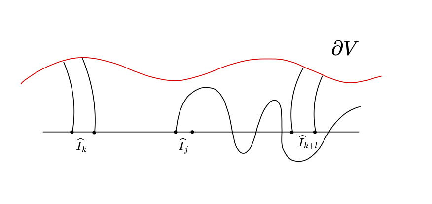
Figure 9. Illustration to the intervals $\displaystyle\widehat{I}_{j}$ from Claim 1 and to families emerging from the $\displaystyle\widehat{I}_{J}$.

Claim 2 (c.f. [DL3, (1) and (2) of Lemma 8.6]).

For any $\displaystyle k<i<k+l$, we have that $\displaystyle{\widehat{I}}_{i}$ is one of the following two types

1. either $\displaystyle{\mathcal{W}}^{per/L}_{10}({\widehat{I}}_{i})\geq{\boldsymbol{\kappa}}K/2$,

2. or $\displaystyle{\mathcal{W}}^{per/L}_{{\boldsymbol{\lambda}}}({\widehat{I}}_{i})\geq C_{\boldsymbol{\kappa}}K/2$

Proof.

By Claim 1, $\displaystyle{\mathcal{W}}^{+,ver}({\widehat{I}}_{j})\leq\frac{K}{{\boldsymbol{\lambda}}^{3}}$ for all $\displaystyle k<j<k+l$. Therefore, the non relatively peripheral degeneration

$${\mathcal{W}}_{{\boldsymbol{\lambda}}}({\widehat{I}}_{i})-{\mathcal{W}}^{per/L}_{{\boldsymbol{\lambda}}}({\widehat{I}}_{i})\leq{\boldsymbol{\lambda}}\frac{K}{{\boldsymbol{\lambda}}^{3}}=\frac{K}{{\boldsymbol{\lambda}}^{2}},\text{ and }$$

$${\mathcal{W}}_{10}({\widehat{I}}_{i})-{\mathcal{W}}^{per/L}_{10}({\widehat{I}}_{i})\leq 10\frac{K}{{\boldsymbol{\lambda}}^{3}}=\frac{10K}{{\boldsymbol{\lambda}}^{3}}.$$

Since $\displaystyle 1/{\boldsymbol{\lambda}}\ll 1$, the claim follows. ∎

Claim 3.

(c.f. Claim 1 in [DL3, §8.2]) Let $\displaystyle k+20<i<k+l-20$. Lemma 5.3 holds if there is a Type (I) interval $\displaystyle{\widehat{I}}_{i}$ such that

$${\mathcal{W}}^{per/L}_{10}({\widehat{I}}_{i})-{\mathcal{W}}^{+,per}_{10}({\widehat{I}}_{i})\geq{\boldsymbol{\kappa}}K/4.$$

Proof.

Since $\displaystyle k+20<i<k+l-20$, we conclude that $\displaystyle 10{\widehat{I}}_{i}\subseteq L$. Thus, $\displaystyle{\mathcal{W}}^{per/L}_{10}({\widehat{I}}_{i})={\mathcal{W}}^{per}_{10}({\widehat{I}}_{i})$. Therefore, the claim follows immediately from [DL3, Lemma 6.8]. ∎

Therefore, we may assume that any Type (I) interval $\displaystyle{\widehat{I}}_{i}$ for $\displaystyle k+20<i<k+l-20$ satisfies

$${\mathcal{W}}^{+,per}_{10}({\widehat{I}}_{i})\geq{\boldsymbol{\kappa}}K/4.$$

Claim 4.

(c.f. Claim 2 in [DL3, §8.2]) There is a sub-sequence

(5.3) $${\widehat{I}}_{i},{\widehat{I}}_{i+1},\dots,{\widehat{I}}_{i+{\boldsymbol{\lambda}}/20}\subset\partial{\widehat{Z}}^{m},$$

such that $\displaystyle[i,i+{\boldsymbol{\lambda}}/20]\subseteq[k+20,k+l-20]$, and for every interval $\displaystyle{\widehat{I}}_{j}$ in (5.3), we have $\displaystyle{\mathcal{W}}^{+,{\operatorname{per}}}_{{\boldsymbol{\lambda}}/4}({\widehat{I}}_{j})\leq 5$.

Proof.

Suppose for contradiction that $\displaystyle({\widehat{I}}_{j})$ has a sub-sequence $\displaystyle(L_{j}),j=0,...,t$ with

• $\displaystyle L_{0}={\widehat{I}}_{k}$, $\displaystyle L_{t}={\widehat{I}}_{k+l}$, and

• $\displaystyle L_{j}={\widehat{I}}_{\ell(j)}$ such that $\displaystyle\ell(j)<\ell(j+1)\leq\ell(j)+{\boldsymbol{\lambda}}/10$, and

• $\displaystyle{\mathcal{W}}_{{\boldsymbol{\lambda}}/4}^{+,per}(L_{j})\geq 5$ for $\displaystyle j=1,...,t-1$.

Since $\displaystyle{\mathcal{W}}(\mathcal{R}_{k}),{\mathcal{W}}(\mathcal{R}_{k+l})\succeq\frac{K}{{\boldsymbol{\lambda}}^{3}}\geq 5$, most of the curves in $\displaystyle\mathcal{F}^{+,per}_{{\boldsymbol{\lambda}}/4}({\widehat{I}}_{j})$ do not cross the rectangles $\displaystyle\mathcal{R}_{k}$ and $\displaystyle\mathcal{R}_{k+l}$. Thus, by [DL3, Lemma 6.14], such families $\displaystyle\mathcal{F}^{+,per}_{{\boldsymbol{\lambda}}/4}({\widehat{I}}_{j}),j=1,...,t-1$ would block each other, which is a contradiction and the claim follows. ∎

Claim 5.

(c.f. Claim 3 in [DL3, §8.2]) There is $\displaystyle\mathbf{k}$ depending on $\displaystyle\mathbf{t}$ and $\displaystyle{\boldsymbol{\kappa}}$ but not on $\displaystyle{\boldsymbol{\lambda}}$ such that the alternative (i) of Lemma 5.3 holds if there are $\displaystyle\mathbf{k}$ consecutive Type ((I)) intervals in (5.3)

Proof.

Suppose that there are $\displaystyle\mathbf{k}$ consecutive intervals of Type ((I)), denoted by $\displaystyle{\widehat{I}}_{a},...,{\widehat{I}}_{b}$ with $\displaystyle b-a=\mathbf{k}-1$. Denote by

$$I_{a,b}\coloneqq\lfloor{\widehat{I}}_{a},{\widehat{I}}_{b}\rfloor,\text{ and }J_{a,b}\coloneqq\bigcap_{i=a}^{b}(\frac{{\boldsymbol{\lambda}}}{4}{\widehat{I}}_{i})^{c}.$$

Then we have $\displaystyle W^{+}(I_{a,b},J_{a,b})=O(\mathbf{k})$ by Claim 4. Since families $\displaystyle\mathcal{F}^{+,per}_{10}({\widehat{I}}_{i})$ have small overlaps (they block each other), by Claim 3, there is a rectangle

$$\mathcal{R}\subseteq\bigcup_{i=a}^{b}\mathcal{F}^{+,per}_{10}({\widehat{I}}_{i})\text{ with }{\mathcal{W}}(\mathcal{R})\succeq\mathbf{k}{\boldsymbol{\kappa}}K.$$

The proof now proceeds exactly the same as the proof of Claim 3 in [DL3, §8.2]. ∎

We now assume that among $\displaystyle\mathbf{k}$ consecutive intervals in (5.3), there is at least one Type ((II)) interval. Now we can perform the similar construction as in the quadratic polynomial case, and enumerate Type ((II)) intervals in (5.3) as

$${\widehat{I}}_{i_{0}},...,{\widehat{I}}_{i_{s}},i_{j}<i_{j+1}<i_{j}+\mathbf{k},$$

where $\displaystyle s\geq{\boldsymbol{\lambda}}/(22\mathbf{k})$.

We enlarge each $\displaystyle{\widehat{I}}_{i_{t}}$ to well grounded intervals $\displaystyle\widetilde{I}_{i_{t}}\supseteq{\widehat{I}}_{i_{t}}$ such that

• $\displaystyle\widetilde{I}_{i_{t}}$ ends where $\displaystyle{\widehat{I}}_{i_{t+1}}$ starts; and

• either $\displaystyle\widetilde{I}_{i_{0}}$ (respectively $\displaystyle\widetilde{I}_{i_{s}}$) contains $\displaystyle{\widehat{I}}_{k}$ (respectively $\displaystyle{\widehat{I}}_{k+l}$) or $\displaystyle\widetilde{I}_{i_{0}}$ (respectively $\displaystyle\widetilde{I}_{i_{s}}$) has length between $\displaystyle\frac{{\boldsymbol{\lambda}}}{2}{\mathfrak{l}}_{m}$ and $\displaystyle(\frac{{\boldsymbol{\lambda}}}{2}+2){\mathfrak{l}}_{m}$;

Let $\displaystyle B\coloneqq\lfloor\widetilde{I}_{i_{0}},\widetilde{I}_{i_{s}}\rfloor$. Note that $\displaystyle{\mathcal{W}}(\mathcal{R}_{k}),{\mathcal{W}}(\mathcal{R}_{k+l})\succeq\frac{K}{{\boldsymbol{\lambda}}^{3}}\geq 5$, no wide family of curves cross these two rectangles. Together with Claim 4, we have

$${\mathcal{W}}^{+}({\widehat{I}}_{j},B^{c})=O(1)$$

if $\displaystyle{\widehat{I}}_{j}\subseteq\widetilde{I}_{i_{t}}$ for some $\displaystyle t\in\{1,...,s-1\}$. Since $\displaystyle\widetilde{I}_{i_{t}}$ contains at most $\displaystyle\mathbf{k}$ consecutive intervals $\displaystyle{\widehat{I}}_{i}$, we have the following claim.

Claim 6.

(c.f. Claim 4 in [DL3, §8.2]) For any $\displaystyle t\in\{1,...,s-1\}$, we have

$${\mathcal{W}}^{+}(\widetilde{I}_{i_{t}},B^{c})=O(\mathbf{k}).$$

With the modifications above, the argument proceeds the same as in [DL3, Lemma 8.6] (see, more precisely, Claim 5 and Claim 6 in [DL3, §8.2]), and we conclude that the alternative (i) of Lemma 5.3 must hold. ∎

6. Calibration Lemma and Combinatorial Localization

In this section, we explain how the Calibration Lemma [DL3] for quadratic polynomials is modified for $\displaystyle\psi^{\bullet}$ maps, see §6.1. We will then introduce the Combinatorial Localization Lemma in §6.2, which will be an essential ingredient for the equidistribution at shallow levels §7.

Let us remark that the proof of [DL3, Calibration Lemma 9.1] relies on the following steps:

1. univalent pushforwards to spread around $\displaystyle{\mathcal{F}}_{\lambda,{\operatorname{div}},m}^{+}(I)\cup{\mathcal{F}}^{+,{\operatorname{ver}}}(I)$;

2. removing combinatorial buffers of width $\displaystyle O(K)$ to produce almost invariant families;

3. the ``$\displaystyle 1\leq 1\oplus 1=0.5$" argument illustrated in [DL3, Figure 16]; it implies that an almost invariant family traverses a bubble in a localized pattern; this leads to a boost in degeneration towards a deeper scale [DL3, Claim 6 in §9].

In the case of quadratic polynomials, spreading around in (A) does not create wide vertical families. For $\displaystyle\psi^{\bullet}$-ql maps, spreading around in (A) leads to Conclusion (I) of Calibration Lemma 6.1. Such a conclusion can only occur at shallow levels. On deep levels, Calibration Lemma 6.1 takes a form similar to the quadratic case, see Remark 6.2.

Arguments (B) and (C) follow the lines of the proof of [DL3, Calibration Lemma 9.1] and roughly lead to Conclusions (II) and (III) of Calibration Lemma 6.1 respectively.

6.1. Calibration Lemma

We follow the same notation as in [DL3, §9]. As we have mentioned, the semi-equidistribution Alternative (I) is a new addition compared to the case of quadratic polynomials; see also Reamrk 6.2. We stress that this semi-equidistribution is valid for all combinatorial level $\displaystyle m$ intervals.

Calibration Lemma 6.1.

There is an absolute constant $\displaystyle{\boldsymbol{\chi}}>1$ such that the following holds for every $\displaystyle\lambda\geq 10$. Let $\displaystyle{\widehat{Z}}^{m+1}$ be a geodesic pseudo-Siegel disk and consider an interval $\displaystyle T\subset\partial Z$ in the diffeo-tiling $\displaystyle{\mathfrak{D}}_{m}$.

Assume that there exists an interval

$$I\subset T{\ \ }{\ \ }\text{ with }{\ \ }{\ \ }{\mathfrak{l}}_{m+1}\leq|I|\leq{\mathfrak{l}}_{m}$$

such that

(6.1) $$\hskip 56.9055pt{\boldsymbol{\chi}}K:={\mathcal{W}}^{+,{\operatorname{per}}}_{\lambda,{\operatorname{div}},m}(I)+{\mathcal{W}}^{+,{\operatorname{ver}}}(I)=\\ =O(1)+{\mathcal{W}}^{+}_{\lambda}(I)-{\mathcal{W}}^{+,{\operatorname{per}}}_{\lambda,{\operatorname{ext}},m}(I)\gg_{\lambda}1.\hskip 56.9055pt$$

Then

1. either the following  semi-equidistribution of vertical degeneration holds: for every level $\displaystyle m$ combinatorial interval $\displaystyle J\subset\partial Z$, we have

   $${\mathcal{W}}^{+,{\operatorname{ver}}}(J)\geq K;$$

   in particular, we have

   $$K_{F}\geq K\mathfrak{q}_{m+1};\text{ or}$$

2. there is a level-$\displaystyle(m+1)$ combinatorial interval $\displaystyle I$ with $\displaystyle{\mathcal{W}}^{+}_{\lambda}(I)\geq K$; or

3. there is an interval $\displaystyle I^{\prime}\subset\partial Z,{\ \ }|I^{\prime}|<{\mathfrak{l}}_{m+1}$ grounded rel $\displaystyle{\widehat{Z}}^{m+1}$ with $\displaystyle{\mathcal{W}}^{+}_{\lambda}(I^{\prime})\geq{\boldsymbol{\chi}}^{1.5}K$.

Remark 6.2.

If $\displaystyle K<K_{F}/\mathfrak{q}_{m+1}$, then the statement takes form similar to the [DL4, Calibration Lemma 9.1] for quadratic polynomials: only Item (II) and Item (III) appear in the outcome.

Remark 6.3 (Almost Invariance in Item (I)).

In Item (I), the proof provides a stronger conclusion, see §6.1.3: for every interval $\displaystyle T_{s}\in{\mathfrak{D}}_{m}$ in the level $\displaystyle m$ diffeo-tiling, there is a subinterval $\displaystyle I^{\operatorname{new}}_{s}\subset T_{s}$ with $\displaystyle|I^{\operatorname{new}}_{s}|\gg{\mathfrak{l}}_{m+1}$ and a vertical lamination $\displaystyle\mathcal{R}_{I^{\operatorname{new}}_{s}}$ emerging from $\displaystyle I^{\operatorname{new}}_{s}$ with $\displaystyle{\mathcal{W}}(\mathcal{R}_{I_{s}^{\operatorname{new}}})={\boldsymbol{\chi}}K-O({\boldsymbol{\chi}}^{0.9}K)$ such that the $\displaystyle\mathcal{R}_{I^{\operatorname{new}}_{s}}$ are almost invariant up to $\displaystyle O(K)$ under $\displaystyle f^{i}$ for all $\displaystyle i\leq\mathfrak{q}_{m+1}$.

Proof.

As we have mentioned at the beginning of this section, the main ingredients are (A), (B), and (C); they roughly lead to Conclusions (I), (II), and (III) respectively.

The proof below is organized as a sequence of items; each item represents either a notion or a step in the proof. Conclusion (II) is encoded in Step (5). Conclusion (I) and Conclusions (III) are justified in §6.1.3 and §6.1.5 respectively.

Overall, the proof follows the case of quadratic polynomials; in many items, we provide a general outline together with a reference to [DL3, §9] for detailed calculation estimates.

6.1.1. Lamination $\displaystyle\mathcal{R}$

In Item (1) below, we specify a lamination $\displaystyle\mathcal{R}$ representing the degeneration (6.1). The lamination $\displaystyle\mathcal{R}$ can be viewed as a union of at most $\displaystyle 3$ rectangles, see Item (2). In Item (5), we assume that Conclusion (II) of the Calibration Lemma does not hold. Consequently, the sublaminations $\displaystyle\mathcal{R}_{J}$ of $\displaystyle\mathcal{R}$ emerging from $\displaystyle J\subset I$ are almost invariant up to $\displaystyle O(K)$-error, see Item (7).

1. We select a lamination $\displaystyle\mathcal{R}\subset{\mathcal{F}}^{+,{\operatorname{per}}}_{\lambda,{\operatorname{div}},m}(I)\cup{\mathcal{F}}^{+,{\operatorname{ver}}}(I)$ representing most of the width in the selected families:

   $${\mathcal{W}}(\mathcal{R})={\mathcal{W}}^{+,{\operatorname{per}}}_{\lambda,{\operatorname{div}},m}(I)+{\mathcal{W}}^{+,{\operatorname{ver}}}(I)-O(1)={\boldsymbol{\chi}}K-O(1).$$

2. Here and later, by choosing regions bounded by the left- and right-most curves in the same homotopy class, we can replace $\displaystyle\mathcal{R}$ by a union of at most three rectangles

   $$\mathcal{R}^{{\operatorname{per}},-},\mathcal{R}^{\operatorname{ver}},\mathcal{R}^{{\operatorname{per}},+}\ \subset\ {\mathcal{F}}^{+,{\operatorname{per}}}_{\lambda,{\operatorname{div}},m}(I)\cup{\mathcal{F}}^{+,{\operatorname{ver}}}(I)$$

   with

   (6.2) $${\mathcal{W}}(\mathcal{R}^{{\operatorname{per}},-})+{\mathcal{W}}(\mathcal{R}^{{\operatorname{ver}}})+{\mathcal{W}}(\mathcal{R}^{{\operatorname{per}},+})\geq{\mathcal{W}}(\mathcal{R})-O(1),$$

   where $\displaystyle\mathcal{R}^{{\operatorname{per}},-}$ represents peripheral curves going left, $\displaystyle\mathcal{R}^{{\operatorname{ver}}}$ represents vertical curves, and $\displaystyle\mathcal{R}^{{\operatorname{per}},+}$ represents peripheral curves going right. See [DL3, A.1.8] and the references within for more details.

3. Below we assume that $\displaystyle m>-1$; i.e., there are $\displaystyle\mathfrak{q}_{m+1}>1$ intervals in the diffeo-tiling $\displaystyle{\mathfrak{D}}_{m}$. The case $\displaystyle m=-1$ is similar and only requires minor adjustments in notation – there is only one interval in $\displaystyle{\mathfrak{D}}_{-1}$. We enumerate all intervals $\displaystyle T_{s}\in{\mathfrak{D}}_{m}$ from left to right so that $\displaystyle T_{s-1}$ is on the left of $\displaystyle T_{s}$. We write $\displaystyle T=T_{0}$.

4. Following [DL3, § 9.1.2], for an interval $\displaystyle J\subset I$, we denote by $\displaystyle\mathcal{R}_{J}$ the sublamination of $\displaystyle\mathcal{R}$ consisting of curves in $\displaystyle\mathcal{R}$ emerging from $\displaystyle J$.

5. As in [DL3, §9.1.2], we assume that Item (II) does not hold:

   (6.3) $${\mathcal{W}}(\mathcal{R}_{J})\leq K\qquad\qquad\text{ for every $\displaystyle J\subset I$ with $\displaystyle|J|={\mathfrak{l}}_{m+1}$}.$$

6. By a combinatorially substantial $\displaystyle O(K)$-buffer of $\displaystyle\mathcal{R}$, we mean a buffer of the form $\displaystyle\mathcal{R}_{J}$ (i.e., $\displaystyle I\setminus J$ is connected) with

   $${\mathcal{W}}(\mathcal{R}_{J})\geq 1,\qquad{\mathcal{W}}(\mathcal{R}_{J})=O(K),\qquad\text{ and }\qquad|J|\geq{\mathfrak{l}}_{m+1}.$$

   By removing combinatorially substantial $\displaystyle O(K)$-buffers, we can assume that the (new) interval $\displaystyle I$ is combinatorially separated from the endpoints of $\displaystyle T$.

7. By the same argument as [DL3, Claim 3 in § 9], the lamination $\displaystyle\mathcal{R}_{J}$ with $\displaystyle J\subset I$ is almost invariant up to $\displaystyle O(K)$ under $\displaystyle f^{\mathfrak{q}_{m+1}}$: the univalent pushforward of $\displaystyle\mathcal{R}_{J}-O(K)$ under $\displaystyle F^{\mathfrak{q}_{m+1}}$ overflows $\displaystyle\mathcal{R}_{J}$, where the latter is replaced by three rectangles as in Item (2).
   More precisely, there is a sublamination

   $$\mathcal{R}^{\operatorname{new}}_{J}\subset\mathcal{R}_{J}\qquad\text{ with }\qquad{\mathcal{W}}(\mathcal{R}_{J}^{\operatorname{new}})\geq{\mathcal{W}}(\mathcal{R}_{J})-O(K),$$

   and there are three rectangles

   $$\mathcal{R}_{J}^{{\operatorname{per}},-},\ \mathcal{R}_{J}^{\operatorname{ver}},\ \mathcal{R}_{J}^{{\operatorname{per}},+}\ \subset\ {\mathcal{F}}^{+,{\operatorname{per}}}_{\lambda,{\operatorname{div}},m}(I)\cup{\mathcal{F}}^{+,{\operatorname{ver}}}(I)$$

   emerging from $\displaystyle J$ and obtained from (and replacing) $\displaystyle\mathcal{R}_{J}$ by selecting appropriate left- and right-most curves as in Item (2)

   $${\mathcal{W}}(\mathcal{R}^{{\operatorname{per}},-}_{J})+{\mathcal{W}}(\mathcal{R}^{{\operatorname{ver}}}_{J})+{\mathcal{W}}(\mathcal{R}^{{\operatorname{per}},+}_{J})\geq{\mathcal{W}}(\mathcal{R}_{J})-O(1),$$

   such that the univalent pushforward $\displaystyle F^{\mathfrak{q}_{m+1}}_{*}\mathcal{R}^{\operatorname{new}}_{J}$ overflows their union $\displaystyle\mathcal{R}_{J}^{{\operatorname{per}},-}\sqcup\mathcal{R}_{J}^{\operatorname{ver}}\sqcup\mathcal{R}_{J}^{{\operatorname{per}},+}$.

Comment to Item (7).

The required lamination $\displaystyle\mathcal{R}^{\operatorname{new}}_{J}$ is constructed in two steps. First, we remove from $\displaystyle\mathcal{R}_{J}$ two combinatorially substantial $\displaystyle O(K)$-buffers, see Item (6); the result is a lamination $\displaystyle\mathcal{R}_{J^{\operatorname{new}}}$ with $\displaystyle J^{\operatorname{new}}\subset J$ such that $\displaystyle f^{\mathfrak{q}_{m+1}}(J^{\operatorname{new}})\Subset J$ and such that there are still substantial families (of width $\displaystyle\geq 1$) emerging from both components of $\displaystyle J\setminus J^{\operatorname{new}}$. Therefore, the pushfoward $\displaystyle F^{\mathfrak{q}_{m+1}}_{*}\mathcal{R}_{J^{\operatorname{new}}}$ of $\displaystyle\mathcal{R}_{J^{\operatorname{new}}}$ (see (6.4) below) must follow the lamination $\displaystyle\mathcal{R}_{J}$: by removing $\displaystyle O(1)$-buffers from $\displaystyle F^{\mathfrak{q}_{m+1}}_{*}\mathcal{R}_{J^{\operatorname{new}}}$, the remaining lamination $\displaystyle F^{\mathfrak{q}_{m+1}}_{*}\mathcal{R}_{J^{\operatorname{new}}}-O(1)$ overflows the rectangles $\displaystyle\mathcal{R}_{J}^{{\operatorname{per}},-}\sqcup\mathcal{R}_{J}^{\operatorname{ver}}\sqcup\mathcal{R}_{J}^{{\operatorname{per}},+}$. We can now remove preimages of these $\displaystyle O(1)$ buffers in $\displaystyle\mathcal{R}_{J^{\operatorname{new}}}$ and construct $\displaystyle\mathcal{R}_{J}^{\operatorname{new}}$ as $\displaystyle\mathcal{R}_{J^{\operatorname{new}}}-O(1)$. We refer to [DL3, Claim 3 in § 9] for routine details.

Let us briefly recall the definition of the univalent pushforward $\displaystyle F^{\mathfrak{q}_{m+1}}_{*}\mathcal{R}_{J^{\operatorname{new}}}$ from §3.4.1. Every curve $\displaystyle\gamma\in\mathcal{R}_{J^{\operatorname{new}}}$, has a front-subcurve $\displaystyle\gamma^{\prime}$ such that $\displaystyle\gamma^{\prime}$ lifts under $\displaystyle\iota^{\mathfrak{q}_{m+1}}$ to $\displaystyle\tilde{\gamma}^{\prime}\subset U^{\mathfrak{q}_{m+1}}$. By construction,

$${\mathcal{W}}(\{\tilde{\gamma}^{\prime}\})={\mathcal{W}}(\{\gamma^{\prime}\})\geq{\mathcal{W}}(\{\gamma\})={\mathcal{W}}(\mathcal{R}_{J^{\operatorname{new}}}).$$

By removing $\displaystyle O(1)$ curves from the family $\displaystyle\{\tilde{\gamma}^{\prime}\}$, the remaining curves are mapped univalently:

(6.4) $$\qquad\qquad F^{\mathfrak{q}_{m+1}}_{*}\mathcal{R}_{J^{\operatorname{new}}}\ \coloneqq\ F^{\mathfrak{q}_{m+1}}\big(\{\tilde{\gamma}^{\prime}\}-O(1)\big),\\ {\mathcal{W}}\Big(F^{\mathfrak{q}_{m+1}}_{*}\mathcal{R}_{J^{\operatorname{new}}}\Big)={\mathcal{W}}\big(\{\tilde{\gamma}^{\prime}\}\big)-O(1).\qquad\qquad$$

∎

6.1.2. Spreading around $\displaystyle\mathcal{R}-O(K)$ into $\displaystyle\mathcal{R}_{i}$

In §6.1.1, we studied the invariance properties of the lamination $\displaystyle\mathcal{R}$ under the first return map $\displaystyle F^{\mathfrak{q}_{m+1}}$. Below, we spread around $\displaystyle\mathcal{R}-O(K)$ and restate items from §6.1.1 for the respective images $\displaystyle\mathcal{R}_{s}$. The almost $\displaystyle F^{\mathfrak{q}}_{m+1}$-invariance of $\displaystyle\mathcal{R}_{J}$ up to $\displaystyle O(K)$-error (see Item (7)) is refined in Item (12) to the respective almost invariance under any $\displaystyle F^{i}$ with $\displaystyle i\leq\mathfrak{q}_{m+1}$.

1. We spread $\displaystyle\mathcal{R}-O(K)$ around by $\displaystyle f^{i}$ with $\displaystyle i<\mathfrak{q}_{m+1}$ to construct laminations $\displaystyle\mathcal{R}_{s}$ emerging from every interval $\displaystyle T_{s}\in{\mathfrak{D}}_{m}$ in the diffeo-tiling (see § 3.4), where $\displaystyle s=s(i)$. Here $\displaystyle-O(K)$ represents combinatorially substential buffers (Item (6)) so that the lamination $\displaystyle\mathcal{R}_{s}$ can be sent back to $\displaystyle\mathcal{R}$ (via $\displaystyle F^{\mathfrak{q}_{m+1}-i}$) using Item (6). We have

   (6.5) $${\mathcal{W}}(\mathcal{R}_{s})={\mathcal{W}}(\mathcal{R})-O(K)={\boldsymbol{\chi}}K-O(K).$$

   We write $\displaystyle I_{s}\coloneqq f^{i}(I)$; all curves in $\displaystyle\mathcal{R}_{s}$ are originated on $\displaystyle I_{s}$.

2. As in Item (2), we can replace $\displaystyle\mathcal{R}_{s}$ with the union of at most $\displaystyle 3$ rectangles $\displaystyle\mathcal{R}_{s}^{{\operatorname{per}},-}\sqcup\mathcal{R}^{\operatorname{ver}}\sqcup\mathcal{R}^{{\operatorname{per}},+}$ with

   $${\mathcal{W}}(\mathcal{R}_{s}^{{\operatorname{per}},-})+{\mathcal{W}}(\mathcal{R}^{\operatorname{ver}})+{\mathcal{W}}(\mathcal{R}_{s}^{{\operatorname{per}},-})={\mathcal{W}}(\mathcal{R}_{s})-O(1)={\boldsymbol{\chi}}K-O(K).$$

3. As in Item (4), for an interval $\displaystyle J\subset I_{s}$, we denote by $\displaystyle\mathcal{R}_{J}$ the sublamination of $\displaystyle\mathcal{R}_{s}$ consisting of curves starting at $\displaystyle J$.

4. Since families emerging from subintervals in $\displaystyle I_{s}$ can be univalently be brought back to $\displaystyle\mathcal{R}$, the assumption (6.3) in Item (5) implies

   (6.6) $${\mathcal{W}}(\mathcal{R}_{J})\leq K+O(1)\qquad\qquad\text{ for every $\displaystyle J\subset I_{0}$ with $\displaystyle|J|={\mathfrak{l}}_{m+1}$}.$$

5. Item (7) can be now refined as follows. Consider $\displaystyle J\subset I_{s}$ and its image $\displaystyle f^{i}(J)$ under $\displaystyle i\leq\mathfrak{q}_{m+1}$. Then most of the interval $\displaystyle f^{i}(J)$ is in some $\displaystyle I_{q}$; i.e., $\displaystyle f^{i}(J)\setminus I_{q}$ has length $\displaystyle\leq{\mathfrak{l}}_{m+1}$. We write $\displaystyle J_{q}\coloneqq f^{i}(J)\cap I_{q}$.

   Then the univalent pushforward of $\displaystyle\mathcal{R}_{J}-O(K)$ under $\displaystyle F^{i}$ is $\displaystyle\mathcal{R}_{J_{q}}-O(K)$. In particular, $\displaystyle F^{i}_{*}(\mathcal{R}_{J}-O(K))$ overflows the three rectangles representing $\displaystyle\mathcal{R}_{J_{q}}-O(K)$; compare with Item (2).

   The justification is the same as for Item (7) by factorizing

   $$\qquad\qquad\mathcal{R}_{J}-O(K)\ \overset{F^{\mathfrak{q}_{m+1}}_{*}}{\leadsto}\ \mathcal{R}_{J}-O(K)\qquad\text{into}\\ \mathcal{R}_{J}-O(K)\overset{F^{i}_{*}}{\leadsto}\ \mathcal{R}_{J_{q}}-O(K)\ \overset{F^{\mathfrak{q}_{m+1}-i}_{*}}{\leadsto}\ \mathcal{R}_{J}-O(K).\qquad$$

6.1.3. Conclusion (I): semi-equidistribution of the vertical degeneration

In Item (13) below, we will assume that the vertical part in every $\displaystyle\mathcal{R}_{s}$ is $\displaystyle{\boldsymbol{\chi}}K-O({\boldsymbol{\chi}}^{0.9}K)$. Then, up to $\displaystyle O({\boldsymbol{\chi}}^{0.9}K)$, the vertical part is almost invariant under any $\displaystyle f^{i}$; this leads to a required semi-equidistribution.

1. For all items in §6.1.3, we assume that the vertical part of every $\displaystyle\mathcal{R}_{s}$ is at least $\displaystyle{\boldsymbol{\chi}}K-O({\boldsymbol{\chi}}^{0.9}K)$; i.e., for rectangles $\displaystyle\mathcal{R}^{\operatorname{ver}}_{s}$ as in Item (9), we have:

   $${\mathcal{W}}(\mathcal{R}^{\operatorname{ver}}_{s})={\boldsymbol{\chi}}K-O({\boldsymbol{\chi}}^{0.9}K)\qquad\qquad\text{ for every $\displaystyle s$}.$$

   The opposite assumption is in Item (16).

2. From every $\displaystyle\mathcal{R}_{s}\equiv\mathcal{R}_{I_{s}}$, we remove buffers of width $\displaystyle\sim{\boldsymbol{\chi}}^{0.9}K$ to dominate the $\displaystyle O({\boldsymbol{\chi}}^{0.9}K)$ in Item (13) so that the remaining laminations $\displaystyle\mathcal{R}_{I_{s}^{\operatorname{new}}}$ are vertical.

   By removing additional $\displaystyle O(K)$ buffers and using Item (12), we can assume that the $\displaystyle\mathcal{R}_{I^{\operatorname{new}}_{s}}$ are almost invariant up to $\displaystyle O(K)$: for every $\displaystyle i\leq\mathfrak{q}_{m+1}$ and $\displaystyle s$, there is a $\displaystyle q$ such that

   • the symmetric difference between $\displaystyle f^{i}(I^{\operatorname{new}}_{s})$ and $\displaystyle I_{q}^{\operatorname{new}}$ has length $\displaystyle\leq{\mathfrak{l}}_{m+1}$;

   • the univalent pushforward of $\displaystyle\mathcal{R}_{I_{s}^{\operatorname{new}}}-O(K)$ under $\displaystyle F^{i}_{*}$ is $\displaystyle\mathcal{R}_{I_{q}^{\operatorname{new}}}-O(K)$.

3. Consider a level $\displaystyle m$ combinatorial interval $\displaystyle J$. It intersects one or two neighboring $\displaystyle I^{\operatorname{new}}_{s},I_{s+1}^{\operatorname{new}}$. Because of almost invariance (Item (14) ), we have

   $$\qquad{\mathcal{W}}^{\operatorname{ver}}(J)\geq{\mathcal{W}}\Big(\mathcal{R}_{J\cap I_{s}^{\operatorname{new}}}\Big)+{\mathcal{W}}\Big(\mathcal{R}_{J\cap I_{s+1}^{\operatorname{new}}}\Big)=\\ {\mathcal{W}}\Big(\mathcal{R}_{J\cap I_{s}^{\operatorname{new}}}\Big)+{\mathcal{W}}\Big(\mathcal{R}_{I_{s+1}^{\operatorname{new}}}\Big)-{\mathcal{W}}\Big(\mathcal{R}_{I_{s+1}^{\operatorname{new}}\setminus J}\Big)-O(K)=\\ {\mathcal{W}}\Big(\mathcal{R}_{J\cap I_{s}^{\operatorname{new}}}\Big)+{\boldsymbol{\chi}}K-O({\boldsymbol{\chi}}^{0.9}K)-{\mathcal{W}}\Big(\mathcal{R}_{I_{s+1}^{{\operatorname{new}}}\setminus J}\Big)=\\ ={\boldsymbol{\chi}}K-O({\boldsymbol{\chi}}^{0.9}K),\qquad$$

   because $\displaystyle{\mathcal{W}}\Big(\mathcal{R}_{J\cap I_{s}^{\operatorname{new}}}\Big)={\mathcal{W}}\Big(\mathcal{R}_{I_{s+1}^{{\operatorname{new}}}\setminus J}\Big)+O(K)$ by Item (12). This justifies a required semi-equidistribution.

6.1.4. The `$\displaystyle 1\leq 1\oplus 1=0.5$' argument

From now on, the remaining arguments are the same as in the quadratic polynomial setting. In the items below, we will justify the existence of rectangle $\displaystyle\mathcal{P}$ submerging into the pseudo-bubble $\displaystyle{\widehat{Z}}_{s+1}$ as shown on Figure 10 such that $\displaystyle{\mathcal{W}}(\mathcal{P})\succeq{\boldsymbol{\chi}}^{0.9}K$ and the vertical boundary $\displaystyle B=\partial^{h,1}\mathcal{P}$ of $\displaystyle\mathcal{P}$ is combinatorially small.

1. We assume that Item (13) does not hold. Then the width of at least one of the rectangles in $\displaystyle\big\{\mathcal{R}^{{\operatorname{per}},\pm}_{s}\big\}_{s}\equiv\big\{\mathcal{R}^{{\operatorname{per}},+}_{s},\mathcal{R}^{{\operatorname{per}},-}_{s}\big\}_{s}$ is at least $\displaystyle{\boldsymbol{\chi}}^{0.9}K$.

2. Since wide rectangles do not intersect, the rectangles $\displaystyle\mathcal{R}^{{\operatorname{per}},\pm}_{s}$ block each other. Moreover, if a substantial part of $\displaystyle\mathcal{R}^{{\operatorname{per}},+}_{s}$ goes above $\displaystyle I_{s+1},I_{s+2},\dots I_{s+k}$, then the rectangles $\displaystyle\mathcal{R}^{\operatorname{ver}}_{s+1},\mathcal{R}^{\operatorname{ver}}_{s+2},\dots\mathcal{R}^{\operatorname{ver}}_{s+k}$ are empty. Similar statement holds if the ``$\displaystyle+$'' is replaced with ``$\displaystyle-$''. Thus, we can find a rectangle $\displaystyle\mathcal{R}^{{\operatorname{per}},\pm}_{s}$ that goes to $\displaystyle T_{s\pm 1}\cup f^{\mathfrak{q}_{m+1}}\big(T_{s\pm 1}\big)$ and has width $\displaystyle{\boldsymbol{\chi}}^{0.9}K$.

   For the definiteness, we assume that the $\displaystyle\mathcal{R}^{{\operatorname{per}},+}_{s}$ goes to $\displaystyle T_{s+1}\cup f^{\mathfrak{q}_{m+1}}\big(T_{s+1}\big)$ and has width $\displaystyle{\boldsymbol{\chi}}^{0.9}K$.

3. Now by the same `$\displaystyle 1\leq 1\oplus 1=0.5$' argument as in [DL3, Claim 5 in § 9], there is a subrectangle $\displaystyle\mathcal{P}\subset\mathcal{R}_{s}^{{\operatorname{per}},+}$ with $\displaystyle{\mathcal{W}}(\mathcal{P})\succeq{\boldsymbol{\chi}}^{0.9}K$ such that $\displaystyle B=\partial^{1,h}\mathcal{P}$ has length $\displaystyle|B|\leq\frac{{\mathfrak{l}}_{m+1}}{5}$, see [DL3, Figure 26] for illustration.

Comments to Item (18).

Write $\displaystyle\mathcal{P}\coloneqq\mathcal{R}_{s}^{{\operatorname{per}},+}$, and consider the lifts $\displaystyle\mathcal{P}_{-},\mathcal{P}_{+}$ of $\displaystyle\mathcal{P}$ with respect to $\displaystyle\partial^{h,0}\mathcal{P}$ and $\displaystyle\partial^{h,1}\mathcal{P}$ respectively as illustrated on [DL3, Figure 26]. More precisely, since $\displaystyle\mathcal{P}-O(1)$ is within the coastal zone of $\displaystyle\overline{Z}$, the rectangle $\displaystyle\mathcal{P}$ can be lifted by $\displaystyle f^{\mathfrak{q}_{m+1}}$ and then mapped by $\displaystyle\iota^{\mathfrak{q}_{m+1}}$ back to $\displaystyle V$, see Lemma 3.1. This justifies $\displaystyle\mathcal{P}_{-},\mathcal{P}_{+}\subset V$.

By Item (12), $\displaystyle\mathcal{P}-O(K)$ overflows its lift $\displaystyle\mathcal{P}_{-}$. Item (18) states that a substantial part of $\displaystyle\mathcal{P}$ lands at a subinterval of $\displaystyle\partial^{h,1}\mathcal{P}$ with length $\displaystyle\sim{\mathfrak{l}}_{m+1}$. Assume this assertion is incorrect. Then for a small $\displaystyle\kappa>0$, we can remove combinatorially substantial $\displaystyle O(\kappa\ {\mathcal{W}}(\mathcal{P}))$-buffers from $\displaystyle\mathcal{P}$ (cf., Item (6)) so that the remaining curves in $\displaystyle\mathcal{P}$ also overflow $\displaystyle\mathcal{P}_{+}$. This contradicts the Grötzsch inequality: most of the $\displaystyle\mathcal{P}$ can not overflow both of its preimages $\displaystyle\mathcal{P}_{-},\mathcal{P}_{+}$.

∎

6.1.5. Conclusion (III): amplified degeneration on deeper scales

Finally, we will detect a lamination $\displaystyle\mathcal{L}$ in $\displaystyle\mathcal{P}\setminus{\widehat{Z}}_{s+1}$ with an amplified degeneration and apply $\displaystyle F^{\mathfrak{q}_{m+1}}_{*}$ to $\displaystyle\mathcal{L}$ to finish the proof of the Calibration Lemma.

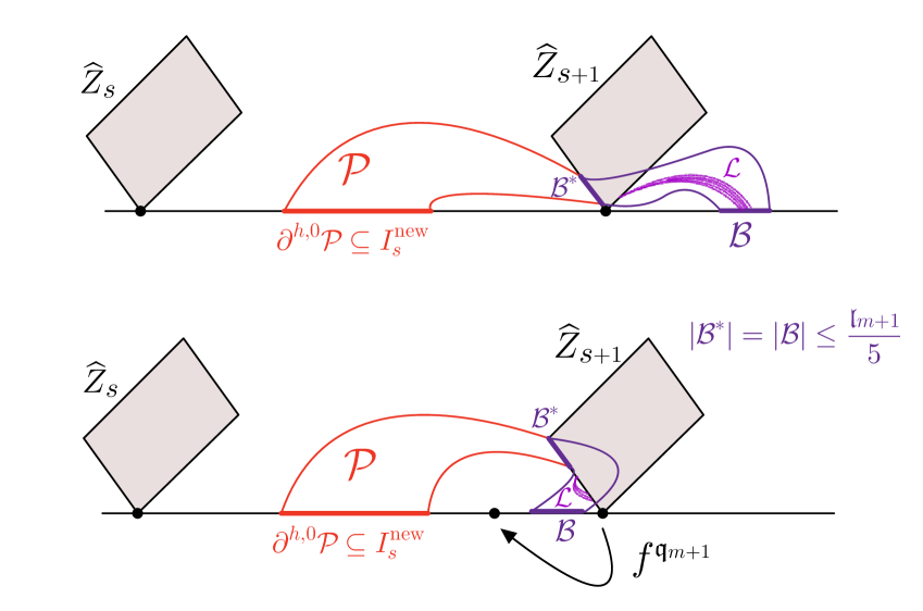
Figure 10. Illustration to the construction of a lamination $\displaystyle\mathcal{L}$. The rectangle $\displaystyle\mathcal{P}$ (red and purple) overflows its lift (the red part) before submerging into the pseudo-bubble $\displaystyle{\widehat{Z}}_{s+1}$. Localizing the submergence, we construct a lamination $\displaystyle\mathcal{L}\subset\mathcal{P}$ (light purple) outside of $\displaystyle{\widehat{Z}}_{s+1}$. There might be several configurations. Observe that if $\displaystyle\mathcal{B}$ intersects $\displaystyle T_{s}$ (bottom figure), then the intersection is combinatorially close to $\displaystyle{\widehat{Z}}_{s+1}$.

1. Let $\displaystyle{\mathcal{K}}_{m}\equiv K_{\mathfrak{q}_{m+1}}=f^{-\mathfrak{q}_{m+1}}(\overline{Z})$, which we identify as a subset of $\displaystyle V$ via (IV^k) in the definition of $\displaystyle\psi^{\bullet}$-ql Siegel map (see §2.1). Let $\displaystyle Z_{s+1}$ be the bubble at $\displaystyle a\in T_{s}\cap T_{s+1}$, i.e., the component of $\displaystyle{\mathcal{K}}_{m}-\overline{Z}$ that attached to $\displaystyle a$. Then there exists an interval $\displaystyle B^{*}$ on $\displaystyle\partial Z_{s+1}$ so that $\displaystyle f^{\mathfrak{q}_{m+1}}(B^{*})=B$, and up to $\displaystyle O(K)$, any vertical leaves in $\displaystyle\mathcal{P}$ passes through $\displaystyle B^{*}$.

2. We now replace $\displaystyle\overline{Z}_{s+1}$ with the associated pseudo-bubble $\displaystyle{\widehat{Z}}_{s+1}$ and replace $\displaystyle B^{*}$ with its grounded proejction $\displaystyle(B^{*})^{\operatorname{grnd}}$ onto $\displaystyle\partial{\widehat{Z}}_{s+1}$. We remove $\displaystyle O(1)$ curves in $\displaystyle\mathcal{P}$ that do not enter $\displaystyle{\widehat{Z}}_{s+1}$ through $\displaystyle(B^{*})^{\operatorname{grnd}}$.
   Let $\displaystyle Q\subseteq(B^{*})^{\operatorname{grnd}}$ be the interval bounded by the first intersection of the two left- and right-most vertical leaves in $\displaystyle\mathcal{P}$. Let $\displaystyle\gamma$ be a vertical leaf of $\displaystyle\mathcal{P}$. We define $\displaystyle\gamma^{\prime}$ as the shortest subarc connecting $\displaystyle Q$ to $\displaystyle\partial^{h,1}\mathcal{P}$, and set

   $$\mathcal{F}=\{\gamma^{\prime}:\gamma\in\mathcal{F}(\mathcal{P})\}.$$

3. Since $\displaystyle\mathcal{P}$ with $\displaystyle{\mathcal{W}}(\mathcal{P})\succeq{\boldsymbol{\chi}}^{0.9}K$ efficiently (up to $\displaystyle O(K)$) overflows its lift before $\displaystyle{\widehat{Z}}_{s+1}$, the family $\displaystyle\mathcal{F}$ (the part of $\displaystyle\mathcal{P}$ after $\displaystyle Q$) is extremely wide. We apply the argument in [DL3, Claim 6 in § 9] (i.e.,  the Grötzsch inequality) to conclude that

   $${\mathcal{W}}(\mathcal{F})\geq{\boldsymbol{\chi}}^{1.7}K.$$

4. As in [DL3, proof after Claim 6 in § 9], we replace $\displaystyle\mathcal{F}$ with a rectangle and apply [DL3, Lemma 6.9] to $\displaystyle\mathcal{F}$ to construct the lamination $\displaystyle\mathcal{L}\subset\mathcal{P}$ outside of $\displaystyle{\widehat{Z}}_{s+1}$ such that $\displaystyle\mathcal{L}$ emerges from a very small (of length $\displaystyle\ll\frac{{\mathfrak{l}}_{m+1}}{\lambda}$) interval very close to $\displaystyle Q$ and such that

   • either every leaf of $\displaystyle\mathcal{L}$ lands back at $\displaystyle\partial{\widehat{Z}}_{s+1}$ with the $\displaystyle\lambda$-separation from the interval where $\displaystyle\mathcal{L}$ starts; or

   • or every leaf of $\displaystyle\mathcal{L}$ lands at $\displaystyle\partial^{h,1}\mathcal{P}\subset\partial Z$. Since the combinatorial distance between $\displaystyle B$ and $\displaystyle B^{*}$ is $\displaystyle\geq\frac{2{\mathfrak{l}}_{m+1}}{5}$, we also have the $\displaystyle\lambda$-separation in this case. (Also, $\displaystyle\partial^{h,1}\mathcal{P}$ can be replaced with its grounded projection on $\displaystyle{\widehat{Z}}^{m}$.)

5. Finally, we apply the univalent pushforward $\displaystyle F^{\mathfrak{q}_{m+1}}_{*}$ to $\displaystyle\mathcal{L}$. The result is a required degeneration for Conclusion (III).

∎

6.2. Combinatorial Localization Property

The name ``Combinatorial Localization" is referred to Item (iii) of Lemma 6.4 below, where the original degeneration $\displaystyle K={\mathcal{W}}_{3}^{+}(I)\gg 1$ is localized on a grounded interval $\displaystyle J$ with $\displaystyle|J|<{\mathfrak{l}}_{j}<\frac{|I|}{T}$.

Lemma 6.2 is meant to be used near the transitional level where there is a level $\displaystyle m$ combinatorial interval $\displaystyle I$ witnessing a big degeneration $\displaystyle K={\mathcal{W}}_{3}^{+}(I)\gg 1$ with $\displaystyle K\succeq\ K_{F}/\mathfrak{q}_{m+1}$. Such degeneration is spread around and then, if applicable, localized and calibrated. The result is either Equidistribution (Item (i)), or Combinatorial Localization (Item (iii)), or a big external family (Item (ii)).

We remark that the equidistribution property in Item (i) can only be ruled out with a ``global external input'', see [DLu]. We also remark that if $\displaystyle{\widehat{Z}}^{m}$ were constructed in the ``optimal way'' (to consume most of the $\displaystyle{\mathcal{W}}^{+,{\operatorname{per}}}_{\lambda,{\operatorname{ext}},m}$-degeneration), then Item (ii) does not occur, which justifies the name of the lemma.

Lemma 6.4 (Equidistribution or Combinatorial Localization).

For every $\displaystyle\lambda,T\geq 1$, there exists $\displaystyle K_{T,\lambda}\gg 1$ so that the following holds.

Let $\displaystyle I\subseteq\partial Z$ be a level $\displaystyle m$ combinatorial interval with $\displaystyle{\mathcal{W}}^{+}_{5}(I)=K\geq K_{T,\lambda}$. Assume that $\displaystyle{\widehat{Z}}^{m}$ is a pseudo-Siegel disk. Then

1. either there is an  equidistribution of the degeneration: for every combinatorial interval $\displaystyle J\subset\partial Z$ of level $\displaystyle m$, we have

   $${\mathcal{W}}^{+,{\operatorname{ver}}}(J)\asymp K;$$

2. or there is a big  external degeneration: there exists an interval $\displaystyle J\subseteq\partial Z$ grounded rel $\displaystyle{\widehat{Z}}^{j+1}$ with $\displaystyle{\mathfrak{l}}_{j+1}\leq|J|<{\mathfrak{l}}_{j}\leq{\mathfrak{l}}_{m}$ and

   $${\mathcal{W}}^{+,{\operatorname{per}}}_{\lambda,{\operatorname{ext}},j}(J)\succeq K,$$

3. or there is a  combinatorial localization: there exists an interval $\displaystyle J\subseteq\partial Z$ grounded rel $\displaystyle{\widehat{Z}}^{j}$ with $\displaystyle|J|<{\mathfrak{l}}_{j}\leq\frac{{\mathfrak{l}}_{m}}{T}$ and

   $${\mathcal{W}}^{+}_{\lambda}(J)\succeq K.$$

Proof.

Let us first prove the following slightly weaker version of the lemma:

Claim. Assume that $\displaystyle{\mathcal{W}}_{3}^{+}(I)\geq K_{T,\lambda}/2$ holds for a level $\displaystyle m$ combinatorial interval $\displaystyle I\subseteq\partial Z$. Then either

1. for every interval $\displaystyle J=F^{i}(I)\subset\partial Z$, with $\displaystyle 0\leq i\leq 2\mathfrak{q}_{m+1}$, we have

   $${\mathcal{W}}^{+,{\operatorname{ver}}}(J)\asymp K;$$

or Conclusion (ii) or Conclusion (iii) of the Lemma 6.4 hold.

Proof of the claim.

We project the interval $\displaystyle I$ into the pseudo-Sigel disks $\displaystyle{\widehat{Z}}^{m}_{-k*}$ and use the simple transformation rule to spread around $\displaystyle{\widehat{Z}}^{m}$; see §3.7 and (3.25). We obtain that

$${\operatorname{proj}}^{\operatorname{grnd}}_{V,{\widehat{Z}}^{m}}\big({\mathcal{F}}_{3,Z}(I_{k})\big)\succeq K\qquad\qquad\text{ for all }J\equiv I_{i}=F^{i}(I).$$

Suppose Item (i’) does not hold. Then there exists $\displaystyle I_{s}=F^{s}(I)$ and a rectangle $\displaystyle\mathcal{R}$ of width $\displaystyle{\mathcal{W}}(\mathcal{R})\succeq K$ connecting the projections $\displaystyle I^{{\operatorname{grnd}},m}_{s}$ and $\displaystyle\big((3I_{s})^{c}\big)^{{\operatorname{grnd}},m}\cup V$ that submerges between $\displaystyle I^{{\operatorname{grnd}},m}_{s}$ and $\displaystyle\big((3I_{s})^{c}\big)^{{\operatorname{grnd}},m}$. By [DL3, Snake Lemma 6.1] and the fact $\displaystyle K\gg T,\lambda$, we obtain some grounded interval $\displaystyle I^{\prime}\subset\partial Z$ with $\displaystyle|I^{\prime}|\leq\frac{{\mathfrak{l}}_{m}}{T}$ so that $\displaystyle{\mathcal{W}}^{+}_{\lambda}(I^{\prime})\succeq K$. Let $\displaystyle k$ be the integer so that $\displaystyle{\mathfrak{l}}_{k+1}\leq|I^{\prime}|<{\mathfrak{l}}_{k}$. Suppose that Item (ii) does not hold, then we can apply the Calibration Lemma 6.1. In the case of Item (I) of the Calibration Lemma 6.1, we have Item (i). Otherwise, we have Item (iii). ∎

Let $\displaystyle J\subset\partial Z$ be an arbitrary combinatorial interval. Then there exists $\displaystyle J_{1}=F|_{\partial Z}^{-i_{1}}(J),J_{2}=|_{\partial Z}^{-i_{2}}(J)$ with $\displaystyle 0\leq i_{1}<i_{2}\leq 2\mathfrak{q}_{m+1}$ so that $\displaystyle I\subset J_{1}\cup J_{2}$. Note that $\displaystyle J_{1},J_{2}$ are in general not disjoint. Since $\displaystyle{\mathcal{W}}^{+}_{5}(I)=K\geq K_{T,\lambda}$, we conclude that $\displaystyle\max\{{\mathcal{W}}^{+}_{3}(J_{1}),{\mathcal{W}}^{+}_{3}(J_{2})\}\geq K_{T,\lambda}/2$. Without loss of generality, we assume that $\displaystyle{\mathcal{W}}^{+}_{3}(J_{1})\geq K_{T,\lambda}/2$. The lemma follows by applying the claim to $\displaystyle J_{1}$. ∎

7. A priori-bounds for $\displaystyle\psi^{\bullet}$-ql Siegel maps

In this section, we prove Theorem 1.3 restated as Theorems 7.1 and 7.5. The central induction is in the proof of Theorem 7.1 claiming the equidistribution property. Theorem 7.5 establishes explicit combinatorial thresholds for regularization $\displaystyle{\widehat{Z}}^{m+1}\leadsto{\widehat{Z}}^{m}$; the proof of Theorem 7.5 is in the a posteriori regime relative to Theorem 7.1.

The outline of the section is presented in §7.0.1. Let us briefly recall the main notations.

Let $\displaystyle F$ be an eventually-golden-mean $\displaystyle\psi^{\bullet}$-ql map as in §2.1. Recall that the definition of pseudo-Siegel disks for quadratic polynomials is introduced in [DL3, Definition 5.1]. The adjustments for $\displaystyle\psi^{\bullet}$-ql Siegel maps is introduced in §3.5.

Let $\displaystyle K_{F}\coloneqq{\mathcal{W}}^{\bullet}(F)$ be the width of $\displaystyle F$. Let $\displaystyle{\mathbf{K}}\gg 1$ be a sufficiently big threshold. Recall that the special transition level $\displaystyle{\mathbf{m}}_{F}$ for $\displaystyle F$ with respect to the threshold $\displaystyle{\mathbf{K}}$ is defined as follows.

• If $\displaystyle K_{F}\leq{\mathbf{K}}$, we set $\displaystyle{\mathbf{m}}_{F}\coloneqq-2$;

• Otherwise, we set $\displaystyle{\mathbf{m}}_{F}$ to be the level satisfying

  $$\frac{1}{{\mathfrak{l}}_{{\mathbf{m}}_{F}}}<\frac{K_{F}}{{\mathbf{K}}}\leq\frac{1}{{\mathfrak{l}}_{{\mathbf{m}}_{F}\ +1}}{\ \ }{\ \ }{\ \ }\begin{array}[]{c}\text{ or, }\\ \text{equivalently,}\end{array}{\ \ }{\ \ }{\ \ }{\ \ }\begin{array}[]{c}{\mathfrak{l}}_{{\mathbf{m}}_{F}}K_{F}>{\mathbf{K}},\text{ and}\vskip 5.69046pt\\ {\mathfrak{l}}_{{\mathbf{m}}_{F}\ +1}K_{F}\leq{\mathbf{K}}.\end{array}$$

In this section, we first prove the following a priori-bound for $\displaystyle\psi^{\bullet}$-ql map $\displaystyle F$, which is the first part of Theorem 1.3 and implies also the first part of Theorem 1.2 for quadratic-like maps as a special case.

Theorem 7.1 (Theorem 1.3: Equidistribution).

There exists an absolute constant $\displaystyle{\mathbf{K}}\gg 1$ so that the following holds.

Consider an eventually-golden-mean $\displaystyle\psi^{\bullet}$-ql map $\displaystyle F$ (see §2.1) of width $\displaystyle K_{F}={\mathcal{W}}^{\bullet}(F)$ and the special transition level $\displaystyle{\mathbf{m}}_{F}$ with respect to $\displaystyle{\mathbf{K}}$. Then there is a nested sequence of pseudo-Siegel disks $\displaystyle{\widehat{Z}}^{m},\ m\geq-1$ such that for every grounded interval $\displaystyle J\subset\partial Z$ with $\displaystyle{\mathfrak{l}}_{m+1}<|J|\leq{\mathfrak{l}}_{m}$ the following holds for the projection $\displaystyle J^{m}$ of $\displaystyle J$ to $\displaystyle{\widehat{Z}}^{m}$:

1. if $\displaystyle m>{\mathbf{m}}_{F}$, then

   $${\mathcal{W}}_{{\widehat{Z}}^{m}}^{+,{\operatorname{ver}}}(J^{m})=O(1){\ \ }{\ \ }\text{ and }{\ \ }{\ \ }{\mathcal{W}}_{3,{\widehat{Z}}^{m}}^{+,{\operatorname{per}}}(J^{m})\asymp 1,$$

2. if $\displaystyle m={\mathbf{m}}_{F}$, then

   $${\mathcal{W}}_{{\widehat{Z}}^{m}}^{+,{\operatorname{ver}}}(J^{m})=O({\mathfrak{l}}_{m}K_{F}){\ \ }{\ \ }\text{ and }{\ \ }{\ \ }{\mathcal{W}}_{3,{\widehat{Z}}^{m}}^{+,{\operatorname{per}}}(J^{m})=O\big(\sqrt{{\mathfrak{l}}_{m}K_{F}}\big),$$

3. if $\displaystyle m<{\mathbf{m}}_{F}$, then

   $${\mathcal{W}}_{{\widehat{Z}}^{m}}^{+,{\operatorname{ver}}}(J^{m})\asymp|J|K_{F}{\ \ }{\ \ }\text{ and }{\ \ }{\ \ }{\mathcal{W}}_{3,{\widehat{Z}}^{m}}^{+,{\operatorname{per}}}(J^{m})=O(1).$$

7.0.1. Outline of the section

The the central induction of the proof of Theorem 7.1 is encoded in Propositions 7.2 and is illustrated on the diagram in Figure 11. This induction is from deeper to shallower levels and is quite similar to the quadratic case; compare with the diagram on [DL3, Figure 27]. The key difference is the ``contradiction box $\displaystyle{\mathbf{A}}_{m}\geq\dots\gg{\mathbf{A}}_{m}$'' describing a possibility that an unexpected big vertical degeneration is developed. We also remark that Statements (a), (b), (c) of Proposition 7.2 are similar to the respective statements in [DL3, §10.0.1].

Proposition 7.2 is stated with an explicit universal constant $\displaystyle{\mathbf{K}}\asymp{\mathbf{K}}_{m}$, see (7.1), (7.2). (We find it convenient to slightly modify $\displaystyle{\mathbf{K}}$ into $\displaystyle{\mathbf{K}}_{m}$). Theorem 7.1 suppresses $\displaystyle{\mathbf{K}}$ within $\displaystyle O(1)\equiv O({\mathbf{K}})$. The choice of constants in the proof of Proposition 7.2 is summarized in §7.1.1. Constants $\displaystyle{\mathbf{t}},{\boldsymbol{\chi}},{\boldsymbol{\lambda}}_{\mathbf{t}}$ are selected as in the quadratic case. An additional constant $\displaystyle{\mathbf{L}}$ (tied to the ``contradiction box $\displaystyle{\mathbf{A}}_{m}\geq\dots\gg{\mathbf{A}}_{m}$'') is selected to accommodate Alternative (ii) of Amplification Theorem 5.1 so that (7.3) and thus (7.6) hold.

The proof of Theorem 7.1 is completed in Propositions 7.3 and 7.4, where the equidistribution of the vertical families is justified. These propositions rely on Lemma 6.4, ``Equidistribution or Combinatorial Localization''. Item (iii) of Lemma 6.4 leads to a contradiction by constructing a bigger degeneration. To accommodate such an argument, an additional constant $\displaystyle{\mathbf{T}}\gg{\mathbf{L}}$ is selected so that (7.5) holds. (The constant $\displaystyle{\mathbf{T}}$ does not directly influence the main induction of Proposition 7.2.)

The constant $\displaystyle{\mathbf{K}}$, the key geometric threshold, is selected last.

7.1. Deep and transitional levels

We will prove Theorem 7.1 by induction from deep to shallow levels as follows. We will show that there are

$${\boldsymbol{\lambda}}\gg 1,\quad{\mathbf{L}}\gg_{{\boldsymbol{\lambda}}}1,\quad{\mathbf{T}}\gg{\mathbf{L}},\quad\text{ and }\quad{\mathbf{K}}\ \gg_{{\boldsymbol{\lambda}},{\mathbf{T}}}\ \ 1$$

such that the following properties hold.

Consider an eventually-golden-mean $\displaystyle\psi^{\bullet}$-ql map $\displaystyle F$ of width $\displaystyle K_{F}={\mathcal{W}}^{\bullet}(F)$ and the transition level $\displaystyle{\mathbf{m}}_{F}$ with respect to $\displaystyle{\mathbf{K}}$. We define the average vertical degeneration at level $\displaystyle m$ by

$${\mathbf{A}}_{m}:={\mathfrak{l}}_{m}K_{F}.$$

We define the degeneration threshold for $\displaystyle m\geq{\mathbf{m}}_{F}$ by

(7.1) $${\mathbf{K}}_{m}:=\frac{{\mathbf{K}}}{{\mathbf{T}}}+{\mathbf{L}}\cdot{\mathbf{A}}_{m}$$

It easily follows from definition that for $\displaystyle m>{\mathbf{m}}_{F}$, the constants $\displaystyle{\mathbf{K}}_{m}$ and $\displaystyle{\mathbf{K}}$ are comparable:

(7.2) $$\begin{matrix}{\mathbf{K}}_{m}\ \asymp_{{\mathbf{T}}}\ {\mathbf{K}}/{\mathbf{T}},\qquad\quad&\text{ i.e., }\quad{\mathbf{K}}/{\mathbf{T}}\leq{\mathbf{K}}_{m}\leq 3{\mathbf{L}}{\mathbf{K}}\ll{\mathbf{T}}{\mathbf{K}},\\ {\mathbf{K}}_{m}\ \to\ {\mathbf{K}}/{\mathbf{T}}\qquad\quad&\text{ monotonically as }\quad m\to\infty.\end{matrix}$$

By design, $\displaystyle{\mathbf{K}}\ \asymp_{\mathbf{T}}\ {\mathbf{K}}_{m}\ \gg_{{\boldsymbol{\lambda}},{\mathbf{T}}}\ \ 1$ allows arbitrary large (but still fixed) dependence on all combinatorial constants; see §7.1.1.

We now state a quantified version of Theorem 7.1 at the deep and transitional levels.

Proposition 7.2.

For all $\displaystyle m\geq{\mathbf{m}}_{F}$,

1. there exists a geodesic pseudo-Siegel disk $\displaystyle{\widehat{Z}}^{m}$ so that

   $${\mathcal{W}}^{+,{\operatorname{per}}}_{{\boldsymbol{\lambda}},{\operatorname{ext}},m}(I)=O(\sqrt{{\mathbf{K}}_{m}})$$

   for every interval $\displaystyle I$ grounded rel $\displaystyle{\widehat{Z}}^{m}$ with $\displaystyle{\mathfrak{l}}_{m+1}\leq|I|\leq{\mathfrak{l}}_{m}$. (In other words, $\displaystyle{\widehat{Z}}^{m}$ consumes all but $\displaystyle O(\sqrt{{\mathbf{K}}_{m}})$-external $\displaystyle\lambda$-separated rel $\displaystyle m$ families.)

2. $\displaystyle{\mathcal{W}}_{\boldsymbol{\lambda}}^{+}(I)\leq(2{\boldsymbol{\chi}}){\mathbf{K}}_{m}$ for every grounded rel $\displaystyle{\widehat{Z}}^{m}$ interval $\displaystyle m$ with $\displaystyle|I|\leq{\mathfrak{l}}_{m}$, where $\displaystyle{\boldsymbol{\chi}}$ is the constant from Calibration Lemma 6.1.

3. $\displaystyle{\mathcal{W}}_{\boldsymbol{\lambda}}^{+}(I)\leq{\mathbf{K}}_{m}$ for every combinatorial interval $\displaystyle I$ of level $\displaystyle\geq m$.

7.1.1. The choice of constants in the proof of Proposition 7.2

We first choose $\displaystyle{\mathbf{t}}\gg{\boldsymbol{\chi}}$, where $\displaystyle{\boldsymbol{\chi}}$ is the constant in the Calibration Lemma 6.1. We choose $\displaystyle{\boldsymbol{\lambda}}:={\boldsymbol{\lambda}}_{{\mathbf{t}}}$ as in the Amplification Theorem 5.1.

Recall that $\displaystyle{\mathfrak{l}}_{m}\asymp\frac{1}{\mathfrak{q}_{m+1}}$. Let $\displaystyle{\mathbf{L}}\gg_{\boldsymbol{\lambda}}1$ be chosen so that second alternative in Amplification Theorem 5.1 $\displaystyle K_{F}\succeq_{{\boldsymbol{\lambda}}_{\mathbf{t}}}K\mathfrak{q}_{m+1}$ gives

(7.3) $${\mathbf{A}}_{m}={\mathfrak{l}}_{m}K_{F}\gg\frac{K}{{\mathbf{L}}},$$

see (7.6) for the application of (7.3).

The constant $\displaystyle{\mathbf{T}}$ (the input for Item (iii) of Lemma 6.4) is chosen so that

(7.4) $${\mathbf{T}}\gg{\mathbf{L}}.$$

Finally, the constant $\displaystyle{\mathbf{K}}$ is chosen so that

(7.5) $${\mathbf{K}}\ \gg_{{\mathbf{T}}}\ \ {\mathbf{K}}_{\mathbf{t}},$$

where $\displaystyle{\mathbf{K}}_{\mathbf{t}}$ is the constant in the Amplification Theorem 5.1.

Figure 11. Statements (a), (b), and (c) are proved by contradiction: if one of the statements is violated on levels $\displaystyle m$ or $\displaystyle m+1/2$, then there will be even bigger violation on deeper scales. Here ``$\displaystyle m$'' indicates level $\displaystyle m$ combinatorial intervals, ``$\displaystyle m+1/2$'' indicates intervals with $\displaystyle{\mathfrak{l}}_{m}\geq|I|\geq{\mathfrak{l}}_{m+1}$, and ``$\displaystyle m+1$'' indicates intervals with $\displaystyle|I|\leq{\mathfrak{l}}_{m+1}$. The dashed arrows illustrate the decomposition $\displaystyle{\mathcal{F}}_{\boldsymbol{\lambda}}^{+}={\mathcal{F}}^{+,{\operatorname{per}}}_{{\boldsymbol{\lambda}},{\operatorname{ext}},m}\sqcup{\mathcal{F}}^{+,{\operatorname{per}}}_{{\boldsymbol{\lambda}},{\operatorname{div}},m}\sqcup{\mathcal{F}}^{+,{\operatorname{ver}}}$.

Proof of Proposition 7.2.

The proof is similar in the quadratic polynomial setting, with only minor modifications. We summarize the induction steps as follows, see Figure 11 for an illustration.

First, consider $\displaystyle m\geq{\mathbf{m}}_{F}$ with $\displaystyle{\mathfrak{l}}_{m}\leq|\theta_{0}|/(2{\boldsymbol{\lambda}}+4)$, where $\displaystyle\theta_{0}$ is the rotation number for $\displaystyle F$.

1. Suppose Statement (c) is violated at level $\displaystyle m$, i.e., there exists a level $\displaystyle m$ combinatorial interval $\displaystyle I$ with $\displaystyle K:={\mathcal{W}}^{+}_{{\boldsymbol{\lambda}}}(I)>{\mathbf{K}}_{m}$. Then by Amplification Theorem 5.1 and (7.3),

   • either

     (7.6) $${\mathbf{A}}_{m}\gg\frac{K}{{\mathbf{L}}}>\frac{{\mathbf{K}}_{m}}{{\mathbf{L}}}=\frac{{\mathbf{K}}/{\mathbf{T}}+{\mathbf{L}}\cdot{\mathbf{A}}_{m}}{{\mathbf{L}}}\geq{\mathbf{A}}_{m}$$

     which is a contradiction; or

   • there exists an interval $\displaystyle J$ with $\displaystyle|J|<{\mathfrak{l}}_{m}$ and

     $${\mathcal{W}}^{+}_{{\boldsymbol{\lambda}}}(J)\gg(2{\boldsymbol{\chi}}){\mathbf{K}}_{m}\geq(2{\boldsymbol{\chi}}){\mathbf{K}}_{j}\text{ for any }j\geq m+1.$$

     Thus, Statement (b) is violated for some interval $\displaystyle J$ at level $\displaystyle\geq m+1$.

2. Suppose Statement (a) is violated at level $\displaystyle m$, i.e., a pseudo-Siegel disk $\displaystyle{\widehat{Z}}$ can not be constructed to absorb all but $\displaystyle O(\sqrt{{\mathbf{K}}_{m}})$-external rel $\displaystyle m$ families. Then by the exponential boost in Theorem 4.7,

   • either there exists some interval $\displaystyle J$ with $\displaystyle|J|\leq{\mathfrak{l}}_{m+1}$ and

     $${\mathcal{W}}^{+}_{{\boldsymbol{\lambda}}}(J)\geq a^{\sqrt{{\mathbf{K}}_{m}}}\gg(2{\boldsymbol{\chi}}){\mathbf{K}}_{m}\geq(2{\boldsymbol{\chi}}){\mathbf{K}}_{j}$$

     for any $\displaystyle j\geq m+1$, and for some fixed $\displaystyle a>1$. Thus Statement (b) is violated for some interval $\displaystyle J$ at level $\displaystyle\geq m+1$; or

   • there exists some interval $\displaystyle J$ with $\displaystyle{\mathfrak{l}}_{m+1}<|J|\leq{\mathfrak{l}}_{m}$ and

     $${\mathcal{W}}^{+,{\operatorname{per}}}_{{\boldsymbol{\lambda}},{\operatorname{div}},m}(J)+{\mathcal{W}}^{+,{\operatorname{ver}}}(J)\geq a^{\sqrt{{\mathbf{K}}_{m}}}\gg(2{\boldsymbol{\chi}}){\mathbf{K}}_{m}$$

     for some $\displaystyle a>1$ is fixed. Then by Calibration Lemma 6.1, either Statement (c) or Statement (b) is violated on levels $\displaystyle\geq m+1$; or $\displaystyle{\mathbf{A}}_{m}=K_{F}{\mathfrak{l}}_{m}\geq{\mathcal{W}}^{+}_{\boldsymbol{\lambda}}(J)\geq{\mathbf{K}}_{m}\gg{\mathbf{A}}_{m}$, which is not possible.

3. Suppose Statement (b) is violated at level $\displaystyle m$. By the decomposition

   $${\mathcal{F}}_{\boldsymbol{\lambda}}^{+}(I)={{\mathcal{F}}^{+,{\operatorname{per}}}_{{\boldsymbol{\lambda}},{\operatorname{ext}},m}(I)\sqcup{\mathcal{F}}^{+,{\operatorname{per}}}_{{\boldsymbol{\lambda}},{\operatorname{div}},m}(I)\sqcup{\mathcal{F}}^{+,ver}(I)},$$

   we have the following two cases.

   • $\displaystyle{\mathcal{W}}^{+,{\operatorname{per}}}_{{\boldsymbol{\lambda}},{\operatorname{ext}},m}(I)\geq{\mathbf{K}}_{m}\gg\sqrt{{\mathbf{K}}_{m}}$. Thus Statement (a) is violated at level $\displaystyle m$; or

   • $\displaystyle{\mathcal{W}}^{+,{\operatorname{per}}}_{{\boldsymbol{\lambda}},{\operatorname{div}},m}(I)+{\mathcal{W}}^{+,ver}(I)>(1.5{\boldsymbol{\chi}}){\mathbf{K}}_{m}$. Then by Calibration Lemma 6.1, either Statement (c) or Statement (b) is violated on levels $\displaystyle\geq m+1$; or $\displaystyle{\mathbf{A}}_{m}=K_{F}{\mathfrak{l}}_{m}\geq{\mathcal{W}}^{+}_{\boldsymbol{\lambda}}(I)\geq{\mathbf{K}}_{m}\gg{\mathbf{A}}_{m}$, which is not possible.

Let $\displaystyle{\mathbf{s}}_{\theta_{0}}$ be the smallest integer so that $\displaystyle{\mathfrak{l}}_{\mathbf{s}}\leq|\theta_{0}|/(2{\boldsymbol{\lambda}}+4)$. Then $\displaystyle{\mathbf{s}}_{\theta_{0}}\leq 2\log_{2}(2{\boldsymbol{\lambda}}+4)$, i.e., there is a uniform bound on the number of levels $\displaystyle m$ with $\displaystyle{\mathfrak{l}}_{m}\leq|\theta_{0}|/(2{\boldsymbol{\lambda}}+4)$. Thus, by increasing the constants, Proposition 7.2 follows (see [DL3, Lemma 10.4] for more details). ∎

Finally, note that Proposition 7.2 gives the bound for $\displaystyle{\mathcal{W}}^{+,{\operatorname{ver}}}_{{\widehat{Z}}^{m}}$ and $\displaystyle{\mathcal{W}}_{{\boldsymbol{\lambda}},{\widehat{Z}}^{m}}^{+,{\operatorname{per}}}$. To obtain the bound for $\displaystyle{\mathcal{W}}_{3,{\widehat{Z}}^{m}}^{+,{\operatorname{per}}}$, we apply exactly the same argument as in [DL3, §10.1.1], and obtain Theorem 7.1 for $\displaystyle m\geq{\mathbf{m}}_{F}$.

7.2. Equidistribution on trnasitional and shallow levels

The next proposition is an application of Proposition 7.2 and Lemma 6.4, ``Equidistribution or Combinatorial Localization''.

Proposition 7.3 (Equidistribution: the transitional level).

Vertical degenerations on level $\displaystyle{\mathbf{m}}_{F}$ combinatorial intervals are equidistributed, i.e., for any interval $\displaystyle I\in\mathfrak{D}_{{\mathbf{m}}_{F}}$ in the $\displaystyle{\mathbf{m}}_{F}$-th diffeo-tiling, we have

$${\mathcal{W}}^{+,{\operatorname{ver}}}(I)\asymp{\mathbf{A}}_{{\mathbf{m}}_{F}},$$

where $\displaystyle{\mathbf{A}}_{{\mathbf{m}}_{F}}=K_{F}{\mathfrak{l}}_{{\mathbf{m}}_{F}}$ is the average vertical degeneration at level $\displaystyle{\mathbf{m}}_{F}$.

Proof.

The proof is by contradiction. Suppose that vertical degenerations on level $\displaystyle{\mathbf{m}}_{F}$ combinatorial intervals are not equidistributed.

Since the average vertical degeneration is $\displaystyle{\mathbf{A}}_{{\mathbf{m}}_{F}}$, there exists $\displaystyle I\in\mathfrak{D}_{{\mathbf{m}}_{F}}$ in the $\displaystyle{\mathbf{m}}_{F}$-th diffeo-tiling with

$${\mathcal{W}}^{+,{\operatorname{ver}}}(I)=K\succeq{\mathbf{A}}_{{\mathbf{m}}_{F}}.$$

By Proposition 7.2, for any $\displaystyle m\geq{\mathbf{m}}_{F}$, $\displaystyle{\mathcal{W}}^{+,{\operatorname{per}}}_{{\boldsymbol{\lambda}},{\operatorname{ext}},m}(I)=O(\sqrt{{\mathbf{K}}_{m}})\ll K$. Thus by Combinatorial Localization Lemma 6.4, there exists a grounded interval $\displaystyle J\subseteq\partial{\widehat{Z}}^{j}$ with $\displaystyle|J|<{\mathfrak{l}}_{j}\leq\frac{{\mathfrak{l}}_{{\mathbf{m}}_{F}}}{{\mathbf{T}}}$ and $\displaystyle{\mathcal{W}}^{+}_{\lambda}(J)\succeq K$. Since $\displaystyle{\mathbf{T}}\gg{\boldsymbol{\chi}},{\mathbf{L}}$ and $\displaystyle K_{F}{\mathfrak{l}}_{{\mathbf{m}}_{F}}\geq{\mathbf{K}}\gg{\boldsymbol{\chi}}{\mathbf{K}}/{\mathbf{T}}$, we conclude that

$$\displaystyle{\mathbf{A}}_{{\mathbf{m}}_{F}} \displaystyle=K_{F}{\mathfrak{l}}_{{\mathbf{m}}_{F}}\gg(2{\boldsymbol{\chi}})({\mathbf{K}}/{\mathbf{T}}+\frac{{\mathbf{L}}K_{F}{\mathfrak{l}}_{{\mathbf{m}}_{F}}}{{\mathbf{T}}})$$

$$\displaystyle\geq(2{\boldsymbol{\chi}})({\mathbf{K}}/{\mathbf{T}}+{\mathbf{L}}K_{F}{\mathfrak{l}}_{j})=(2{\boldsymbol{\chi}}){\mathbf{K}}_{j}.$$

Therefore, $\displaystyle{\mathcal{W}}^{+}_{\boldsymbol{\lambda}}(J)\gg(2{\boldsymbol{\chi}}){\mathbf{K}}_{j}$, which is a contradiction to Statement (b) in Proposition 7.2 at level $\displaystyle j\geq{\mathbf{m}}_{F}+1$. ∎

Finally, applying Proposition 7.3 and parallel law, we obtain:

Proposition 7.4 (Equidistribution: shallows levels).

Let $\displaystyle m<{\mathbf{m}}_{F}$, and $\displaystyle{\widehat{Z}}^{m}={\widehat{Z}}^{{\mathbf{m}}_{F}}$. Let $\displaystyle{\mathfrak{l}}_{m+1}<J\leq{\mathfrak{l}}_{m}$ be a grounded interval. Then

$${\mathcal{W}}_{{\widehat{Z}}^{m}}^{+,{\operatorname{ver}}}(J^{m})\asymp|J|K_{F}{\ \ }{\ \ }\text{ and }{\ \ }{\ \ }{\mathcal{W}}_{3,{\widehat{Z}}^{m}}^{+,{\operatorname{per}}}(J^{m})=O(1).$$

Proof.

Since $\displaystyle m<{\mathbf{m}}_{F}$, there exists $\displaystyle N=N(J)$ so that $\displaystyle I\subset J\subset I^{\prime}$, where $\displaystyle I$ is a union of $\displaystyle N$ level-$\displaystyle{\mathbf{m}}_{F}$ combinatorial intervals, and $\displaystyle I^{\prime}$ is a union of $\displaystyle N+2$ level-$\displaystyle{\mathbf{m}}_{F}$ combinatorial intervals. By Proposition 7.3, the vertical degeneration on a level-$\displaystyle{\mathbf{m}}_{f}$ combinatorial interval is comparable to $\displaystyle{\mathbf{A}}_{{\mathbf{m}}_{F}}$. Thus, by parallel law (see, for e.g. [DL3, A.1.4]), $\displaystyle{\mathcal{W}}_{{\widehat{Z}}^{m}}^{+,{\operatorname{ver}}}(J^{m})\succeq N{\mathbf{A}}_{{\mathbf{m}}_{F}}\asymp|J|K_{F}$. Since the same argument also holds for $\displaystyle\partial Z\setminus J$, we conclude that $\displaystyle{\mathcal{W}}_{{\widehat{Z}}^{m}}^{+,{\operatorname{ver}}}(J^{m})\asymp|J|K_{F}$.

On the other hand, since each component of $\displaystyle 3J\setminus J$ contains a level-$\displaystyle{\mathbf{m}}_{F}$ combinatorial interval $\displaystyle I_{\pm}$, any arc in $\displaystyle{\mathcal{F}}^{+,{\operatorname{per}}}_{3,{\widehat{Z}}^{m}}(J^{m})$ intersects an arc in $\displaystyle{\mathcal{F}}^{+,{\operatorname{ver}}}_{{\widehat{Z}}^{m}}(I_{\pm}^{m})$. Since $\displaystyle{\mathcal{W}}^{+,{\operatorname{ver}}}_{{\widehat{Z}}^{m}}(I_{\pm}^{m})={\mathcal{W}}^{+,{\operatorname{ver}}}(I_{\pm})+O(1)\asymp{\mathbf{A}}_{{\mathbf{m}}_{F}}\gg 1$, we conclude that $\displaystyle{\mathcal{W}}^{+,{\operatorname{per}}}_{3,{\widehat{Z}}^{m}}(J^{m})=O(1)$. ∎

7.2.1. Proof of Theorem 7.1

The theorem follows from Propositions 7.2, 7.3, and 7.3. ∎

7.3. Pseudo-Siegel disks with explicit combinatorial thresholds

The next theorem provides a construction of pseudo-Siegel disks with explicit combinatorial thresholds on all levels except transitional:

Theorem 7.5 (Theorem 1.3: combinatorial thresholds).

Let $\displaystyle{\mathbf{m}}_{F}$ be the transitional level of $\displaystyle F$ as in Theorem 7.1. There exist a sufficiently big $\displaystyle{\mathbf{M}}\gg 1$ and an increasing function $\displaystyle H\colon\mathbb{R}_{>0}\to\mathbb{R}_{\geq{\mathbf{M}}}$ such that the following holds. We set

(7.7) $$\displaystyle\begin{split}{\mathbf{M}}_{m}&\coloneqq\begin{cases}{\mathbf{M}},\,\,\text{ if $\displaystyle m>{\mathbf{m}}_{F}$,}\\ H({\mathfrak{l}}_{m}K_{F})\,\,\text{ if $\displaystyle m={\mathbf{m}}_{F}$,}\\ \infty,\,\,\text{ if $\displaystyle m<{\mathbf{m}}_{F}$.}\end{cases}\end{split}$$

Then geodesic pseudo-Siegel disks $\displaystyle{\widehat{Z}}^{m}$ for Theorem 7.1 can be constructed explicitly as follows. For every (near-parabolic) $\displaystyle m$ with $\displaystyle{\mathfrak{l}}_{m}>{\mathbf{M}}_{m}{\mathfrak{l}}_{m+1}$, add geodesic parabolic fjords $\displaystyle\widehat{\mathfrak{F}}_{I}$ at depth $\displaystyle\left\lfloor e^{\sqrt{\ln{\mathbf{M}}_{m}}}\right\rfloor$, see for details §7.3.2.

Consequently, $\displaystyle{\widehat{Z}}^{-1}$ is $\displaystyle\mu(K_{F})$-qc disk; i.e. the dilatation of the qc disk $\displaystyle{\widehat{Z}}^{-1}$ is bounded in terms of $\displaystyle K_{F}$.

As it is indicated in Theorem 7.5, we say a level $\displaystyle m$ is near-parabolic if and only if $\displaystyle{\mathfrak{l}}_{m}>{\mathbf{M}}_{m}{\mathfrak{l}}_{m+1}$; otherwise $\displaystyle m$ is non-parabolic. Since $\displaystyle F$ is eventually-golden-mean, all sufficiently deep levels $\displaystyle m\gg_{F}\ 1$ are non-parabolic. In short, $\displaystyle{\mathbf{M}}_{m}$ will be a combinatorial threshold for regularization: if $\displaystyle\frac{{\mathfrak{l}}_{m}}{{\mathfrak{l}}_{m+1}}\geq{\mathbf{M}}_{m}$, then $\displaystyle{\widehat{Z}}^{m+1}$ is regularized into $\displaystyle{\widehat{Z}}^{m}$ at depth $\displaystyle e^{\sqrt{\ln{\mathbf{M}}_{m}}}$, see §7.3.2; otherwise $\displaystyle{\widehat{Z}}^{m}:={\widehat{Z}}^{m+1}$. We remark that by our definition of $\displaystyle{\mathbf{M}}_{m}$, if $\displaystyle m<{\mathbf{m}}_{F}$, then we always set $\displaystyle{\widehat{Z}}^{m}:={\widehat{Z}}^{m+1}$.

Proof of Theorem 7.5.

The explicit threshold on the regularization follows from Lemma 7.6 below. It implies that the Log-Rule of Theorem 4.4 kicks off at an explicit threshold. Therefore, the regularization $\displaystyle{\widehat{Z}}^{m+1}\leadsto{\widehat{Z}}^{m}$ can also be achieved at the explicit threshold as required by Theorem 4.7: if the regularization fails, then, for a universal $\displaystyle a>1$, either

• there is a degeneration $\displaystyle\succeq a^{\sqrt{{\mathbf{M}}_{m}}}$ on a deeper level,

• or the vertical degeneration is $\displaystyle\succeq a^{\sqrt{{\mathbf{M}}_{m}}}\mathfrak{q}_{m+1}$;

compare with Item ``not (a)'' on Figure 11.

The quasiconformality claim is a non-dynamical statement that follows in the same way as in [DL3, Section 11]. More precisely, we introduce a nest of tilings $\displaystyle\mathcal{T}(\partial{\widehat{Z}}^{m})$ on $\displaystyle\partial{\widehat{Z}}^{m}$ by projecting the diffeo-tiling of $\displaystyle\partial\mathbb{Z}$ onto $\displaystyle\partial{\widehat{Z}}^{-1}$. On dams, the tiling is introduced geometrically in the same way as in [DL3, §11.3.]. Applying [DL3, Lemma 11.3] and using the main estimates, we obtain the quasiconformality claim. ∎

7.3.1. Combinatorial threshold for Log-Rule

Since Theorem 7.1 is established, we are now in the a posteriori setting where the quantities $\displaystyle{\mathbf{K}}_{m},\ m>{\mathbf{m}}_{F}$, in Proposition 7.2 are absolute; we write $\displaystyle{\mathbf{K}}_{m}=O(1)$.

For the following lemma, recall that the notations of $\displaystyle x,y,v,w$ are introduced in § 4.3; see Figure 7.

Lemma 7.6.

For levels $\displaystyle m>{\mathbf{m}}_{F}$, the interval $\displaystyle[x,y]$ satisfies

(7.8) $$\operatorname{dist}(v,x)\ \asymp\ \operatorname{dist}(y,w)\ \asymp\ {\mathfrak{l}}_{m+1}.$$

If $\displaystyle\operatorname{dist}(v,w)\gg 1$, then $\displaystyle[x,y]$ is non-empty and satisfies (7.8).

For $\displaystyle m={\mathbf{m}}_{F}$, the interval $\displaystyle[x,y]$ satisfies

(7.9) $$\operatorname{dist}(v,x)\ \asymp_{({\mathfrak{l}}_{m+1}K_{F})}\ \operatorname{dist}(y,w)\ \asymp_{({\mathfrak{l}}_{m+1}K_{F})}\ {\mathfrak{l}}_{m+1}.$$

Proof.

The argument is the same as in [DL3, §10.2]. We assume that $\displaystyle[v,x]\asymp[y,w]$ are long, we split these intervals into the $\displaystyle\bigcup_{k}X^{k}$ and $\displaystyle\bigcup_{k}Y^{k}$ and estimate the dual family to deduce (7.10) and (7.11). For $\displaystyle m={\mathbf{m}}_{F}$, the vertical family affects ``$\displaystyle\succeq$''.

Assume that $\displaystyle x$ is sufficiently far from $\displaystyle v$. As in [DL3, §10.2], we present $\displaystyle[v,x]$ a concatenation of $\displaystyle X^{1}\cup X^{2}\cup\dots\cup X^{K}$, where $\displaystyle|X^{1}|=10{\mathfrak{l}}_{m+1}$ and $\displaystyle|X^{i+1}|=2|X^{i}|$. Similarly, present $\displaystyle[y,w]$ as a concatenation of $\displaystyle Y^{k}\cup Y^{k-1}\cup\dots\cup Y^{1}$ satisfying the same properties: $\displaystyle|Y^{1}|=10{\mathfrak{l}}_{m+1}$ and $\displaystyle|Y^{i+1}|=2|Y^{i}|$.

As in [DL3, Lemma 10.5], we claim that

(7.10) $${\mathcal{W}}^{+,{\operatorname{per}}}_{{\operatorname{ext}},m}(X^{k},Y^{k})\ \succeq 1\qquad\qquad\text{ if }m>{\mathbf{m}}_{F},$$

and

(7.11) $${\mathcal{W}}^{+,{\operatorname{per}}}_{{\operatorname{ext}},m}(X^{k},Y^{k})\ \succeq_{({\mathfrak{l}}_{m+1}K_{F})}\ \ 1\qquad\qquad\text{ if }m={\mathbf{m}}_{F},$$

Proof of the Claim.

Following notations of [DL3, Lemma 10.5], we denote by $\displaystyle T^{k}$ the interval between $\displaystyle X^{k}$ and $\displaystyle Y^{k}$ and we have $\displaystyle T^{k}=X^{k+1}\cup T^{k+1}\cup Y^{k+1}$. To deduce (7.10) and (7.11), we need to estimate from above the width of the dual family:

$${\mathcal{W}}^{+,{\operatorname{ver}}}(T^{k})+{\mathcal{W}}^{+,{\operatorname{per}}}_{{\mathcal{K}}_{m}}(T^{k},\partial{\mathcal{K}}_{m}\setminus T^{k-1}).$$

For $\displaystyle m>{\mathbf{m}}_{F}$, we have $\displaystyle{\mathcal{W}}^{+,{\operatorname{ver}}}(T^{k})=O(1)$. For $\displaystyle m={\mathbf{m}}_{F}$, we have $\displaystyle{\mathcal{W}}^{+,{\operatorname{ver}}}(T^{k})\asymp K_{F}{\mathfrak{l}}_{m}+O(1)$.

The argument to estimate $\displaystyle{\mathcal{W}}^{+,{\operatorname{per}}}_{{\mathcal{K}}_{m}}(T^{k},\partial{\mathcal{K}}_{m}\setminus T^{k-1})$ is the same as in [DL3, Lemma 10.5]: apply a univalent pushforward $\displaystyle f^{\mathfrak{q}_{m+1}}$ to replace $\displaystyle{\mathcal{K}}_{m}$ with $\displaystyle\overline{Z}$, and then use the Shift Argument to bound the $\displaystyle{\mathcal{W}}^{+,{\operatorname{per}}}_{{\operatorname{ext}},m}$-component and the Calibration Lemma to bound the $\displaystyle{\mathcal{W}}^{+,{\operatorname{per}}}_{{\operatorname{div}},m}$-component. ∎

Applying the parallel law, we deduce that $\displaystyle{\mathcal{W}}^{+,{\operatorname{per}}}_{{\operatorname{ext}},m}([v,x],[y,w])$ is sufficiently wide if $\displaystyle x,y$ are sufficiently far from $\displaystyle v,w$ as required. ∎

7.3.2. Construction of parabolic fjord $\displaystyle\widehat{\mathfrak{F}}_{I}$ and $\displaystyle S^{\operatorname{inn}}_{I}$

Consider a near-parabolic level $\displaystyle m$. Let $\displaystyle I=[a,b]\in\mathfrak{D}_{m}$ be an interval in the $\displaystyle m$th diffeo-tiling of $\displaystyle\partial Z$. Choose $\displaystyle a^{\prime},b^{\prime}\in I$ with $\displaystyle a<a^{\prime}<b^{\prime}<b$ such that

$$\operatorname{dist}(a,a^{\prime})=\operatorname{dist}(b^{\prime},b)=\left\lfloor e^{\sqrt{\ln{\mathbf{M}}_{m}}}\right\rfloor\ {\mathfrak{l}}_{m+1}$$

and set $\displaystyle\beta_{I}$ to be the hyperbolic geodesic of $\displaystyle V\setminus\overline{Z}$ connecting $\displaystyle a^{\prime},b^{\prime}$. This defines the parabolic fjord $\displaystyle\widehat{\mathfrak{F}}_{I}$. We remark that since the level $\displaystyle m$ is near-parabolic, we have

$$|I|=\operatorname{dist}(a,b)\asymp{\mathfrak{l}}_{m}\geq{\mathbf{M}}_{m}{\mathfrak{l}}_{m+1}\gg\left\lfloor e^{\sqrt{\ln{\mathbf{M}}_{m}}}\right\rfloor\ {\mathfrak{l}}_{m+1}.$$

To construct $\displaystyle S^{\operatorname{inn}}_{I}$, we choose a sufficiently big $\displaystyle{\mathbf{v}}\gg 1$ with the understanding that $\displaystyle e^{\sqrt{\ln{\mathbf{M}}_{m}}}\gg{\mathbf{v}}$. Choose $\displaystyle a^{\prime\prime}\in[a,a^{\prime}]$ and $\displaystyle b^{\prime\prime}\in[b^{\prime},b]$ such that

(7.12) $$\operatorname{dist}(a,a^{\prime\prime})=\operatorname{dist}(b^{\prime\prime},b)=\left\lfloor\frac{e^{\sqrt{\ln{\mathbf{M}}_{m}}}}{{\mathbf{v}}}\right\rfloor{\mathfrak{l}}_{m+1}\gg{\mathfrak{l}}_{m+1},$$

this defines $\displaystyle S^{\operatorname{inn}}_{I}$.

7.3.3. Construction of $\displaystyle A_{I}$ and $\displaystyle\overset{\bullet}{\mathcal{X}}{}_{I}$

Let $\displaystyle\mathfrak{G}_{I}$ be the rectangle from $\displaystyle[a,a^{\prime\prime}]$ to $\displaystyle[b^{\prime\prime},b]$ bounded by hyperbolic geodesics in $\displaystyle V\setminus\overline{Z}$; i.e.,

$$\partial^{h,0}\mathfrak{G}_{I}=[a,a^{\prime\prime}],{\ \ }{\ \ }\partial^{h,1}\mathfrak{G}_{I}=[b^{\prime\prime},b]$$

and $\displaystyle\partial^{v}\mathfrak{G}_{I}$ is the pair of hyperbolic geodesics. The condition that $\displaystyle e^{\sqrt{\ln{\mathbf{M}}_{m}}}\gg{\mathbf{v}}$ implies that (see [DL3, §4])

$${\mathcal{W}}(\mathfrak{G}_{I})\ \asymp\ \ln\left(e^{\sqrt{\ln{\mathbf{M}}_{m}}}/{\mathbf{v}}\right)\ \gg\ 1.$$

We can now select a required rectangle $\displaystyle\mathcal{X}_{I}$ conformally deep in $\displaystyle\mathfrak{G}_{I}$ (i.e., conformally close to $\displaystyle\beta_{I}$) so that its width is of the size $\displaystyle\Delta\ll\sqrt{\ln{\mathbf{M}}_{m}}$. We can also select $\displaystyle A_{I}$ separating $\displaystyle\mathcal{X}_{I}$ from $\displaystyle S^{\operatorname{inn}}_{I}$. In particular, we can assume that the interval

$$[x_{a},x_{b}]\coloneqq\partial\overset{\bullet}{\mathcal{X}}{}_{I}\cap I{\ \ }{\ \ }{\ \ }\text{ with }{\ \ }x_{a}\in[a,a^{\prime\prime}],{\ \ }x_{b}\in[b^{\prime\prime},b]$$

is defined similar to (7.12):

$$\operatorname{dist}(a,x_{a})=\operatorname{dist}(x_{b},b)=\left\lfloor\frac{e^{\sqrt{\ln{\mathbf{M}}_{m}}}}{{\mathbf{w}}}\right\rfloor{\mathfrak{l}}_{m+1},$$

where $\displaystyle{\mathbf{w}}\gg{\mathbf{v}}\gg 1$ with the understanding that we still have $\displaystyle e^{\sqrt{\ln{\mathbf{M}}_{m}}}\gg{\mathbf{w}}$.

7.3.4. Bistability of $\displaystyle{{\widehat{Z}}^{m}}$

We recall the definition of bistability in § 3.3 and § 3.3.4. Since $\displaystyle e^{\sqrt{\ln{\mathbf{M}}_{m}}}\gg{\mathbf{w}}$, the construction guarantees that

$$\operatorname{dist}(\partial^{h}\mathcal{X}_{I},\partial I)=\left\lfloor\frac{e^{\sqrt{\ln{\mathbf{M}}_{m}}}}{{\mathbf{w}}}\right\rfloor{\mathfrak{l}}_{m+1}\gg{\mathfrak{l}}_{m+1}.$$

Thus, we see that the Fjords are obtained by submerging into depth $\displaystyle\geq{\mathbf{M}}$; see (4.8). Thus, by the discussion in § 4.5 and Lemma 4.6, we see that $\displaystyle{{\widehat{Z}}^{m}}$ can be assumed to be $\displaystyle T$-stable for arbitrarily large $\displaystyle T$; see § 3.3.

7.3.5. Proof of Theorem 1.1

We now apply Theorems 7.1 and 7.5 to prove Theorem 1.1.

Tor every $\displaystyle\theta=[0;a_{1},a_{2},a_{3},\dots]$, $\displaystyle|a_{i}|\leq M_{\theta}$ of bounded type, define the approximating sequence

$$\theta_{n}\coloneqq[0;a_{1},a_{2},\dots,a_{n},1,1,1,\dots]\to\theta.$$

Note that $\displaystyle{\mathfrak{l}}_{m,n}$ for $\displaystyle\theta_{n}$ equals $\displaystyle{\mathfrak{l}}_{m}$ for all sufficiently large $\displaystyle n$. We can construct a sequence $\displaystyle f_{n}\to f$ of Siegel quadratic like maps with rotation number $\displaystyle\theta_{n}\to\theta$. Since $\displaystyle Z_{\theta_{n}}\to Z_{\theta}$ as qc disks (with dilatation depending on $\displaystyle M_{\theta}$), the estimate $\displaystyle{\mathcal{W}}^{+}_{3}(I)=O({\mathfrak{l}}_{m}K_{F}+1)$ in Theorem 7.1 also holds for $\displaystyle Z_{\theta}$, where the constant is independent of $\displaystyle M_{\theta}$. The moreover part corresponds to the shallow levels and follows by a similar argument.∎

7.4. Strategy to apply the main Theorem

A strategy to apply Theorem 7.1 to rational maps has been designed in [DLu]. Assume that we have a class of rational maps $\displaystyle g$ where we wish to establish uniform a priori bounds. If the dynamical plane of $\displaystyle g$ has a periodic eventually-golden-mean Siegel disk $\displaystyle\overline{Z}$, then often the analysis requires understanding how wide laminations $\displaystyle\mathcal{R}$ cross its preperiodic preimages $\displaystyle\overline{Z}^{\prime}$. Here we can assume that $\displaystyle{\mathcal{W}}(\mathcal{R})\asymp{\mathcal{W}}_{\text{total}}(g)$, where $\displaystyle{\mathcal{W}}_{\text{total}}(g)$ is the total degeneration of $\displaystyle g$. The goal is to produce a degeneration bigger than $\displaystyle{\mathcal{W}}_{\text{total}}(g)$.

Assuming there is a partial self-covering structure (2.8), we can apply the inflation around $\displaystyle\overline{Z}$, see Proposition 2.3 and Figure 3, and then regularize $\displaystyle\overline{Z}\leadsto{\widehat{Z}}^{-1}$. Lifting the regularization, we obtain a preperiodic pseudo-Siegel disk $\displaystyle\overline{Z}^{\prime}\leadsto{\widehat{Z}}^{\prime}$.

Now we wish to combinatorially localize the $\displaystyle\mathcal{R}$ rel $\displaystyle{\widehat{Z}}^{\prime}$ on a sufficiently deep level (cf., Lemma 6.4), then move the localized degeneration onto $\displaystyle{\widehat{Z}}^{-1}$ and spread around $\displaystyle{\widehat{Z}}^{-1}$ to obtain a value bigger than $\displaystyle{\mathcal{W}}_{\text{total}}(g)$. The current paper prepares the analysis that can be carried out locally at $\displaystyle{\widehat{Z}}^{-1}$ in the $\displaystyle\psi^{\bullet}$-setting. However, most significantly, properties of a global map $\displaystyle g$ (a ``global input'') are required to handle Alternative (I) of Calibration Lemma 6.1. By Remark 6.3, one needs to establish a variant of Calibration Lemma in the dynamical plane of $\displaystyle g$ to handle almost invariant families associated with this Alternative (I).

References

• [A] L. Ahlfors. Conformal Invariants: Topics in Geometric Function Theory, McGraw Hill Book Co., New York, 1973.
• [ACh] A. Avila and D. Cheraghi. Statistical properties of quadratic polynomials with a neutral fixed point. JEMS, v. 20 (2018), 2005–2062.
• [AL2] A. Avila and M. Lyubich. Lebesgue measure of Feigenbaum Julia sets. arXiv:1504.02986.
• [BBCO] A. Blokh, X. Buff, A.Chéritat, L. Oversteegen. The solar Julia sets of basic quadratic Cremer polynomials. Ergodic Theory and Dynamical Systems, 30(1), 51-65, 2010.
• [BC] X. Buff and A. Cheritat. Quadratic Julia sets of positive area. Annals Math., v. 176 (2012), 673–746.
• [BD] B. Branner and A. Douady. Surgery on complex polynomials. Holomorphic dynamics, Mexico, 1986.
• [Ch1] D. Cheraghi. Typical orbits of quadratic polynomials with a neutral fixed point: non-Brjuno type. Ann. Sci. Éc. Norm. Sup., v. 52 (2019), 59–138.
• [Ch2] D. Cheraghi. Topology of irrationally indifferent attractors. arXiv:1706.02678.
• [ChC] D. Cheraghi and A. Cheritat. A proof of the Marmi-Moussa-Yoccoz conjecture for rotation numbers of high type. Invent. Math. 202, no. 2, pp. 677–742, 2015.
• [Che] A. Cheritat. Near parabolic renormalization for unicritical holomorphic maps. arXiv:1404.4735.
• [Chi] D. K. Childers. Are there critical points on the boundaries of mother hedgehogs? Holomorphic dynamics and renormalization, Fields Inst. Commun., 53 (2008), 75–87.
• [CS] D. Cheraghi and M. Shishikura. Satellite renormalization of quadratic polynomials. arXiv:1509.0784
• [D1] A. Douady. Disques de Siegel et anneaux de Herman. In Séminaire Bourbaki, Astérisque, v. 152–153 (1987), 151–172.
• [DH1] A. Douady and J. H. Hubbard. Étude dynamique des polyn^omes complexes. Publication Mathematiques d'Orsay, 84-02 and 85-04.
• [DH2] A. Douady and J. H. Hubbard. On the dynamics of polynomial-like maps. Ann. Sc. Éc. Norm. Sup., v. 18 (1985), 287 – 343.
• [DL1] D. Dudko and M. Lyubich. Local connectivity of the Mandelbrot set at some satellite parameters of bounded type. arXiv:1808.10425
• [DL2] D. Dudko and M. Lyubich. MLC at Feigenbaum points. arXiv:2309.02107.
• [DL3] D. Dudko and M. Lyubich. Uniform a priori bounds for neutral renormalization. arXiv:2210.09280
• [DL4] D. Dudko and M. Lyubich. Uniform a priori bounds for neutral renormalization. Variation I: Sector Renormalization. Manuscript $\displaystyle 2024$.
• [DLu] D. Dudko and Y. Luo. Sierpinski Carpet Hyperbolic Components of Disjoint Type are Bounded. arXiv:2509.25658.
• [DLS] D. Dudko, M. Lyubich, and N. Selinger. Pacman renormalization and self-similarity of the Mandelbrot set near Siegel parameters. Journal of the AMS, 33 (2020), 653-733.
• [dF] E. de Faria. Asymptotic rigidity of scaling ratios for critical circle maps. Erg. Th. and Dyn. Syst., v. 19 (1999), 995–1035.
• [F] P. Fatou. Sur les équations fonctionnelles. Bull. Soc. Math. Fr., 48:208–314, 1920.
• [GY] D. Gaidashev and M. Yampolsky. Renormalization of almost commuting pairs. arXiv:1604.00719.
• [Her] M. Herman. Conjugaison quasi symmétrique des difféomorphisms du cercle à des rotations et applications aux disques singuliers de Siegel. Manuscript (1986).
• [Hub] J.H. Hubbard. Local connectivity of Julia sets and bifurcation loci: three theorems of J.-C. Yoccoz. In: ``Topological Methods in Modern Mathematics, A Symposium in Honor of John Milnor's 60th Birthday", Publish or Perish, 1993.
• [IS] H. Inou and M. Shishikura. The renormalization for parabolic fixed points and their perturbations. Manuscript 2008.
• [K] J. Kahn. A priori bounds for some infinitely renormalizable quadratics: I. Bounded primitive combinatorics. Preprint IMS at Stony Brook, # 5 (2006).
• [KL1] J. Kahn and M. Lyubich. The Quasi-Additivity Law in conformal geometry. Annals Math., v. 169 (2009), 561–593.
• [KL2] J. Kahn and M. Lyubich. A priori bounds for some infinitely renormalizable quadratics: II. Decorations. Annals Sci. Ecole Norm. Sup., v. 41 (2008), 57–84.
• [KL3] J. Kahn & M. Lyubich. A priori bounds for some infinitely renormalizable quadratics: III. Molecules. In: ``Complex Dynamics: Families and Friends''. Proceeding of the conference dedicated to Hubbard's 60th birthday (ed.: D. Schleicher). Peters, A K, Limited, 2009.
• [L2] M. Lyubich. Conformal Geometry and Dynamics of Quadratic Polynomials. Book in preparation, www.math.sunysb.edu/ mlyubich/book.pdf.
• [Lim] Willie Rush Lim. A priori bounds and degeneration of Herman rings with bounded type rotation number. arXiv:2302.07794. Thesis 2024, Stony Brook University, in preparation.
• [McM] C. McMullen. Self-similarity of Siegel disks and Hausdorff dimension of Julia sets. Acta Math., v. 180 (1998), 247–292.
• [M1] J. Milnor. Local connectivity of Julia sets: expository lectures. In: ``The Mandelbrot Set, Themes and Variations'', 67-116, ed. Tan Lei. Cambridge University Press, 2000.
• [Pe] C. Petersen. Local connectivity of some Julia sets containing a circle with an irrational rotation, Acta. Math.,177, 1996, 163-224.
• [PM] R. Pérez-Marco. Fixed points and circle maps, Acta Math., 179 (1997), 243-294.
• [ShY] M. Shishikura and Fey Yang. The high type quadratic Siegel disks are Jordan domains. arXiv:1608.04106.
• [Sw] G. Swiatek. On critical circle homeomorphisms. Bol. Soc. Bras. Mat., v. 29 (1998), 329–351.
• [Ya1] M. Yampolsky. Siegel Disks and Renormalization Fixed Points. Fields Inst. Comm., v. 53 (2008), 377–393.
• [Ya2] M. Yampolsky. Complex bounds for renormalization of critical circle maps. Erg. Th. and Dyn. Syst., v. 19 (1999), 227–257.
• [Yo] J.-C. Yoccoz. Petits diviseurs en dimension 1. Astérisque, v. 231 (1995).
• [Zha11] G. Zhang. All bounded type Siegel disks of rational maps are quasi-disks. Invent. Math., 185(2):421–466, 2011.