AI Noether - Bridging the Gap Between Scientific Laws Derived by AI Systems and Canonical Knowledge via Abductive Inference

Abstract

A core goal in modern science is to harness recent advances in AI and computer processing to automate and accelerate the scientific method. Symbolic regression can fit interpretable models to data, but these models often sit outside established theory. Recent systems (e.g., AI Descartes, AI Hilbert) enforce derivability from prior axioms. However, sometimes new data and associated hypotheses derived from data are not consistent with existing theory because the existing theory is incomplete or incorrect. Automating abductive inference to close this gap remains open. We propose a solution: an algebraic geometry-based system that, given an incomplete axiom system and a hypothesis that it cannot explain, automatically generates a minimal set of missing axioms that suffices to derive the axiom, as long as axioms and hypotheses are expressible as polynomial equations. We formally establish necessary and sufficient conditions for the successful retrieval of such axioms. We illustrate the efficacy of our approach by demonstrating its ability to explain Kepler’s third law and a few other laws, even when key axioms are absent.

1 Introduction

Generating hypotheses that explain natural phenomena and are consistent with existing knowledge is a critical component of the scientific discovery process kuhn1997structure . Since the big data revolution, many machine learning techniques have been proposed to enhance scientific discovery AI-Feynman ; kubalik2020symbolic ; kubalik2021multi ; engle2022deterministic ; science2 ; reddy2025towards . However, it is often unclear whether formulae induced from data generalize to unseen data or merely fit the known data well. Even when the formulae derived by these procedures (e.g., the output of a complicated neural network) are highly predictive, they cannot easily be understood or explained by a human, which makes integrating them within canonical scientific knowledge challenging. This is arguably the key difference between machine learning and scientific discovery: machine learning focuses on making accurate predictions, while discovery focuses on making interpretable predictions that drive understanding (see krenn2022scientific, , for a review of the similarities and differences).

While there have been notable successes in applying deep learning to scientific discovery baldi2014searching ; davies2021advancing , autonomous chemical research boiko2023autonomous , and deriving solutions to mathematical problems (alphaproof2024ai, ), its poor interpretability lipton2018mythos ; rudin2019stop and inability to ground answers in background knowledge miret2024llms has led to the widespread adoption of more interpretable methods in scientific discovery settings. Several authors have applied symbolic regression guimera2020bayesian ; makke2024interpretable and sparse regression brunton2016discovering ; bertsimas2023learning to discover boundary equations in plasma physics murari2020data and new equations in psychology peterson2021using . More recently, there has been progress in integrating data and background theory within the scientific discovery process. Indeed, several software systems, such as AI Descartes descartes and AI Hilbert corywright2024evolving , aim to find formulae that not only align with experimental data but also are consistent with established background theory.

However, scientific formulae that best explain experimental data are sometimes not fully substantiated by existing theory, because existing theory is at times incorrect or incomplete (or both, analogous to Gödel’s incompleteness theorems (godel1931formal, )) and may need to be revised to explain new phenomena or data. For instance, Einstein modified certain aspects of Newtonian theory and postulated that the speed of light is a constant in the process of developing his special theory of relativity (chou2010optical, ). A second example of this is Van der Waals, who modified the ideal gas laws to get a more accurate theory of real gases (geim2013van, ). Third, an unresolved gap between background theory and data arises in the so-called ”Lithium problem” in astrophysics: the most widely accepted models of the Big Bang suggest that three times more Lithium should exist than the quantity observed in experimental data (fields2011primordial, ). This inconsistency between data and theory makes it challenging to integrate derived formulae with existing theory. Accordingly, abductive reasoning, or deriving an explanation for why a new formula is valid, is often of as much scientific interest as a discovery.

Modifying a body of theory to explain a derived formula that fits new data is a distinct and often more challenging task than identifying such a formula in the first place. This is because many of the quantities in a given theory are not ”measured quantities” in available observational data. For instance, the mass-energy density of the early universe, as described in the Big Bang Theory, cannot be directly measured at present valev2010estimations . In celestial mechanics, quantities such as gravitational forces between two distant celestial objects are not directly measurable will2014confrontation . In situations where existing theory does not explain observational data, augmenting or modifying the known theory in such a way that it explains the data is a challenging task. As discussed above, any modifications involving unmeasured variables cannot be directly derived from the data; instead, one needs to verify whether the patterns visible in the observational data logically follow from a modified theory.

In this paper, we propose a formal abductive reasoning procedure for reconciling derived hypotheses or formulae with canonical science. Given a set of background theory axioms and a hypothesized formula (possibly obtained from experimental data), we propose a mechanism to generate new axioms that either replace or augment the existing axiom system in a way that the new axiom system explains the hypothesis. We provide a means not only of making new scientific discoveries but also of explaining them in terms of the modifications that need to be made to the theory to derive them. We focus on the case where the axiom system and the formulae to be explained can be expressed as polynomial equations. We name our system AI-Noether inspired by the work of Emmy Noether, one of the leading mathematicians of her time who made significant contributions to both algebraic geometry and physics noether1971invariant .

To the best of our knowledge, this is the first work to study the problem of abductive reasoning in the context of scientific discovery, where the explanations are allowed to consist of fully general polynomial axioms. See reddy2025towards for a recent review of AI-driven approaches to scientific discovery. This constitutes a step toward the larger goal of integrating machine learning and data into the entire scientific method, thereby accelerating it. We review the most relevant literature from scientific discovery and real algebraic geometry below.

1.1 Literature Review

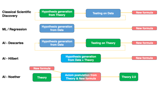
Figure 1: Comparison of AI Noether with other scientific discovery models. While other models are used to discover new formulae, our system analyzes formulae that are not derivable from theory and detects what axioms must be added / changed in order to make the formula derivable.

Abductive reasoning is a field of inference that generates plausible explanations from incomplete observations (peirce1934collected, ; paul1993approaches, ). Unlike deductive reasoning, which obtains a conclusion from a set of premises, abductive reasoning starts with an outcome and ends with a set of plausible explanations, e.g.,

• The fact $C$ is observed.

• If $A$ were true then $C$ would be true.

• There is reason to believe that $A$ is true.

As observed by peirce1934collected , abductive reasoning is arguably “the only logical operation which introduces any new ideas”. Moreover, it is often applied by humans in everyday situations, such as reading between the lines (norvig1987inference, ) and counterfactual reasoning (pearl2002reasoning, ). Doctors use abductive reasoning to propose possible diseases that cause observed symptoms. It has been argued that automating inference may be necessary for understanding and automating consciousness bengio2017consciousness . Yet, abductive reasoning has not yet been incorporated into state-of-the-art AI systems, such as AI-Feynman, AI-Descartes, or AI-Hilbert AI-Feynman ; descartes ; corywright2024evolving . Thus, automating abductive inference is an important component of automating the scientific method.

Our work is related to three parts of the abductive inference and scientific discovery literature: (i) automated abductive inference in logic and more “classical” AI systems, (ii) applications of abductive inference in machine learning, and (iii) machine learning and AI for scientific discovery, as already reviewed in the introduction. Accordingly, we now review the remaining two parts of this literature.

Automated Abductive Inference in Logic and Classical AI:

Marquis marquis proposed automating abductive reasoning in propositional logic and generalized it to first-order logic. Beyond logic, several papers have investigated abductive inference in the context of scientific discovery, e.g., ARROWSMITH for cross-pollinating seemingly unrelated branches of science swanson ; see langley24 for a review of the automation of components of the scientific discovery process, including abductive inference. We follow this line of work in interpreting abduction as the process of selecting or synthesizing hypotheses that complete an incomplete theory in order to explain a target hypothesis.

Automated Abductive Inference for Machine Learning:

The recent surge in popularity of black-box models, including large language models, has led to an interest in explaining the predictions of these models. LIME ribeiro2016 and similar methods provide (local) interpretable explanations that describe the local behavior of any ML model using a weighted linear combination (often sparse) of input features; see rudin2019stop ; lipton2018mythos for reviews of interpretable and explainable machine learning. However, existing works on interpretability and explainability generally focus on computing explanations for black-box models, rather than generating theories that could be used for scientific discovery. In particular, techniques like LIME or SHAP scores cannot, to our knowledge, be leveraged to establish missing axioms in a scientific discovery context.

More recently, a new line of work has explored abductive inference for machine learning dai2019bridging ; ignatiev2019abduction ; zhou2019abductive ; huang2021fast ; yang2024analysis ; see also (wan2024towards, ) for a recent review of this line of work. Initiated by dai2019bridging ; ignatiev2019abduction , the key idea is to embed purely logical reasoning models within the machine learning process to take advantage of the benefits of both machine learning and logical reasoning. For instance, in ignatiev2019abduction , the authors use abductive inference to generate explanations of ML models given input background theories and a set of hypothetical explanations. Moreover, dai2019bridging combines machine learning techniques with a first-order logic model to obtain an output that depends on both models. However, these works do not apply abductive inference to scientific discovery. A comparison of our work to other methods is illustrated in Figure 1.

2 Abductive inference

We assume that all axioms (missing or otherwise) are expressible as polynomial equations of the form $p(x)=0$, and the hypothesis can also be expressed as a polynomial equation. We say that a collection of polynomial equations of the form $p_{1}(x)=0,\ldots,p_{k}(x)=0$ imply the polynomial equation $q(x)=0$ if the latter equation holds for all solutions $\bar{x}$ of the former system of polynomials.

The hypothesis generation step of machine-assisted scientific discovery involves generating a mathematical expression of unknown form that explains potentially noisy data AI-Feynman ; cranmer2023interpretablemachinelearningscience . Recently, the discovery process has been augmented with the use of background axioms that represent a complete, known physical theory, which constrains the space of candidate hypotheses that explain the data descartes ; corywright2024evolving . Data-driven approaches often generate formulae that are not necessarily consistent with theory, while data-theory augmented approaches only return certificates of derivability when background axioms contain sufficient information to explain a hypothesis. In practice, however, theory may be incomplete or inconsistent, and theory needs to be corrected or augmented to explain observational data. We therefore consider the following problem.

Given axioms $A_{1},...,A_{k}$ and a hypothesis $Q$ such that $A_{1},...,A_{k}$ do not imply $Q$, find a set of candidate axioms $A_{k+1},...,A_{r}$ with the “smallest residual” with respect to $A_{1},...,A_{k}$ such that $A_{1},...,A_{r}$ imply $Q$.

Terminology: Throughout the rest of this work, we use the terms $A_{1},\ldots,A_{k}$ “explain” or “imply” $Q$ and $Q$ is a “consequence of” $A_{1},\ldots,A_{k}$ synonymously. Intuitively, the notion of “smallest residual” corresponds to the idea that we wish to add as little new information as possible to $A_{1},\ldots,A_{k}$ to explain $Q$; we will formalize this notion later on. We assume that we do not have data for $A_{k+1},...,A_{r}$; otherwise, the question is equivalent to the hypothesis generation question. We further assume that we do not know what variables $A_{k+1},...,A_{r}$ are defined over, only that they are some subset of all variables in the entire system. Under this setting, our system generates a set of candidate axioms $\{q_{1},...,q_{t}\}$ such that the known axioms along with $q_{i}$ explain $Q$. Further, if no single candidate axiom can be added to explain $Q$, our system detects this. Current machine-assisted discovery tools either rely on partial or complete background theory, or no background theory at all, to discover mathematical expressions that fit observational data, but few append or correct the theory in an automated way, and none do so at the same level of generality.

Example 1.

Assume we have an axiom system defined over 5 real quantities, indicated by $x,y,z,a,b$:

$$x^{2}-ay^{2}=0,$$

$$by-z=0.$$

In this example, we think of $a,b$ as constants in the system (similar in spirit to the Gravitational constant), while $x,y,z$ are quantities that can vary. Let $p_{1}$ be the polynomial $x^{2}-ay^{2}$ and let $p_{2}=by-z$. Thus the axioms are $p_{1}=0$ and $p_{2}=0$. Let

$$q=b^{2}x^{2}-az^{2}.$$

The equation $q=0$ follows from the axioms as

$$q=b^{2}x^{2}-az^{2}=b^{2}(x^{2}-ay^{2})+a(by+z)(by-z)=b^{2}p_{1}+a(by+z)p_{2}.$$ (1)

In the example above, we have expressed $q$ as $\alpha p_{1}+\beta p_{2}$ where $\alpha=b^{2}$ and $\beta=a(by+z)$ are polynomials defined over $x,y,z,a,b$. We say that $q$ is an algebraic combination of the polynomials $p_{1}$ and $p_{2}$ and say that $q=0$ is derivable from $p_{1}=0$ and $p_{2}=0$. As $q=\alpha p_{1}+\beta p_{2}$, it follows that $q=0$ for all values of $x,y,z,a,b$ such that $p_{1}=0$ and $p_{2}=0$. We therefore say that the axioms in the example imply or explain $q=0$.

Table 1: Six minimal theories with two axioms each that explain $q=0$.

$b=0$	$b=0$	$b=0$	$x^{2}-ay^{2}=0$	$x^{2}-ay^{2}=0$	$x^{2}-ay^{2}=0$
$a=0$	$by+z=0$	$by-z$ = 0	$a=0$	$by+z=0$	$by-z=0$

Notice that there are many alternative theories from which the equation $q=0$ follows as a consequence. For example, looking at the equation (1) and letting $p_{3}=by+z$, it is clear that $q=0$ follows from the axioms $p_{1}=0$ and $p_{3}=0$ as $q=\alpha p_{1}+ap_{2}p_{3}$. In a similar manner, we can trivially create the six minimal theories in Table 1 where the first axiom is formed by taking a polynomial that is a factor of $\alpha p_{1}$ and setting it to 0, and the second axiom is similarly composed from a factor of $\beta p_{2}$; $q=0$ is a consequence of each theory.

Each of the 6 axiom systems above is minimal in the sense that we cannot remove an axiom from it and still have $q=0$ as a consequence. Depending on the context, some of the axiom systems may be less interesting than others. For example, if $a$ represents the mass of a pendulum, $a=0$ is likely not an interesting condition. On the other hand, if $a$ represents temperature in Celsius, $a=0$ may represent a meaningful condition.

The axiom system $p_{1}=0,p_{2}p_{3}=0$ is also a valid theory explaining $q=0$, but we call it reducible in the sense that we can trivially get a simpler axiom system if we replace $p_{2}p_{3}$ by either of its factors. Thus, if our only available axioms was $p_{1}=0$, the “residual” of the set of axioms $\{p_{2}p_{3}=0\}$ is not as small as possible. There are other ways of building an infinitude of axiom systems such that $q=0$ is a consequence. Starting from the axiom system $p_{1}=0,p_{2}=0$, it is easy to see that $p_{1}=0,rp_{1}+sp_{2}=0$, where $r,s$ are nonzero real numbers, are valid theories that explain $q=0$. Again, starting with $p_{1}=0$, the axiom set $\{rp_{1}+sp_{2}=0\}$ does not have the least residual.

Now assume we have experimental data for a phenomenon consisting of a number of data points specifying values of $x,z,a,b$ (with $a$ and $b$ unchanging in the data) and assume the data satisfies the equation $b^{2}x^{2}-az^{2}=0$ and that we are able to numerically obtain this equation from the data. Further assume that we have a partial theoretical explanation of the phenomenon, where the partial theory assumes the presence of another variable $y$ and the equation $x^{2}-ay^{2}=0$, i.e., $p_{1}=0$. In this situation, we consider $y$ as an unmeasured quantity, and $x$, $z$, $a$, and $b$ as measured quantities. Given that the data points at hand do not have any values for $y$, it is not possible to infer the relationship $by-z$ directly from the data.

Consider the equation $0=b^{2}p_{1}=b^{2}x^{2}-b^{2}ay^{2}$ that follows from $p_{1}=0$. Subtracting the derived equation $b^{2}x^{2}-az^{2}=0$ from it, we obtain the relationship $a(z^{2}-b^{2}y^{2})=0$ as a consequence of $p_{1}=0$ and $q=0$. This implies that either $a=0$ or $by-z=0$ or $by+z=0$. Each of the equations (or products of pairs of equations) in the previous line can be appended to $p_{1}=0$ to get a valid theory (in the absence of other information) explaining $q=0$.

Using the notation above, “derivable from” implies “can be explained by”. We will later discuss conditions under which the converse is true.

2.1 Method

Our goal is to identify a candidate missing polynomial axiom $A_{k+1}$ that, along with a known set of axioms $A_{1},\ldots,A_{k}$, can be used to derive a target hypothesis $Q$. The method consists of three main steps—Encode, Decompose, and Reason—illustrated in Figure 2 and summarized in the  Algorithm Summary.

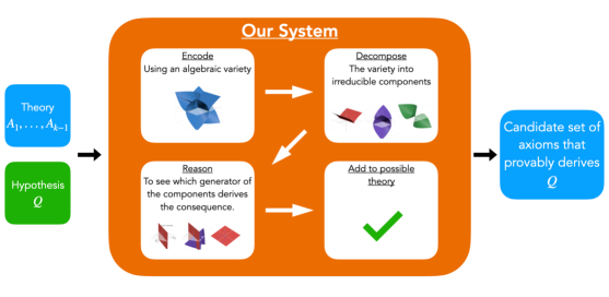
Figure 2: AI Noether: Encode—form $I=\langle A_{1},\dots,A_{k},Q\rangle$; Decompose—primary decomposition with primes $P_{j}$; Reason—test generators $g\in P_{j}$ by augmenting and eliminating to $\mathrm{vars}(Q)$; passing $g$ are candidate $A_{k+1}$.

Encode. Given a collection of known axioms $A_{1},\ldots,A_{k}$ and a hypothesis $Q$, we form the solution set of the system $\{A_{1},\ldots,A_{k},Q\}$. Each equation defines a hypersurface in $\mathbb{R}^{n}$, and the intersection of these hypersurfaces defines a geometric object—referred to as the variety of the system. We will use this geometric perspective to recast the ideas of $Q$ being derivable from $A_{1},...A_{k}$ as well as $Q$ being derivable from some larger set of axioms $A_{1},...,A_{k+r}$ as geometric manipulations.

Decompose. The set of solutions (variety) of the equation $xy=0$ (where $x$ and $y$ are real variables) is not irreducible - i.e., that is, it is the union of two smaller solution sets (varieties), i.e., solutions of $x=0$ and of $y=0$. We similarly decompose the solution set of the system $\{A_{1},\ldots,A_{k},Q\}$ into smaller components representing minimal geometric subsets (with some properties that will be made precise shortly) that cannot be decomposed further, illustrated in Figure 3. When $Q$ is not a consequence of the axioms (and thus not derivable from the axioms), some components in the variety of $\{A_{1},\ldots,A_{k},Q\}$ will not be present in the variety of $\{A_{1},\ldots,A_{k}\}$. These residual components capture algebraic constraints that make $Q$ hold locally but are not globally entailed by the axioms. For example, if $Q=\alpha_{1}A_{1}+\cdots+\alpha_{k+1}A_{k+1}$ for unknown coefficients but $A_{k+1}$ is missing, then the solution set may decompose into components corresponding to the missing axiom. Decomposition isolates these structures.

Figure 3: Geometric visualization of decomposition - On the left, we have an example of a variety which is the solution to a system of polynomial equations. The middle and right show that this variety can be decomposed into irreducible components, which geometrically is the process of finding smaller varieties whose union is the original variety.

Reason. For each irreducible component, we extract its defining polynomials and test whether any subset, when added to the axioms, is sufficient to derive $Q$. This is done by forming the solution set of $\{A_{1},\ldots,A_{k}\}\cup\{g\}$ for a candidate polynomial $g$, and projecting it onto the variables appearing in $Q$, illustrated in Figure 4. If this projection lies within the solution set of $Q$, then $Q$ is implied by the augmented system. Such $g$ are returned as candidate missing axioms. If no such $g$ exists, we conclude that no single missing axiom explains $Q$.

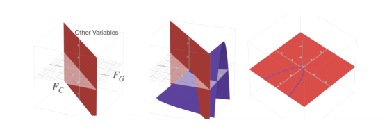
Figure 4: Geometric visualization of reasoning. On the left, we have some surface defined by an axiom (here, $F_{c}=F_{g}$ as an example). In the middle, we have an additional equation which defines a new surface. In order to apply the axiom to the new surface, we project the surface onto the space defined by the known axiom(s).

Algorithm 1 Algorithm Summary

1:Input: Axioms $A_{1},\ldots,A_{k}$ and hypothesis $Q$

2:Encode: Construct the solution set of $\{A_{1},\ldots,A_{k},Q\}$

3:Decompose: Break the solution set into irreducible components

4:for each component do

• Extract defining polynomials (also called generators)

• Reason: Test whether adding any generator allows $Q$ to be derived from the axioms

5:end for

6:Output: Set of candidate missing axioms sufficient to explain $Q$

This method does not require access to data for the missing axiom or prior knowledge of the variables it depends on. It returns a set of explanatory candidates when possible, or certifies failure when no such single axiom exists. We develop the algebraic details in the following section.

2.2 Preliminaries

We define notions specific to real algebraic geometry; see Cox+Others/1991/Ideals for further details. Let $\mathbb{R}$ denote the set of real numbers and let $R=\mathbb{R}[x_{1},...,x_{n}]$ be the ring of polynomials defined over the $n$ variables $x_{1},\ldots,x_{n}$ with real coefficients. Axioms and hypotheses in our model will be equations of the form $p(x)=0$ where $p\in R$. We abuse notation and identify an axiom by its defining polynomial. We will focus on real-valued solutions of axiom systems; see the appendix for more details.

Encode. An ideal over $R$ is a subset $I$ of $R$ that is closed under addition and also multiplication by elements of $R$: if $f,g\in I$, then $f+g\in I$ and $\alpha f\in I$ for any $\alpha\in R$. Given polynomials $A_{1},...,A_{k}\in R$, we denote the set of all algebraic combinations of $A_{1},\ldots,A_{k}$ by

$$\langle A_{1},\ldots,A_{k}\rangle=\{f\in R:f=\sum_{i=1}^{k}\alpha_{i}A_{i}\text{ for some }\alpha_{i}\in R\}.$$

called an ideal over $R$ with generators $A_{1},\ldots,A_{k}$. Let $\mathcal{A}$ stand for $\{A_{1},\ldots,A_{k}\}$, and let $I(\mathcal{A})$ stand for the ideal $\langle A_{1},\ldots,A_{k}\rangle$. Our earlier notion of “derivability” corresponds to ideal membership: $Q=0$ is derivable from $\mathcal{A}$ if $Q$ is an algebraic combination of $A_{1},\ldots,A_{k}$, i.e., if $Q\in I(\mathcal{A})$. Given an ideal $I$, we define the variety of $I$, denoted $V(I)$, as the set

$$V(I)=\{\mathbf{x}\in\mathbb{R}^{n}:A_{i}(\mathbf{x})=0\text{ for each }A_{i}\in I\}.$$

A standard fact from algebraic geometry is that the set above is the same as the solution set to any finite collection of polynomials that generate the same ideal. Encoding equations with ideals and varieties has a key advantage in that it allows us to study logical implication and consistency questions geometrically: if $Q=0$ can be derived from $A_{1}=0,\ldots,A_{k}=0$, then $V(A_{1},\ldots,A_{k},Q)=V(A_{1},\ldots,A_{k})$. If adding $Q$ to $\mathcal{A}$ introduces extra structure into the resulting variety, then $Q$ is not derivable from $\mathcal{A}$.

Decompose. Assume $Q$ is not implied by $\mathcal{A}$. Then $V(\mathcal{A},Q)\neq V(\mathcal{A})$. Suppose $Q$ can be derived nontrivially from an axiom $A_{k+1}$ along with $\mathcal{A}$, i.e., $Q=\alpha_{1}A_{1}+\cdots\alpha_{k+1}A_{k+1}$ for some polynomials $\alpha_{i}$ without $\alpha_{k+1}=1,A_{k+1}=Q$. In this case $V(A_{1},...A_{k},Q)=V(A_{1},...,A_{k},\alpha_{k+1}A_{k+1})$ and since $\alpha_{k+1}\neq 1$, we know that intersecting $V(Q)$ with $V(\mathcal{A})$ is the same as intersecting $V(\alpha_{k+1}A_{k+1})$ with $V(\mathcal{A})$. Since $V(\alpha_{k+1}A_{k+1})$ is reducible, we are introducing new reducibility into $V(\mathcal{A})$ that is a factor of the residual $\alpha_{k+1}A_{k+1}=Q-(\sum_{i=1}^{k}\alpha_{i}A_{i})$. We therefore can take our intersected variety $V(\mathcal{A},Q)$ and study its irreducible components. We next define the mechanisms required for this process.

A prime ideal is an ideal $P\subset R$ such that if $fg\in P$ with $f,g\in R$, then $f\in P$ or $g\in P$.

For a prime ideal $P$, $V(P)$ is irreducible, i.e., it cannot be represented as the union of two proper subsets that are varieties. The radical of an ideal $I$ is denoted by $\sqrt{I}$ and is defined as:

$$\sqrt{I}=\{f\in R:f^{m}\in I\text{ for some positive integer }m\}.$$

The following key theorem allows us to break up a variety into irreducible components:

Theorem 1 (Primary Decomposition).

Any ideal $I$ can be decomposed into an intersection of ideals

$$I=Q_{1}\cap...\cap Q_{r}$$

such that

1. There are no redundancies among the $Q_{i}$, i.e., for each $j$ we have $\cap_{i\neq j}Q_{i}\not\subset Q_{j}$.

2. For each $i$, $\sqrt{Q_{i}}$ is a prime ideal (called an associated prime of $I$).

Let $P_{i}=\sqrt{Q_{i}}$. Using the fact that for any ideals $I,J$, we have $V(I\cap J)=V(I)\cup V(J)$ and $V(I)=V(\sqrt{I})$ Cox+Others/1991/Ideals , we get from the primary decomposition that a variety can be decomposed into a union of varieties corresponding to prime ideals: $V(I)=\bigcup_{i=1}^{r}V(P_{i})$.

Decomposition in this setting serves a role analogous to Principal Component Analysis (PCA) in linear algebra, identifying latent, independent substructures that explain variation in the system. Whereas PCA decomposes a dataset into orthogonal directions of variance, primary decomposition identifies algebraically independent pieces of a solution space introduced by inconsistency or incompleteness.

Reason. Finally, for derivability, we need to define the algebraic notion of eliminating indeterminates from a system of polynomials. A “reduced Gröbner basis” of an ideal $I\subset R$ is a unique generating set $\{G_{1},\ldots,G_{m}\}$ that satisfies $\langle G_{1},...,G_{m}\rangle=\langle A_{1},...,A_{k}\rangle=I$. If we define a lexicographic ordering $x_{1}>...>x_{n}$ on the indeterminates and compute the associated reduced Gröbner basis, then we have the following property.

Theorem 2 (Elimination Theorem).

For any integer $d$ with $1\leq d\leq n$, $\langle\{G_{1},...,G_{m}\}\cap\mathbb{R}[x_{1},...,x_{d}]\rangle=\langle A_{1},....,A_{k}\rangle\cap\mathbb{R}[x_{1},...,x_{d}]$

So if we want to eliminate the variables $x_{d+1},...,x_{n}$ from the system, i.e., compute the ideal $\langle A_{1},...,A_{k}\rangle\cap\mathbb{R}[x_{1},...,x_{d}]$ which has infinitely many polynomials, we can compute a set of generators by finding a Gröbner basis of $I$ and considering the elements defined over the variables $x_{1},\ldots,x_{d}$. Geometrically, this corresponds to taking the variety in $n$-dimensional real space $V(I)$ and finding the projection $\pi_{d}V(I)=V(I\cap\mathbb{R}[x_{1},...,x_{d}])\subset\mathbb{R}^{d}$ into the $d$-dimensional real space defined over the remaining variables. This provides a way to test algebraic consequence: if $Q$ depends only on variables $x_{1},\ldots,x_{d}$, we can eliminate all other variables and check whether $Q$ is present in the projected ideal. We use this to test whether $Q$ can be derived from a set of axioms and a candidate additional axiom extracted from decomposition. If so, we return the candidate as a possible missing axiom. While eliminating the variables is not strictly necessary to test for membership in the ideal, it allows for the stronger elimination of trivial axiom candidates that project onto smaller trivial surfaces that represent undesired conditions under which $Q$ can be derived.

We will address necessary and sufficient conditions required for axiom recovery in section 3.3.1. The generalized algorithm is detailed in Algorithm 1 in Appendix 6

3 Results

In this section, we present the results from testing our system on various real-world physical theories. We test our ideas on $10$ systems reported in AI Hilbert corywright2024evolving as well as another appearing in a recent paper phothall .

3.1 Problem 1. Kepler’s Third Law

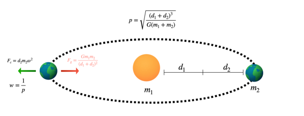
Figure 5: AI Noether detects the existence of gravitational force, an essential axiom required to derive Kepler’s third law.

Setting. Consider Kepler’s third law, which relates the orbital period of two celestial bodies to their distances and masses. It can be written as

$$Q:=p-2\pi\sqrt{\frac{(d_{1}+d_{2})^{3}}{G(m_{1}+m_{2})}}=0,$$

where $p$ is the orbital period, $m_{1},m_{2}$ the masses, and $d_{1},d_{2}$ their distances from the center of mass. For circular orbits, we use the following axioms (with $p$ scaled so that $\omega p=1$):

$$A_{1} :(d_{1}+d_{2})^{2}F_{g}-Gm_{1}m_{2}=0$$ (2)

$$A_{2} :F_{c}-m_{2}d_{2}\omega^{2}=0$$ (3)

$$A_{3} :F_{g}-F_{c}=0$$ (4)

$$A_{4} :\omega p-1=0$$ (5)

$$A_{5} :m_{1}d_{1}-m_{2}d_{2}=0.$$ (6)

Equation (2) gives gravitational force, (3) centrifugal force, (4) equates them, (5) relates frequency and period, and (6) defines the center of mass. To derive $Q$, we eliminate $d_{1}$ using (6), substitute $p=1/\omega$ from (5), and replace $\omega^{2}$ by combining (3)–(4) with (2). This yields

$$G(m_{1}+m_{2})p^{2}-(d_{1}+d_{2})^{3}=0,$$

which is Kepler’s law in polynomial form. Equivalently, setting

$$\alpha_{1}=-p^{2},\ \ \alpha_{2}=p^{2}(d_{1}+d_{2})^{2},\ \ \alpha_{3}=-p^{2}(d_{1}+d_{2})^{2},\ \ \alpha_{4}=m_{2}d_{2}(\omega p+1)(d_{1}+d_{2})^{2},\ \ \alpha_{5}=-d_{2}^{2},$$

we obtain

$$Q=\alpha_{1}A_{1}+\alpha_{2}A_{2}+\alpha_{3}A_{3}+\alpha_{4}A_{4}+\alpha_{5}A_{5}.$$

Our System Now assume that we are missing knowledge of the equation of gravitational force – axiom $A_{1}$ – but we have Kepler’s law $Q$ at hand (possibly derived from sufficient data; see AI-Feynman ; descartes ; corywright2024evolving ). At this point, not only $A_{1}$ but also $\alpha_{1},\ldots,\alpha_{5}$ are not known. We will assume they exist and attempt to find them from $Q$ and the remaining known axioms $A_{2}-A_{5}$. Here we view $\alpha_{1}A_{1}$ as the (unknown) residual of $Q$ with respect to $A_{2},\ldots,A_{5}$. We define the ideal $I=\langle A_{2},A_{3},A_{4},A_{5},Q\rangle$. This is the same as the ideal $\langle A_{2},A_{3},A_{4},A_{5},\alpha_{1}A_{1}\rangle$ as $Q=\sum_{i=1}^{5}\alpha_{i}A_{i}$. Geometrically, $V(A_{2},A_{3},A_{4},A_{5},\alpha_{1}A_{1})=V(A_{2},A_{3},A_{4},A_{5})\cap V(\alpha_{1}A_{1})$. Since the latter is reducible, we have more irreducible components than we have for $V(A_{2},A_{3},A_{4},A_{5})$. Computing a primary decomposition of $I$ then gives us the following associated primes:

Decomposition

Variety 1 $\langle d_{2},\;m_{1},\;F_{g},\;F_{c},\;wp-1\rangle$

Variety 2 $\langle m_{2},\;d_{1},\;F_{g},\;F_{c},\;wp-1\rangle$

Variety 3 $\langle m_{2},\;m_{1},\;F_{g},\;F_{c},\;wp-1\rangle$

Variety 4 $\begin{aligned} \mathopen{\langle}\;&F_{c}-F_{g},\;m_{1}d_{1}-m_{2}d_{2},\;wp-1,\;F_{g}p-wm_{2}d_{2},\;F_{g}p^{2}-m_{2}d_{2},\\ &\hbox{\pagecolor{BrickRed!10}$\color[rgb]{0,0,0}\mathbf{F_{g}(d_{1}+d_{2})^{2}-m_{1}m_{2}G}$},\;d_{1}(d_{1}+d_{2})^{2}-m_{2}p^{2}G,\;m_{1}p^{2}G-d_{2}(d_{1}+d_{2})^{2},\\ &wd_{1}^{2}(d_{1}+d_{2})^{2}-m_{1}pG,\;wd_{1}^{3}-3wd_{1}d_{2}^{2}-2wd_{2}^{3}+2m_{1}pG-m_{2}pG\;\mathclose{\rangle}\end{aligned}$

Generators selected by Reasoning module

$\color[rgb]{0,0,0}\mathbf{F_{g}(d_{1}+d_{2})^{2}-m_{1}m_{2}G}$

The generators of these irreducible components/ideals represent key equations that define each irreducible component. We iterate through each generator $\hat{A_{1}}$ and compute a Gröbner basis to eliminate the variables not appearing in $Q$. We find that only the correct expression - $\color[rgb]{0,0,0}\mathbf{F_{g}(d_{1}+d_{2})^{2}-m_{1}m_{2}G}$ - can derive $Q$ and is therefore the only candidate returned by our system.

Axiom Formatting and Multipliers. Since the reducibility is introduced by $V(\alpha_{i}A_{i})$, we do not distinguish between $\alpha_{i}$ and $A_{i}$ when searching for $i$th axiom candidates. Additionally, we might return axioms in alternate forms - the exact expression is not guaranteed. For example, consider the same Kepler axioms and assume we are missing axiom $A_{4}$ instead. Then the relevant ideals in the primary decomposition are:

Decomposition

Variety 1 $\begin{aligned} \mathopen{\langle}\;F_{c}-F_{g},\;m_{1}d_{1}-m_{2}d_{2},\;\hbox{\pagecolor{BrickRed!10}$\color[rgb]{0,0,0}\mathbf{wp-1}$},\;F_{g}p-wm_{2}d_{2},\;\hbox{\pagecolor{BrickRed!10}$\color[rgb]{0,0,0}\mathbf{F_{g}p^{2}-m_{2}d_{2}}$},\\ \qquad F_{g}(d_{1}{+}d_{2})^{2}-m_{1}m_{2}G,\;d_{1}(d_{1}{+}d_{2})^{2}-m_{2}p^{2}G,\\ \qquad m_{1}p^{2}G-d_{2}(d_{1}{+}d_{2})^{2},\;w\,d_{2}(d_{1}{+}d_{2})^{2}-m_{1}pG,\\ \qquad w(d_{1}-2d_{2})(d_{1}{+}d_{2})^{2}+2m_{1}pG-m_{2}pG\;\mathclose{\rangle}\end{aligned}$

Variety 2 $\begin{aligned} \mathopen{\langle}\;F_{c}-F_{g},\;m_{1}d_{1}-m_{2}d_{2},\;\hbox{\pagecolor{BrickRed!10}$\color[rgb]{0,0,0}\mathbf{wp+1}$},\;F_{g}p+wm_{2}d_{2},\;F_{g}p^{2}-m_{2}d_{2},\\ \qquad F_{g}(d_{1}{+}d_{2})^{2}-m_{1}m_{2}G,\;d_{1}(d_{1}{+}d_{2})^{2}-m_{2}p^{2}G,\\ \qquad m_{1}p^{2}G-d_{2}(d_{1}{+}d_{2})^{2},\;w\,d_{2}(d_{1}{+}d_{2})^{2}+m_{1}pG,\\ \qquad w(d_{1}-2d_{2})(d_{1}{+}d_{2})^{2}-2m_{1}pG+m_{2}pG\;\mathclose{\rangle}\end{aligned}$

Generators selected by Reasoning module

$\color[rgb]{0,0,0}\mathbf{wp-1}$

$\color[rgb]{0,0,0}\mathbf{F_{g}p^{2}-m_{2}d_{2}}$

$\color[rgb]{0,0,0}\mathbf{wp+1}$

The highlighted polynomials are returned by our system as being axiom candidates that derive $Q$ along with the remaining axioms. The other generators have been omitted for readability, and cannot derive $Q$. While the correct expression $wp-1$ is present, we have additional terms. The term $F_{g}p^{2}-m_{2}d_{2}$ is a restatement of $A_{2}$ using $A_{3}$ and the unknown $wp-1$ substituted in. It contains the same information as $wp-1$ since the former is already known. The term $wp+1$ is an artifact of the fact that $\alpha_{4}$ as noted before is $m_{2}d_{2}(wp+1)(d_{1}+d_{2})^{2}$. Note that the variety $V(m_{2}d_{2}(wp+1)(d_{1}+d_{2})^{2})$ is reducible and can be written as the union: $V(m_{2})\cup V(d_{2})\cup V(wp+1)\cup V((d_{1}+d_{2})^{2})$. Therefore, $wp+1$ appears as a viable axiom candidate since there is an algebraic derivation of $Q$ from the remaining axioms along with $wp+1$. Incidentally, the remaining terms $m_{2}$, $d_{2}$, and $(d_{1}+d_{2})^{2}$ also show up in the associated primes:

Decomposition

Variety 1 $\begin{aligned} \mathopen{\langle}\;F_{c}-F_{g},\;m_{2}^{2},\;\hbox{\pagecolor{BrickRed!10}$\color[rgb]{0,0,0}\mathbf{(d_{1}{+}d_{2})^{2}}$},\;m_{1}d_{2}+d_{1}m_{2}+2m_{2}d_{2},\;m_{1}m_{2},\\ \qquad m_{1}d_{1}-m_{2}d_{2},\;m_{1}^{2},\;F_{g}m_{2},\;F_{g}m_{1},\;F_{g}^{2},\;F_{g}-w^{2}m_{2}d_{2}\;\mathclose{\rangle}\end{aligned}$

Variety 2 $\langle\hbox{\pagecolor{BrickRed!10}$\color[rgb]{0,0,0}\mathbf{d_{2}}$},\;m_{1},\;F_{g},\;F_{c}\rangle$

Variety 3 $\langle\hbox{\pagecolor{BrickRed!10}$\color[rgb]{0,0,0}\mathbf{m_{2}}$},\;d_{1},\;F_{g},\;F_{c}\rangle$

Generators selected by Reasoning module

$\color[rgb]{0,0,0}\mathbf{(d_{1}{+}d_{2})^{2}}$

$\color[rgb]{0,0,0}\mathbf{d_{2}}$

$\color[rgb]{0,0,0}\mathbf{m_{2}}$

Applying the elimination theorem and keeping only the candidates that project exactly onto the variables over which $Q$ is defined eliminates these candidates.

3.2 Single Axiom Removed Results

Problem	# Axioms Recovered	Avg. Time (s)	Total Axioms
Kepler	5/5	0.1	5
Compton	10/10	5.4	10
Einstein	5/5	1.5	5
Escape Velocity	5/5	0.4	5
Light Damping	5/5	1.6	5
Hagen Poiseuille	4/4	0.6	4
Neutrino Decay	5/5	3.5	5
Hall Effect	7/7	11.1	9
Carrier-Resolved Photo-Hall Effect	7/7	1.1	7

Table 2: Summary of Axiom Recovery Performance by Problem

We tested our system on 7 axiom systems from AI Hilbert, as well as on a more recent work in the scientific literature phothall . In each case, We iterate through the axioms, drop an axiom from the system, and test if we can recover the missing axiom while not making any assumption about it. In almost every case, we were able to recover the missing axiom. A detailed list of axioms in each system can be found in the Appendix 5.4.

3.3 Multiple missing axioms

We demonstrated efficacy in removing/correcting one axiom from an axiom list. We now look at what happens when we need to recover more than one axiom in order to explain a hypothesis $Q$. In this case, we have

$$Q=\sum_{i=1}^{k}\alpha_{i}A_{i}$$

but we only have access to $A_{1},...,A_{k-r}$. Alternatively, we want to find a substitution for $r$ axioms in our system in order to explain $Q$.

Kepler’s Third Law of Planetary Motion

Recall that the Kepler axioms were:

$$A_{1}:=(d_{1}+d_{2})^{2}F_{g}-Gm_{1}m_{2}$$ (7)

$$A_{2}:=F_{c}-m_{2}d_{2}w^{2}$$ (8)

$$A_{3}:=F_{g}-F_{c}$$ (9)

$$A_{4}:=wp-1$$ (10)

$$A_{5}:=m_{1}d_{1}-m_{2}d_{2}$$ (11)

The statement of Kepler’s law is:

$$Q:=m_{1}m_{2}Gp^{2}-d_{2}^{2}d_{1}m_{1}-d_{1}^{2}d_{2}m_{2}-2d_{1}d_{2}^{2}m_{2}-d_{1}^{2}d_{2}m_{2}$$ (12)

Assume that we are missing axioms (9) and (10) - the relationship between centrifugal and gravitational force and the relationship between frequency and period. Then, encoding the known information - equations (7), (8),(11), and (12) - our system returns the following relevant component of the primary decomposition and selected generator from the reasoning module:

Selected varieties from Decomposition module

Variety 1 $\begin{aligned} \mathopen{\langle}\;m_{1}d_{1}-m_{2}d_{2},\;\hbox{\pagecolor{BrickRed!10}$\color[rgb]{0,0,0}\mathbf{F_{g}p^{2}-m_{2}d_{2}}$},\;F_{g}(d_{1}^{2}+2d_{1}d_{2}+d_{2}^{2})-m_{1}m_{2}G,\\ \qquad d_{1}^{3}+2d_{1}^{2}d_{2}+d_{1}d_{2}^{2}-m_{2}p^{2}G,\;m_{1}p^{2}G-d_{1}^{2}d_{2}-2d_{1}d_{2}^{2}-d_{2}^{3},\\ \qquad F_{c}-w^{2}m_{2}d_{2},\;F_{c}p^{2}G-w^{2}d_{1}^{3}d_{2}-2w^{2}d_{1}^{2}d_{2}^{2}-w^{2}d_{1}d_{2}^{3}\;\mathclose{\rangle}\end{aligned}$

Generators selected by Reasoning module

$\color[rgb]{0,0,0}\mathbf{F_{g}p^{2}-m_{2}d_{2}}$

We therefore return $\color[rgb]{0,0,0}\mathbf{F_{g}p^{2}-m_{2}d_{2}}$. This equation is the same as the centrifugal force equation (8) but with the missing relationships $F_{c}=F_{g}$ and $w=\frac{1}{p}$ substituted in. Therefore, the missing information is discovered, since equation (8) is assumed to be known, although it is not decoupled. To go one step further, we can remove three out of the five axioms: equations (8),(9), and (10), leaving us with only the gravitational force equation (7) and center of mass equation (11). Similarly, running our system with the Kepler hypothesis gives us a similar component:

Selected varieties from Decomposition module

Variety 1 $\begin{aligned} \mathopen{\langle}\;m_{1}d_{1}-m_{2}d_{2},\;\hbox{\pagecolor{BrickRed!10}$\color[rgb]{0,0,0}\mathbf{F_{g}p^{2}-m_{2}d_{2}}$},\;F_{g}(d_{1}^{2}+2d_{1}d_{2}+d_{2}^{2})-m_{1}m_{2}G,\\ \qquad d_{1}^{3}+2d_{1}^{2}d_{2}+d_{1}d_{2}^{2}-m_{2}p^{2}G,\;m_{1}p^{2}G-d_{1}^{2}d_{2}-2d_{1}d_{2}^{2}-d_{2}^{3}\;\mathclose{\rangle}\end{aligned}$

Generators selected by Reasoning module

$\color[rgb]{0,0,0}\mathbf{F_{g}p^{2}-m_{2}d_{2}}$

We get the same axiom candidate. However, in the previous case, where we had knowledge of the centrifugal force equation, we are assuming here that we do not know it. So we’re not only recovering the relationships $F_{c}=F_{g}$ and $wp-1$, but also the centrifugal force axiom itself $F_{c}=m_{2}d_{2}w^{2}$ with the former relations coupled with it.

Table 3 shows the results of attempting to recover various combinations of pairs and triples of axioms for Kepler’s third law.

Problem	Missing Axioms	Recovered	Recovered Axiom(s)
Kepler	$\{\texttt{G},\texttt{cf}\}$	X	–
Kepler	$\{\texttt{G},\texttt{C}\}$		$(d_{1}+d_{2})^{2}F_{c}=Gm_{1}m_{2}$
Kepler	$\{\texttt{G},\texttt{wp}\}$	X	–
Kepler	$\{\texttt{cf},\texttt{C}\}$		gravitational force
Kepler	$\{\texttt{cf},\texttt{wp}\}$		gravitational force
Kepler	$\{\texttt{C},\texttt{wp}\}$		gravitational force
Kepler	$\{\texttt{G},\texttt{cf},\texttt{C}\}$	X	–
Kepler	$\{\texttt{G},\texttt{cf},\texttt{wp}\}$	X	–
Kepler	$\{\texttt{G},\texttt{C},\texttt{wp}\}$	X	–
Kepler	$\{\texttt{cf},\texttt{C},\texttt{wp}\}$		gravitational force

Table 3: Recovery results on the Kepler problem for various subsets of missing axioms. Shorthand: G = gravitational force $(d_{1}+d_{2})^{2}F_{g}=Gm_{1}m_{2}$, cf = centrifugal force $F_{c}=m_{2}d_{2}w^{2}$, C = force balance $F_{g}=F_{c}$, wp = frequency-period relation $wp=1$, cm = center of mass $m_{1}d_{1}=m_{2}d_{2}$.

Across six benchmark systems, we removed pairs and triples of axioms and attempted to recover explanations for $Q$. Success rates range from 25–60% (Kepler 5/10; Hagen–Poiseuille 6/10; Einstein 8/20; others 5–7/20), with most failures occurring when three axioms are missing, especially in larger axiom sets. Runtimes are modest overall (avg. 0.1–3.5 s), with heavier systems (Einstein, Neutrino Decay) taking longer on average. The results can be seen in table 4.

Problem	# Tuples Recovered	Avg. Time (s)	# of Axioms
Kepler	5/10	0.1	4
Einstein	8/20	1.5	5
Escape Velocity	6/20	0.4	5
Light Damping	5/20	1.6	5
Hagen Poiseuille	6/10	0.6	4
Neutrino Decay	7/20	3.5	5

Table 4: Summary of 2- and 3-Axiom Tuple Recovery Performance by Problem

3.3.1 Criteria for Recoverability of Axioms

The theorem below provides a sufficient criterion for recovering missing axioms.

First we will need the notion of height of an ideal. For a prime ideal $P$, we define its height, $\operatorname{ht}(P)$, as the length $n$ of the longest chain $P_{0}\subsetneq P_{1}\cdots\subsetneq P_{n}=P$ of prime ideals contained in $P$. For a general ideal, its height is the minimum of the heights of its associated primes, which is the same as the minimum of the heights of all primes which contain the ideal.

Theorem 3 (Common minimal associated prime).

Given ideals $I\subset J\subsetneq\mathbb{R}[x_{1},...,x_{n}]\;|\;\operatorname{ht}(I)=\operatorname{ht}(J)$, then $I$ and $J$ have a common minimal associated prime.

Proof. Let $P$ be an associated prime for $J$ such that $\operatorname{ht}(P)=\operatorname{ht}(J)$. Then we have that $I\subset J\subset P$. Since $\operatorname{ht}(I)=\operatorname{ht}(P)$, there is no prime $Q$ such that $I\subset Q\subsetneq P$. Otherwise $\operatorname{ht}(I)\leq\operatorname{ht}(Q)<\operatorname{ht}(P)$. But then $P$ is a minimal prime containing $I$ and thus a minimal associated prime for $I$.

Consider $I$ to be the ideal with known information $\langle A_{1},...,A_{k},Q\rangle$ and $J$ the ideal of the true axioms $\langle A_{1},...,A_{k+1}\rangle$. If $I$ and $J$ have the same height, then we know that they have a common associated prime, which contains the missing axiom $A_{k+1}$. If $Q$ and $A_{k+1}$ are not contained in any of the associated primes for $\langle A_{1},...,A_{k}\rangle$, then we have that $\operatorname{ht}\langle A_{1},...,A_{k},Q\rangle=\operatorname{ht}\langle A_{1},...,A_{k+1}\rangle$ and the theorem applies.

Typically if multiple axioms are missing, adding back a single phenomenon $Q$, will not be sufficient, so in general we will need to add back several consequent phenomena $\{Q_{1},\ldots Q_{h}\}$ in order to generate an ideal which is guaranteed to have a component which contains all the missing axioms.

Our missing axiom construction is attempting to find axioms which are sufficient to derive $Q$, i.e. whether or not $Q$ is contained in the ideal generated by the axioms. If we want to decide whether or not a set of axioms implies $Q$, given the ideal $I$ generated by the axioms, we are asking whether $V(I)\subset V(Q)$. To make this test effective, we need to construct the biggest ideal with the same set of zeros, this is $I(V(I))$. So the test whether a set of axioms $A$ implies $Q$ is whether $Q\in I(V\langle A\rangle)$. If our varieties are defined over the reals, then $I(V\langle A\rangle)$ can be computed as the real radical of the ideal $\langle A\rangle$.

4 Conclusion and Remarks

In this work, we propose an AI system called AI-Noether, which bridges the gap between AI-driven scientific discoveries and existing scientific knowledge, provided both the discoveries and the knowledge are expressible as real polynomials. In particular, given a set of background theory axioms and a discovered polynomial, our approach derives a minimal set of additional polynomial axioms necessary to derive the given polynomial. Furthermore, we demonstrate the effectiveness of our approach on a selection of renowned scientific laws, including Kepler’s Third Law and the Carrier-Resolved Photo-hall effect.

For future work, it would be interesting to extend our approach to settings with non-polynomial scientific laws, e.g., settings where laws are expressed as ODEs or PDEs. It would also be interesting to apply our approach to new data-driven scientific discoveries, thereby reconciling them with prior literature.

5 Appendix

5.1 Differences between real and complex solutions

Let $A_{1},\ldots,A_{k}$ be a collection of polynomials with $A_{1}=0,\ldots,A_{k}=0$ being the associated axioms. Let $\mathcal{A}$ stand for the set $\{A_{1},\ldots,A_{k}\}$. Let $V_{R}(\mathcal{A})$, respectively $V_{C}(\mathcal{A})$, be the set of real, respectively complex, solutions of the equations $A_{1}=0,\ldots,A_{k}=0$. Note that $V_{R}(\mathcal{A})$ is the same as the variety $V(\mathcal{A})$ defined in the main body of the paper.

First note that $V_{C}(\mathcal{A},Q)=V_{C}(\mathcal{A})$ if and only if $Q=0$ for all complex solutions of $A_{1}=0,\ldots,A_{k}=0$. Further, if $Q\in I(\mathcal{A})$, then $V_{C}(\mathcal{A},Q)=V_{C}(\mathcal{A})$. However, the converse is not true. By Hilbert’s Nullstellensatz, if $V_{C}(\mathcal{A},Q)=V_{C}(\mathcal{A})$, then $Q^{m}\in I(\mathcal{A})$ for some positive integer $m$ (but $m$ need not equal 1). But $Q^{m}(\bar{x})=0$ if and only $Q(\bar{x})=0$. Accordingly, if we say that $Q=0$ is derivable from $\mathcal{A}$ if and only if $Q^{m}\in I(\mathcal{A})$, then the notions of “a consequence of” and “derivable from” are identical assuming complex-valued solutions are relevant.

On the other hand, if we are only interested in real-valued solutions, the situation is more complicated. As before, $V_{R}(\mathcal{A},Q)=V_{R}(\mathcal{A})$ if and only if $Q=0$ for all real solutions of $A_{1}=0,\ldots,A_{k}=0$. Further, if $Q\in I(\mathcal{A})$, then $V_{R}(\mathcal{A},Q)=V_{R}(\mathcal{A})$. However, the converse is not true. If $V_{R}(\mathcal{A},Q)=V_{R}(\mathcal{A})$, then $Q^{2m}+S\in I(\mathcal{A})$ for some positive integer $m$ and some polynomial $S$ that is a sum of squares of polynomials in $R$.

5.2 Problem 2. Einstein’s Relativistic Time Dilation Law

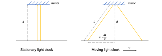
Figure 6: Moving clock experiment for obtaining Einstein’s time dilation formula.

Einstein’s time dilation law describes how two observers in motion experience time differently. Letting $c$ be the speed of light, $f$ the frequency of a clock moving at speed $v$, and $f_{0}$ the frequency of a stationary clock, illustrated in Figure 6, we have the relation:

$$\frac{f}{f_{0}}=\sqrt{1-\frac{v^{2}}{c^{2}}}$$

which, after squaring and clearing denominators, gets us:

$$c^{2}f_{0}^{2}-c^{2}f^{2}-f_{0}^{2}v^{2}=0$$ (13)

This can be derived from the following axioms:

$$A_{1}:=cdt_{0}-2d=0$$ (14)

$$A_{2}:=cdt-2L=0$$ (15)

$$A_{3}:=4L^{2}-4d^{2}-v^{2}\,dt^{2}=0$$ (16)

$$f_{0}dt_{0}-1=0$$ (17)

$$fdt-1=0$$ (18)

$A_{1}$ encodes the time taken for light to travel from a stationary light source and be reflected back to the origin from a stationary mirror. $A_{2}$ similarly captures the time taken for light to start from a moving light-source and arrive back at the source (at its new position) after reflection in a stationary mirror. $A_{3}$ relates the initial distance between the light-source and mirror to the distance traveled by light because of the motion. $A_{4},A_{5}$ relate frequencies to periods. $A_{2}$ captures the information that the speed of light is constant. This would not be predicted by traditional Newtonian mechanics, which would instead predict the time taken for light to travel from the moving light-source and back as:

$$dt^{2}(c^{2}+v^{2})-4L^{2}=0$$ (19)

[9] demonstrated that, through a discrete optimization setup, one can discover the correct expression for time dilation while eliminating the incorrect Newtonian axiom. [8] showed a similar result, but using automated reasoning after a symbolic regression fit to the correct formula. While both systems successfully recover the time dilation equation with incorrect axioms, the correct axiom needs to be present in order to obtain the certificate of derivability, Instead of appending the incorrect axiom to (14)-(18), we replace axiom (15) by it; while both systems discover the right formula, they no longer provide a certificate of derivability. We therefore need to know that the speed of light is constant in order to derive time dilation.

Assume we were missing axiom (15). Then we’d have a truly incorrect set of axioms (14), (16)-(18), and (19) that cannot explain the phenomenon of time dilation (13).

However, using the system in this paper, we can identify a correction that suffices to explain the hypothesis and detect inconsistencies in the theory. Running our system results in an empty primary decomposition: $V=\phi$, indicating the inconsistency in the axioms. We then iterate over each axiom, remove it, and run our system on the remaining axioms and time-dilation hypothesis. We get an empty set as the decomposition for all but one removal - the case of removing the incorrect Newtonian axiom 19. In this case, we get the following relevant prime ideals:

Selected varieties from Decomposition module

Variety 1 $\begin{aligned} \mathopen{\langle}\;\hbox{\pagecolor{BrickRed!10}$\color[rgb]{0,0,0}\mathbf{2Lf+c}$},\;dt_{0}f_{0}-1,\;dtf-1,\;\hbox{\pagecolor{BrickRed!10}$\color[rgb]{0,0,0}\mathbf{dtc+2L}$},\;2d-dt_{0}c,\;2df_{0}-c,\;\hbox{\pagecolor{BrickRed!10}$\color[rgb]{0,0,0}\mathbf{d\,dt+dt_{0}L}$},\\ \qquad 4d^{2}f+dt\,v^{2}+2Lc,\;c^{2}f_{0}^{2}-c^{2}f^{2}-f_{0}^{2}v^{2},\;dtf_{0}v^{2}+dt_{0}c^{2}f+2Lcf_{0},\\ \qquad dt^{2}v^{2}+dt_{0}^{2}c^{2}-4L^{2},\;2dcf^{2}-c^{2}f_{0}+f_{0}v^{2},\;dc^{2}f+Lc^{2}f_{0}-Lf_{0}v^{2},\\ \qquad 2d\,dt_{0}cf+dt\,v^{2}+2Lc,\;d\,dt_{0}c^{2}-dtLv^{2}-2L^{2}c,\;d^{2}c^{2}-L^{2}c^{2}+L^{2}v^{2}\;\mathclose{\rangle}\end{aligned}$

Variety 2 $\begin{aligned} \mathopen{\langle}\;\hbox{\pagecolor{BrickRed!10}$\color[rgb]{0,0,0}\mathbf{2Lf-c}$},\;dt_{0}f_{0}-1,\;dtf-1,\;\hbox{\pagecolor{BrickRed!10}$\color[rgb]{0,0,0}\mathbf{dtc-2L}$},\;2d-dt_{0}c,\;2df_{0}-c,\;\hbox{\pagecolor{BrickRed!10}$\color[rgb]{0,0,0}\mathbf{d\,dt-dt_{0}L}$},\\ \qquad 4d^{2}f+dt\,v^{2}-2Lc,\;c^{2}f_{0}^{2}-c^{2}f^{2}-f_{0}^{2}v^{2},\;dtf_{0}v^{2}+dt_{0}c^{2}f-2Lcf_{0},\\ \qquad dt^{2}v^{2}+dt_{0}^{2}c^{2}-4L^{2},\;2dcf^{2}-c^{2}f_{0}+f_{0}v^{2},\;dc^{2}f-Lc^{2}f_{0}+Lf_{0}v^{2},\\ \qquad 2d\,dt_{0}cf+dt\,v^{2}-2Lc,\;d\,dt_{0}c^{2}+dtLv^{2}-2L^{2}c,\;d^{2}c^{2}-L^{2}c^{2}+L^{2}v^{2}\;\mathclose{\rangle}\end{aligned}$

Generators selected by Reasoning module

$\color[rgb]{0,0,0}\mathbf{2Lf+c}$

$\color[rgb]{0,0,0}\mathbf{dtc+2L}$

$\color[rgb]{0,0,0}\mathbf{d\,dt+dt_{0}L}$

$\color[rgb]{0,0,0}\mathbf{2Lf-c}$

$\color[rgb]{0,0,0}\mathbf{cdt-2L}$

$\color[rgb]{0,0,0}\mathbf{d\,dt-dt_{0}L}$

In the reasoning step, we select the highlighted generators. We see that we get the exact expressions of the corrected axiom $\color[rgb]{0,0,0}\mathbf{cdt-2L}$, and also equivalent statements with this expression substituted into axiom 15 and 17 respectively. We also get the equivalent candidates corresponding to $\color[rgb]{0,0,0}\mathbf{cdt+2L}$ since the multiplier $\alpha_{2}$ in the derivation is: $(2L+cdt)$.

Therefore, without any prior assumptions about the speed of light, we can infer that the speed of light being a constant suffices to explain the time dilation formula.

Multiple axioms removed

We also tested our system on Einstein’s relativistic time dilation law, this time under conditions where multiple axioms are simultaneously removed. The results are summarized in Table 5, which lists the different tuples of missing axioms together with the runtime and whether the system successfully recovered the law. In total, a majority of two-axiom removals were successfully recovered, while most of the failures occurred when three axioms were missing simultaneously. This illustrates that the method is robust to partial loss of information, but recovery becomes significantly more difficult when too many structural constraints are removed.

Table 5: Results for removal of multiple axioms in Einstein’s time dilation law axiom system

Problem	Missing Axioms (Tuple)	Time	Recovered
Einstein	$\{cdt_{0}-2d,\ 4L^{2}-4d^{2}-v^{2}dt^{2}\}$	0.4s
Einstein	$\{cdt_{0}-2d,\ f_{0}dt_{0}-1\}$	0.1s
Einstein	$\{cdt_{0}-2d,\ fdt-1\}$	0.1s	X
Einstein	$\{cdt_{0}-2d,\ cdt-2L\}$	0.1S
Einstein	$\{4L^{2}-4d^{2}-v^{2}dt^{2},\ f_{0}dt_{0}-1\}$	0.2s	X
Einstein	$\{4L^{2}-4d^{2}-v^{2}dt^{2},\ fdt-1\}$	0.1s
Einstein	$\{4L^{2}-4d^{2}-v^{2}dt^{2},\ cdt-2L\}$	0.1s
Einstein	$\{f_{0}dt_{0}-1,\ fdt-1\}$	0.2s	X
Einstein	$\{f_{0}dt_{0}-1,\ cdt-2L\}$	0.1s	X
Einstein	$\{fdt-1,\ cdt-2L\}$	0.1s
Einstein	$\{cdt_{0}-2d,\ 4L^{2}-4d^{2}-v^{2}dt^{2},\ f_{0}dt_{0}-1\}$	0.1s	X
Einstein	$\{cdt_{0}-2d,\ 4L^{2}-4d^{2}-v^{2}dt^{2},\ fdt-1\}$	0.1s	X
Einstein	$\{cdt_{0}-2d,\ 4L^{2}-4d^{2}-v^{2}dt^{2},\ cdt-2L\}$	0.3s
Einstein	$\{cdt_{0}-2d,\ f_{0}dt_{0}-1,\ fdt-1\}$	0.1s	X
Einstein	$\{cdt_{0}-2d,\ f_{0}dt_{0}-1,\ cdt-2L\}$	0.1s	X
Einstein	$\{cdt_{0}-2d,\ fdt-1,\ cdt-2L\}$	0.2s	X
Einstein	$\{4L^{2}-4d^{2}-v^{2}dt^{2},\ f_{0}dt_{0}-1,\ fdt-1\}$	0.1s	X
Einstein	$\{4L^{2}-4d^{2}-v^{2}dt^{2},\ f_{0}dt_{0}-1,\ cdt-2L\}$	0.1s
Einstein	$\{4L^{2}-4d^{2}-v^{2}dt^{2},\ fdt-1,\ cdt-2L\}$	0.1s	X
Einstein	$\{f_{0}dt_{0}-1,\ fdt-1,\ cdt-2L\}$	0.1s	X

5.3 Problem 9. Carrier-Resolved Photo-Hall Effect

The Carrier-Resolved Photo-Hall effect [19] equation describes the relationship between various parameters of a semiconducting surface and is given by:

$$H=\frac{re\mu_{p}^{2}[p_{0}+\Delta n(1-\beta^{2})]}{\sigma^{2}}$$

where $\sigma=e\mu_{p}[p_{0}+\Delta n(1+\beta)]$. When we clear the denominators, we get the polynomial form:

$$re\mu_{p}\Delta n\beta^{2}+re\mu_{p}\Delta n\beta-r\sigma+ep_{0}\sigma H+e\Delta n\beta\sigma H+e\Delta n\sigma H=0$$

This can be derived from the following axioms:

$$A_{1} :=\beta\mu_{P}-\mu_{N}$$

$$A_{2} :=\mu_{H}-r\mu$$

$$A_{3} :=p_{h}-p_{0}-\Delta p$$

$$A_{4} :=n-\Delta n$$

$$A_{5} :=\Delta p-\Delta n$$

$$A_{6} :=\sigma-ep_{h}\mu_{p}-en\mu_{N}$$

$$A_{7} :=H(p_{h}+\beta n)^{2}e-rp_{h}+r\beta^{2}n.$$

Here $\mu_{N}$ and $\mu_{P}$ are electron and hole drift mobilities, $\beta=\mu_{N}/\mu_{P}$ (essentially $A_{1}$) is the mobility ratio for electron and hole. $\mu_{H}$ is the Hall mobility, and $r$ is the Hall scattering factor that relates the drift and Hall mobility via the equation $r=\mu_{H}/\mu$ (essentially $A_{2}$). $\Delta n$ and $\Delta p$ are electron and hole photo-carrier densities and are equal in a steady state equilibrium ($A_{5}$). $H$ is the Hall coefficient and $\sigma$ is conductivity. $A_{6}$ and $A_{7}$ are the two-carrier Hall equations in the low-field regime. $n$ stands for electron density. $p_{0}$ stands for background hole density, $p_{h}$ for hole density (assuming a p-type material). $A_{3}$ and $A_{4}$ give changes in hole and electron density for a Photo-Hall experiment with a p-type material.

5.4 Detailed Breakdown of single axiom removal experiment

We tested the system by removing one axiom at a time and asking it to recover the missing axiom, reporting our findings in Table LABEL:detail_axiom. Across eight problems (47 runs), the method succeeded in 45/47 cases (95.7%). Recovery was perfect for Kepler (4/4, 0.1 s each), Einstein (5/5, 1.5 s), Escape Velocity (5/5, 0.4 s), Light Damping (5/5, 1.6 s), Hagen–Poiseuille (4/4, 0.6 s), Neutrino Decay (5/5, 3.5 s), and Compton scattering (10/10, 5.4 s). The two failures occur in the Hall Effect system (7/9 recovered, 11.1 s), for constraints $nV-N$ and $V-Lhd$, which behave like global counting/geometry conditions and couple more weakly to the variables used to test derivability of $Q$. Runtimes are modest overall (weighted average $\approx 4.08$ s per run), dominated by the larger Compton and Hall instances; the remaining domains finish in sub-second to low single-second time on our machine (machine details can be found in appendix 6).

Table 6: Results across problems; axioms are listed per problem as $A1,A2,\dots$. Times are per test; “Recovered” indicates the method derived the removed axiom.

Problem	Axiom	Expression	Time (s)	Recovered
Kepler	A1	$(d_{1}{+}d_{2})^{2}F_{g}-m_{1}m_{2}$	0.1
	A2	$F_{c}-m_{2}d_{2}w^{2}$	0.1
	A3	$F_{c}-F_{g}$	0.1
	A4	$wp-1$	0.1
Compton	A1	$E_{1}+Ee_{1}-E_{2}-Ee_{2}$	5.4
	A2	$E_{1}-hf_{1}$	5.4
	A3	$E_{2}-hf_{2}$	5.4
	A4	$p_{1}c-hf_{1}$	5.4
	A5	$p_{2}c-hf_{2}$	5.4
	A6	$\lambda_{2}f_{1}-c$	5.4
	A7	$\lambda_{2}f_{2}-c$	5.4
	A8	$Ee1-m_{c}^{2}$	5.4
	A9	$Ee2^{2}-c^{2}pe2^{2}-m_{e}^{2}c^{4}$	5.4
	A10	$pe2^{2}-p_{2}^{2}-p_{1}^{2}+2p_{1}p_{2}\cos$	5.4
Einstein	A1	$c\,dt_{0}-2d$	1.5
	A2	$4L^{2}-4d^{2}-v^{2}dt^{2}$	1.5
	A3	$f_{0}dt_{0}-1$	1.5
	A4	$f\,dt-1$	1.5
	A5	$c\,dt-2L$	1.5
Escape Velocity	A1	$K_{i}-\tfrac{1}{2}mv_{e}^{2}$	0.4
	A2	$K_{f}=0$	0.4
	A3	$U_{i}r+GMm$	0.4
	A4	$U_{f}=0$	0.4
	A5	$K_{i}+U_{i}-(K_{f}+U_{f})$	0.4
Light Damping	A1	$Sr^{2}-q_{c}^{2}a_{p}^{2}\sin^{2}\theta$	1.6
	A2	$dA-2\pi r^{2}\sin\theta\,d\theta$	1.6
	A3	$P-\int_{0}^{\pi}S\,dA$	1.6
	A4	$\frac{4}{3}-\int_{0}^{\pi}\sin^{3}\theta\,d\theta$	1.6
	A5	$a_{p}^{2}-\tfrac{1}{2}w^{4}x_{0}^{2}$	1.6
Hagen–Poiseuille	A1	$u-c_{0}-c_{2}r^{2}$	0.6
	A2	$\mu\frac{\partial}{\partial r}\!\Bigl(r\frac{\partial u}{\partial r}\Bigr)-r\frac{dp}{dx}$	0.6
	A3	$c_{0}+c_{2}R^{2}$	0.6
	A4	$L\frac{dp}{dx}=-\Delta p$	0.6
Neutrino Decay	A1	$p_{\nu}-p_{\mu}$	3.5
	A2	$E_{\pi}-m_{\pi}$	3.5
	A3	$E_{\nu}-p_{\nu}$	3.5
	A4	$E_{\pi}-E_{\mu}-E_{\nu}$	3.5
	A5	$E_{\mu}^{2}-p_{\mu}^{2}-m_{\mu}^{2}$	3.5	+
Hall Effect	A1	$F_{m}-q_{e}vB$	11.1
	A2	$F_{e}-q_{e}E$	11.1
	A3	$F_{m}-F_{e}$	11.1
	A4	$Eh-U_{H}$	11.1
	A5	$v\,dt-L$	11.1
	A6	$I\,dt-Q$	11.1
	A7	$Q-Nq_{e}$	11.1
	A8	$nV-N$	11.1	X
	A9	$V-Lhd$	11.1	X
Photo-Hall	A1	$\beta\mu_{P}-\mu_{N}$	0.7
	A2	$\mu_{H}-r\mu$	0.7
	A3	$p_{h}-p_{0}-\Delta p$	0.7
	A4	$n-\Delta n$	0.7
	A5	$\Delta p-\Delta n$	0.7
	A6	$\sigma-e\,p_{h}\mu_{P}-e\,n\mu_{N}$	0.7
	A7	$H(p_{h}+\beta n)^{2}e-rp_{h}+r\beta^{2}n$	0.7

6 Algorithm Details

Algorithm 1 describes our procedure for identifying missing axioms that render a target hypothesis $Q$ derivable. The algorithm proceeds in three phases that parallel our methodological framework: Encode, Decompose, and Reason. We now describe each step in detail.

Input and Initialization.

The input is a finite set of polynomial axioms $\mathcal{A}=\{A_{1},\ldots,A_{k}\}$ in variables $\mathcal{V}=\{x_{1},\ldots,x_{n}\}$, and a hypothesis polynomial $Q$ over a restricted subset of variables $\{x_{1},\ldots,x_{d}\}$, where $d<n$. The algorithm maintains a set $\mathcal{Q}_{\text{expl}}$ of explanatory candidates, initially empty.

Encode.

We form the polynomial ideal $I=\langle A_{1},\ldots,A_{k},Q\rangle$. Geometrically, $V(I)$ corresponds to the variety of solutions simultaneously satisfying the known axioms and the hypothesis. If $Q$ is derivable from $\mathcal{A}$, then $V(I)$ coincides with $V(\mathcal{A})$; otherwise, additional structure appears in the decomposition.

Decompose.

We compute a primary decomposition

$$I=Q_{1}\cap\cdots\cap Q_{r},$$

yielding associated primes $P_{j}=\sqrt{Q_{j}}$. Each $P_{j}$ describes an irreducible component of the solution space. The generators of $P_{j}$ are potential candidates for missing axioms: if appended to $\mathcal{A}$, they may restrict the solution set in exactly the way needed to derive $Q$.

Reason.

For each generator $\widehat{A_{k+1}}$ of an associated prime $P_{j}$, we form the augmented system $J=\langle A_{1},\ldots,A_{k},\widehat{A_{k+1}}\rangle$. We compute a Gröbner basis $\mathcal{G}$ of $J$ with respect to a lexicographic order on $\mathcal{V}$. To compare against the hypothesis, we project $\mathcal{G}$ to the coordinate ring of the observed variables, $\mathcal{G}^{\prime}=\mathcal{G}\cap\mathbb{R}[x_{1},\ldots,x_{d}]$. If $Q\in\mathcal{G}^{\prime}$, then $\widehat{A_{k+1}}$ serves as an explanatory axiom for $Q$, and is added to $\mathcal{Q}_{\text{expl}}$.

Output.

The algorithm returns the set $\mathcal{Q}_{\text{expl}}$ of all explanatory candidates obtained through this reasoning process.

Implementation and Hardware

All symbolic computations were performed using Macaulay2 (for Gröbner basis and primary decomposition) and Python/SymPy (for preprocessing and verification). Experiments were run on an Apple M4 MacBook Pro with 16 GB of unified memory. The M4 chip has a 10-core CPU and 10-core GPU, with hardware acceleration for polynomial arithmetic and linear algebra routines through Apple’s Accelerate framework. Computations for the small- to medium-sized systems reported here (up to 9 variables and 5 equations) typically completed in under a few seconds per decomposition and Gröbner basis calculation.

Algorithm 1 Identifying Explanatory Axioms via Primary Decomposition

1:Set of axioms $\mathcal{A}=\{A_{1},...,A_{k}\}$ over indeterminates $\mathcal{V}=\{x_{1},...,x_{n}\}$, hypothesis $Q$ over $\{x_{1},...,x_{d}\}$

2:Set $\mathcal{Q}_{\text{expl}}$ of polynomials potentially deriving $Q$

3:Initialize $\mathcal{Q}_{\text{expl}}\leftarrow\emptyset$

4:Encode: Form system combining axioms and hypothesis

5:Define ideal $I\leftarrow\langle A_{1},...,A_{k},Q\rangle$

6:Decompose: Identify components

7:Compute primary decomposition $I=Q_{1}\cap\cdots\cap Q_{r}$

8:for each associated prime $P_{j}=\sqrt{Q_{j}}$ from the decomposition do

9:  for each generator $\widehat{A_{{k+1}_{i}}}$ of $P_{j}$ do

10:   Reason: Test whether generator explains $Q$

11:   Define ideal $J\leftarrow\langle A_{1},...,A_{k},\widehat{A_{{k+1}_{i}}}\rangle$

12:   Compute Gröbner basis $\mathcal{G}=\text{GB}(J)$ with lex order $x_{1}<\cdots<x_{n}$

13:   Let $\mathcal{G}^{\prime}\leftarrow\mathcal{G}\cap\mathbb{R}[x_{1},...,x_{d}]$

14:   if $Q\in\mathcal{G}^{\prime}$ then

15:     Add $\widehat{A_{{k+1}_{i}}}$ to $\mathcal{Q}_{\text{expl}}$

16:   end if

17:  end for

18:end for

19:Return $\mathcal{Q}_{\text{expl}}$

References

- [1] Team AlphaProof and Team AlphaGeometry. AI achieves silver-medal standard solving international 178 mathematical olympiad problems. DeepMind blog, 179:45, 2024.
- [2] Pierre Baldi, Peter Sadowski, and Daniel Whiteson. Searching for exotic particles in high-energy physics with deep learning. Nature communications, 5(1):4308, 2014.
- [3] Yoshua Bengio. The consciousness prior. arXiv preprint arXiv:1709.08568, 2017.
- [4] Dimitris Bertsimas and Wes Gurnee. Learning sparse nonlinear dynamics via mixed-integer optimization. Nonlinear Dynamics, 111(7):6585–6604, 2023.
- [5] Daniil A Boiko, Robert MacKnight, Ben Kline, and Gabe Gomes. Autonomous chemical research with large language models. Nature, 624(7992):570–578, 2023.
- [6] Steven L Brunton, Joshua L Proctor, and J Nathan Kutz. Discovering governing equations from data by sparse identification of nonlinear dynamical systems. Proceedings of the national academy of sciences, 113(15):3932–3937, 2016.
- [7] Chin-Wen Chou, David B Hume, Till Rosenband, and David J Wineland. Optical clocks and relativity. Science, 329(5999):1630–1633, 2010.
- [8] Cristina Cornelio, Sanjeeb Dash, Vernon Austel, Tyler R Josephson, Joao Goncalves, Kenneth L Clarkson, Nimrod Megiddo, Bachir El Khadir, and Lior Horesh. Combining data and theory for derivable scientific discovery with ai-descartes. Nature Communications, 14(1):1777, 2023.
- [9] Ryan Cory-Wright, Cristina Cornelio, Sanjeeb Dash, Bachir El Khadir, and Lior Horesh. Evolving Scientific Discovery by Unifying Data and Background Knowledge with AI Hilbert. Nature Communications, 15(1):5922, 2024.
- [10] David Cox, John Little, and Donald O’Shea. Ideals, Varieties and Algorithms: An Introduction to Computational Algebraic Geometry and Commutative Algebra. Springer, 1991.
- [11] Miles Cranmer. Interpretable machine learning for science with pysr and symbolicregression.jl, 2023.
- [12] Wang-Zhou Dai, Qiuling Xu, Yang Yu, and Zhi-Hua Zhou. Bridging machine learning and logical reasoning by abductive learning. Advances in Neural Information Processing Systems, 32, 2019.
- [13] Alex Davies, Petar Veličković, Lars Buesing, Sam Blackwell, Daniel Zheng, Nenad Tomašev, Richard Tanburn, Peter Battaglia, Charles Blundell, András Juhász, et al. Advancing mathematics by guiding human intuition with ai. Nature, 600(7887):70–74, 2021.
- [14] Marissa R Engle and Nikolaos V Sahinidis. Deterministic symbolic regression with derivative information: General methodology and application to equations of state. AIChE Journal, 68(6):e17457, 2022.
- [15] Brian D Fields. The primordial lithium problem. Annual Review of Nuclear and Particle Science, 61(1):47–68, 2011.
- [16] Andre K Geim and Irina V Grigorieva. Van der waals heterostructures. Nature, 499(7459):419–425, 2013.
- [17] Kurt Gödel. Über formal unentscheidbare sätze der principia mathematica und verwandter systeme i. Monatshefte für mathematik und physik, 38(1):173–198, 1931.
- [18] Roger Guimerà, Ignasi Reichardt, Antoni Aguilar-Mogas, Francesco A Massucci, Manuel Miranda, Jordi Pallarès, and Marta Sales-Pardo. A Bayesian machine scientist to aid in the solution of challenging scientific problems. Science Advances, 6(5):eaav6971, 2020.
- [19] Oki Gunawan, Seong Ryul Pae, Douglas M. Bishop, Yudistira Virgus, Jun Hong Noh, Nam Joong Jeon, Yun Seog Lee, Xiaoyan Shao, Teodor Todorov, David B. Mitzi, and Byungha Shin. Carrier-resolved photo-hall effect. Nature, 575(7781):151–155, November 2019. Epub 2019 Oct 7.
- [20] Yu-Xuan Huang, Wang-Zhou Dai, Le-Wen Cai, Stephen H Muggleton, and Yuan Jiang. Fast abductive learning by similarity-based consistency optimization. Advances in Neural Information Processing Systems, 34:26574–26584, 2021.
- [21] Alexey Ignatiev, Nina Narodytska, and Joao Marques-Silva. Abduction-based explanations for machine learning models. In Proceedings of the AAAI Conference on Artificial Intelligence, volume 33, pages 1511–1519, 2019.
- [22] Mario Krenn, Robert Pollice, Si Yue Guo, Matteo Aldeghi, Alba Cervera-Lierta, Pascal Friederich, Gabriel dos Passos Gomes, Florian Häse, Adrian Jinich, AkshatKumar Nigam, et al. On scientific understanding with artificial intelligence. Nature Reviews Physics, 4(12):761–769, 2022.
- [23] Jiří Kubalík, Erik Derner, and Robert Babuška. Symbolic regression driven by training data and prior knowledge. In Proceedings of the 2020 Genetic and Evolutionary Computation Conference, pages 958–966, 2020.
- [24] Jiří Kubalík, Erik Derner, and Robert Babuška. Multi-objective symbolic regression for physics-aware dynamic modeling. Expert Systems with Applications, 182:115210, 2021.
- [25] Thomas S Kuhn. The structure of scientific revolutions, volume 962. University of Chicago press Chicago, 1997.
- [26] P. Langley. Integrated systems for computational scientific discovery. In Proceedings of the AAAI Conference on Artificial Intelligence 38(20), pages 22598–22606, 2024.
- [27] Zachary C Lipton. The mythos of model interpretability: In machine learning, the concept of interpretability is both important and slippery. Queue, 16(3):31–57, 2018.
- [28] Nour Makke and Sanjay Chawla. Interpretable scientific discovery with symbolic regression: a review. Artificial Intelligence Review, 57(1):2, 2024.
- [29] P. Marquis. Extending abduction from propositional to first-order logic. In In: Jorrand, P., Kelemen, J. (eds) Fundamentals of Artificial Intelligence Research, 1991.
- [30] Santiago Miret and Nandan M Krishnan. Are llms ready for real-world materials discovery? arXiv preprint arXiv:2402.05200, 2024.
- [31] A Murari, E Peluso, M Lungaroni, P Gaudio, J Vega, and M Gelfusa. Data driven theory for knowledge discovery in the exact sciences with applications to thermonuclear fusion. Scientific Reports, 10(1):19858, 2020.
- [32] Emmy Noether. Invariant variation problems. Transport theory and statistical physics, 1(3):186–207, 1971.
- [33] Peter Norvig. Inference in text understanding. In AAAI, pages 561–565, 1987.
- [34] Gabriele Paul. Approaches to abductive reasoning: an overview. Artificial intelligence review, 7(2):109–152, 1993.
- [35] Judea Pearl. Reasoning with cause and effect. AI Magazine, 23(1):95–95, 2002.
- [36] Charles Sanders Peirce. Collected papers of charles sanders peirce, volume 5. Harvard University Press, 1934.
- [37] Joshua C Peterson, David D Bourgin, Mayank Agrawal, Daniel Reichman, and Thomas L Griffiths. Using large-scale experiments and machine learning to discover theories of human decision-making. Science, 372(6547):1209–1214, 2021.
- [38] Chandan K Reddy and Parshin Shojaee. Towards scientific discovery with generative ai: Progress, opportunities, and challenges. In Proceedings of the AAAI Conference on Artificial Intelligence, volume 39, pages 28601–28609, 2025.
- [39] M. T. Ribeiro, S. Singh, and C. Guestrin. ”why should i trust you?”: Explaining the predictions of any classifier. KDD, pages 1135––1144, 2016.
- [40] Cynthia Rudin. Stop explaining black box machine learning models for high stakes decisions and use interpretable models instead. Nature machine intelligence, 1(5):206–215, 2019.
- [41] D.R. Swanson and N.R. Smalheiser. An interactive system for finding complementary literatures: A stimulus to scientific discovery. Artificial Intelligence, pages 183–203, 1997.
- [42] Silviu-Marian Udrescu and Max Tegmark. AI Feynman: A physics-inspired method for symbolic regression. Science Advances, 2020.
- [43] Dimitar Valev. Estimations of total mass and energy of the universe. arXiv preprint arXiv:1004.1035, 2010.
- [44] Zishen Wan, Che-Kai Liu, Hanchen Yang, Chaojian Li, Haoran You, Yonggan Fu, Cheng Wan, Tushar Krishna, Yingyan Lin, and Arijit Raychowdhury. Towards cognitive ai systems: a survey and prospective on neuro-symbolic ai. arXiv preprint arXiv:2401.01040, 2024.
- [45] Hanchen Wang, Tianfan Fu, Yuanqi Du, Wenhao Gao, Kexin Huang, Ziming Liu, Payal Chandak, Shengchao Liu, Peter Van Katwyk, Andreea Deac, Anima Anandkumar, Karianne Bergen, Carla P Gomes, Shirley Ho, Pushmeet Kohli, Joan Lasenby, Jure Leskovec, Tie-Yan Liu, Arjun Manrai, Debora Marks, Bharath Ramsundar, Le Song, Jimeng Sun, Jian Tang, Petar Veličković, Max Welling, Linfeng Zhang, Connor W Coley, Yoshua Bengio, and Marinka Zitnik. Scientific discovery in the age of artificial intelligence. Nature, 620(7972):47–60, August 2023.
- [46] Clifford M Will. The confrontation between general relativity and experiment. Living reviews in relativity, 17(1):1–117, 2014.
- [47] Xiao-Wen Yang, Wen-Da Wei, Jie-Jing Shao, Yu-Feng Li, and Zhi-Hua Zhou. Analysis for abductive learning and neural-symbolic reasoning shortcuts. In Forty-first International Conference on Machine Learning, 2024.
- [48] Zhi-Hua Zhou. Abductive learning: towards bridging machine learning and logical reasoning. Science China. Information Sciences, 62(7):76101, 2019.