Dynamical Masses for 23 Pre-Main Sequence Stars in Upper Scorpius: A Critical Test of Stellar Evolutionary Models

Abstract

We present dynamical masses for 23 pre-main sequence K- and M-type stars in the Upper Scorpius star-forming region. These masses were derived from the Keplerian rotation of CO disk gas using the MCMC radiative-transfer package pdspy and a flared-disk model with 15 free parameters. We compare our dynamical masses to those derived from five pre-main sequence evolutionary models, and find that most models consistently underestimate stellar mass by $\gtrsim$25%. Models with updated treatment of stellar magnetic fields are a notable exception $-$ they consistently return stellar masses in good agreement with the dynamical results. We find that the magnetic models’ performance is valid even at low masses, in contrast with some literature results suggesting they may overestimate stellar mass for M_⋆ $\lesssim$ 0.6 M_⊙. Our results are consistent with dynamical versus isochronal evaluations for younger samples (e.g. Taurus, 1-3 Myr), and extend the systematic evaluation of stellar evolutionary models up to stars $\sim$11 Myr in age. Finally, we derive disk dust masses to evaluate whether using dynamical masses versus isochronal masses changes the slope of the log(M_dust)$-$log(M_⋆) relation. We derive a slightly shallower relation using dynamical masses versus isochronal masses, but the slopes of these relations agree within uncertainties. In all cases, we derive a steeper-than-linear relation for log(M_dust)$-$log(M_⋆), consistent with previous literature results for Upper Sco.

1 Introduction

The most common method of deriving the masses of pre-main sequence (PMS) stars is to use stellar temperature and luminosity in combination with models of PMS stellar evolution (Cohen & Kuhi, 1979; Baraffe et al., 1998; Siess et al., 2000; Bressan et al., 2012; Soderblom et al., 2014; Baraffe et al., 2015; Feiden, 2016; Manara et al., 2023; Ratzenböck et al., 2023a). This method has enabled mass derivations for thousands of PMS stars in our galaxy, as it is easily scaled to large numbers of sources and does not require multiple epochs of observation (e.g. Luhman & Esplin, 2020; Luhman, 2022a; Carpenter et al., 2025). It does require precise and accurate measurements of T_eff and L_⋆, which can be confounded by line-of-sight extinction from protostellar disks (in edge-on systems) or intervening clouds.

Stellar properties derived from isochrones are highly model-dependent, with some models producing preferentially higher or lower masses when given the same stellar data (e.g. Andrews et al., 2013; Pascucci et al., 2016; Manara et al., 2023). Additionally, some models preferentially over- or under-estimate stellar parameters in ways that are correlated with stellar mass or age (Hillenbrand & White, 2004; Herczeg & Hillenbrand, 2015; Rizzuto et al., 2016) and are not always linear (David et al., 2019). All these factors together make systematic corrections for known model biases difficult to constrain.

It is possible to measure stellar mass directly via dynamical interactions, e.g. Keplerian rotation in a disk or orbital motion in a binary system (see e.g. Rizzuto et al., 2016; Sheehan et al., 2019; Pegues et al., 2021; Manara et al., 2023, and references therein). Once a mass has been obtained, a star’s T_eff and L_⋆ can be used in combination with the preferred isochrones to derive a stellar age. However, modeling a binary system or dynamical interaction typically requires multiple epochs of observations to obtain stellar proper motions, and is necessarily limited to a small subset of known PMS stars. Keplerian rotation requires only one epoch of observation, but gas can be difficult to detect in older, smaller, or less gas-abundant disks (Manara et al., 2023; Carpenter et al., 2025, and references therein). Consequently, dynamical modeling of such older, smaller, and fainter disks has historically been limited to a small number of targets. It has only been with ALMA that we can achieve line sensitivities sufficient to detect these faint disks with finite integration times.

It is, in theory, possible to calibrate (indirect) isochronal masses with (direct) dynamical masses. This would both reveal any systematic bias in the isochronal masses and, if the dynamical mass is sufficiently precise, place tighter constraints on the inferred stellar age. Some comparisons between isochronal and dynamical results have been done, but most sample sizes have been quite small (e.g. 7 and 9 binary systems, respectively, in Rizzuto et al., 2016; David et al., 2019). Crucially, the precision of Keplerian modeling is fundamentally limited by each source’s distance uncertainty (see e.g. Czekala et al., 2015), which has historically been 10% or larger.

Since the advent of the Gaia mission, many nearby PMS stars have had their distances measured with 2% precision or better (Gaia Collaboration et al., 2016, 2018). Combined with the powerful capabilities of ALMA, precise measurements of dynamical mass can now be obtained for a much broader range of disk-bearing pre-main sequence stars. This both improves M_⋆ measurements for individual sources and makes a self-consistent, systematic comparison between dynamical and isochronal masses possible.

Table 1: Source Properties

Source	RA	Dec	Distancea	log(Teff)b	L${}_{\star}^{c}$	Spectralb
	($h$ $m$ $s$)	(∘ $\arcmin$ $\arcsec$)	(pc)	(K)	(L⊙)	Type
J15521088-2125372	15:52:10.88	-21:25:37.20	167.70${}_{-7.19}^{+7.91}$	3.51 (0.02)	0.010${}^{+0.005}_{-0.005}$	M4
J15530132-2114135	15:53:01.32	-21:14:13.5	146.27${}_{-2.41}^{+2.62}$	3.51 (0.02)	0.04${}^{+0.02}_{-0.02}$	M4
J15534211-2049282d	15:53:42.11	-20:49:28.2	135.64${}_{-3.32}^{+3.38}$	3.52 (0.02)	0.07${}^{+0.03}_{-0.03}$	M3.5
J15562477-2225552	15:56:24.77	-22:25:55.2	141.24${}_{-2.14}^{+2.13}$	3.51 (0.02)	0.05${}^{+0.02}_{-0.02}$	M4
J16001844-2230114d	16:00:18.44	-22:30:11.4	137.71${}_{-7.64}^{+8.67}$	3.50 (0.02)	0.05${}^{+0.02}_{-0.02}$	M4.5
J16014086-2258103d	16:01:40.85	-22:58:11.3	124.26${}_{-1.57}^{+1.56}$	3.51 (0.02)	0.07${}^{+0.03}_{-0.03}$	M4
J16020757-2257467	16:02:07.57	-22:57:46.7	140.27${}_{-1.22}^{+1.26}$	3.54 (0.02)	0.15${}^{+0.06}_{-0.07}$	M2.5
J16035767-2031055	16:03:57.67	-20:31:05.5	142.59${}_{-0.79}^{+0.77}$	3.64 (0.01)	0.6${}^{+0.3}_{-0.3}$	K5
J16035793-1942108	16:03:57.93	-19:42:10.8	157.94${}_{-1.97}^{+2.08}$	3.55 (0.02)	0.13${}^{+0.05}_{-0.06}$	M2
J16062277-2011243	16:06:22.77	-20:11:24.3	151.14${}_{-2.37}^{+2.41}$	3.49 (0.02)	0.05${}^{+0.02}_{-0.02}$	M5
J16075796-2040087d	16:07:57.96	-20:40:08.7	158.63${}_{-6.02}^{+6.61}$	3.57 (0.02)	0.09${}^{+0.04}_{-0.05}$	M1
J16081566-2222199	16:08:15.66	-22:22:19.9	140.17${}_{-1.49}^{+1.61}$	3.53 (0.02)	0.14${}^{+0.06}_{-0.06}$	M3.25
J16082324-1930009	16:08:23.24	-19:30:00.9	137.99${}_{-1.07}^{+1.12}$	3.59 (0.01)	0.2${}^{+0.1}_{-0.1}$	K9
J16090075-1908526	16:09:00.75	-19:08:52.6	137.63${}_{-1.47}^{+1.46}$	3.59 (0.01)	0.3${}^{+0.1}_{-0.1}$	K9
J16095933-1800090	16:09:59.33	-18:00:09.0	136.24${}_{-2.23}^{+2.24}$	3.51 (0.02)	0.07${}^{+0.04}_{-0.03}$	M4
J16104636-1840598	16:10:46.36	-18:40:59.8	143.04${}_{-2.71}^{+2.83}$	3.50 (0.02)	0.03${}^{+0.01}_{-0.02}$	M4.5
J16113134-1838259 A	16:11:31.36	-18:38:26.3	127.91${}_{-1.54}^{+1.63}$	3.64 (0.01)	1.3${}^{+0.5}_{-0.4}$	K5
J16113134-1838259 Bd,e	16:11:31.31	-18:38:27.7	156.78${}_{-4.44}^{+4.69}$	3.60 (0.01)	0.4${}^{+0.2}_{-0.1}$	K7
J16115091-2012098	16:11:50.91	-20:12:09.8	152.17${}_{-3.58}^{+3.78}$	3.52 (0.02)	0.10${}^{+0.04}_{-0.04}$	M3.5
J16123916-1859284	16:12:39.16	-18:59:28.4	139.15${}_{-1.63}^{+1.64}$	3.58 (0.01)	0.3${}^{+0.1}_{-0.1}$	M0.5
J16142029-1906481	16:14:20.29	-19:06:48.1	142.99${}_{-2.47}^{+2.51}$	3.59 (0.01)	0.05${}^{+0.02}_{-0.02}$	M0
J16143367-1900133	16:14:33.61	-19:00:14.8	142.01${}_{-2.19}^{+2.25}$	3.53 (0.02)	0.10${}^{+0.04}_{-0.04}$	M3
J16154416-1921171	16:15:44.16	-19:21:17.1	131.76${}_{-2.1}^{+2.13}$	3.64 (0.01)	0.03${}^{+0.01}_{-0.01}$	K5
J16163345-2521505	16:16:33.45	-25:21:50.5	162.65${}_{-1.45}^{+1.47}$	3.58 (0.01)	0.17${}^{+0.08}_{-0.07}$	M0.5
J16181904-2028479	16:18:19.04	-20:28:47.9	137.94${}_{-2.37}^{+2.45}$	3.5 (0.02)	0.03${}^{+0.02}_{-0.02}$	M4.75

In this paper, we present dynamical masses for 23 pre-main sequence stars in the Upper Scorpius OB association, and perform a systematic evaluation of five commonly-used PMS stellar evolutionary models. Our targets are all low-mass (K, M) stars with CO-detected disks, and we derive stellar masses by modeling each disk’s Keplerian rotation. The structure of the paper is as follows: in Section 2, we discuss the sample and describe our observations. We discuss our Keplerian modeling procedure in § 3, including the details of the model itself, the fixed vs. free parameters and their priors, and our criteria for evaluating convergence of the MCMC fit. In § 4, we report the results of our MCMC fits. In § 5, we evaluate our dynamical results against five sets of PMS evolutionary tracks, derive a log(M_disk)$-$log(M_⋆) relation using our dynamical masses, and briefly describe potential sources of bias in our sample statistics. We summarize our key findings in § 6. We show additional figures, including examples from online figure sets, in Appendix A, give additional notes on selected sources in Appendix B, discuss the impact of mass range, binarity, and sample bias in Appendices C and D, and summarize the key components of the stellar evolutionary models in Appendix E.

2 Sample & Observations

2.1 The Upper Scorpius OB Association

The Upper Scorpius OB association (Upper Sco) is the nearest massive star-forming region to Earth ($\sim$145 pc, Preibisch & Mamajek, 2008). It is part of the larger Scorpius-Centaurus OB association (Blaauw, 1946, 1964), which also includes the Upper Centaurus-Lupus (UCL) and Lower Centaurus-Crux (LCC) regions (Preibisch & Mamajek, 2008). Recent (sub)millimeter, targeted surveys have shown that Upper Sco contains both a large population of low-mass PMS stars overall (e.g. Luhman, 2022a), and a large population ($\gtrsim$250) of G-, K-, and M-type stars with disks detectable in the continuum (Carpenter et al., 2025). Unlike most of the other nearby, canonical star-forming regions (e.g. Taurus, Lupus, 1-3 Myr; see Pascucci et al., 2016, and references therein), Upper Sco is generally considered to be older - 5-11 Myr, depending on the method used to determine age (Preibisch & Mamajek, 2008; Pecaut et al., 2012). This makes it an excellent laboratory for studying how low-mass PMS stars and their disks might evolve with time.

2.2 The Sample

Barenfeld et al. (2016) searched for protoplanetary disks around 106 G-, K-, and M-type pre-main sequence stars in Upper Sco. They detected 58 targets in continuum (3$\sigma$ detection threshold, $\sim$0.48mJy beam^-1) and 26 in CO (5$\sigma$ detection threshold, $\sim$70 mJy beam^-1). Of those 26 disks, Barenfeld et al. (2016) detected 24 in both CO and continuum, and 2 in CO only (J15521088$-$2125372 and J15562477$-$2225552).

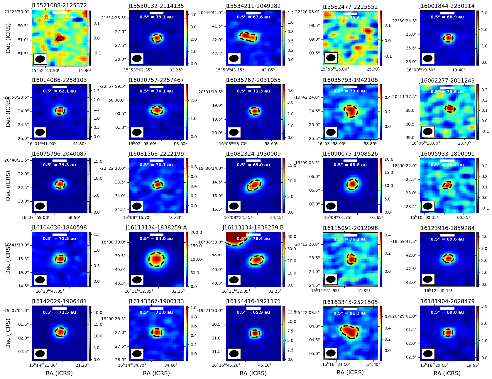
Figure 1: 345 GHz continuum images for all 25 targets in the sample. All panels are in ICRS coordinates, with a field of view of 2$\arcsec$. All colorbars are in units of mJy beam^-1. The 0.5$\times$I_peak contour for each source is shown as a black dashed line. The continuum beam for each field is shown in the bottom left corner of each image, and an angular and physical scalebar in the top center. Source J15562477-2225552 is a non-detection at 3$\sigma$.

We conducted follow-up observations in ALMA Cycle 7 of the CO-detected Barenfeld et al. (2016) targets with spectral type K5 or later. We also observe an additional target (16113134$-$1838259 B) that is in the same field as one of the Barenfeld et al. (2016) targets but not reported in that work.

The basic properties of each source are listed in Table 1. The source distances and uncertainties are derived from Gaia parallax measurements. The spectral types and T_eff come from Barenfeld et al. (2016), and references therein. Barenfeld et al. (2016) use the spectral types of Luhman & Mamajek (2012), and adopt an uncertainty of $\pm$1 spectral subclass. Barenfeld et al. (2016) then convert spectral type into T_eff using the temperature scales of Schmidt-Kaler (1982), Straižys (1992), and Luhman (1999). The T_eff uncertainties reflect the $\pm$1 spectral-subclass uncertainty.

The L_⋆ values are derived by fitting optical-infrared (OIR) photometry to BT Settl stellar atmospheric models (Allard et al., 2011) for all sources except J16113134-1838259 A & B. Sources J16113134-1838259 A & B are not separable in most OIR images, and so could not be fit with this method; for these sources, luminosities come from Eisner et al. (2005), who use OIR spectroscopy and SED modeling to derive L_⋆. Full details of our BT Settl fitting procedure, as well as plots showing OIR photometry and the best-fit BT Settl models, can be found in Appendix A.

Since the acquisition of the ALMA data, group membership information for some of the sources has been revised. One of our original targets, J16113134-1838259 A, is now explicitly identified in as belonging to $\rho$ Ophiuchus and not Upper Sco (Luhman, 2022a; Carpenter et al., 2025). However, sources J16113134-1838259 A & B are in the same field of view. For this reason, source J16113134-1838259 A is included in the tables and figures detailing our line and continuum detections (see § 2.3 below), but is excluded from our subsequent analysis. This gives us a final sample size of 24 disks.

2.3 Observing Details and Data Products

Our tuning covers ¹²CO J$=$3$-$2 (345.7959899 GHz), ¹³CO J$=$3$-$2 (330.5879653 GHz), and 870 $\mu$m (345 GHz) continuum emission (ALMA Project 2019.1.00493.S, PI P. Sheehan). The ¹²CO J$=$3$-$2 line spectral window was centered on 345.795990 GHz with 468.75 MHz bandwidth (406.4 km s^-1) and 282 kHz (0.245 km s^-1) spectral resolution. The ¹³CO J$=$3$-$2 line spectral window was centered on 330.587965 GHz with 468.75 MHz bandwidth (406.4 km s^-1) and 282.227 kHz (0.256 km s^-1) spectral resolution. The continuum data were observed in two spectral windows centered on 332 and 344 GHz, respectively, each with 1.875 GHz bandwidth and 31.25 MHz spectral resolution. We requested a target angular resolution of 0$\farcs$27 and Largest Angular Scale (LAS) of 2$\farcs$4. Our integration time was 24 minutes per target, designed to achieve 5 mJy beam^-1 sensitivity per $\sim$0.5 km s^-1 channel (assuming $\sim$2$\times$ channel binning) and 55 $\mu$Jy beam^-1 in continuum.

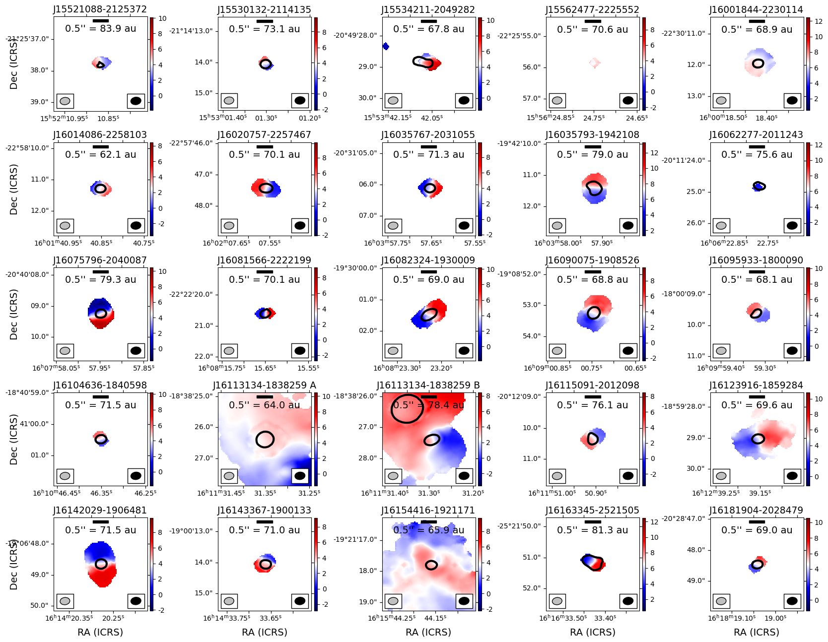
Figure 2: ¹²CO intensity-weighted velocity (moment 1) maps for all 25 targets. All panels are in ICRS coordinates, with a 4$\arcsec$ field of view. All colorbars are in km s^-1, and are centered on a V_LSR determined from a by-eye examination of each target’s spectrum. Each image is masked such that only pixels with a) S/N $>$ 2$\sigma$ in b) at least two consecutive channels and c) at least four pixels square are included in the moment maps. The 0.5$\times$I_peak continuum contours are overlaid in black. The ¹²CO beam is shown in the bottom left corner of each panel, the continuum beam in the bottom right, and an angular and physical scalebar in the top center.

The data were taken in C-4 between 27 February 2020 and 20 May 2022. All data calibration was performed by the ALMA pipeline in CASA (CASA Team et al., 2022; McMullin et al., 2007). We use the ALMA pipeline image products for the continuum data. For the line data, we resample the line cubes to 0.4 km s^-1 velocity resolution using the cvel2 task. The purpose of the resampling is to increase per-channel signal-to-noise in the image cubes for our initial search for line detections, and to reduce fitting time in our data modeling procedure (see § 3). We image the resampled data using tclean with Briggs weighting, a robust value of 0.5, and no multiscale clean for most sources. For sources with extended emission (e.g. J16113134-1838259, J16154416-1921171), we use multiscale clean and robust values between 0.0 and 1.0.

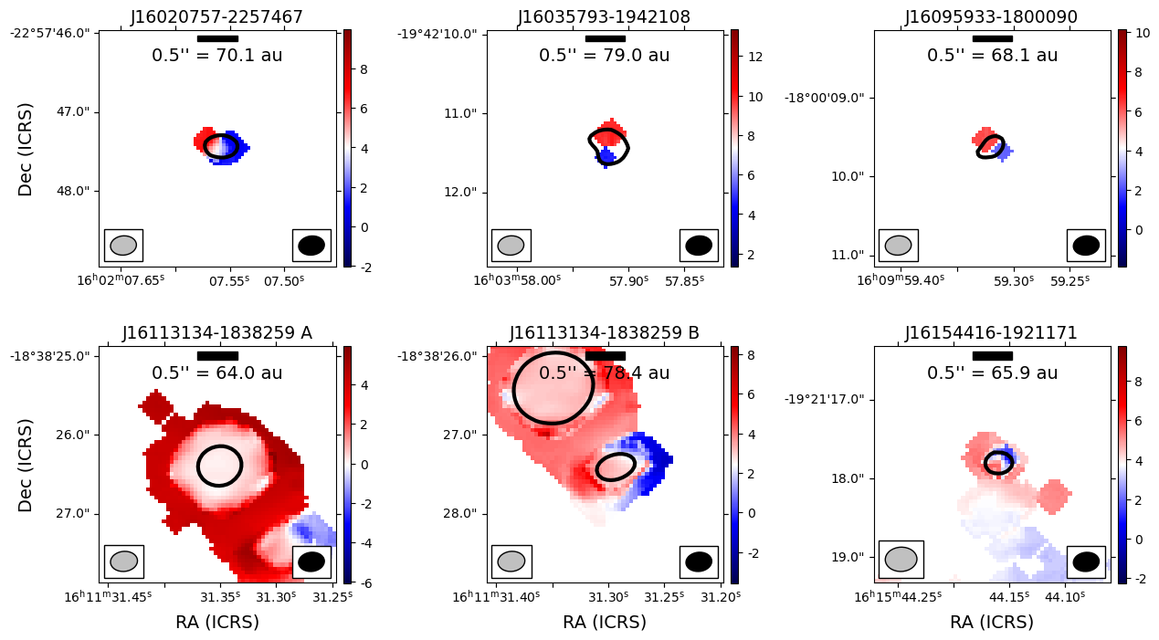
Figure 3: As in Figure 2, but for ¹³CO emission. Only sources with ¹³CO detections are shown.

For the CO line cubes, we define “detection” to mean emission $>$5$\sigma_{i}$ in at least two consecutive channels, where $\sigma_{i}$ is the rms in channel $i$. We detect ¹²CO emission associated with all 25 targets, and ¹³CO emission associated with 6/25 targets. We detect continuum emission associated with 24 out of 25 targets with a detection limit of 3$\sigma$ ($\sim$0.30-0.50 mJy beam^-1 in most cases). We use a lower detection threshold in continuum because the positions of all sources are already known from the ¹²CO detections; the statistical likelihood of multiple $>$3$\sigma$ detections at the same location in different images is much smaller than the likelihood of a 3$\sigma$ signal in a single image. The source that remains undetected in continuum is J15562477-2225552. This source has I_peak $=$ 0.113 mJy beam^-1 (1.9$\sigma$).

Table 2: Line Cube and Continuum Image Properties

Field	$\sigma_{{}^{12}CO}^{a}$	I${}^{a}_{peak,\,^{12}CO}$	12CO Moment 0 Gaussian Fitb			$\sigma_{{}^{13}CO}^{a}$	I${}^{a}_{peak,\,^{13}CO}$	$\sigma^{c}_{cont}$	I${}^{c}_{peak,\,cont}$	Continuum Gaussian Fitd
			Major	Minor	P.A.					Major	Minor	P.A.
J15521088-2125372	5.4	42.8$\pm$5.6	0.3 (0.9)	0.1 (0.06)	80 (20)	6.7	$<$33.9	0.06	0.19$\pm$0.06	1.3 (0.9)	0.1 (0.2)	110 (20)
J15530132-2114135	5.4	42.8$\pm$5.5	0.7 (0.6)	0.1 (0.3)	40 (30)	6.6	$<$31.4	0.06	4.34$\pm$0.06	0.14 (0.02)	0.11 (0.02)	50 (30)
J15534211-2049282	5.5	52.5$\pm$5.6	0.6 (0.3)	0.1 (0.1)	70 (30)	6.8	$<$33.4	0.06	1.31$\pm$0.06	0.57 (0.05)†	0.25 (0.05)†	50 (20)†
J15562477-2225552	5.5	30.5$\pm$5.3	$\cdots$	$\cdots$	$\cdots$	6.6	$<$33.2	0.06	$<$0.18	$\cdots$	$\cdots$	$\cdots$
J16001844-2230114	5.5	185.9$\pm$5.4	0.41 (0.08)	0.36 (0.07)	110 (80)	7.4	$<$31.3	0.07	3.16$\pm$0.07	0.11 (0.06)	0.08 (0.05)	30 (90)
J16014086-2258103	5.5	75.7$\pm$5.5	0.1 (0.2)	0.06 (0.07)	100 (30)	6.9	$<$33.3	0.06	2.84$\pm$0.06	0.14 (0.03)	0.09 (0.03)	80 (30)
J16020757-2257467	5.5	75.7$\pm$5.4	0.4 (0.2)	0.3 (0.3)	200 (100)	7.0	57.9$\pm$6.6	0.07	2.88$\pm$0.07	0.26 (0.02)	0.15 (0.01)	81 (6)
J16035767-2031055	5.5	67.8$\pm$5.4	0.4 (0.3)	0.2 (0.1)	110 (50)	6.8	$<$32.7	0.07	4.51$\pm$0.07	0.12 (0.01)	0.08 (0.03)	30 (20)
J16035793-1942108	5.5	111.7$\pm$5.3	0.5 (0.2)	0.3 (0.3)	170 (90)	7.0	37.4$\pm$6.3	0.07	0.58$\pm$0.07	0.41 (0.09)	0.3 (0.1)	40 (30)
J16062277-2011243	5.5	29.7$\pm$5.7	$\cdots$	$\cdots$	$\cdots$	6.7	$<$32.6	0.07	0.35$\pm$0.07	$\cdots$	$\cdots$	$\cdots$
J16075796-2040087	5.5	153.3$\pm$5.6	0.3 (0.1)	0.2 (0.2)	20 (60)	7.2	$<$33.5	0.08	15.85$\pm$0.08	0.78 (0.05)†	0.64 (0.05)†	90 (20)†
J16081566-2222199	5.5	41.2$\pm$5.3	0.4 (0.3)	0.2 (0.2)	70 (50)	6.6	$<$33.0	0.06	0.98$\pm$0.06	$\cdots$	$\cdots$	$\cdots$
J16082324-1930009	5.5	93.0$\pm$5.6	0.6 (0.3)	0.2 (0.2)	150 (30)	7.0	$<$32.8	0.09	17.25$\pm$0.09	1.05 (0.05)†	0.70 (0.05)†	140 (20)†
J16090075-1908526	5.5	86.8$\pm$5.4	0.6 (0.2)	0.4 (0.1)	160 (30)	6.8	$<$34.0	0.10	20.3$\pm$0.1	0.90 (0.05)†	0.80 (0.05)†	140 (20)†
J16095933-1800090	5.5	59.8$\pm$5.6	0.3 (0.3)	0.2 (0.1)	70 (80)	7.3	35.8$\pm$7.0	0.07	0.38$\pm$0.07	$\cdots$	$\cdots$	$\cdots$
J16104636-1840598	5.6	46.4$\pm$5.5	$\cdots$	$\cdots$	$\cdots$	6.6	$<$32.5	0.06	1.59$\pm$0.06	0.15 (0.04)	0.14 (0.06)	10 (70)
J16113134-1838259 A	6.9	809.6$\pm$7.1	1.20 (0.09)	0.91 (0.07)	60 (10)	7.9	221.4$\pm$8.2	0.87	201.2$\pm$0.9	0.462 (0.007)	0.433 (0.007)	120 (10)
J16113134-1838259 B	6.9	421.2$\pm$6.5	1.06 (0.06)	0.80 (0.04)	107 (9)	7.9	96.1$\pm$8.1	0.87	43.6$\pm$0.9	0.38 (0.01)	0.20 (0.01)	114 (3)
J16115091-2012098	5.5	65.6$\pm$5.5	0.4 (0.2)	0.3 (0.1)	100 (50)	6.6	$<$32.4	0.06	0.43$\pm$0.06	$\cdots$	$\cdots$	$\cdots$
J16123916-1859284	5.5	82.9$\pm$5.4	1.1 (0.3)	0.6 (0.1)	110 (20)	6.9	$<$32.7	0.07	4.38$\pm$0.07	0.26 (0.01)	0.183 (0.008)	99 (6)
J16142029-1906481	5.6	158.5$\pm$5.6	0.6 (0.1)	0.3 (0.1)	10 (20)	7.1	$<$34.1	0.12	22.90$\pm$0.12	0.83 (0.05)†	0.76 (0.05)†	90 (20)†
J16143367-1900133	5.6	68.4$\pm$5.5	0.3 (0.1)	0.2 (0.1)	100 (90)	7.7	$<$33.5	0.07	1.04$\pm$0.07	0.19 (0.05)	0.04 (0.09)	50 (20)
J16154416-1921171	9.4	277.0$\pm$13.3	1.28 (0.08)	0.79 (0.06)	42 (6)	11.7	78.5$\pm$12.1	0.13	14.1$\pm$0.1	0.14 (0.02)	0.12 (0.02)	50 (40)
J16163345-2521505	5.6	37.5$\pm$5.7	0.5 (0.3)	0.3 (0.2)	70 (60)	6.9	$<$34.2	0.06	0.79$\pm$0.06	0.50 (0.06)	0.27 (0.05)	70 (10)
J16181904-2028479	5.6	44.7$\pm$5.7	0.3 (0.2)	0.2 (0.2)	200 (200)	7.0	$<$34.3	0.06	3.02$\pm$0.06	0.13 (0.03)	0.09 (0.04)	120 (50)

Continuum images for all sources are shown in Figure 1. Half-peak contours (0.5$\times$I_peak,cont) are shown in black in all panels. Figure 2 shows ¹²CO intensity-weighted velocity (moment 1) maps for all 25 sources, with the 0.5$\times$I_peak,cont continuum contours overlaid. Figure 3 shows ¹³CO moment 1 maps for sources with I${}_{peak,^{13}CO}$ $>$ 5$\sigma$, again with the 0.5$\times$I_peak,cont continuum contours overlaid. Continuum and median line noise (rms) values are listed in Table 2, along with peak intensities and upper limits. Beam sizes are nearly identical for all sources: (0$\farcs$31-0$\farcs$32)$\times$0$\farcs$23 for the ¹²CO cubes, (0$\farcs$34-0$\farcs$35)$\times$0$\farcs$26 for the ¹³CO cubes, and 0$\farcs$33$\times$0$\farcs$24 for the continuum images. The beam size consistency is a result of our observing strategy; all fields were observed in all scheduling blocks.

2.4 Disks vs Bipolar Outflows

Given the relationship between accretion and ejection (e.g. Frank et al., 2014), it is reasonable to consider whether the CO emission in these sources is tracing disk winds/outflows in addition to (or instead of) a rotating disk. The canonical morphological indicator of an outflow is a $\sim$90^∘ misalignment between the observed disk major axes in continuum and line emission. We examine our data for such a signature. We use the imfit task in CASA to fit 2-dimensional Gaussians to the ¹²CO moment 0 maps, and to the 870 $\mu$m continuum data. We list the deconvolved imfit sizes of all sources in Table 2. Six sources appear to be reasonably well-resolved in the continuum: J15534211$-$2049282, J16035793$-$1942108, J16082324$-$1930009, J16090075$-$1908526, J16113134$-$ 1838259 B, and J16163345$-$2521505. We compare the continuum and ¹²CO moment 0 position angles for these six sources. In Figure 4, we show close-in views of the moment 0 and moment 1 maps for these sources, with 870 $\mu$m continuum contours overlaid.

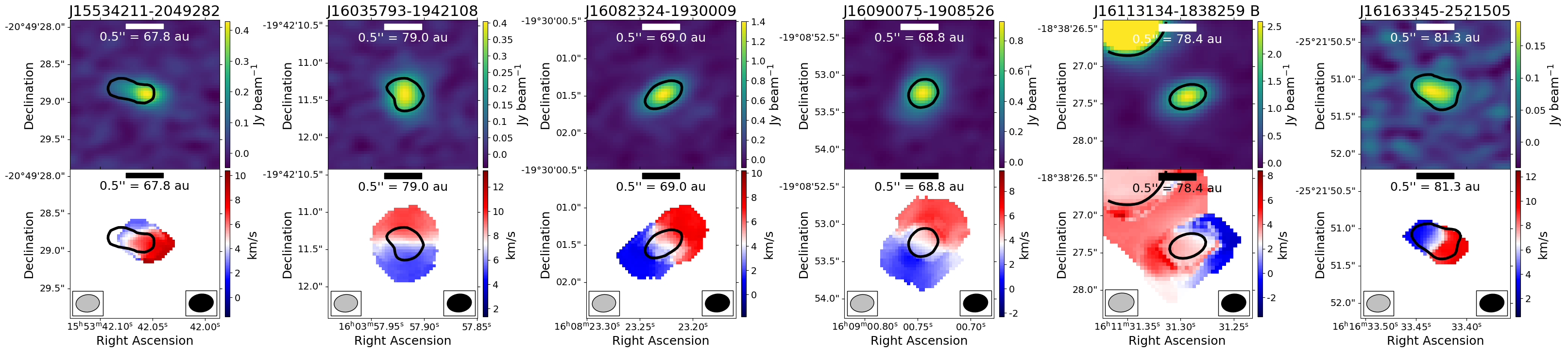
Figure 4: Moment 0 (top row) and moment 1 (bottom row) maps of the six sources whose continuum emission is reasonably well-resolved. The moment maps show ¹²CO emission in all cases except J16113134-1838259 B, which show ¹³CO. 870 $\mu$m continuum contours are overlaid in black; the contours show the 0.5$\times$I_peak level. The ¹²CO beams are shown in the bottom left corner of the moment 1 images, and the continuum beams are shown in the bottom right corner.

The position angles of the continuum and moment-0 line emission agree within uncertainties for all six sources. Furthermore, as seen in Figure 4, the position angles of the continuum disks’ major axes correspond to the direction of the velocity gradients seen in the moment 1 maps. This is consistent with Keplerian rotation. These findings together are consistent with the interpretation that the CO is tracing disk gas and not outflows. While we cannot rule out dust-gas disk misalignment for the remaining 18 sources, we find no evidence for this in our sample, and good evidence in favor of the assumption that the CO is tracing disk gas.

3 Disk Model Fitting

The Keplerian rotation of a protoplanetary disk is a direct probe of the enclosed mass. However, because deriving source mass from Keplerian velocity requires knowing linear distances $r$ within the disk, and $r$ = $\theta$ $\times$ distance (where $\theta$ is the angular size), deriving high-accuracy stellar masses requires high-precision source distances. Gaia has produced extremely high-precision parallactic distance measurements for many nearby pre-main sequence stars, including all of our targets in Upper Sco.

We use our high-sensitivity ALMA CO data, combined with the Gaia distances, to fit a Keplerian disk model to each of our targets and derive enclosed stellar mass. We use the open-source, python-based pdspy package to perform Markov Chain Monte Carlo (MCMC) fitting of disk models to our data in visibility space ($u,v$). We use radmc3d (Dullemond et al., 2012) to generate the disk models, galario (Tazzari et al., 2018) to transform the model data from image space to Fourier space, and the emcee package (Foreman-Mackey et al., 2013) for the MCMC fitting. We describe our fitting procedure and convergence criteria in greater detail in the following sections.

3.1 The Model

In pure Keplerian rotation, the azimuthal velocity at any given stellocentric radius $r$ is given by

$$v_{\phi}(r)=\sqrt{\frac{G\,M_{encl}}{r}},$$ (1)

where $G$ is the gravitational constant and M_encl is the total mass enclosed within the radius $r$. The corresponding observed velocity is

$$v_{obs}(r)=v_{\phi}(r)sin(i)$$ (2)

where $i$ is the inclination angle of the disk ($i$ = 0 being face-on, and $i$=90 being edge-on).

In reality, the fluid dynamics and, especially, the pressure gradients in disks can result in sub-Keplerian velocities (e.g. Haworth et al., 2018; Sanna et al., 2019). Therefore, these effects must be accounted for as well. We use an exponentially-tapered flared disk model based on the viscous-disk models of Lynden-Bell & Pringle (1974). The model has an azimuthally-symmetric radial structure with surface density given by

$$\Sigma(r)=\Sigma_{0}\left(\frac{r}{r_{c}}\right)^{-\gamma}exp\left[-\left(\frac{r}{r_{c}}\right)^{2-\gamma}\right].$$ (3)

Here, $r_{c}$ is the radius beyond which the disk is exponentially tapered, $\gamma$ is the surface density power-law exponent, and $\Sigma_{0}$ is given by

$$\Sigma_{0}=\frac{(2-\gamma)M_{d}}{2\pi r_{c}^{2}},$$ (4)

where $M_{d}$ is the total disk gas mass. The disk flaring and scale-height parameters are calculated assuming hydrostatic equilibrium. The disk scale height is given by

$$h(r)=\left[\frac{k_{b}\,r^{3}\,T_{gas}(r)}{G\,M_{\star}\,\mu\,m_{H}}\right],$$ (5)

where $M_{\star}$ is the stellar mass and $\mu$ = 2.37 is the mean molecular weight of the gas assuming solar metallicity. The model assumes the disk is vertically isothermal, with a radial temperature dependence given by

$$T_{gas}(r)=T_{0}\left(\frac{r}{1\,\,au}\right)^{-q},$$ (6)

where $T_{0}$ is the temperature at 1 au and $q$ is the temperature power-law exponent.

These assumptions together give a 2-dimensional density structure of

$$\rho(r,z)=\frac{\Sigma(r)}{\sqrt{2\pi}\,h(r)}exp\left[-\frac{1}{2}\left(\frac{z}{h(r)}\right)^{2}\right],$$ (7)

where $z$ is the height above the disk midplane. Further details of this model and its implementation in pdspy can be found in Sheehan et al. (2019).

Following the method of Sheehan et al. (2019), we use 15 free parameters: the offset from the source sky center position (RA_off, Dec_off), distance ($d$), disk position angle (P.A.), inclination angle ($i$), and source velocity (V_LSR); stellar mass (M_⋆), disk mass (M_d), disk inner radius (R_in) and outer radius (R_d); disk temperature at 1 au ($T_{0}$), disk temperature power-law exponent ($q$), stellar luminosity (L_⋆), disk surface density power-law exponent ($\gamma$), and disk turbulence ($a_{turb}$). (We note that, in practice, L_⋆ has very little impact on the fit results, as it is not directly incorporated into the disk model.) The molecular-to-H₂ abundance ratios are fixed in all fits. We adopt a CO/H₂ abundance of 10^-4 (Allen, 1973; Encrenaz et al., 1975; Dickman, 1978). We adopt a ¹³CO/H₂ abundance ratio of 10^-5.3, based on the assumption of a ¹²CO/¹³CO ratio of 20:1 from literature observations of protoplanetary disks (Bergin et al., 2024; Semenov et al., 2024).

3.2 Allowed Ranges for Free Parameters

The free parameters and their allowed ranges are listed in Table 3. For ease of computation over multiple orders of magnitude, pdspy calculates stellar mass, disk mass, disk inner and outer radius, disk inner edge temperature, turbulence, and luminosity in log space. Distance, L_⋆, V_LSR, and position have ranges and initial values unique to each target. The allowed ranges for most other free parameters were the same for all sources (see Table 3), with the exception of position angle (P.A.) and temperature power-law slope ($q$). The conditions under which adjustments to these parameters were necessary are described in § 3.3.

3.2.1 $D$ and L_⋆

For a Gaussian distribution, $\pm$2$\sigma$ will encompass $\pm$95% of the distribution of the measured values. We restrict $D$ to each target’s Gaia-measured distance plus or minus twice its upper and lower limits, where the distance limits are calculated from the Gaia upper and lower limits on parallax. We restrict L_⋆ to the value reported in Table 1 for each source, plus or minus twice its associated uncertainty.

3.2.2 V_LSR, RA_off, and Dec_off

Our position and velocity initial values are estimated from the image cubes, and their allowed ranges reflect our uncertainty in this initial estimation. By default, we allow velocity to vary over V_LSR$\pm$1.2 km s^-1 (corresponding to $\pm$3 channels), where the V_LSR is determined from a by-eye examination of the ¹²CO image cube and integrated spectrum. For some sources, especially those with low signal-to-noise ratios, our ability to estimate V_LSR by eye is more limited, and we expand the parameter range to V_LSR$\pm$2.4 km s^-1 ($\pm$6 channels). We estimate the center position of each disk by fitting a 2D gaussian in the image plane using the imfit task in CASA. We calculate the distance from image center to disk center in RA and Dec, and use these as our initial values for RA_off and Dec_off. We restrict the parameter range to this initial guess $\pm$0.25 arcsec, or about $\pm$6 pixels ($\sim$0$\farcs$04 each). This range is $\sim$2-3$\times$ the typical uncertainty on the imfit results.

Table 3: pdspy Parameter Ranges

Parametera	Units	Default Range
Distance ($D$)	pc	$D_{Gaia}-2(\sigma_{low}$/$\sigma_{upp}$)
Velocity (VLSR)	km s-1	vcen $\pm$ 1.2
RA offset (RAoff)	″	RA $\pm$ 0.25
Dec offset (Decoff)	″	Dec $\pm$ 0.25
Inclination ($i$)	∘	[0, 180]
Position Angle (P.A.)	∘	[0, 360]
Stellar Mass (M⋆)	log(M⊙)	[$-$1.5, 1.5]
Disk Mass (Md)	log(M⊕)	[$-$10, $-$2.5]
Outer Radius (Rd)	log(AU)	[0, 4]
Inner Radius (Rin)	log(AU)	[$-$1, Rd)
Temp at 1 au (T0)	log(K)	[0, 3.5]
T(r) exponent ($q$)	$\cdots$	[0, 1]
Turbulence ($a_{turb}$)	log(km s-1)	[$-$1.5, 1]
Luminosity ($L_{\star}$)	log(L⊙)	L⋆ $\pm$ 2$\sigma_{L_{\star}}$
$\Sigma$ exponent ($\gamma$)	$\cdots$	[$-$0.5, 2)

3.2.3 M_⋆, M_disk, R_in, R_d, T₀, $\alpha_{turb}$, $i$, and $\gamma$

The allowed range for stellar mass (log(M_⋆) $=$ [-1.5,1.5], M_⋆ $=$ [0.03,30] M_⊙) encompasses all expected stellar mass values for our K- and M-type targets. The disk mass, outer radius, temperature at 1 au, and turbulence ranges are chosen to encompass reasonable expected values based on literature results for protoplanetary disks and the viscous, hydrostatic disk model. The lower limit for disk inner radius is chosen to account for the absolute minimum physical resolution we can reasonably expect to achieve with our data (0.1 au). For the disk inner radius upper limit, the model requires R_in $<$ R_d at all times. The range for $i$ allows for the possibility of differentiating between momentum vectors of equal magnitude but opposite line-of-sight directions (i.e. clockwise versus counterclockwise rotation for a source at a given $i$). The range for $\gamma$ (the surface-density power-law exponent) reflects both the disk model itself and our data. A lower limit of $\gamma$ $=$ $-$0.5, representing a sharply tapered disk surface density, is the the lower limit of what we can reasonably expect to constrain with our data.

3.3 Fitting Procedure

MCMC fitting involves using “walkers,” which are individual evaluations of the model for different values of the model parameters. The $\chi^{2}$ value of each walker is compared to that of another random walker in the set, and then the parameters of the original walker are adjusted toward or away from the comparison walker by a semi-randomized amount. One round of comparison and adjustment for all walkers is a single “step” of the MCMC fit. The walkers’ initial distribution in parameter space (the “priors”) are set by the user. A uniform prior means that walkers are distributed uniformly across the parameter range, while a Gaussian prior means that more walkers have initial values close to the center of the parameter space, etc. Full details of the MCMC procedure in general can be found in Foreman-Mackey et al. (2013), and details of its implementation in pdpsy can be found in Sheehan et al. (2019).

In this work, we use 200 walkers for all fits. We assume uniform priors for all parameters except source distance and stellar mass. For distance, we use a Gaussian distribution in parallax, where the distribution is centered on the Gaia parallax value and has a width of 2$\log$(2)$\times\sigma_{Gaia}$. We then calculate source distances from this distribution in parallax. For stellar mass, the initial distribution of walkers is set using the Charbrier IMF.

Most MCMC procedures use a “burn-in” interval, i.e. some initial number of steps which will not be considered when determining the final MCMC results. The goal is to allow the walkers time to settle from their initial distributions into - ideally - higher-probability regions for each parameter. Burn-in is most important when the MCMC best-fit values are calculated using bulk statistics (median, mean, $\sigma$) for all walkers and steps, such as the median-value method used in Sheehan et al. (2019). We use a minimum burn-in interval of 1000 steps, though some sources required longer (e.g. 4500 steps for J16075796-2040087).

After burn-in, we check the distribution of walkers for each parameter and adjust parameter ranges as needed for individual sources. If any parameter range changes, we restart the pdspy fitting for the source in question from 0 steps. The circumstances in which this was necessary are described in § 3.3.1, below. At 2500 steps, we begin evaluating the log(M_⋆) parameter for convergence. Our convergence criteria are discussed in § 3.3.2, below. If the stellar mass has converged at 2500 steps, we stop the fit. If the stellar mass has not converged, we continue the fit until the convergence criteria are met. If the walker distributions at 2500 steps indicate that further adjustments to the parameter ranges are needed, we adjust the ranges, restart the fit from 0 steps, and evaluate the new fits at 1000 and 2500 steps as previously described. For most sources, the walkers meet the convergence criteria within $\sim$6500 total steps.

3.3.1 Modifying Parameter Ranges and Restarting Fits

For most parameters, it was not necessary to make adjustments to the parameter ranges after 1000 steps. However, two parameters required adjustment for $>$25% of the sample: position angle (P.A.) and temperature exponent ($q$). In the case of position angle, all sources had a total range of 360^∘, but some sources had limits of [$-$180^∘,180^∘] or [$-$90^∘,270^∘] instead of [0^∘,360^∘]. This is for purely practical purposes: sources with position angles of $\sim$270^∘ $\leq$ $\theta$ $\leq$ 90^∘ often had some a fraction of their walkers “pile up” near the edge of the parameter range, causing a false bimodal distribution. Resetting the position-angle range resulted in single solutions for position angle in all cases.

In the case of $q$, we initially used a range of [0,1], i.e. a flat to linearly-decreasing temperature with radius, for all sources. In some cases, however, most or all walkers were clustered near the top of the $q$ $=$ [0,1] range, with solutions showing no significant improvement over at least 1000 post-burn-in steps (this is the autocorrelation time for 200 walkers and 15 degrees of freedom for our disk model; see Sheehan et al., 2019). For these sources, we expand the parameter range to $q$ $=$ [0,2], i.e., between flat and a quadratic decrease in temperature with radius.

3.3.2 Stopping Criteria

The point at which an MCMC fit has converged does not have a universally agreed-upon definition (see Roy, 2020, for a recent review). The mathematical basis of MCMC fitting says that, in theory, all walkers will converge to the same value for a given parameter, if given infinite time. This is, for obvious reasons, not a useful definition in practice. As a practical matter, most MCMC users apply empirical stopping criteria instead, such as fixed-width or relative fixed-width stopping rules, variance-based estimates, and density-based estimates (see e.g. Roy, 2020, and references therein).

For the purposes of this work, we adopt a relative variance-based stopping rule in which we define “convergence” to mean that the value of log(M_⋆) has varied by less than 1% over a given interval. Our assessment procedure is as follows: at each step past the initial burn-in (see § 3.3), we apply a $\chi^{2}$ cut to the data to remove any walkers outside the 99th percentile ($\sim$2.5$\sigma$ for a normal distribution). We require that at least 101 walkers (i.e. a majority) survive the $\chi^{2}$ cut.

Once $\geq$101 walkers remain, we make trace plots for each source in order to evaluate convergence. To construct the trace plots, we calculate the mean, standard deviation, median, and median absolute deviation (MAD) of log(M_⋆) for each step. The standard deviation and scaled MAD serve as the uncertainties for the mean and median, respectively. We calculate the slope of the mean and median versus step over the previous 1000 steps, with each data point weighted by its uncertainty. We choose the last 1000 steps for this fit because this is the autocorrelation time for an MCMC fit with 200 walkers and 15 free parameters (see e.g. Sheehan et al., 2019). If the magnitude of the slope over the last 1000 steps is less than 1% of the value of the parameter itself, we consider the slope to be converged. We require that both median and mean be converged in order to stop the fitting. Representative trace plots from source J16090075-1908526 are shown in Figure 5. Trace plots of log(M_⋆) versus step number for each source can be found in Appendix A.

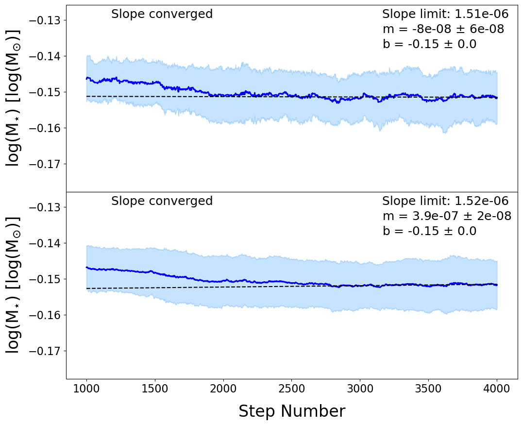
Figure 5: Representative example of the trace plots we used to determine fit convergence. The example shown is for source J16090075-1908526. In both panels, the first 1000 steps are excluded from plotting as they are considered burn-in steps. Top: The blue line is the median value of all walkers at each step. The blue shaded region is the scaled median absolute deviation from the median (scaled MAD) at each step, and is used to weight the linear fit. The black dotted line shows the best-fit line for the last 1000 steps. Properties of the best-fit line are listed in the upper right corner. Bottom: Same as for the top panel, except that the blue line is the mean value of all walkers and each step and the blue shaded region is the standard deviation at each step.

3.4 Comparing Methods of Deriving Parameter Values and Uncertainties

In addition to convergence criteria, choosing how to report the value and uncertainty for each parameter can also introduce some arbitrariness to the results. By default, pdspy reports the median of all walker positions over all post burn-in steps as the parameter value, and the standard deviation of those values as the uncertainty on that value. Sheehan et al. (2019) report the walkers’ median as the parameter value and the $\pm$95% percentile range as the parameter uncertainty.

We explore how the $\chi^{2}$ best-fit values and their associated uncertainties compare to the median and standard deviation of walker positions. This exploration was motivated by the possibility that 1$\sigma$ values calculated from $\Delta\chi^{2}$ might be larger than the walker standard deviations, which can occur when there is not a significant difference in $\chi^{2}$ between the best fit and the next-best fit. For this comparison, we use only those walkers meeting the 99% $\chi^{2}$ cut within the previous 1000 steps, in order to calculate our best-fit values over the same interval as we calculated the fit convergence.

We calculate the median and standard deviation of the parameter values using the default pdspy settings. We also determine the fit with the lowest $\chi^{2}$ value, and extract the parameter values used for that fit. We derive uncertainties for those best-$\chi^{2}$ parameters using the change in $\chi^{2}$. For a model with 15 free parameters, a value of $\Delta\chi^{2}$ $=$ 15.975 corresponds to a 1$\sigma$ uncertainty (Press et al., 1992). We calculate the lower- and upper-bound uncertainties as the minimum and maximum parameter values across all fits with $\chi^{2}$ $\leq$ $\chi^{2}_{min}$ $+$ $\Delta\chi^{2}$ within the last 1000 steps.

We find that the minimum $\chi^{2}$- and median-derived parameter values typically agree within uncertainties, but can have up to a $\sim$1$\sigma$ disagreement (where $\sigma$ is derived using $\Delta\chi^{2}$). More notably, we find that the standard deviation-based uncertainties are systematically lower than the $\Delta\chi^{2}$-based uncertainties by factors of $\sim$2-3. The median standard deviation-based uncertainty in log(M_⋆) is 9$\pm$7%, whereas the median lower- and upper-bound $\Delta\chi^{2}$ uncertainties are 17$\pm$11% and 30$\pm$25%, respectively.

Figure 6 shows a corner plot with the distribution of walker values for each parameter for source J16082324-1930009. The median and standard deviation-based parameter values and uncertainties are shown in black, and the $\Delta\chi^{2}$-based parameter values and uncertainties are shown in red. These plots and the calculations above suggest that adopting the standard deviation (or even scaled MAD) of walker positions as the parameter uncertainty could give the false impression that a parameter is more well-constrained than it is. In this work, we report the parameter values from the minimum-$\chi^{2}$ fit, and determine upper- and lower-bound uncertainties using $\Delta\chi^{2}$.

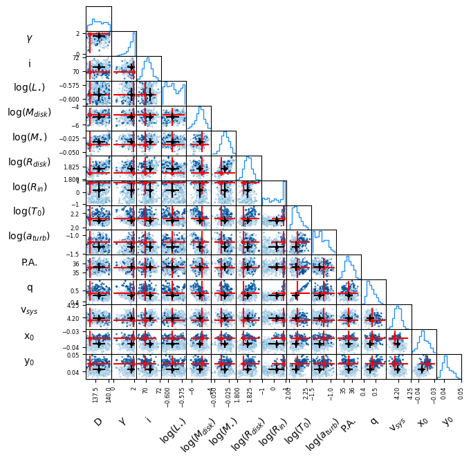
Figure 6: Corner plot showing the distribution of walker values for each parameter for the last 1000 steps. This example is for source J16082324-1930009. The “x₀” and “y₀” labels refer to the RA and Dec offsets, respectively. The data points are colored by their $\chi^{2}$ values, with darker colors indicating lower $\chi^{2}$. Median walker values are shown in black, with standard deviations shown as black error bars. The $\chi^{2}$ best-fit values are shown in red, with the $\Delta\chi^{2}$-based uncertainties shown as red error bars. The median- and $\chi^{2}$-based best-fit values typically agree within uncertainties, but can clearly disagree by up to $\sim$1 standard deviation. The potential underestimation of uncertainties from the standard deviation method as opposed to the $\Delta\chi^{2}$ method can be clearly seen.

4 Results

We successfully fit the CO data for 23 out of 24 sources: ¹²CO J$=$3$-$2 for 22 of our 24 sources, and ¹³CO J$=$3$-$2 for 4 out of the 5 sources with ¹³CO detections. We also obtained joint ¹²CO$+^{13}$CO fits for the three sources that had usable data in both lines. We were unable to fit the ¹²CO data for J16113134-1838259 B and any of the line data for J16154416-1921171. We discuss these sources, as well as sources which required special handling during the fitting process or returned results significantly at odds with the literature, in greater detail in Appendix B.

In general, parameters related to the geometry and kinematics of the source ($i$, $\theta$, RA_off, Dec_off, V_LSR, M_⋆) are well-constrained by our fitting procedure. We note that inclination angle ($i$) has a bimodal solution for nearly all sources, with the two solution values approximately equidistant from $i$ $=$ 90^∘. This indicates that we are not differentiating between clockwise and counterclockwise rotation for any targets.

We show M_⋆, V_LSR, $i$, position angle, and center coordinate offsets for each ¹²CO fit in Table 4. We show M_⋆ and $i$ for the ¹³CO-only and ¹²CO$+^{13}$CO fits in Table 5. Machine-readable and ASCII tables showing the results for all free parameters for each source and line combination are available in the online material. For the three sources with usable emission in both CO isotopologues, we find that our results for the ¹²CO, ¹³CO, and ¹²CO$+^{13}$CO fits all agree within uncertainties. However, the uncertainties on the ¹³CO-only fit results are a factor of 2-14$\times$ larger than the others. This is likely due to the lower signal-to-noise ratios in our ¹³CO detections as compared to ¹²CO (see Table 2). The ¹²CO$+^{13}$CO fits typically have uncertainties that are lower than or comparable to the ¹²CO-only fits.

Table 4: ¹²CO Fit Results

Fielda	N${}_{steps}^{b}$	M${}_{\star}^{c}$	VLSR	$i$	P.A.	RA${}_{off}^{d}$	Dec${}_{off}^{d}$
		(M⊙)	(km s-1)	(∘)	(∘)	(mas)	(mas)
J15521088-2125372	4009	0.16${}^{+0.04}_{-0.03}$	4.1${}^{+0.2}_{-0.1}$	110.0${}^{+10.0}_{-20.0}$	181.0${}^{+7.0}_{-7.0}$	-40${}^{+10}_{-10}$	4${}^{+8}_{-9}$
J15530132-2114135	7343	0.25${}^{+1.0}_{-0.09}$	3.9${}^{+0.2}_{-0.2}$	140.0${}^{+30.0}_{-30.0}$	138.0${}^{+9.0}_{-20.0}$	-80${}^{+10}_{-20}$	-50${}^{+10}_{-10}$
J15534211-2049282	15634	0.6${}^{+0.6}_{-0.1}$	4.4${}^{+0.6}_{-2.0}$	108.0${}^{+5.0}_{-7.0}$	-22.0${}^{+7.0}_{-4.0}$	-120${}^{+60}_{-10}$	-10${}^{+10}_{-20}$
J15562477-2225552	3780	$\leq$1.9	3.6${}^{+0.2}_{-0.2}$	160.0${}^{+20.0}_{-20.0}$	250.0${}^{+20.0}_{-90.0}$	-7${}^{+30}_{-10}$	20${}^{+20}_{-10}$
J16001844-2230114	18539	0.5${}^{+3.0}_{-0.3}$	6.49${}^{+0.02}_{-0.03}$	9.0${}^{+9.0}_{-5.0}$	217.0${}^{+5.0}_{-3.0}$	-37${}^{+4}_{-3}$	14${}^{+4}_{-2}$
J16014086-2258103	8015	0.25${}^{+0.25}_{-0.05}$	2.45${}^{+0.07}_{-0.08}$	135.0${}^{+20.0}_{-8.0}$	-13.0${}^{+5.0}_{-7.0}$	-47${}^{+4}_{-7}$	18${}^{+5}_{-5}$
J16020757-2257467	3502	0.53${}^{+0.05}_{-0.04}$	3.96${}^{+0.06}_{-0.05}$	61.0${}^{+3.0}_{-4.0}$	168.0${}^{+2.0}_{-2.0}$	-6${}^{+6}_{-5}$	-1${}^{+7}_{-5}$
J16035767-2031055	9209	4.0${}^{+4.0}_{-2.0}$	3.9${}^{+0.08}_{-0.06}$	17.0${}^{+10.0}_{-5.0}$	-16.0${}^{+3.0}_{-4.0}$	-60${}^{+7}_{-5}$	-30${}^{+6}_{-6}$
J16035793-1942108	7369	0.56${}^{+0.05}_{-0.04}$	7.33${}^{+0.03}_{-0.02}$	50.0${}^{+3.0}_{-2.0}$	92.0${}^{+2.0}_{-2.0}$	-98${}^{+4}_{-5}$	33${}^{+4}_{-4}$
J16062277-2011243	5505	0.3${}^{+0.3}_{-0.1}$	6.3${}^{+0.2}_{-0.2}$	60.0${}^{+30.0}_{-30.0}$	10.0${}^{+10.0}_{-20.0}$	-150${}^{+30}_{-20}$	-20${}^{+20}_{-20}$
J16075796-2040087	6214	1.9${}^{+0.2}_{-0.2}$	4.46${}^{+0.03}_{-0.05}$	52.0${}^{+1.0}_{-3.0}$	280.0${}^{+1.0}_{-1.0}$	-97${}^{+2}_{-2}$	15${}^{+1}_{-3}$
J16081566-2222199	6011	0.5${}^{+0.1}_{-0.08}$	3.3${}^{+0.2}_{-0.2}$	120.0${}^{+10.0}_{-10.0}$	3.0${}^{+6.0}_{-5.0}$	-3${}^{+10}_{-20}$	20${}^{+10}_{-10}$
J16082324-1930009	6024	0.91${}^{+0.04}_{-0.02}$	4.19${}^{+0.05}_{-0.03}$	110.0${}^{+1.0}_{-2.0}$	36.0${}^{+1.0}_{-1.0}$	-34${}^{+5}_{-5}$	44${}^{+5}_{-4}$
J16090075-1908526	4004	0.71${}^{+0.03}_{-0.03}$	3.69${}^{+0.02}_{-0.02}$	125.0${}^{+2.0}_{-2.0}$	65.3${}^{+1.0}_{-0.9}$	-43${}^{+5}_{-5}$	2${}^{+5}_{-4}$
J16095933-1800090	2817	0.25${}^{+0.05}_{-0.02}$	4.11${}^{+0.04}_{-0.06}$	126.0${}^{+9.0}_{-6.0}$	148.0${}^{+2.0}_{-5.0}$	-70${}^{+10}_{-10}$	22${}^{+15}_{-6}$
J16104636-1840598	5008	0.13${}^{+0.07}_{-0.05}$	4.2${}^{+0.1}_{-0.1}$	80.0${}^{+30.0}_{-30.0}$	124.0${}^{+8.0}_{-10.0}$	-58${}^{+19}_{-8}$	0${}^{+10}_{-10}$
J16115091-2012098	2500	0.31${}^{+0.05}_{-0.03}$	2.48${}^{+0.07}_{-0.04}$	127.0${}^{+6.0}_{-8.0}$	211.0${}^{+3.0}_{-3.0}$	-23${}^{+10}_{-6}$	16${}^{+9}_{-9}$
J16123916-1859284	3133	0.76${}^{+0.11}_{-0.07}$	4.79${}^{+0.04}_{-0.02}$	51.0${}^{+4.0}_{-5.0}$	16.0${}^{+1.0}_{-1.0}$	-21${}^{+9}_{-6}$	-32${}^{+12}_{-5}$
J16142029-1906481	10158	1.32${}^{+0.06}_{-0.06}$	3.88${}^{+0.02}_{-0.02}$	60.2${}^{+0.8}_{-0.6}$	277.3${}^{+0.5}_{-0.7}$	-37${}^{+3}_{-2}$	8${}^{+2}_{-2}$
J16143367-1900133	2504	0.23${}^{+0.05}_{-0.04}$	3.15${}^{+0.07}_{-0.07}$	104.0${}^{+3.0}_{-2.0}$	227.0${}^{+5.0}_{-6.0}$	-65${}^{+7}_{-6}$	11${}^{+4}_{-7}$
J16163345-2521505	2500	0.8${}^{+0.1}_{-0.1}$	6.5${}^{+0.1}_{-0.2}$	119.0${}^{+6.0}_{-9.0}$	-27.0${}^{+5.0}_{-3.0}$	-70${}^{+20}_{-10}$	-10${}^{+10}_{-20}$
J16181904-2028479	5214	0.25${}^{+0.15}_{-0.05}$	4.6${}^{+0.1}_{-0.1}$	130.0${}^{+10.0}_{-20.0}$	50.0${}^{+10.0}_{-6.0}$	-10${}^{+10}_{-10}$	0${}^{+10}_{-10}$

Because radiative-transfer MCMC fitting is a time- and computing resource-intensive procedure, the tradeoff between the time to complete an individual step and the total number of steps required to achieve convergence may be of interest to some readers. We find that the ¹²CO$+^{13}$CO fits tend to converge in fewer steps than the single-line fits. This is not a universal result, however. In the case of J16095933-1800090, the joint fit took slightly longer to converge than the ¹²CO fit (3013 steps versus 2817 steps). J16095933-1800090 is the faintest ¹³CO detection in the sample at just 5.1$\sigma$, and this low signal-to-noise may have contributed to the increase in convergence time. Our results for these three sources suggest that jointly fitting multiple lines can be an overall time-saving approach, but only if all lines are sufficiently strong (S/N $\gtrsim$ 6$\sigma$).

Table 5: ¹³CO and Joint ¹²CO$+$¹³CO Fit Results

	12CO			13CO			12CO$+$13CO
	Steps	M⋆	i	Steps	M⋆	i	Steps	M⋆	i
Fielda		(M⊙)	(∘)		(M⊙)	(∘)		(M⊙)	(∘)
J16020757-2257467	3502	0.54${}^{+0.05}_{-0.04}$	61${}^{+3}_{-4}$	4003	0.52${}^{+0.17}_{-0.09}$	60${}^{10}_{-13}$	2949	0.52${}^{+0.03}_{-0.03}$	60${}^{+3}_{-3}$
J16035793-1942108	7369	0.56${}^{+0.05}_{-0.03}$	50${}^{+3}_{-2}$	6003	0.77${}^{+0.68}_{-0.32}$	40${}^{+19}_{-11}$	2520	0.56${}^{+0.04}_{-0.04}$	50${}^{+2}_{-3}$
J16095933-1800090	2817	0.23${}^{+0.05}_{-0.02}$	126${}^{+9}_{-6}$	3896	0.22${}^{+0.19}_{-0.05}$	130${}^{+19}_{-18}$	3013	0.25${}^{+0.03}_{-0.03}$	129${}^{+7}_{-7}$
J16113134-1838259 B	$\cdots$	$\cdots$	$\cdots$	2520	1.5${}^{+0.1}_{-0.1}$	65${}^{+1}_{-4}$	$\cdots$	$\cdots$	$\cdots$

Across the full sample and using the highest-confidence best-fit parameters for each source, we find minimum and maximum stellar masses of 0.13${}^{+0.05}_{-0.07}$ M_⊙ (for J16104636-1840598) and 4.0${}^{+2.0}_{-4.0}$ M_⊙ (for J16035767-2031055). The sample median and mean masses are M_⋆ = 0.51$\pm$0.26 M_⊙ and M_⋆ = 0.76$\pm$0.84 M_⊙, respectively, where the uncertainties are the sample standard deviation and scaled MAD. The median lower-bound uncertainty is 0.06 M_⊙ (or, 16% of the mass of a given source), and the median upper-bound uncertainty is 0.09 M_⊙ (or, 19% of the source mass).

5 Analysis

The following analysis excludes source J16154416-1921171, which could not be fit (see § 4). This gives us a total of 23 sources with dynamically-constrained masses .

The reliability and accuracy of pre-main sequence evolutionary tracks for deriving PMS masses and ages is a matter of great concern to the star- and planet-formation communities. Keplerian masses are an independent measurement of stellar mass, and can serve as a powerful evaluation tool for isochronal models. For example, Barenfeld et al. (2016) use the PMS evolutionary models of Siess et al. (2000) to derive M_⋆ for their sample. We find that our median and mean dynamical masses are 70% and 105% larger, respectively, than the isochronal masses derived by Barenfeld et al. (2016) for these same sources. Our minimum dynamical mass is consistent with that of Barenfeld et al. (2016), but our maximum dynamical mass is $\sim$4$\times$ larger. The higher-mass outlier sources are almost certainly the reason for our higher mean mass, but cannot fully explain our higher median mass. Potential explanations for these trends are discussed in detail in § 5.2 and Appendix D.1, respectively. We find median lower- and upper-bound mass uncertainties of 16% and 19%, respectively, as discussed above. This is a moderate improvement over the results of Barenfeld et al. (2016), which have median lower- and upper-bound uncertainties of 24% and 26%, respectively, for masses derived using T_eff, L_⋆, and the isochrones of Siess et al. (2000).

5.1 Stellar Evolutionary Models Considered

To more robustly compare our dynamical results with isochronal methods, we re-derive isochronal masses and ages for each source using the L_⋆ and T_eff in Table 1 and five sets of evolutionary models: the BHAC15 tracks of Baraffe et al. (2015), the PARSEC v1.1 and 1.2S tracks of Bressan et al. (2012) and Chen et al. (2014), respectively, and both the non-magnetic and magnetic tracks of Feiden (2016). We briefly describe each set of tracks in Appendix E. Figure 7 shows T_eff and L_⋆ values for our targets overlaid on isochrone contours for each set of models. We compare our dynamical results to the isochrone-derived results for each model set and evaluate which, if any, agree consistently with the dynamical results. In this paper, we focus on the dynamical masses as compared to the isochrone-inferred masses. The stellar ages are discussed in detail in a companion paper (Towner et al. 2025b, in prep).

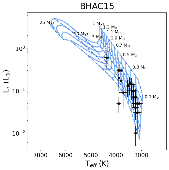
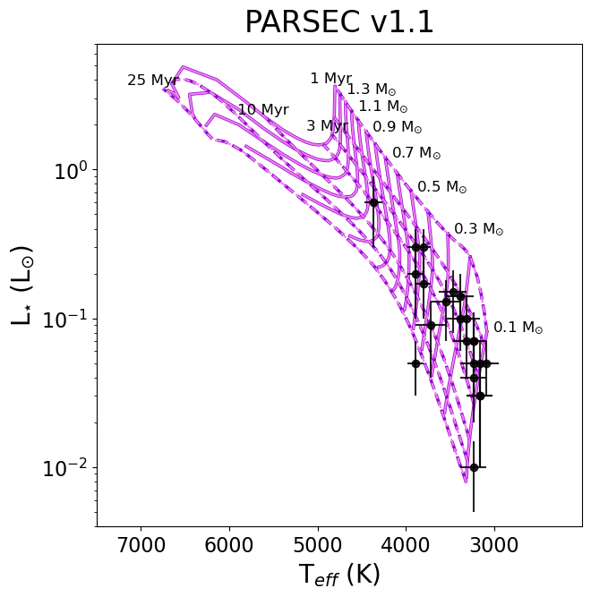
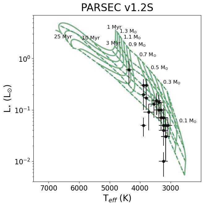
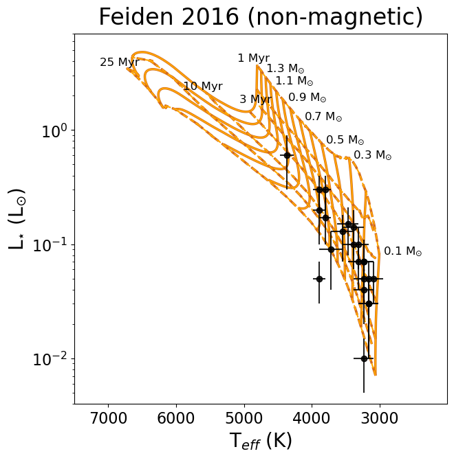
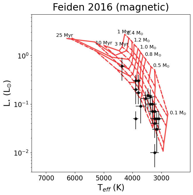
Figure 7: Isochronal age and mass contour lines for each of the five model sets considered in this paper. The mass and age ranges are 0.1 to 1.4 M_⊙ and 1 to 25 Myr in all panels. Black points show the L_⋆ and T_eff for our sample. Error bars come from the uncertainties listed in Table 1. The contours for each model are shown in a different color for ease of visual distinction; this color scheme is carried through all related figures for the rest of this paper. Top row: BHAC15 (Baraffe et al., 2015) (left, in blue), PARSEC v1.1 (Bressan et al., 2012) (center, in magenta), PARSEC v1.2S (Chen et al., 2014) (right, in green). Bottom row: non-magnetic models of Feiden (2016) (left, in orange), magnetic models of Feiden (2016) (center, in red).

To derive isochronal masses, we generate normal distributions in luminosity and temperature for each source. The peak values and widths of each distribution are the source’s L_⋆ and T_eff and their corresponding uncertainties, respectively (see Table 1). We then feed these normal distributions into the PMS tracks of each model set. This step is done with the pdspy package pdspy.stars, which interpolates linearly between grid points in each isochrone. The result is five distributions of isochronal mass for each target. In the following analysis, we use the median and scaled MAD of each distribution as mass and uncertainty, respectively, for each model. These isochronal masses are listed in Table 6. Table 7 shows minimum, maximum, median, and mean mass ratios (M_iso/M_dyn) for each set of tracks.

Table 6: Stellar Masses Derived from Evolutionary Tracks

Field	BHAC15a	PARSEC v1.1	PARSEC v1.2S	Feiden (2016), n-m	Feiden (2016), m
	(M⊙)	(M⊙)	(M⊙)	(M⊙)	(M⊙)
J15521088-2125372	0.18 (0.08)	0.11 (0.02)	0.23 (0.05)	0.17 (0.06)	0.22 (0.07)
J15530132-2114135	0.20 (0.08)	0.13 (0.04)	0.39 (0.10)	0.19 (0.08)	0.26 (0.09)
J15534211-2049282	0.26 (0.09)	0.16 (0.05)	0.5 (0.1)	0.24 (0.10)	0.3 (0.1)
J15562477-2225552	0.21 (0.08)	0.13 (0.04)	0.41 (0.10)	0.19 (0.08)	0.27 (0.09)
J16001844-2230114	0.17 (0.07)	0.12 (0.03)	0.37 (0.09)	0.15 (0.07)	0.23 (0.08)
J16014086-2258103	0.22 (0.08)	0.14 (0.04)	0.4 (0.1)	0.20 (0.08)	0.28 (0.10)
J16020757-2257467	0.3 (0.1)	0.25 (0.08)	0.6 (0.1)	0.3 (0.1)	0.5 (0.1)
J16035767-2031055	1.0 (0.1)	0.9 (0.1)	0.9 (0.1)	0.9 (0.1)	1.1 (0.2)
J16035793-1942108	0.4 (0.1)	0.28 (0.08)	0.6 (0.1)	0.4 (0.1)	0.6 (0.1)
J16062277-2011243	0.14 (0.06)	0.11 (0.02)	0.33 (0.09)	0.13 (0.05)	0.19 (0.07)
J16075796-2040087	0.5 (0.1)	0.3 (0.1)	0.64 (0.07)	0.5 (0.1)	0.6 (0.1)
J16081566-2222199	0.29 (0.09)	0.22 (0.07)	0.5 (0.1)	0.3 (0.1)	0.4 (0.1)
J16082324-1930009	0.65 (0.08)	0.52 (0.08)	0.71 (0.02)	0.66 (0.08)	0.8 (0.1)
J16090075-1908526	0.65 (0.09)	0.52 (0.07)	0.72 (0.01)	0.65 (0.09)	0.88 (0.08)
J16095933-1800090	0.21 (0.08)	0.14 (0.04)	0.4 (0.1)	0.20 (0.08)	0.28 (0.10)
J16104636-1840598	0.15 (0.06)	0.11 (0.02)	0.33 (0.09)	0.15 (0.06)	0.21 (0.08)
J16113134-1838259 B	0.70 (0.09)	0.57 (0.08)	0.72 (0.02)	0.7 (0.1)	0.99 (0.08)
J16115091-2012098	0.26 (0.09)	0.18 (0.06)	0.5 (0.1)	0.24 (0.09)	0.3 (0.1)
J16123916-1859284	0.56 (0.08)	0.45 (0.06)	0.70 (0.02)	0.57 (0.09)	0.83 (0.08)
J16142029-1906481	0.54 (0.06)	0.37 (0.07)	0.57 (0.08)	0.47 (0.08)	0.54 (0.06)
J16143367-1900133	0.3 (0.1)	0.20 (0.07)	0.5 (0.1)	0.3 (0.1)	0.4 (0.1)
J16163345-2521505	0.60 (0.07)	0.45 (0.07)	0.70 (0.02)	0.61 (0.08)	0.75 (0.09)
J16181904-2028479	0.16 (0.06)	0.11 (0.02)	0.33 (0.09)	0.15 (0.06)	0.21 (0.07)

5.2 Comparing Dynamical and Isochronal Masses

We compare isochronal versus dynamical masses for all sources in our sample for each of the five model sets. Scatterplots of M_iso versus M_dyn show a clear linear relationship between M_iso and M_dyn up to a mass of $\sim$1 M_⊙, and a shallowing of that relationship above 1 M_⊙. However, we also have very sparse data coverage above M_dyn $=$ 1 M_⊙, and it is unclear whether this shallowing is a true physical trend or simply an artifact of our current sampling. Additionally, a much larger fraction of our sources above 1 M_⊙ are known or candidate binary systems, which could also be contributing to this trend.

To account for these potential confounding factors, we perform a statistical analysis of dynamical versus isochronal masses for two cases: once for the full sample, and once for only those sources with M_dyn $\leq$ 1.0 M_⊙, where we have much better data coverage. This restriction excludes five sources: J15562477-2225552 (whose mass is an upper limit), J16035767-2031055 and J16142029-1906481 (discussed above), and J16075796-2040087 and J16113134-1838259 B (both of which have known or candidate companions). Statistics for both cases are presented in Table 7. We find that, in practice, our analysis is not meaningfully impacted by using the mass-limited sample versus the full sample. In this subsection, we discuss results for the M_dyn $\leq$ 1.0 M_⊙ sample only. Figures and a brief discussion for the full range of masses can be found in Appendix C.

In Figure 8, we show scatterplots of the isochrone-derived versus dynamical masses for each of the five sets of tracks for M_dyn $\leq$ 1.0 M_⊙. A 1:1 relationship is shown by a black solid line in all panels. We fit a line to the data in each panel using the scipy.odr package, which performs Orthogonal Distance Regression (ODR) fitting. The ODR method accounts for uncertainties in both the dependent (M_iso) and independent (M_dyn) variables. The best fit for isochronal versus dynamical mass is shown as a dashed, colored line in each panel.

We find that the non-magnetic Feiden (2016) models, BHAC15, and PARSEC v1.1 all consistently return lower masses than the dynamical mass, with slopes that do not agree with 1 within uncertainties (Fig. 8, top left, top center, and bottom left panel, respectively). The PARSEC v1.2S models, on the other hand, are about as likely to underestimate versus overestimate the dynamical masses. However, the overall slope of the trend is still very shallow and, unlike the other model sets, does not intersect the y-axis at zero (slope = 0.6$\pm$0.1, intercept = 0.2$\pm$0.0; see Fig. 8, top right panel).

In contrast, the magnetic models of Feiden (2016) agree very consistently with the dynamical mass results for M_⋆ $\leq$ 1 M_⊙ (Fig. 8, bottom center panel). The ODR best-fit line (slope = 1.0$\pm$0.1, intercept = 0.03$\pm$0.05) is consistent with a 1:1 relationship between the two methods within uncertainties, and the scatterplot shows no strong tendency toward over- or under-estimation by the magnetic models within this mass range.

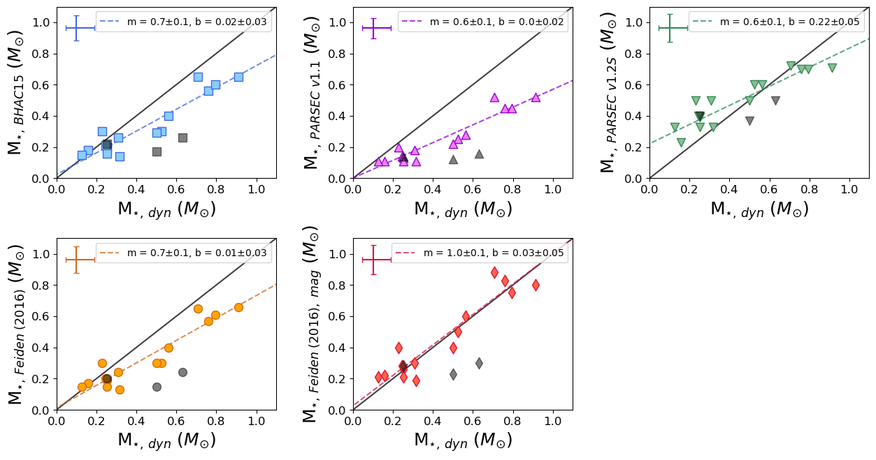
Figure 8: Comparison of stellar masses returned by each PMS evolutionary model set to the dynamical masses we derive using pdspy. The color scheme is the same as in Figure 7. In all panels, the isochronal mass is shown on the y-axis, and the dynamical mass (same in all cases) is shown on the x-axis. The black dotted line represents a 1:1 relation in all panels. The ODR best-fit line slope (m) and intercept (b) are listed in each panel. Top row: BHAC15 (left), PARSEC v1.1 (Bressan et al., 2012) (center), PARSEC v1.2S (Chen et al., 2014) (right). Bottom row: non-magnetic models of Feiden (2016) (left), magnetic models of Feiden (2016) (center). The significant improvement in agreement of the magnetic models of Feiden (2016) with the dynamical masses, as compared to the other PMS evolutionary models tested here, can be clearly seen in the bottom center panel. A figure covering the full range of masses can be found in Appendix C.

These results are also consistent with the isochronal- versus dynamical-mass ratios for each model set. Population-level statistics for these ratios (minimum, maximum, median, and mean) are presented in Table 7, columns 2-5. The BHAC15, PARSEC v1.1, and non-magnetic Feiden (2016) models all have minimum and maximum mass ratios 1.3-3.1$\times$ smaller than those of the PARSEC v1.2S and magnetic Feiden (2016) models, and their median and mean mass ratios typically do not agree with unity within uncertainties. In contrast, the magnetic Feiden (2016) tracks have both median and mean mass ratios within 2% of unity, with uncertainties comparable to those of the other models. The PARSEC v1.2S models, meanwhile, have median and mean mass ratios larger than unity by $\geq$11%, i.e., they are more likely to overestimate mass than to underestimate it. The uncertainties on the PARSEC v1.2S median and mean are also notably larger than the uncertainties for any other model set.

We also calculate Spearman $\rho$ correlation coefficients between the dynamical masses and the M_iso/M_dyn mass ratios. These coefficients are listed in columns 6 and 7 of Table 7. We consider a correlation to be significant if it has a p-value less than 6.3$\times$10^-5 (corresponding to $\geq$ 4$\sigma$ significance assuming normally-distributed data). All model sets have a negative correlation between mass ratio and dynamical mass, but only the PARSEC v1.2S models have a p-value that indicates statistical significance. Both the highly-negative correlation coefficient ($\rho$ $=$ -0.84) and small p-value ($>$4$\sigma$) indicate that the accuracy of the PARSEC v1.2S models varies with mass in a statistically-significant way. This is consistent with Figure 8, in which the data for PARSEC v1.2S have relatively little scatter but clearly do not follow a 1:1 line. Rather, PARSEC v1.2S is highly likely to overestimate stellar mass for M_dyn $\lesssim$0.6 M_⊙, and underestimate it for M_dyn $\gtrsim$0.6 M_⊙.

Table 7: Sample Statistics for Isochronal vs. Dynamical Masses

	Mass Ratio (Miso/Mdyn)				Miso/Mdyn  vs  Mdyn		Miso  vs  Mdyn
PMS Model Set	Min	Max	Median	Mean	$\rho^{a}$	p	Db	p
M⋆ $\leq$ 1.0 M⊙ Onlyc
BHAC15	0.34	1.31	0.75 (0.22)	0.77 (0.26)	$-$0.51	0.03	0.33	0.3
PARSEC v1.1	0.24	0.87	0.56 (0.15)	0.55 (0.17)	$-$0.28	0.3	0.56	7$\times$10-3
PARSEC v1.2S	0.74	2.62	1.11 (0.47)	1.30 (0.49)	$-$0.84	1$\times$10-5	0.44	0.06
Feiden (2016), non-magnetic	0.30	1.31	0.75 (0.23)	0.75 (0.26)	$-$0.48	0.04	0.39	0.1
Feiden (2016), magnetic	0.46	1.75	1.00 (0.23)	1.02 (0.34)	$-$0.49	0.04	0.22	0.8
Full Sampled
BHAC15	0.25	1.31	0.71 (0.27)	0.69 (0.29)	$-$0.69	4$\times$10-4	0.32	0.2
PARSEC v1.1	0.15	0.87	0.51 (0.17)	0.49 (0.19)	$-$0.56	7$\times$10-3	0.45	0.02
PARSEC v1.2S	0.23	2.62	1.03 (0.53)	1.13 (0.58)	$-$0.91	4$\times$10-9	0.36	0.1
Feiden (2016), non-magnetic	0.23	1.31	0.72 (0.26)	0.67 (0.29)	$-$0.68	5$\times$10-4	0.32	0.2
Feiden (2016), magnetic	0.28	1.75	0.95 (0.36)	0.91 (0.39)	$-$0.69	4$\times$10-4	0.18	0.9

In order to more fully quantify the similarity of the isochrone-derived and dynamical masses, we employ the 2-sample Kolmogorov-Smirnov (KS) test. The KS test quantifies how likely two sample distributions are to have been drawn from the same parent distribution. The KS test statistic (D) is a measure of the maximum distance between the Cumulative Distribution Functions (CDFs) of the two samples, and its p-value represents the statistical likelihood of the null hypothesis (here, that the two samples were drawn from the same parent distribution). The KS test statistics and p-values for our sample are shown in the last two columns of Table 7. Figure 9 shows the CDFs used in the KS tests.

Our KS test results confirm that the magnetic tracks of Feiden (2016) show the smallest difference with our dynamical masses (D$=$0.22). However, it must be noted that none of the PMS models have a p-value that explicitly rejects the null hypothesis with $\geq$4$\sigma$ confidence (p $\leq$ 6.3$\times$10^-5). This is consistent with the generally correlated, but rarely 1:1, isochronal versus dynamical masses shown in Figure 8.

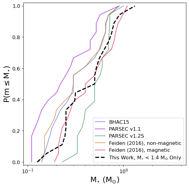
Figure 9: Cumulative distribution functions (CDFs) of stellar mass for the five PMS evolutionary models considered in this work, along with the dynamical masses we derive using pdspy. In this Figure, we include only those sources whose dynamical mass is $\leq$1 M_⊙. A figure showing CDFs using the full sample can be found in Appendix C.

Taken together, the ODR best-fit line, mass-ratio, Spearman $\rho$, and KS-test results suggest the magnetic models of Feiden (2016) are the most reliable isochronal method of determining stellar masses in the M_⋆ $\leq$ 1 M_⊙ mass range, for our 5-11 Myr targets.

5.3 Comparison with Literature Results

To place our results in broader context, we compare our findings to the dynamical-isochronal mass comparisons of Rizzuto et al. (2016), Simon et al. (2019), and Braun et al. (2021).

Rizzuto et al. (2016) use astrometric measurements to derive the orbital and stellar properties of seven binary pairs, six of which are in Upper Sco: J15500499-2311537, J15573430-2321123, J16015822-2008121, J16051791-2024195, J16081474-1908327, and J16245136-2239325. They compare these dynamical results to those of the Padova models of Girardi et al. (2002), the Dartmouth models of Dotter et al. (2008), and the BT-Settl models of Allard et al. (2011). Rizzuto et al. (2016) find that the isochronal and dynamical masses agree within uncertainties for the G-type stars in their sample. However, the isochronal masses for the M-type stars are highly model-dependent. The Girardi et al. (2002) models significantly overestimate mass for the M stars in their sample, and the Dotter et al. (2008) and Allard et al. (2011) models consistently underestimate mass by 0.2$-$0.4 M_⊙.

Simon et al. (2019) use CO line data in disks to derive dynamical masses for 29 stars in Taurus and 3 in Ophiuchus. They use the DiskFit package (Piétu et al., 2007) to fit a power-law disk model to the CO, assuming a vertically-isothermal temperature structure and imposing a CO depletion zone near the disk midplane. They compare these dynamical masses to those derived from the BHAC15 and the magnetic Feiden (2016) models, and find that the non-magnetic models typically underestimate stellar mass by approximately 30%. In contrast, the magnetic models of Feiden (2016) have a typical difference of only 0.01$\pm$0.02 M_⊙ with the dynamical masses.

In a separate study, Braun et al. (2021) derive masses for 45 pre-main sequence stars in Taurus and Lupus (17 in Taurus, 28 in Lupus) using Doppler-shifted, stacked ¹²CO, C¹⁸O, and CN line data. They follow the method detailed in Yen et al. (2016, 2018), which is similar to a Keplerian masking approach and assumes 1) a thin disk geometry and 2) identical excitation conditions for all line emission. Braun et al. (2021) compare their dynamical masses to the five model sets we consider in this work, plus those of Palla & Stahler (1993) and Siess et al. (2000). Based on the mean difference between isochronal and dynamical masses in three discrete mass bins (M_⋆ $\leq$ 0.6 M_⊙, 0.6 $\leq$ M_⋆ $\leq$ 1.3 M_⊙, M_⋆ $\geq$ 1.3 M_⊙), they conclude that the magnetic models of Feiden (2016) agree well with dynamical masses for intermediate-mass sources but tend to overestimate stellar masses for the lowest-mass sources (M_⋆ $\leq$ 0.6 M_⊙).

Overall, our findings agree well with the literature: the isochronal masses for PMS stars are highly model-dependent but, on the whole, non-magnetic models tend to return lower values than our dynamical masses by $\gtrsim$25% (median absolute differences of $\gtrsim$0.13 to 0.2 M_⊙, see Table 7). The exception is, as noted above, the PARSEC v1.2S model set, which is slightly more likely to overestimate dynamical masses than underestimate them. In contrast, the magnetic models of Feiden (2016) tend to return masses that are in good agreement with the dynamical masses (median 2% relative difference, median 0.0001 M_⊙ absolute difference; see Table 7, Figure 8, Figure 9). These trends suggest that the majority of non-magnetic isochronal methods may be consistently underestimating stellar mass for low-mass PMS stars by $\gtrsim$25%.

In contrast with the results of Braun et al. (2021), we do not find that the magnetic Feiden (2016) models overestimate stellar mass for sources with M_dyn $\leq$ 0.6 M_⊙. This is likely due to the difference in modeling methods between these two works. Our approach includes dynamical modeling of both spatial and spectral components of the gas lines and does not assume a uniform, thin disk structure, in contrast to Braun et al. (2021). This possibility is supported by Braun et al. (2021) themselves, who note discrepancies between the dynamical masses they derive and those derived by Simon et al. (2019) for the 11 sources common to both samples; Simon et al. (2019) use Keplerian disk fitting, in contrast to the line-stacking approach of Braun et al. (2021).

Finally, the work we present herein extends the evaluation of isochronal PMS masses to the 5-11 Myr age range, complementing existing work in younger star-forming regions (e.g. Taurus, 1-3 Myr; Simon et al., 2019). The consistency of our results with those of younger regions suggests that the improved performance of magnetic over non-magnetic models is consistent for stellar ages up to $\sim$11 Myr.

5.4 The Potential Impact of Starspots

One potential complication in the evaluation of stellar evolutionary models’ performance is the presence of starspots. Strong magnetic activity at or near the stellar surface can create large, cool starspots over a significant fraction ($\geq$10%) of the stellar surface of low-mass stars (e.g. Rydgren & Vrba, 1983; Bary & Petersen, 2014; Somers & Pinsonneault, 2015). This can complicate both stellar spectral typing and inferred masses: starspots can push a star’s derived T_eff values lower which, when combined with stellar isochrones, will yield comparatively lower stellar masses. Somers & Pinsonneault (2015), for example, suggest that starspots can lead to isochrone-based masses being underestimated by up to a factor of two.

Flores et al. (2022) examine the impact of starspots on a star’s derived T_eff in both the optical and near-infrared regimes, and explore whether this translates to a systematic bias in isochrone-inferred masses. They examine the spectra of 40 young stars in Taurus-Auriga and Ophiuchus, and find that starspots have a greater impact on optical temperatures than infrared temperatures. This results in a greater discrepancy between isochronal and dynamical masses when optically-derived T_eff are used than when infrared-derived T_eff are used. Similarly, Pérez Paolino et al. (2024) explore the impact of starspots on the near-infrared spectra of 10 T-Tauri stars in Taurus-Auriga. They find that correcting for starspots results in median stellar mass increases of $+$0.24 and $+$0.44 M_⊙ (34% and 88%, respectively) relative to masses derived from uncorrected optical and near-infrared spectra. Feiden (2016) also consider starspots, both as a potential additional factor in isochronal fitting and as a separate, alternate explanation for the mass and age discrepancies noted in the literature (Preibisch & Mamajek, 2008; Pecaut et al., 2012). They note that the difference in scale between the magnetic fields involved in the production of starspots (localized) versus those in their magnetic models (global) will manifest as differences in the photometric properties of each star. In the limit that starspots cover a large fraction of the stellar surface, the two explanations should produce convergent results.

Sufficient data do not yet exist to robustly distinguish between the starspot and global-magnetic inhibition possibilities. Likewise, a full comparison of the starspot and disk dynamical methods is beyond the scope of this paper. However, we do compare the impact of these methods on derived stellar ages in our companion paper, Towner et al. (2025b, in prep).

5.5 M_disk vs. M_⋆

Given the widespread use of isochronal masses and the known dependence of isochronal mass on the specific model, it is worth considering whether known M_⋆-dependent relations still hold when dynamical masses are used instead. In this section, we consider the relationship between log(M_disk) and log(M_⋆), and evaluate whether it depends on the use of isochronal versus dynamical masses. This comparison covers the full mass range of the sample, but excludes the sources for which we derive upper limits on disk mass and/or stellar mass.

The relationship between stellar mass and disk dust mass has been observed in numerous young star-forming regions Andrews et al. (e.g. Taurus, 1-2 Myr; Lupus, 1-3 Myr; Chameleon I, 2-3 Myr; 2013); Pascucci et al. (e.g. Taurus, 1-2 Myr; Lupus, 1-3 Myr; Chameleon I, 2-3 Myr; 2016), and has been found to be approximately linear: log(M_dust) $\propto$ log(M_⋆). However, recent observations suggest that the log(M_disk)$-$log(M_⋆) relation may steepen with time. Barenfeld et al. (2016) find a slope of 1.67$\pm$0.37 for the older Upper Scorpius region assuming a dust temperature that scales with stellar luminosity, and Pascucci et al. (2016) find slopes of 1.9$\pm$0.4 (assuming L_⋆-scaled T_dust) to 2.7$\pm$0.4 (assuming constant T_dust $=$ 20 K). This steepening of the M${}_{dust}-$M_⋆ relation has been interpreted as a depletion of millimeter-size dust grains at larger radii as protoplanetary disks evolve (Barenfeld et al., 2016; Pascucci et al., 2016). However, the precise mechanism of this depletion remains an open question.

Following the methods of Barenfeld et al. (2016) and Pascucci et al. (2016), we derive disk dust masses for our targets using the equation

$$M_{d}=\frac{S_{\nu}d^{2}}{\kappa_{\nu}B_{\nu}(T_{d})},$$ (8)

where $S_{\nu}$ is our measured continuum flux density at 870 $\mu$m, $d$ is the Gaia-derived distance to each source, $\kappa_{\nu}$ is the dust opacity, and $T_{d}$ is the dust temperature. We assume a dust opacity of $\kappa_{\nu}$ $=$ 2.7 cm² g^-1 at 345 GHz, where $\kappa_{\nu}$ $=$ 2.3 cm² g^-1 at 230 GHz and scales with frequency as $\nu^{0.4}$ (Barenfeld et al., 2016).

We derive these masses under two different assumptions for dust temperature: T_dust $=$ 20 K, and T_dust $=$ 25 K $\times$ (L_⋆/L_⊙)^0.25 (Andrews et al., 2013; Pascucci et al., 2016). Table 8 lists the integrated continuum flux densities and the disk dust masses derived for each source. The continuum flux densities were obtained from the deconvolved fit results of CASA’s imfit task unless otherwise noted. The imfit task fits a 2D Gaussian to each source in the image plane. We verified each fit with a by-eye examination of the residual image. Sources with peak residuals above 3$\sigma$ were refit. If no good fit could be obtained, we performed manual aperture photometry for the source instead.

Table 8: Disk Dust Masses

Field	S${}_{870~\mu m}^{a}$	M${}_{T_{scale}}$	M${}_{T_{20\,K}}$
	(mJy)	(M⊕)	(M⊕)
J15521088-2125372	0.4 (0.2)	0.8 (0.3)	0.14 (0.07)
J15530132-2114135	5.2 (0.1)	3.7 (0.1)	1.40 (0.06)
J15534211-2049282	2.7 (0.2)†	1.3 (0.1)	0.62 (0.06)
J15562477-2225552	$<$ 0.30	$<$ 0.18	$<$ 0.08
J16001844-2230114	3.6 (0.1)	2.0 (0.3)	0.9 (0.1)
J16014086-2258103	3.2 (0.1)	1.26 (0.05)	0.62 (0.02)
J16020757-2257467	4.4 (0.1)	1.60 (0.05)	1.09 (0.03)
J16035767-2031055	5.2 (0.1)	1.16 (0.03)	1.33 (0.03)
J16035793-1942108	1.4 (0.2)	0.7 (0.1)	0.44 (0.06)
J16062277-2011243	0.4 (0.1)	0.27 (0.07)	0.11 (0.03)
J16075796-2040087	19.1 (0.2)†	11.0 (0.9)	6.0 (0.5)
J16081566-2222199	1.1 (0.1)	0.41 (0.04)	0.27 (0.03)
J16082324-1930009	36.6 (0.3)†	11.5 (0.2)	8.7 (0.2)
J16090075-1908526	41.4 (0.3)†	11.0 (0.2)	9.8 (0.2)
J16095933-1800090	0.38 (0.08)	0.18 (0.04)	0.09 (0.02)
J16104636-1840598	2.0 (0.1)	1.6 (0.1)	0.51 (0.03)
J16113134-1838259 B	86 (2)	26 (2)	27 (2)
J16115091-2012098	0.6 (0.1)	0.30 (0.05)	0.17 (0.03)
J16123916-1859284	6.7 (0.2)	1.83 (0.07)	1.63 (0.06)
J16142029-1906481	33.2 (0.3)†	20.9 (0.7)	8.5 (0.3)
J16143367-1900133	1.3 (0.1)	0.57 (0.05)	0.33 (0.03)
J16163345-2521505	2.4 (0.2)	1.1 (0.1)	0.80 (0.07)
J16181904-2028479	3.5 (0.1)	2.5 (0.1)	0.84 (0.04)

Figure 10 shows scatterplots of log(M_disk) versus log(M_⋆) for our data. The dynamical stellar masses are shown in black, and the BHAC15 stellar masses are shown in blue. The left-hand panel shows results under the luminosity-scaled T_dust assumption, and the right-hand panel shows results assuming T_dust $=$ 20 K. We derive a log(M_disk)$-$log(M_⋆) relation using Orthogonal Distance Regression (ODR) fitting for both our dynamical masses and the BHAC15 M_⋆ values. Under the luminosity-scaled temperature assumption, we derive the relation

$$log(M_{disk})=(2.8\pm 0.6)log(M_{\star})+(1.0\pm 0.3)$$ (9)

using our dynamical masses, with Spearman $\rho$ $=$ 0.50 and a p-value of 0.02. Using the BHAC15 masses and the scaled-temperature assumption, we derive

$$log(M_{disk})=(3.3\pm 1.2)log(M_{\star})+(1.9\pm 0.7)$$ (10)

with Spearman $\rho$ $=$ 0.39 and a p-value of 0.08.

Under the constant-T_dust assumption, we derive

$$log(M_{disk})=(2.8\pm 0.5)log(M_{\star})+(0.9\pm 0.2).$$ (11)

using our dynamical masses (Spearman $\rho$ $=$ 0.71, p $=$ 2$\times$10^-4), and

$$log(M_{disk})=(3.4\pm 0.9)log(M_{\star})+(1.7\pm 0.5).$$ (12)

using the BHAC15 masses (Spearman $\rho$ $=$ 0.65, p $=$ 1$\times$10^-3).

All Spearman $\rho$ values show a moderate correlation between M_⋆ and M_disk, with associated p-values between corresponding to $\leq$4$\sigma$. The p-values for the constant-T_dust cases are lower than those for the scaled-T_dust cases (corresponding to $\gtrsim$3$\sigma$), which would seem to indicate a more statistically-significant correlation. However, it is possible this increased significance is actually a consequence of assuming the same T_dust for all disks, rather than a reflection of real physics.

Regardless of the method used, we derive a relationship between log(M_disk) and log(M_⋆) that is steeper than linear within the uncertainties of the ODR fit. Our derived slopes are consistent with those of Pascucci et al. (2016) within the relevant uncertainties, and steeper than Barenfeld et al. (2016) in all cases. The discrepancy with Barenfeld et al. (2016) is likely due to their use of a continuum-selected sample in contrast to our (more gas-rich) CO-selected sample. The different methodologies in deriving the best-fit line and the inclusion of upper-limit disk masses in the Barenfeld et al. (2016) calculation (48 out of their 106 data points) may also be contributing.

The steeper-than-linear relationship we derive for Upper Sco is consistent with the theory that the millimeter-size dust content of protoplanetary disks evolves with time, either through inward radial drift of the millimeter dust or grain growth to larger sizes (Pascucci et al., 2016). While we lack the spatial resolution and spectral coverage in this work to distinguish between these two possibilities, an exploration of grain growth in Upper Sco will be the subject of future work.

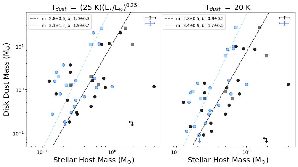
Figure 10: Disk dust mass (see Table 8) versus stellar mass for the 23 sources in our sample. Upper limits on dust masses are marked with downward arrows. Upper limits on stellar mass are marked with left-facing arrows. In both panels, the black points denote the stellar masses we derive via Keplerian fitting, and the blue points denote stellar masses derived from the best-fit BHAC15 PMS models using L_⋆ and T_eff. Left panel: Disk mass versus stellar mass assuming the disk dust temperature scales as 25 K (L_⋆/L_⊙)^0.25. The best-fit lines using the dynamical and BHAC15 stellar masses are shown in black and blue, respectively; the best-fit slope (m) and intercept (b) for each case are shown in the upper left-hand corner. Median uncertainties are shown as error bars in the upper right-hand corner. Right panel: As for the left-hand panel, except the disk dust masses were calculated assuming a constant dust temperature of 20 K.

Under both temperature assumptions, the slope of the log(M_disk)$-$log(M_⋆) relation is steeper when derived using the BHAC15 masses than when using the dynamical masses. This could suggest that the use of dynamical masses will shallow the slope of the log(M_disk)$-$log(M_⋆) relation. This would be consistent with our finding that dynamical methods tend to return slightly higher stellar masses ($\gtrsim$25%) than isochronal methods. However, the BHAC15 and dynamical-mass slopes always agree with each other within uncertainties. Therefore, we do not consider this trend to be statistically significant at this time.

We also find no change in slope with the T_dust assumption. This is in conflict with Pascucci et al. (2016), who note a clear shallowing of the relation with luminosity-scaled T_dust (1.9$\pm$0.4) as compared to a constant T_dust (2.7$\pm$0.4). This discrepancy may be a result of our comparatively smaller sample size, though we do note that our uncertainties on the slopes derived using dynamical masses ($\pm$0.5 to 0.6) is comparable to those derived by Pascucci et al. (2016) and Barenfeld et al. (2016). It is also possible that, because the disks in our sample are larger and more CO-rich than in most continuum-based samples, our disk temperatures may be naturally closer to 20 K to begin with; in that case, the use of the constant T_dust $=$ 20 K would have less of an impact on our best-fit line.

5.6 Potential Sources of Additional Uncertainty

We have already examined our data for signs that the CO data are tracing outflows rather than disk rotation, and found no evidence of outflow contamination (§ 2.4). In this section, we explore two further potential sources of contamination or bias in the data: sources with known or candidate companions, and bias in stellar mass with inclination angle. We describe the full details of this examination in Appendix D.

In short, we find little evidence for strong effects due to the inclusion of binary sources. In general, excluding the known or candidate binaries from our sample drops the correlations between mass ratio and dynamical mass to below 3$\sigma$ significance. The one exception is the strong correlation for the PARSEC v1.2S models, which remain at $>$5$\sigma$ significance regardless of the exclusion of the binary sources. Given the smaller number of sources in the binary-excluded sample, and the relatively low statistical significance of most of these relations to begin with, these results are not surprising.

To test for methodology-induced bias in stellar mass with disk inclination angle, we compare our M_⋆ and $i$ to the stellar masses of Barenfeld et al. (2016) and the CO- and continuum-derived disk inclination angles of Barenfeld et al. (2017). All median $i$ and M_⋆ values agree within their respective uncertainties. We perform additional KS tests, and find that there is no statistically significant ($>$3$\sigma$) difference between the samples in either M_⋆ or $i$. We therefore conclude that the pdspy-derived dynamical masses have not introduced any additional bias in mass with inclination angle.

6 Summary

We have derived the masses of 23 pre-main sequence K- and M-type stars with disks in Upper Scorpius using a Keplerian disk model and the open-source package pdspy. We successfully fit the ¹²CO J$=$3$-$2 emission for 22 out of 24 sources (Table 4), and fit the ¹³CO J$=$3$-$2 emission for 4 out of the 6 sources with $>$5$\sigma$ ¹³CO emission (Table 5). We also jointly fit the ¹²CO$+$¹³CO emission for the three sources with $>$5$\sigma$ emission in both lines (Table 5). We find a median sample mass of 0.5 M_⊙, and a minimum and maximum mass of 0.13${}^{+0.07}_{-0.05}$ M_⊙ and 4.0${}^{+4.0}_{-2.0}$ M_⊙, respectively.

We have evaluated the best-fit values and uncertainties produced by pdspy using both a $\chi^{2}_{min}$+$\Delta\chi^{2}$ method and a median plus standard deviation method. We find that the median$+$standard deviation method is prone to underestimating parameter uncertainties. We report as our best-fit results the values corresponding to the minimum $\chi^{2}$ fit, and uncertainties corresponding to the maximum and minimum values within $\Delta\chi^{2}$ $=$ 15.975.

We have extensively compared our results to those of five pre-main sequence evolutionary model sets: BHAC15 (Baraffe et al., 2015), PARSEC v1.1 (Bressan et al., 2012), PARSEC v1.2S (Chen et al., 2014), and both the standard and magnetic models of Feiden (2016). We perform this comparison for both the full sample and for only those sources with 0.1 M_⊙ $\leq$ M_⋆ $\leq$ 1 M_⊙. We find the following:

1. The magnetic models of Feiden (2016) are in very good agreement with our dynamical results for M_⋆ $\leq$1 M_⊙. They have a nearly 1:1 relationship with the dynamical masses up to 1 M_⊙, and Kolmogorov-Smirnov tests comparing dynamical and isochronal masses for all five model sets show that the magnetic models are in the best agreement by far with our dynamical masses.

2. The BHAC15, PARSEC v1.1, and non-magnetic Feiden (2016) models all tend to underestimate dynamical mass by $\gtrsim$25% (Figure 8, Table 7). In contrast, the PARSEC v1.2S models tend to overestimate dynamical masses for M_dyn $\lesssim$0.6 M_⊙ and overestimate dynamical masses for M_dyn $\gtrsim$0.6 M_⊙.

3. In most cases, model accuracy (as measured by the ratio of the PMS to dynamical-mass results) is not correlated with stellar mass at the $>$4$\sigma$ level. The exception is the PARSEC v1.2S models, which have a $\gtrsim$5$\sigma$ negative correlation between dynamical mass and the M_iso/M_dyn ratio. This indicates that the accuracy of the PARSEC v1.2S models as compared to the dynamical masses is mass-dependent.

4. We find no indication that the magnetic models of Feiden (2016) have a tendency to overestimate mass for the lowest-mass sources (M_⋆ $\lesssim$ 0.6 M_⊙). This is in contrast with the literature findings of Braun et al. (2021). We suggest that this contrast is due to a difference in the methods used to derive dynamical mass.

5. We find that the sample statistics and our overall interpretation are not meaningfully different when considering the full sample as opposed to the mass-limited sample, or when including versus excluding sources with known or candidate companions. The magnetic models of Feiden (2016) are clearly the best match to our dynamical masses in all cases.

This work, performed with a comparatively large sample (23 sources) on a 5-11 Myr old region, complements similar work on younger regions (e.g. Taurus, 1-3 Myr; Simon et al., 2019). Our findings extend the systematic evaluation of stellar evolutionary models’ performance - and in particular, the consistently superior performance of magnetic models over non-magnetic ones - up to ages of $\sim$11 Myr.

We derive the log(M_disk)$-$log(M_⋆) relationship for our data, and find a steeper-than-linear relationship regardless of the M_disk and M_⋆ values used. This is consistent with the existing literature, which finds slopes $>$ 1.0 within uncertainties for Upper Sco (Barenfeld et al., 2016; Pascucci et al., 2016). This steeper slope is in contrast with younger regions such as Taurus (Andrews et al., 2013), and has been interpreted as indicating either grain growth or inward radial drift of the millimeter-size grains in older disks.

We also find that using dynamical masses as opposed to isochronal masses tends to produce shallower derived slopes for the log(M_disk)$-$log(M_⋆) relation, but that the values still agree with each other within uncertainties. We suggest that future studies with larger sample sizes will be able to explore this possibility with greater statistical significance. We also find no difference in slope between two different T_dust assumptions, which contradicts the findings of Pascucci et al. (2016). This may be a consequence of our comparatively gas-rich sample as compared to previous studies.

We investigate our results for potential bias due to the presence of binary sources or other nearby companions, and find no significant impact on our results. We also test for correlations between stellar mass and inclination angle, and find no statistically-significant difference between our sample and those of Barenfeld et al. (2016) and Barenfeld et al. (2017). We conclude that our disk-modeling procedure has not introduced any mass-versus-inclination bias into our results.

Overall, the magnetic PMS evolutionary tracks of Feiden (2016) provide by far the most consistent results with our dynamical masses. We conclude that, in the absence of direct dynamical measurements, the magnetic Feiden (2016) models are the most accurate and reliable isochronal method for determining the masses of late-type (M_⋆ $\leq$ 1 M_⊙) pre-main sequence stars within the 5-11 Myr age range of our sample.

Appendix A Additional Figures for SED and pdspy Fitting

A.1 BT Settl Fitting Procedure and Best-fit SEDs

We derive L_⋆ using BT Settl atmospheric models for two reasons. First, the L_⋆ derived by Barenfeld et al. (2016) were published before the first Gaia data release, and assume a single distance of 145 pc for all sources. Given the importance of precise Gaia distances to our dynamical mass derivations, it was necessary to re-derive luminosities using the new Gaia distances. This ensures that, when comparing dynamical with isochronal masses, we are comparing like with like. Second, in the course of revising L_⋆ to account for revised distances, we discovered that at least 6 sources (1/4 of the sample) appear to have excess emission in the 2MASS J-band data as compared to the optical photometry. This meant that replicating the procedure of Barenfeld et al. (2016), who derive L_⋆ using J-band photometry and a bolometric correction, was likely to yield spurious results for some sources.

For each source except J16113134-1838259 A & B (see § 2.2), we fit data from each of the following, as available: Gaia Data Release 3 (DR3; Gaia Collaboration et al., 2021), the AAVSO Photometric All-Sky Survey (APASS; Henden & Munari, 2014; Henden, 2019), the Panoramic Survey Telescope and Rapid Response System (Pan-STARRS; Flewelling et al., 2020), the Deep Near-Infrared Survey of the Southern Sky (DENIS; DENIS Consortium, 2005), and the Two Micron All-Sky Survey (2MASS; Skrutskie et al., 2006). Further details of each dataset can be found at the end of this section.

Our fit parameters are as follows: we fix the BT Settl model temperature to the T_eff listed in Table 1, rounded to the nearest hundred (the precision of the BT Settl models). We assume Solar metallicity values with no $\alpha$ enhancement. We allow log(g) to vary between 3.0 and 4.5; this range was chosen based on the typical masses and radii for sources of this type and age. The BT Settl model grid moves in steps of 0.5 for log(g). We fit our OIR photometry data to the BT Settl models over our own grid in A_V and $\theta$, where A_V is the visual extinction, $\theta$ $=$ R_⋆/$d$ is the apparent size of the source on the sky, and $d$ is the Gaia distance to the source. The allowed A_V values range from 0 to 4.5 in steps of 0.1, and the allowed $\theta$ values range from 1$\times$10^-6 arcseconds to 8$\times$10^-5 arcseconds in steps of 0.25$\times$10^-6.

For each source, we read in the OIR photometry and convert it from magnitudes to flux density in Janskys using either the zero-point values reported in the literature for each facility and filter (see below), or a zero-point flux of 3631 Jy if the reported magnitude uses the AB system. We de-redden our data for each A_V grid point using the extinction laws of Wang & Chen (2019); for filters not directly listed in Wang & Chen (2019), we determine A_λ using linear extrapolation from the nearest listed wavelengths. To compare our model photometry to our observed photometry, we calculate the mean specific flux density of the model (S_ν, in units of erg s^-1 cm^-2 sr^-1 Hz^-1) within the frequencies corresponding to 50% of the maximum transmission level of each filter. This value is then scaled according to $\theta$ for each grid point. We calculate $\chi^{2}$ for each fit using the measurement and flux calibration uncertainties of the catalog photometry (see below), the uncertainties on each A_λ reported by Wang & Chen (2019), and an additional 10% uncertainty to account for potential variability in these low-mass pre-main sequence stars. We determine the best-fit model by minimizing $\chi^{2}$.

The best-fit A_V is fit directly. The best-fit R_⋆ is derived using R_⋆ $=$ $\theta_{best}d$, where $\theta_{best}$ is the best-fit $\theta$ value in arcseconds and $d$ is the Gaia distance to the source. L_⋆ is derived by integrating the best-fit model SED over frequency space and then multiplying by 4$\pi$R${}_{\star}^{2}$. The uncertainties on A_V, R_⋆ and L_⋆ are calculated using the same $\Delta\chi^{2}$ method described in § 3.4. For a 3-parameter fit, the interval corresponding to a 1$\sigma$ uncertainty is $\Delta\chi^{2}$ $=$ 3.52675.

In Figure 11, we show the best-fit BT Settl model for each source in red, with the de-reddened optical and infrared photometry shown in black. Vertical error bars show the uncertainties (including the additional 10% to account for variability) used in the fit. Horizontal “error” bars show the range of wavelengths covered by each band, as defined by the 50%-of-maximum transmission level used for fitting (see above). In Table 9, we report the best-fit parameters for each source, along with the specific photometric data used for each fit. We also list the luminosities in Table 1.

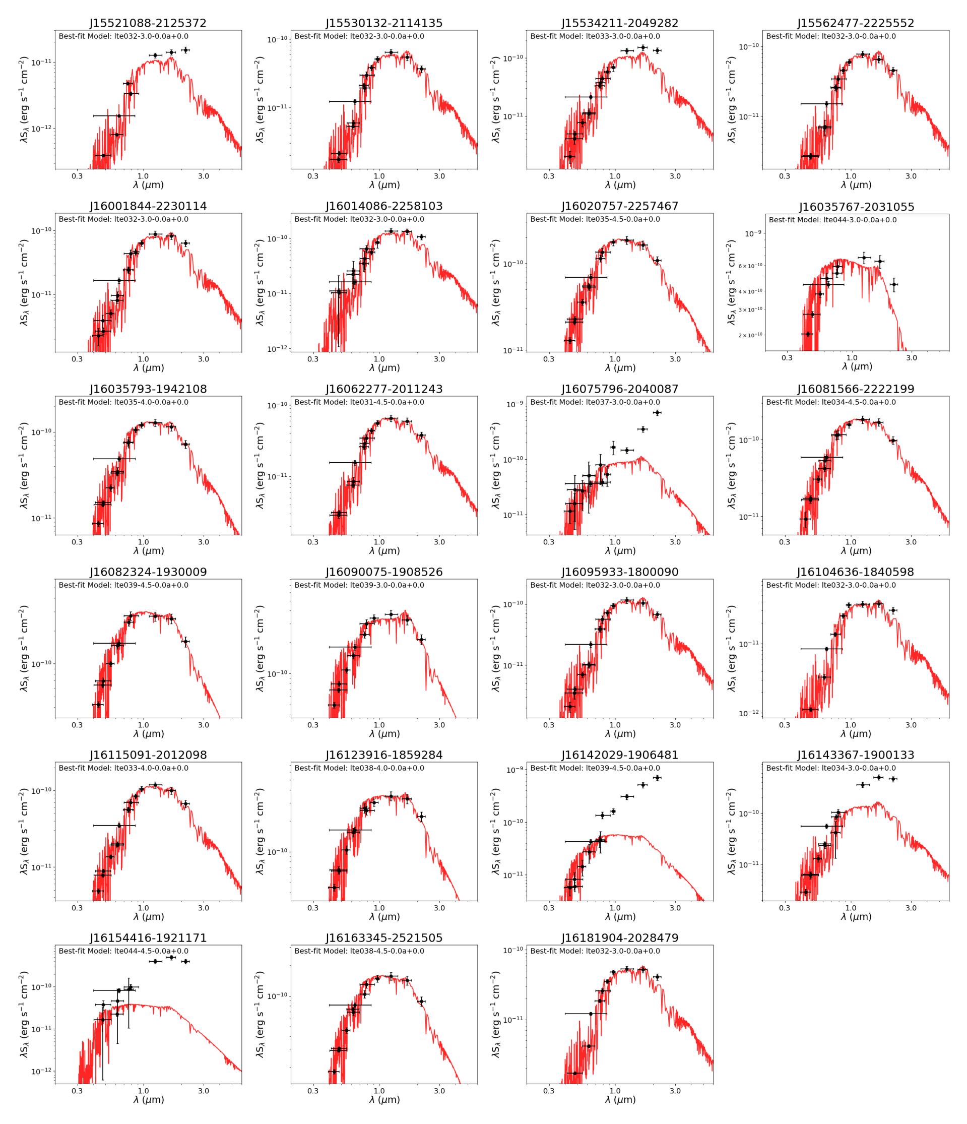
Figure 11: Optical-infrared photometry (black points) and best-fit BT Settl models (red curves) for 23 sources fit with BT Settl models (J16113134-1838259 A & B were not excluded; see § 2.2). The y-axis error bars are the uncertainties used in the fit, and the x-axis “error” bars show the wavelength ranges used to calculate the model S_ν for each observing band ($\geq$50% of maximum transmission; see text). The best-fit parameters for each source are listed in Table 9.

Some sources exhibit notable near-infrared excess, which is not unusual for pre-main sequence, disk-bearing targets such as these. In these cases, the fits more closely trace the optical data (dominated by the stellar photosphere) than the near-infrared data (potentially dominated by thermal emission from the disk). This is a consequence of both the larger number of data points in the optical regime and their relative uncertainties, which are typically smaller than for the 2MASS data. As a sanity check, we ran test fits in which we downweight the 2MASS data for sources with infrared excess. We found that the downweighted fits produced the same L_⋆ values as the standard fits within uncertainties. In light of this finding and for internal consistency, we use the standard fit results for all sources.

All but three of these sources are classified as either Classical T-Tauri (CTT) or Weak T-Tauri (WTT) in the Konkoly Optical YSO Catalog (KYSO), which was compiled by cross-referencing Gaia DR3 and literature data (Marton et al., 2023). The remaining three sources (J15521088-2125372, J15534211-2049282, and J16014086-2258103) are not listed in the KYSO catalog. Of the 20 listed sources, 16 have specific variability types listed, which were defined and identified for Gaia data in Rimoldini et al. (2023) and Gavras et al. (2023). Most of our sources are classified as either “dipper” or “Or*” variables in the KYSO catalog, although some are classified as rotating spotted stars (“rot”) and one is classified as a “burst” variable (J16075796-2040087). In our Figure 11, the sources with the largest photometric uncertainties (J16075796-2040087, J16154416-1921171), and those with the most significant near-infrared excesses (the previous two sources, plus J16142029-1906481 and J16143367-1900133), are all classified as either “burst” or “Or*” variables.

The details of the photometric datasets and systems used in our fitting procedure are as follows:

• From Gaia, we use the G-band photometry listed in Gaia Data Release 3 (DR3). All data were retrieved directly from the Gaia data archive at https://gea.esac.esa.int/archive/. We convert the Gaia magnitudes to flux densities using the zeropoints listed in the Gaia DR3 documentation Gaia Collaboration et al. (2021). We take the uncertainties for Gaia photometry to be the quadrature sum of the measurement uncertainty listed in the DR3 catalog and the Gaia absolute flux calibration uncertainty, which is reported as 1% (Gaia Collaboration et al., 2021).

• We use photometry from the B, V, g^′, r^′, i^′, and z^′ bands of APASS. Although APASS does include a u^′ filter, none of the sources in our sample were detected in that band. We retrieve all APASS data from the APASS Catalog for Data Release 10, located at https://www.aavso.org/download-apass-data. The APASS B and V bands use the Johnson-Cousins system, and we use the zeropoint fluxes reported by IRSA/IPAC to convert these magnitudes to flux densities. The APASS g^′, r^′, i^′, and z^′ bands are on the AB system, and we use a constant zeropoint of 3631 Jy to convert those data from magnitudes to flux densities. We take the uncertainties for all APASS photometry to be the quadrature sum of the measurement uncertainty listed in the DR10 catalog and the absolute flux calibration uncertainty, reported as $\lesssim$0.02 magnitudes in the relevant bands (Henden & Munari, 2014; Munari et al., 2014; Henden et al., 2018).

• We use the g, r, i, z, and y-band “Mean Object” PSF photometry from Pan-STARRS Data Release 2 (DR2). All Pan-STARRS data were retrieved from the Mikulski Archive for Space Telescopes (MAST). The Pan-STARRS photometric calibration procedures and sources of systematic uncertainties are described in detail in Magnier et al. (2020) and references therein, and the Pan-STARRS database and data products are described in Flewelling et al. (2020). Pan-STARRS is a multi-epoch dataset, and the Pan-STARRS catalog reports both a measurement uncertainty from the “Mean Object” PSF fit (performed on the combined dataset from all epochs) and the standard deviation of a source’s brightness across all epochs. We take the uncertainties for all Pan-STARRS photometry to be the quadrature sum of the uncertainty of the PSF fit, the standard deviation across all epochs, and the absolute flux calibration uncertainty for Pan-STARRS. We remove from our data any sources with a standard deviation of “-999,” i.e. sources for which no standard deviation could be determined. We use the zeropoints reported in Tonry et al. (2012) to convert Pan-STARRS magnitudes to flux densities. We assume an absolute flux calibration uncertainty of 0.03 mag in all bands (Tonry et al., 2012).

• We use DENIS I-band photometry retrieved from MAST. The DENIS survey uses a Gunn-$i$ filter, for which we adopt the zeropoint flux reported in Fouqué et al. (2000) and an absolute flux calibration uncertainty of 0.1 mag (Fouqué et al., 2000; DENIS Consortium, 2005). We take the DENIS I-band uncertainties to be the quadrature sum of the measurement and absolute flux calibration uncertainties.

• We retrieve all 2MASS data from the 2MASS Point-Source Catalog (PSC) on the IRSA/IPAC website. We use the 2MASS J, H, and K-band zeropoint fluxes listed on that site (see previous footnote) to convert from magnitudes to flux densities. We calculate the uncertainty for each 2MASS data point as the quadrature sum of the “combined photometric uncertainty” (msigcom) for each source and the absolute flux calibration uncertainty, which we take to be 3% in all bands (Skrutskie et al., 2006).

Table 9: BT-Settl Best-fit Parameters

Field	Teff	log($g$)	AV	R⋆	L⋆	Datasetsb
	(K)	(log[cm s-2])		(R⊕)	(L⊙)	Used
J15521088-2125372	3200	3.0	1.6${}^{+0.2}_{-0.2}$	36${}^{+3}_{-3}$	0.01${}^{+0.005}_{-0.005}$	griGIJHK
J15530132-2114135	3200	3.0	0.3${}^{+0.2}_{-0.3}$	75${}^{+6}_{-8}$	0.04${}^{+0.02}_{-0.02}$	g′r′i′grizyGIJHK
J15534211-2049282	3300	3.0	0.4${}^{+0.3}_{-0.3}$	89${}^{+10}_{-11}$	0.07${}^{+0.03}_{-0.03}$	BVg′r′i′grizyGIJHK
J15562477-2225552	3200	3.0	0.2${}^{+0.4}_{-0.2}$	82${}^{+4}_{-8}$	0.05${}^{+0.02}_{-0.02}$	g′r′i′grizyGIJHK
J16001844-2230114	3200	3.0	0.0${}^{+0.1}_{-0.1}$	83${}^{+7}_{-6}$	0.05${}^{+0.02}_{-0.02}$	BVg′r′i′grizyGIJHK
J16014086-2258103	3200	3.0	0.0${}^{+0.1}_{-0.1}$	93${}^{+6}_{-5}$	0.07${}^{+0.03}_{-0.03}$	g′r′i′grizyGIJHK
J16020757-2257467	3500	4.5	0.4${}^{+0.1}_{-0.2}$	114${}^{+7}_{-9}$	0.15${}^{+0.06}_{-0.07}$	BVg′r′i′gryGIJHK
J16035767-2031055	4400	3.0	0.9${}^{+0.1}_{-0.2}$	148${}^{+10}_{-11}$	0.6${}^{+0.3}_{-0.3}$	BVg′r′i′iGJHK
J16035793-1942108	3500	4.0	0.7${}^{+0.1}_{-0.3}$	107${}^{+6}_{-9}$	0.13${}^{+0.05}_{-0.06}$	BVg′r′i′grizyGJHK
J16062277-2011243	3100	4.5	0.4${}^{+0.2}_{-0.4}$	87${}^{+7}_{-7}$	0.05${}^{+0.02}_{-0.02}$	g′r′i′grizyGIJHK
J16075796-2040087	3700	3.0	0.0${}^{+0.1}_{-0.1}$	83${}^{+7}_{-7}$	0.09${}^{+0.04}_{-0.05}$	BVg′r′i′grzyGIJHK
J16081566-2222199	3400	4.5	0.2${}^{+0.2}_{-0.2}$	118${}^{+10}_{-11}$	0.14${}^{+0.06}_{-0.06}$	BVg′r′i′gryGIJHK
J16082324-1930009	3900	4.5	0.8${}^{+0.1}_{-0.2}$	120${}^{+7}_{-11}$	0.2${}^{+0.1}_{-0.1}$	BVg′r′i′gGIJHK
J16090075-1908526	3900	3.0	0.7${}^{+0.1}_{-0.2}$	129${}^{+7}_{-12}$	0.3${}^{+0.1}_{-0.1}$	BVg′r′i′z′gGIJHK
J16095933-1800090	3200	3.0	0.0${}^{+0.6}_{-0.1}$	97${}^{+13}_{-4}$	0.07${}^{+0.04}_{-0.03}$	BVg′r′i′grizyGIJHK
J16104636-1840598	3200	3.0	0.7${}^{+0.2}_{-0.7}$	59${}^{+5}_{-12}$	0.03${}^{+0.01}_{-0.02}$	grizyGJHK
J16115091-2012098	3300	4.0	0.7${}^{+0.1}_{-0.2}$	104${}^{+6}_{-6}$	0.10${}^{+0.04}_{-0.04}$	BVg′r′i′grizyGIJHK
J16123916-1859284	3800	4.0	0.7${}^{+0.1}_{-0.4}$	136${}^{+8}_{-14}$	0.3${}^{+0.1}_{-0.1}$	BVg′r′i′z′gGIJHK
J16142029-1906481	3900	4.5	0.0${}^{+0.1}_{-0.1}$	55${}^{+5}_{-4}$	0.05${}^{+0.02}_{-0.02}$	BVg′r′i′giyGIJHK
J16143367-1900133	3400	3.0	0.0${}^{+0.1}_{-0.1}$	101${}^{+5}_{-6}$	0.1${}^{+0.04}_{-0.04}$	BVg′r′i′griGIJHK
J16154416-1921171	4400	4.5	0.0${}^{+0.1}_{-0.1}$	32${}^{+2}_{-3}$	0.03${}^{+0.01}_{-0.01}$	g′r′i′grGIJHK
J16163345-2521505	3800	4.5	1.0${}^{+0.1}_{-0.2}$	107${}^{+5}_{-9}$	0.17${}^{+0.07}_{-0.08}$	BVg′r′i′gryGIJHK
J16181904-2028479	3200	3.0	1.0${}^{+0.2}_{-0.3}$	66${}^{+7}_{-7}$	0.03${}^{+0.02}_{-0.02}$	grizyGIJHK

In addition to removing any Pan-STARRS data with standard deviations of “-999,” we inspected all data for quality using the source quality flags from the above-mentioned catalogs and the measurement uncertainty for each data point. This process resulted in the removal of data in 1-2 bands for 7 sources: APASS B- and V-band data for J16014086-2258103 and J16154416-1921171, Pan-STARRS z data for J16035767-2031055, Pan-STARRS i data for J16075796-2040087, and Pan-STARRS r data for J16142029-1906481.

A.2 pdspy Channel Maps and Steps Plots

In Figure 12, we show an example set of channel maps from the best-fit model for source J16082324-1930009 using the ¹²CO data. The top row in each panel set shows the data, the middle row in each panel set shows the model, and the bottom row in each set shows the residuals (data - model). Channel maps for all source+line combinations are available in the online material. For combined ¹²CO$+^{13}$CO fits, the “data” and “residuals” rows show the ¹²CO data and the “model” row shows the combined ¹²CO$+^{13}$CO model.

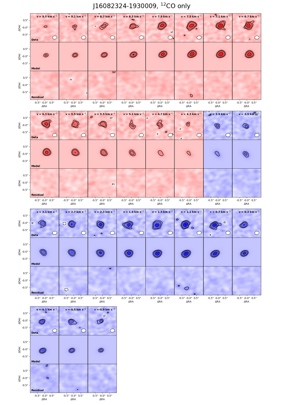
Figure 12: Channel maps showing the data, model, and residual for each channel over which the fit was performed. Panels in blue show emission that is blueshifted relative to V_LSR, and panels in red show redshifted emission. Each set of eight panels shows the data in the top row, the model in the middle row, and residuals in the bottom row. Velocity increases from left to right within each set of panels, and from top to bottom between panel sets. Contour levels are [3,5,10,15]$\times$rms, where rms is the median rms of the data cube. The complete figure set (29 items) is available in the online journal.

In Figure 13, we show an example of the full set of steps plots (parameter value versus step number for all walkers, for all parameters) for J16082324-1930009. The “lost” walkers are shown in gray. Channel maps and steps plots for all source$+$line combinations are available in the online material.

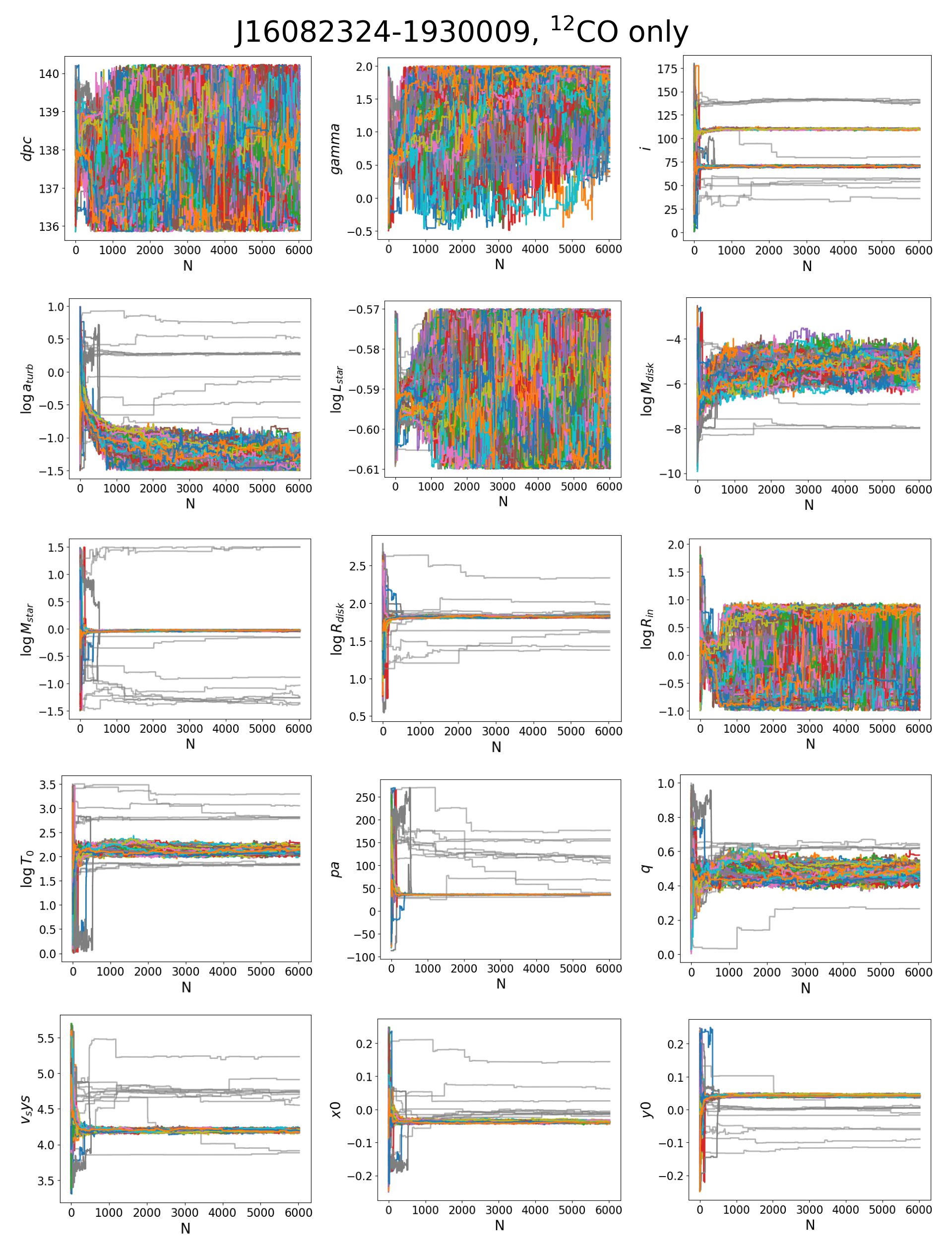
Figure 13: Steps plots (parameter value versus step number) for all 15 free parameters for target J16082324-1930009. The walkers meeting our $\chi^{2}$ cutoff are shown with colored lines, and the “lost” walkers are shown in gray. The complete figure set (29 items) is available in the online journal.

Appendix B Notes on Individual Sources

Some sources in the sample required special handling during the fitting process, returned stellar masses that are strongly inconsistent with the current literature, or could not be fit at all. We discuss each of these cases in greater detail below.

B.1 J15562477-2225552

Source J15562477-2225552 returned a distribution of M_⋆ that is clearly clustering toward the minimum of the parameter range (0.03 M_⊙). This is likely due to the low signal-to-noise of this source (5.8$\sigma$, the second-lowest in the sample) combined with its nearly face-on inclination (160${}^{+20}_{-20}$), which limits the emission to a narrow (projected) velocity range. For this source, we report the mass as an upper limit: M_⋆ $\leq$ 1.45M_⊙. This value corresponds to the 99.73% (3$\sigma$) probability in the Cumulative Distribution Function (CDF) of walker values from the previous 1000 steps.

B.2 J16035767-2031055 and J16142029-1906481

The fits for both J16035767-2031055 and J16142029-1906481 returned stellar masses that were notably inconsistent with the isochronal masses derived in this work, and with the masses and spectral types listed in Barenfeld et al. (2016). Those authors list a stellar mass of 1.0$\pm$0.1 M_⊙ and a spectral type of K5 for J16035767-2031055, and a stellar mass of 0.56${}^{+0.05}_{-0.06}$ and spectral type of M0 for J16142029-1906481. Our Keplerian modeling instead returns stellar masses of 4.0${}^{+4.0}_{-2.0}$ M_⊙ and 1.32${}^{+0.06}_{-0.06}$ M_⊙, respectively. These high masses persisted even when the fits were repeated with various modifications to the parameter ranges. We could not find any evidence of known or candidate companions for either source in the literature. Neither source is strongly edge-on ($i$ $\sim$ 90^∘), so they are unlikely to be “dipper” stars, and we were likewise unable to find clear evidence of variability in the literature.

The most likely explanation for these sources is that the exponentially-tapered flared disk model is not capturing some additional phenomenon traced in the CO data, such as disk winds and/or outflows. Both sources are unresolved in the continuum in our data, so we can neither confirm nor reject this possibility based on (mis)alignment between the CO and continuum major axes.

We could find no indications of (sub)millimeter-detected winds or outflows in the literature, but there is some useful information from shorter wavelengths. Fang et al. (2023) analyze high-resolution [OI] $\lambda$6300 and H$\alpha$ spectra from the Keck/HIRES archive for 115 T Tauri stars in Upper Sco, including both sources under consideration here. Relative to most of our sample, Fang et al. (2023) find that J16035767-2031055 has a comparatively bright low-velocity disk-wind component (log(L_BC/L_⊙)$=-$4.91, FWHM $=$ 42.3 km s^-1), and that J16142029-1906481 has both a bright high-velocity outflow component (log(L_HVC/L_⊙)$=-$4.19, FWHM $=$ 101.9 km s^-1) and a bright low-velocity wind component (log(L_SCJ/L_⊙)$=-$5.08, FWHM $=$ 31.6 km s^-1). Both sources are also resolved in CO, as shown in Figure 2. However, most sources in our sample have a low-velocity disk-wind component detected in [OI] $\lambda$6300 (typical log(L_LVC/L_⊙): $-$6.6 to $-$5.4 for our sources), and some have high-velocity components as well. Consequently, it is not clear whether the comparative brightness of these components in J16035767-2031055 and J16142029-1906481 could be solely responsible for the high dynamical masses we derive.

B.3 J16075796-2040087

Source J16075796-2040087 required an unusually long burn-in period ($\sim$4500 steps) due to large groups of “lost” walkers, i.e., walkers clumped in parameter space that did not survive our $\chi^{2}$ cut. Even after the fit achieved convergence, some parameters still had distinct bimodal distributions of walkers, and the walkers are clustered at the top edge of the allowed parameter range for $\gamma$. We suspect that, like the previous two sources, J16075796-2040087 exhibits emission that is not fully captured in our flared disk model.

J16075796-2040087 has a candidate companion identified in Barenfeld et al. (2019). The small projected separation between sources (6.3 au, well within their observed 1.3 mm disk radius), previous observations suggesting an accretion-powered outflow (Kraus & Hillenbrand, 2009), and observed periodic bursting behavior in the optical (Cody et al., 2017) led those authors to suggest that this source contains a circumbinary disk. It also has bright low-velocity (disk-wind) and high-velocity (collimated outflow) components in the [OI] $\lambda$6300 data of Fang et al. (2023). The observed outflows and bursting behavior could both potentially be contaminating the pdspy fit, if those processes are significantly impacting the CO emission. This source is also resolved in our CO data (see Figure 2); it is possible that internal disk structures are contributing to the issues present in this fit.

B.4 J16113134-1838259 B

Field J16113134-1838259 (also known as AS 205) contains two disks as well as significant large-scale, extended emission near V_LSR in our data. Some of this large-scale emission takes the form of an apparent gas bridge between the two sources. Both disks appear to be slightly warped, and non-Keplerian rotation has been observed in the northern source, J16113134-1838259 A (Kurtovic et al., 2018). Though this extended emission does not appear to suffer from spatial filtering in our data, it and the presence of two sources made J16113134-1838259 B (also known as AS 205 S) impossible to fit in ¹²CO. However, we did successfully fit its ¹³CO emission.

Source B is compact and moderately inclined ($\sim$65^∘). Consequently, is exhibits line emission over a much wider velocity range than either source A or the extended emission. We restricted the source position to $\Delta$RA, $\Delta$Dec $=$ $\pm$0$\farcs$15 as opposed to the standard $\pm$0$\farcs$25. This stricter position range prevented the walkers from erroneously including emission from source A. We also flagged out the channels covering V_LSR $\pm$2.2 km s^-1 in the MS file. The channel flagging ensures that the channels with the strongest emission from source A, and the strongest extended emission, are excluded from the fit. Again, this prevented the walkers from erroneously fitting to emission from source A and the extended emission. Because the line emission from source B spans V_LSR $\pm$ 5.4 km s^-1 and we assume Keplerian rotation at all radii, the exclusion of the central channels did not strongly impact the pdspy fit results. Source B was fit in 2520 steps with a standard burn-in interval of 1000 steps.

As for the field as a whole, Salyk et al. (2014) observed J16113134-1838259 in the then-highest spatial resolution (88 au at their assumed distance of 125 pc) in ALMA Cycle 0 with ¹²CO, ¹³CO, and C¹⁸O J$=$2$-$1 line emission and 232 GHz continuum emisison. They exclude molecular cloud emission, envelope emission, and accretion from a circumbinary disk as potential explanations for the extended emission and the non-Keplerian rotation observed in source J16113134-1838259 A (AS 205 N in their paper). They favor a low-velocity disk wind from J16113134-1838259 A as the most likely explanation for the observed emission, but note that they cannot exclude the possibility of tidal stripping of the source A disk by source B. Kurtovic et al. (2018), re-observed this source with 5 au resolution as part of the Disk Substructures at High Angular Resolutions Project (DSHARP, Andrews et al., 2018). These authors favor a flyby interaction as the explanation for the gas bridge between the disks, the large-scale arc-like structures, and the observed disk warping. However, both teams note the importance of accurate stellar masses - especially for source B - in constraining the parameters of a potential flyby interaction.

A detailed kinematic and modeling analysis of the full J16113134-1838259 system is beyond the scope of this paper. However, we call attention to the fact that our dynamically-derived results for this source (M_⋆ $=$ 1.53${}^{+0.14}_{-0.12}$ M_⊙) are higher than the previous best-estimate mass (M_⋆ $=$ 1.3 M_⊙) of Eisner et al. (2005) based on measurement uncertainties. This increase in mass ($\sim$18%) is consistent with the typical difference between our dynamical results and the isochronal methods. This increased, well-constrained mass will help place tighter constraints on the parameters of a potential flyby interaction in this field.

B.5 J16154416-1921171

Source J16154416-1921171 has strong ($\geq$6.5$\sigma$) emission in both ¹²CO and ¹³CO. However, it also has significant, large angular-scale line emission. This emission is partially resolved-out at V_LSR in both isotopologues. This spatial filtering made the source impossible to fit, even with channel and (u,v)-range flagging. It is therefore excluded from our results and analysis.

Appendix C Full Sample versus Mass-limited Sample

Table 7 showed statistics for both the full sample and the mass-limited sample. In § 5.2, we examined sample statistics and figures for only those sources with M_⋆ $\leq$ 1 M_⊙, which is the mass range common to all PMS model sets. Here, we show additional figures using the full sample and briefly discuss the impact of using the full sample on the statistics in Table 7.

In Figure 14, we show an alternate version of Figure 8 in which the x-axis extends up to 4.2 M_⊙. We show the best-fit lines for both the full-sample and mass-limited sample. The impact of the M_⋆ $\geq$ 1 M_⊙ sources, and in particular the source with M_dyn = 4.0 M_⊙, on the best-fit line can be clearly seen. Although none of the PMS model sets agree with the 1:1 line within uncertainties when the full sample is considered, the masses derived using the magnetic models of Feiden (2016) are still the least discrepant out of all model sets.

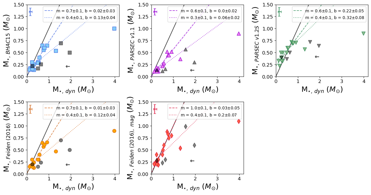
Figure 14: As for Figure 8, but showing the full range of dynamical masses for our data. The best-fit line for the full sample is shown as a dotted colored line in each panel, and the best fit for the mass-limited sample is shown as a dashed colored line. As in Figure 8, known or candidate binaries are shown with gray symbols, and the 1:1 relation is shown as a black solid line. Although no PMS model sets show a 1:1 relationship with dynamical mass when using the full sample, the mass values for Feiden (2016) magnetic models are still the least discrepant.

Figure 15 shows the Cumulative Distribution Functions (CDFs) of the isochronal masses and our dynamical masses using the full sample. Although the CDFs of the isochronal masses are not significantly impacted by including the M_dyn $>$ 1 M_⊙ sources (compare to Figure 9), the CDF for the dynamical masses clearly is. However, as demonstrated in Table 7, the impact of this inclusion on the KS test statistics is not large: $D$ changes by $\leq$0.1, with only nominal changes in corresponding p-values. No model sets are rejected with $\geq$4$\sigma$ confidence. The magnetic models of Feiden (2016) are still clearly the most similar to the dynamical masses ($D$ $=$ 0.18) compared to the other four model sets ($D$ $\geq$ 0.32).

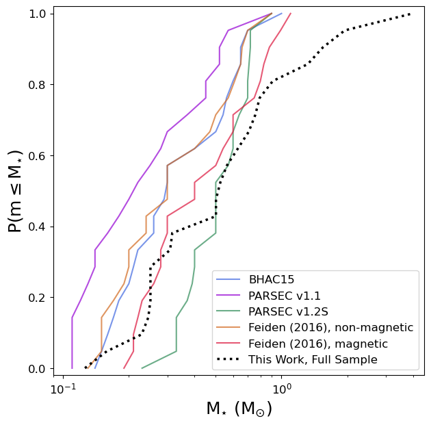
Figure 15: As for Figure 9, but showing the full range of dynamical masses for our data. The Cumulative Distribution Function (CDF) using our full sample is shown as a black dotted line. Compare to Figure 9.

Finally, for the remaining statistics listed in Table 7, excluding sources with M_⋆ $>$ 1 M_⊙ primarily impacts the mass ratios. The mass ratio minima decrease by $\sim$23-69% when the full sample is used. This is to be expected, as the most massive sources often show the greatest discrepancies between dynamical and isochronal mass. The mass ratio maxima are unchanged, and the median and mean mass ratios are unchanged within uncertainties. The PARSEC v1.2S median and mean ratios still have the largest uncertainties out of all the model sets, and the magnetic Feiden (2016) mean and mean mass ratios are both still with $\leq$10% of unity. The Spearman $\rho$ correlation coefficients become more negative in all cases, which is expected considering the positions of the excluded sources on the plots in Figure 14. The p-values of the coefficients all decrease by $>$2 orders of magnitude. However, the p-values for the BHAC15, PARSEC v1.1, and both Feiden (2016) models all remain $<$4$\sigma$, i.e. they still do not meet our threshold for statistical significance. The p-value for the PARSEC v1.2S models decreases to 4$\times$10^-9, and remains at $\geq$4$\sigma$ significance.

Taken together, these changes do not meaningfully alter our interpretations. We still conclude that the magnetic models of Feiden (2016) are more consistent with our dynamical masses than the other four model sets tested. We likewise still conclude that only the PARSEC v1.2S models show a statistically-significant correlation between mass and mass ratio (i.e. potential that the accuracy of the model set is mass-dependent). In short, we find that our results are robust against the inclusion or exclusion of sources with M_⋆ $>$ 1 M_⊙ from our sample.

Appendix D Impacts of Binarity and Methodology on the Observed Trends

D.1 Confirmed or Candidate Companions

The presence of binary or other close companions has the potential to impact the dynamical fitting results. In the case of bound companions outside the disk, the companion star has the potential distort the disk, depending on the companion’s current distance and/or any recent flyby encounters (e.g. Kurtovic et al., 2018). In the case of a circumbinary disk, the dynamical mass may be more discrepant with the isochronal mass if the companion is dim and undetected; likewise, circumbinary disks are also both theorized and observed to exhibit truncation, spirals, larger inner cavities and accretion rates than in single systems, and disk misalignment (Rosotti & Clarke, 2018; Penzlin et al., 2024; Cuello et al., 2025). In both cases, the comparison between isochronal and dynamical results could be strongly affected.

Five targets in our sample have confirmed or candidate companions: J15534211$-$2114135, J16001844$-$2230114, J16014086$-$2258103, J16075796$-$2040087, and J16113134-183259 B. Bouy et al. (2006) detect a companion for J16014086$-$2258103 in $Ks$-band (2.18 $\mu$m) using the Nasmyth Adaptive Optics System Near-Infrared Imager and Spectrograph (NACO; Rousset et al., 2003; Lenzen et al., 2003) on the Very Large Telescope (VLT). The separation between this source and its companion put the companion outside the disk radius, at a projected linear separation of 706$\pm$1 mas ($\sim$ 88 au based on the Gaia distance). Barenfeld et al. (2019) search for candidate companions for 113 G2$-$M5 stars in Upper Sco, including all targets in our sample. They use the Near-Infrared Camera (NIRC2; instrument PI: Keith Matthews) on the Keck II telescope to obtain both AO and aperture-masked $K$-band (2.196 $\mu$m) images for their targets. Barenfeld et al. (2019) find new candidate companions for J15534211$-$2114135, J16001844$-$2230114, and J16075796$-$2040087. In all three cases, the candidate companion lies within the radius of the continuum disk. J15534211$-$2114135 has two candidate companions: one at a projected linear separation of 321.8$\pm$1 mas ($\sim$11.5 au at the distance to this source), and the other at 1097.1$\pm$0.1 mas ($\sim$38 au). The location of the more distant companion puts it well outside the observed disk radius. (Eisner et al., 2005) observe source J16113134-183259 B (designated AS205B in that work) using the Keck I High-Resolution Echelle Spectrometer (HIRES, Vogt et al., 1994). They classify this source as a spectroscopic binary.

To investigate whether binary systems may be skewing our results, we re-calculate all statistics excluding these five sources. We find that the majority of our results do not change. The main exception is the relationship between source mass ratio and dynamical mass, which is moderately sensitive to the inclusion of the binary candidates. We describe the impact of binary exclusion on each statistical value below:

1. The mass ratios themselves exhibit three consistent changes: 1) no change or a slight increase in the minimum mass ratio (never a decrease), 2) a slight increase in the mean and median mass ratios, and 3) a slight decrease in the scaled MAD and standard deviation of the mass ratios. This is true regardless of whether we consider the full sample or only the mass-limited sample. The increases in minimum, median, and mean mass ratio are expected, because two of the three most massive sources in the sample (by M_dyn) are binaries. The corresponding decrease in scaled MAD and standard deviation are also consistent with this explanation. However, all changes are within the uncertainties of both the new and original values, i.e., there are no statistically-significant changes in mass ratio.

2. The Spearman $\rho$ coefficients for the full sample show the largest change. The coefficients themselves (Table 7, column 6) all remain negative, but their p-values (column 7) increase by an order of magnitude in all cases. This drops the p-values below a 3$\sigma$ significance level for all model sets except the PARSEC v1.2S models, which remain at $>$5$\sigma$ significance.

3. The Spearman $\rho$ coefficients for the mass-limited sample show almost no change. As with the mass ratios, this is consistent with the fact that two of the four most massive sources are binaries - applying a mass limit of M_⋆ $\leq$ 1 M_⊙ effectively removes them from the sample before binarity is even considered. The only exception is, again, the PARSEC v1.2S models, for which the p-value decreases from 1$\times$10^-5 to 3$\times$10^-6.

4. The KS test p-values increase in all cases. However, because all KS-test p-values were high to begin with, this does not change our interpretations. The D-values decrease slightly in all cases except for the PARSEC v1.2S models, for which the D-values increase slightly in both the full-sample and mass-limited cases. The smaller D-values are consistent with decreased scatter in our data. As Figure 15 shows, most of the deviation between the dynamical mass CDF and those of the isochronal masses comes at the high-mass end. Removing most of the highest-mass sources (50% of which are known binaries) brings our CDF into better alignment with all of the isochrones except for the PARSEC v1.2S models.

Overall, we find that excluding the binary sources from our sample has little impact on the sample statistics for either the full or the mass-limited sample case. Our interpretations and conclusions remain unchanged.

Finally, we find that excluding our known or candidate binary systems has no significant impact on the derived relationship between disk dust mass and stellar dynamical mass. For the assumption that dust temperature scales with L_⋆, the best-fit line has an initial slope of 2.8$\pm$0.6 and intercept of 1.0$\pm$0.3. After removing the binary systems, the best-fit line has a slope of 2.8$\pm$0.7 and intercept of 1.1$\pm$0.3, i.e. statistically identical but with a slight increase in uncertainty. Assuming a constant T_dust $=$ 20 K, our best-fit line using all sources has a slope of 2.8$\pm$0.5 and intercept of 0.9$\pm$0.2; removing the binary systems changes this to a slope of 2.8$\pm$0.6 and intercept of 0.9$\pm$0.3, i.e. again identical within uncertainties.

D.2 Disk Inclination, Stellar Mass, and the Keplerian-fitting Method

The inclination of a disk can have a strong impact on our ability to accurately model the stellar mass. For a star of any given mass $M$ and inclination $i$, the true Keplerian velocity at radius $r$ in the disk will be $v(r)_{true}$ $=$ $\sqrt{GM/r}$, but the corresponding observed velocity will be $v(r)_{obs}$ $=$ $(sin\,\,i)\sqrt{GM/r}$. As inclination decreases, the observed range of velocities $v_{max,\,obs}$ $-$ $v_{min,\,obs}$ will also decrease. This makes a disk of mass $M$ progressively more difficult to detect at lower inclinations, and is especially detrimental for lower-mass sources, whose maximum Keplerian velocities will be lower to begin with.

In principle, the pdspy modeling procedure should be agnostic to both stellar mass and inclination angle. The physics of the disk model itself, the specifics of the walker step selection, and the $\chi^{2}$ minimization routine neither assume nor require a particular stellar mass or inclination value. However, as a practical matter, the comparatively smaller velocity range observed for a low-inclination disk means that the model will have fewer data points to fit to overall. This could result in high uncertainties, an inability to distinguish between degenerate possibilities (e.g. a low-mass, high-inclination source and a high-inclination, low-mass source), or an inability to achieve a successful fit at all. This is an even more significant concern for small or low signal-to-noise disks, which will further narrow the range of ($u,v$) space over which pdspy can fit to the data.

Conversely, the high extinction caused by edge-on disks can bias inferred stellar spectral types in the opposite direction. High extinction will decrease the overall stellar luminosity, and will redden the observed colors of the star. Both factors can result in a later inferred spectral type than is actually true, and can potentially bias the spectral-type analysis toward lower masses and/or higher ages.

We have examined whether there is any trend in stellar mass with derived inclination angle for our sample. We compare stellar mass versus inclination for our Upper Sco sources to the trends detailed in Barenfeld et al. (2017), which examines a sample of 55 continuum-detected disks in Upper Sco that includes all sources in our sample. These authors use the stellar masses of Barenfeld et al. (2016), and derive inclination angle(s) for each disk using dust-continuum emission (55 disks) and, where possible, ¹²CO emission (23 disks). Figure 16 shows mass versus inclination for our data compared to both the continuum- and CO-derived inclinations from Barenfeld et al. (2017).

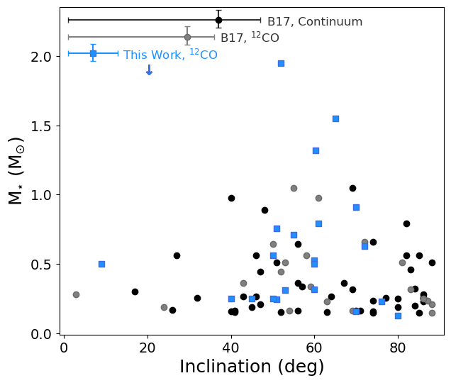
Figure 16: Stellar mass versus inclination angle for the CO-derived M_⋆ and $i$ in this work (blue), the CO-derived M_⋆ and $i$ in Barenfeld et al. (2017) (grey), and the continuum-derived M_⋆ and $i$ in Barenfeld et al. (2017) (black). We find that our derived masses and inclination angles show no bias compared to the Barenfeld et al. (2017) data, but that all samples suffer from small-number statistics at the lower ($<$30^∘) and highest ($>$85^∘) inclinations.

The three samples appear to occupy the same parameter space in M_⋆ versus $i$ in Figure 16. To quantify the similarity between samples, we calculate Spearman $\rho$ coefficients and p-values between $i$ and M_⋆ for all three data sets. The data obtained from line emission (our data and the Barenfeld et al. (2017) CO data) have slight negative correlations between mass and inclination angle, but the correlation does not rise above 2$\sigma$ in either case (p $=$ 0.68 and 0.25, respectively). The mass$-$inclination data obtained from the continuum observations have a slight positive correlation, but the p-value again indicates no statistical significance (p $=$ 0.9). We additionally examine the median and scaled MAD of M_⋆ and $i$ for each of the three data sets. We find that the medians agree within uncertainties for both properties for all three data sets ($i$ $=$ 58$\pm$11, 60$\pm$16, 68$\pm$24, and M_⋆ $=$ 0.5$\pm$0.4, 0.3$\pm$0.2, 0.3$\pm$0.1). Finally, we perform a KS-test analysis for $i$ and M_⋆ separately, and compare each data set to the other two. We find that no KS-test p-values are consistent with a $\geq$4$\sigma$ significance (p-values ranged from 0.04 to 0.8), indicating that the three data sets are not significantly different in either $i$ or M_⋆. We conclude from these results that our method of deriving stellar mass $-$ Keplerian fitting using the pdspy package $-$ has not introduced a bias in derived mass with inclination angle.

Appendix E Description of the Pre-Main Sequence Evolutionary Models

The five stellar evolutionary models we evaluate in this work represent three of the most widely-used schools of models applicable to low-mass stars: the Baraffe models (BHAC15), the Padova stellar evolution code (PARSEC v1.1 and 1.2S), and the Dartmouth models (Feiden, 2016).

E.1 BHAC15

The BHAC15 stellar evolutionary models (Baraffe et al., 2015) are a set of models developed primarily for low-mass stars, and cover the mass range 0.01-1.4 M_⊙. They are an update to the widely-used BCAH98 models (Baraffe et al., 1998), which cover 0.075-1.0 M_⊙. Both BCAH98 and BHAC15 model the structure and evolution of stellar interiors following the physics of Chabrier & Baraffe (1997). The most significant change in BHAC15 is a replacement of the NextGen stellar atmospheric models (Hauschildt et al., 1999) with the BT-Settl atmospheric models (Allard et al., 2012). Additionally, BHAC15 includes an expanded molecular linelist compared to BCAH98, which used only solar-type metallicities. The revised models of Baraffe et al. (2015) solve the known issue of BCAH98 predicting optical colors (V-I) that were too blue for a given magnitude.

E.2 PARSEC v1.1

The PAdova and TRieste Stellar Evolution Code (PARSEC, Bressan et al., 2012) is a revision and expansion of the Padova stellar evolution code (Bressan et al., 1993). Most notably, the PARSEC models expand Padova to include the pre-main sequence (PMS) phase of stellar evolution, using the physics and boundary conditions described below. They span a mass range of M_⋆ $=$ 0.1-12 M_⊙ and a metallicity range of $Z$ $=$ 0.0005 to 0.07. The PARSEC models calculate the equation of state using the FreeEOS library in FORTRAN (Alan W. Irwin, copyright 2008 under GPL license, https://freeeos.sourceforge.net/). They implement a temperature gradient described by the mixing-length theory of Böhm-Vitense (1958), include a revised nuclear network and reaction rates (Cyburt et al., 2010), and add microscopic diffusion to the model physics. They also implement an opacity-table generation tool that allows the user to create models for any initial chemical composition using opacities from AESOPUS (Marigo & Aringer, 2009) and OPAL (Iglesias & Rogers, 1996). As the PARSEC code later underwent several revisions, this original version is referred to as PARSEC v1.1.

E.3 PARSEC v1.2S

The PARSEC v1.2S (Chen et al., 2014) models are an update to the PARSEC v1.1 code of Bressan et al. (2012), described above. The v1.2S models aim to address known issues with modeling low-mass stars specifically ($\leq$0.6 M_⊙). In particular, the PARSEC v1.1 models show a consistent discrepancy between observed and model radii, which leads to a $\sim$8% discrepancy in the mass-radius relation in the models. They also tend to produce too-blue optical colors for low-mass main-sequence stars. PARSEC v1.2S applies the $T-\tau$ relation of the BT-Settl atmospheric models as an outer boundary condition in the PARSEC code. This change reduces the mass-radius discrepancy to 5%. It also reduces, though does not eliminate, the discrepancies in the optical colors.

E.4 Feiden (2016) standard and magnetic models

Feiden (2016) seeks to address the known tendency of PMS stellar evolutionary models of late-type (K, M) stars to return much younger ages than for more massive stars (A, F, G) in the same group or cluster. The underlying premise of the Feiden (2016) magnetic models is that magnetic fields in these cool dwarfs inhibit convection, which slows the star’s contraction and thus extends the amount of time they spend on the Hayashi track. The result is that the age inferred from a given mass, radius, and isochrone will be too low for these late-type stars, if the stellar evolutionary model used does not account for this magnetic inhibition.

The magnetic models of Feiden (2016) are based on the magnetic Dartmouth stellar evolution models of Feiden & Chaboyer (2012). Those models are, in turn, based on the original standard models produced by the Dartmouth Stellar Evolution Program (DSEP, Dotter et al., 2008). In addition to magnetic fields, the Feiden (2016) models incorporate model atmosphere structures generated using a custom grid that combines the solar composition of Grevesse & Sauval (1998) with the opacities of Ferguson et al. (2005) for low temperatures. The models also include explicit treatment of deuterium burning, and the implementation of a boundary condition at the $\tau_{5000}$ $=$ 10 surface.

In the Feiden (2016) models, the magnetic field strength is Gaussian with radius, centered at the location of the inner boundary of the stars’ convective layer. The interaction between the magnetic field, convection, and the plasma equation of state follow the physics described in Feiden & Chaboyer (2012, 2013). The model assumes equipartition between the gas pressure and the magnetic field pressure at the star’s surface, with typical surface magnetic field strengths of 2.5 kG (corresponding to typical peak magnetic field strengths of 50 kG in the star’s interior). The magnetic field is “switched on” at a stellar age of 0.1 to 0.5 Myr. It is switched off if and when the star’s outer convective envelope disappears, which occurs only for M_⋆ $\gtrsim$ 1.15 M_⊙.

References

- Allard et al. (2011) Allard, F., Homeier, D., & Freytag, B. 2011, 16th Cambridge Workshop on Cool Stars, Stellar Systems, and the Sun, 448, 91
- Allard et al. (2012) Allard, F., Homeier, D., & Freytag, B. 2012, Philosophical Transactions of the Royal Society of London Series A, 370, 2765
- Allen (1973) Allen, C. W. 1973, London: University of London, Athlone Press, —c1973, 3rd ed.
- Andrews et al. (2013) Andrews, S. M., Rosenfeld, K. A., Kraus, A. L., et al. 2013, ApJ, 771, 129
- Andrews et al. (2018) Andrews, S. M., Huang, J., Pérez, L. M., et al. 2018, ApJ, 869, L41
- Astropy Collaboration et al. (2013) Astropy Collaboration, Robitaille, T. P., Tollerud, E. J., et al. 2013, A&A, 558, A33
- Astropy Collaboration et al. (2018) Astropy Collaboration, Price-Whelan, A. M., Sipőcz, B. M., et al. 2018, AJ, 156, 123
- Astropy Collaboration et al. (2022) Astropy Collaboration, Price-Whelan, A. M., Lim, P. L., et al. 2022, ApJ, 935, 167
- Baraffe et al. (1998) Baraffe, I., Chabrier, G., Allard, F., et al. 1998, A&A, 337, 403
- Baraffe et al. (2015) Baraffe, I., Homeier, D., Allard, F., et al. 2015, A&A, 577, A42
- Barenfeld et al. (2016) Barenfeld, S. A., Carpenter, J. M., Ricci, L., et al. 2016, ApJ, 827, 142
- Barenfeld et al. (2017) Barenfeld, S. A., Carpenter, J. M., Sargent, A. I., et al. 2017, ApJ, 851, 85
- Barenfeld et al. (2019) Barenfeld, S. A., Carpenter, J. M., Sargent, A. I., et al. 2019, ApJ, 878, 45
- Bary & Petersen (2014) Bary, J. S. & Petersen, M. S. 2014, ApJ, 792, 64
- Bell et al. (2012) Bell, C. P. M., Naylor, T., Mayne, N. J., et al. 2012, MNRAS, 424, 3178
- Bergin et al. (2024) Bergin, E. A., Bosman, A., Teague, R., et al. 2024, ApJ, 965, 147
- Blaauw (1946) Blaauw, A. 1946, Publications of the Kapteyn Astronomical Laboratory Groningen, 52, 1
- Blaauw (1964) Blaauw, A. 1964, ARA&A, 2, 213
- Böhm-Vitense (1958) Böhm-Vitense, E. 1958, ZAp, 46, 108
- Bouy et al. (2006) Bouy, H., Martín, E. L., Brandner, W., et al. 2006, A&A, 451, 177
- Braun et al. (2021) Braun, T. A. M., Yen, H.-W., Koch, P. M., et al. 2021, ApJ, 908, 46
- Bressan et al. (1993) Bressan, A., Fagotto, F., Bertelli, G., et al. 1993, A&AS, 100, 647
- Bressan et al. (2012) Bressan, A., Marigo, P., Girardi, L., et al. 2012, MNRAS, 427, 127
- Cardelli et al. (1989) Cardelli, J. A., Clayton, G. C., & Mathis, J. S. 1989, ApJ, The Relationship between Infrared, Optical, and Ultraviolet Extinction, 345, 245.
- Carpenter et al. (2025) Carpenter, J. M., Esplin, T. L., Luhman, K. L., et al. 2025, ApJ, 978, 117
- CASA Team et al. (2022) CASA Team, Bean, B., Bhatnagar, S., et al. 2022, PASP, 134, 114501
- Chabrier & Baraffe (1997) Chabrier, G. & Baraffe, I. 1997, A&A, 327, 1039
- Chen et al. (2014) Chen, Y., Girardi, L., Bressan, A., et al. 2014, MNRAS, 444, 2525
- Cody et al. (2017) Cody, A. M., Hillenbrand, L. A., David, T. J., et al. 2017, ApJ, 836, 41
- Cohen & Kuhi (1979) Cohen, M. & Kuhi, L. V. 1979, ApJS, 41, 743
- Comrie et al. (2021) Comrie, A., Wang, K.-S., Hsu, S.-C., et al. 2021, Zenodo
- Cuello et al. (2025) Cuello, N., Alaguero, A., & Poblete, P. P. 2025, arXiv:2501.19249
- Cyburt et al. (2010) Cyburt, R. H., Amthor, A. M., Ferguson, R., et al. 2010, ApJS, 189, 240
- Czekala et al. (2015) Czekala, I., Andrews, S. M., Jensen, E. L. N., et al. 2015, ApJ, 806, 154
- David et al. (2019) David, T. J., Hillenbrand, L. A., Gillen, E., et al. 2019, ApJ, 872, 161
- DENIS Consortium (2005) DENIS Consortium 2005, VizieR Online Data Catalog, VizieR Online Data Catalog: The DENIS database (DENIS Consortium, 2005), 1. B/denis
- Dickman (1978) Dickman, R. L. 1978, ApJS, 37, 407
- Dotter et al. (2008) Dotter, A., Chaboyer, B., Jevremović, D., et al. 2008, ApJS, 178, 89
- Dullemond et al. (2012) Dullemond, C. P., Juhasz, A., Pohl, A., et al. 2012, Astrophysics Source Code Library
- Eisner et al. (2005) Eisner, J. A., Hillenbrand, L. A., White, R. J., et al. 2005, ApJ, 623, 952
- Encrenaz et al. (1975) Encrenaz, P. J., Falgarone, E., & Lucas, R. 1975, A&A, 44, 73
- Fang et al. (2023) Fang, M., Pascucci, I., Edwards, S., et al. 2023, ApJ, 945, 112
- Feiden & Chaboyer (2012) Feiden, G. A. & Chaboyer, B. 2012, ApJ, 761, 30
- Feiden & Chaboyer (2013) Feiden, G. A. & Chaboyer, B. 2013, ApJ, 779, 183
- Feiden (2016) Feiden, G. A. 2016, A&A, 593, A99
- Ferguson et al. (2005) Ferguson, J. W., Alexander, D. R., Allard, F., et al. 2005, ApJ, 623, 585
- Flores et al. (2022) Flores, C., Connelley, M. S., Reipurth, B., et al. 2022, ApJ, 925, 21
- Flewelling et al. (2020) Flewelling, H. A., Magnier, E. A., Chambers, K. C., et al. 2020, ApJS, 251, 1, 7
- Fouqué et al. (2000) Fouqué, P., Chevallier, L., Cohen, M., et al. 2000, A&AS, 141, 313
- Foreman-Mackey et al. (2013) Foreman-Mackey, D., Hogg, D. W., Lang, D., et al. 2013, PASP, 125, 306
- Frank et al. (2014) Frank, A., Ray, T. P., Cabrit, S., et al. 2014, Protostars and Planets VI, 451
- Gaia Collaboration et al. (2016) Gaia Collaboration, Prusti, T., de Bruijne, J. H. J., et al. 2016, A&A, 595, A1
- Gaia Collaboration et al. (2018) Gaia Collaboration, Brown, A. G. A., Vallenari, A., et al. 2018, A&A, 616, A1
- Gaia Collaboration et al. (2021) Gaia Collaboration, Brown, A. G. A., Vallenari, A., et al. 2021, A&A, 649, A1
- Gavras et al. (2023) Gavras, P., Rimoldini, L., Nienartowicz, K., et al. 2023, A&A, 674, A22
- Ginsburg et al. (2014) Ginsburg, A., Robitaille, T., Beaumont, C., & ZuHone, J. (2014). Release Candidate 2 - includes yt interop (v0.2-rc2). Zenodo. https://doi.org/10.5281/zenodo.11485
- Girardi et al. (2002) Girardi, L., Bertelli, G., Bressan, A., et al. 2002, A&A, 391, 195
- Grevesse & Sauval (1998) Grevesse, N. & Sauval, A. J. 1998, Space Sci. Rev., 85, 161
- Hauschildt et al. (1999) Hauschildt, P. H., Allard, F., & Baron, E. 1999, ApJ, 512, 377
- Haworth et al. (2018) Haworth, T. J., Booth, R. A., Homan, W., et al. 2018, MNRAS, 473, 317
- Henden & Munari (2014) Henden, A. & Munari, U. 2014, Contributions of the Astronomical Observatory Skalnaté Pleso, 43, 3, 518
- Henden et al. (2018) Henden, A. A., Levine, S., Terrell, D., et al. 2018, \aas, 232, 223.06
- Henden (2019) Henden, A. A. 2019, \jaavso, 47, 1, 130
- Herczeg & Hillenbrand (2015) Herczeg, G. J. & Hillenbrand, L. A. 2015, ApJ, 808, 23
- Hillenbrand & White (2004) Hillenbrand, L. A. & White, R. J. 2004, ApJ, 604, 741
- Iglesias & Rogers (1996) Iglesias, C. A. & Rogers, F. J. 1996, ApJ, 464, 943
- Kraus et al. (2008) Kraus, A. L., Ireland, M. J., Martinache, F., et al. 2008, ApJ, 679, 762
- Kraus & Hillenbrand (2009) Kraus, A. L. & Hillenbrand, L. A. 2009, ApJ, 703, 1511
- Kurtovic et al. (2018) Kurtovic, N. T., Pérez, L. M., Benisty, M., et al. 2018, ApJ, 869, L44
- Lenzen et al. (2003) Lenzen, R., Hartung, M., Brandner, W., et al. 2003, Proc. SPIE, 4841, 944
- Luhman (1999) Luhman, K. L. 1999, ApJ, Young Low-Mass Stars and Brown Dwarfs in IC 348, 525, 1, 466
- Luhman & Mamajek (2012) Luhman, K. L. & Mamajek, E. E. 2012, ApJ, The Disk Population of the Upper Scorpius Association, 758, 1, 31
- Luhman & Esplin (2020) Luhman, K. L. & Esplin, T. L. 2020, AJ, 160, 44
- Luhman (2022a) Luhman, K. L. 2022, AJ, 163, 24
- Lynden-Bell & Pringle (1974) Lynden-Bell, D. & Pringle, J. E. 1974, MNRAS, 168, 603
- Magnier et al. (2020) Magnier, E. A., Schlafly, E. F., Finkbeiner, D. P., et al. 2020, ApJS, 251, 1, 6
- Manara et al. (2023) Manara, C. F., Ansdell, M., Rosotti, G. P., et al. 2023, Protostars and Planets VII, 534, 539
- Marigo & Aringer (2009) Marigo, P. & Aringer, B. 2009, A&A, 508, 1539
- Marigo et al. (2017) Marigo, P., Girardi, L., Bressan, A., et al. 2017, ApJ, 835, 77
- Marton et al. (2023) Marton, G., Ábrahám, P., Rimoldini, L., et al. 2023, A&A, 674, A21
- McMullin et al. (2007) McMullin, J. P., Waters, B., Schiebel, D., et al. 2007, Astronomical Data Analysis Software and Systems XVI, 376, 127
- Miret-Roig et al. (2022) Miret-Roig, N., Galli, P. A. B., Olivares, J., et al. 2022, A&A, 667, A163
- Munari et al. (2014) Munari, U., Henden, A., Frigo, A., et al. 2014, AJ, 148, 5, 81
- Palla & Stahler (1993) Palla, F. & Stahler, S. W. 1993, ApJ, 418, 414
- Pascucci et al. (2016) Pascucci, I., Testi, L., Herczeg, G. J., et al. 2016, ApJ, 831, 125
- Pecaut et al. (2012) Pecaut, M. J., Mamajek, E. E., & Bubar, E. J. 2012, ApJ, 746, 154
- Pecaut & Mamajek (2013) Pecaut, M. J. & Mamajek, E. E. 2013, ApJS, Intrinsic Colors, Temperatures, and Bolometric Corrections of Pre-main-sequence Stars, 208, 1, 9
- Pegues et al. (2021) Pegues, J., Czekala, I., Andrews, S. M., et al. 2021, ApJ, 908, 42
- Penzlin et al. (2024) Penzlin, A. B. T., Booth, R. A., Nelson, R. P., et al. 2024, MNRAS, 532, 3166
- Pérez Paolino et al. (2024) Pérez Paolino, F., Bary, J. S., Hillenbrand, L. A., et al. 2024, ApJ, 967, 45
- Piétu et al. (2007) Piétu, V., Dutrey, A., & Guilloteau, S. 2007, A&A, 467, 163
- Preibisch et al. (2002) Preibisch, T., Brown, A. G. A., Bridges, T., et al. 2002, AJ, 124, 404
- Preibisch & Mamajek (2008) Preibisch, T. & Mamajek, E. 2008, Handbook of Star Forming Regions, Volume II, 235
- Press et al. (1992) Press, W. H., Teukolsky, S. A., Vetterling, W. T., et al. 1992, Cambridge: University Press, —c1992, 2nd ed.
- Ratzenböck et al. (2023a) Ratzenböck, S., Großschedl, J. E., Möller, T., et al. 2023, A&A, 677, A59
- Ratzenböck et al. (2023b) Ratzenböck, S., Großschedl, J. E., Alves, J., et al. 2023, A&A, 678, A71
- Rimoldini et al. (2023) Rimoldini, L., Holl, B., Gavras, P., et al. 2023, A&A, 674, A14
- Rizzuto et al. (2016) Rizzuto, A. C., Ireland, M. J., Dupuy, T. J., et al. 2016, ApJ, 817, 164
- Rosotti & Clarke (2018) Rosotti, G. P. & Clarke, C. J. 2018, MNRAS, 473, 5630
- Rousset et al. (2003) Rousset, G., Lacombe, F., Puget, P., et al. 2003, Proc. SPIE, 4839, 140
- Roy (2020) Roy, V. 2020, Annual Review of Statistics and Its Application, 7, 387
- Rydgren & Vrba (1983) Rydgren, A. E. & Vrba, F. J. 1983, AJ, 88, 1017
- Salyk et al. (2014) Salyk, C., Pontoppidan, K., Corder, S., et al. 2014, ApJ, 792, 68
- Sanna et al. (2019) Sanna, A., Kölligan, A., Moscadelli, L., et al. 2019, A&A, 623, A77
- Sartori et al. (2003) Sartori, M. J., Lépine, J. R. D., & Dias, W. S. 2003, A&A, 404, 913
- Schmidt-Kaler (1982) Schmidt-Kaler, T. 1982, Bulletin d’Information du Centre de Donnees Stellaires, Automated spectral classification. A survey, 23, 2.
- Semenov et al. (2024) Semenov, D., Henning, T., Guilloteau, S., et al. 2024, A&A, 685, A126
- Sheehan (2018) Sheehan, P. 2018, Zenodo
- Sheehan et al. (2019) Sheehan, P. D., Wu, Y.-L., Eisner, J. A., et al. 2019, ApJ, 874, 136
- Skrutskie et al. (2006) Skrutskie, M. F., Cutri, R. M., Stiening, R., et al. 2006, AJ, The Two Micron All Sky Survey (2MASS), 131, 2, 1163
- Siess et al. (2000) Siess, L., Dufour, E., & Forestini, M. 2000, A&A, 358, 593
- Simon et al. (2019) Simon, M., Guilloteau, S., Beck, T. L., et al. 2019, ApJ, 884, 42
- Soderblom et al. (2014) Soderblom, D. R., Hillenbrand, L. A., Jeffries, R. D., et al. 2014, Protostars and Planets VI, 219
- Somers & Pinsonneault (2015) Somers, G. & Pinsonneault, M. H. 2015, ApJ, 807, 174
- Somers et al. (2020) Somers, G., Cao, L., & Pinsonneault, M. H. 2020, ApJ, 891, 29
- Straižys (1992) Straižys, V. 1992, , Multicolor stellar photometry.
- Steenman & The (1991) Steenman, H. & The, P. S. 1991, Ap&SS, The Anomalous Extinction Law - Part Two - the Effect of Changing the Lower Size Cutoff of the Particle Size Distribution, 184, 1, 9
- Tazzari et al. (2018) Tazzari, M., Beaujean, F., & Testi, L. 2018, MNRAS, 476, 4527
- Tonry et al. (2012) Tonry, J. L., Stubbs, C. W., Lykke, K. R., et al. 2012, ApJ, 750, 2, 99
- Vogt et al. (1994) Vogt, S. S., Allen, S. L., Bigelow, B. C., et al. 1994, Proc. SPIE, 2198, 362
- Wang & Chen (2019) Wang, S. & Chen, X. 2019, ApJ, 877, 2, 116
- Wenger et al. (2000) Wenger, M., Ochsenbein, F., Egret, D., et al. 2000, A&AS, The SIMBAD astronomical database. The CDS reference database for astronomical objects, 143, 9
- Yen et al. (2016) Yen, H.-W., Koch, P. M., Liu, H. B., et al. 2016, ApJ, 832, 204
- Yen et al. (2018) Yen, H.-W., Koch, P. M., Manara, C. F., et al. 2018, A&A, 616, A100
- Zacharias et al. (2013) Zacharias, N., Finch, C. T., Girard, T. M., et al. 2013, AJ, 145, 2, 44