Optimal estimation for regression discontinuity design
with binary outcomes.

Abstract

We develop a finite-sample optimal estimator for regression discontinuity designs when the outcomes are bounded, including binary outcomes as the leading case. Our finite-sample optimal estimator achieves the exact minimax mean squared error among linear shrinkage estimators with nonnegative weights when the regression function of a bounded outcome lies in a Lipschitz class. Although the original minimax problem involves an iterating ($n$+1)-dimensional non-convex optimization problem where $n$ is the sample size, we show that our estimator is obtained by solving a convex optimization problem. A key advantage of our estimator is that the Lipschitz constant is the only tuning parameter. We also propose a uniformly valid inference procedure without a large-sample approximation. In a simulation exercise for small samples, our estimator exhibits smaller mean squared errors and shorter confidence intervals than conventional large-sample techniques which may be unreliable when the effective sample size is small. We apply our method to an empirical multi-cutoff design where the sample size for each cutoff is small. In the application, our method yields informative confidence intervals, in contrast to the leading large-sample approach.

T1 The study was supported by JSPS KAKENHI Grant Numbers JP22K13373 (Ishihara), and JP21K13269 (Sawada). We thank Yu-Chang Chen, Atsushi Inoue, Timothy Neal, Michal Kolesár, Soonwoo Kwon and Ke-Li Xu, as well as seminar participants at Japanese Joint Statistical Meeting, Hitotsubashi University, Kansai Keiryo Keizaigaku Kenkyukai and Tohoku-NTU Joint Seminar, Econometric Society World Congress 2025 for insightful comments. T2First Version: October 6, 2025

1 Introduction

Large-sample approximation is the basis for the leading estimators for regression discontinuity (RD) designs (Imbens and Kalyanaraman, 2012; Calonico et al., 2014, for example). RD designs involve the estimation of conditional expectation functions at a cutoff point on the support of a running variable. Hence, the effective observations are limited to the neighborhood of the cutoff, and the number of these observations can be small even if the total sample size is large (Cattaneo et al., 2015; Canay and Kamat, 2017). For example, the effective sample can be small for designs with multiple cutoffs, with a cutoff at the tail of the distribution, or with subgroup analyses. In small samples, the large-sample asymptotics may not provide good approximations of the behaviors of the existing estimators, and hence, their stated desirable properties may be lost.

A few studies consider finite-sample minimax estimators for RD designs. For example, Armstrong and Kolesár (2018) and Imbens and Wager (2019) propose finite-sample minimax linear estimators under smoothness of the regression function. However, these minimax estimators require the knowledge of the conditional variance function, which is unknown in practice. While the variance can be estimated, we cannot guarantee the theoretical validity of the plug-in estimators with the estimated variance in finite samples. Furthermore, the construction of finite-sample valid confidence intervals based on these estimators additionally requires the normality of the regression errors.

In this study, we propose finite-sample estimation and inference methods for RD designs with binary outcomes. For a binary dependent variable, all features of its conditional distribution, including its conditional variance, are a known function of its conditional mean function. We establish the finite-sample validity of our methods under a smoothness restriction on the conditional mean function, taking into account the implicit restrictions it imposes on the entire conditional distribution. In other words, our procedure is both feasible and theoretically valid without either the knowledge or estimation of the conditional variance, or more generally, any features of the conditional distribution except the smoothness of the conditional mean.

More specifically, we consider a minimax optimal estimator among a class of linear shrinkage estimators for the regression function at a boundary point where the regression function satisfies the Lipschitz continuity. The class of linear shrinkage estimators is of the form $\sum_{i=1}^{n}w_{i}(Y_{i}-1/2)+1/2$ with $\sum_{i=1}^{n}w_{i}\leq 1$ and $w_{i}\geq 0$, where $Y_{1},...,Y_{n}$ are the observed outcomes on either side of the boundary. The shrinkage toward $1/2$ is motivated by the fact that the regression function is bounded and takes values in $[0,1]$, leading to a scope of efficiency gain by shrinkage. Given the class of linear shrinkage estimators, we derive a linear shrinkage estimator that minimizes the maximum mean squared error (MSE) under the Lipschitz continuity with a known Lipschitz constant. In other words, we assume the researcher’s a priori knowledge of the bound on how much the function value can change if the running variable is changed by one unit. We emphasize that this Lipschitz constant is the only tuning parameter. Furthermore, we show that the minimax estimator is the solution to a convex optimization problem, which is computationally feasible. Hence, we provide a practical exact finite-sample estimator when the outcome is binary.

Our estimator is widely applicable to many practical RD designs. Binary outcomes are one of the most common types in empirical applications. For example, the following outcome variables are all binary: an indicator for winning the next election in the famous U.S. House election study by Lee (2008); a corruption indicator in Brollo et al. (2013); a mortality indicator in Card et al. (2009); and indicators for student’s enrollment and dropout in Melguizo et al. (2016) and Cattaneo et al. (2021). Furthermore, the first stage in fuzzy RD designs often involves a treatment status as the binary dependent outcome. Moreover, the minimax optimality of our estimator for binary outcomes immediately extends to that for bounded outcomes because the variance of any linear estimator is maximized when the outcomes are Bernoulli given the conditional mean function. Hence, our estimator can be applied not only to the binary-outcome case but also to the bounded-outcome case. As a result, our estimator is a practical finite-sample estimation method for frequently used outcome variables in RD designs.

Our method also complements existing minimax estimators. We compare our estimator to a version of the existing minimax estimators (Armstrong and Kolesár, 2018; Imbens and Wager, 2019) and demonstrate that our method has better finite-sample performance than the existing approach while their asymptotic behaviors are similar. Specifically, we consider a minimax linear estimator obtained under a misspecified model where the conditional mean and variance are unrelated, the variance is known, and the regression function lies in a Lipschitz class with no bounds on function values. This estimator is not directly feasible in our binary-outcome setting, in which the variance is unknown. As a feasible version of this estimator, we consider the one obtained under the assumption of constant variance of $1/4$, which is the maximum possible variance of a binary variable. For binary outcomes, we theoretically show that the efficiency gain from our estimator relative to the above alternative estimator tends to vanish as the sample size increases. Nevertheless, for small samples, we numerically demonstrate that the alternative method can result in a $5\%$ to $20\%$ increase in the worst-case root MSE due to model misspecification. Hence, our method supplements the existing minimax estimators with better finite-sample performance and similar asymptotic behaviors in a binary-outcome setting.

We also propose confidence intervals that have correct coverage in finite samples uniformly over the Lipschitz class. We construct the confidence intervals by inverting one-sided or two-sided uniformly valid tests that use a linear estimator as a test statistic. To construct a uniformly valid test, we propose a simulation-based approximation to the distribution of the test statistic by drawing samples from a multivariate Bernoulli distribution satisfying the null restriction. We then numerically optimize the critical value so that the worst-case rejection probability is equal to or smaller than the significance level. A computational challenge with this approach is the calculation of the worst-case rejection probability, which involves an optimization over an $(n+1)$-dimensional parameter. We overcome this challenge by deriving a simple characterization of the worst-case rejection probability under the Lipschitz continuity, which significantly reduces the computational burden. We also emphasize that our confidence intervals are valid in finite samples for binary outcomes. This is in contrast to existing inference methods that are based on either a large-sample approximation or the restrictive assumption of Gaussian errors with a known variance.

The same inference approach does not apply to bounded outcomes because the simple characterization of the worst-case rejection probability relies on the fact that the outcome is binary. For bounded outcomes, we provide an alternative finite-sample inference procedure based on a uniform bound on the rejection probability obtained by the Hoeffding’s inequality. The resulting confidence intervals have correct coverage in finite samples but can be conservative like usual Hoeffding’s-inequality-based confidence intervals in other contexts.

We demonstrate the performance of our methods through simulations and an empirical application. In simulations, our estimator achieves substantially small MSEs relative to the leading large-sample estimators when the sample size is small. Furthermore, our estimator has a similar behavior to the large-sample estimators when the sample size is larger; the differences in the MSE shrink as the number of observations increases. Our proposed inference method also achieves guaranteed coverage rates with shorter confidence intervals when the sample size is small. Hence, our estimator is optimal in theory and useful in practice.

We illustrate our methods by revisiting Brollo et al. (2013), who estimate the impact of additional government revenues on corruption. They exploit a regional fiscal rule in Brazil, where federal transfers to municipal governments change exogenously at given population thresholds. This setting is a multi-cutoff RD design with a small sample size near each cutoff. We demonstrate that our estimates are similar to the conventional estimates for the large sample pooling multiple cutoffs. Nevertheless, our inference method gives much shorter confidence intervals than the conventional methods when we focus on a small sample near each cutoff. As a result, our estimates provide more informative results than the estimates from the conventional methods.

Both simulations and application results indicate that the finite-sample estimations are challenging while our estimator has a potential to provide informative estimates. Hence, our estimator is a practical last resort for an empirical researcher who faces a research question with a small effective sample size for RD designs.

In addition to the contributions to estimation in RD designs, we contribute to the vast literature on minimax estimation. Donoho (1994) considers minimax affine estimation and inference on linear functionals in nonparametric regression models with Gaussian errors. Recently, his framework has been applied to estimation and inference on treatment effects in a variety of settings, including RD designs (Armstrong and Kolesár, 2018; Gao, 2018; Imbens and Wager, 2019; Kwon and Kwon, 2020; Armstrong and Kolesár, 2021; de Chaisemartin, 2021; Rambachan and Roth, 2023). We complement these existing studies by studying nonparametric regression models with Bernoulli dependent variables, which are not covered by their frameworks. To the best of our knowledge, no general minimax estimator under squared error loss is established for the problem of estimating linear functionals in this setting. No solution is known even for the estimation of the difference in the success probability between two independent binomial variables of unequal numbers of trials (Lehmann and Casella, 1998, Example 5.1.9). We contribute to this underexplored literature by developing a minimax estimator for a regression function at a point, a particular linear functional, within the class of linear shrinkage estimators under the Lipschitz continuity of the regression function.

2 Our minimax estimator and its properties

RD designs exploit a discontinuous change in the treatment status when a running variable exceeds a cutoff point. For example, Brollo et al. (2013) exploit discontinuous increases in the amount of central government subsidy for a local government when its residing population equals or exceeds a threshold level. The target parameter of a RD design is the average treatment effect at the cutoff point and it is identified as the difference in conditional expectation functions evaluated at the cutoff point. Hence, its estimation involves the nonparametric estimation of the conditional mean functions at their boundary point.

2.1 Setting

Suppose that we have a random sample $\{Y_{i},D_{i},R_{i}\}_{i=1}^{N}$, where $R_{i}\in\mathbb{R}^{d_{r}}$ is a $d_{r}(\geq 1)$-dimensional vector of running variables, $Y_{i}$ is a binary outcome, $D_{i}$ is a binary treatment assigned as $D_{i}=1\{R_{i}\in\mathcal{T}\}$, and $\mathcal{T}\subset\mathbb{R}^{d_{r}}$ is a known treated region. The leading case is the one where $R_{i}$ is univariate ($d_{r}=1$) and $\mathcal{T}=[c,\infty)$ for some known cutoff $c$, but the following arguments apply to a multidimensional case (i.e., $d_{r}>1$) as well. Suppose

$$Y_{i}=f(D_{i},R_{i})+U_{i},\ \ E[U_{i}|D_{i},R_{i}]=0,$$

for some unknown function $f:\{0,1\}\times\mathbb{R}^{d_{r}}\rightarrow[0,1]$. Let $R_{0}$ be a fixed boundary point of the treatment region $\mathcal{T}$. When $f(d,r)$ represents the conditional expectation function of the underlying potential outcome $Y_{i}(d)$ conditional on $R_{i}=r$ for each $d\in\{0,1\}$, $f(1,R_{0})-f(0,R_{0})$ is interpreted as the average treatment effect at the boundary point $R_{0}$ (Hahn et al., 2001). The data $\{Y_{i},D_{i},R_{i}\}_{i=1}^{N}$ can be divided into $\{Y_{i,+},R_{i,+}\}_{i=1}^{n_{+}}$ and $\{Y_{i,-},R_{i,-}\}_{i=1}^{n_{-}}$, where the former is the data from the treatment group and the latter is the data from the control group. We use the two samples separately to estimate $f(1,R_{0})$ and $f(0,R_{0})$, respectively.

Without loss of generality, we consider the estimation of $f(1,R_{0})$ throughout this section, except in Remark 2.5 at the end of this section where we discuss the estimation of $f(1,R_{0})-f(0,R_{0})$. To simplify the notation, we use $\{Y_{i},R_{i}\}_{i=1}^{n}$ to denote $\{Y_{i,+},R_{i,+}\}_{i=1}^{n_{+}}$, so that $R_{i}\in{\cal T}$ for all $i=1,...n$. Furthermore, we use $f(\cdot)$ to denote $f(1,\cdot)$. Additionally, our analysis conditions on the realization of $\{R_{i}\}_{i=1}^{n}$, and we treat $\{R_{i}\}_{i=1}^{n}$ as deterministic, so that $P(Y_{i}=1)=f(R_{i})$ for all $i=1,\ldots,n$. Let $p_{i}\equiv f(R_{i})$ for $i=0,1,\ldots,n$ and $\bm{p}\equiv(p_{0},p_{1},\ldots,p_{n})^{\prime}\in[0,1]^{n+1}$. Without loss of generality, we assume that $R_{0}=0$ and $\|R_{0}\|\leq\|R_{1}\|\leq\cdots\leq\|R_{n}\|$, where $\|\cdot\|$ is a norm on $\mathbb{R}^{d_{r}}$. The following theoretical result holds for any norm, but we focus on the Euclidean norm in numerical exercises, simulations, and the empirical application.

For the parameter of interest $p_{0}=f(0)$, we consider the following linear shrinkage estimator:

$$\hat{p}_{0}(\bm{w})\equiv\frac{1}{2}+\sum_{i=1}^{n}w_{i}\left(Y_{i}-\frac{1}{2}\right),\ \ \bm{w}\equiv(w_{1},\ldots,w_{n})^{\prime}\in\mathcal{W},$$ (2.1)

where $\mathcal{W}\equiv\left\{\bm{w}\in\mathbb{R}^{n}:\sum_{i=1}^{n}w_{i}\leq 1\ \text{and}\ w_{i}\geq 0\ \text{for all $i$}\right\}$. When $\sum_{i=1}^{n}w_{i}=1$, $\hat{p}_{0}(\bm{w})=\sum_{i=1}^{n}w_{i}Y_{i}$, and there is no shrinkage. When $\sum_{i=1}^{n}w_{i}<1$, $\hat{p}_{0}(\bm{w})$ is an estimator that shrinks toward $1/2$.

We assume that $f$ lies in the Lipschitz class

$$\mathcal{F}_{\text{Lip}}(C)\equiv\left\{f:\left|f(r)-f(r^{\prime})\right|\leq C\|r-r^{\prime}\|\ \text{and}\ f(r)\in[0,1]\right\},$$ (2.2)

where $C$ denotes the Lipschitz constant. This assumption implies that $\bm{p}\in[0,1]^{n+1}$ satisfies $|p_{i}-p_{j}|\leq C\|R_{i}-R_{j}\|$ for all $i$ and $j$. Conversely, if $|p_{i}-p_{j}|\leq C\|R_{i}-R_{j}\|$ for all $i$ and $j$, we can find a function $f\in\mathcal{F}_{\text{Lip}}(C)$ such that $f(R_{i})=p_{i}$ for all $i$ (Beliakov, 2006). Hence, the parameter space of $\bm{p}$ can be written as follows:

$$\mathcal{P}\equiv\left\{\bm{p}\in[0,1]^{n+1}:|p_{i}-p_{j}|\leq C\|R_{i}-R_{j}\|\ \text{for all $i$ and $j$}\right\}.$$

Since $Y_{1},...,Y_{n}$ are independent binary variables, the mean squared error (MSE) of $\hat{p}_{0}(\bm{w})$ is given by

$$\text{MSE}(\bm{w},\bm{p}) \equiv E\left[\left(\hat{p}_{0}(\bm{w})-p_{0}\right)^{2}\right]$$

$$= \left\{\frac{1}{2}+\sum_{i=1}^{n}w_{i}\left(p_{i}-\frac{1}{2}\right)-p_{0}\right\}^{2}+\sum_{i=1}^{n}w_{i}^{2}p_{i}\left(1-p_{i}\right).$$

We consider the linear shrinkage estimator whose corresponding weight vector solves the following problem:

$$\min_{\bm{w}\in\mathcal{W}}\max_{\bm{p}\in\mathcal{P}}\text{MSE}(\bm{w},\bm{p}).$$ (2.3)

To simplify the expression in (2.3), we redefine $p_{i}$ as $\theta_{i}\equiv p_{i}-1/2$ for $i=0,1,\ldots,n$ and let $\bm{\theta}\equiv(\theta_{0},\theta_{1},\ldots,\theta_{n})^{\prime}$, so that the problem is

$$\min_{\bm{w}\in\mathcal{W}}\,\max_{\bm{\theta}\in\Theta}\text{MSE}(\bm{w},\bm{\theta}),$$ (2.4)

where $\Theta\equiv\{\bm{\theta}\in[-1/2,1/2]^{n+1}:|\theta_{i}-\theta_{j}|\leq C\|R_{i}-R_{j}\|\ \text{for all $i$ and $j$}\}$ and

$$\text{MSE}(\bm{w},\bm{\theta}) \equiv \left(\sum_{i=1}^{n}w_{i}\theta_{i}-\theta_{0}\right)^{2}+\sum_{i=1}^{n}w_{i}^{2}\left(\frac{1}{4}-\theta_{i}^{2}\right).$$

Hence, we obtain the weight vector that minimizes the maximum MSE by solving (2.4).

Remark 2.1.

The class of linear shrinkage estimators (2.1) eliminates linear estimators with negative weights. Hence it excludes the local polynomial estimators, which are commonly employed in RD designs. Nevertheless, the linear minimax MSE estimator has nonnegative weights in related setups where an outcome is non-binary (e.g. Gaussian outcomes) and its regression function lies in the Lipschitz class with a known conditional variance: see Section 3 and Appendix D. Hence, we focus on linear shrinkage estimators with nonnegative weights.

Remark 2.2.

Shape restrictions on the second derivatives are common in studies on honest inference in RD designs (e.g., Kolesár and Rothe, 2018; Imbens and Wager, 2019; Noack and Rothe, 2024). The restriction of bounded second derivatives aligns with local linear estimators, for example. Nevertheless, we focus on the Lipschitz class for two reasons. First, restrictions on the second derivatives are less transparent and more challenging to evaluate than the Lipschitz constraints, which bound the partial effects of the running variable on the outcome. Second, the bounded second derivative implies the bounded first derivative when the regression function is bounded. To see this, suppose the domain of $f$ is $\mathbb{R}$ and the absolute value of the second derivative $f^{\prime\prime}(x)$ is bounded by $C>0$, so that $f^{\prime}(x+u)>f^{\prime}(x)-Cu$ for $u>0$. Then, we obtain $f(x+\delta)-f(x)=\int_{0}^{\delta}f^{\prime}(x+u)du\geq f^{\prime}(x)\delta-C\delta^{2}/2$ for any $\delta>0$. If the range of $f$ is $[0,1]$, $f(x+\delta)-f(x)$ must be less than or equal to $1$. Consequently, the first derivative satisfies $f^{\prime}(x)\leq\delta^{-1}+C\delta/2$ for any $\delta>0$, which implies that $f^{\prime}(x)\leq\min_{\delta>0}(\delta^{-1}+C\delta/2)=\sqrt{2C}$. In other words, the absolute value of the first derivative is bounded by $\sqrt{2C}$ when the absolute value of the second derivative $f^{\prime\prime}(x)$ is bounded by $C$ and the range of $f$ is $[0,1]$. In this manner, the second derivative restriction is closely related to the Lipschitz constraint for bounded outcomes.

Remark 2.3.

The solution of (2.3) is also the minimax linear shrinkage estimator for bounded outcomes. Consider the estimation of $p_{0}$ under the assumption that $P(0\leq Y_{i}\leq 1)=1$ and $\bm{p}\in\mathcal{P}$, where $p_{i}=E[Y_{i}]$. We impose no additional assumptions on $Y_{i}$. Then the variance of $Y_{i}$ must be less than or equal to $p_{i}(1-p_{i})$ because we have

$$Var(Y_{i})=E[Y_{i}^{2}]-E[Y_{i}]^{2}\leq E[Y_{i}]-E[Y_{i}]^{2}=p_{i}(1-p_{i}),$$

where the inequality follows from $P(Y_{i}^{2}\leq Y_{i})=1$. Since the bias of a linear estimator is the same for bounded and binary outcomes, the worst-case MSE for bounded outcomes is equal to the worst-case MSE for binary outcomes. Hence, the solution of (2.3) is also the minimax linear shrinkage estimator when $Y_{i}\in[0,1]$ and $\bm{p}\in\mathcal{P}$.

2.2 Computing the worst-case MSE of a linear shrinkage estimator

Our goal is to obtain the weight vector $\bm{w}$ that minimizes the maximal MSE. First, we consider the maximization part of (2.4) for a given weight vector $\bm{w}\in\mathcal{W}$. We show that the maximization problem with the ($n+1$)-dimensional parameter $\bm{\theta}=(\theta_{0},\ldots,\theta_{n})^{\prime}$ can be simplified into a maximization problem with a single parameter $\theta_{0}$.

Note first that $\Theta$ is centrosymmetric (i.e., $\bm{\theta}\in\Theta$ implies $-\bm{\theta}\in\Theta$) and that $\text{MSE}(\bm{w},\bm{\theta})=\text{MSE}(\bm{w},-\bm{\theta})$ for all $\bm{\theta}\in\Theta$. Therefore, it suffices to consider maximizing the MSE over $\bm{\theta}\in\Theta$ such that $\theta_{0}\leq 0$. In addition, the following lemma implies that it suffices to consider $\bm{\theta}=(\theta_{0},\ldots,\theta_{n})^{\prime}$ satisfying $\theta_{i}\geq\theta_{0}$ for all $i$.

Lemma 2.1.

Suppose that $\bm{w}\in\mathcal{W}$. If $\bm{\theta}$ satisfies $\theta_{0}\leq 0$, there exists $\tilde{\bm{\theta}}\equiv(\tilde{\theta}_{0},\tilde{\theta}_{1},\ldots,\tilde{\theta}_{n})^{\prime}\in\Theta$ such that $\text{MSE}(\bm{w},\bm{\theta})\leq\text{MSE}(\bm{w},\tilde{\bm{\theta}})$ and $\tilde{\theta}_{i}\geq\tilde{\theta}_{0}$ for all $i$.

The proofs of all the theoretical results in the main text are given in Appendix A. In the proof of Lemma 2.1, we show that $\tilde{\bm{\theta}}=(\theta_{0},\theta_{1}+2\cdot\max\{0,\theta_{0}-\theta_{1}\},\ldots,\theta_{n}+2\cdot\max\{0,\theta_{0}-\theta_{n}\})^{\prime}$ satisfies $\text{MSE}(\bm{w},\bm{\theta})\leq\text{MSE}(\bm{w},\tilde{\bm{\theta}})$. We construct $\tilde{\bm{\theta}}$ by increasing $\theta_{i}$ to $\theta_{0}+\theta_{0}-\theta_{i}$ for each $i$ if $\theta_{i}$ is less than $\theta_{0}$. The new value is larger than $\theta_{0}$ by $\theta_{0}-\theta_{i}$. The change from $\bm{\theta}$ to $\tilde{\bm{\theta}}$ increases the variance while maintaining the Lipschitz constraint. Furthermore, we can show that this change results in a positive bias whose absolute value is larger than that of the bias at the original $\bm{\theta}$.

In view of Lemma 2.1, we may consider the maximization of the MSE over $\bm{\theta}\in\Theta$ satisfying the following restriction

$$\theta_{0}\leq 0 \theta_{i}\geq\theta_{0} i$$ and for all . (2.5)

By calculating the derivatives of the MSE, we can show that $\text{MSE}(\bm{w},\bm{\theta})$ is nondecreasing in $\theta_{j}$ under (2.5). To see this, observe that

$$\frac{\partial}{\partial\theta_{j}}\text{MSE}(\bm{w},\bm{\theta}) = 2w_{j}\left(\sum_{i\neq j}w_{i}\theta_{i}-\theta_{0}\right),\hskip 21.68121ptj=1,\ldots,n.$$ (2.6)

Because we have $\sum_{i\neq j}w_{i}\theta_{i}-\theta_{0}\geq\left(\sum_{i\neq j}w_{i}-1\right)\theta_{0}\geq 0$ for all $\bm{w}\in\mathcal{W}$ under (2.5), it follows from (2.6) that $\text{MSE}(\bm{w},\bm{\theta})$ is nondecreasing in $\theta_{j}$ under (2.5). This monotonicity of the MSE implies that $\text{MSE}(\bm{w},(\theta_{0},\theta_{1},\ldots,\theta_{n})^{\prime})$ is maximized by setting $\theta_{1},\ldots,\theta_{n}$ to their largest possible values satisfying the Lipschitz constraint for each fixed value of $\theta_{0}$.

Figure 2.1: An illustration of the shape of $\tilde{\bm{\theta}}(t)$. The blue solid line denotes a function $r\mapsto\min\{t+Cr,\frac{1}{2}\}$.

Formally, we define the largest possible values of $\theta_{0},\theta_{1},\ldots,\theta_{n}$ given $\theta_{0}=t$ as

$$\tilde{\bm{\theta}}(t)\equiv\left(\tilde{\theta}_{0}(t),\tilde{\theta}_{1}(t),\ldots,\tilde{\theta}_{n}(t)\right)^{\prime}\ \text{and}\ \tilde{\theta}_{i}(t)\equiv\min\{t+C\|R_{i}\|,1/2\}\ \text{for $i=0,1,\ldots,n$}$$

as illustrated in Figure 2.1. For any $\bm{\theta}=(\theta_{0},\theta_{1},\ldots,\theta_{n})^{\prime}\in\Theta$, we have $\theta_{0}=\tilde{\theta}_{0}(\theta_{0})$ and $\theta_{i}\leq\tilde{\theta}_{i}(\theta_{0})$ for $i=1,\ldots,n$. From (2.6), if $\bm{\theta}\in\Theta$ satisfies (2.5), we can increase the MSE by increasing $\theta_{i}$ to $\tilde{\theta}_{i}(\theta_{0})$:

$$\text{MSE}(\bm{w},\bm{\theta})\ \leq\ \text{MSE}(\bm{w},\tilde{\bm{\theta}}(\theta_{0}))\ \ \text{for all $\bm{w}\in\mathcal{W}$.}$$

while $\tilde{\bm{\theta}}(\theta_{0})$ satisfies (2.5). We also have $\tilde{\bm{\theta}}(t)\in\Theta$ for any $t\in[-1/2,1/2]$ because $\tilde{\bm{\theta}}(t)$ satisfies $\tilde{\bm{\theta}}(t)\in[-1/2,1/2]^{n+1}$ and

$$\left|\tilde{\theta}_{i}(t)-\tilde{\theta}_{j}(t)\right|\ \leq\ C\left|\|R_{i}\|-\|R_{j}\|\right|\ \leq\ C\|R_{i}-R_{j}\|.$$

Hence, we can reduce the ($n+1$)-dimensional maximization problem in (2.4) to a one-dimensional problem with the single parameter $\theta_{0}$ as in the following theorem:

Theorem 2.1.

Suppose that $\sum_{i=1}^{n}w_{i}\leq 1$ and $w_{i}\geq 0$ for all $i$. Then, we have

$$\max_{\bm{\theta}\in\Theta}\text{MSE}(\bm{w},\bm{\theta})\ =\ \max_{\theta_{0}\in[-1/2,0]}\text{MSE}(\bm{w},\tilde{\bm{\theta}}(\theta_{0})).$$ (2.7)

2.3 The minimax linear shrinkage estimator

Next, we derive the weight vector that minimizes the maximum MSE. The following two lemmas show that the optimal weight vector is nonincreasing and that the $i$-th element of the optimal weight vector is zero if $R_{i}$ is sufficiently far away from $R_{0}$.

Lemma 2.2.

We obtain

$$\min_{\bm{w}\in\mathcal{W}}\max_{\bm{\theta}\in\Theta}\text{MSE}(\bm{w},\bm{\theta})\ =\ \min_{\bm{w}\in\mathcal{W}_{0}}\max_{\bm{\theta}\in\Theta}\text{MSE}(\bm{w},\bm{\theta}),$$

where $\mathcal{W}_{0}\equiv\left\{\bm{w}\in\mathcal{W}:w_{1}\geq w_{2}\geq\cdots\geq w_{n}\right\}$.

Lemma 2.3.

We obtain

$$\min_{\bm{w}\in\mathcal{W}}\max_{\bm{\theta}\in\Theta}\text{MSE}(\bm{w},\bm{\theta})\ =\ \min_{\bm{w}\in\mathcal{W}_{1}}\max_{\bm{\theta}\in\Theta}\text{MSE}(\bm{w},\bm{\theta}),$$

where $\mathcal{W}_{1}\equiv\left\{\bm{w}\in\mathcal{W}_{0}:w_{i}=0\ \text{if $C\|R_{i}\|\geq 1/2$}\right\}$.

Lemma 2.2 shows that the optimal weight vector must be nonincreasing. In the proof of Lemma 2.2, we show that if $\bm{w}\in\mathcal{W}$ satisfies $w_{j}<w_{j+1}$, the maximum MSE can be reduced by swapping the positions of $w_{j}$ and $w_{j+1}$. By repeating this procedure until the weight vector becomes monotone, we can obtain $\tilde{\bm{w}}\in\mathcal{W}_{0}$ such that $\max_{\bm{\theta}\in\Theta}\text{MSE}(\tilde{\bm{w}},\bm{\theta})\leq\max_{\bm{\theta}\in\Theta}\text{MSE}(\bm{w},\bm{\theta})$. Lemma 2.3 shows that the $i$-th element of the optimal weight vector is zero if $C\|R_{i}\|\geq 1/2$. By calculating the derivative of $\text{MSE}(\bm{w},\tilde{\bm{\theta}}(\theta_{0}))$ with respect to $w_{i}$, we can show that $\text{MSE}(\bm{w},\tilde{\bm{\theta}}(\theta_{0}))$ is nondecreasing in $w_{i}$ when $C\|R_{i}\|\geq 1/2$ and hence, setting $w_{i}=0$ is optimal.

These two lemmas allow us to restrict our search space for the optimal $\bm{w}$ to nonincreasing vectors that place no weight on the observations with $C\|R_{i}\|\geq 1/2$. For notational simplicity, we assume without loss of generality that our sample includes observations with $C\|R_{i}\|<1/2$ only, so that $\mathcal{W}_{0}=\mathcal{W}_{1}$. Theorem 2.1 and Lemma 2.2 then imply that the minimax problem is reduced to

$$\min_{\bm{w}\in\mathcal{W}_{0}}\max_{\theta_{0}\in[-1/2,0]}\text{MSE}(\bm{w},\tilde{\bm{\theta}}(\theta_{0})),$$ (2.8)

where

$$\text{MSE}(\bm{w},\tilde{\bm{\theta}}(\theta_{0})) = \left\{\sum_{i=1}^{n}w_{i}(\theta_{0}+C\|R_{i}\|)-\theta_{0}\right\}^{2}+\sum_{i=1}^{n}w_{i}^{2}\left\{\frac{1}{4}-(\theta_{0}+C\|R_{i}\|)^{2}\right\}.$$

We now present how one can numerically solve the minimax problem (2.8). We define $g(\bm{w};\theta_{0})\equiv\text{MSE}(\bm{w},\tilde{\bm{\theta}}(\theta_{0}))$ and $\overline{g}(\bm{w})\equiv\max_{\theta_{0}\in[-1/2,0]}g(\bm{w};\theta_{0})$. Because both $\bm{w}\mapsto\left(\sum_{i=1}^{n}w_{i}\theta_{i}-\theta_{0}\right)^{2}$ and $\bm{w}\mapsto\sum_{i=1}^{n}w_{i}^{2}\left(\frac{1}{4}-\theta_{i}^{2}\right)$ are convex for any $\bm{\theta}\in\Theta$, $g(\bm{w};\theta_{0})$ is also convex with respect to $\bm{w}$ for any $\theta_{0}\in[-1/2,0]$. Because the maximum of convex functions is also convex, $\overline{g}(\bm{w})$ is a convex function. Therefore, the minimax problem (2.8) becomes the following convex optimization problem with linear constraints:

$$\min\overline{g}(\bm{w})\hskip 14.45377pt\text{subject to $\sum_{i=1}^{n}w_{i}\leq 1$ and $w_{1}\geq w_{2}\geq\cdots\geq w_{n}\geq 0$.}$$

Hence, we may compute the optimal $\bm{w}$ by solving a linearly constrained convex optimization problem where its objective function can be evaluated by a scalar-valued grid search for the optimizing $\theta_{0}$.

Remark 2.4.

In the implementation in simulations and applications, we use a nonlinear optimization via augmented Lagrange method (Ghalanos and Theussl, 2015; Ye, 1987). Nevertheless, $g(\bm{w};\theta_{0})$ is a quadratic function in $\theta_{0}$ and $\overline{g}(\bm{w})$ has a closed-form expression. Let $u(\bm{w})\equiv\sum_{i=1}^{n}w_{i}$ and $k(\bm{w})\equiv\sum_{i=1}^{n}w_{i}\|R_{i}\|$. Then, $g(\bm{w};\theta_{0})$ can be written as

$$g(\bm{w};\theta_{0}) = \left\{Ck(\bm{w})-(1-u(\bm{w}))\theta_{0}\right\}^{2}+\sum_{i=1}^{n}w_{i}^{2}\left(-\theta_{0}^{2}-2C\|R_{i}\|\theta_{0}+\frac{1}{4}-C^{2}\|R_{i}\|^{2}\right)$$

$$= \left\{(1-u(\bm{w}))^{2}-\sum_{i=1}^{n}w_{i}^{2}\right\}\theta_{0}^{2}-2C\left\{k(\bm{w})(1-u(\bm{w}))+\sum_{i=1}^{n}w_{i}^{2}\|R_{i}\|\right\}\theta_{0}$$

$$\hskip 72.26999pt+C^{2}k(\bm{w})^{2}+\sum_{i=1}^{n}w_{i}\left(\frac{1}{4}-C^{2}\|R_{i}\|^{2}\right),$$

where $k(\bm{w})(1-u(\bm{w}))+\sum_{i=1}^{n}w_{i}^{2}\|R_{i}\|=\sum_{i=1}^{n}w_{i}\|R_{i}\|(1-\sum_{j\neq i}w_{j})\geq 0$ for any $\bm{w}\in\mathcal{W}$. Hence, if $(1-u(\bm{w}))^{2}-\sum_{i=1}^{n}w_{i}^{2}\geq 0$, then $g(\bm{w};\theta_{0})$ is maximized at $\theta_{0}=-1/2$. If $(1-u(\bm{w}))^{2}-\sum_{i=1}^{n}w_{i}^{2}<0$, $g(\bm{w};\theta_{0})$ is maximized at $\theta_{0}=\max\{-1/2,\beta(\bm{w})\}$, where

$$\beta(\bm{w})\ \equiv\ \frac{C\left\{k(\bm{w})(1-u(\bm{w}))+\sum_{i=1}^{n}w_{i}^{2}\|R_{i}\|\right\}}{(1-u(\bm{w}))^{2}-\sum_{i=1}^{n}w_{i}^{2}}.$$

Combining the two cases, $g(\bm{w};\theta_{0})$ is maximized at $\theta_{0}=-1/2$ if and only if the following inequality holds:

$$C\left\{k(\bm{w})(1-u(\bm{w}))+\sum_{i=1}^{n}w_{i}^{2}\|R_{i}\|\right\}+\frac{1}{2}\left\{(1-u(\bm{w}))^{2}-\sum_{i=1}^{n}w_{i}^{2}\right\}\ \geq\ 0.$$ (2.9)

If (2.9) does not hold, then $g(\bm{w};\theta_{0})$ is maximized at $\theta_{0}=\beta(\bm{w})$. As a result, we obtain

$$\overline{g}(\bm{w})\ =\ \begin{cases}g\left(\bm{w};-\frac{1}{2}\right),&\text{if (\ref{interior_condition}) holds}\\ \psi(\bm{w}),&\text{if (\ref{interior_condition}) does not hold}\end{cases},$$

where $\psi(\bm{w})\equiv C^{2}k(\bm{w})^{2}+\sum_{i=1}^{n}w_{i}^{2}(1/4-C^{2}\|R_{i}\|^{2})-\frac{C^{2}\left\{k(\bm{w})(1-u(\bm{w}))+\sum_{i=1}^{n}w_{i}^{2}\|R_{i}\|\right\}^{2}}{(1-u(\bm{w}))^{2}-\sum_{i=1}^{n}w_{i}^{2}}$.

Remark 2.5.

In this remark, we return to the original setup introduced in Section 2.1, where we observe both the treated sample $\{Y_{i,+},R_{i,+}\}_{i=1}^{n_{+}}$ and the untreated sample $\{Y_{i,-},R_{i,-}\}_{i=1}^{n_{-}}$. We consider the estimation of $f(1,R_{0})-f(0,R_{0})$, which can be interpreted as the conditional average treatment effect (ATE) at the cutoff $R_{0}$. We may estimate the ATE by separetely constructing the aforementioned minimax linear shrinkage estimators for $f(1,R_{0})$ and $f(0,R_{0})$ using the treated and untreated samples respectively. Specifically, let $\hat{\bm{w}}_{+}$ and $\hat{\bm{w}}_{-}$ be the optimal weights that minimize the maximum MSEs among linear shrinkage estimators of $f(1,R_{0})$ and $f(0,R_{0})$. Then, we can estimate the conditional ATE $f(1,R_{0})-f(0,R_{0})$ using the following estimator:

$$\sum_{i=1}^{n_{+}}\hat{w}_{i,+}\left(Y_{i,+}-\frac{1}{2}\right)-\sum_{i=1}^{n_{-}}\hat{w}_{i,-}\left(Y_{i,-}-\frac{1}{2}\right).$$ (2.10)

Note that this estimator does not minimize the maximum MSE for the ATE estimation among estimators that take the difference between two linear shrinkage estimators; the MSE for $f(1,R_{0})-f(0,R_{0})$ is not equal to the sum of the MSEs for $f(1,R_{0})$ and $f(0,R_{0})$. Nevertheless, Appendix B shows that we can still obtain results similar to Theorem 2.1 and Lemmas 2.2 and 2.3 at the cost of an additional grid search and a possible instability in the estimate. Specifically, the maximum MSE for the ATE can be calculated by simultaneously optimizing two parameters, $f(1,R_{0})$ and $f(0,R_{0})$.

3 Comparison with Gaussian-motivated estimators

Many existing studies consider minimax estimation problems for unbounded outcomes with known variance, primarily motivated by the Gaussian model. We compare our proposed estimator with a Gaussian-motivated minimax linear estimator when the underlying data generating process is the binary outcome model.

Following the existing minimax analysis in RD designs (Armstrong and Kolesár, 2018; Imbens and Wager, 2019), we consider the Gaussian-motivated estimator as the minimax estimator for an unbounded space of mean vectors with known variances under the Lipschitz constraint as in Section 2. Note that if the outcome $Y_{i}$ is normally distributed, that is, $Y_{i}\sim N(p_{i},\sigma_{i}^{2})$, the MSE of a linear estimator $\hat{p}_{0}(\bm{w})=\frac{1}{2}+\sum_{i=1}^{n}w_{i}\left(Y_{i}-\frac{1}{2}\right)$ with $\bm{w}\in\mathbb{R}^{n}$ is given by

$$E\left[(\hat{p}_{0}(\bm{w})-p_{0})^{2}\right]\ =\ \left\{\frac{1}{2}+\sum_{i=1}^{n}w_{i}\left(p_{i}-\frac{1}{2}\right)-p_{0}\right\}^{2}+\sum_{i=1}^{n}w_{i}^{2}\sigma_{i}^{2}.$$

Letting $\theta_{i}=p_{i}-1/2$, the MSE can be written as follows:

$$\left(\sum_{i=1}^{n}w_{i}\theta_{i}-\theta_{0}\right)^{2}+\sum_{i=1}^{n}w_{i}^{2}\sigma_{i}^{2}.$$

As a smoothness restriction, we impose the Lipschitz constraint where the parameter space is given by

$$\Theta_{g}\ \equiv\ \left\{\bm{\theta}\in\mathbb{R}^{n+1}:|\theta_{i}-\theta_{j}|\leq C\|R_{i}-R_{j}\|\ \text{for all $i$ and $j$}\right\}.$$

The minimax linear estimator is the solution of the following problem:

$$\min_{\bm{w}\in\mathbb{R}^{n}}\max_{\bm{\theta}\in\Theta_{g}}\left\{\left(\sum_{i=1}^{n}w_{i}\theta_{i}-\theta_{0}\right)^{2}+\sum_{i=1}^{n}w_{i}^{2}\sigma_{i}^{2}\right\}.$$ (3.1)

We refer to the linear estimator that solves (3.1) as the Gaussian estimator. This above minimax problem (3.1) differs from the original binary-outcome problem (2.4) in three aspects. First, the minimum in (3.1) is considered among all linear estimators, including those with negative weights. Second, the parameter space in (3.1) is unbounded. Lastly, but most importantly, the variance in (3.1) does not depend on the parameter $\bm{\theta}$, and hence the maximum MSE is attained at the parameter values that maximize the squared bias.

In Appendix D, we derive the form of the optimal weights that solve the minimax problem (3.1) by an application of the results in Donoho (1994) to our Gaussian setting. We show that the optimal weights satisfy $\sum_{i=1}^{n}w_{i}=1$ and $w_{i}\geq 0$ for all $i$. Hence, the minimax problem (3.1) can be solved by minimizing the maximum MSE on $\mathcal{W}$. More specifically, the Gaussian estimator is obtained by solving the following quadratic program:

$$\min_{\bm{w}}\left\{C^{2}\left(\sum_{i=1}^{n}w_{i}\|R_{i}\|\right)^{2}+\sum_{i=1}^{n}w_{i}^{2}\sigma_{i}^{2}\right\}\ \ \text{s.t.}\ \ \sum_{i=1}^{n}w_{i}=1\ \text{and}\ w_{i}\geq 0\ \text{for all $i$},$$

where $C^{2}\left(\sum_{i=1}^{n}w_{i}\|R_{i}\|\right)^{2}$ is the maximum squared bias of the estimator $\hat{p}_{0}(\bm{w})$ with $\sum_{i=1}^{n}w_{i}=1$ over $\Theta_{g}$.

3.1 Theoretical Comparisons

We compare the maximum MSE of the proposed estimator with that of the Gaussian estimator in the setting where the true model is the binary-outcome one considered in Section 2. In implementing the Gaussian estimator, the variance must be specified. In the following, we focus on the Gaussian estimator with $\sigma_{1}^{2}=\cdots=\sigma_{n}^{2}=1/4$ because the variance of a binary variable is less than or equal to $1/4$. Define

$$\hat{\bm{w}}\in\mathrm{arg}\min_{\bm{w}\in\mathcal{W}}\max_{\bm{\theta}\in\Theta}\mathrm{MSE}(\bm{w},\bm{\theta})\ \ \text{and}\ \ \tilde{\bm{w}}\in\mathrm{arg}\min_{\bm{w}\in\mathcal{W}}\max_{\bm{\theta}\in\Theta_{g}}\mathrm{MSE}_{g}(\bm{w},\bm{\theta}),$$

where

$$\text{MSE}(\bm{w},\bm{\theta}) = \left(\sum_{i=1}^{n}w_{i}\theta_{i}-\theta_{0}\right)^{2}+\sum_{i=1}^{n}w_{i}^{2}\left(\frac{1}{4}-\theta_{i}^{2}\right),$$

$$\text{MSE}_{g}(\bm{w},\bm{\theta}) = \left(\sum_{i=1}^{n}w_{i}\theta_{i}-\theta_{0}\right)^{2}+\frac{1}{4}\sum_{i=1}^{n}w_{i}^{2}.$$

Then, $\hat{p}_{0}(\hat{\bm{w}})$ is the minimax linear shrinkage estimator when $Y_{i}$ is binary, and $\hat{p}_{0}(\tilde{\bm{w}})$ is the minimax linear estimator when $Y_{i}\sim N(p_{i},1/4)$. The following lemma compares the maximum MSEs of $\hat{p}_{0}(\hat{\bm{w}})$ and $\hat{p}_{0}(\tilde{\bm{w}})$ when $Y_{i}$ is binary and the parameter space is bounded.

Lemma 3.1.

If $\hat{u}\equiv\sum_{i=1}^{n}\hat{w}_{i}>0$, then we obtain

$$1\ \leq\ \frac{\max_{\bm{\theta}\in\Theta}\text{MSE}(\tilde{\bm{w}},\bm{\theta})}{\max_{\bm{\theta}\in\Theta}\text{MSE}(\hat{\bm{w}},\bm{\theta})}\ \leq\ \hat{u}^{-2}\left(1+\frac{C^{2}\sum_{i=1}^{n}\hat{w}_{i}^{2}\|R_{i}\|^{2}}{\frac{1}{4}\sum_{i=1}^{n}\hat{w}_{i}^{2}}\right).$$ (3.2)

In addition, the upper bound of (3.2) is bounded above by $2\hat{u}^{-2}$.

Lemma 3.1 provides lower and upper bounds on the ratio of the maximum MSEs. Because $\hat{\bm{w}}$ minimizes $\max_{\bm{\theta}\in\Theta}\mathrm{MSE}(\bm{w},\bm{\theta})$ over $\mathcal{W}$, the lower bound is trivial. In the proof of Lemma 3.1, we derive the upper bound by using an upper bound on the numerator and a lower bound on the denominator.

While the finite-sample bounds in Lemma 3.1 may be loose, we can obtain sharp bounds if we consider the asymptotics where the sample size increases. In the following, we consider a triangular array $\{(R_{n,1},\ldots,R_{n,n})\}_{n\in\mathbb{N}}$, where $(R_{n,1},\ldots,R_{n,n})$ is a deterministic vector that collects the values of the running variable when the sample size is $n$. We fix the value of the Lipschitz constant $C$ as $n$ varies. In this asymptotic regime, we show that under mild conditions, the convergence rate of $\hat{p}_{0}(\hat{\bm{w}})$ is $O_{p}(n^{-1/3})$ and the ratio of the maximum MSEs of $\hat{p}_{0}(\hat{\bm{w}})$ and $\hat{p}_{0}(\tilde{\bm{w}})$ approaches to one as $n\to\infty$. For the brevity of the notation, we suppress the first index $n$ of $(R_{n,1},\ldots,R_{n,n})$ below.

To show the asymptotic result, we consider a uni-variate running variable $R_{i}$ and we assume that the running variable is bounded and the empirical distribution of $\|R_{i}\|$ is bounded above and below by linear functions.

Assumption 3.1.

The running variables $\{R_{1},\ldots,R_{n}\}\in\mathbb{R}$ satisfy the following conditions:

• $0\leq\|R_{1}\|\leq\ldots\leq\|R_{n}\|\leq 1$.

• There exist $c_{1}>c_{0}>0$ such that, for any sufficiently large $n\in\mathbb{N}$, $c_{0}x-n^{-1/3}\leq F_{n}(x)\leq c_{1}x+n^{-1/3}$ for all $x\in[0,1]$, where $F_{n}(\cdot)$ is the empirical distribution of $\|R_{i}\|$ when the sample size is $n$, that is,

  $$F_{n}(x)\ \equiv\ \frac{1}{n}\sum_{i=1}^{n}1\{\|R_{i}\|\leq x\}.$$

Figure 3.2 illustrates Assumption 3.1 (ii). For example, when $R_{i}=i/n$ for all $i=1,\ldots,n$, this assumption is satisfied for $0<c_{0}<1<c_{1}$. This Assumption 3.1 (ii) requires that the empirical distribution $F_{n}(x)$ is bounded by a pair of linear functions.

Figure 3.2: The blue solid line denotes $y=F_{n}(x)$. The blue dotted lines denote functions $y=c_{1}x$ and $y=c_{0}x-\frac{1}{n}$.

Theorem 3.1.

Under Assumption 3.1, we obtain $\max_{\bm{\theta}\in\Theta}\text{MSE}(\hat{\bm{w}},\bm{\theta})=O(n^{-2/3})$ and

$$\frac{\max_{\bm{\theta}\in\Theta}\text{MSE}(\tilde{\bm{w}},\bm{\theta})}{\max_{\bm{\theta}\in\Theta}\text{MSE}(\hat{\bm{w}},\bm{\theta})}\ \to\ 1.$$

Theorem 3.1 shows that the convergence rate of $\hat{p}_{0}(\hat{\bm{w}})$ is $O_{p}(n^{-1/3})$. This convergence rate is the same as that of standard nonparametric estimators under the Lipschitz constraint for univariate RD designs. Theorem 3.1 also shows that the maximum MSE of $\hat{p}_{0}(\tilde{\bm{w}})$ is asymptotically the same as that of $\hat{p}_{0}(\hat{\bm{w}})$. The Gaussian estimator $\hat{p}_{0}(\tilde{\bm{w}})$ minimizes the maximum MSE when $Y_{i}\sim N(p_{i},1/4)$ and the parameter space is unbounded. Hence, this result implies that the Gaussian estimator is asymptotically optimal in terms of the maximum MSE for a particular sequence of distributions of the running variable even when outcomes are binary.

Remark 3.1.

The convergence of $\max_{\bm{\theta}\in\Theta_{g}}\mathrm{MSE}_{g}(\tilde{\bm{w}},\bm{\theta})$ holds under weaker restriction than Assumption 3.1. Specifically, the convergence holds for a multi-dimensional $R_{i}$. For example, suppose that for any $\epsilon>0$, the sample size satisfying $\|R_{i}\|\leq\epsilon$ goes to infinity as $n\to\infty$. That is, letting $N(\epsilon)\equiv\max\{i\in\{1,\ldots,n\}:\|R_{i}\|\leq\epsilon\}$, then $N(\epsilon)\to\infty$ holds for all $\epsilon>0$. This is weaker than Assumption 3.1 (ii) and plausible in a multi-dimentional case as well. In this case, for any $\epsilon>0$ we obtain

$$\max_{\bm{\theta}\in\Theta_{g}}\mathrm{MSE}_{g}(\tilde{\bm{w}},\bm{\theta}) = \min_{\bm{w}\in\mathcal{W}:\sum_{i=1}^{n}w_{i}=1}\left\{C^{2}\left(\sum_{i=1}^{n}w_{i}\|R_{i}\|\right)^{2}+\frac{1}{4}\sum_{i=1}^{n}w_{i}^{2}\right\}$$

$$\leq C^{2}\left(\frac{1}{N(\epsilon)}\sum_{i=1}^{N(\epsilon)}\|R_{i}\|\right)^{2}+\frac{1}{4N(\epsilon)}\ \leq\ C^{2}\epsilon^{2}+\frac{1}{4N(\epsilon)}\ \to\ C^{2}\epsilon^{2},$$

where the first inequality is obtained by setting $\bm{w}=\left(\underbrace{\frac{1}{N(\epsilon)},\ldots,\frac{1}{N(\epsilon)}}_{N(\epsilon)},0,\ldots,0\right)^{\prime}$. Hence, $\max_{\bm{\theta}\in\Theta_{g}}\mathrm{MSE}_{g}(\tilde{\bm{w}},\bm{\theta})\rightarrow 0$ as $\epsilon$ can be arbitrarily small.

Remark 3.2.

The shrinkage factor $\hat{u}=\sum_{i=1}^{n}\hat{w}_{i}$ converges to one under mild conditions. Consequently, the upper bound of Lemma 3.1 converges to $2$. To see this, we use the following relationship between $\hat{u}$ and $\mathrm{MSE}_{g}(\tilde{\bm{w}},\bm{\theta})$, which is the minimax MSE in the Gaussian model. In the proof of Theorem 3.1, we show that $\frac{1}{4}(1-\hat{u})^{2}\leq\max_{\bm{\theta}\in\Theta}\mathrm{MSE}(\hat{\bm{w}},\bm{\theta})$. Because $\mathrm{MSE}(\bm{w},\bm{\theta})\leq\mathrm{MSE}_{g}(\bm{w},\bm{\theta})$ and $\Theta\subset\Theta_{g}$, we have

$$\frac{1}{4}(1-\hat{u})^{2}\ \leq\ \max_{\bm{\theta}\in\Theta}\mathrm{MSE}(\hat{\bm{w}},\bm{\theta})\ \leq\ \max_{\bm{\theta}\in\Theta}\mathrm{MSE}(\tilde{\bm{w}},\bm{\theta})\ \leq\ \max_{\bm{\theta}\in\Theta_{g}}\mathrm{MSE}_{g}(\tilde{\bm{w}},\bm{\theta}).$$ (3.3)

Hence, if $\max_{\bm{\theta}\in\Theta_{g}}\mathrm{MSE}_{g}(\tilde{\bm{w}},\bm{\theta})$ converges to zero, the shrinkage factor $\hat{u}$ converges to one. From the discussion in Remark 3.1, we have $\max_{\bm{\theta}\in\Theta_{g}}\mathrm{MSE}_{g}(\tilde{\bm{w}},\bm{\theta})\to 0$, and hence $\hat{u}\rightarrow 1$.

3.2 Numerical Comparisons

While the efficiency gain from our estimator relative to the Gaussian estimator can be small in large samples, their behaviors are quite different in finite samples. We demonstrate the finite-sample comparisons of our estimator with the Gaussian estimator in numerical analyses. Figures 3.3 and 3.4 plot weights $w_{1},\ldots,w_{n}$ for samples of observations whose values of the running variable are equally spaced between $0$ and $1$. Figure 3.3 plots the weights of our estimator (rdbinary) and the Gaussian estimator (gauss) for the sample size of $50$ and four values of the Lipschitz constant. Figure 3.4 shows the plots for the sample size of $500$. The weights of the Gaussian estimator are computed under the assumption that the variance is homoskedastic and $1/4$ for the whole units as in Section 3.1. For the small sample size of $50$, our estimator exhibits moderate size of shrinkage whereas the Gaussian estimator has no shrinkage. For $C>0$, the weights of the Gaussian estimator are of a triangular shape, while the weights of our estimator have mild non-linearity. Also, the Gaussian weights have thicker tails than ours. These differences in shape arise from the fact that the Gaussian estimator is constructed under homoskedasticity and maximum possible variance of $1/4$, while ours optimizes the weights under potential heteroskedasticity.

Figure 3.3: Comparison of estimated weights for equally spaced grids (n = 50)

On the other hand, the two estimators appear almost equivalent for a large enough sample size of $500$. The shape of our estimator remains sharper than the Gaussian estimator for $C=1$, but the differences between the two weights are negligible compared to the case with the small sample size of $50$.

Figure 3.4: Comparison of estimated weights for equally spaced grids (n = 500)

Further distinct differences are in the maximal root MSEs in small samples. Figure 3.5 demonstrates the ratio of the maximum root MSE of the Gaussian estimator with $\sigma_{i}^{2}=1/4$ to that of our estimator, calculated in the binary-outcome model. For a small sample size of $50$, the Gaussian estimator has $5\%$ to $20\%$ larger root MSEs than our estimator. Hence, our estimator gains substantial improvements relative to the Gaussian estimator in small samples.

Nevertheless, the ratios shrink as the sample size becomes larger and the gaps shrink below $5\%$ for $N=500$. This property is consistent with the theoretical result that the ratio of the worst-case MSEs converges to 1 as the sample size increases. In summary, our estimator is substantially different from and superior to the Gaussian estimator in finite samples, while the two estimators behave similarly in large samples.

Figure 3.5: Maximum root MSE ratio of Gaussian to rdbinary

4 Uniformly valid finite sample inference

In this section, we return to the original setup introduced in Section 2.1, where we observe both the treated sample $\{Y_{i,+},R_{i,+}\}_{i=1}^{n_{+}}$ and the untreated sample $\{Y_{i,-},R_{i,-}\}_{i=1}^{n_{-}}$. We propose an inference procedure with respect to $\tau\equiv f(1,R_{0})-f(0,R_{0})$ based on a given linear shrinkage estimator. Let $p_{i,+}\equiv f(1,R_{i,+})$, $p_{i,-}\equiv f(0,R_{i,-})$, and $R_{0,+}=R_{0,-}=0$ so that $Y_{i,+}$ and $Y_{i,-}$ follow Bernoulli distribution with parameters $p_{i,+}$ and $p_{i,-}$, respectively. Similar to the previous sections, we assume that $p_{i,+}$ and $p_{i,-}$ satisfy $\bm{p}_{+}\equiv(p_{0,+},p_{1,+},\ldots,p_{n_{+},+})^{\prime}\in\mathcal{P}_{+}$ and $\bm{p}_{-}\equiv(p_{0,-},p_{1,-},\ldots,p_{n_{-},-})^{\prime}\in\mathcal{P}_{-}$, where

$$\mathcal{P}_{+} \equiv \left\{\bm{p}_{+}\in[0,1]^{n_{+}+1}:|p_{i,+}-p_{j,+}|\leq C\|R_{i,+}-R_{j,+}\|\ \text{for all $i$ and $j$}\right\},$$

$$\mathcal{P}_{-} \equiv \left\{\bm{p}_{-}\in[0,1]^{n_{-}+1}:|p_{i,-}-p_{j,-}|\leq C\|R_{i,-}-R_{j,-}\|\ \text{for all $i$ and $j$}\right\}.$$

We propose an inference procedure of $\tau=p_{0,+}-p_{0,-}$ based on the estimator $\hat{\tau}\equiv\hat{p}_{0,+}(\bm{w}_{+})-\hat{p}_{0,-}(\bm{w}_{-})$, where

$$\hat{p}_{0,+}(\bm{w}_{+}) \equiv \frac{1}{2}+\sum_{i=1}^{n_{+}}w_{i,+}\left(Y_{i,+}-\frac{1}{2}\right),$$

$$\hat{p}_{0,-}(\bm{w}_{-}) \equiv \frac{1}{2}+\sum_{i=1}^{n_{-}}w_{i,-}\left(Y_{i,-}-\frac{1}{2}\right).$$

Our inference procedure is valid for any linear estimator with nonnegative weights (even if $\sum_{i=1}^{n_{+}}w_{i,+}>1$ or $\sum_{i=1}^{n_{-}}w_{i,-}>1$) when the outcome is binary. Hence, we can conduct an inference using the linear shrinkage estimator proposed in the previous sections. Nevertheless, the following argument does not apply for general bounded outcomes. In Appendix C, we consider an inference procedure for general bounded outcomes.

4.1 One-sided test

We provide confidence intervals that are valid in finite samples by inverting tests that are valid in finite samples uniformly over the Lipschitz class. We begin our analysis from a one-sided test. Using the uniformly valid one-sided test, we construct a uniformly valid two-sided test and confidence interval.

Specifically, we consider a one-sided test for the following null and alternative hypotheses:

$$H_{0}:\tau=\tau_{0}\ \ \text{vs.}\ \ H_{1}:\tau>\tau_{0}.$$

We propose the following testing procedure based on the linear estimator $\hat{\tau}$:

$$\hat{\tau}>\gamma\ \ \Rightarrow\ \ \text{reject $H_{0}$},$$

where $\gamma$ is a critical value. The critical value $\gamma$ must satisfy $P_{\bm{p}}(\hat{\tau}-\tau_{0}>\gamma)\leq\alpha$ for any parameter $\bm{p}\equiv(\bm{p}_{+}^{\prime},\bm{p}_{-}^{\prime})^{\prime}\in\mathcal{P}_{\ast}\equiv\mathcal{P}_{+}\times\mathcal{P}_{-}$ satisfying $H_{0}$. Hence, we need to choose the critical value $\gamma^{\ast}(\tau_{0})$ satisfying

$$\max_{\bm{p}\in\mathcal{P}(\tau_{0})}P_{\bm{p}}\left(\hat{\tau}>\gamma^{\ast}(\tau_{0})\right)\ \leq\ \alpha,$$ (4.1)

where $\mathcal{P}(\tau_{0})\equiv\left\{\bm{p}\in\mathcal{P}_{\ast}:p_{0,+}-p_{0,-}=\tau_{0}\right\}$. This critical value $\gamma^{*}(\tau_{0})$ provides a uniformly valid one-sided test in finite samples.

To obtain an appropriate critical value, we must calculate $\max_{\bm{p}\in\mathcal{P}(\tau_{0})}P(\hat{\tau}>\gamma)$. The following theorem shows that we can calculate $\max_{\bm{p}\in\mathcal{P}(\tau_{0})}P(\hat{\tau}>\gamma)$ by optimizing a single parameter.

Theorem 4.1.

Define

$$\tilde{\bm{p}}_{+}(p) \equiv \left(p,\min\{p+C\|R_{1,+}\|,1\},\ldots,\min\{p+C\|R_{n_{+},+}\|,1\}\right)^{\prime},$$

$$\tilde{\bm{p}}_{-}(p) \equiv \left(p,\max\{p-C\|R_{1,-}\|,0\},\ldots,\max\{p-C\|R_{n_{-},-}\|,0\}\right)^{\prime},$$

$$\tilde{\bm{p}}(p,\tau_{0}) \equiv \left(\tilde{\bm{p}}_{+}(p)^{\prime},\tilde{\bm{p}}_{-}(p-\tau_{0})^{\prime}\right)^{\prime}.$$

If $w_{i,+}\geq 0$ and $w_{i,-}\geq 0$ for all $i$, we obtain

$$\max_{\bm{p}\in\mathcal{P}(\tau_{0})}P_{\bm{p}}(\hat{\tau}>\gamma)\ =\ \max_{p\in[\max\{0,\tau_{0}\},\min\{1,1+\tau_{0}\}]}P_{\tilde{\bm{p}}(p,\tau_{0})}(\hat{\tau}>\gamma).$$ (4.2)

Theorem 4.1 is obtained by using first-order stochastic dominance. Suppose that $(Y_{1},\ldots,Y_{n})^{\prime}\in\{0,1\}^{n}$ and $(\tilde{Y}_{1},\ldots,\tilde{Y}_{n})^{\prime}\in\{0,1\}^{n}$ follow $n$-dimensional independent Bernoulli distributions with parameters $\bm{p}\in\mathbb{R}^{n}$ and $\tilde{\bm{p}}\in\mathbb{R}^{n}$, respectively, and each element of $\bm{p}$ is larger than or equal to that of $\tilde{\bm{p}}$. Then, if $w_{i}$ is nonnegative for all $i$, $\sum_{i=1}^{n}w_{i}Y_{i}$ has first-order stochastic dominance over $\sum_{i=1}^{n}w_{i}\tilde{Y}_{i}$. Hence, if we fix $p_{0,+}$ and $p_{0,-}$, then $P_{\bm{p}}(\hat{\tau}>\gamma)$ is maximized at $\bm{p}=\left(\tilde{\bm{p}}_{+}(p_{0,+})^{\prime},\tilde{\bm{p}}_{-}(p_{0,-})^{\prime}\right)^{\prime}$, namely, (4.2) holds.

From Theorem 4.1, we can obtain the critical value $\gamma^{\ast}(\tau_{0})$ satisfying (4.1) by using the following algorithm:

1. Fix $\gamma\in[-1-\tau_{0},1-\tau_{0}]$ and $p\in[\max\{0,\tau_{0}\},\min\{1,1+\tau_{0}\}]$.

2. Calculate the probability

   $$P\left(\sum_{i=1}^{n_{+}}w_{i,+}(\tilde{Y}_{i,+}-1/2)-\sum_{i=1}^{n_{-}}w_{i,-}(\tilde{Y}_{i,-}-1/2)\ >\ \gamma\right)$$ (4.3)

   by drawing a large number of samples $\{\tilde{Y}_{1,+},\ldots\tilde{Y}_{n_{+},+},\tilde{Y}_{1,-},\ldots,\tilde{Y}_{n_{-},-}\}$ from the $(n_{+}+n_{-})$-dimensional independent Bernoulli distribution with parameter $\tilde{\bm{p}}=\left(\tilde{\bm{p}}_{+}(p)^{\prime},\tilde{\bm{p}}_{-}(p-\tau_{0})^{\prime}\right)^{\prime}$.

3. Maximize the probability (4.3) with respect to $p\in[\max\{0,\tau_{0}\},\min\{1,1+\tau_{0}\}]$ numerically and define $\pi(\gamma)$ as the maximum of (4.3).

4. Derive $\gamma^{\ast}(\tau_{0})=\text{arg}\min\{\gamma:\pi(\gamma)\leq\alpha\}$.

Remark 4.1.

Because the critical value $\gamma^{\ast}(\tau_{0})$ depends on the hypothetical value $\tau_{0}$, we need to calculate the critical value for each hypothetical value. We can show that the critical value $\gamma^{\ast}(\tau_{0})$ is increasing in the hypothetical value $\tau_{0}$. Suppose that $-1\leq\tau_{0}\leq\tilde{\tau}_{0}\leq 1$ and $p_{0,+}-p_{0,-}=\tau_{0}$. Then, there exist $\tilde{p}_{0,+}$ and $\tilde{p}_{0,-}$ such that $\tilde{p}_{0,-}\leq p_{0,-}$, $\tilde{p}_{0,+}\geq p_{0,+}$, and $\tilde{p}_{0,+}-\tilde{p}_{0,+}=\tilde{\tau}_{0}$. From the argument similar to the proof of Theorem 4.1, we obtain

$$P_{\left(\tilde{\bm{p}}_{+}(p_{0,+}),\tilde{\bm{p}}_{-}(p_{0,-})\right)}\left(\hat{\tau}>\gamma\right)\ \leq\ P_{\left(\tilde{\bm{p}}_{+}(\tilde{p}_{0,+}),\tilde{\bm{p}}_{-}(\tilde{p}_{0,-})\right)}\left(\hat{\tau}>\gamma\right)\ \ \text{for any $\gamma$.}$$

This result implies that $\gamma^{\ast}(\tau_{0})$ is increasing in $\tau_{0}$. Hence, if the null hypothesis $H_{0}:\tau=\tilde{\tau}_{0}$ is rejected, then the null hypothesis $H_{0}:\tau=\tau_{0}$ must be rejected for any $\tau_{0}<\tilde{\tau}_{0}$.

4.2 Two-sided test and confidence interval

Next, we construct a uniformly valid two-sided test and confidence interval by using the one-sided test proposed in Section 4.1. We consider the following null and alternative hypotheses:

$$H_{0}:\tau=\tau_{0}\ \ \text{vs.}\ \ H_{1}:\tau\neq\tau_{0}.$$

Similar to the one-sided test, we propose the following testing procedure based on the linear estimator $\hat{\tau}$:

$$\hat{\tau}\not\in[\gamma_{l},\gamma_{r}]\ \ \Rightarrow\ \ \text{reject $H_{0}$},$$

where the critical values $\gamma_{l}$ and $\gamma_{r}$ must satisfy $P_{\bm{p}}(\hat{\tau}\not\in[\gamma_{l},\gamma_{r}])\leq\alpha$ under $H_{0}$. Hence, we need to choose the critical values satisfying

$$\max_{\bm{p}\in\mathcal{P}(\tau_{0})}P_{\bm{p}}\left(\hat{\tau}\not\in[\gamma_{l}^{\ast}(\tau_{0}),\gamma_{r}^{\ast}(\tau_{0})]\right)\ \leq\ \alpha.$$ (4.4)

However, it is challenging to derive a simple expression for the maximum of the probability $P_{\bm{p}}\left(\hat{\tau}\not\in[\gamma_{l},\gamma_{r}]\right)$, unlike for the one-sided testing. Therefore, we instead calculate an upper bound on the maximum of $P_{\bm{p}}\left(\hat{\tau}\not\in[\gamma_{l},\gamma_{r}]\right)$:

$$\max_{\bm{p}\in\mathcal{P}(\tau_{0})}P_{\bm{p}}(\hat{\tau}\not\in[\gamma_{l},\gamma_{r}]) = \max_{\bm{p}\in\mathcal{P}(\tau_{0})}\left\{P_{\bm{p}}(\hat{\tau}>\gamma_{r})+P_{\bm{p}}(\hat{\tau}<\gamma_{l})\right\}$$

$$\leq \max_{\bm{p}\in\mathcal{P}(\tau_{0})}P_{\bm{p}}(\hat{\tau}>\gamma_{r})+\max_{\bm{p}\in\mathcal{P}(\tau_{0})}P_{\bm{p}}(\hat{\tau}<\gamma_{l})$$

$$= \pi_{r}(\gamma_{r})+\pi_{l}(\gamma_{l}),$$

where $\pi_{r}(\gamma_{r})\equiv\max_{\bm{p}\in\mathcal{P}(\tau_{0})}P_{\bm{p}}(\hat{\tau}>\gamma_{r})$ and $\pi_{l}(\gamma_{l})\equiv\max_{\bm{p}\in\mathcal{P}(\tau_{0})}P_{\bm{p}}(\hat{\tau}<\gamma_{l})$. We can calculate $\pi_{r}(\gamma_{r})$ as in Section 4.1 and $\pi_{l}(\gamma_{l})$ in a similar way. We then propose the following critical values $\gamma_{r}^{\ast}(\tau_{0})$ and $\gamma_{l}^{\ast}(\tau_{0})$:

$$\gamma_{r}^{\ast}(\tau_{0})=\text{arg}\min\{\gamma_{r}:\pi_{r}(\gamma_{r})\leq\alpha/2\}\ \ \text{and}\ \ \gamma_{l}^{\ast}(\tau_{0})=\text{arg}\max\{\gamma_{l}:\pi_{l}(\gamma_{l})\leq\alpha/2\}.$$

so that the critical values $\gamma_{r}^{\ast}(\tau_{0})$ and $\gamma_{l}^{\ast}(\tau_{0})$ satisfies (4.4).

We obtain the confidence region of $\tau$ by inverting the testing procedure. We define $\widehat{CR}_{1-\alpha}$ as the set of the hypothetical values that are not rejected by the proposed two-sided test, that is

$$\widehat{CR}_{1-\alpha}\ \equiv\ \left\{\tau_{0}\in[0,1]:\gamma_{l}^{\ast}(\tau_{0})\leq\hat{\tau}\leq\gamma_{r}^{\ast}(\tau_{0})\right\}.$$

By construction, $\widehat{CR}_{1-\alpha}$ satisfies

$$\min_{\bm{p}\in\mathcal{P}_{\ast}}P_{\bm{p}}\left(\tau\in\widehat{CR}_{1-\alpha}\right)\ \geq\ 1-\alpha.$$

In other words, this confidence region is valid in finite samples uniformly over the Lipschitz class.

This confidence region is an interval. As discussed in Remark 4.1, $\gamma_{r}^{\ast}(\tau_{0})$ is increasing in $\tau_{0}$. Similarly, $\gamma_{l}^{\ast}(\tau_{0})$ is also increasing in $\tau_{0}$. Suppose that $t_{1}<t_{2}$ and $t_{1},t_{2}\in\widehat{CR}_{1-\alpha}$. Then, for any $t\in[t_{1},t_{2}]$, we obtain

$$\gamma_{l}^{\ast}(t)\leq\gamma_{l}^{\ast}(t_{2})\leq\hat{\tau}\ \ \text{and}\ \ \hat{\tau}\leq\gamma_{r}^{\ast}(t_{1})\leq\gamma_{r}^{\ast}(t).$$

Hence, any $t$ within the interval $[t_{1},t_{2}]$ must be contained in the confidence region $\widehat{CR}_{1-\alpha}$, which means that $\widehat{CR}_{1-\alpha}$ is an interval. Consequently, searching for the boundary points of $\widehat{CR}_{1-\alpha}$ suffices to construct the confidence interval.

Remark 4.2.

For example, we can calculate the left boundary point of $\widehat{CR}_{1-\alpha}$ using the following algorithm:

1. Let $t_{0}=0$ and calculate $\gamma^{\ast}_{r}(t_{0})$.

2. For $k\geq 0$, if $\hat{\tau}>\gamma^{\ast}_{r}(t_{k})$, we set $t_{k+1}=t_{k}+2^{-k-1}$. If not, we set $t_{k+1}=t_{k}-2^{-k-1}$.

3. By repeating the above process, $t_{k}$ converges to the left boundary point of $\widehat{CR}_{1-\alpha}$.

Using this algorithm, we can avoid calculating the critical value $\gamma^{\ast}_{r}(\tau_{0})$ for every $\tau_{0}\in[-1,1]$. We can calculate the right boundary point of $\widehat{CR}_{1-\alpha}$ in a similar way.

5 Simulation Results and an Empirical Application

5.1 Monte Carlo Simulation

We demonstrate the performance of our estimator relative to existing estimators in Monte Carlo simulations. We compare our estimator (rdbinary) with three different estimators: (1) the Gaussian estimator (gauss) with homoskedastic variance $\sigma_{i}^{2}=1/4$ as in Section 3.1; (2) the Xu (2017)’s estimator (rd.mnl), which is specific for multinomial outcomes including the binary-outcome case as a special case; and (3) the Calonico et al. (2014)’s estimator (rdrobust).

We compare their performance for three sample sizes $(N\in\{50,100,500\})$ of observations whose values of the running variable are equally spaced between $-1$ and $1$. We consider the following three different models of the conditional mean of a binary dependent variable: (1) the Lee (2008) model, which is a polynomial approximation of the conditional mean for Lee (2008)’s data and is frequently used in simulation studies for RD designs; (2) the “worst-case” model, which is the parameter value $\bm{p}$ maximizing the MSE of any linear shrinkage estimator among parameter values such that $p_{0,+}=p_{0,-}=1/2$; and (3) the flat model, where the conditional probability is constant at $0.5$. The three designs are illustrated in Figures 5.8–5.8. For each model, the dependent variable takes $1$ with the probability specified as mean and otherwise takes $0$.

Figure 5.6: The Lee (2008) model

Figure 5.7: The worst-case model

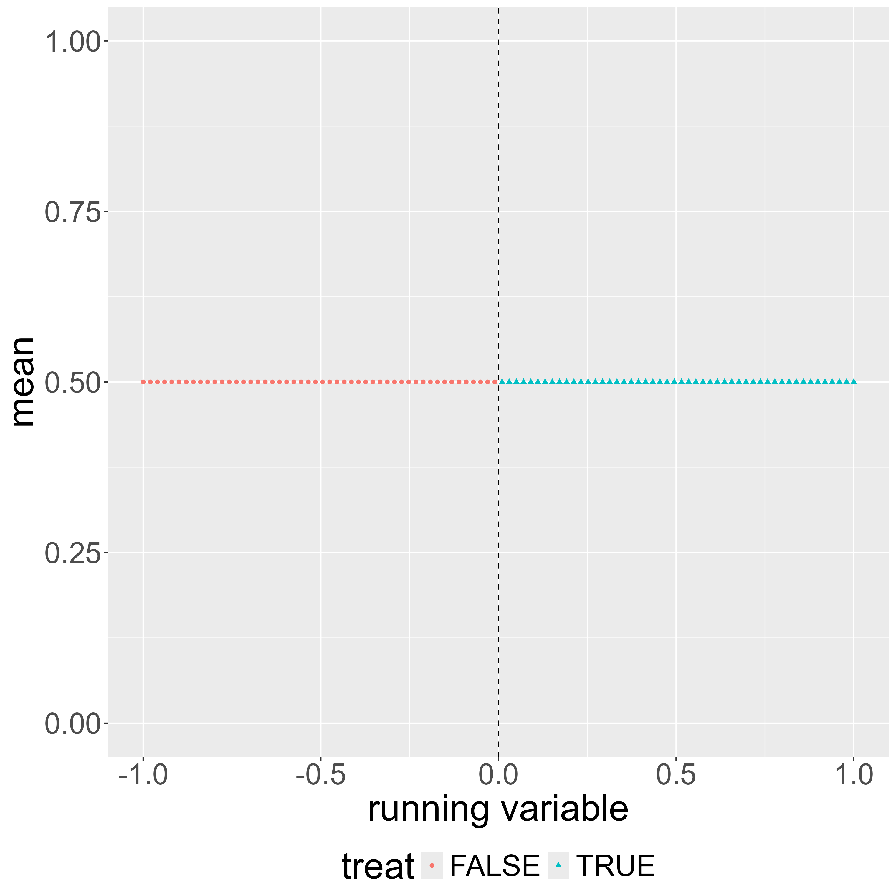
Figure 5.8: The flat model

We consider the estimation and inference of $\tau=p_{0,+}-p_{0,-}$. We use the true value of the Lipschitz constant $C$ for each design to implement our proposed method and the Gaussian method. Our proposed estimator for $\tau$ is given by $\hat{\tau}=\hat{p}_{0,+}(\hat{\bm{w}}_{+})-\hat{p}_{0,-}(\hat{\bm{w}}_{-})$, where $\hat{\bm{w}}_{+}$ and $\hat{\bm{w}}_{-}$ are chosen to minimize the worst-case MSE for the estimation of $p_{0,+}$ and $p_{0,-}$, respectively, as in Section 2. We then use $\hat{\tau}$ to construct a two-sided confidence interval for $\tau$, following the procedure in Section 4. An alternative, the Gaussian estimator, is $\tilde{\tau}=\hat{p}_{0,+}(\tilde{\bm{w}}_{+})-\hat{p}_{0,-}(\tilde{\bm{w}}_{-})$, where $\tilde{\bm{w}}_{+}$ and $\tilde{\bm{w}}_{-}$ minimize the worst-case MSE for the estimation of $p_{0,+}$ and $p_{0,-}$, respectively, under the misspecified model where $Y_{i}\sim N(p_{i},1/4)$, as in Section 3. Following Kolesár and Rothe (2018) and Armstrong and Kolesár (2021), we construct a two-sided fixed-length confidence interval centered at $\tilde{\tau}$, which has finite-sample validity under the Gaussian model. Specifically, the $100\cdot(1-\alpha)\%$ confidence interval is given by $\left(\tilde{\tau}\pm\rm{cv}_{\alpha}\left(\rm{maxbias}(\tilde{\tau})/\rm{sd}(\tilde{\tau})\right)\cdot\rm{sd}(\tilde{\tau})\right)$, where $\rm{maxbias}(\tilde{\tau})$ denotes the maximum bias of $\tilde{\tau}$ under the Lipschitz class and $\rm{cv}_{\alpha}(b)$ denotes the $1-\alpha$ quantile of $|N(b,1)|$, the folded normal distribution with location and scale parameters $(b,1)$.

First, we demonstrate the point estimation properties of our estimator. Tables 5.1 and 5.2 compare the root MSE and bias for the estimation of the ATE at the cutoff, computed from $3000$ replication draws. Table 5.1 compares three different sample sizes for the Lee model. For all sample sizes, our estimator has substantially smaller MSEs than the other estimators. Furthermore, the differences shrink as the sample size grows and the MSEs are relatively similar for $N=500$. The same pattern is confirmed for different designs that have different Lipschitz constants $C$. Hence, our estimator is superior to the existing estimators in small samples, while their behaviors resemble in larger samples.

In all three designs, our estimator is superior in the MSEs relative to the other existing methods. Note that our and Gaussian estimators use $C$ as if its true values are known. Nevertheless, the margin of differences is extraordinary for an extremely small sample size as $N=50$, and our estimator exhibits a favorable property in estimating the small sample RD designs.

Table 5.1: Simulation: point estimates (Lee)

	N = 50		N = 100		N = 500
	root		root		root
	MSE	Bias	MSE	Bias	MSE	Bias
rdbinary	0.264	0.063	0.223	0.067	0.141	0.065
gauss	0.302	0.124	0.248	0.107	0.149	0.078
rd.mnl	0.356	0.020	0.284	0.027	0.142	0.042
rdrobust	0.578	0.037	0.423	0.033	0.190	0.036

Table 5.2: Simulation: point estimates N=100

	worst_case		Lee		flat-50
	root		root		root
	MSE	Bias	MSE	Bias	MSE	Bias
rdbinary	0.239	0.136	0.223	0.067	0.088	0.000
gauss	0.288	0.205	0.248	0.107	0.100	0.000
rd.mnl	0.349	-0.006	0.284	0.027	0.253	-0.004
rdrobust	0.417	0.001	0.423	0.033	0.423	-0.004

Second, we demonstrate the inference properties of our estimator. Tables 5.3 and 5.4 compare the average length and coverage probability of the four confidence intervals, computed from $5000$ replication draws. In Table 5.3, we demonstrate that our confidence interval has shorter lengths with guaranteed coverage relative to rd.mnl and rdrobust for different sample sizes. Unlike in the point estimation results, the differences in lengths remain similar as the sample size grows. Note that the Gaussian confidence interval happened to have shorter lengths while achieving the $95\%$ coverage for the Lee design. Nevertheless, the Gaussian confidence interval does not guarantee the coverage as the coverage falls below $95\%$ for the flat design. This behavior is consistent with the fact that the Gaussian confidence interval is designed for the missspecified model where the outcomes, and hence linear estimators, follow normal distributions. Our confidence interval is, by construction, correctly specified for the binary dependent variable. Hence, our estimator is preferred when the outcome is known to be a binary variable. We also note that the rdrobust confidence interval is based on large-sample asymptotics and is not specifically designed for binary outcomes, resulting in unsatisfactory coverage properties in all designs with small samples.

Table 5.3: Simulation Results. DGP = Lee

	N = 50		N = 100		N = 500
	CI length	coverage	CI length	coverage	CI length	coverage
rdbinary	1.464	0.990	1.232	0.988	0.763	0.991
gauss	1.417	0.992	1.172	0.987	0.691	0.984
rd.mnl	1.712	0.946	1.625	0.953	1.161	0.967
rdrobust	1.615	0.888	1.481	0.906	0.814	0.929

Table 5.4: Simulation Results. N = 100

	worst_case		Lee		flat
	CI length	coverage	CI length	coverage	CI length	coverage
rdbinary	1.156	0.978	1.232	0.988	0.416	0.963
gauss	1.090	0.961	1.172	0.987	0.392	0.943
rd.mnl	1.455	0.932	1.625	0.953	1.667	0.968
rdrobust	1.469	0.908	1.481	0.906	1.498	0.906

5.2 Application

We apply our estimator to a small-sample RD study of Brollo et al. (2013). Brollo et al. (2013) exploit a regional fiscal rule in Brazil to study the impact of an additional government fiscal transfer on the frequency of corruption in local politics. In Brazil, 40 percent of the municipal revenue is the Fundo de Participação dos Municipios (FPM) which is allocated based on the population size of municipalities. Specifically, each municipality is allocated into one of nine brackets by their population levels. The bracketing fiscal rule induces population thresholds that discontinuously alter the amount of the FPM transfers. Following Brollo et al. (2013), we reduce the nine brackets into seven thresholds because of sample selection in municipalities that recorded their primary dependent variable of corruption measures.

We chose this study for two reasons. First, their primary dependent variables are binary indicators. Specificaly, they study the impact of the fiscal rule on two measures of corruption indicators:

broad corruption, which includes irregularities that could also be interpreted as bad administration rather than as overt corruption; and narrow corruption, which only includes severe irregularities that are also more likely to be visible to voters. (Brollo et al., 2013, page. 1774)

Second, their sample sizes are relatively small. Particularly within each cutoff neighborhood, the sample size is limited to less than $400$ and mostly around $100$ to $200$. In those small samples, our estimator is expected to be superior to other estimators that are based on asymptotic approximations.

The following tables exhibit our rdbinary estimates and rdrobust estimates. Tables 5.5 and 5.6 report the pooling estimates over multiple cutoffs for the broad and narrow corruption indicators. $Crot$ is a rule-of-thumb value for the Lipschitz constant $C$, which is the largest (in absolute value) slope estimate from the binscatter estimation by binsreg package (Cattaneo et al., 2024a). In all the tables, we report the point estimates and confidence intervals for three different values of the constant $C$: the rule-of-thumb $Crot$; one half of $Crot$; and $1.5$ times $Crot$.

estimator	C	point	CI
rdrobust		0.160	[-0.033, 0.325]
rdbinary	0.5*Crot	0.130	[-0.021, 0.283]
rdbinary	Crot	0.147	[-0.038, 0.342]
rdbinary	1.5*Crot	0.145	[-0.078, 0.368]

Table 5.5: Broad corruption pooled (N = 1202)

estimator	C	point	CI
rdrobust		0.164	[-0.054, 0.387]
rdbinary	0.5*Crot	0.131	[-0.011, 0.276]
rdbinary	Crot	0.154	[-0.024, 0.338]
rdbinary	1.5*Crot	0.155	[-0.057, 0.366]

Table 5.6: Narrow corruption pooled (N = 1202)

For both indicators, our rdbinary estimates appear similar to the rdrobust estimates, which are valid for large samples. The sample size is $1,202$ for the whole pooling sample and hence is large enough for the rdrobust estimator. For both methods and both outcomes, the $95\%$ confidence intervals include $0$. This finding is different from the original study, which reports significant positive impacts on the frequency of corruptions. This difference highlights the importance of applying local nonparametric estimations for RD designs.

By pooling samples across multiple cutoffs, we obtain a large enough sample across different cutoffs. Nevertheless, heterogeneity across different cutoffs may be of interest as the original study explores the cutoff-specific estimates. However, only a few hundreds of observations are around each individual cutoff. For such a small sample, the asymptotic approximation may not perform well.

Tables 5.7, 5.8, and 5.9 present our rdbinary and rdrobust estimates of the impact on the broad corruption for $7$ different subsamples around each individual cutoff. See Online Appendix for qualitatively similar results for the narrow corruption indicator. For all specifications, confidence intervals for each subsample are much wider than for the pooled sample. Nevertheless, our rdbinary estimates tend to offer much shorter confidence intervals than rdrobust estimates. For example, Cutoff 3 has a sample size of $225$, which is too small for rdrobust to have any insights from its estimate. On the other hand, our rdbinary estimates offer reasonable lower bounds for the impact on the broad corruption measure, which are not far negative compared to the lower bound of the confidence interval from rdrobust.

	Cutoff 1		Cutoff 2
estimator	point	CI	point	CI
rdrobust	0.038	[-0.372, 0.447]	0.057	[-0.307, 0.422]
rdbinary (0.5Crot)	0.075	[-0.128, 0.280]	0.168	[-0.186, 0.520]
rdbinary (Crot)	0.071	[-0.193, 0.337]	0.146	[-0.298, 0.576]
rdbinary (1.5Crot)	0.072	[-0.234, 0.375]	0.140	[-0.352, 0.632]

Table 5.7: Broad: at cutoffs 1 (N = 385) and 2 (N = 218)

	Cutoff 3		Cutoff 4
estimator	point	CI	point	CI
rdrobust	-0.099	[-0.533, 0.335]	0.058	[-0.572, 0.687]
rdbinary (0.5Crot)	0.192	[-0.088, 0.467]	-0.045	[-0.458, 0.364]
rdbinary (Crot)	0.228	[-0.117, 0.572]	-0.015	[-0.518, 0.469]
rdbinary (1.5Crot)	0.232	[-0.173, 0.635]	0.011	[-0.542, 0.570]

Table 5.8: Broad: at cutoffs 3 (N = 225) and 4 (N = 139)

	Cutoff 5		Cutoff 6		Cutoff 7
estimator	point	CI	point	CI	point	CI
rdrobust	0.719	[-0.863, 2.302]	-0.078	[-1.157, 1.000]	2.096	[-1.431, 5.623]
rdbinary (0.5Crot)	0.185	[-0.232, 0.607]	0.151	[-0.307, 0.603]	0.039	[-0.490, 0.567]
rdbinary (Crot)	0.279	[-0.263, 0.816]	0.109	[-0.458, 0.679]	0.199	[-0.512, 0.863]
rdbinary (1.5Crot)	0.330	[-0.312, 0.936]	0.081	[-0.586, 0.721]	0.246	[-0.563, 0.963]

Table 5.9: Broad: at cutoffs 5 (N = 116), 6 (N = 73), and 7 (N = 46)

6 Conclusion

Empirical studies often attempt using RD designs in small samples. However, estimation is challenging in small samples because their desired large-sample properties may be lost. A few finite-sample minimax estimators are proposed. However, those minimax estimators require the knowledge of the variance parameter, which is usually unknown.

In this study, we provide a minimax optimal estimator for RD designs with a binary outcome variable and its inference procedure. The key idea in our estimator is the following: all features of the conditional distribution, including the conditional variance, are a known function of the conditional mean function for a binary variable. For binary outcomes, our estimator relies on a single tuning parameter, the Lipschitz constant for the bound on the first derivative. Specifically, our estimator is free from specifying the conditional variance function, which is often required for minimax optimal estimators for RD designs. Our estimator is also applicable to any bounded outcome variable. Hence, we offer a practical finite-sample minimax optimal estimator for typical outcome variables, and our estimation can be the last resort for RD studies which have relatively small effective sample sizes.

We demonstrate that the estimator is superior to the existing estimators in finite samples in numerical and simulation exercises. In a numerical exercise, we show that our estimator is $5$ to $20$% more efficient in the worst-case root mean squared errors than the existing minimax optimal estimators for extremely small samples. In simulation studies, we show that our estimator has much smaller mean squared errors than the existing methods for small enough sample sizes. Furthermore, we demonstrate that our inference procedure generates shorter confidence intervals with guaranteed coverage rates than the existing methods. In the empirical application to a small-sample RD study, we document that our estimator generates similar results with the standard large-sample procedure for large enough samples but provides much more informative results for small enough samples.

Our contribution is a critical baseline for developing estimation procedures for a binary or limited outcome variable in RD designs. Recent studies such as Noack and Rothe (2024) consider bias-aware inference for fuzzy RD designs. As mentioned in Introduction, the binary treatment status is a primary dependent variable in the first stage of fuzzy designs. Applying our result is not necessarily straightforward as the first-stage estimand appears in the denominator of the target estimand. We reserve developing further extensions and generalizations of our results for future research.

Appendix A Proofs

Proof of Lemma 2.1.

Let $\tilde{\bm{\theta}}=(\theta_{0},\theta_{1}+2|\theta_{0}-\theta_{1}|_{+},\ldots,\theta_{n}+2|\theta_{0}-\theta_{n}|_{+})^{\prime}$, where $|a|_{+}\equiv\max\{a,0\}$. If $\theta_{i}\geq\theta_{0}$, then $\tilde{\theta}_{i}-\tilde{\theta}_{0}=\theta_{i}-\theta_{0}\geq 0$. If $\theta_{i}<\theta_{0}$, then $\tilde{\theta}_{i}-\tilde{\theta}_{0}=\theta_{i}+2(\theta_{0}-\theta_{i})-\theta_{0}=\theta_{0}-\theta_{i}\geq 0$. Hence, $\tilde{\bm{\theta}}$ satisfies $\tilde{\theta}_{i}\geq\tilde{\theta}_{0}$.

Next, we show $\tilde{\bm{\theta}}\in\Theta$. If $\theta_{i}\geq\theta_{0}$, then we have $\tilde{\theta}_{i}=\theta_{i}\in[-1/2,1/2]$. If $\theta_{i}<\theta_{0}$, then we have $\tilde{\theta}_{i}=\theta_{i}+2(\theta_{0}-\theta_{i})=\theta_{0}+(\theta_{0}-\theta_{i})\in[-1/2,1/2]$ because $\theta_{0}\in[-1/2,0]$ and $\theta_{0}-\theta_{i}\in[0,1/2]$. Hence, $\tilde{\bm{\theta}}\in[-1/2,1/2]^{n+1}$. It suffices to show that $|\tilde{\theta}_{i}-\tilde{\theta}_{j}|\leq C\|R_{i}-R_{j}\|$ for all $i$ and $j$. We consider the following three cases: (i) $\theta_{i}\geq\theta_{0}$ and $\theta_{j}\geq\theta_{0}$, (ii) $\theta_{i}\geq\theta_{0}$ and $\theta_{j}<\theta_{0}$, (iii) $\theta_{i}<\theta_{0}$ and $\theta_{j}<\theta_{0}$. In case (i), we have $|\tilde{\theta}_{i}-\tilde{\theta}_{j}|=|\theta_{i}-\theta_{j}|\leq C\|R_{i}-R_{j}\|$. In case (ii), we have

$$|\tilde{\theta}_{i}-\tilde{\theta}_{j}| = \left|\theta_{i}-(2\theta_{0}-\theta_{j})\right|\ =\ \left|(\theta_{i}-\theta_{0})+(\theta_{j}-\theta_{0})\right|$$

$$\leq (\theta_{i}-\theta_{0})+(\theta_{0}-\theta_{j})\ =\ (\theta_{i}-\theta_{j})\ \leq\ C\|R_{i}-R_{j}\|.$$

Similarly, in case (iii), we have

$$|\tilde{\theta}_{i}-\tilde{\theta}_{j}| = \left|(2\theta_{0}-\theta_{i})-(2\theta_{0}-\theta_{j})\right|\ =\ |\theta_{i}-\theta_{j}|\ \leq\ C\|R_{i}-R_{j}\|.$$

Therefore, we obtain $\tilde{\bm{\theta}}\in\Theta$.

Finally, we show that $\text{MSE}(\bm{w},\bm{\theta})\leq\text{MSE}(\bm{w},\tilde{\bm{\theta}})$. Because we have $\theta_{i}\leq\tilde{\theta}_{i}$ and $\tilde{\theta}_{0}=\theta_{0}$, we obtain $(\sum_{i=1}^{n}w_{i}\tilde{\theta}_{i}-\tilde{\theta}_{0})^{2}\geq(\sum_{i=1}^{n}w_{i}\theta_{i}-\theta_{0})^{2}$ when $\sum_{i=1}^{n}w_{i}\theta_{i}-\theta_{0}\geq 0$. In addition, as shown above, we have $\tilde{\theta}_{i}-\tilde{\theta}_{0}=|\theta_{i}-\theta_{0}|$ for all $i$. Because $\sum_{i=1}^{n}w_{i}\leq 1$ and $\theta_{0}\leq 0$, we obtain

$$\sum_{i=1}^{n}w_{i}\tilde{\theta}_{i}-\tilde{\theta}_{0} = \sum_{i=1}^{n}w_{i}(\tilde{\theta}_{i}-\tilde{\theta}_{0})-\left(1-\sum_{i=1}^{n}w_{i}\right)\theta_{0}\ \geq\ \sum_{i=1}^{n}w_{i}(\tilde{\theta}_{i}-\tilde{\theta}_{0})$$

$$= \sum_{i=1}^{n}w_{i}|\theta_{i}-\theta_{0}|\ \geq\ \sum_{i=1}^{n}w_{i}(\theta_{0}-\theta_{i})$$

$$= \theta_{0}-\sum_{i=1}^{n}w_{i}\theta_{i}-\left(1-\sum_{i=1}^{n}w_{i}\right)\theta_{0}\ \geq\ \theta_{0}-\sum_{i=1}^{n}w_{i}\theta_{i}.$$

This implies that $(\sum_{i=1}^{n}w_{i}\tilde{\theta}_{i}-\tilde{\theta}_{0})^{2}\geq(\sum_{i=1}^{n}w_{i}\theta_{i}-\theta_{0})^{2}$ also holds when $\sum_{i=1}^{n}w_{i}\theta_{i}-\theta_{0}\leq 0$. Furthermore, if $\theta_{i}<\theta_{0}$, then we have

$$\tilde{\theta}_{i}^{2} = (2\theta_{0}-\theta_{i})^{2}\ =\ \theta_{i}^{2}-4\theta_{0}\theta_{i}+4\theta_{0}^{2}\ =\ \theta_{i}^{2}+4\theta_{0}(\theta_{0}-\theta_{i})\ \leq\ \theta_{i}^{2}.$$

Because $\theta_{i}\geq\theta_{0}$ implies $\tilde{\theta}_{i}=\theta_{i}$, we obtain $1/4-\tilde{\theta}_{i}^{2}\geq 1/4-\theta_{i}^{2}$. Therefore, we obtain $\text{MSE}(\bm{w},\bm{\theta})\leq\text{MSE}(\bm{w},\tilde{\bm{\theta}})$. ∎

Proof of Theorem 2.1.

As discussed in Section 2.2, if $\bm{\theta}=(\theta_{0},\ldots,\theta_{n})^{\prime}\in\Theta$ satisfies (2.5), we obtain

$$\text{MSE}(\bm{w},\bm{\theta})\ \leq\ \text{MSE}(\bm{w},\tilde{\bm{\theta}}(\theta_{0}))\ \ \text{for all $\bm{w}\in\mathcal{W}$}.$$

Because $\tilde{\bm{\theta}}(\theta_{0})\in\Theta$ holds for all $\theta_{0}\in[-1/2,0]$, we obtain (2.7). ∎

Proof of Lemma 2.2.

Suppose that $\bm{w}\equiv(w_{1},\ldots,w_{n})^{\prime}\in\mathcal{W}$ satisfies $w_{j}<w_{j+1}$ for some $j$. Letting $\tilde{\bm{w}}\equiv(w_{1},\ldots,w_{j-1},w_{j+1},w_{j},w_{j+2},\ldots,w_{n})^{\prime}$, we have $\tilde{\bm{w}}\in\mathcal{W}$. For any $\bm{\theta}\in\Theta$, we observe that

$$\text{MSE}(\bm{w},\bm{\theta})-\text{MSE}(\tilde{\bm{w}},\bm{\theta})$$

$$= \left(\sum_{i=1}^{n}w_{i}\theta_{i}-\theta_{0}\right)^{2}-\left(\sum_{i=1}^{n}w_{i}\theta_{i}-w_{j}\theta_{j}-w_{j+1}\theta_{j+1}+w_{j+1}\theta_{j}+w_{j}\theta_{j+1}-\theta_{0}\right)^{2}$$

$$+w_{j}^{2}\left(1/4-\theta_{j}^{2}\right)+w_{j+1}^{2}\left(1/4-\theta_{j+1}^{2}\right)-w_{j+1}^{2}\left(1/4-\theta_{j}^{2}\right)-w_{j}^{2}\left(1/4-\theta_{j+1}^{2}\right)$$

$$= \left(\sum_{i=1}^{n}w_{i}\theta_{i}-\theta_{0}\right)^{2}-\left\{\left(\sum_{i=1}^{n}w_{i}\theta_{i}-\theta_{0}\right)-(w_{j}-w_{j+1})(\theta_{j}-\theta_{j+1})\right\}^{2}$$

$$-(w_{j}^{2}-w_{j+1}^{2})(\theta_{j}^{2}-\theta_{j+1}^{2})$$

$$= 2\left(\sum_{i=1}^{n}w_{i}\theta_{i}-\theta_{0}\right)(w_{j}-w_{j+1})(\theta_{j}-\theta_{j+1})-(w_{j}-w_{j+1})^{2}(\theta_{j}-\theta_{j+1})^{2}$$

$$-(w_{j}-w_{j+1})(\theta_{j}-\theta_{j+1})(w_{j}+w_{j+1})(\theta_{j}+\theta_{j+1})$$

$$= (w_{j}-w_{j+1})(\theta_{j}-\theta_{j+1})\left\{2\left(\sum_{i=1}^{n}w_{i}\theta_{i}-\theta_{0}\right)-2(w_{j}\theta_{j}+w_{j+1}\theta_{j+1})\right\}.$$

If $\bm{\theta}$ satisfies (2.5), we obtain

$$\left(\sum_{i=1}^{n}w_{i}\theta_{i}-\theta_{0}\right)-(w_{j}\theta_{j}+w_{j+1}\theta_{j+1})$$

$$= \sum_{i\neq j,\,j+1}w_{i}\theta_{i}-\theta_{0}\ \geq\ \left(\sum_{i\neq j,\,j+1}w_{i}-1\right)\theta_{0}\ \geq\ 0.$$

Because $\tilde{\bm{\theta}}(\theta_{0})$ satisfies (2.5) for all $\theta_{0}\in[-1/2,0]$, we obtain

$$\text{MSE}(\bm{w},\tilde{\bm{\theta}}(\theta_{0}))\ \geq\ \text{MSE}(\tilde{\bm{w}},\tilde{\bm{\theta}}(\theta_{0}))\ \ \text{for all $\theta_{0}\in[-1/2,0]$.}$$

It follows from Theorem 2.1 that we obtain

$$\max_{\bm{\theta}\in\Theta}\text{MSE}(\bm{w},\bm{\theta})\ \geq\ \max_{\bm{\theta}\in\Theta}\text{MSE}(\tilde{\bm{w}},\bm{\theta}).$$

Hence, if $w_{j}<w_{j+1}$, then we can reduce the maximum MSE by exchanging $w_{j}$ for $w_{j+1}$. Therefore, by repeating this procedure until the weight vector becomes monotone, we can obtain $\tilde{\bm{w}}\in\mathcal{W}_{0}$ such that $\max_{\bm{\theta}\in\Theta}\text{MSE}(\tilde{\bm{w}},\bm{\theta})\leq\max_{\bm{\theta}\in\Theta}\text{MSE}(\bm{w},\bm{\theta})$. ∎

Proof of Lemma 2.3.

We observe that

$$\frac{\partial}{\partial w_{j}}\text{MSE}(\bm{w},\bm{\theta}) = 2\theta_{j}\left(\sum_{i=1}^{n}w_{i}\theta_{i}-\theta_{0}\right)+2w_{j}\left(1/4-\theta_{j}^{2}\right)$$

$$= 2\theta_{j}\left(\sum_{i\neq j}w_{i}\theta_{i}-\theta_{0}\right)+w_{j}/2,$$

where $\sum_{i\neq j}w_{i}\theta_{i}-\theta_{0}\geq 0$ when (2.5) holds. If $\bm{\theta}$ satisfies (2.5) and $\theta_{j}\geq 0$, $\frac{\partial}{\partial w_{j}}\text{MSE}(\bm{w},\bm{\theta})$ is nonnegative for all $\bm{w}\in\mathcal{W}$. If $C\|R_{j}\|\geq 1/2$, then the $j$-th element of $\tilde{\bm{\theta}}(\theta_{0})$ is nonnegative for any $\theta_{0}\in[-1/2,0]$. Hence, we have

$$\frac{\partial}{\partial w_{j}}\text{MSE}(\bm{w},\tilde{\bm{\theta}}(\theta_{0}))\ \geq\ 0\ \ \text{for any $\theta_{0}\in[-1/2,0]$ and $\bm{w}\in\mathcal{W}$.}$$

Therefore, if $C\|R_{j}\|\geq 1/2$, then we obtain $\text{MSE}(\bm{w},\tilde{\bm{\theta}}(\theta_{0}))\geq\text{MSE}(\tilde{\bm{w}},\tilde{\bm{\theta}}(\theta_{0}))$, where $\tilde{\bm{w}}\equiv(w_{1},\ldots,w_{j-1},0,w_{j+1},\ldots,w_{n})^{\prime}$. As a result, combined with Lemma 2.2, we obtain $\min_{\bm{w}\in\mathcal{W}}\max_{\bm{\theta}\in\Theta}\text{MSE}(\bm{w},\bm{\theta})=\min_{\bm{w}\in\mathcal{W}_{1}}\max_{\bm{\theta}\in\Theta}\text{MSE}(\bm{w},\bm{\theta})$. ∎

Proof of Lemma 3.1.

Because $\hat{\bm{w}}$ minimizes $\max_{\bm{\theta}\in\Theta}\mathrm{MSE}(\bm{w},\bm{\theta})$, the lower bound is trivial. Hence, we consider the upper bound. Because $\mathrm{MSE}(\bm{w},\bm{\theta})\leq\mathrm{MSE}_{g}(\bm{w},\bm{\theta})$ and $\Theta\subset\Theta_{g}$, we have

$$\frac{\max_{\bm{\theta}\in\Theta}\mathrm{MSE}(\tilde{\bm{w}},\bm{\theta})}{\max_{\bm{\theta}\in\Theta}\mathrm{MSE}(\hat{\bm{w}},\bm{\theta})} \leq \frac{\max_{\bm{\theta}\in\Theta_{g}}\mathrm{MSE}_{g}(\tilde{\bm{w}},\bm{\theta})}{\max_{\bm{\theta}\in\Theta}\mathrm{MSE}(\hat{\bm{w}},\bm{\theta})}\ =\ \frac{\min_{\bm{w}\in\mathcal{W}}\max_{\bm{\theta}\in\Theta_{g}}\mathrm{MSE}_{g}(\bm{w},\bm{\theta})}{\min_{\bm{w}\in\mathcal{W}}\max_{\bm{\theta}\in\Theta}\mathrm{MSE}(\bm{w},\bm{\theta})}.$$

First, we derive a lower bound of $\min_{\bm{w}\in\mathcal{W}}\max_{\bm{\theta}\in\Theta}\mathrm{MSE}(\bm{w},\bm{\theta})$. From Theorem 2.1 and Lemmas 2.2–2.3, we obtain

$$\min_{\bm{w}\in\mathcal{W}}\max_{\bm{\theta}\in\Theta}\mathrm{MSE}(\bm{w},\bm{\theta}) = \max_{\theta_{0}\in[-1/2,0]}\mathrm{MSE}(\hat{\bm{w}},\tilde{\bm{\theta}}(\theta_{0}))\ \geq\ \mathrm{MSE}(\hat{\bm{w}},\tilde{\bm{\theta}}(0))$$

$$= C^{2}\left(\sum_{i=1}^{n}\hat{w}_{i}\|R_{i}\|\right)^{2}+\sum_{i=1}^{n}\hat{w}_{i}^{2}\left(\frac{1}{4}-C^{2}\|R_{i}\|^{2}\right).$$

Next, we derive an upper bound of $\min_{\bm{w}\in\mathcal{W}}\max_{\bm{\theta}\in\Theta_{g}}\mathrm{MSE}_{g}(\bm{w},\bm{\theta})$. If $\bm{w}\in\mathcal{W}$ satisfies $\sum_{i=1}^{n}w_{i}=1$, then $\max_{\bm{\theta}\in\Theta_{g}}\mathrm{MSE}_{g}(\bm{w},\bm{\theta})$ can be written as follows:

$$\max_{\bm{\theta}\in\Theta_{g}}\mathrm{MSE}_{g}(\bm{w},\bm{\theta})\ =\ C^{2}\left(\sum_{i=1}^{n}w_{i}\|R_{i}\|\right)^{2}+\frac{1}{4}\sum_{i=1}^{n}w_{i}^{2}.$$

Because $\tilde{\bm{w}}$ satisfies $\sum_{i=1}^{n}\tilde{w}_{i}=1$, we obtain

$$\min_{\bm{w}\in\mathcal{W}}\max_{\bm{\theta}\in\Theta_{g}}\mathrm{MSE}_{g}(\bm{w},\bm{\theta}) = \min_{\bm{w}\in\mathcal{W}:\sum_{i=1}^{n}w_{i}=1}\max_{\bm{\theta}\in\Theta_{g}}\mathrm{MSE}_{g}(\bm{w},\bm{\theta})$$

$$= \min_{\bm{w}\in\mathcal{W}:\sum_{i=1}^{n}w_{i}=1}\left\{C^{2}\left(\sum_{i=1}^{n}w_{i}\|R_{i}\|\right)^{2}+\frac{1}{4}\sum_{i=1}^{n}w_{i}^{2}\right\}$$

$$\leq C^{2}\left(\sum_{i=1}^{n}(\hat{w}_{i}/\hat{u})\|R_{i}\|\right)^{2}+\frac{1}{4}\sum_{i=1}^{n}(\hat{w}_{i}/\hat{u})^{2}$$

$$= \hat{u}^{-2}\left\{C^{2}\left(\sum_{i=1}^{n}\hat{w}_{i}\|R_{i}\|\right)^{2}+\frac{1}{4}\sum_{i=1}^{n}\hat{w}_{i}^{2}\right\}.$$

Therefore, we obtain

$$\frac{\max_{\bm{\theta}\in\Theta}\mathrm{MSE}(\tilde{\bm{w}},\bm{\theta})}{\max_{\bm{\theta}\in\Theta}\mathrm{MSE}(\hat{\bm{w}},\bm{\theta})} \leq \left(1+\frac{C^{2}\sum_{i=1}^{n}\hat{w}_{i}^{2}\|R_{i}\|^{2}}{C^{2}\left(\sum_{i=1}^{n}\hat{w}_{i}\|R_{i}\|\right)^{2}+\sum_{i=1}^{n}\hat{w}_{i}^{2}\left(\frac{1}{4}-C^{2}\|R_{i}\|^{2}\right)}\right)\hat{u}^{-2}$$

$$= \left(1+\frac{C^{2}\sum_{i=1}^{n}\hat{w}_{i}^{2}\|R_{i}\|^{2}}{C^{2}\sum_{i\neq j}\hat{w}_{i}\hat{w}_{j}\|R_{i}\|\|R_{j}\|+\frac{1}{4}\sum_{i=1}^{n}\hat{w}_{i}^{2}}\right)\hat{u}^{-2}$$

$$\leq \left(1+\frac{C^{2}\sum_{i=1}^{n}\hat{w}_{i}^{2}\|R_{i}\|^{2}}{\frac{1}{4}\sum_{i=1}^{n}\hat{w}_{i}^{2}}\right)\hat{u}^{-2}.$$

Because $\hat{w}_{i}=0$ holds if $C\|R_{i}\|\geq 1/2$, we have $C^{2}\sum_{i=1}^{n}\hat{w}_{i}^{2}\|R_{i}\|^{2}\leq\frac{1}{4}\sum_{i=1}^{n}\hat{w}_{i}^{2}$. As a result, the upper bound of (3.2) is bounded above by $2\hat{u}^{-2}$. ∎

Proof of Theorem 3.1.

We consider a sufficiently large $n\in\mathbb{N}$ such that $c_{0}x-n^{-\alpha}\leq F_{n}(x)\leq c_{1}x+n^{-\alpha}$ for all $x\in[0,1]$ with $\alpha=1/3$. For any $\epsilon>0$, let $N(\epsilon)\equiv\max\{i\in\{1,\ldots,n\}:\|R_{i}\|\leq\epsilon\}$. Because $\|R_{1}\|\leq\cdots\leq\|R_{n}\|$, we have $N(\epsilon)=nF_{n}(\epsilon)$ for $\epsilon\in(0,1]$. Hence, under Assumption 3.1, we obtain

$$c_{0}n\epsilon-n^{1-\alpha}\ \leq\ N(\epsilon)\ \leq\ c_{1}n\epsilon+n^{1-\alpha},\ \ \ \forall\epsilon\in(0,1].$$

First, we discuss the convergence rate of $\hat{p}_{0}(\hat{\bm{w}})$. Since $\mathrm{MSE}(\bm{w},\bm{\theta})\leq\mathrm{MSE}_{g}(\bm{w},\bm{\theta})$ and $\Theta\subset\Theta_{g}$, we have

$$\max_{\bm{\theta}\in\Theta}\mathrm{MSE}(\hat{\bm{w}},\bm{\theta}) = \min_{\bm{w}\in\mathcal{W}}\max_{\bm{\theta}\in\Theta}\mathrm{MSE}(\bm{w},\bm{\theta})$$

$$\leq \min_{\bm{w}\in\mathcal{W}}\max_{\bm{\theta}\in\Theta_{g}}\mathrm{MSE}_{g}(\bm{w},\bm{\theta})\ =\ \max_{\bm{\theta}\in\Theta_{g}}\mathrm{MSE}_{g}(\tilde{\bm{w}},\bm{\theta}).$$

This implies that if $\max_{\bm{\theta}\in\Theta_{g}}\mathrm{MSE}_{g}(\tilde{\bm{w}},\bm{\theta})$ converges to zero as $n\rightarrow\infty$, $\max_{\bm{\theta}\in\Theta}\mathrm{MSE}(\hat{\bm{w}},\bm{\theta})$ converges to zero no slower than $\max_{\bm{\theta}\in\Theta_{g}}\mathrm{MSE}_{g}(\tilde{\bm{w}},\bm{\theta})$. If $2c_{0}^{-1}n^{-\alpha}\leq\epsilon\leq 1$, then $N(\epsilon)\geq c_{0}n\epsilon-n^{1-\alpha}\geq n^{1-\alpha}>0$, and we obtain

$$\max_{\bm{\theta}\in\Theta_{g}}\mathrm{MSE}_{g}(\tilde{\bm{w}},\bm{\theta}) = \min_{\bm{w}\in\mathcal{W}:\sum_{i=1}^{n}w_{i}=1}\max_{\bm{\theta}\in\Theta_{g}}\mathrm{MSE}_{g}(\bm{w},\bm{\theta})$$

$$= \min_{\bm{w}\in\mathcal{W}:\sum_{i=1}^{n}w_{i}=1}\left\{C^{2}\left(\sum_{i=1}^{n}w_{i}\|R_{i}\|\right)^{2}+\frac{1}{4}\sum_{i=1}^{n}w_{i}^{2}\right\}$$

$$\leq C^{2}\left(\frac{1}{N(\epsilon)}\sum_{i=1}^{N(\epsilon)}\|R_{i}\|\right)^{2}+\frac{1}{4N(\epsilon)}$$

$$\leq C^{2}\epsilon^{2}+\frac{1}{4N(\epsilon)}\ \leq\ C^{2}\epsilon^{2}+\frac{1}{4(c_{0}n\epsilon-n^{1-\alpha})},$$

where the first equality holds since $\tilde{\bm{w}}$ satisfies $\sum_{i=1}^{n}\tilde{w}_{i}=1$, the first inequality follows by setting

$$\bm{w}=\left(\underbrace{\frac{1}{N(\epsilon)},\ldots,\frac{1}{N(\epsilon)}}_{N(\epsilon)},0,\ldots,0\right)^{\prime},$$

and the second inequality holds since $\|R_{i}\|\leq\epsilon$ for $i=1,\dots,N(\epsilon)$. If we set $\epsilon=O(n^{-1/3})$ satisfying $\epsilon\geq 2c_{0}^{-1}n^{-\alpha}$, which exists for $\alpha\geq 1/3$, then the right-hand side becomes $O(n^{-2/3})$. For example, if we set $\epsilon=2c_{0}^{-1}n^{-1/3}$, which satisfies $\epsilon\geq 2c_{0}^{-1}n^{-\alpha}$ for $\alpha\geq 1/3$, then the right-hand side becomes

$$4C^{2}c_{0}^{-2}n^{-2/3}+\frac{1}{4(2n^{2/3}-n^{1-\alpha})}=\left(4C^{2}c_{0}^{-2}+\frac{1}{4(2-n^{1/3-\alpha})}\right)n^{-2/3}=O(n^{-2/3}).$$

Hence, $\max_{\bm{\theta}\in\Theta}\mathrm{MSE}(\hat{\bm{w}},\bm{\theta})=O(n^{-2/3})$.

Next, we show that $\frac{\max_{\bm{\theta}\in\Theta}\text{MSE}(\tilde{\bm{w}},\bm{\theta})}{\max_{\bm{\theta}\in\Theta}\text{MSE}(\hat{\bm{w}},\bm{\theta})}\ \to\ 1$. For any $\bm{w}\in\mathcal{W}$, we observe that

$$\max_{\bm{\theta}\in\Theta}\mathrm{MSE}(\hat{\bm{w}},\bm{\theta}) \geq \max_{\bm{\theta}\in\Theta}\left(\sum_{i=1}^{n}\hat{w}_{i}\theta_{i}-\theta_{0}\right)^{2}\ \geq\ \max_{\bm{\theta}\in\Theta:\theta_{0}=-1/2}\left(\sum_{i=1}^{n}\hat{w}_{i}\theta_{i}+\frac{1}{2}\right)^{2}$$

$$= \max_{\bm{\theta}\in\Theta:\theta_{0}=-1/2}\left\{\sum_{i=1}^{n}\hat{w}_{i}(\theta_{i}+1/2)+\frac{1}{2}\left(1-\sum_{i=1}^{n}\hat{w}_{i}\right)\right\}^{2}$$

$$\geq \frac{1}{4}\left(1-\sum_{i=1}^{n}\hat{w}_{i}\right)^{2}\ =\ \frac{1}{4}\left(1-\hat{u}\right)^{2},$$

where the last inequality follows from $\theta_{i}+1/2\geq 0$. This implies that $\hat{u}$ converges to one because $\max_{\bm{\theta}\in\Theta}\mathrm{MSE}(\hat{\bm{w}},\bm{\theta})$ converges to zero. From Lemma 3.1, we obtain

$$1\ \leq\ \frac{\max_{\bm{\theta}\in\Theta}\mathrm{MSE}(\tilde{\bm{w}},\bm{\theta})}{\max_{\bm{\theta}\in\Theta}\mathrm{MSE}(\hat{\bm{w}},\bm{\theta})}\ \leq\ \left(1+\frac{C^{2}\sum_{i=1}^{n}\hat{w}_{i}^{2}\|R_{i}\|^{2}}{\frac{1}{4}\sum_{i=1}^{n}\hat{w}_{i}^{2}}\right)\hat{u}^{-2}.$$

Hence, it suffices to show that

$$\frac{C^{2}\sum_{i=1}^{n}\hat{w}_{i}^{2}\|R_{i}\|^{2}}{\frac{1}{4}\sum_{i=1}^{n}\hat{w}_{i}^{2}}\ \to\ 0.$$ (A.1)

If $2c_{0}^{-1}n^{-\alpha}\leq\epsilon\leq 1$, we can bound the left-hand side of (A.1) as follows:

$$\frac{C^{2}\sum_{i=1}^{n}\hat{w}_{i}^{2}\|R_{i}\|^{2}}{\frac{1}{4}\sum_{i=1}^{n}\hat{w}_{i}^{2}} = \frac{4C^{2}\sum_{i=1}^{N(\epsilon)}\hat{w}_{i}^{2}\|R_{i}\|^{2}+4C^{2}\sum_{i=N(\epsilon)+1}^{n}\hat{w}_{i}^{2}\|R_{i}\|^{2}}{\sum_{i=1}^{n}\hat{w}_{i}^{2}}$$ (A.2)

$$\leq 4C^{2}\left\{\frac{\epsilon^{2}\left(\sum_{i=1}^{N(\epsilon)}\hat{w}_{i}^{2}\right)+\hat{w}_{N(\epsilon)}^{2}\left(\sum_{i=N(\epsilon)+1}^{n}\|R_{i}\|^{2}\right)}{\sum_{i=1}^{n}\hat{w}_{i}^{2}}\right\}$$

$$\leq 4C^{2}\left\{\epsilon^{2}+\frac{n\hat{w}_{N(\epsilon)}^{2}}{\sum_{i=1}^{n}\hat{w}_{i}^{2}}\right\},$$

where the first inequality follows since $\|R_{i}\|\leq\epsilon$ for $i=1,\dots,N(\epsilon)$ and $\hat{w}_{i}\leq\hat{w}_{N(\epsilon)}$ for $i=N(\epsilon)+1,\ldots,n$, and the second inequality follows since $\|R_{1}\|\leq\ldots\leq\|R_{n}\|\leq 1$.

To further bound the right-hand side of (A.2), we obtain a lower bound on $\sum_{i=1}^{n}\hat{w}_{i}^{2}$ and an upper bound on $\hat{w}_{N(\epsilon)}^{2}$. A lower bound on $\sum_{i=1}^{n}\hat{w}_{i}^{2}$ is given by

$$\sum_{i=1}^{n}\hat{w}_{i}^{2}=\hat{u}^{2}\sum_{i=1}^{n}(\hat{w}_{i}/\hat{u})^{2}\geq\hat{u}^{2}n^{-1},$$

where the inequality follows from the fact that $\sum_{i=1}^{n}w_{i}^{2}\geq n^{-1}$ for any $(w_{1},\ldots,w_{n})\in\mathbb{R}^{n}$ such that $\sum_{i=1}^{n}w_{i}=1$. To obtain an upper bound on $\hat{w}_{N(\epsilon)}^{2}$, we observe that, if $2c_{0}^{-1}n^{-\alpha}\leq\epsilon\leq 1$,

$$O(n^{-2/3}) = \max_{\bm{\theta}\in\Theta}\text{MSE}(\hat{\bm{w}},\bm{\theta})\ \geq\ \text{MSE}(\hat{\bm{w}},\tilde{\bm{\theta}}(0))$$

$$\geq C^{2}\left(\sum_{i=1}^{n}\hat{w}_{i}\|R_{i}\|\right)^{2}\ \geq\ C^{2}\hat{w}_{N(\epsilon)}^{2}\left(\sum_{i=1}^{N(\epsilon)}\|R_{i}\|\right)^{2},$$

where the second and third inequalities follow from Lemmas 2.3 and 2.2, respectively. Below, we show that, if $\epsilon>2c_{0}^{-1}n^{-\alpha}$, then $\sum_{i=1}^{N(\epsilon)}\|R_{i}\|\geq\frac{(N(\epsilon)-n^{1-\alpha})^{2}}{2c_{1}n}$. Once it is shown, it follows from the assumption $N(\epsilon)\geq c_{0}n\epsilon-n^{1-\alpha}$ that

$$O(n^{-2/3}) \geq C^{2}\hat{w}_{N(\epsilon)}^{2}\frac{(N(\epsilon)-n^{1-\alpha})^{4}}{4c_{1}^{2}n^{2}}$$

$$\geq C^{2}\hat{w}_{N(\epsilon)}^{2}\frac{(c_{0}n\epsilon-2n^{1-\alpha})^{4}}{4c_{1}^{2}n^{2}}=\frac{C^{2}}{4c_{1}^{2}}\hat{w}_{N(\epsilon)}^{2}(c_{0}n^{1/2}\epsilon-2n^{1/2-\alpha})^{4},$$

which implies that there exists $c_{2}>0$ (which is independent of $\epsilon$ and $n$) such that

$$\hat{w}_{N(\epsilon)}^{2}\leq\frac{c_{2}n^{-2/3}}{(c_{0}n^{1/2}\epsilon-2n^{1/2-\alpha})^{4}}\ \ \text{if }\epsilon>2c_{0}^{-1}n^{-\alpha}.$$

Now we show the aforementioned claim: if $\epsilon>2c_{0}^{-1}n^{-\alpha}$, $\sum_{i=1}^{N(\epsilon)}\|R_{i}\|\geq\frac{(N(\epsilon)-n^{1-\alpha})^{2}}{2c_{1}n}$. Let $x^{*}(\epsilon)\equiv\frac{N(\epsilon)-n^{1-\alpha}}{c_{1}n}$, which is the unique solution to $c_{1}nx+n^{1-\alpha}=N(\epsilon)$ with respect to $x$. If $\epsilon>2c_{0}^{-1}n^{-\alpha}$, we must have $0<x^{*}(\epsilon)\leq\|R_{N(\epsilon)}\|$, since $c_{1}n\cdot 0+n^{1-\alpha}<c_{0}n\epsilon-n^{1-\alpha}\leq N(\epsilon)$ and $c_{1}n\|R_{N(\epsilon)}\|+n^{1-\alpha}\geq N(\|R_{N(\epsilon)}\|)=N(\epsilon)$ under Assumption 3.1. Here, $N(\|R_{N(\epsilon)}\|)=N(\epsilon)$ holds by the definition of $N(\epsilon)$. Also, let

$$g_{\epsilon}(x)\equiv\begin{cases}c_{1}nx+n^{1-\alpha}&\text{if }0<x\leq x^{*}(\epsilon),\\ N(\epsilon)&\text{if }x^{*}(\epsilon)<x\leq 1.\end{cases}$$

Note that $g_{\epsilon}(x)\geq N(x)$ for all $x\in(0,\|R_{N(\epsilon)}\|]$, since $g_{\epsilon}(x)=c_{1}nx+n^{1-\alpha}\geq N(x)$ if $0<x\leq x^{*}(\epsilon)$ by Assumption 3.1 and $g_{\epsilon}(x)=N(\epsilon)=N(\|R_{N(\epsilon)}\|)\geq N(x)$ if $x^{*}(\epsilon)<x\leq\|R_{N(\epsilon)}\|$. Therefore, we have

$$\int_{0}^{\|R_{N(\epsilon)}\|}(N(\epsilon)-N(x))dx\geq\int_{0}^{\|R_{N(\epsilon)}\|}(N(\epsilon)-g_{\epsilon}(x))dx.$$

We calculate each of both sides of the above inequality:

$$\int_{0}^{\|R_{N(\epsilon)}\|}(N(\epsilon)-N(x))dx$$

$$=\int_{0}^{\|R_{1}\|}(N(\epsilon)-0)dx+\int_{\|R_{1}\|}^{\|R_{2}\|}(N(\epsilon)-1)dx+\cdots+\int_{\|R_{N(\epsilon)-1}\|}^{\|R_{N(\epsilon)}\|}(N(\epsilon)-(N(\epsilon)-1))dx$$

$$=N(\epsilon)\|R_{1}\|+(N(\epsilon)-1)(\|R_{2}\|-\|R_{1}\|)+\cdots+(\|R_{N(\epsilon)}\|-\|R_{N(\epsilon)-1}\|)$$

$$=\sum_{i=1}^{N(\epsilon)}\|R_{i}\|$$

and

$$\int_{0}^{\|R_{N(\epsilon)}\|}(N(\epsilon)-g_{\epsilon}(x))dx = \int_{0}^{x^{*}(\epsilon)}(N(\epsilon)-c_{1}nx-n^{1-\alpha})dx=\frac{(N(\epsilon)-n^{1-\alpha})^{2}}{2c_{1}n}.$$

Thus, we obtain $\sum_{i=1}^{N(\epsilon)}\|R_{i}\|\geq\frac{(N(\epsilon)-n^{1-\alpha})^{2}}{2c_{1}n}$. See Figure A.1 for the intuition for this argument.

Figure A.1: The blue solid line denotes a function $y=\max\{i:\|R_{i}\|\leq x\}$ and the blue dotted line denotes a function $y=c_{1}nx+n^{1-\alpha}$. The area of the gray region is $\sum_{i=1}^{N(\epsilon)}\|R_{i}\|$ and the area of the shaded triangle is $\frac{(N(\epsilon)-n^{1-\alpha})^{2}}{2c_{1}n}$.

Finally, combining the lower bound on $\sum_{i=1}^{n}\hat{w}_{i}^{2}$ and the upper bound on $\hat{w}_{N(\epsilon)}^{2}$ obtained above yields the following bound on the right-hand side of (A.2): if $\epsilon>2c_{0}^{-1}n^{-\alpha}$,

$$4C^{2}\left\{\epsilon^{2}+\frac{n\hat{w}_{N(\epsilon)}^{2}}{\sum_{i=1}^{n}\hat{w}_{i}^{2}}\right\} \leq 4C^{2}\left\{\epsilon^{2}+\frac{c_{2}n^{4/3}}{(c_{0}n^{1/2}\epsilon-2n^{1/2-\alpha})^{4}}\hat{u}^{-2}\right\}$$

$$= 4C^{2}\left\{\epsilon^{2}+\frac{c_{2}}{(c_{0}n^{1/6}\epsilon-2n^{1/6-\alpha})^{4}}\hat{u}^{-2}\right\}.$$

If we set $\epsilon=n^{-\beta}$ for some $0<\beta<\min\{1/6,\alpha\}$ (which is equivalent to $0<\beta<1/6$ as $\alpha=1/3$), then $\epsilon>2c_{0}^{-1}n^{-\alpha}$ for any sufficiently large $n$, and we have

$$4C^{2}\left\{\epsilon^{2}+\frac{c_{2}}{(c_{0}n^{1/6}\epsilon-2n^{1/6-\alpha})^{4}}\hat{u}^{-2}\right\}=4C^{2}\left\{n^{-2\beta}+\frac{c_{2}}{(c_{0}n^{1/6-\beta}-2n^{1/6-\alpha})^{4}}\hat{u}^{-2}\right\}=o(1).$$

Therefore, we obtain the desired result because (A.1) holds.

∎

Proof of Theorem 4.1.

Fix $\bm{p}=(\bm{p}_{+}^{\prime},\bm{p}_{-}^{\prime})^{\prime}=(p_{0,+},\ldots,p_{n_{+},+},p_{0,-},\ldots,p_{n_{-},-})^{\prime}\in\mathcal{P}(\tau_{0})$. Define

$$\bm{Y} \equiv (Y_{1,+},\ldots,Y_{n_{+},+},Y_{1,-},\ldots,Y_{n_{-},-})^{\prime},$$

$$\tilde{\bm{Y}} \equiv (\tilde{Y}_{1,+},\ldots,\tilde{Y}_{n_{+},+},\tilde{Y}_{1,-},\ldots,\tilde{Y}_{n_{-},-})^{\prime},$$

$$\hat{\tau}(\bm{Y}) \equiv \sum_{i=1}^{n_{+}}w_{i,+}\left(Y_{i,+}-\frac{1}{2}\right)-\sum_{i=1}^{n_{-}}w_{i,-}\left(Y_{i,-}-\frac{1}{2}\right),$$

where $\bm{Y}$ and $\tilde{\bm{Y}}$ follow Bernoulli distribution with parameters $\bm{p}$ and $\tilde{\bm{p}}(p_{0,+},\tau_{0})$, respectively. Then, $\hat{\tau}(\bm{Y})$ is increasing function in $Y_{i,+}$ and decreasing in $Y_{i,-}$. Because $\tilde{Y}_{i,+}$ has first-order stochastic dominance over $Y_{i,+}$ and $-\tilde{Y}_{i,-}$ has first-order stochastic dominance over $-Y_{i,-}$, it follows from Lemma 1 of Ishihara (2023) that we have

$$P(\hat{\tau}(\bm{Y})>\gamma)\ \leq\ P(\hat{\tau}(\tilde{\bm{Y}})>\gamma).$$

In addition, we have $\tilde{\bm{p}}(p,\tau_{0})\in\mathcal{P}(\tau_{0})$ for any $p\in[\max\{0,\tau_{0}\},\min\{1,1+\tau_{0}\}]$. Hence, we obtain (4.2). ∎

Appendix B Minimax estimation for the average treatment effect

In this section, we consider the same setting in Remark 2.5 at the end of Section 2 and provide how to compute the maximum MSE for the ATE. We consider the following estimator of the ATE:

$$\hat{\tau}(\bm{w}_{+},\bm{w}_{-}) \equiv \hat{p}_{0,+}(\bm{w}_{+})-\hat{p}_{0,-}(\bm{w}_{-})\ =\ \sum_{i=1}^{n_{+}}w_{i,+}\left(Y_{i,+}-\frac{1}{2}\right)-\sum_{i=1}^{n_{-}}w_{i,-}\left(Y_{i,-}-\frac{1}{2}\right),$$

where $\bm{w}_{+}\equiv(w_{1,+},\ldots,w_{n_{+},+})^{\prime}$ and $\bm{w}_{-}\equiv(w_{1,-},\ldots,w_{n_{-},-})^{\prime}$. Similar to Section 2, we assume that $\bm{w}_{+}\in\mathcal{W}_{+}$ and $\bm{w}_{-}\in\mathcal{W}_{-}$ hold, where

$$\mathcal{W}_{+} \equiv \left\{\bm{w}_{+}\in\mathbb{R}^{n_{+}}:\sum_{i=1}^{n_{+}}w_{i,+}\leq 1\ \text{and}\ w_{i,+}\geq 0\ \text{for all $i$}\right\},$$

$$\mathcal{W}_{-} \equiv \left\{\bm{w}_{-}\in\mathbb{R}^{n_{-}}:\sum_{i=1}^{n_{-}}w_{i,-}\leq 1\ \text{and}\ w_{i,-}\geq 0\ \text{for all $i$}\right\}.$$

Suppose that $Y_{i,+}$ and $Y_{i,-}$ follow Bernoulli distribution with parameters $p_{i,+}$ and $p_{i,-}$, respectively. Letting $\theta_{i,+}\equiv p_{i,+}-1/2$, $\theta_{i,-}\equiv p_{i,-}-1/2$, $\bm{\theta}_{+}\equiv(\theta_{0,+},\ldots,\theta_{n_{+},+})^{\prime}$, and $\bm{\theta}_{-}\equiv(\theta_{0,-},\ldots,\theta_{n_{-},-})^{\prime}$, we consider the following parameter spaces:

$$\Theta_{+} \equiv \left\{\bm{\theta}_{+}\in[-1/2,1/2]^{n_{+}+1}:|\theta_{i,+}-\theta_{j,+}|\leq C\|R_{i,+}-R_{j,+}\|\ \text{for all $i$ and $j$}\right\},$$

$$\Theta_{-} \equiv \left\{\bm{\theta}_{-}\in[-1/2,1/2]^{n_{-}+1}:|\theta_{i,-}-\theta_{j,-}|\leq C\|R_{i,-}-R_{j,-}\|\ \text{for all $i$ and $j$}\right\},$$

where $R_{0,+}=R_{0,-}=0$. Similar to Section 2, we assume $\|R_{0,+}\|\leq\|R_{1,+}\|\leq\cdots\leq\|R_{n_{+},+}\|$ and $\|R_{0,-}\|\leq\|R_{1,-}\|\leq\cdots\leq\|R_{n_{-},-}\|$.

Because the ATE is $\tau\equiv\theta_{0,+}-\theta_{0,-}$, the MSE of $\hat{\tau}(\bm{w}_{+},\bm{w}_{-})$ can be written as follows:

$$\text{MSE}_{ate}(\bm{w}_{+},\bm{w}_{-},\bm{\theta}_{+},\bm{\theta}_{-})\ \equiv\ E\left[\left\{\hat{\tau}(\bm{w}_{+},\bm{w}_{-})-\tau\right\}^{2}\right]$$

$$= E\left[\left\{\sum_{i=1}^{n_{+}}w_{i,+}\left(Y_{i,+}-\frac{1}{2}\right)-\theta_{0,+}\right\}^{2}\right]+E\left[\left\{\sum_{i=1}^{n_{-}}w_{i,-}\left(Y_{i,-}-\frac{1}{2}\right)-\theta_{0,-}\right\}^{2}\right]$$

$$\hskip 57.81621pt-2E\left[\left\{\sum_{i=1}^{n_{+}}w_{i,+}\left(Y_{i,+}-\frac{1}{2}\right)-\theta_{0,+}\right\}\left\{\sum_{i=1}^{n_{-}}w_{i,-}\left(Y_{i,-}-\frac{1}{2}\right)-\theta_{0,-}\right\}\right]$$

$$= b_{+}(\bm{w}_{+},\bm{\theta}_{+})^{2}+V_{+}(\bm{w}_{+},\bm{\theta}_{+})$$

$$\hskip 36.135pt+b_{-}(\bm{w}_{-},\bm{\theta}_{-})^{2}+V_{-}(\bm{w}_{-},\bm{\theta}_{-})-2b_{+}(\bm{w}_{+},\bm{\theta}_{+})b_{-}(\bm{w}_{-},\bm{\theta}_{-}),$$

where

$$b_{+}(\bm{w}_{+},\bm{\theta}_{+})\equiv\sum_{i=1}^{n_{+}}w_{i,+}\theta_{i,+}-\theta_{0,+},\ \ \ \ V_{+}(\bm{w}_{+},\bm{\theta}_{+})\equiv\sum_{i=1}^{n_{+}}w_{i,+}^{2}\left(\frac{1}{4}-\theta_{i,+}^{2}\right),$$

$$b_{-}(\bm{w}_{-},\bm{\theta}_{-})\equiv\sum_{i=1}^{n_{-}}w_{i,-}\theta_{i,-}-\theta_{0,-},\ \ \ \ V_{-}(\bm{w}_{-},\bm{\theta}_{-})\equiv\sum_{i=1}^{n_{-}}w_{i,-}^{2}\left(\frac{1}{4}-\theta_{i,-}^{2}\right).$$

We define

$$\tilde{\bm{\theta}}_{+}(\theta_{0,+}) \equiv \left(\theta_{0,+},\min\{\theta_{0,+}+C\|R_{1,+}\|,1/2\},\ldots,\min\{\theta_{0,+}+C\|R_{n_{+},+}\|,1/2\}\right)^{\prime},$$

$$\tilde{\bm{\theta}}_{-}(\theta_{0,-}) \equiv \left(\theta_{0,-},\max\{\theta_{0,-}-C\|R_{1,-}\|,-1/2\},\ldots,\max\{\theta_{0,-}-C\|R_{n_{-},-}\|,-1/2\}\right)^{\prime}.$$

Similar to Theorem 2.1, we obtain the following theorem.

Theorem B.1.

For $\bm{w}_{+}\in\mathcal{W}_{+}$ and $\bm{w}_{-}\in\mathcal{W}_{-}$, we obtain

$$\max_{\bm{\theta}_{+}\in\Theta_{+},\bm{\theta}_{-}\in\Theta_{-}}\mathrm{MSE}_{ate}(\bm{w}_{+},\bm{w}_{-},\bm{\theta}_{+},\bm{\theta}_{-})$$ (B.1)

$$= \max_{\theta_{0,+}\in[-1/2,0],\ \theta_{0,-}\in[0,1/2]}\mathrm{MSE}_{ate}\left(\bm{w}_{+},\bm{w}_{-},\tilde{\bm{\theta}}_{+}(\theta_{0,+}),\tilde{\bm{\theta}}_{-}(\theta_{0,-})\right).$$

Proof.

Fix $\theta_{0,+}\in\Theta_{+}$ and $\theta_{0,-}\in\Theta_{-}$. Without loss of generality, we assume $\theta_{0,+}\leq 0$. First, we consider the case where $\theta_{0,+}\in[-1/2,0]$ and $\theta_{0,-}\in[0,1/2]$. In this case, Theorem 2.1 implies that $b_{+}(\bm{w}_{+},\bm{\theta}_{+})^{2}+V_{+}(\bm{w}_{+},\bm{\theta}_{+})$ is maximized at $\bm{\theta}_{+}=\tilde{\bm{\theta}}_{+}(\theta_{0,+})$ and $b_{-}(\bm{w}_{-},\bm{\theta}_{-})^{2}+V_{-}(\bm{w}_{-},\bm{\theta}_{-})$ is maximized at $\bm{\theta}_{-}=\tilde{\bm{\theta}}_{-}(\theta_{0,-})$. Letting

$$\bar{\bm{\theta}}_{+}(\theta_{0,+}) \equiv \left(\theta_{0,+},\max\{\theta_{0,+}-C\|R_{1,+}\|,1/2\},\ldots,\max\{\theta_{0,+}-C\|R_{n_{+},+}\|,1/2\}\right)^{\prime},$$

$$\bar{\bm{\theta}}_{-}(\theta_{0,-}) \equiv \left(\theta_{0,-},\min\{\theta_{0,-}+C\|R_{1,-}\|,-1/2\},\ldots,\min\{\theta_{0,-}+C\|R_{n_{-},-}\|,-1/2\}\right)^{\prime},$$

then $|b_{+}(\bm{w}_{+},\bm{\theta}_{+})|$ is maximized at $\bm{\theta}_{+}=\tilde{\bm{\theta}}_{+}(\theta_{0,+})$ or $\bar{\bm{\theta}}_{+}(\theta_{0,+})$ and $|b_{-}(\bm{w}_{-},\bm{\theta}_{-})|$ is maximized at $\bm{\theta}_{-}=\tilde{\bm{\theta}}_{-}(\theta_{0,-})$ or $\bar{\bm{\theta}}_{-}(\theta_{0,-})$. Because $\bm{w}_{+}\in\mathcal{W}_{+}$ and $\theta_{0,+}\leq 0$, we have $|b_{+}(\bm{w}_{+},\bar{\bm{\theta}}_{+}(\theta_{0,+}))|\leq|b_{+}(\bm{w}_{+},\tilde{\bm{\theta}}_{+}(\theta_{0,+}))|$. Similarly, we have $|b_{-}(\bm{w}_{-},\bar{\bm{\theta}}_{-}(\theta_{0,-}))|\leq|b_{-}(\bm{w}_{-},\tilde{\bm{\theta}}_{-}(\theta_{0,-}))|$. These results imply that $-b_{+}(\bm{w}_{+},\bm{\theta}_{+})b_{-}(\bm{w}_{-},\bm{\theta}_{-})$ is maximized at $\bm{\theta}_{+}=\tilde{\bm{\theta}}_{+}(\theta_{0,+})$ and $\bm{\theta}_{-}=\tilde{\bm{\theta}}_{-}(\theta_{0,-})$. Therefore, if $\theta_{0,+}\in[-1/2,0]$ and $\theta_{0,-}\in[0,1/2]$ hold, we obtain

$$\mathrm{MSE}_{ate}(\bm{w}_{+},\bm{w}_{-},\bm{\theta}_{+},\bm{\theta}_{-})\ \leq\ \mathrm{MSE}_{ate}\left(\bm{w}_{+},\bm{w}_{-},\tilde{\bm{\theta}}_{+}(\theta_{0,+}),\tilde{\bm{\theta}}_{-}(\theta_{0,-})\right).$$

Next, we consider the case where $\theta_{0,+}\in[-1/2,0]$ and $\theta_{0,-}\in[-1/2,0)$. From Theorem 2.1, we have

$$\mathrm{MSE}_{ate}(\bm{w}_{+},\bm{w}_{-},\bm{\theta}_{+},\bm{\theta}_{-})$$

$$\leq b_{+}(\bm{w}_{+},\tilde{\bm{\theta}}_{+}(\theta_{0,+}))^{2}+V_{+}(\bm{w}_{+},\tilde{\bm{\theta}}_{+}(\theta_{0,+}))$$

$$\hskip 14.45377pt+b_{-}(\bm{w}_{-},\bar{\bm{\theta}}_{-}(\theta_{0,-}))^{2}+V_{-}(\bm{w}_{-},\bar{\bm{\theta}}_{-}(\theta_{0,-}))-2b_{+}(\bm{w}_{+},\bm{\theta}_{+})b_{-}(\bm{w}_{-},\bm{\theta}_{-}).$$

Because $b_{-}(\bm{w}_{-},\bm{\theta}_{-})=-b_{-}(\bm{w}_{-},-\bm{\theta}_{-})$ and $V_{-}(\bm{w}_{-},\bm{\theta}_{-})=V_{-}(\bm{w}_{-},-\bm{\theta}_{-})$, it follows from the above discussion that we obtain

$$\mathrm{MSE}_{ate}(\bm{w}_{+},\bm{w}_{-},\bm{\theta}_{+},\bm{\theta}_{-}) \leq \mathrm{MSE}_{ate}\left(\bm{w}_{+},\bm{w}_{-},\tilde{\bm{\theta}}_{+}(\theta_{0,+}),-\bar{\bm{\theta}}_{-}(\theta_{0,-})\right)$$

$$= \mathrm{MSE}_{ate}\left(\bm{w}_{+},\bm{w}_{-},\tilde{\bm{\theta}}_{+}(\theta_{0,+}),\tilde{\bm{\theta}}_{-}(-\theta_{0,-})\right)$$

Hence, it is enough to consider the maximization of the MSE over $(\bm{\theta}_{+},\bm{\theta}_{-})\in\Theta_{+}\times\Theta_{-}$ satisfying $\theta_{0,+}\in[-1/2,0]$ and $\theta_{0,-}\in[0,1/2]$. As a result, we obtain (B.1). ∎

Next, we derive the weight vector $(\bm{w}_{+}^{\prime},\bm{w}_{-}^{\prime})^{\prime}$ that minimizes the maximum MSE. Similar to Lemmas 2.2 and 2.3, we obtain the following lemma.

Lemma B.1.

We obtain

$$\min_{\bm{w}_{+}\in\mathcal{W}_{+},\bm{w}_{-}\in\mathcal{W}_{-}}\ \max_{\bm{\theta}_{+}\in\Theta_{+},\bm{\theta}_{-}\in\Theta_{-}}\mathrm{MSE}_{ate}(\bm{w}_{+},\bm{w}_{-},\bm{\theta}_{+},\bm{\theta}_{-})$$

$$\hskip 57.81621pt=\ \min_{\bm{w}_{+}\in\mathcal{W}_{+}^{1},\bm{w}_{-}\in\mathcal{W}_{-}^{1}}\ \max_{\bm{\theta}_{+}\in\Theta_{+},\bm{\theta}_{-}\in\Theta_{-}}\mathrm{MSE}_{ate}(\bm{w}_{+},\bm{w}_{-},\bm{\theta}_{+},\bm{\theta}_{-}),$$ (B.2)

where

$$\mathcal{W}_{+}^{1} \equiv \left\{\bm{w}_{+}\in\mathcal{W}_{+}:w_{1,+}\geq\cdots\geq w_{n_{+},+}\ \text{and}\ w_{i,+}=0\ \text{if $C\|R_{i,+}\|\geq 1/2$}\right\},$$

$$\mathcal{W}_{-}^{1} \equiv \left\{\bm{w}_{-}\in\mathcal{W}_{-}:w_{1,-}\geq\cdots\geq w_{n_{-},-}\ \text{and}\ w_{i,-}=0\ \text{if $C\|R_{i,-}\|\geq 1/2$}\right\}.$$

Proof.

Suppose that $\bm{w}_{+}\equiv(w_{1,+},\ldots,w_{n_{+},+})^{\prime}\in\mathcal{W}_{+}$ satisfies $w_{j,+}<w_{j+1,+}$ for some $j$. Letting $\tilde{\bm{w}}_{+}\equiv(w_{1,+},\ldots,w_{j-1,+},w_{j+1,+},w_{j,+},w_{j+2,+},\ldots,w_{n_{+},+})^{\prime}$, we have $\tilde{\bm{w}}_{+}\in\mathcal{W}_{+}$. From Lemma 2.2, we obtain

$$b_{+}(\bm{w}_{+},\tilde{\bm{\theta}}_{+}(\theta_{0,+}))^{2}+V_{+}(\bm{w}_{+},\tilde{\bm{\theta}}_{+}(\theta_{0,+}))\ \geq\ b_{+}(\tilde{\bm{w}}_{+},\tilde{\bm{\theta}}_{+}(\theta_{0,+}))^{2}+V_{+}(\tilde{\bm{w}}_{+},\tilde{\bm{\theta}}_{+}(\theta_{0,+})).$$

In addition, we have $b_{+}(\bm{w}_{+},\tilde{\bm{\theta}}_{+}(\theta_{0,+}))\geq b_{+}(\tilde{\bm{w}}_{+},\tilde{\bm{\theta}}_{+}(\theta_{0,+}))\geq 0$. Hence, we have

$$\mathrm{MSE}_{ate}\left(\bm{w}_{+},\bm{w}_{-},\tilde{\bm{\theta}}_{+}(\theta_{0,+}),\tilde{\bm{\theta}}_{-}(\theta_{0,-})\right)\ \geq\ \mathrm{MSE}_{ate}\left(\tilde{\bm{w}}_{+},\bm{w}_{-},\tilde{\bm{\theta}}_{+}(\theta_{0,+}),\tilde{\bm{\theta}}_{-}(\theta_{0,-})\right)$$

Hence, if $w_{j,+}<w_{j+1,+}$, then we can reduce the maximum MSE by exchanging $w_{j,+}$ for $w_{j+1,+}$. Similar argument holds for $\bm{w}_{-}$. Therefore, for any $\bm{w}_{+}\in\mathcal{W}_{+}$ and $\bm{w}_{-}\in\mathcal{W}_{-}$, there exists $(\tilde{\bm{w}}_{+},\tilde{\bm{w}}_{-})\in\mathcal{W}_{+}\times\mathcal{W}_{-}$ such that $\tilde{w}_{1,+}\geq\cdots\geq\tilde{w}_{n_{+},+}$, $\tilde{w}_{1,-}\geq\cdots\geq\tilde{w}_{n_{-},-}$, and

$$\mathrm{MSE}_{ate}\left(\bm{w}_{+},\bm{w}_{-},\tilde{\bm{\theta}}_{+}(\theta_{0,+}),\tilde{\bm{\theta}}_{-}(\theta_{0,-})\right)\ \geq\ \mathrm{MSE}_{ate}\left(\tilde{\bm{w}}_{+},\tilde{\bm{w}}_{-},\tilde{\bm{\theta}}_{+}(\theta_{0,+}),\tilde{\bm{\theta}}_{-}(\theta_{0,-})\right).$$

We observe that

$$\frac{\partial}{\partial w_{j,+}}\mathrm{MSE}_{ate}(\bm{w}_{+},\bm{w}_{-},\bm{\theta}_{+},\bm{\theta}_{-})$$

$$= 2\theta_{j,+}\left(\sum_{i=1}^{n_{+}}w_{i,+}\theta_{i,+}-\theta_{0,+}\right)+2w_{j,+}\left(1/4-\theta_{j,+}^{2}\right)-2\theta_{j,+}b_{-}(\bm{w}_{-},\bm{\theta}_{-})$$

$$= 2\theta_{j,+}\left\{\left(\sum_{i\neq j}w_{i,+}\theta_{i,+}-\theta_{0,+}\right)-b_{-}(\bm{w}_{-},\bm{\theta}_{-})\right\}+w_{j,+}/2.$$

If $C\|R_{j,+}\|\geq 1/2$, then $j$-th element of $\tilde{\bm{\theta}}_{+}(\theta_{0,+})$ is nonnegative for any $\theta_{0,+}\in[-1/2,0]$. Because $b_{-}(\bm{w}_{-},\tilde{\bm{\theta}}_{-}(\theta_{0,-}))\leq 0$ for any $\theta_{0,-}\in[0,1/2]$, we obtain

$$\frac{\partial}{\partial w_{j,+}}\mathrm{MSE}_{ate}\left(\bm{w}_{+},\bm{w}_{-},\tilde{\bm{\theta}}_{+}(\theta_{0,+}),\tilde{\bm{\theta}}_{-}(\theta_{0,-})\right)\ \geq\ 0$$

for any $$\bm{w}_{+}\in\mathcal{W}_{+} \bm{w}_{-}\in\mathcal{W}_{-} \theta_{0,+}\in[-1/2,0] \theta_{0,-}\in[0,1/2]$$, , , and .

Hence, if $C\|R_{j,+}\|\geq 1/2$, we can reduce the maximum MSE by replacing $w_{j,+}$ with $0$. Similarly, if $C\|R_{j,-}\|\geq 1/2$, we can reduce the maximum MSE by replacing $w_{j,-}$ with $0$. As a result, we obtain (B.2). ∎

We now present how one can numerically solve the minimax problem

$$\min_{\bm{w}_{+}\in\mathcal{W}_{+},\bm{w}_{-}\in\mathcal{W}_{-}}\ \max_{\bm{\theta}_{+}\in\Theta_{+},\bm{\theta}_{-}\in\Theta_{-}}\mathrm{MSE}_{ate}(\bm{w}_{+},\bm{w}_{-},\bm{\theta}_{+},\bm{\theta}_{-}).$$

The MSE of $\hat{\tau}(\bm{w}_{+},\bm{w}_{-})$ can be written as

$$\mathrm{MSE}_{ate}(\bm{w}_{+},\bm{w}_{-},\bm{\theta}_{+},\bm{\theta}_{-}) = \left\{b_{+}(\bm{w}_{+},\bm{\theta}_{+})-b_{-}(\bm{w}_{-},\bm{\theta}_{-})\right\}^{2}$$

$$\hskip 57.81621pt+V_{+}(\bm{w}_{+},\bm{\theta}_{+})+V_{-}(\bm{w}_{-},\bm{\theta}_{-}),$$

where both $\left\{b_{+}(\bm{w}_{+},\bm{\theta}_{+})-b_{-}(\bm{w}_{-},\bm{\theta}_{-})\right\}^{2}$ and $V_{+}(\bm{w}_{+},\bm{\theta}_{+})+V_{-}(\bm{w}_{-},\bm{\theta}_{-})$ are convex with respect to $\bm{w}\equiv(\bm{w}_{+},\bm{w}_{-})$. This implies that $\mathrm{MSE}_{ate}(\bm{w}_{+},\bm{w}_{-},\bm{\theta}_{+},\bm{\theta}_{-})$ is convex with respect to $\bm{w}$ for all $\bm{\theta}_{+}\in\Theta_{+}$ and $\bm{\theta}_{-}\in\Theta_{-}$. We define

$$g(\bm{w};\theta_{0,+},\theta_{0,-}) \equiv \mathrm{MSE}_{ate}\left(\bm{w}_{+},\bm{w}_{-},\tilde{\bm{\theta}}_{+}(\theta_{0,+}),\tilde{\bm{\theta}}_{-}(\theta_{0,-})\right),$$

$$\overline{g}(\bm{w}) \equiv \max_{\theta_{0,+}\in[-1/2,0],\ \theta_{0,-}\in[0,1/2]}g(\bm{w};\theta_{0,+},\theta_{0,-}).$$

Because $g(\bm{w};\theta_{0,+},\theta_{0,-})$ is convex with respect to $\bm{w}$ for all $\theta_{0,+}$ and $\theta_{0,-}$, $\overline{g}(\bm{w})$ is also convex. Therefore, we can solve the minimax problem by minimizing $\overline{g}(\bm{w})$ subject to $\bm{w}\in\mathcal{W}_{+}^{1}\times\mathcal{W}_{-}^{1}$.

Appendix C Confidence intervals with general bounded outcomes

C.1 One-sided confidence intervals

Suppose that $Y_{i,+}\in[0,1]$ for $i=1,\ldots,n_{+}$ and $Y_{i,-}\in[0,1]$ for $i=1,\ldots,n_{-}$. We keep assuming that the observed outcomes are independent. Let $\mathcal{Q}(\bm{p})$ denote the set of distributions of $(Y_{1,+},\ldots,Y_{n_{+},+},Y_{1,-},\ldots,Y_{n_{-},-})\in[0,1]^{n_{+}+n_{-}}$ such that $E[Y_{i,+}]=p_{i,+}$ for $i=1,\ldots,n_{+}$ and $E[Y_{i,-}]=p_{i,-}$ for $i=1,\ldots,n_{-}$.

We consider one-sided $100\cdot(1-\alpha)\%$ CIs $[\hat{\tau}-\gamma,\infty)$ satisfying

$$\inf_{\bm{p}\in\mathcal{P},Q\in\mathcal{Q}(\bm{p})}P_{\bm{p},Q}\left(\tau_{0}\in[\hat{\tau}-\gamma,\infty)\right)\ \geq\ 1-\alpha,\ \text{ or }\ \sup_{\bm{p}\in\mathcal{P},Q\in\mathcal{Q}(\bm{p})}P_{\bm{p},Q}\left(\hat{\tau}-\tau_{0}>\gamma\right)\ \leq\ \alpha,$$

where $\mathcal{P}\equiv\mathcal{P}_{+}\times\mathcal{P}_{-}$.

We construct a CI by using an upper bound on $\sup_{\bm{p}\in\mathcal{P},Q\in\mathcal{Q}(\bm{p})}P_{\bm{p},Q}\left(\hat{\tau}-\tau_{0}>\gamma\right)$. Define

$${\rm Bias}_{\bm{p}}(\hat{\tau})\equiv E_{\bm{p}}[\hat{\tau}]-\tau_{0}=\sum_{i=1}^{n_{+}}w_{i,+}\left(p_{i,+}-\frac{1}{2}\right)-\sum_{i=1}^{n_{-}}w_{i,-}\left(p_{i,-}-\frac{1}{2}\right)-\tau_{0}$$

and $\overline{{\rm Bias}}_{\mathcal{P}}(\hat{\tau})\equiv\max_{\bm{p}\in\mathcal{P}}{\rm Bias}_{\bm{p}}(\hat{\tau})$. First, fix $\bm{p}\in\mathcal{P}$ and $Q\in\mathcal{Q}(\bm{p})$. For any $\gamma>{\rm Bias}_{\bm{p}}(\hat{\tau})$,

$$P_{\bm{p},Q}\left(\hat{\tau}-\tau_{0}>\gamma\right)$$

$$= P_{\bm{p},Q}\left(\hat{\tau}-E_{\bm{p}}[\hat{\tau}]>\gamma-{\rm Bias}_{\bm{p}}(\hat{\tau})\right)$$

$$= P_{\bm{p},Q}\left(\sum_{i=1}^{n_{+}}w_{i,+}Y_{i,+}+\sum_{i=1}^{n_{-}}(-w_{i,-}Y_{i,-})-E_{\bm{p}}\left[\sum_{i=1}^{n_{+}}w_{i,+}Y_{i,+}+\sum_{i=1}^{n_{-}}(-w_{i,-}Y_{i,-})\right]>\gamma-{\rm Bias}_{\bm{p}}(\hat{\tau})\right)$$

$$\leq \exp\left(-\frac{2(\gamma-{\rm Bias}_{\bm{p}}(\hat{\tau}))^{2}}{\sum_{i=1}^{n_{+}}w_{i,+}^{2}+\sum_{i=1}^{n_{-}}w_{i,-}^{2}}\right),$$

where the last inequality is obtained by the Hoeffding’s inequality since $w_{i,+}Y_{i,+}\in[0,w_{i,+}]$ and $-w_{i,-}Y_{i,-}\in[-w_{i,-},0]$. It follows that for any $\gamma>\overline{{\rm Bias}}_{\mathcal{P}}(\hat{\tau})$,

$$\sup_{\bm{p}\in\mathcal{P},Q\in\mathcal{Q}(\bm{p})}P_{\bm{p},Q}\left(\hat{\tau}-\tau_{0}>\gamma\right)\ \leq\ \exp\left(-\frac{2(\gamma-\overline{{\rm Bias}}_{\mathcal{P}}(\hat{\tau}))^{2}}{\sum_{i=1}^{n_{+}}w_{i,+}^{2}+\sum_{i=1}^{n_{-}}w_{i,-}^{2}}\right).$$

Solving

$$\exp\left(-\frac{2(\gamma-\overline{{\rm Bias}}_{\mathcal{P}}(\hat{\tau}))^{2}}{\sum_{i=1}^{n_{+}}w_{i,+}^{2}+\sum_{i=1}^{n_{-}}w_{i,-}^{2}}\right)=\alpha$$

yields

$$\gamma^{*}=\overline{{\rm Bias}}_{\mathcal{P}}(\hat{\tau})+\left(\frac{\log(1/\alpha)\left(\sum_{i=1}^{n_{+}}w_{i,+}^{2}+\sum_{i=1}^{n_{-}}w_{i,-}^{2}\right)}{2}\right)^{1/2}.$$

C.2 Two-sided confidence intervals

We consider two-sided $100\cdot(1-\alpha)\%$ CIs $[\hat{\tau}-\gamma,\hat{\tau}+\gamma]$ satisfying

$$\inf_{\bm{p}\in\mathcal{P},Q\in\mathcal{Q}(\bm{p})}P_{\bm{p},Q}\left(\tau_{0}\in[\hat{\tau}-\gamma,\hat{\tau}+\gamma]\right)\ \geq\ 1-\alpha,\ \text{ or }\ \sup_{\bm{p}\in\mathcal{P},Q\in\mathcal{Q}(\bm{p})}P_{\bm{p},Q}\left(|\hat{\tau}-\tau_{0}|>\gamma\right)\ \leq\ \alpha.$$

By symmetry of $\mathcal{P}$ with respect to $\bm{p}=(1/2,\ldots,1/2)^{\prime}$, the minimum bias $\min_{\bm{p}\in\mathcal{P}}{\rm Bias}_{\bm{p}}(\hat{\tau})$ is given by $-\overline{{\rm Bias}}_{\mathcal{P}}(\hat{\tau})$. The result from the previous subsection implies that

$$\sup_{\bm{p}\in\mathcal{P},Q\in\mathcal{Q}(\bm{p})}P_{\bm{p},Q}\left(|\hat{\tau}-\tau_{0}|>\gamma\right)\ \leq\ 2\exp\left(-\frac{2(\gamma-\overline{{\rm Bias}}_{\mathcal{P}}(\hat{\tau}))^{2}}{\sum_{i=1}^{n_{+}}w_{i,+}^{2}+\sum_{i=1}^{n_{-}}w_{i,-}^{2}}\right).$$

Setting $\gamma=\overline{{\rm Bias}}_{\mathcal{P}}(\hat{\tau})+\left(\frac{\log(1/(\alpha/2))\left(\sum_{i=1}^{n_{+}}w_{i,+}^{2}+\sum_{i=1}^{n_{-}}w_{i,-}^{2}\right)}{2}\right)^{1/2}$ leads to a valid CI. This CI is computationally attractive, but it can be too conservative since the bias cannot be equal to $\overline{{\rm Bias}}_{\mathcal{P}}(\hat{\tau})$ and $-\overline{{\rm Bias}}_{\mathcal{P}}(\hat{\tau})$ at once.

To construct a less conservative CI, observe that for any $\gamma>|{\rm Bias}_{\bm{p}}(\hat{\tau})|$,

$$P_{\bm{p},Q}\left(|\hat{\tau}-\tau_{0}|>\gamma\right)$$

$$= P_{\bm{p},Q}\left(|\hat{\tau}-E_{\bm{p}}[\hat{\tau}]+{\rm Bias}_{\bm{p}}(\hat{\tau})|>\gamma\right)$$

$$= P_{\bm{p},Q}\left(\hat{\tau}-E_{\bm{p}}[\hat{\tau}]+{\rm Bias}_{\bm{p}}(\hat{\tau})>\gamma\right)+P_{\bm{p},Q}\left(\hat{\tau}-E_{\bm{p}}[\hat{\tau}]+{\rm Bias}_{\bm{p}}(\hat{\tau})<-\gamma\right)$$

$$= P_{\bm{p},Q}\left(\hat{\tau}-E_{\bm{p}}[\hat{\tau}]>\gamma-{\rm Bias}_{\bm{p}}(\hat{\tau})\right)+P_{\bm{p},Q}\left(-\hat{\tau}+E_{\bm{p}}[\hat{\tau}]>\gamma+{\rm Bias}_{\bm{p}}(\hat{\tau})\right)$$

$$\leq \exp\left(-\frac{2(\gamma-{\rm Bias}_{\bm{p}}(\hat{\tau}))^{2}}{\sum_{i=1}^{n_{+}}w_{i,+}^{2}+\sum_{i=1}^{n_{-}}w_{i,-}^{2}}\right)+\exp\left(-\frac{2(\gamma+{\rm Bias}_{\bm{p}}(\hat{\tau}))^{2}}{\sum_{i=1}^{n_{+}}w_{i,+}^{2}+\sum_{i=1}^{n_{-}}w_{i,-}^{2}}\right),$$

where the last inequality is obtained by the Hoeffding’s inequality. It follows that for any $\gamma>\overline{{\rm Bias}}_{\mathcal{P}}(\hat{\tau})$,

$$\sup_{\bm{p}\in\mathcal{P},Q\in\mathcal{Q}(\bm{p})}P_{\bm{p},Q}\left(|\hat{\tau}-\tau_{0}|>\gamma\right)$$

$$\leq \overline{\pi}(\gamma)\equiv\max_{b\in[0,\overline{{\rm Bias}}_{\mathcal{P}}(\hat{\tau})]}\left[\exp\left(-\frac{2(\gamma-b)^{2}}{\sum_{i=1}^{n_{+}}w_{i,+}^{2}+\sum_{i=1}^{n_{-}}w_{i,-}^{2}}\right)+\exp\left(-\frac{2(\gamma+b)^{2}}{\sum_{i=1}^{n_{+}}w_{i,+}^{2}+\sum_{i=1}^{n_{-}}w_{i,-}^{2}}\right)\right].$$

We propose using

$$\gamma^{*}=\inf\{\gamma>\overline{{\rm Bias}}_{\mathcal{P}}(\hat{\tau}):\overline{\pi}(\gamma)\leq\alpha\}.$$

Note that $\overline{\pi}(\gamma)$ is tighter than a naive upper bound:

$$\overline{\pi}(\gamma)\ <\ 2\exp\left(-\frac{2(\gamma-\overline{{\rm Bias}}_{\mathcal{P}}(\hat{\tau}))^{2}}{\sum_{i=1}^{n_{+}}w_{i,+}^{2}+\sum_{i=1}^{n_{-}}w_{i,-}^{2}}\right).$$

This implies that $\gamma^{*}<\overline{{\rm Bias}}_{\mathcal{P}}(\hat{\tau})+\left(\frac{\log(1/(\alpha/2))\left(\sum_{i=1}^{n_{+}}w_{i,+}^{2}+\sum_{i=1}^{n_{-}}w_{i,-}^{2}\right)}{2}\right)^{1/2}$.

Appendix D Optimal Weights in Gaussian Models

We use Donoho (1994)’s results to derive optimal weights that solve the minimax problem (3.1) and show that the weights satisfy $\sum_{i=1}^{n}w_{i}=1$ and $w_{i}\geq 0$ for all $i$. See Armstrong and Kolesár (2021) for an application of Donoho (1994)’s results in a related setting. Our Gaussian setting falls into the framework of Donoho (1994). Specifically, in the notation of Donoho (1994), we observe $\mathbf{y}$ of the form $\mathbf{y}=K\mathbf{x}+\mathbf{z}$ with $\mathbf{x}\in\mathbf{X}$. Here, $\mathbf{y}=(Y_{1}/\sigma_{1},\ldots,Y_{n}/\sigma_{n})^{\prime}$, $\mathbf{z}\sim N(0,I_{n})$, where $I_{n}$ is an $n\times n$ identity matrix, $\mathbf{x}=\bm{\theta}$, $\mathbf{X}=\Theta_{g}$, and $K\mathbf{x}=(\theta_{1}/\sigma_{1},\ldots,\theta_{n}/\sigma_{n})^{\prime}$. The parameter of interest is the linear functional $L\mathbf{x}=\theta_{0}$. We derive an affine estimator that minimizes the maximum MSE among all affine estimators (i.e, estimators of form $\hat{\theta}_{0}=c+\bm{w}^{\prime}\mathbf{y}=c+\sum_{i=1}^{n}(w_{i}/\sigma_{i})Y_{i}$ with $c\in\mathbb{R}$ and $\bm{w}\in\mathbb{R}^{n}$).

To specialize the results in Donoho (1994) to our setting, define the modulus of continuity of $L$:

$$\omega(\varepsilon)\equiv\sup_{\bm{\theta},\bm{\tilde{\theta}}\in\Theta_{g}}\left\{L\bm{\theta}-L\tilde{\bm{\theta}}:\|K\bm{\theta}-K\tilde{\bm{\theta}}\|_{2}\leq\varepsilon\right\}=\sup_{\bm{\theta},\bm{\tilde{\theta}}\in\Theta_{g}}\left\{\theta_{0}-\tilde{\theta}_{0}:\sum_{i=1}^{n}\frac{(\theta_{i}-\tilde{\theta}_{i})^{2}}{\sigma_{i}^{2}}\leq\varepsilon^{2}\right\},$$

where $\|\cdot\|_{2}$ is the Euclidean norm on $\mathbb{R}^{n}$. Since $\Theta_{g}$ is convex and centrosymmetric, for any $(\bm{\theta},\tilde{\bm{\theta}})\in\Theta_{g}\times\Theta_{g}$, there exists $(\bar{\bm{\theta}},-\bar{\bm{\theta}})\in\Theta_{g}\times\Theta_{g}$ such that $\bar{\bm{\theta}}-(-\bar{\bm{\theta}})=\bm{\theta}-\tilde{\bm{\theta}}$ (specifically, set $\bar{\bm{\theta}}=\frac{1}{2}(\bm{\theta}-\tilde{\bm{\theta}})$). Therefore, the supremum $\omega(\varepsilon)$ is attained at a symmetric pair $(\bm{\theta},\tilde{\bm{\theta}})=(\bm{\theta}_{\varepsilon},-\bm{\theta}_{\varepsilon})$, where $\bm{\theta}_{\varepsilon}=(\theta_{\varepsilon,0},\theta_{\varepsilon,1},\ldots,\theta_{\varepsilon,n})^{\prime}$ solves

$$\max_{\bm{\theta}\in\Theta_{g}}\left\{2\theta_{0}:\sum_{i=1}^{n}\frac{\theta_{i}^{2}}{\sigma_{i}^{2}}\leq\frac{\varepsilon^{2}}{4}\right\},$$ (D.1)

provided that this problem has a solution. Indeed, it has a solution since the constrained set $\{\bm{\theta}\in\Theta_{g}:\sum_{i=1}^{n}\theta_{i}^{2}/\sigma_{i}^{2}\leq\varepsilon^{2}/4\}$ is bounded and closed. Later, in Lemma D.1, we will show that $\bm{\theta}_{\varepsilon}$ satisfies the inequality constraint with equality (i.e., $\sum_{i=1}^{n}\theta_{\varepsilon,i}^{2}/\sigma_{i}^{2}=\varepsilon^{2}/4$) and $\theta_{\varepsilon,i}\geq 0$ for all $i=1,\ldots,n$. We will also show that $\omega(\cdot)$ is differentiable at $\varepsilon>0$ with $\omega^{\prime}(\varepsilon)=\frac{\varepsilon}{2\sum_{i=1}^{n}\theta_{\varepsilon,i}/\sigma_{i}^{2}}$.

The results in Donoho (1994) (in particular, the arguments in the proof of Theorem 1) then yield the following result. Let $\varepsilon_{0}>0$ be a solution to $\frac{(\varepsilon/2)^{2}}{(\varepsilon/2)^{2}+1}=\frac{\varepsilon\omega^{\prime}(\varepsilon)}{\omega(\epsilon)}$ and let $\bm{\theta}_{\varepsilon_{0}}$ solve (D.1) at $\varepsilon=\varepsilon_{0}$. Then, the following estimator minimizes the maximum MSE among all affine estimators:

$$\hat{\theta}_{0}=\omega^{\prime}(\varepsilon_{0})\left(\frac{K\bm{\theta}_{\varepsilon_{0}}-K(-\bm{\theta}_{\varepsilon_{0}})}{\|K\bm{\theta}_{\varepsilon_{0}}-K(-\bm{\theta}_{\varepsilon_{0}})\|_{2}}\right)^{\prime}\mathbf{y}=\omega^{\prime}(\varepsilon_{0})\frac{\sum_{i=1}^{n}\theta_{\varepsilon_{0},i}Y_{i}/\sigma_{i}^{2}}{\sqrt{\sum_{i=1}^{n}\theta_{\varepsilon_{0},i}^{2}/\sigma_{i}^{2}}}.$$

Since $\sum_{i=1}^{n}\theta_{\varepsilon_{0},i}^{2}/\sigma_{i}^{2}=\varepsilon_{0}^{2}/4$ and $\omega^{\prime}(\varepsilon_{0})=\frac{\varepsilon_{0}}{2\sum_{i=1}^{n}\theta_{\varepsilon_{0},i}/\sigma_{i}^{2}}$ by Lemma D.1 below, we obtain a simplified form of $\hat{\theta}_{0}$:

$$\hat{\theta}_{0}=\frac{\sum_{i=1}^{n}(\theta_{\varepsilon_{0},i}/\sigma_{i}^{2})Y_{i}}{\sum_{i=1}^{n}\theta_{\varepsilon_{0},i}/\sigma_{i}^{2}}=\sum_{i=1}^{n}\tilde{w}_{i}Y_{i},$$

where $\tilde{w}_{i}=\frac{\theta_{\varepsilon_{0},i}/\sigma_{i}^{2}}{\sum_{j=1}^{n}\theta_{\varepsilon_{0},j}/\sigma_{j}^{2}}$. Therefore, the minimax affine MSE estimator has no intercept, and the optimal weights satisfy $\sum_{i=1}^{n}\tilde{w}_{i}=1$. Furthermore, since $\theta_{\varepsilon_{0},i}\geq 0$ for all $i=1,\ldots,n$ by Lemma D.1, we obtain $\tilde{w}_{i}\geq 0$ for all $i=1,\ldots,n$.

Lemma D.1.

Let $\varepsilon>0$ and $\bm{\theta}_{\varepsilon}$ solve (D.1). Then, the following holds: (i) $\sum_{i=1}^{n}\theta_{\varepsilon,i}^{2}/\sigma_{i}^{2}=\varepsilon^{2}/4$; (ii) $\theta_{\varepsilon,i}\geq 0$ for all $i=1,\ldots,n$; and (iii) $\omega(\cdot)$ is differentiable at $\varepsilon>0$ with $\omega^{\prime}(\varepsilon)=\frac{\varepsilon}{2\sum_{i=1}^{n}\theta_{\varepsilon,i}/\sigma_{i}^{2}}$.

Proof of Lemma D.1.

We prove (i) by contradiction. Suppose $\sum_{i=1}^{n}\theta_{\varepsilon,i}^{2}/\sigma_{i}^{2}<\varepsilon^{2}/4$. Let $\tilde{\bm{\theta}}(\delta)\in\mathbb{R}^{n+1}$ be such that $\theta_{i}(\delta)=\theta_{\varepsilon,i}+\delta$ for all $i=0,1,\ldots,n$. Then, obviously, $\tilde{\bm{\theta}}(\delta)\in\Theta_{g}$. Furthermore, there exists a sufficiently small $\delta>0$ such that $\sum_{i=1}^{n}\tilde{\theta}_{i}(\delta)^{2}/\sigma_{i}^{2}\leq\varepsilon^{2}/4$. For any such $\delta>0$, $\tilde{\theta}_{0}(\delta)>\theta_{\varepsilon,0}$. This contradicts the assumption that $\bm{\theta}_{\epsilon}$ solves (D.1).

Next, we prove (ii) by contradiction. Suppose there exists $i\geq 1$ such that $\theta_{\varepsilon,i}<0$. Let $\tilde{\bm{\theta}}(\delta)\in\mathbb{R}^{n+1}$ be such that $\tilde{\theta}_{i}(\delta)=\max\{0,\theta_{\varepsilon,i}\}+\delta$ for all $i=0,1,\ldots,n$. For any $\delta\geq 0$, $\tilde{\bm{\theta}}(\delta)\in\Theta_{g}$, since for all $i$ and $j$,

$$|\tilde{\theta}_{i}(\delta)-\tilde{\theta}_{j}(\delta)|=|\max\{0,\theta_{\varepsilon,i}\}-\max\{0,\theta_{\varepsilon,j}\}|\leq|\theta_{\varepsilon,i}-\theta_{\varepsilon,j}|\leq C\|R_{i}-R_{j}\|.$$

Furthermore, we have $\tilde{\theta}_{i}(0)^{2}=\theta_{\varepsilon,i}^{2}$ if $\theta_{\varepsilon,i}\geq 0$, and $\tilde{\theta}_{i}(0)^{2}=0<\theta_{\varepsilon,i}^{2}$ if $\theta_{\varepsilon,i}<0$. Since $\theta_{\varepsilon,i}<0$ for some $i\geq 1$, it follows that $\sum_{i=1}^{n}\tilde{\theta}_{i}(0)^{2}/\sigma_{i}^{2}<\sum_{i=1}^{n}\theta_{\varepsilon,i}^{2}/\sigma_{i}^{2}\leq\varepsilon^{2}/4$. As a result, there exists a sufficiently small $\delta>0$ such that $\sum_{i=1}^{n}\tilde{\theta}_{i}(\delta)^{2}/\sigma_{i}^{2}\leq\varepsilon^{2}/4$. For any such $\delta>0$, $\tilde{\theta}_{0}(\delta)>\theta_{\varepsilon,0}$. This contradicts the assumption that $\bm{\theta}_{\epsilon}$ solves (D.1).

To prove (iii), we apply Lemma D.1 in Supplemental Appendix D of Armstrong and Kolesár (2018). Our setting falls into their framework where $f=\bm{\theta}$, $\mathcal{F}=\mathcal{G}=\Theta_{g}$, $Kf=(\theta_{1}/\sigma_{1},\ldots,\theta_{n}/\sigma_{n})^{\prime}$, and $Lf=\theta_{0}$ in their notation. To apply their Lemma D.1, let $\iota\in\mathbb{R}^{n+1}$ denote the vector of ones. Then, we have $\iota\in\Theta_{g}$, $L\iota=1$, and $\bm{\theta}_{\varepsilon}+c\iota\in\Theta_{g}$ for all $c\in\mathbb{R}$. By their Lemma D.1, $\omega(\cdot)$ is differentiable at $\varepsilon>0$ with

$$\omega^{\prime}(\varepsilon)=\frac{\varepsilon}{(K\iota)^{\prime}(K\bm{\theta}_{\varepsilon}-K(-\bm{\theta}_{\varepsilon}))}=\frac{\varepsilon}{2\sum_{i=1}^{n}\theta_{\varepsilon,i}/\sigma_{i}^{2}}.$$

∎

Online Appendix

Appendix E Additional Tables for the empirical application

estimator	C	point	CI
rdrobust		0.138	[-0.410, 0.686]
rdbinary	C=0.5*Crot	0.097	[-0.185, 0.385]
rdbinary	C=Crot	0.103	[-0.271, 0.470]
rdbinary	C=1.5*Crot	0.107	[-0.323, 0.529]

Table A.1: Narrow corruption at the cutoff 1 (N = 385)

estimator	C	point	CI
rdrobust		0.534	[ 0.168, 0.900]
rdbinary	C=0.5*Crot	0.070	[-0.208, 0.345]
rdbinary	C=Crot	0.106	[-0.246, 0.447]
rdbinary	C=1.5*Crot	0.087	[-0.315, 0.471]

Table A.2: Narrow corruption at the cutoff 2 (N = 218)

estimator	C	point	CI
rdrobust		-0.419	[-1.133, 0.295]
rdbinary	C=0.5*Crot	0.293	[-0.020, 0.607]
rdbinary	C=Crot	0.270	[-0.129, 0.671]
rdbinary	C=1.5*Crot	0.215	[-0.251, 0.671]

Table A.3: Narrow corruption at the cutoff 3 (N = 225)

estimator	C	point	CI
rdrobust		-0.637	[-1.382, 0.108]
rdbinary	C=0.5*Crot	-0.131	[-0.495, 0.228]
rdbinary	C=Crot	-0.128	[-0.564, 0.301]
rdbinary	C=1.5*Crot	-0.092	[-0.591, 0.386]

Table A.4: Narrow corruption at the cutoff 4 (N = 139)

estimator	C	point	CI
rdrobust		0.755	[-0.641, 2.150]
rdbinary	C=0.5*Crot	0.142	[-0.293, 0.576]
rdbinary	C=Crot	0.221	[-0.351, 0.795]
rdbinary	C=1.5*Crot	0.300	[-0.376, 0.940]

Table A.5: Narrow corruption at the cutoff 5 (N = 116)

estimator	C	point	CI
rdrobust		0.738	[-0.016, 1.492]
rdbinary	C=0.5*Crot	-0.004	[-0.315, 0.306]
rdbinary	C=Crot	0.031	[-0.339, 0.408]
rdbinary	C=1.5*Crot	0.080	[-0.332, 0.494]

Table A.6: Narrow corruption at the cutoff 6 (N = 73)

estimator	C	point	CI
rdrobust		1.954	[-0.238, 4.146]
rdbinary	C=0.5*Crot	0.314	[-0.329, 0.913]
rdbinary	C=Crot	0.360	[-0.446, 1.000]
rdbinary	C=1.5*Crot	0.395	[-0.524, 1.000]

Table A.7: Narrow corruption at the cutoff 7 (N = 46)

References

- Armstrong and Kolesár (2018) Armstrong, T. B. and M. Kolesár (2018): “Optimal Inference in a Class of Regression Models,” Econometrica, 86, 655–683.
- Armstrong and Kolesár (2021) Armstrong, T. B. and M. Kolesár (2021): “Finite-Sample Optimal Estimation and Inference on Average Treatment Effects Under Unconfoundedness,” Econometrica, 89, 1141–1177.
- Beliakov (2006) Beliakov, G. (2006): “Interpolation of Lipschitz Functions,” Journal of Computational and Applied Mathematics, 196, 20–44.
- Brollo et al. (2013) Brollo, F., T. Nannicini, R. Perotti, and G. Tabellini (2013): “The Political Resource Curse,” American Economic Review, 103, 1759–96.
- Calonico et al. (2014) Calonico, S., M. D. Cattaneo, and R. Titiunik (2014): “Robust Nonparametric Confidence Intervals for Regression-Discontinuity Designs,” Econometrica, 82, 2295–2326.
- Canay and Kamat (2017) Canay, I. A. and V. Kamat (2017): “Approximate Permutation Tests and Induced Order Statistics in the Regression Discontinuity Design,” The Review of Economic Studies, 85, 1577–1608.
- Card et al. (2009) Card, D., C. Dobkin, and N. Maestas (2009): “Does Medicare Save Lives?*,” The Quarterly Journal of Economics, 124, 597–636.
- Cattaneo et al. (2024a) Cattaneo, M. D., R. K. Crump, M. H. Farrell, and Y. Feng (2024a): “On Binscatter,” American Economic Review, 114, 1488–1514.
- Cattaneo et al. (2015) Cattaneo, M. D., B. R. Frandsen, and R. Titiunik (2015): “Randomization Inference in the Regression Discontinuity Design: An Application to Party Advantages in the U.S. Senate,” Journal of Causal Inference, 3, 1–24.
- Cattaneo et al. (2024b) Cattaneo, M. D., N. Idrobo, and R. Titiunik (2024b): A Practical Introduction to Regression Discontinuity Designs: Extensions, Elements in Quantitative and Computational Methods for the Social Sciences, Cambridge University Press.
- Cattaneo et al. (2021) Cattaneo, M. D., L. Keele, R. Titiunik, and G. Vazquez-Bare (2021): “Extrapolating Treatment Effects in Multi-Cutoff Regression Discontinuity Designs,” Journal of the American Statistical Association, 116, 1941–1952.
- Cattaneo et al. (2016) Cattaneo, M. D., R. Titiunik, and G. Vazquez-Bare (2016): “Inference in Regression Discontinuity Designs under Local Randomization,” The Stata Journal, 16, 331–367.
- Cattaneo et al. (2017) ——— (2017): “Comparing Inference Approaches for RD Designs: A Reexamination of the Effect of Head Start on Child Mortality,” Journal of Policy Analysis and Management, 36, 643–681.
- de Chaisemartin (2021) de Chaisemartin, C. (2021): “The Minimax Estimator of the Average Treatment Effect, among Linear Combinations of Estimators of Bounded Conditional Average Treatment Effects,” arXiv:2105.08766.
- DeRouen and Mitchell (1974) DeRouen, T. A. and T. J. Mitchell (1974): “A -Minimax Estimator for a Linear Combination of Binomial Probabilities,” Journal of the American Statistical Association, 69, 231–233.
- Donoho (1994) Donoho, D. L. (1994): “Statistical Estimation and Optimal Recovery,” The Annals of Statistics, 22, 238–270.
- Gao (2018) Gao, W. Y. (2018): “Minimax Linear Estimation at a Boundary Point,” Journal of Multivariate Analysis, 165, 262–269.
- Ghalanos and Theussl (2015) Ghalanos, A. and S. Theussl (2015): Rsolnp: General Non-linear Optimization Using Augmented Lagrange Multiplier Method, r package version 1.16.
- Hahn et al. (2001) Hahn, J., P. Todd, and W. van der Klaauw (2001): “Identification and Estimation of Treatment Effects with a Regression-Discontinuity Design,” Econometrica, 69, 201–209.
- Imbens and Kalyanaraman (2012) Imbens, G. and K. Kalyanaraman (2012): “Optimal Bandwidth Choice for the Regression Discontinuity Estimator,” The Review of Economic Studies, 79, 933–959.
- Imbens and Wager (2019) Imbens, G. and S. Wager (2019): “Optimized Regression Discontinuity Designs,” Review of Economics and Statistics, 101, 264–278.
- Ishihara (2023) Ishihara, T. (2023): “Bandwidth selection for treatment choice with binary outcomes,” The Japanese Economic Review, 74, 539–549.
- Kolesár and Rothe (2018) Kolesár, M. and C. Rothe (2018): “Inference in Regression Discontinuity Designs with a Discrete Running Variable,” American Economic Review, 108, 2277–2304.
- Kwon and Kwon (2020) Kwon, K. and S. Kwon (2020): “Inference in Regression Discontinuity Designs under Monotonicity,” arXiv:2011.14216.
- Lee (2008) Lee, D. S. (2008): “Randomized Experiments from Non-Random Selection in U.S. House Elections,” Journal of Econometrics, 142, 675–697.
- Lehmann and Casella (1998) Lehmann, E. L. and G. Casella (1998): Theory of Point Estimation, Second Edition, New York: Springer.
- Marchand and MacGibbon (2000) Marchand, E. and B. MacGibbon (2000): “Minimax Estimation of a Constrained Binomial Proportion,” Statistics & Risk Modeling, 18, 129–168.
- Melguizo et al. (2016) Melguizo, T., F. Sanchez, and T. Velasco (2016): “Credit for Low-Income Students and Access to and Academic Performance in Higher Education in Colombia: A Regression Discontinuity Approach,” World Development, 80, 61–77.
- Noack and Rothe (2024) Noack, C. and C. Rothe (2024): “Bias-Aware Inference in Fuzzy Regression Discontinuity Designs,” Econometrica, 92, 687–711.
- Rambachan and Roth (2023) Rambachan, A. and J. Roth (2023): “A More Credible Approach to Parallel Trends,” The Review of Economic Studies, 90, 2555–2591.
- Xu (2017) Xu, K.-L. (2017): “Regression discontinuity with categorical outcomes,” Journal of Econometrics, 201, 1–18.
- Ye (1987) Ye, Y. (1987): “Interior Algorithms for Linear, Quadratic, and Linearly Constrained Non-Linear Programming,” Ph.D. thesis, Department of ESS, Stanford University.