ViG-LRGC: Vision Graph Neural Networks with Learnable Reparameterized Graph Construction

Abstract

Image Representation Learning is an important problem in Computer Vision. Traditionally, images were processed as grids, using Convolutional Neural Networks or as a sequence of visual tokens, using Vision Transformers. Recently, Vision Graph Neural Networks (ViG) have proposed the treatment of images as a graph of nodes; which provides a more intuitive image representation. The challenge is to construct a graph of nodes in each layer that best represents the relations between nodes and does not need a hyper-parameter search. ViG models in the literature depend on non-parameterized and non-learnable statistical methods that operate on the latent features of nodes to create a graph. This might not select the best neighborhood for each node. Starting from k-NN graph construction to HyperGraph Construction and Similarity-Thresholded graph construction, these methods lack the ability to provide a learnable hyper-parameter-free graph construction method. To overcome those challenges, we present the Learnable Reparameterized Graph Construction (LRGC) for Vision Graph Neural Networks. LRGC applies key-query attention between every pair of nodes; then uses soft-threshold reparameterization for edge selection, which allows the use of a differentiable mathematical model for training. Using learnable parameters to select the neighborhood removes the bias that is induced by any clustering or thresholding methods previously introduced in the literature. In addition, LRGC allows tuning the threshold in each layer to the training data since the thresholds are learnable through training and are not provided as hyper-parameters to the model. We demonstrate that the proposed ViG-LRGC approach outperforms state-of-the-art ViG models of similar sizes on the ImageNet-1k benchmark dataset.

1 Introduction

The task of pretraining backbones in Computer Vision is an important one that has been tackled extensively in the literature. The purpose of pre-training a model is to have a backbone that could be fine-tuned later to another downstream task. Traditionally, Computer Vision backbones are pre-trained on the image classification task using the following datasets: ImageNet-1K (Russakovsky et al., 2015), ImageNet-21K (Ridnik et al., 2021), or JFT-300M (Sun et al., 2017) (which is not publicly available). Concerning the type of backbone, there are four of them in the literature, which differ in the way they represent an image: Convolutional Neural Networks (CNN) (Lecun et al., 1998), Vision Transformers (Dosovitskiy et al., 2021), Multi-Layer Perceptron Mixers (MLP Mixers) (Tolstikhin et al., 2021), and Vision Graph Neural Networks (ViG) (Han et al., 2022).

CNNs process an image as a grid of pixels, where learnable moving filters are applied to an image. The number of filters increases as the network goes deeper. By using learnable filters, spatial locality and shift invariance are provided. CNNs became the common type of Deep Learning Network in Computer Vision after AlexNet (Krizhevsky et al., 2012), which was trained on ImageNet-1k.

Transformers (Vaswani et al., 2023) were introduced in NLP to process sequences of tokens, where self-attention is applied between tokens. The dot product of the key and query vector is a main concept introduced in self-attention, which represents the importance of the token corresponding to the key with respect to the token corresponding to the query. Likewise, Vision Transformers (Dosovitskiy et al., 2021) apply self-attention between patches of an image (the visual tokens). Nevertheless, applying self-attention comes at the cost of a large number of FLOPs and parameters.

Multi-Layer Perceptron Mixers (MLP-Mixers) introduced the concept of channel mixing and patch mixing. Using MLP-Mixers, an image would be treated as a table of $patches\times channels$, where each mixing operation is a transpose operation, followed by a linear projection on the channel or the patch dimension, and, hence the name mixing.

More recently, Vision Graph Neural Networks (Han et al., 2022) represent an image as a graph of nodes, where each node would represent a patch in the input image. This method of image representation is more flexible than CNNs since a node neighborhood has no restriction, unlike the local neighborhood of a pixel in a grid. Added to that, in ViG, nodes have a relatively smaller neighborhood, unlike ViT, which performs self-attention between every possible pair of tokens.

ViG was the first attempt to use Graph ML to pre-train a Computer Vision model. However, Graph ML is usually used to process natively represented graph data, such as citation networks (Sen et al., 2008), social networks (Hamilton et al., 2017) and biochemical graphs (Wale et al., 2008). More recently, 3D Computer Vision tasks started getting tackled with Graph ML. These include point cloud classification and segmentation. The challenge was to construct a graph that best represented the point cloud in addition to formulating the best possible GNN layer architecture. For example, DGCNN (Wang et al., 2018) used a k-Nearest Neighbor (k-NN) graph construction methodology and introduced EdgeConv, which is GNN layer type. Then, to overcome the oversmoothing phenomenon, DeepGCNs (Li et al., 2019) used a linear layer before and after the GNN. Oversmoothing means that the latent representations of nodes become very similar to one another after multiple aggregation operations. DeepGCNs also proposed the use of dilated k-NN graph construction, which means that the $k$ neighbors are going to be chosen in a stochastic manner from the $k\times d$ nearest neighbors for every node, such that $d$ is the dilation factor. This is important to mention since ViG used the same methodology of DeepGCNs; however, nodes represent patches of an image rather than point clouds.

To clarify, a ViG backbone has a sequence of Grapher modules, which is a type of GNN layer (Grapher modules will be discussed in more detail in Section 3.3.2). The graph of nodes in every Grapher module is constructed based on the similarity scores of the nodes, where each node picks the top-k most similar nodes as neighbors. The k-NN graph construction has the following drawbacks: a node can have non-important nodes as neighbors, while missing out on important neighbors. Also, the graph construction is based on the similarity score calculation in the latent space of each layer, which might not result in the best graph topology to represent the input image.

To address the shortcomings of the k-NN graph construction, SViG (Elsharkawi et al., 2025) proposed a similarity-thresholded graph construction. This means that the normalized similarity score for each edge would be calculated, then the edges that have a normalized similarity score higher than a predefined threshold get picked. Nevertheless, this method of graph construction is still biased, since it depends on non-learnable hyper-parameters and similarity scores.

In order to overcome the previously mentioned drawbacks of k-NN and Similarity-Thresholded graph construction, we present the Learnable Reparameterized Graph Construction. There are two objectives to our methodology: (a) To have learnable attention scores. (b) To have a learnable threshold that can filter out irrelevant edges based on the attention scores. We borrow the concept of key-query dot product attention score calculation from Vision Transformers (Dosovitskiy et al., 2021). In addition, we borrow the concept of Soft Threshold Reparametrization (STR) (Kusupati et al., 2020a). STR sparsified a network by removing unneeded weights that are lower than some threshold. To make the threshold learnable, they used the reparameterization trick (Kingma et al., 2015). We use a similar method to STR to be able to have learnable thresholds in LRGC that is going to be explained in detail in Section 3.3. The contributions of ViG-LRGC are as follows:

• LRGC allows a node to attend to other relevant nodes in a learnable fashion.

• LRGC allows the threshold in each layer to be a learnable parameter that could be tuned on the data, rather than being a model hyper-parameter.

• We show empirically the pruning power of LRGC in different layers based on the data.

• ViG-LRGC outperforms the state-of-the-art GNN isotropic architectures in the literature that have a similar number of parameters.

In this paper, we first present a review of the literature in Section 2. Then, a detailed explanation of our methodology is presented in Section 3. That would be followed by presenting and discussing our results in Section 4. Finally, we put forward a summary of our contributions and possible future work in Section 5.

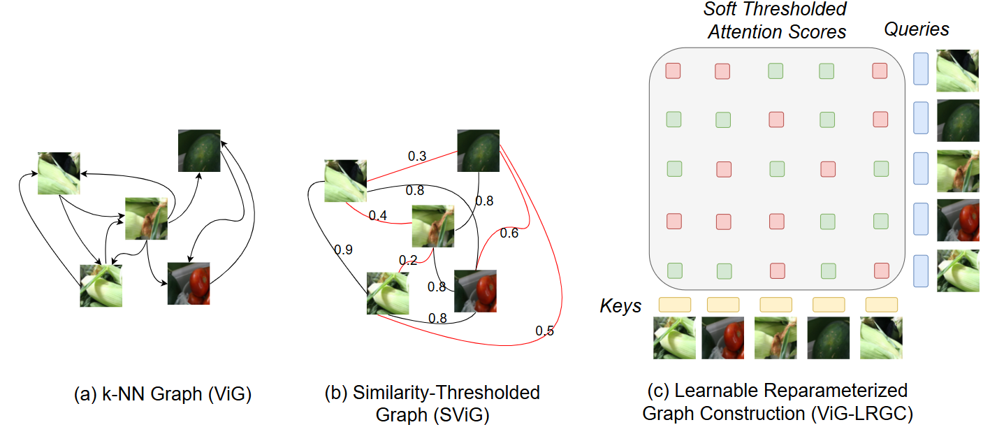
Figure 1: Graph Construction methodologies in ViG, SViG and ViG-LRGC. (a) ViG uses k-NN graph construction. In this example, k=2, thus each node has two incoming edges. (b) SViG uses similarity-thresholded graph construction. The example shows hypothetical similarity scores on edges (ingoring self-edges), with a cut-off threshold of 0.7. (c)ViG-LRGC (ours) uses Learnable Reparameterized Graph Construction (LRGC). This example shows the calculation of key and query values of all nodes, followed by the attention score calculation. In this figure, red squares are the attention scores that are below the learnable threshold $\tau$ of that layer, whereas green squares represent attention scores are higher than the learnable threshold. In other words, green squares represent selected edges and red squares represent non-selected edges.

2 Related Work

In the literature, there are two general directions of improvement to Vision Graph Neural Networks (ViG) (Han et al., 2022), which are: performing an architectural search to find the best possible GNN architecture and using alternative graph construction methodologies. The architectural search task is related to finding the best Pyramid or hybrid GNN-CNN architecture, which we leave for future work. This section is going to focus mainly on the graph construction methodologies in the literature.

ViHGNN (Han et al., 2023) introduced the concept of using a hyper-graph in GNN Vision models. A hyper-graph is a set of overlapping clusters of nodes. The clustering method they used was Fuzzy C-Means, which was an expensive operation to perform. After a hyper-graph is constructed, the there is an aggregation operation from all nodes in a cluster to a virtual super node, then another message passing operation back to the nodes in the cluster.

There was another proposition in the literature to use axial graph construction, which was used by MobileViG (Munir et al., 2023), MobileViGv2 (Avery et al., 2024) and GreedyViG (Munir et al., 2024). Axial Graph construction means that the receptive field of any patch is the set of patches on its row or column exclusively. MobileViG(Munir et al., 2023) presented Dialted Axial Graph Construction, where an edge was constructed with every other patch on the axes. The major issue with this approach was aggregating noise from irrelevant neighbors. To solve this issue, GreedyViG(Munir et al., 2024) limited the receptive field of each node to nodes on the dilated axes with a Euclidean distance that is smaller than an estimate for $\mu-\sigma$. This filters our non-important neighbors for each node; however, important neighbors that are not on the dilated axes are dropped. Similar to GreedyViG, MobileViGv2 (Avery et al., 2024) used k-NN graph construction on the dilated axes, where each node would pick the most similar k nodes on the dilated axes as neighbors. There is a significant drawback to this method, which is the fact that, similar to vanilla k-NN, each node picks the same number of neighbors. This would entail aggregating from irrelevant neighbors and dropping important neighbors.

To be able to have a more flexible graph representation, SViG (Elsharkawi et al., 2025) proposed similarity thresholded graph construction. Similarity-thresholded graph construction assumed that the edge similarity scores followed a normal distribution. Then, a fixed threshold would be used, such that the edges with a normalized similarity score above that threshold will be selected. SViG also used a decreasing-threshold framework to avoid tuning each threshold in every layer independently. This approach, while efficient, makes an assumption that nodes can only attend to the most similar nodes, which might not always be the case. In addition, the decreasing threshold framework adds two hyper-parameters to the model, which need a grid search to find the best possible combination.

Apart from image classification on ImageNet-1k, Super Resolution (SR) was another task that was solved using GNN models. SR is the task where a low-resolution image is converted to a higher resolution image. The first attempt to tackle this problem with ViG-based models was Image Processing GNNs (IPG) (Tian et al., 2024). IPG introduces the concept of a local and a global neighborhood of a patch, where the local neighborhood represents the eight patches surrounding a patch and the global neighborhood represents the dilated grid of the patch grid. Each patch is downsampled, then upsampled again and the level of detail retained represents the patch importance, which is the then used to pick a k value for that patch. Then, each patch selects the k-NN from the local and global neighborhood, where each patch has its unique value for k. This approach has many disadvantages, which include the limited receptive fields of a node, the expensive downsampling and upsampling operation and finally, the fact that this graph construction method is tailored for SR.

In contrast to graph construction in ViG-based models, Vision Transformers (ViT) (Dosovitskiy et al., 2021) performed self-attention between all tokens in a sequence and thus constructed a fully connected graph. Some variations of ViT proposed other methods for graph construction between tokens in a sequence. For example, Swin Transformers (Liu et al., 2021) proposed the use of attention only within a predefined window, such that the size and aspect ratio of the window could change in different layers. Likewise, Shuffle Transformers Huang et al. (2021) proposed performing self-attention within a predefined window, then shuffling the patches across different windows in following layers.

In our work, we propose a learnable method for graph construction that does not limit the receptive field of a node and can adapt the thresholds based on the data, instead of being fixed. We also replace similarity scores with learnable attention scores that can better represent the relationship between nodes.

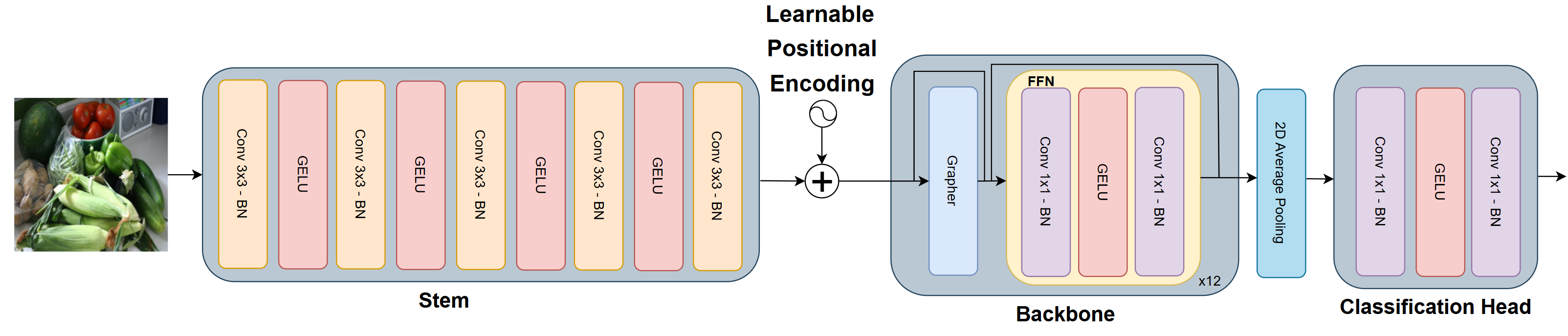
Figure 2: ViG-LRGC Model Architecture. The model has three main parts: a stem, a backbone and a classification head. The Stem is a CNN that acts as a feature extractor. That would be followed by adding learnable positional encoding. Each $1\times 1\times D$ vector in the feature map represents a node in the graph. The next part of the model shows the backbone. The backbone is a sequence of 12 Grapher and FFN modules. Grapher modules are illustrated in more detail in Figure 4. After applying 2D Average pooling to the output of the backbone, the classification head is composed of two fully connected layers that outputs 1000 classification scores.

3 Methodology

This section first presents the mathematical notation. Then, the overall architecture of the ViG-LRGC will be presented. Finally, the Learnable Reparameterized Graph Construction will be presented.

3.1 Notation

The representation of an image is $I\in\mathbb{R}^{H\times W\times 3}$, such that $H$ is the height of the image and $W$ is the width of the image. An image is represented with a graph $G=(V,E)$, where $V$ is the set of vertices in graph $G$ and $E$ is the set of edges connecting these vertices. An directed edge from node $v_{i}$ to node $v_{j}$ is denoted by $e_{i,j}\in E$. The number of nodes in an image (or graph) is $N=|V|$. There are $L_{G}$ Grapher modules in the model, where each of them is denoted by $l$, such that $1\leq l\leq L_{G}$. For each grapher module, the learnable threshold parameter is represented by $\tau_{l}$. In a Grapher module $l$, the feature vectors representing nodes of an image are denoted by $X^{l}=[x_{1}^{l},x_{2}^{l},x_{3}^{l},...,x_{N}^{l}]$, where a node $v_{i}$ in Grapher layer $l$ would be represented by a feature vector $x_{i}^{l}\in\mathbb{R}^{D}$, such that the embedding dimension of any node in any layer is $D$. For each pair of nodes $v_{i}$ and $v_{j}$ (or edge $e_{i,j}$), the attention score of these two nodes is $\alpha_{i,j}$.

3.2 Overall ViG-LRGC Architecture

ViG-LRGC architecture is adopted from ViG-Ti (Han et al., 2022). The reason for the adoption of this model architecture is to have a fair comparison with other graph construction methodologies. The model is composed of a feature extractor (called a Stem), a backbone, and finally a classification head. The overall architecture of the model is shown in Figure 2.

The feature extractor is a shallow Convolutional Neural network (CNN). There are five CNN layers in the feature extractor, where the size of the output feature map is $\frac{H}{16}\times\frac{W}{16}\times D$. This is equivalent to $\frac{H}{16}\times\frac{W}{16}$ nodes with dimensions $1\times 1\times D$ each. It is important to note that each node represents a patch of size $19\times 19\times 3$ in the input image. For each node, learnable positional embeddings of dimensions $1\times 1\times D$ are added to preserve the positional information of each node.

The backbone is the main part of the model and is composed of a series of 12 sets of Grapher and FFN modules. A Grapher module is the type of GNN layer used. The architecture of the Grapher module will be explained in detail in Section 3.3.2. The Feed Forward Network(FFN) module is a two-layer module that is there to increase the feature diversity and overcome oversmoothing. The FFN module is as follows:

$$Y=GELU(XW_{1})W_{2}+X$$ (1)

where $W_{1}$ and $W_{2}$ are learnable linear layers, $X$ is the output of the GNN and $Y\in\mathbb{R}^{N\times D}$ is the input to the next GNN layer.

The backbone is followed by a 2D Average Pooling layer, which performs feature-wise averaging across all $N$ nodes in the graph. The output of the 2D Average Pooling layer is $1\times 1\times D$, which represents the whole image. This is followed by a classification head, which is composed of two fully connected layers. Since the problem under consideration is image classification, the output of the classification head is 1000 scores corresponding to the classes of ImageNet-1k.

For ViG-LRGC, the embedding dimension $D=192$, which means that the feature vector of every node in any layer $x_{i}^{l}\in\mathbb{R}^{192}$. The input size is $224\times 224\times 3$, thus the dimension of the output feature map after the stem module is $14\times 14$, which means that a graph of an image has $196$ nodes in any layer (since we are using an isotropic architecture).

3.3 Learnable Reparameterized Graph Construction

This section will first present the graph construction methodology; then the updated Grapher module architecture will be presented. Finally, a brief overview of the implementation will be provided.

3.3.1 Graph Construction Methodology

The main motivation of the Learnable Reparameterized Graph Construction (LRGC) methodology is to have a differentiable hyper-parameter-free method for edge selection. Another motivation is to overcome the drawbacks in SViG (Elsharkawi et al., 2025); which are using similarity scores to select edges and the need for a hyper-parameter search to select the optimal threshold for each layer. We call the block that selects the edges an LRGC block. We assume that the LRGC block selects edges from a fully connected graph. Thus, we iterate over all possible (or candidate) edges in a fully connected graph. The purpose of the LRGC block is to assign a nonzero attention score to selected edges and a zero attention score for non-selected edges.

LRGC is based on concepts of Self-Attention in Vision Transformers (ViT) (Dosovitskiy et al., 2021) and Soft Threshold Reparameterization (STR) (Kusupati et al., 2020b). Figure 3 shows the LRGC methodology. In that figure, a candidate edge from node $v_{i}$ to node $v_{j}$ is shown. In addition, the learnable threshold $\tau$ is shown as an input to the block. This procedure is performed for all possible edges in the graph. It is important to note that each grapher module has its own $\tau$.

Similar to the self-attention of visual tokens in Vision Transformers (Dosovitskiy et al., 2021), we calculate the attention score between every pair of nodes. For nodes $v_{i}$ and $v_{j}$, the attention score $\alpha^{{}^{\prime}}_{i,j}$ is calculated as follows:

$$\begin{split}&key(v_{i})=W_{key}h_{i}\\ &query(v_{j})=W_{query}h_{j}\\ &\alpha^{{}^{\prime}}_{i,j}=key(v_{i})\cdot query(v_{j})\\ \end{split}$$ (2)

where $W_{key}$ and $W_{query}$ are learnable linear layers. A key and a query of a node are linear projections of the hidden representation of that node. The dot product of the key of node $v_{i}$ and the query of node $v_{j}$ represents a lookup in a query table or the importance of a node relative to another.

We borrow the concept of soft threshold reparameterization from STR (Kusupati et al., 2020b). We use the attention score $\alpha^{{}^{\prime}}_{i,j}$ calculated in Equation 2 as follows:

$$\begin{split}&\alpha^{{}^{\prime\prime}}_{i,j}=ReLU(\sigma(\alpha^{{}^{\prime}}_{i,j})-\sigma(\tau))\\ &\alpha_{i,j}=\tanh(\alpha^{{}^{\prime\prime}}_{i,j})\end{split}$$ (3)

We subtract the sigmoid of the learnable threshold $\tau$ from the sigmoid of $\alpha^{{}^{\prime}}_{i,j}$ and apply a $ReLU$ to the difference. The intuition is to have a zero score when $\alpha^{{}^{\prime}}_{i,j}\leq\tau$ and a nonzero score otherwise. The purpose of using sigmoids with the threshold $\tau$ and $\alpha^{{}^{\prime}}_{i,j}$ is to make training numerically stable, since the difference will always be smaller than 1. Finally, $\tanh$ is applied as a scaling function that preserves the value of zero attention scores.

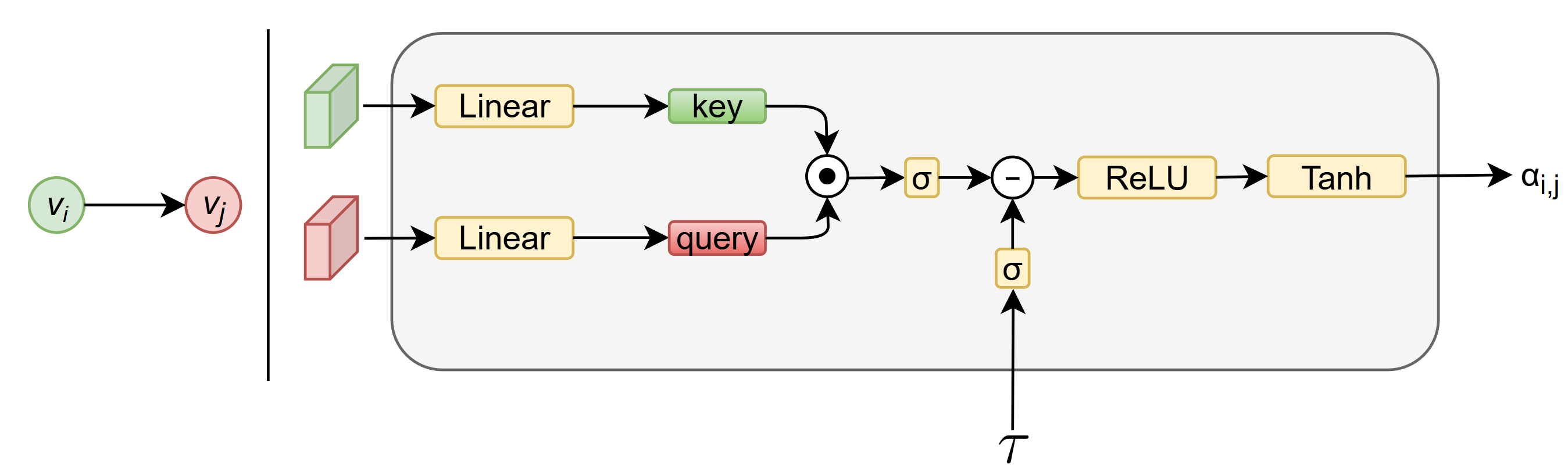
Figure 3: Learnable Reparameterized Graph Construction (LRGC) Block. This Figure corresponds to Equation 4 Left: There is an edge from node $v_{i}$ to $v_{j}$ under consideration. Right: Nodes $v_{j}$ and $v_{i}$ are fed through two different linear layers to get their query and key respectively. We subtract the sigmoid of the learnable threshold $\tau$ from the sigmoid of the dot product of the key of node $v_{i}$ and query of node $v_{j}$. This subtraction is then passed through a ReLU to filter out edges with attention scores below $\tau$. The attention score is passed through a $\tanh$ to get $\alpha_{i,j}$, which is then used in the updated Grapher module (shown in Figure 4).

Putting together Equations 2 and 3, we calculate the attention scores as follows:

$$\begin{split}&\alpha_{i,j}=\tanh(ReLU(\sigma(W_{key}h_{i}\cdot W_{query}h_{j})-\sigma(\tau)))\\ \end{split}$$ (4)

It is important to mention that the purpose of this methodology is to prune non-needed edges. Thus $\tau$ should be initialized with a low value to be able to have a fully connected graph during the first optimization step, and then allow the model to prune edges that are not important. We choose to initialize $\tau$ at -1 for all layers. We show empirically in Figure 5 that this initialization value allows the graph to be fully connected in the first optimization step.

3.3.2 Updated Grapher Module

We adopt the Grapher module architecture from ViG-Ti (Han et al., 2022) with only one modification: we add the learned attention score to the Max-Relative Graph Convolution. The updated Grapher module can be described via the following set of equations:

$$\begin{split}&{x_{j}}^{{}^{\prime}}={x_{j}}^{l}W_{in}\\ &{x_{j}}^{{}^{\prime\prime}}=\max(\alpha_{i,j}({{x_{i}}^{{}^{\prime}}-{x_{j}}^{{}^{\prime}})|v_{i}\in\textit{Neighborhood}({v_{j}})})\\ &{x_{j}}^{{}^{\prime\prime\prime}}=GELU([{x_{j}}^{{}^{\prime}},{x_{j}}^{{}^{\prime\prime}}]W_{update})W_{out}\\ &{x_{j}}^{l+1}={x_{j}}^{{}^{\prime\prime\prime}}+x_{j}^{l}\\ \end{split}$$ (5)

where $W_{in}$, $W_{update}$ and $W_{out}$ are learnable linear layers. In addition, $W_{update}$ is a multi-head update layer with 4 update heads. $\alpha_{i,j}$ is the attention score that was obtained from Equation 4. $x_{j}^{{}^{\prime}}$, $x_{j}^{{}^{\prime\prime}}$ and $x_{j}^{{}^{\prime\prime\prime}}$ are intermediate representations of node $v_{j}$ in the Grapher module.

Figure 4 shows the updated Grapher module. In that figure, $v_{i}$ and $v_{k}$ are the source nodes; while $v_{j}$ is the target node. This means that there are two edges to consider: an edge from node $v_{i}$ to node $v_{j}$ and another one from node $v_{k}$ to node $v_{j}$. First, the node feature vectors are fed to a linear layer. Then, every pair of nodes is fed into the LRGC block to get an attention score for the edge being considered. That would be followed by multiplying the attention score by the subtraction of the feature vectors of the source and target nodes. This multiplication operation with $\alpha_{i,j}$ is important to allow the model to be differentiable. Then, the residuals that were multiplied by the attention scores go through a feature-wise max-pooling operation. Effectively, non-selected edges would have the residuals multiplied by zero, which means that the feature values do not affect the max-pooling operation.

This would be followed by a concatenation with the feature vector of the target node, then a Linear, a GELU (Hendrycks and Gimpel, 2016) activation function and a Linear layer. Finally, there is a residual connection with the input feature vector of the target node.

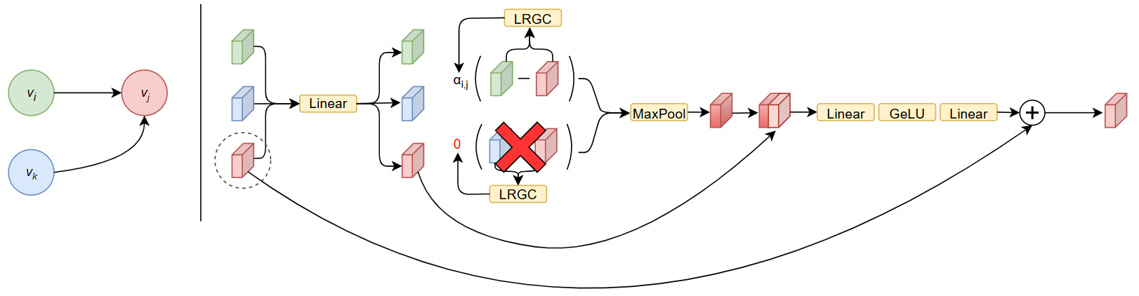
Figure 4: Updated Grapher module. This Figure corresponds to Equation 5. Left: This is a hypothetical graph with three nodes: $v_{i}$, $v_{k}$ and $v_{j}$, where there is an edge from node $v_{i}$ to node $v_{j}$ and an edge from node $v_{k}$ to node $v_{j}$. The target node is node $v_{j}$. Right: The inputs are $x_{i},x_{j}$ and $x_{k}$, which are the representations of nodes $v_{i}$, $v_{j}$ and $v_{k}$ (with the target node representation $x_{j}$ being circled). All nodes are fed through a linear layer. Then, for every edge, both nodes are fed to an LRGC module to calculate the attention scores $\alpha_{i,j}$ and $\alpha_{k,j}$. In this example, $\alpha_{k,j}=0$, which means that the edge was not selected. The residuals, which are multiplied by the attention scores $\alpha_{i,j}$ and $\alpha_{k,j}$, are fed to a Max-Pooling layer. This is followed by a concatenation with the representation of the target node, then two linear layers and a residual connection.

3.4 LRGC Implementation

We use the flexible aggregation from SViG (Elsharkawi et al., 2025) because it does not place a constraint on each node to have a specific number of neighbors in the graph. However, there is a need to start with a fully connected graph to allow the model to prune the edges in a fair manner. This means that $\tau$ is initialized with a low value and that all edges are selected during the first optimization step. This places a limitation on the computational power needed for the implementation of ViG-LRGC, which in turn affects the batch size (discussed in more detail in Section 4.2).

4 Experiments

In this section, the dataset used is described. Then, the experimental setup used for our experimentation is presented. We then compare our model with the state-of-the-art models in the literature. Finally, we perform an analysis for our ViG-LRGC model.

4.1 Dataset

We used ImageNet-1k (ImageNet ILSVRC 2012) dataset (Russakovsky et al., 2015) in our experiments. This dataset could be obtained via a license from https://www.image-net.org/download. There are 1.2 million images in the training set and 50k images in the testing set. This dataset is used for the image classification task and it has 1000 classes.

Table 1: Hyper-parameters used in the training of ViG-LRGC

Hyper-parameter Value set for ViG-LRGC Epochs 300 Optimizer AdamW (Loshchilov and Hutter, 2017) Batch size 256 Start learning rate (LR) 2e-3 Learning rate Schedule Cosine Warmup epochs 20 Weight decay 0.05 Label smoothing(Szegedy et al., 2016) 0.1 Stochastic path(Huang et al., 2016) 0.1 Repeated augment(Hoffer et al., 2020) ✓ RandAugment (Cubuk et al., 2020) ✓ Mixup prob. (Zhang et al., 2018) 0.8 Cutmix prob. (Yun et al., 2019) 1.0 Random erasing prob. (Zhong et al., 2020) 0.25 Exponential moving average 0.99996

Table 2: Comparing ViG-LRGC to GNN architectures. This table shows the results of the experiments that we ran using a batch size of 256. It can be observed that ViG-LRGC surpasses the ViG-Ti baseline by 3.8% on Top-1 Accuracy while surpassing SViG-Ti by 2.4%

Model Params (M) FLOPs (B) Top-1 Top-5 ViG-LRGC(ours) 8.1 1.5 74.3 92.3 ViG-Ti(Han et al., 2022) 7.2 1.3 70.5 89.9 SViG-Ti(Elsharkawi et al., 2025) 7.2 1.3 71.9 90.8

4.2 Experimental Setup

In our implementation, we used PyTorch 1.7.1 (Paszke et al., 2019), PyTorch Geometric (PyG) 2.3.1 (Fey and Lenssen, 2019) and PyTorch Image Models (Timm) 0.3.2 (Wightman, 2019). We use PyTorch Distributed Data Parallel (DDP) to train our model on a DGX-1 server with 8 NVIDIA V100 GPUs (with 32 GB of memory each). During training, the same batch size should be used for all optimization steps. However, due to the need to have a fully connected graph in the first optimization step (as described in Section 3.4), the effective batch size used is 256 due to computational power limitations. For a fair comparison, we use the same training hyper-parameters used for ViG (Han et al., 2022). The hyper-parameters used for training are shown in Table 1. For each reported result, we train the model from scratch on ImageNet for 300 epochs with 20 warmup epochs and 10 cooldown epochs. We resize all images to $224\times 224\times 3$. The optimizer we used was AdamW (Loshchilov and Hutter, 2017). The learning rate schedule used was a Cosine Annealing schedule with a base learning rate of $2e-3$. The data augmentation methods used were CutMix (Yun et al., 2019), MixUp (Zhang et al., 2018), RandAugment (Cubuk et al., 2020), repeated augment (Hoffer et al., 2020) and random erasing (Zhong et al., 2020). For all layers, $\tau$ is initialized with -1.

4.3 Experimental Results

In order to have a fair comparison, we focus on state-of-the-art isotropic models that have a similar number of parameters and that focus solely on graph construction. We choose to have a comparison with ViG-Ti (Han et al., 2022) baseline and SViG-Ti (Elsharkawi et al., 2025), which adopt the same model architecture as ViG-Ti.

Since we use a batch size of 256 to train ViG-LRGC, we replicate the training experiments for both ViG-Ti (Han et al., 2022) and SViG-Ti (Elsharkawi et al., 2025) with the same batch size to have a fair comparison. We present our experimental results in Table 2.

4.3.1 Effect of the batch size on the training

For the same model, we observe that using a smaller batch size yields lower results (while still using the same hyper-parameters and training setup). For ViG-Ti, using a batch size of 256 yields a Top-1 Accuracy of 70.5%, opposed to a Top-1 of 73.9% when using a batch size of 1024. Similarly, the Top-1 Accuracy of SViG-Ti, when using a batch size of 256, is 71.9%, while the Top-1 Accuracy of SViG-Ti becomes 74.6% when using a batch size of 1024.

4.3.2 Comparison to the State Of The Art

The Top-1 Accuracy of ViG-LRGC is 74.3% and the Top-5 Accuracy is 92.3%. Using the same batch size of 256, we show that our ViG-LRGC model surpasses the baseline ViG-Ti with 3.8% on Top-1 Accuracy and 2.4% on Top-5 Accuracy. Our ViG-LRGC also surpasses SViG-Ti with 2.4% on Top-1 Accuracy and 1.5% for Top-5 Accuracy. Our ViG-LRGC model outperforms the state-of-the-art GNN isotropic models, that are trained with the same hyper-parameters.

4.4 Computational Complexity of LRGC

In both ViG and SViG, the computational complexity of the graph aggregation was dominated by the calculation of the similarity matrix. The similarity score calculation computational complexity is $O(N^{2}*D)$, where $D$ is the embedding size and $N$ is the number of nodes in an image (Elsharkawi et al., 2025) Assuming that $N\approx D$, then the complexity becomes $O(N^{3})$.

For ViG-LRGC, the multiplication of a feature vector of a node by the weights of $W_{key}$ or $W_{query}$ has a computational complexity of $O(D^{2})$, since the size of both the input and output feature vectors is $1\times\ 1\times D$. To calculate the values of the keys and the queries of all $N$ nodes in an image, the complexity becomes $O(N*D^{2})$. The computational complexity of the dot product of the key and query is $O(D)$. Since we assume a fully connected graph, the calculation of all attention scores has a computational complexity of $O(D*N^{2})$ since there are $N^{2}$ edges in a fully-connected graph. If we assume that $N\approx D$, then the total complexity becomes $O(N*D^{2}+D*N^{2})\approx O(N^{3})$. Thus, the complexity of ViG-LRGC is similar to ViG-Ti and SViG-Ti. This is experimentally proven by the fact that ViG-LRGC has a FLOPs count of 1.6B, compared to 1.3B of both ViG-Ti and SViG-Ti. While the number of parameters of a ViG-LRGC model is slightly larger than that of ViG-Ti and SViG-Ti, the slight increase is justifiable due to the increase in performance.

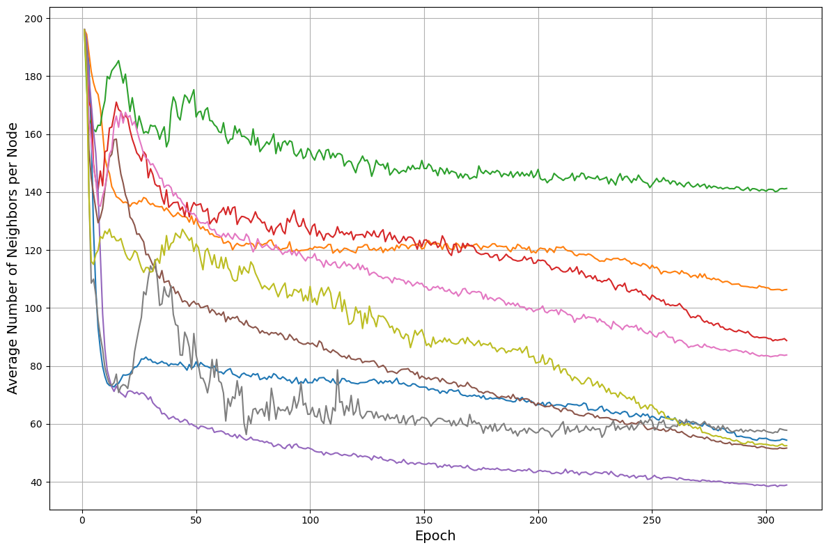
Figure 5: This figure shows the average number of neighbors per node for the training epochs. Each line represents the average number of neighbors per node for a different layer. This Figure proves the pruning power of LRGC for non-needed edges.

4.5 Empirical Proof for the Pruning Power of LRGC

To prove the pruning power of ViG-LRGC, Figure 5 shows the average number of neighbors per node for some layers. This figure shows how the average number of neighbors per node changes across the training epochs. The average number of neighbors can be seen as a reflection of the change in the threshold $\tau$ in each layer. As seen, the average number of nodes starts from the maximum possible value (196). During the first 50 epochs, the average number of nodes first decreases, then increases slightly then drops again. Starting from epoch 50, the average number of nodes decreases steadily. Each layer tunes the learnable threshold $\tau$ based on the training data. Opposed to hard-thresholding in SViG(Elsharkawi et al., 2025), the soft-thresholding allows the learning of the threshold $\tau$. This is similar to the trend of the weight pruning that is observed in STR (Kusupati et al., 2020a).

5 Conclusion

In conclusion, we present a novel method for graph construction in Vision Graph Neural Networks. Our Learnable Reparameterized Graph Construction (LRGC) methodology proposes a powerful alternative for the similarity score calculation through the learnable attention scores. Moreover, LRGC presents learnable thresholding by utilizing the reparameterization trick to learn the threshold for each layer; thus, removing the need for a grid search over hyper-parameters. We prove that LRGC has a great pruning power for non-needed edges. Our methodology is superior to the state-of-the-art GNN models with similar sizes, with a minimal increase in FLOPs. We hope that this work inspires future work on Pyramid or GNN-CNN hybrid models that use LRGC as a learnable method for graph construction.

References

- Russakovsky et al. [2015] Olga Russakovsky, Jia Deng, Hao Su, Jonathan Krause, Sanjeev Satheesh, Sean Ma, Zhiheng Huang, Andrej Karpathy, Aditya Khosla, Michael Bernstein, et al. Imagenet large scale visual recognition challenge. International Journal of Computer Vision, 115(3):211–252, 2015.
- Ridnik et al. [2021] Tal Ridnik, Emanuel Ben-Baruch, Asaf Noy, and Lihi Zelnik-Manor. Imagenet-21k pretraining for the masses, 2021. URL https://arxiv.org/abs/2104.10972.
- Sun et al. [2017] Chen Sun, Abhinav Shrivastava, Saurabh Singh, and Abhinav Gupta. Revisiting unreasonable effectiveness of data in deep learning era, 2017. URL https://arxiv.org/abs/1707.02968.
- Lecun et al. [1998] Y. Lecun, L. Bottou, Y. Bengio, and P. Haffner. Gradient-based learning applied to document recognition. Proceedings of the IEEE, 86(11):2278–2324, 1998. doi:10.1109/5.726791.
- Dosovitskiy et al. [2021] Alexey Dosovitskiy, Lucas Beyer, Alexander Kolesnikov, Dirk Weissenborn, Xiaohua Zhai, Thomas Unterthiner, Mostafa Dehghani, Matthias Minderer, Georg Heigold, Sylvain Gelly, Jakob Uszkoreit, and Neil Houlsby. An image is worth 16x16 words: Transformers for image recognition at scale. ICLR, 2021.
- Tolstikhin et al. [2021] Ilya Tolstikhin, Neil Houlsby, Alexander Kolesnikov, Lucas Beyer, Xiaohua Zhai, Thomas Unterthiner, Jessica Yung, Andreas Steiner, Daniel Keysers, Jakob Uszkoreit, Mario Lucic, and Alexey Dosovitskiy. Mlp-mixer: An all-mlp architecture for vision. arXiv preprint arXiv:2105.01601, 2021.
- Han et al. [2022] Kai Han, Yunhe Wang, Jianyuan Guo, Yehui Tang, and Enhua Wu. Vision gnn: An image is worth graph of nodes. In NeurIPS, 2022.
- Krizhevsky et al. [2012] Alex Krizhevsky, Ilya Sutskever, and Geoffrey E Hinton. Imagenet classification with deep convolutional neural networks. In F. Pereira, C.J. Burges, L. Bottou, and K.Q. Weinberger, editors, Advances in Neural Information Processing Systems, volume 25. Curran Associates, Inc., 2012. URL https://proceedings.neurips.cc/paper_files/paper/2012/file/c399862d3b9d6b76c8436e924a68c45b-Paper.pdf.
- Vaswani et al. [2023] Ashish Vaswani, Noam Shazeer, Niki Parmar, Jakob Uszkoreit, Llion Jones, Aidan N. Gomez, Lukasz Kaiser, and Illia Polosukhin. Attention is all you need, 2023. URL https://arxiv.org/abs/1706.03762.
- Sen et al. [2008] Prithviraj Sen, Galileo Namata, Mustafa Bilgic, Lise Getoor, Brian Galligher, and Tina Eliassi-Rad. Collective classification in network data. AI magazine, 29(3):93–93, 2008.
- Hamilton et al. [2017] William L Hamilton, Rex Ying, and Jure Leskovec. Inductive representation learning on large graphs. In NIPS, pages 1025–1035, 2017.
- Wale et al. [2008] Nikil Wale, Ian A Watson, and George Karypis. Comparison of descriptor spaces for chemical compound retrieval and classification. Knowledge and Information Systems, 14(3):347–375, 2008.
- Wang et al. [2018] Yue Wang, Yongbin Sun, Ziwei Liu, Sanjay E. Sarma, Michael M. Bronstein, and Justin M. Solomon. Dynamic graph CNN for learning on point clouds. CoRR, abs/1801.07829, 2018. URL http://arxiv.org/abs/1801.07829.
- Li et al. [2019] Guohao Li, Matthias Müller, Ali K. Thabet, and Bernard Ghanem. Can gcns go as deep as cnns? CoRR, abs/1904.03751, 2019. URL http://arxiv.org/abs/1904.03751.
- Elsharkawi et al. [2025] Ismael Elsharkawi, Hossam Sharara, and Ahmed Rafea. Svig: A similarity-thresholded approach for vision graph neural networks. IEEE Access, 13:19379–19387, 2025. doi:10.1109/ACCESS.2025.3531691.
- Kusupati et al. [2020a] Aditya Kusupati, Vivek Ramanujan, Raghav Somani, Mitchell Wortsman, Prateek Jain, Sham Kakade, and Ali Farhadi. Soft threshold weight reparameterization for learnable sparsity, 2020a. URL https://arxiv.org/abs/2002.03231.
- Kingma et al. [2015] Diederik P. Kingma, Tim Salimans, and Max Welling. Variational dropout and the local reparameterization trick, 2015. URL https://arxiv.org/abs/1506.02557.
- Han et al. [2023] Yan Han, Peihao Wang, Souvik Kundu, Ying Ding, and Zhangyang Wang. Vision HGNN: an image is more than a graph of nodes. In IEEE/CVF International Conference on Computer Vision, ICCV 2023, Paris, France, October 1-6, 2023, pages 19821–19831. IEEE, 2023. doi:10.1109/ICCV51070.2023.01820. URL https://doi.org/10.1109/ICCV51070.2023.01820.
- Munir et al. [2023] Mustafa Munir, William Avery, and Radu Marculescu. Mobilevig: Graph-based sparse attention for mobile vision applications. In IEEE/CVF Conference on Computer Vision and Pattern Recognition, CVPR 2023 - Workshops, Vancouver, BC, Canada, June 17-24, 2023, pages 2211–2219. IEEE, 2023. doi:10.1109/CVPRW59228.2023.00215. URL https://doi.org/10.1109/CVPRW59228.2023.00215.
- Avery et al. [2024] William Avery, Mustafa Munir, and Radu Marculescu. Scaling graph convolutions for mobile vision. In Proceedings of the IEEE/CVF Conference on Computer Vision and Pattern Recognition (CVPR) Workshops, pages 5857–5865, 2024.
- Munir et al. [2024] Mustafa Munir, William Avery, Md Mostafijur Rahman, and Radu Marculescu. Greedyvig: Dynamic axial graph construction for efficient vision gnns. In Proceedings of the IEEE/CVF Conference on Computer Vision and Pattern Recognition (CVPR), 2024.
- Tian et al. [2024] Yuchuan Tian, Hanting Chen, Chao Xu, and Yunhe Wang. Image processing gnn: Breaking rigidity in super-resolution. In Proceedings of the IEEE/CVF Conference on Computer Vision and Pattern Recognition (CVPR), pages 24108–24117, 2024.
- Liu et al. [2021] Ze Liu, Yutong Lin, Yue Cao, Han Hu, Yixuan Wei, Zheng Zhang, Stephen Lin, and Baining Guo. Swin transformer: Hierarchical vision transformer using shifted windows. In ICCV, 2021.
- Huang et al. [2021] Zilong Huang, Youcheng Ben, Guozhong Luo, Pei Cheng, Gang Yu, and Bin Fu. Shuffle transformer: Rethinking spatial shuffle for vision transformer. arXiv:2106.03650, 2021.
- Kusupati et al. [2020b] Aditya Kusupati, Vivek Ramanujan, Raghav Somani, Mitchell Wortsman, Prateek Jain, Sham M. Kakade, and Ali Farhadi. Soft threshold weight reparameterization for learnable sparsity. CoRR, abs/2002.03231, 2020b. URL https://arxiv.org/abs/2002.03231.
- Hendrycks and Gimpel [2016] Dan Hendrycks and Kevin Gimpel. Gaussian error linear units (gelus). arXiv preprint arXiv:1606.08415, 2016.
- Loshchilov and Hutter [2017] Ilya Loshchilov and Frank Hutter. Decoupled weight decay regularization. arXiv preprint arXiv:1711.05101, 2017.
- Szegedy et al. [2016] Christian Szegedy, Vincent Vanhoucke, Sergey Ioffe, Jon Shlens, and Zbigniew Wojna. Rethinking the inception architecture for computer vision. In IEEE Conference on Computer Vision and Pattern Recognition, pages 2818–2826, 2016.
- Huang et al. [2016] Gao Huang, Yu Sun, Zhuang Liu, Daniel Sedra, and Kilian Q Weinberger. Deep networks with stochastic depth. In ECCV, pages 646–661. Springer, 2016.
- Hoffer et al. [2020] Elad Hoffer, Tal Ben-Nun, Itay Hubara, Niv Giladi, Torsten Hoefler, and Daniel Soudry. Augment your batch: Improving generalization through instance repetition. In CVPR, 2020.
- Cubuk et al. [2020] Ekin D Cubuk, Barret Zoph, Jonathon Shlens, and Quoc V Le. Randaugment: Practical automated data augmentation with a reduced search space. In CVPR Workshops, 2020.
- Zhang et al. [2018] Hongyi Zhang, Moustapha Cisse, Yann N Dauphin, and David Lopez-Paz. mixup: Beyond empirical risk minimization. In ICLR, 2018.
- Yun et al. [2019] Sangdoo Yun, Dongyoon Han, Seong Joon Oh, Sanghyuk Chun, Junsuk Choe, and Youngjoon Yoo. Cutmix: Regularization strategy to train strong classifiers with localizable features. In ICCV, 2019.
- Zhong et al. [2020] Zhun Zhong, Liang Zheng, Guoliang Kang, Shaozi Li, and Yi Yang. Random erasing data augmentation. In AAAI, volume 34, pages 13001–13008, 2020.
- Paszke et al. [2019] Adam Paszke, Sam Gross, Francisco Massa, Adam Lerer, James Bradbury, Gregory Chanan, Trevor Killeen, Zeming Lin, Natalia Gimelshein, Luca Antiga, et al. Pytorch: An imperative style, high-performance deep learning library. NeurIPS, 2019.
- Fey and Lenssen [2019] Matthias Fey and Jan E. Lenssen. Fast graph representation learning with PyTorch Geometric. In ICLR Workshop on Representation Learning on Graphs and Manifolds, 2019.
- Wightman [2019] Ross Wightman. Pytorch image models. https://github.com/rwightman/pytorch-image-models, 2019.