Graph-based Clustering Revisited:
A Relaxation of Kernel $k$-Means Perspective

Abstract

The well-known graph-based clustering methods, including spectral clustering, symmetric non-negative matrix factorization, and doubly stochastic normalization, can be viewed as relaxations of the kernel $k$-means approach. However, we posit that these methods excessively relax their inherent low-rank, nonnegative, doubly stochastic, and orthonormal constraints to ensure numerical feasibility, potentially limiting their clustering efficacy. In this paper, guided by our theoretical analyses, we propose Low-Rank Doubly stochastic clustering (LoRD), a model that only relaxes the orthonormal constraint to derive a probabilistic clustering results. Furthermore, we theoretically establish the equivalence between orthogonality and block diagonality under the doubly stochastic constraint. By integrating Block diagonal regularization into LoRD, expressed as the maximization of the Frobenius norm, we propose B-LoRD, which further enhances the clustering performance. To ensure numerical solvability, we transform the non-convex doubly stochastic constraint into a linear convex constraint through the introduction of a class probability parameter. We further theoretically demonstrate the gradient Lipschitz continuity of our LoRD and B-LoRD enables the proposal of a globally convergent projected gradient descent algorithm for their optimization. Extensive experiments validate the effectiveness of our approaches. The code is publicly available at https://github.com/lwl-learning/LoRD.

Keywords: Graph-based clustering, low-rank, kerne $k$-means, block diagonal, doubly stochastic

1 Introduction

Graph-based clustering (Schaeffer, 2007; Berahmand et al., 2025; Xue et al., 2024; Kang et al., 2021; Wu et al., 2022) stands as a foundational technique in data mining and machine learning, aiming to partition data points based on similarity among samples. In this study, we approach graph-based clustering through the lens of kernel $k$-means.

1.1 Kernel $k$-means and its Variants

Let $\{x_{1},\dots,x_{n}\}$ be $n$ data points to be grouped into $k$ clusters $G_{1},\dots,G_{k}$, and $S_{ij}=\kappa(x_{i},x_{j})$ be a symmetric similarity matrix defined by a kernel function $\kappa(x_{i},x_{j})$, e.g., $\kappa(x_{i},x_{j})=\exp(-\|x_{i}-x_{j}\|^{2}/\sigma^{2})$ for the Gaussian kernel. Kernel $k$-means (Dhillon et al., 2004) seeks to maximize intra-class similarity by partitioning data into clusters $G_{1},\dots,G_{k}$, as expressed by

$$\max_{G_{1},\dots,G_{k}}\sum_{r=1}^{k}\frac{1}{n_{r}}\sum_{x_{i},x_{j}\in G_{r}}S_{ij},$$ (1)

where $n_{r}=|G_{r}|$ represents the size of $G_{r}$. To transform Eq. (1) into matrix form, we introduce the class assignment matrix $V\in\mathbb{R}^{n\times k}$ with $V_{ij}=1/\sqrt{n_{j}}$ if $x_{i}\in G_{j}$ and zero otherwise. Notably, the definition of $V$ aligns with constraints $V\geq 0,VV^{T}1_{n}=1_{n},V^{T}V=I_{k}$, where $1_{n}$ is an $n$-dimensional vector of ones, $I_{k}$ is the identity matrix of size $k$, $V\geq 0$ means $\forall i,j,V_{ij}\geq 0$. Consequently, Eq. (1) can be equivalently expressed as:

$$\max_{V\geq 0}\mathrm{Tr}(V^{T}SV),\;\text{s.t.}\;VV^{T}1_{n}=1_{n},V^{T}V=I_{k}.$$ (2)

Another equivalent form of Eq. (2) is written as (Ding et al., 2005):

$$\min_{V\geq 0}\|S-VV^{T}\|_{F}^{2},\;\text{s.t.}\;VV^{T}1_{n}=1_{n},V^{T}V=I_{k},$$ (3)

where $\|\cdot\|_{F}$ denotes the Frobenius norm. In Eq. (2) and Eq. (3), the low-rank constraint $V\in\mathbb{R}^{n\times k}$ and the nonnegative constraint $V\geq 0$ make $V$ class-indicative. Specifically, $\hat{y_{i}}=\arg\max_{j}V_{ij}$ can be regarded as an estimation of the cluster index of $x_{i}$. Meanwhile, the doubly stochastic constraint $VV^{T}1_{n}=1_{n}$ enables $V_{ij}$ to express the probability that $x_{i}$ belongs to cluster $G_{j}$, as will be discussed in Theorem 2. Moreover, the orthonormal constraint $V^{T}V=I_{k}$ makes $V$ more discriminatory. We will demonstrate in Theorem 4 that the orthogonality of $V$ is closely related to the block diagonality (Lu et al., 2018) of $VV^{T}$.

However, kernel $k$-means poses an NP-hard problem (Aloise et al., 2009). By relaxing the constraints in Eq. (2) to make it numerically tractable, a series of classic graph-based clustering methods are derived as follows.

Figure 1: Schematic diagram of graph-based clustering methods. \raisebox{-1pt} {1}⃝: The models in Eq. (2) and Eq. (3) are equivalent. \raisebox{-1pt} {2}⃝: SC, SymNMF and DSN are overly relaxed kernel $k$-means. \raisebox{-1pt} {3}⃝: The model in Eq. (12) only relaxes the least important orthonormal constraint $V^{T}V=I_{k}$. \raisebox{-1pt} {4}⃝: The non-convex constraint $VV^{T}1_{n}=1$ can be reduced to a convex constraint $V^{T}1_{n}=\mu,V\mu=1_{n}/n$ by incorporating the class probability parameter $\mu$ (Theorems 1 and 2), making our LoRD numerically solvable and interpretable in terms of probability. \raisebox{-1pt} {5}⃝: The $k$-block diagonality of $VV^{T}$ can be adjusted by tuning $\gamma\in[-\lambda_{\max}(S),-\lambda_{\min}(S)]$ in B-LoRD. \raisebox{-1pt} {6}⃝: kernel $k$-means, SC, SymNMF, and DSC can be seen as a relaxation or approximation of our LoRD and B-LoRD.

1) Spectral clustering (SC) (Von Luxburg, 2007). SC only retains the orthonormal constraint in Eq. (2), i.e.,

$$\max_{V^{T}V=I_{k}}\mathrm{Tr}(V^{T}SV).$$ (4)

The optimum of Eq. (4) is given by the eigenvectors of $S$ corresponding to the largest $k$ eigenvalues. However, since the nonnegative constraint $V\geq 0$ is relaxed, $V$ cannot directly provide the clustering result. Thus, SC requires post-processing to obtain the clustering result, such as performing $k$-means on $V$.

2) Symmetric non-negative matrix factorization (SymNMF) (Kuang et al., 2012, 2015). In contrast to SC, SymNMF only retains the nonnegative constraint in Eq. (3), i.e.:

$$\min_{V\geq 0}\|S-VV^{T}\|_{F}^{2}.$$ (5)

SymNMF can obtain clustering results without post-processing. However, the probabilistic interpretability and discriminability are compromised because the doubly stochastic constraint is relaxed.

3) Doubly stochastic normalization (DSN) (Zass and Shashua, 2005, 2006). DSN relaxes the orthonormal constraint $V^{T}V=I_{k}$ and the low-rank constraint by parameterizing $Z=VV^{T}$ in Eq. (3) to solve the following convex problem:

$$\min_{Z\geq 0}\|S-Z\|_{F}^{2},\;\text{s.t.}\;Z=Z^{T},Z1_{n}=1_{n}.$$ (6)

The probabilistic interpretability of $Z$ is analyzed in (Zass and Shashua, 2005). However, the low-rank structure in $Z$ is relaxed, resulting in the need for post-processing to extract the clustering result from $Z$, such as performing SC on it.

In conclusion, SC, SymNMF, and DSN are essentially relaxations of the kernel $k$-means, and their relationships are schematically drawn in Fig. 1. However, the necessity for relaxation to ensure numerical tractability may limit the overall clustering performance of these methods.

Among the constraints in Eq. (2) and Eq. (3), the orthonormal constraint $V^{T}V=I_{k}$ and the doubly stochastic constraint $VV^{T}1_{n}=1_{n}$ are the most difficult to handle in optimization. From the perspective of clustering, the orthonormal constraint is considered the least crucial (Zass and Shashua, 2005, 2006), because removing $V^{T}V=I_{k}$ only transforms the original problem from hard clustering to soft clustering. In this paper, to handle the doubly stochastic constraint, we prove in Theorem 1 and Theorem 2 that $VV^{T}1_{n}=1_{n}$ can be reduced to a linear convex constraint $V^{T}1_{n}=\mu,V\mu=1_{n}/n$, where $\mu$ is a user-specified parameter associated with class prior probability. This observation enables the optimization problem to be solved efficiently. Moreover, we establish the connection between the orthogonality of $V$ and the block diagonality of $VV^{T}$ in Theorem 4, so that the relaxed orthonormal constraint can be remedied by adding a block diagonal regularization of $VV^{T}$, as introduced in the subsequent subsection.

1.2 Block Diagonal Structure

An ideal clustering structure for a similarity matrix $S\in\mathbb{R}^{n\times n}$ with $n$ data points is one that has exactly $k$ connected components, where $k$ is the number of clusters, and each connected component corresponds to a cluster. Such an $S$ can be expressed as a $k$-block diagonal matrix (Feng et al., 2014; Lu et al., 2018) as follows:

$$S=\begin{bmatrix}S_{1}&0&\cdots&0\\ 0&S_{2}&\cdots&0\\ \vdots&\vdots&\ddots&\vdots\\ 0&0&\cdots&S_{k}\\ \end{bmatrix},\;\text{where}\;S_{i}\in\mathbb{R}^{n_{i}\times n_{i}}.$$ (7)

According to the spectral graph theorem (Von Luxburg, 2007), the number of connected components of $S$ is equal to the multiplicity $k$ of the eigenvalue $0$ of the Laplacian matrix $L_{S}=\mathrm{Diag}(S1_{n})-S$, where $\mathrm{Diag}(z)$ is a diagonal matrix with $z$ as its diagonal elements. Building on this insight, the $k$-block diagonal structure of $S$ can be achieved by constraining $\mathrm{rank}(L_{S})=n-k$ (Wang et al., 2016). However, the constraint is difficult to handle directly in optimization. The most common approach is to relax it to a regularization $\|S\|_{\hbox to6.82pt{\vbox to7.26pt{\text{[drawing]}}}}$ using Ky Fan’s theorem (Wang et al., 2016; Xie et al., 2017; Nie et al., 2014), i.e.,

$$\|S\|_{\hbox to6.82pt{\vbox to7.26pt{\text{[drawing]}}}}:=\sum_{i=n-k+1}^{n}\lambda_{i}(L_{S})=\min_{\begin{subarray}{c}0\preceq W\preceq I_{n}\\ \mathrm{Tr}(W)=k\end{subarray}}\langle L_{S},W\rangle, k$$ (8)

where $\lambda_{i}(L_{S})$ is the $i$-th largest eigenvalue of $L_{S}$, and $0\preceq W\preceq I_{n}$ means that $0\leq\lambda_{\min}(W)\leq\lambda_{\max}(W)\leq 1$. Despite this relaxation, $\|S\|_{\hbox to6.82pt{\vbox to7.26pt{\text{[drawing]}}}}$ requires an auxiliary variable $W$ to be alternatively optimized. Therefore, learning a $k$-block diagonal structure remains an optimization challenge.

When combining the doubly stochastic constraint $Z=Z^{T}$, $Z1_{n}=1_{n}$ in DSN, the block diagonality can also be boosted in different ways, possibly more easily than $\|Z\|_{\hbox to6.82pt{\vbox to7.26pt{\text{[drawing]}}}}$. For example, motivated by the Davis-Kahan theorem, two constraints $\sigma_{k}(Z)\geq c_{1}$ and $\sigma_{k+1}(Z)\leq c_{2}$ are introduced in (Park and Kim, 2017), where $\sigma_{k}(Z)$ is the $k$-th largest singular value of $Z$, and $c_{1},c_{2}\in[0,1]$ are hyper-parameters. When $c_{1}$ is close to one, $\lambda_{n-k+1}(L_{Z})=1-\lambda_{k}(Z)\leq 1-c_{1}^{2}$ becomes close to zero. Thus, $\sigma_{k}(Z)\geq c_{1}$ can be seen as a relaxation of the $k$-block diagonal constraint $\mathrm{rank}(L_{Z})\leq n-k$. More recently, (Julien, 2022) noted that if a matrix $Z$ is both doubly stochastic and idempotent (i.e., $Z^{2}=Z$), then $Z$ is block diagonal. Thus, the idempotent condition $Z^{2}=Z$ is added as a constraint. However, two common issues exist in the above methods: 1) High computational complexity ($\mathcal{O}(n^{3})$), as the low-rank structure of $Z$ is relaxed; 2) They only focus on enhancing block diagonality, as the regularization coefficient is nonnegative.

In this paper, we demonstrate in Theorem 4 that when further combining the low-rank structure ($Z=VV^{T}$), the block diagonality of $VV^{T}$ can be enhanced (resp. weakened) by maximizing (resp. minimizing) $\|V\|_{F}^{2}$.

1.3 Contributions

The main contributions of this paper are summarized as follows.

1. We propose LoRD, a Low-Rank Doubly stochastic clustering model through a systematic literature review (Fig. 1), which only relaxes the least important orthonormal constraint $V^{T}V=I_{k}$ in Eq. (3). Removing $V^{T}V=I_{k}$ from Eq. (3) is equivalent to transforming hard clustering into probabilistic clustering (Theorem 2). Moreover, to ensure numerical solvability, we demonstrate that the quadratic non-convex stochastic constraint $VV^{T}1_{n}=1_{n}/n$ can be equivalently represented as a linear convex constraint $V^{T}1_{n}=\mu,V\mu=1_{n}/n$ (Theorem 1), where $\mu$ is a user-specified parameter associated with class prior probability.

2. To further learn the $k$-block diagonal structure, we theoretically show that minimizing $\|VV^{T}\|_{\hbox to6.82pt{\vbox to7.26pt{\text{[drawing]}}}}$ is equivalent to maximizing $\|V\|_{F}^{2}$ under the doubly stochastic constraint (Theorem 4). Accordingly, we propose a low-rank block diagonal doubly stochastic clustering model, namely B-LoRD, which is formulated as a quadratic optimization problem with linear convex constraints. Unlike existing methods, B-LoRD can enhance or weaken the block diagonal structure by tuning the hyper-parameter $\gamma$ from $-\lambda_{\max}(S)$ to $-\lambda_{\min}(S)$.

3. We propose an efficient projected gradient descent algorithm to solve LoRD and B-LoRD, with $\mathcal{O}(n^{2}k)$ complexity per iteration, which can be reduced to $\mathcal{O}(n\log(n)k)$ by exploiting the sparsity of $S$. This complexity is more efficient than existing DSN-based methods with $\mathcal{O}(n^{3})$ complexity. In addition, we theoretically prove that the objective functions of LoRD and B-LoRD are gradient Lipschitz continuous (Theorem 6), which enables the automatic setting of the step size of descent, and ensures their global convergence (Lemma 8).

The remainder of this paper is organized as follows. Sec. 2 briefly reviews existing graph-based clustering methods highly relevant to our methods. In Sec. 3, we propose Low-Rank Doubly stochastic clustering (LoRD) and Block diagonality regularized LoRD (B-LoRD), which are then numerically solved by an efficient yet effective projected gradient descent algorithm in Sec. 4. In Sec. 5, we experimentally evaluate the performance of our LoRD and B-LoRD on both synthetic and real-world datasets. Finally, we conclude this paper in Sec. 6.

2 Prior Graph-based Clustering Methods

In addition to the variants of kernel $k$-means and block diagonal structures enhanced methods in Sec. 1, in this section, we further briefly review prior graph-based clustering methods that are very relevant to our work. We also refer readers to Berahmand et al. (2025); Xue et al. (2024) for a comprehensive review.

Semi-definite programming (SDP) (Peng and Wei, 2007; Kulis et al., 2007) provides a convex relaxation of kernel $k$-means, formulated as:

$$\max_{Z}\langle S,Z\rangle,\quad\text{s.t.}\quad Z\succeq 0,Z\geq 0,Z=Z^{T},Z1_{n}=1_{n},\mathrm{Tr}(Z)=k,$$ (9)

where $Z\succeq 0$ denotes $Z$ is semi-positive defined. The gap between SDP and kernel $k$-means lies in the idempotency constraint $Z=Z^{2}$ (Kulis et al., 2007), which is relaxed in SDP. Owing to its convexity, SDP enjoys well-established statistical guarantees (Giraud and Verzelen, 2019; Chen and Yang, 2021). However, SDP suffers from its high complexity (i.e., $\mathcal{O}(n^{3.5})$ per iteration (Sun et al., 2020)), limiting its applicability.

To reduce the complexity of SDP, Zhuang et al. (2024) proposed NLR, which leverages a low-rank factorization $Z=UU^{T}$ and directly optimizes over $U\in\mathbb{R}^{n\times r}$ with $r\geq k$. The NLR is formulated as:

$$\max_{U\geq 0}\mathrm{Tr}(U^{T}SU),\;\text{s.t.}\;\|U\|_{F}^{2}=k,UU^{T}1_{n}=1_{n}.$$ (10)

Compared with Eq. (2), NLR can be viewed as a variant of kernel $k$-means where the orthogonality constraint $V^{T}V=I_{k}$ with $V\in\mathbb{R}^{n\times k}$ is relaxed to $\|V\|_{F}^{2}=k$ and extended to $V\in\mathbb{R}^{n\times r}$. Benefited from the low-rank structure, the per-iteration complexity of NLR is reduced to $\mathcal{O}(n^{2}rt)$, where $t$ denotes the number of primal descent steps. The primary optimization challenge of NLR arises from the doubly stochastic constraint $UU^{T}1_{n}=1_{n}$, which is quadratic and non-convex. Consequently, the algorithm in Zhuang et al. (2024) requires careful tuning of both the step size and regularization coefficient, and the constraint $UU^{T}1_{n}=1_{n}$ is not strictly enforced.

The doubly stochastic constraint can instead be handled more effectively using the Majorization–Minimization (MM) framework. For instance, the graph-based clustering method DCD (Yang and Oja, 2012; Yang et al., 2016) imposes both low-rank and doubly stochastic structures, formulated as:

$$\min_{W\geq 0}D_{KL}(S||W\mathrm{Diag}^{-1}(W^{T}1_{n})W^{T}),\quad\text{s.t.}\quad W1_{k}=1_{n},$$ (11)

where $D_{KL}(\cdot|\cdot)$ denotes the KL divergence, and the learned similarity matrix $W\mathrm{Diag}^{-1}$ $(W^{T}1_{n})W^{T}$ is both low-rank and doubly stochastic. The complexity per iteration of DCD is $\mathcal{O}(nkq)$, where $q$ denotes the sparsity of the input similarity matrix $S$ (typically $q=\mathcal{O}(\log n)$).

In contrast to DCD, we introduce a class prior probability vector $\mu\in\mathbb{R}^{k}$, which reduces the doubly stochastic constraint $VV^{T}1_{n}=1_{n}$ to the linear and convex constraints $U^{T}1_{n}=\mu,U\mu=1_{n}/n$. By exploiting the Lipschitz continuity of the gradients in our formulation, we design a projected gradient descent algorithm that achieves the same $\mathcal{O}(nkq)$ complexity for sparse $S$.

3 Proposed Methods

3.1 LoRD: Graph-Based Probabilistic Clustering

In contrast to the rigid partitions sought by kernel $k$-means, probabilistic clustering (Zass and Shashua, 2005) aims to determine the probability that $x_{i}$ belongs to a typical cluster, i.e., $\mathrm{P}(y_{i}=j|x_{i}),j=1,\dots,k$. However, the orthonormal constraint $V^{T}V=I_{k}$ in kernel $k$-means forces $V$ to be a hard clustering result, i.e., each row of $V$ has only one non-zero element. To this end, we relax $V^{T}V=I_{k}$ in Eq. (3) to obtain a soft clustering result, i.e.,

$$\min_{V\in\mathbb{R}^{n\times k}}\|S-VV^{T}\|_{F}^{2},\;\text{s.t.}\;V\geq 0,VV^{T}1_{n}=1_{n}.$$ (12)

Unlike SC, SymNMF, and DSN, Eq. (12) solely relaxes the least crucial orthogonality constraint, which is necessary to obtain probabilistic clustering. However, Eq. (12) is difficult to optimize due to the non-convex quadratic constraint $VV^{T}1_{n}=1_{n}$. To address this, we first express the constraint space of Eq. (12) as $\Omega$:

$$\Omega:=\{V\in\mathbb{R}^{n\times k}\;|\;V\geq 0,VV^{T}1_{n}=1_{n}/n\},$$ (13)

where we replace $VV^{T}1_{n}=1_{n}$ with $VV^{T}1_{n}=1_{n}/n$, which is equivalent to a scalar multiplication of $V$. To reduce the quadratic constraint in $\Omega$, we denote $\mu=V^{T}1_{n}$, so that $VV^{T}1_{n}=1_{n}/n$ is equivalently written as $V\mu=1_{n}/n$. In other words, we construct a subspace of $\Omega$ determined by $\mu$:

$$\!\!\Omega(\mu)\!:=\!\{V\!\in\!\mathbb{R}^{n\times k}|V\geq 0,V^{T}1_{n}\!=\!\mu,V\mu\!=\!1_{n}/n\}.$$ (14)

To ensure $\Omega(\mu)$ is a subspace of $\Omega$, we must have $\mu\geq 0$ and $\|\mu\|_{2}^{2}=1_{n}^{T}VV^{T}1_{n}=1$, indicating that $\mu$ should lie on the space of $\mathbb{S}_{+}^{k}=\{\mu\in\mathbb{R}^{k}\;|\;\mu\geq 0,\|\mu\|_{2}^{2}=1\}$, i.e., the nonnegative unit sphere embedded in $\mathbb{R}^{k}$. The relationship between $\Omega(\mu)$ and $\Omega$ is formally stated in Theorem 1 below:

Theorem 1.

When $\mu$ is varied over $\mathbb{S}_{+}^{k}$, the family of space $\Omega(\mu)$ is a partition of $\Omega$, i.e.:

• $\forall\mu\in\mathbb{S}_{+}^{k}$, $\Omega(\mu)$ is non-empty, i.e., $\Omega(\mu)\neq\emptyset$.

• When $\mu$ is varied over $\mathbb{S}_{+}^{k}$, $\Omega$ is the union of $\Omega(\mu)$, i.e., $\Omega=\bigcup_{\mu\in\mathbb{S}_{+}^{k}}\Omega(\mu)$.

• $\forall\mu,\nu\in\mathbb{S}_{+}^{k}$ where $\mu\neq\nu$, the intersection of $\Omega(\mu)$ and $\Omega(\nu)$ is empty, i.e., $\Omega(\mu)\cap\Omega(\nu)=\emptyset$.

Proof See Appendix B.1.  

For a better understanding of Theorem 1, the relationship between $\Omega$ and $\Omega(\mu)$ is schematically illustrated in the inset figure: any $V\in\Omega$ (non-convex, blue face) lies on an $\Omega(\mu)$ (convex, orange segment) that is determined by a certain $\mu\in\mathbb{S}_{+}^{k}$. Therefore, it is natural to ask: What is the physical meaning of $\mu$, and which $\mu$ should we expect? The answers to these questions are given in Theorem 2 below.

Theorem 2.

Let $\mathrm{P}(c_{j})$ be the prior probability of the $j$-th class, and $\mathrm{P}(x_{i})$ the prior probability of $x_{i}$, assumed to be uniform, i.e., $\mathrm{P}(x_{i})=1/n$. When $\mu=[\sqrt{\mathrm{P}(c_{1})},\dots,\sqrt{\mathrm{P}(c_{k})}]^{T}$, any $V\in\Omega(\mu)$ can be expressed as:

$$V_{ij}=\frac{\mathrm{P}(y_{i}=j|x_{i})\mathrm{P}(x_{i})}{\sqrt{\mathrm{P}(c_{j})}}.$$ (15)

Thus, $V_{ij}$ is associated with the conditional probability of $x_{i}$ belonging to the $j$-th class $\mathrm{P}(y_{i}=j|x_{i})$, indicating that $V$ corresponds to a probabilistic clustering result.

Furthermore, the pairwise probability matrix can be recovered by $Z=n^{2}V\mathrm{Diag}(\mu\odot\mu)V^{T}$, such that

$$Z_{ij}=\mathrm{P}(y_{i}=y_{j}|x_{i},x_{j}).$$ (16)

In other words, $Z_{ij}$ describes the conditional probability of $x_{i}$ and $x_{j}$ belonging to the same class.

Proof See Appendix B.2.  

In Theorem 2, the $1/n$ in the assumption $\mathrm{P}(x_{i})=1_{n}/n$ is drawn from $VV^{T}1_{n}=1_{n}/n$, indicating that if $\mathrm{P}(x_{1}),\dots,\mathrm{P}(x_{n})$ are known, it may make sense to replace the doubly stochastic constraint with $VV^{T}1_{n}=[\mathrm{P}(x_{1}),\dots,\mathrm{P}(x_{n})]^{T}$. More importantly, Theorem 1 and Theorem 2 state that when $\mathrm{P}(c_{1}),\dots,\mathrm{P}(c_{k})$ are known, we expect the learned $V$ to lie on the $\Omega(\mu)$, where $\mu=[\sqrt{\mathrm{P}(c_{1})},\dots,\sqrt{\mathrm{P}(c_{k})}]^{T}$, and the constraint $V\in\Omega$ is equivalently reduced to $V\in\Omega(\mu)$. Building on this insight, we propose a low-rank doubly stochastic clustering (LoRD) model, which is formulated as

$$\min_{V\in\Omega(\mu)}\|S-VV^{T}\|_{F}^{2}.$$ (17)

Compared to Eq. (12), Eq. (17) is numerically solvable because $\Omega(\mu)$ is linear and convex. In practice, as the class prior probability is generally unknown, we can simply set $\mu=[1/\sqrt{k},\dots,1/\sqrt{k}]^{T}$. Our experiments in Sec. 5.5 show that the proposed model is robust to the value of $\mu$.

Remark 3.

For LoRD in Eq. (17), the optimization space $\Omega(\mu)$ only relaxes the least important orthonormal constraint $V^{T}V=I_{k}$ of kernel $k$-means in Eq. (3). For numerical solvability, we further reduce $\Omega$ to $\Omega(\mu)$ (Theorem 1), where $\mu$ is a user-specified parameter associated with the prior probability of the class (Theorem 2). As a result, LoRD can learn a probabilistic clustering result (Theorem 2).

3.2 B-LoRD: Adjusting $k$-Block Diagonality of $VV^{T}$

Although LoRD achieves probabilistic clustering, it remains unclear how to control the distribution of $\mathrm{P}(y_{i}=j|x_{i})$ (sharp or uniform), which is closely related to the orthogonality of $V$: when $V$ is fully orthogonal, we have the sharpest clustering probability $\mathrm{P}(y_{i}=j|x_{i})=1$ if $x_{i}\in G_{j}$ and zero otherwise; when $V$ is least orthogonal, we have the uniform clustering probability $\mathrm{P}(y_{i}=j|x_{i})=1/k,j=1,\dots,k$. Interestingly, we find that the orthogonality of $V$ is equivalent to the $k$-block diagonality of $VV^{T}$ under the doubly stochastic constraint, as described in the following theorem:

Theorem 4.

For any $V\in\Omega$ (which naturally includes any $V\in\Omega(\mu)$), the following equality holds:

$$\|VV^{T}\|_{\hbox to6.82pt{\vbox to7.26pt{\text{[drawing]}}}}=\frac{k}{n}-\|V\|_{F}^{2}. k$$ (18)

Specifically, the least $k$-block diagonal case ($\|VV^{T}\|_{\hbox to6.82pt{\vbox to7.26pt{\text{[drawing]}}}}$ is maximized) occurs when $V\in\{1_{n}\mu^{T}/n\;|\;\mu\in\mathbb{S}_{+}^{k}\}$, and the fully $k$-block diagonal case ($\|VV^{T}\|_{\hbox to6.82pt{\vbox to7.26pt{\text{[drawing]}}}}$ is minimized to zero) occurs when $V$ is orthogonal.

Proof See Appendix B.3.  

Besides, the objective function in Eq. (17) is equivalent to

$$\|S-VV^{T}\|_{F}^{2}=\|S\|_{F}^{2}-2\mathrm{Tr}(V^{T}SV)+\|VV^{T}\|_{F}^{2},$$ (19)

where $\|S\|_{F}^{2}$ can be treated as a constant, and the role of minimizing $\|VV^{T}\|_{F}^{2}$ under the constraint $V\in\Omega(\mu)$ is to weaken the block diagonality of $VV^{T}$. To see this, we have $\|VV^{T}\|_{F}^{2}=\sum_{j=1}^{k}\sigma_{j}^{4}(V)\geq\frac{1}{n^{2}}$, where the lower bound is achieved when $V=1_{n}\mu^{T}\!/n$ with $\sigma(V)=[\frac{1}{\sqrt{n}},0,\dots,0]^{T}\!$.

Motivated by the above analysis, we propose a low-rank block diagonal doubly stochastic clustering (B-LoRD) model (replace $\|VV^{T}\|_{F}^{2}$ in Eq. (17) with $-2\gamma\|V\|_{F}^{2}$):

$$\max_{V\in\Omega(\mu)}\mathrm{Tr}(V^{T}SV)+\gamma\|V\|_{F}^{2},$$ (20)

where $\gamma$ is a hyper-parameter that controls the block diagonality of $VV^{T}$. Specifically, the objective function of Eq. (20) can be written as $\mathrm{Tr}(V^{T}(S+\gamma I_{n})V)$, indicating that the value of $\gamma$ should lie in the range $[-\lambda_{\max}(S),-\lambda_{\min}(S)]$. When $\gamma\leq-\lambda_{\max}(S)$, Eq. (20) becomes a convex optimization problem, and its global optimum is trivial: $V=1_{n}\mu^{T}/n$. When $\gamma=-\lambda_{\min}(S)$, we observe that the learned $V$ is almost orthogonal (see Fig. 4 for details), indicating that $\gamma$ is sufficiently large. Note that $\gamma$ can be negative, which means the block diagonality of $VV^{T}$ is weakened.

Remark 5.

In the proposed LoRD, we reduce the orthogonal constraint $V^{T}V=I_{k}$ to ensure numerical solvability. In B-LoRD, the orthogonality of $V$ is controlable by adjusting $\gamma\in[-\lambda_{\max}(S),-\lambda_{\min}(S)]$.

3.3 Relation to Other Graph-Based Clustering Methods

Kernel $k$-means. Our model in Eq. (12), which is equivalent to LoRD in Eq. (17), assumes the class prior probability $\mu$, relaxes only the least important orthogonality constraint $V^{T}V=I_{k}$ in Eq. (3). Moreover, our B-LoRD in Eq. (20) replaces the orthonormal constraint $V^{T}V=I_{k}$ in Eq. (2) with a regularization term $\gamma\|V\|_{F}^{2}$. Therefore, when $\gamma$ is sufficiently large (e.g., $\gamma\geq-\lambda_{\min}(S)$), our LoRD and B-LoRD can be regarded as relaxations and approximations of kernel $k$-means, respectively.

SC. SC can be interpreted as a relaxation of our B-LoRD in Eq. (20) when $\gamma$ is sufficiently large and the constraint $V\in\Omega(\mu)$ is relaxed. As a consequence, SC requires a post-processing step to obtain the final clustering result.

SymNMF. SymNMF can be thought of as a relaxation of Eq. (12) and Eq. (17), where the constraints $V\in\Omega$ and $V\in\Omega(\mu)$ are relaxed to $V\geq 0$. This relaxation leads to the loss of both probabilistic interpretability and discriminative capability. As analyzed in Sec. 5.2, minimizing the objective function of SymNMF does not significantly improve clustering performance. In contrast, our LoRD and B-LoRD demonstrate meaningful performance gains.

DSN. Building upon our model in Eq. (12), DSN further parameterizes $Z=VV^{T}$ to obtain a convex optimization problem. However, this comes at the cost of requiring post-processing to extract the clustering results and incurs higher computational complexity, typically $\mathcal{O}(n^{3})$, due to the relaxation of the low-rank structure. In comparison, our LoRD and B-LoRD achieve lower computational complexity of $\mathcal{O}(n^{2}k)$.

GWL. Additionally, our B-LoRD in Eq. (20) can be reformulated as a Gromov-Wasserstein learning problem (Chowdhury and Needham, 2021), which is an optimal transport (Montesuma et al., 2024) based approach to clustering. A detailed analysis of this connection is provided in the following subsection.

3.4 B-LoRD VS. Gromov-Wasserstein Learning in Optimal Transport

Optimal transport (OT) (Montesuma et al., 2024) has received considerable attention in the machine learning community, as it learns a transport plan $P$ over the joint probability space:

$$\Pi(\alpha,\beta):=\{P\in\mathbb{R}^{n\times k}\;|\;P\geq 0,P1_{k}=\alpha,P^{T}1_{n}=\beta\},$$ (21)

where $\alpha\geq 0$ and $\beta\geq 0$ are marginal probabilities satisfying $\alpha^{T}1_{n}=\beta^{T}1_{k}=1$.

Gromov-Wasserstein learning (GWL) (Xu et al., 2019; Chowdhury and Needham, 2021; Van Assel et al., 2024) is an OT-based approach to graph partitioning, which solves

$$\min_{P\in\Pi(\alpha,\beta)}\sum_{i,j=1}^{n}\sum_{a,b=1}^{k}\ell(S_{ij},C_{ab})P_{ia}P_{jb},$$ (22)

where $S\in\mathbb{R}^{n\times n}$ is the source graph describing the similarities between samples, $C\in\mathbb{R}^{k\times k}$ is the target graph describing the similarities between clusters, and $\ell$ is a loss function.

Let $D=\mathrm{Diag}(\mu)$, for any $V\in\Omega(\mu)$ such that $V\geq 0,V\mu=1_{n}/n,V^{T}1_{n}=\mu$, we have $P=VD\in\Pi(1_{n}/n,\mu\odot\mu)$, where $\odot$ denotes the Hadamard product. By parameterizing $V=PD^{-1}$, our B-LoRD becomes

$$\max_{P\in\Pi(1_{n}/n,\mu\odot\mu)}\mathrm{Tr}(D^{-1}P^{T}SPD^{-1})+\gamma\|PD^{-1}\|_{F}^{2}.$$ (23)

Interestingly, Eq. (23) is mathematically similar to the GWL. To demonstrate this, Eq. (23) can be transformed into

$$\min_{P\in\Pi(1_{n}/n,\mu\odot\mu)}-\sum_{i,j=1}^{n}\sum_{a=1}^{k}(S+\gamma I_{n})_{ij}\mu_{a}^{-2}P_{ia}P_{ja},$$ (24)

where $D^{-1}$ is regarded as the target graph in which each cluster is only similar to itself, and the loss function is $\ell(S_{ij},D_{aa})=-(S+\gamma I_{n})_{ij}\mu_{a}^{-2}$.

4 Numerical Optimization

4.1 Optimization Framework

We propose a projected gradient descent method to solve Eq. (17) and Eq. (20). Let $f_{1}(V)$ and $-f_{2}(V)$ be the objective functions of Eq. (17) and Eq. (20), respectively. Note that we transform Eq. (20) into the problem of minimizing $f_{2}(V)$ for a consistent description with Eq. (17). The gradients of $f_{1}(V)$ and $f_{2}(V)$ are

$$\nabla_{1}(V)=4(VV^{T}-S)V\quad\text{and}\quad\nabla_{2}(V)=-2(SV+\gamma V),$$ (25)

respectively, and they have the following property.

Theorem 6.

For $V\in\Omega$ (naturally includes $V\in\Omega(\mu)$), $\nabla_{1}$ and $\nabla_{2}$ are Lipschitz continuous, where the Lipschitz constant $L_{1}$ and $L_{2}$ are:

$$L_{1}=4\left(3/n+\|S\|_{\mathrm{op}}\right)\quad\text{and}\quad L_{2}=2\left\|S+\gamma I_{n}\right\|_{\mathrm{op}},$$ (26)

where $\|\cdot\|_{\mathrm{op}}$ denotes the operator norm, i.e., the largest singular value of a matrix.

Proof See Appendix B.4.  
In the remainder of this paper, we omit the subscripts of $f,\nabla$, and $L$ if they are clear in context. Since $\nabla$ is Lipschitz continuous, the step size of the projected descent can be automatically set to $1/L$, leading to the update formula to solve Eq. (17) and Eq. (20) at the $t$-th iteration as

$$V^{t+1}=\mathcal{P}_{\Omega(\mu)}(V^{t}-\nabla(V^{t})/L),$$ (27)

where $\mathcal{P}_{\Omega(\mu)}$ is the orthogonal projector onto $\Omega(\mu)$:

$$\mathcal{P}_{\Omega(\mu)}(U)=\mathop{\arg\min}_{V\in\Omega(\mu)}\|V-U\|_{F}^{2},$$ (28)

which can be computed using the Dykstra algorithm (Boyle and Dykstra, 1986) introduced in the next subsection. Note that $\mathcal{P}_{\Omega(\mu)}(U)$ is well defined, that is, the optimization problem in Eq. (28) has a unique optimum since $\Omega(\mu)$ is convex.

Moreover, to initialize $V^{0}\in\Omega(\mu)$, we employ the Sinkhorn-Knopp algorithm (Sinkhorn, 1964), such that for any $U\in\mathbb{R}^{n\times k}$, $\text{Sinkhorn}(U,\mu)\in\Omega(\mu)$. The explanation of the Sinkhorn-Knopp algorithm is provided in Sec. 4.3.

Alg. 1 summarizes the overall projected gradient descent algorithm for solving LoRD in Eq. (17) and B-LoRD in Eq. (20), where we repeat Eq. (27) until either the maximum iteration count is reached or $\|V^{t+1}-V^{t}\|_{F}/\|V\|_{F}\leq\delta_{v}$. In Alg. 1, $\text{rand}(n,k)$ returns a random $n\times k$ matrix with entries in $[0,1]$. In B-LoRD, instead of tuning the hyper-parameter $\gamma\in[-\lambda_{\max}(S),-\lambda_{\min}(S)]$, we use $\tau\in[0,1]$ to calculate $\gamma=-\lambda_{\max}(S)+\tau(\lambda_{\max}(S)-\lambda_{\min}(S))$ for convenience.

Input: $S\in\mathbb{R}^{n\times n}$, $\mu\in\mathbb{S}_{+}^{k}$, $\tau\in[0,1]$, $t_{\max}=4000$, $\delta_{v}=10^{-4}$

Initialize $V^{0}=\text{Sinkhorn}(\text{rand}(n,k),\mu)$ , $t=0$ ;

$\triangleright$ See Alg.3 for details

1 $\gamma=-\lambda_{\max}(S)+\tau(\lambda_{\max}(S)-\lambda_{\min}(S))$

2 Calculate Lipschitz constant $L$ according to Eq. (26)

3

4repeat

    $V^{t+1}=\mathcal{P}_{\Omega(\mu)}(V^{t}-\nabla(V^{t})/L)$ ;

    $\triangleright$ See Alg.2 for details

5    $t=t+1$

6   

7until $t=t_{\max}$ or $\|V^{t+1}-V^{t}\|_{F}/\|V^{t}\|_{F}\leq\delta_{v}$;

Algorithm 1 Projected Gradient Descent Algorithm for Solving LoRD in Eq. (17) and B-LoRD in Eq. (20)

4.2 Projection onto $\Omega(\mu)$

In Alg. 1, the projection onto $\Omega(\mu)$ is a crucial step, but the closed-form expression for $\mathcal{P}_{\Omega(\mu)}(U)$ is difficult to derive. To this end, we adopt the Dykstra algorithm (Boyle and Dykstra, 1986) to compute $\mathcal{P}_{\Omega(\mu)}(U)$, which is a powerful tool for solving projections onto the intersection of convex sets, provided that the projection onto each convex set can be easily computed. Indeed, $\Omega(\mu)$ can be seen as the intersection of two convex sets: $\mathbb{R}_{+}^{n\times k}:=\{V\in\mathbb{R}^{n\times k}|V\geq 0\}$ and $\Omega_{0}(\mu):=\{V\in\mathbb{R}^{n\times k}|V^{T}1_{n}=\mu,V\mu=1_{n}/n\}$, each of these admits a closed-form projection operator, summarized in Lemma 7.

Lemma 7.

For any $U\in\mathbb{R}^{n\times k}$, we have:

$$\mathcal{P}_{\mathbb{R}_{+}^{n\times k}}(U)=\max(U,0)\quad\mathrm{and}\quad\mathcal{P}_{\Omega_{0}(\mu)}(U)=U+\tfrac{1_{n}^{T}U\mu+1}{n}1_{n}\mu^{T}-\tfrac{1_{n}1_{n}^{T}}{n}U-U\mu\mu^{T}.$$ (29)

Proof See Appendix B.6.  
Based on this, we employ a modified Dykstra algorithm in Alg. 2, where $b_{\max}$ and $\delta_{d}$ are predefined maximum iteration count and convergence tolerance, respectively, and $\min(V)$ represents the minimal element of $V$. In Alg. 2, we use an adaptive step strategy (Combettes and Pesquet, 2009) to accelerate convergence: as the iteration count $b$ grows from $0$ to $\infty$, the step size $\beta$ grows from $1$ to $2$.

Input: $U\in\mathbb{R}^{n\times k}$, $\mu\in\mathbb{S}_{+}^{k}$, $b_{\max}=1000$, $\delta_{d}=10^{-5}$

Output: $V$

1 Initialize $V=U,\;Z=\text{zeros}(n,k),\;b=0,\;\alpha_{b}=1$

2

3repeat

4    $b=b+1$

5    $\alpha_{b+1}=\frac{1}{2}\left(1+\sqrt{4\alpha_{b}^{2}+1}\right)$

6    $\beta=1+(1-\alpha_{b})/\alpha_{b+1}$

7    $Y=(1-\beta)V+\beta\max(V-Z,0)$

8    $Z=Y-V+Z$

9    $V=(1-\beta)Y+\beta\left[Y+\tfrac{1_{n}^{T}Y\mu}{n}1_{n}\mu^{T}-\tfrac{1_{n}1_{n}^{T}}{n}Y-Y\mu\mu^{T}\right]$

10   

11until $b=b_{\max}$ or $-\min(V)\leq\delta_{d}\min(\max(\mu),1/(n\min(\mu)))$;

$V=\max(V,0)$

Algorithm 2 Modified Dykstra Algorithm for Solving $\mathcal{P}_{\Omega(\mu)}(U)$

4.3 Initialization Method

Given a strictly positive matrix $U\in\mathbb{R}^{n\times k}$, the Sinkhorn-Knopp algorithm (Sinkhorn, 1964) seeks two diagonal matrices $D_{r},D_{l}$ such that $D_{r}UD_{l}\in\Pi(\alpha,\beta)$ (the definition of $\Pi(\alpha,\beta)$ is given in (21)). Motivated by the relationship between $\Omega(\mu)$ and $\Pi(1_{n}/n,\mu\odot\mu)$, we first apply the Sinkhorn-Knopp algorithm to generate a random $P\in\Pi(1_{n}/n,\mu\odot\mu)$, and then normalize $V^{0}=P\mathrm{Diag}^{-1}(\mu)$ to obtain a random $V^{0}\in\Omega(\mu)$. The pseudocode in the MATLAB syntax is provided in Alg. 3.

Input: $U\in\mathbb{R}^{n\times k}$, $\mu\in\mathbb{S}_{+}^{k}$, $s_{\max}=1000$, $\delta_{s}=10^{-16}$

Output: $V$

1 Initialize $\ell=1_{n},\;s=0$

$P=\max(U\odot\mu^{T},10^{-20})$ ;

$\triangleright$ Ensure $P$ is strict positive.

2 repeat

3    $s=s+1$

4    $r=(\mu\odot\mu)\oslash(P^{T}\ell)$

5    $\ell=(1_{n}/n)\oslash(Pr)$

6   

7until $s=s_{\max}$ or $\max(\max(|(P^{T}\ell)\odot r-\mu\odot\mu|),\max(|(Pr)\odot\ell-1_{n}/n|))\leq\delta_{s}$;

8$P=\mathrm{Diag}(l)\odot P\mathrm{Diag}(r)$

9 $V=P\mathrm{Diag}^{-1}(\mu)$

Algorithm 3 Sinkhorn-Knopp Algorithm for Normalizing $U\in\mathbb{R}^{n\times k}$ into $\Omega(\mu)$

4.4 Why not the Dykstra Algorithm for Initialization?

One may wonder why the Dykstra algorithm is not used to initialize $V^{0}$, since it is already available for projecting any $U\in\mathbb{R}^{n\times k}$ onto $\Omega(\mu)$. The key reason is that the objective functions of LoRD and B-LoRD are non-convex, which makes the quality of initialization crucial. To mitigate the risk of converging to poor stationary points, we employ multiple initializations $V^{0}\in\Omega(\mu)$. Ideally, these initializations would be drawn uniformly from $\Omega(\mu)$. However, sampling uniformly from the set of doubly stochastic matrices remains an open problem (Cappellini et al., 2009).

Empirically, we found that Dykstra-based initializations often converge to poor stationary points, characterized by high objective values and weak clustering performance. In contrast, Sinkhorn–Knopp initializations are more effective at avoiding such outcomes. This phenomenon can be explained by a geometric argument. Consider the simplified case $n=2$, $k=1$, where $\Omega(\mu)$ reduces to the two-dimensional simplex $\Delta_{2}=\{v\in\mathbb{R}^{2}\mid v\geq 0,v(1)+v(2)=0.5\}$.

(a) Dykstra algorithm

(b) Sinkhorn-Knopp algorithm

Figure 2: The schematic diagram of the initialization method.

In Fig. 2a, let $x$ be an interior point of $\Delta_{2}$, i.e., $x>0$ with $x(1)+x(2)=0.5$, and let $x_{1}=(0,0.5)$ and $x_{2}=(0.5,0)$ denote boundary points. When initialization is based on the Dykstra algorithm, the probability density of sampling an interior point $x$ is proportional to the length of the line segment $\ell$ passing through $x$ with slope $1$, whereas the probability density of sampling boundary points $x_{1}$ and $x_{2}$ is proportional to the area of the regions $S_{1}$ and $S_{2}$, respectively. Consequently, Dykstra-based initialization is biased toward boundary points.

In contrast, Fig. 2b illustrates that Sinkhorn–Knopp initialization produces a probability density at $x_{1},x_{2}\in\Delta_{2}$ proportional to the lengths of line segments $\ell_{1}$ and $\ell_{2}$ passing through $(0,0)$, thereby generating samples that are closer to uniform over $\Delta_{2}$.

4.5 Convergence Analysis

The convergence of Alg. 1 is described as follows.

Lemma 8.

(Beck, 2017, Theorem 10.15). Suppose $f(V)$ is gradient $L$-Lipschitz continuous, and $\Omega(\mu)\subseteq\mathbb{R}^{n\times k}$ is closed, convex and nonempty. Let $V^{\ast}$ be a global optimum of Eq. (17) or Eq. (20). At the $t$-th iteration of Alg. 1, the following inequality holds:

$$\min_{0\leq i\leq t}\|V^{i+1}-V^{i}\|_{F}\leq\sqrt{\frac{2}{L}\frac{f(V^{0})-f(V^{\ast})}{t+1}}.$$ (30)

Proof See Appendix B.5.  
Lemma 8 states the convergence condition $\tfrac{\|V^{t+1}-V^{t}\|_{F}}{\|V^{t}\|_{F}}$ $\leq\delta_{v}$ is always satisfied when $t$ is sufficiently large.

4.6 Complexity Analysis

Under the general setting of graph-based clustering, i.e., $S$ is an $n\times n$ matrix without any special structure, the computation of $\nabla(V)$ incurs a complexity of $\mathcal{O}(n^{2}k)$. To solve $\mathcal{P}_{\Omega(\mu)}(U)$, the calculations of $Y,Z,V$ in Alg. 2 require $\mathcal{O}(nk)$ complexity per iteration. Consequently, the overall complexity of Alg. 2 is $\mathcal{O}(nkb_{\mathrm{avg}})$, where $b_{\mathrm{avg}}$ is the average number of iterations of Alg. 2. In our experiments, $b_{\mathrm{avg}}$ is typically around $50$ in most cases (see Appendix A.3).

To avoid $\mathcal{O}(n^{2})$ complexity in practice, $S$ is commonly constructed as a sparse $q$-nearest neighbor ($q$-NN) graph (Hou et al., 2022; Park and Kim, 2017; Wang et al., 2016), with $q$ set to $\lfloor\log_{2}(n)\rfloor+1$ as recommended by (Von Luxburg, 2007). Under this configuration, the computation of $\nabla(V)$ requires only $\mathcal{O}(n\log(n)k)$ complexity. The memory requirements for storing $S$ and $V$ are $\mathcal{O}(n\log n)$ and $\mathcal{O}(nk)$, respectively. Therefore, Alg. 1 has a per-iteration time complexity of $\mathcal{O}(nk(\log n+b_{\mathrm{avg}}))$ and a total memory complexity of $\mathcal{O}(n(\log n+k))$. Moreover, Alg. 1 exclusively involves matrix multiplication operations, which ensures strong GPU compatibility and scalability for large-scale datasets.

Compared to the DSN-based block diagonal enhancement methods (Wang et al., 2016; Park and Kim, 2017; Julien, 2022), which exhibit $\mathcal{O}(n^{3})$ complexity, our Alg. 1 is significantly more efficient, benefiting from the low-rank structure of $VV^{T}$.

5 Experiments

5.1 Experimental Settings

Datasets. We adopted 12 datasets as described in Table 1. As our methods require the input of a prior class probability $\mu$, we divide the datasets into six class-balanced datasets and six class-imbalanced datasets with varying imbalance rates (IBR) defined in Eq. (32) for better analysis.

Table 1: Descriptions of Datasets

Code	Dataset	Dimension	# Sample ($n$)	# Cluster ($k$)	IBR
D1	YaleB	$32\times 32$	$165$	$15$	$0$
D2	ORL	$32\times 32$	$400$	$40$	$0$
D3	CHART	$60$	$600$	$6$	$0$
D4	USPS-1000	$16\times 16$	$1000$	$10$	$0$
D5	Isolet	$617$	$7797$	$26$	$0$
D6	COIL100	$32\times 32$	$7200$	$100$	$0$
D7	Semeion	$16\times 16$	$1593$	$10$	$3\times 10^{-5}$
D8	MNIST	$28\times 28$	$70000$	$10$	$0.0006$
D9	MNIST-2000	$28\times 28$	$2000$	$10$	$0.0014$
D10	Wine	$13$	$178$	$3$	$0.0114$
D11	Yeast	$8$	$1484$	$10$	$0.2503$
D12	Ecoli	$7$	$336$	$8$	$0.2704$

Methods under comparison. We compared the proposed methods with the following five types of methods:

Kernel $k$-means-based methods:

• Kernel $k$-means (KKM) (Dhillon et al., 2004): Approximately solves the kernel $k$-means problem in Eq. (2) with multiple random restarts.

• Global kernel $k$-means (GKKM) (Tzortzis and Likas, 2009): A deterministic algorithm for solving KKM that uses an incremental approach to obtain clustering results, making it more likely to avoid poor local minima and to find a near-optimal solution.

Spectral clustering (SC)-based methods:

• Spectral clustering (SC) (Alg. 3 in (Von Luxburg, 2007)): A relaxation of kernel $k$-means that only keeps the orthogonality constraint.

• Normalized Cut (NCut) (Shi and Malik, 2000): A variant of SC that transforms graph partitioning into the problem of solving the eigenvectors of the normalized graph Laplacian matrix to achieve optimal segmentation by minimizing inter-class similarity and maximizing intra-class similarity.

• Spectral rotation (SR) (Huang et al., 2013): An improvement over SC. Instead of post-processing via $k$-means, SR imposes an additional orthonormal constraint to better approximate the optimal continuous solution.

• Discrete and balanced spectral clustering (DBSC) (Wang et al., 2023): An improvement over SC, which jointly learns the spectral factor and clustering result, with an adjustable balance rate for clusters.

• Direct spectral clustering (DirectSC) (Nie et al., 2024): An improvement over SC, which adaptively learns an improved similarity graph as well as the corresponding spectral factor from an initial low-quality similarity graph. Both the learned similarity graph and spectral factor can be used to directly obtain the final clustering result.

SymNMF-based methods:

• SymNMF (Kuang et al., 2012, 2015): A relaxation of kernel $k$-means that only keeps the nonnegative constraint. The multiplicative update algorithm described in (Long et al., 2007) is applied to solve Eq. (5).

• PHALS (Hou et al., 2022): An efficient algorithm for solving SymNMF.

• Self-supervised SymNMF (S³NMF) (Jia et al., 2021): Progressively boosts the quality from an initial low-quality similarity matrix by combining multiple class assignment matrices.

• NLR (Zhuang et al., 2024): A non-convex Burer-Monteiro factorization approach for solving the (kernel) $k$-means problem.

Doubly stochastic normalization (DSN)-based methods:

• Doubly stochastic normalization (DSN) (Zass and Shashua, 2006): A relaxation of kernel $k$-means that relaxes the orthogonality constraint and the low-rank structure.

• Structured doubly stochastic clustering (SDS) (Wang et al., 2016): A DSN method with an enhanced block diagonal structure by incorporating the block diagonal regularization $\|Z\|_{\hbox to6.82pt{\vbox to7.26pt{\text{[drawing]}}}}$.

• DvD (Park and Kim, 2017): A DSN method with an enhanced block diagonal structure based on the Davis-Kahan theorem.

• DSNI (Julien, 2022): A DSN method with an enhanced block diagonal structure by incorporating a idempotent regularization of $Z$.

• Doubly stochastic distance clustering (DSDC) (He and Zhang, 2023): A scalable method that replaces the doubly stochastic similarity matrix with a doubly stochastic Euclidean matrix.

Other graph-based clustering methods:

• SDS (Peng and Wei, 2007; Kulis et al., 2007): A convex relaxation of kernel $k$-means that relaxes the idempotency constraint and the low-rank structure.

• DCD (Yang and Oja, 2012; Yang et al., 2016): Replaces the $L_{2}$-norm with KL divergence to measure the discrepancy between the input similarity matrix and the learned similarity matrix.

Construction of $S$. We constructed the similarity matrix $S$ for each dataset using the $q$-nearest neighbors ($q$-NN) graph weighted with the self-tuning method (Zelnik-Manor and Perona, 2004). Let $x_{i}\in N_{q}(x_{j})$ represent the sample $x_{i}$ that belongs to the $q$-NN of $x_{j}$, then $S$ is defined as:

$$S_{ij}=\begin{cases}\exp\left(-\frac{\|x_{i}-x_{j}\|_{2}^{2}}{\sigma_{i}\sigma_{j}}\right),&\text{if }x_{i}\in N_{q}(x_{j})\text{ or }x_{j}\in N_{q}(x_{i})\\ 0,&\text{otherwise}\end{cases},$$ (31)

where $\sigma_{i}$ was set to the Euclidean distance between $x_{i}$ and its $7$-th nearest neighbor, and $q$ is chosen as $\lfloor\log_{2}(n)\rfloor+1$ as suggested by (Von Luxburg, 2007).

Additionally, in LoRD, we normalized $S\leftarrow S/1_{n}^{T}S1_{n}$ because $\forall V\in\Omega,1_{n}^{T}VV^{T}1_{n}=1$; in KKM and GKKM, we used a fully connected graph (i.e., set $q=n$) because they require $S$ to be positive semidefinite.

Initialization method. For GKKM, SDS, SC, DirectSC, DSN, SDS, DSNI, and DSDC methods, no random initialization is required, and they only take the constructed $S$ (GKKM, SC, DirectSC, DSN, SDS, and DSNI) or $X$ (DSDC) as input. For KKM, DCD, NLR and S³NMF, we adopted initialization methods provided in the original papers. For the other methods, we first generated $V\in\mathbb{R}^{n\times k}$ with elements uniformly sampled in the range $[0,1]$, and

• In LoRD and B-LoRD, we used $V^{0}=\mathrm{Sinkhorn}(V)$ (described in Alg. 3) to normalize $V$ onto $\Omega(\mu)$.

• In SymNMF and PHALS, we normalized $V^{0}=\frac{\sqrt{\langle S,VV^{T}\rangle}}{\|VV^{T}\|_{F}}V$.

• In SR and DBSC, we binarized $V_{ij}^{0}=1$ if $j=\arg\max_{\hat{j}}V_{i\hat{j}}$, and $0$ otherwise, for each $i$-th row of $V^{0}$.

Result selection. For each method that requires random initialization, we ran $50$ initializations and reported the result corresponding to the minimal or maximal objective function value. The SDP, DSN, SDS, DvD, and DSNI methods require SC as post-processing to obtain the clustering result, so we ran SC $50$ times and reported the average performance for these methods.

Hyperparameters tuning. For a fair comparison, we adopted the hyper-parameters tuning methods for DCD, DBSC, DirectSC, S³NMF, SDS, DvD, DSNI, and DSDC provided in their original papers. For KKM, GKKM, SC, SR, SymNMF, PHALS, DSN, and LoRD, there are no hyper-parameters to tune. For NLR, we carefully tuned the hyper-parameter $\alpha$ and $\beta$ to satisfy the constraint $VV^{T}1_{n}=1_{n}$ and guarantee convergence. For the proposed B-LoRD, we tuned $\tau$ over $\{0.01,0.02,\dots,1\}$ to calculate $\gamma$.

For simplicity, we present a subset of results here. We refer readers to the Appendix for detailed synthetic experiments in Appendix A.1, hyperparameter analysis in Appendix 5.4, and convergence analysis in Appendix 5.6.

5.2 Clustering Results

Table 2 shows the clustering performance in terms of ACC for all methods. We also refer readers to Appendix A.2 for the results in terms of other metrics, including NMI, PUR, and F1.

Table 2: Comparisons of clustering performance in terms of ACC. The last column refers to the average ACC of the nine datasets, excluding Isolet, COIL100, and MNIST. The best and second-best results are highlighted in bold and underlined, respectively.

	D1	D2	D3	D4	D5	D6	D7	D8	D9	D10	D11	D12	Avg.
KKM	$0.485$	$0.588$	$0.835$	$0.494$	$0.547$	$0.473$	$0.572$	$0.657$	$0.606$	$0.944$	$0.297$	$0.569$	$0.599$
GKKM	$0.339$	$0.488$	$0.568$	$0.507$	$0.609$	$0.238$	$0.536$	$-$	$0.595$	$0.944$	$0.317$	$0.640$	$0.548$
SDP	$0.504$	$0.665$	$0.680$	$0.539$	$-$	$-$	$0.670$	$-$	$0.669$	$0.916$	$0.330$	$0.538$	$0.603$
DCD	$0.461$	$0.645$	$0.570$	$0.562$	$0.534$	$0.562$	$0.564$	$0.694$	$0.680$	$0.955$	$0.326$	$0.574$	$0.593$
SC	$0.466$	$0.640$	$0.568$	$0.542$	$0.542$	$0.589$	$0.665$	$0.682$	$0.682$	$0.949$	$0.333$	$0.533$	$0.598$
SR	$0.467$	$0.638$	$0.568$	$0.535$	$0.530$	$0.547$	$0.553$	$0.670$	$0.677$	$0.949$	$0.371$	$0.610$	$0.596$
NCut	$0.467$	$0.650$	$0.568$	$0.521$	$0.531$	$0.511$	$0.554$	$0.675$	$0.676$	$0.944$	$0.359$	$0.577$	$0.591$
DBSC	$0.473$	$0.658$	$0.842$	$0.552$	$0.542$	$0.545$	$0.618$	$-$	$0.625$	$0.944$	$0.364$	$0.539$	$0.624$
DirectSC	$0.429$	$0.598$	$0.645$	$0.464$	$0.432$	$-$	$0.458$	$-$	$0.451$	$0.899$	$0.359$	$0.631$	$0.548$
SymNMF	$0.473$	$0.645$	$0.842$	$0.549$	$0.537$	$0.493$	$0.615$	$0.525$	$0.641$	$0.916$	$0.334$	$0.524$	$0.615$
PHALS	$0.473$	$0.645$	$0.800$	$0.520$	$0.546$	$0.527$	$0.630$	$0.610$	$0.644$	$0.927$	$0.362$	$0.518$	$0.613$
S3NMF	$0.475$	$0.630$	$0.810$	$0.623$	$-$	$-$	$0.704$	$-$	$0.664$	$0.935$	$0.348$	$0.578$	$0.641$
NLR	$0.491$	$0.649$	$0.645$	$0.418$	$0.352$	$-$	$0.497$	$-$	$0.457$	$0.938$	$0.364$	$0.649$	$0.568$
DSN	$0.469$	$0.640$	$0.568$	$0.547$	$0.540$	$0.588$	$0.664$	$-$	$0.681$	$0.949$	$0.328$	$0.534$	$0.598$
SDS	$0.503$	$0.658$	$0.847$	$0.574$	$-$	$-$	$0.693$	$-$	$0.666$	$0.961$	$0.387$	$0.711$	$0.667$
DvD	$0.442$	$0.601$	$0.608$	$0.510$	$-$	$-$	$0.517$	$-$	$0.451$	$0.966$	$0.367$	$0.616$	$0.564$
DSNI	$0.465$	$0.632$	$0.563$	$0.610$	$-$	$-$	$0.670$	$-$	$0.695$	$0.899$	$0.325$	$0.589$	$0.605$
DSDC	$0.405$	$0.549$	$0.602$	$0.478$	$0.561$	$0.518$	$0.619$	$0.557$	$0.579$	$0.888$	$0.324$	$0.550$	$0.555$
LoRD (ours)	$0.467$	$0.655$	$0.878$	$0.606$	$0.593$	$0.496$	$0.755$	$0.943$	$0.657$	$0.944$	$0.303$	$0.455$	$0.636$
B-LoRD (ours)	$0.515$	$0.685$	$0.905$	$0.740$	$0.644$	$0.647$	$0.783$	$0.964$	$0.745$	$0.955$	$0.412$	$0.741$	$0.720$

From Tbl. 2 (the results of NMI, PUR and F1 in Appendix A.2 exhibited similar results), we can observe that

• Our B-LoRD significantly outperforms the compared methods, achieving the highest ACC values in most cases ($11/12$). Compare to the second best SDS method, our B-LoRD improve $0.053$ ACC in average.

• Our LoRD surpasses the hyperparameter-free methods (KKM, SC, SR, SymNMF, PHALS, and DSC) and remains competitive with block-diagonality-enhanced methods (NLR, DvD, and DSNI).

• On balanced datasets, our B-LoRD always achieves the highest ACC values, benefiting from its inherent advantage ($\mu_{0}=\mu^{\ast}$) in this case.

• On imbalanced datasets, our B-LoRD continues to outperform other methods. For example, on the Yeast and Ecoli dataset—characterized by the highest imbalance ratio (IBR)—B-LoRD achieves the highest ACC, PUR, and F1 values, demonstrating its robustness under data imbalance. Additional results can be found in Appendix 5.4.

• The block-diagonality-enhanced methods generally outperform others, especially our B-LoRD and SDS, both of which employ $k$-block diagonal regularization (Eq. (7)). Compared to SDS, our B-LoRD leverages a low-rank doubly stochastic matrix to simplify computation, thereby improving computational efficiency.

5.3 Correlation between Objective Function Value and ACC

Fig. 3 and Table 3 show the correlation between the objective function values of models and their ACCs (full results are available in Appendix A.2).

The strength of this correlation was quantitatively measured by the coefficient of determination ($\mathrm{R}^{2}$). From these results, we observe that the objective function values of KKM, LoRD, and B-LoRD are highly correlated with the clustering performance, while SR, SymNMF, and PHALS are not. This may be because SR, SymNMF, and PHALS relax the doubly stochastic constraint, making $V$ unable to represent clusters partition well. Compared to KKM, LoRD and B-LoRD further reduce the optimization space by specifying the class prior probability $\mu$, which likely explains why the $\mathrm{R}^{2}$s of LoRD and B-LoRD are higher than that of KKM.

A directly benfit of the strong correlation is that the final clustering result from multiple initializations can be selected according to its objective function value.

Table 3: The R² between the objective function value and the ACC learned by $50$ initializations. The values higher than $0.5$ are highlighted by bold.

$\mathrm{R}^{2}$	D1	D2	D3	D4	D5	D6	D7	D8	D9	D10	D11	D12	Avg.
KKM	$0.08$	$0.53$	$0.75$	$0.23$	$0.32$	$0.62$	$0.24$	$0.47$	$0.31$	$0.96$	$0.12$	$\!\!-0.02\;\,$	$0.38(3)$
SR	$0.00$	$0.33$	$0.35$	$0.94$	$0.02$	$0.72$	$\!\!-0.83\;\,$	NaN	$0.31$	NaN	$0.01$	$0.27$	$\!\!\!0.21\;\;\,$
SymNMF	$0.37$	$0.21$	$0.21$	$0.18$	$0.00$	$0.09$	$0.30$	$\!\!-0.02\;\,$	$0.27$	$0.75$	$0.00$	$0.06$	$\!\!\!0.20\;\;\,$
PHALS	$0.02$	$0.28$	$0.47$	$\!\!-0.01\;\,$	$0.07$	$0.09$	$0.07$	$\!\!-0.16\;\,$	$0.12$	$0.75$	$0.07$	$\!\!-0.13\;\,$	$\!\!\!0.14\;\;\,$
LoRD (ours)	$0.01$	$0.02$	$0.71$	$0.40$	$0.53$	$0.62$	$0.75$	$0.91$	$0.42$	$1.00$	$0.24$	$0.09$	$0.48(2)$
B-LoRD (ours)	$0.14$	$0.31$	$0.52$	$0.37$	$0.64$	$0.60$	$0.80$	$0.91$	$0.51$	$1.00$	$0.45$	$0.00$	$0.49(1)$

Figure 3: The relationship between the objective function value ($x$-axis) and the clustering ACC ($y$-axis) on the MNIST dataset, zoom in for details.

5.4 Analysis of Hyperparameters

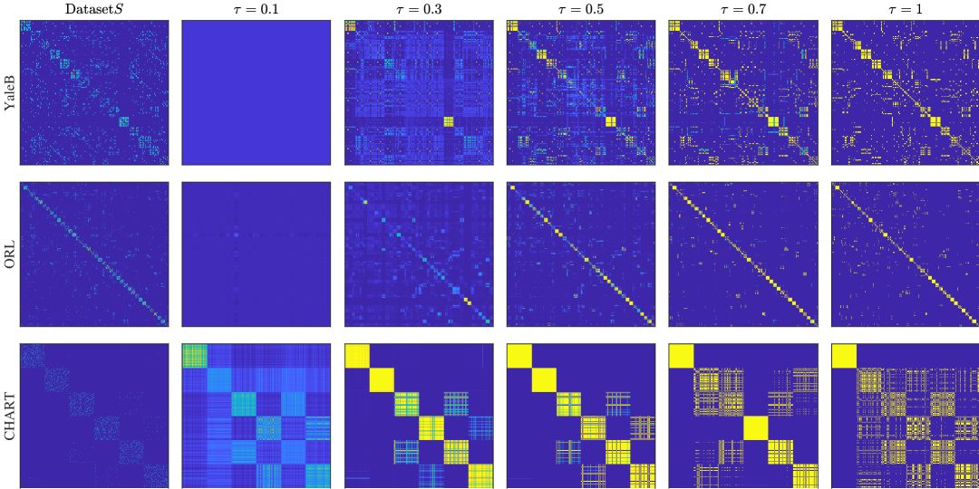
Figure 4: The visualization of learned $VV^{T}$ (normalized to $[0,1]$) with different $\tau$ of B-LoRD on the YaleB, ORL, and CHART datasets, zoom in for details.

How does $\tau$ control the block diagonality of $VV^{T}$? To investigate how $\tau$ (used in the computation of $\gamma$) controls the block diagonality of $VV^{T}$ learned by B-LoRD, we visualize $VV^{T}$ with different $\tau$ in Fig. 4, from which it can be observed that:

• The block diagonality of $VV^{T}$ increases with larger values of $\tau$, although the rate of increase varies across datasets. This variation may be attributed to specific properties of the similarity matrix $S$.

• When $\tau$ is sufficiently small (e.g., $\tau=0.1$), the learned $V\approx 1_{n}\mu^{T}/n$ and $VV^{T}\approx 1_{n}1_{n}^{T}/n^{2}$ exhibit no block diagonality. Theoretically, this trivial solution always arises when $\tau=0$.

• When $\tau$ is large, the learned $VV^{T}$ demonstrates strong block diagonality. For instance, with $\tau=0.7$ on the ORL dataset, the block structure becomes prominent. Notably, when $\tau=1$, the learned $VV^{T}$ is nearly block diagonal with each row of $V$ containing only a single non-zero element.

The influence of $\tau$ on clutering accuracy. The result is shown in Fig. 5, where $\tau_{0}=\frac{\lambda_{\max}(S)}{\lambda_{\max}(S)-\lambda_{\min}(S)}$. When $\tau>\tau_{0}$, $\gamma>0$ and the block diagonality is enhanced; when $\tau<\tau_{0}$, $\gamma<0$ and the block diagonality is weakened. Moreover, we visualized the learned $Z=n^{2}V\mathrm{Diag}(\mu\odot\mu)V^{T}$ of LoRD and B-LoRD on each dataset in Fig. 6, where the result of B-LoRD corresponds to the best $\tau$ achieving the highest ACC.

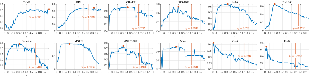
Figure 5: Values of ACC ($y$-axis) of B-LoRD with different values of $\tau$ ($x$-axis).

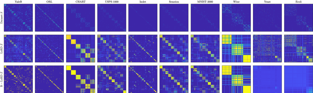
Figure 6: The visualization of learned $Z$ (normalized to $[0,1]$) of LoRD and B-LoRD on each datasets.

From Fig. 5 and Fig. 6, it can be seen that

• When the dataset is balanced, the optimal $\tau$ (corresponding to the highest ACC) is generally high, and the learned $Z$ exhibits high block-diagonality, especially on the YaleB, ORL, and CHART datasets.

• When the dataset is imbalanced, B-LoRD cannot find a suitable uniform partition, making small $\tau$ values perform well, especially on the Yeast and Ecoli datasets.

Practical adaptive selection strategy for $\tau$. As shown in Fig. 5, the value of ACC is sensitive to the choice of $\tau$, necessitating an adaptive hyperparameter selection strategy. Here we provide two practical guidelines for determining $\tau$:

• Based on sample size $n$: Empirical observations suggest that $\tau$ tends to decrease as the sample size $n$ increases. This leads to the first approximation strategy: $\hat{\tau}_{1}=\min\{2n^{-0.24},1\}$.

• Based on $n$ and the block-diagonality of $S$: Additionally, $\tau$ decreases with lower block-diagonality of $S$. We quantify block-diagonality using the metric $b=\sum_{i=1}^{k}\lambda_{i}(L_{S})/\mathrm{Tr}(L_{S})$, where $L_{S}=\mathrm{Diag}(S\mathbf{1}_{n})-S$ is the Laplacian of $S$. This metric can be efficiently computed when $S$ is sparse. By combining $b$ and $n$, we propose the second approximation: $\hat{\tau}_{2}=\min\{0.34\exp(50b-0.03\log n),1\}$.

The values of $\hat{\tau}_{1}$, $\hat{\tau}_{2}$, and the optimal $\tau^{\ast}$ for each dataset are presented in Table 4, where MAE stands for Mean Absolute Error. The corresponding clustering ACC values of B-LoRD for $\hat{\tau}_{1}$, $\hat{\tau}_{2}$, and $\tau^{\ast}$ are reported in Table 5. From Table 4 and Table 5, it can be observed that when using $\hat{\tau}_{1}$ and $\hat{\tau}_{2}$, the MAE values were $0.16$ and $0.13$, respectively, while the average ACC decreases by only $0.05$ and $0.045$ accordingly. These results validate the effectiveness of the proposed adaptive strategies.

Table 4: The values of $\hat{\tau}_{1}$, $\hat{\tau}_{2}$ and $\tau^{\ast}$.

	D1	D2	D3	D4	D5	D6	D7	D8	D9	D10	D11	D12	MAE
$\hat{\tau}_{1}$	$0.59$	$0.47$	$0.43$	$0.38$	$0.23$	$0.24$	$0.34$	$0.14$	$0.32$	$0.58$	$0.35$	$0.50$	$0.16$
$\hat{\tau}_{2}$	$0.83$	$0.95$	$0.28$	$0.29$	$0.26$	$0.26$	$0.28$	$0.24$	$0.27$	$0.30$	$0.28$	$0.30$	$0.13$
$\tau^{\ast}$	$0.83$	$0.62$	$0.44$	$0.28$	$0.34$	$0.22$	$0.42$	$0.34$	$0.38$	$0.43$	$0.04$	$0.03$	$0$

Table 5: The clustering ACC values of B-LoRD corresponding to $\hat{\tau}_{1}$, $\hat{\tau}_{2}$ and $\tau^{\ast}$.

ACC	D1	D2	D3	D4	D5	D6	D7	D8	D9	D10	D11	D12	Avg.
$\hat{\tau}_{1}$	$0.509$	$0.637$	$0.905$	$0.633$	$0.627$	$0.629$	$0.782$	$0.954$	$0.716$	$0.848$	$0.304$	$0.500$	$0.670$
$\hat{\tau}_{2}$	$0.485$	$0.628$	$0.890$	$0.719$	$0.633$	$0.608$	$0.693$	$0.962$	$0.702$	$0.949$	$0.321$	$0.509$	$0.675$
$\tau^{\ast}$	$0.515$	$0.685$	$0.905$	$0.740$	$0.644$	$0.647$	$0.783$	$0.964$	$0.745$	$0.955$	$0.412$	$0.741$	$0.720$

5.5 Robustness to Data Imbalance

In our experiments, we used $\mu_{0}=[1/\sqrt{k},\dots,1/\sqrt{k}]^{T}$ because $\mu^{\ast}=[\sqrt{\pi_{1}},\dots,\sqrt{\pi_{k}}]^{T}$ was unknown. This setting may lead to misleading clustering results when the dataset is significantly imbalanced. To analyze the performance gap of LoRD and B-LoRD between $\mu_{0}$ and $\mu^{\ast}$ on imbalanced datasets, we define the imbalance rate (IBR) as:

$$\mathrm{IBR}=1-\mathcal{H}(\bm{\pi})/\log k,$$ (32)

where $\mathcal{H}(\bm{\pi})=-\sum_{i=1}^{k}\bm{\pi}_{i}\log\bm{\pi}_{i}$ is the entropy of $\bm{\pi}$, and the normalization factor $\log k$ ensures that $\mathrm{IBR}\in[0,1]$.

As shown in Table 6, the performance gap generally increases as IBR increases. Meanwhile, B-LoRD is more robust to IBR than LoRD, because the block diagonality of $VV^{T}$ can be adapted by tuning $\tau\in[0,1]$ to alleviate this effect. Please see the detailed discussion in Appendix 5.4.

Table 6: The gap of ACC on imbalanced datasets.

Datasets	Semeion	MNIST-2000	Wine	Yeast	Ecoli
IBR	$3\times 10^{-5}$	$0.0014$	$0.0114$	$0.2503$	$0.2704$
LoRD-$\mu_{0}$	$0.755$	$0.657$	$0.944$	$0.303$	$0.455$
LoRD-$\mu^{\ast}$	$0.755$	$0.669$	$0.916$	$0.385$	$0.717$
LoRD-gap	$0$	$0.008$	$\!\!-0.028\;\,$	$0.082$	$0.262$
B-LoRD-$\mu_{0}$	$0.783$	$0.745$	$0.955$	$0.412$	$0.741$
B-LoRD-$\mu^{\ast}$	$0.783$	$0.742$	$0.933$	$0.470$	$0.801$
B-LoRD-gap	$0$	$\!\!-0.003\;\,$	$\!\!-0.022\;\,$	$0.058$	$0.060$

5.6 Convergence Analysis

The convergence behaviors of the proposed Alg. 1 are shown in Fig. 7 and Fig. 8, with Fig. 8 representing the results obtained using the optimal hyperparameter. From these results, we observe that the objective function value decreases monotonically in Fig. 7 and increases monotonically in Fig. 8, typically reaching convergence within a few hundred iterations.

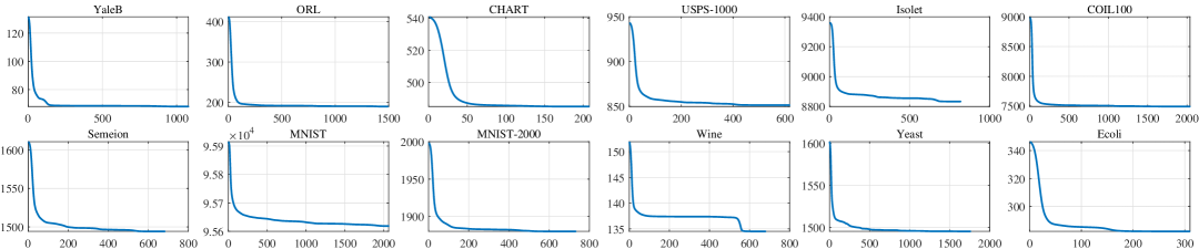
Figure 7: Convergence curves of LoRD on ten datasets. For each dataset, the $x$-axis represents the iteration count, and the $y$-axis represents the objective function of Eq. (17).

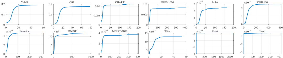
Figure 8: Convergence curves of B-LoRD on ten datasets. For each dataset, the $x$-axis represents the iteration count, and the $y$-axis represents the objective function of Eq. (20).

5.7 Synthetic Experiment

We generated $200$ samples from four Gaussian distributions: $\mathcal{N}\left(\begin{bmatrix}-2\\ 2\end{bmatrix},\begin{bmatrix}0.25&0\\ 0&0.25\end{bmatrix}\right)$, $\mathcal{N}\left(\begin{bmatrix}2\\ 2\end{bmatrix},\begin{bmatrix}1&0\\ 0&1\end{bmatrix}\right)$, $\mathcal{N}\left(\begin{bmatrix}-2\\ -2\end{bmatrix},\begin{bmatrix}1&0\\ 0&1\end{bmatrix}\right)$ and $\mathcal{N}\left(\begin{bmatrix}2\\ -2\end{bmatrix},\begin{bmatrix}2.25&0\\ 0&2.25\end{bmatrix}\right)$. We set five different values of $\bm{\pi}$ to obtain different IBRs, as shown in Table 7.

Table 7: Clustering ACC of synthetic experiment.

$n\bm{\pi}$	IBR	GMM		LoRD		B-LoRD
		$\mu^{\ast}$	$\mu_{0}$	$\mu^{\ast}$	$\mu_{0}$	$\mu^{\ast}$	$\mu_{0}$
$[50,50,50,50]$	$0$	$0.935$	$0.935$	$0.940$	$0.940$	$0.960$	$0.960$
$[40,50,50,60]$	$0.0073$	$0.960$	$0.945$	$0.945$	$0.920$	$0.945$	$0.935$
$[30,45,55,70]$	$0.0315$	$0.925$	$0.895$	$0.860$	$0.800$	$0.865$	$0.880$
$[20,40,60,80]$	$0.0768$	$0.780$	$0.835$	$0.870$	$0.740$	$0.890$	$0.790$
$[10,30,60,100]$	$0.1761$	$0.840$	$0.745$	$0.885$	$0.620$	$0.900$	$0.700$

The clustering results for the case of $n\bm{\pi}=[20,40,60,80]$ are plotted in Fig. 9, where the similarity matrix $S=X^{T}X$.

Figure 9: The sampled data and the clustering result of LoRD for the case of $n\bm{\pi}=[20,40,60,80]$. The color and opacity of a data point represent its cluster and clustering probability, respectively.

From Table 7 and Fig. 9, it can be observed that:

• Regardless of whether $\mu^{\ast}$ or $\mu_{0}$ are provided in LoRD, samples close to the cluster center have high clustering probabilities, while those at the intersection of multiple clusters show low clustering probabilities.

• When $\mu_{0}$ deviates from $\mu^{\ast}$, LoRD fails to find a suitable uniform partition, resulting in a low clustering probability for a large number of samples.

• As the IBR increases, the performance gap between LoRD and B-LoRD with given $\mu^{\ast}$ and $\mu_{0}$ becomes more pronounced.

Please see the detailed results and analyses in Appendix A.1.

6 Conclusion and Discussion

In this paper, we introduced LoRD, a novel graph-based clustering model, by relaxing the least crucial orthonormal constraint of kernel $k$-means, which is further enhanced by integrating adjustable block diagonality, leading to B-LoRD. To tackle numerical challenges, we theoretically elucidated how the non-convex doubly stochastic constraint can be reduced to a convex constraint by introducing the class probability parameter $\mu$. Additionally, leveraging the gradient Lipschitz continuity property, we devised a projected gradient descent algorithm for the effective resolution of LoRD and B-LoRD, which theoretically ensures global convergence.

Despite the effectiveness of LoRD and B-LoRD, a practical hurdle remains as $\mu^{\ast}$ is typically unknown in real-world applications. Moving forward, our research will delve into methods for accurately estimating $\mu^{\ast}$ to reduce the impact of estimated biases on model performance.

Appendix A Additional Experimental Results

A.1 Additional Synthetic Experiment

In Tables 8, 9 and 10, we list the clustering performances of GMM, LoRD and B-LoRD in the synthetic experiment, respectively. Moreover, the clustering results of LoRD are shown in Fig. 10.

Table 8: Clustering performance of GMM in synthetic experiment.

$n\bm{\pi}$	IBR	ACC			NMI			PUR			F1
		$\mu^{\ast}$	$\mu_{0}$	gap	$\mu^{\ast}$	$\mu_{0}$	gap	$\mu^{\ast}$	$\mu_{0}$	gap	$\mu^{\ast}$	$\mu_{0}$	gap
$[50,50,50,50]$	0	0.935	0.935	0	0.832	0.832	0	0.935	0.935	0	0.879	0.879	0
$[40,50,50,60]$	0.0073	0.960	0.945	0.015	0.877	0.847	0.030	0.960	0.945	0.015	0.916	0.887	0.029
$[30,45,55,70]$	0.0315	0.925	0.895	0.030	0.783	0.739	0.044	0.925	0.895	0.030	0.847	0.791	0.056
$[20,40,60,80]$	0.0768	0.780	0.835	-0.055	0.672	0.708	-0.036	0.820	0.835	-0.015	0.747	0.739	0.078
$[10,30,60,100]$	0.1761	0.840	0.745	0.095	0.657	0.506	0.151	0.840	0.745	0.095	0.713	0.623	0.090

Table 9: Clustering performance of LoRD in synthetic experiment.

$n\bm{\pi}$	IBR	ACC			NMI			PUR			F1
		$\mu^{\ast}$	$\mu_{0}$	gap	$\mu^{\ast}$	$\mu_{0}$	gap	$\mu^{\ast}$	$\mu_{0}$	gap	$\mu^{\ast}$	$\mu_{0}$	gap
$[50,50,50,50]$	0	0.940	0.940	0	0.838	0.838	0	0.940	0.940	0	0.887	0.887	0
$[40,50,50,60]$	0.0073	0.945	0.920	0.025	0.844	0.786	0.058	0.945	0.920	0.025	0.887	0.845	0.042
$[30,45,55,70]$	0.0315	0.860	0.800	0.060	0.721	0.590	0.131	0.860	0.800	0.060	0.735	0.659	0.076
$[20,40,60,80]$	0.0768	0.870	0.740	0.130	0.724	0.552	0.172	0.870	0.740	0.130	0.749	0.597	0.152
$[10,30,60,100]$	0.1761	0.885	0.620	0.265	0.651	0.496	0.155	0.885	0.775	0.110	0.802	0.552	0.250

Table 10: Clustering performance of B-LoRD in synthetic experiment.

$n\bm{\pi}$	IBR	ACC			NMI			PUR			F1
		$\mu^{\ast}$	$\mu_{0}$	gap	$\mu^{\ast}$	$\mu_{0}$	gap	$\mu^{\ast}$	$\mu_{0}$	gap	$\mu^{\ast}$	$\mu_{0}$	gap
$[50,50,50,50]$	0	0.960	0.960	0	0.884	0.884	0	0.960	0.960	0	0.923	0.923	0
$[40,50,50,60]$	0.0073	0.945	0.935	0.010	0.861	0.840	0.021	0.945	0.935	0.010	0.888	0.871	0.017
$[30,45,55,70]$	0.0315	0.865	0.880	-0.015	0.740	0.711	0.029	0.865	0.880	-0.015	0.743	0.770	-0.027
$[20,40,60,80]$	0.0768	0.890	0.790	0.100	0.752	0.631	0.121	0.890	0.820	0.070	0.787	0.682	0.105
$[10,30,60,100]$	0.1761	0.900	0.700	0.200	0.681	0.535	0.146	0.900	0.805	0.095	0.823	0.634	0.189

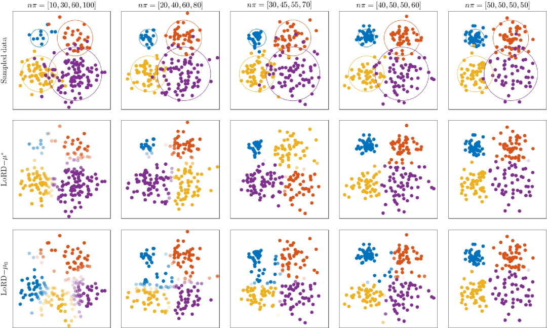
Figure 10: Clustering result of LoRD in synthetic experiment. The four clusters are marked with different colors, and the opacity is set to the cluster probability $\mathrm{P}(y_{j}|x_{i})$.

Additionally, from Tables 8, 9 and 10, it can be seen that B-LoRD is more robust to the deviation between $\mu_{0}$ and $\mu^{\ast}$. To study its mechanism, we provide the hyper-parameter analysis of B-LoRD in the synthetic experiment, as shown in Fig. 11, and the clustering result under the optimal hyper-parameter is shown in Fig. 12. From these results, we observe that:

• When $\mu^{\ast}$ is known, B-LoRD achieves high ACC when $\tau$ is large, i.e., the learned $VV^{T}$ exhibits high $k$-block diagonality.

• When $\mu_{0}$ deviates from $\mu^{\ast}$, B-LoRD cannot find a suitable uniform partition, resulting in better performance for a smaller $\tau$. This is because, when the $k$-block diagonality of $VV^{T}$ is weakened, the learned partition ratios do not strictly obey $\mu_{0}$. For example, as shown in the third row of Fig. 12, in the cases of $n\pi=[20,40,60,80]$ and $n\pi=[30,45,55,70]$, the partition corresponding to the blue-colored cluster is almost correct. Moreover, for $n\pi=[10,30,60,100]$, the blue-colored cluster vanishes. Therefore, by tuning $\tau$, B-LoRD can enhance or weaken the block diagonality, and thereby reduce the impact of the deviation between $\mu_{0}$ and $\mu^{\ast}$.

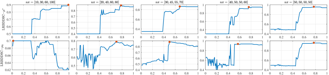
Figure 11: Values of ACC ($y$-axis) of B-LoRD with different values of $\tau$ ($x$-axis) in synthetic experiments. The optimal $\tau$ corresponding to highest ACC is marked with an orange point.

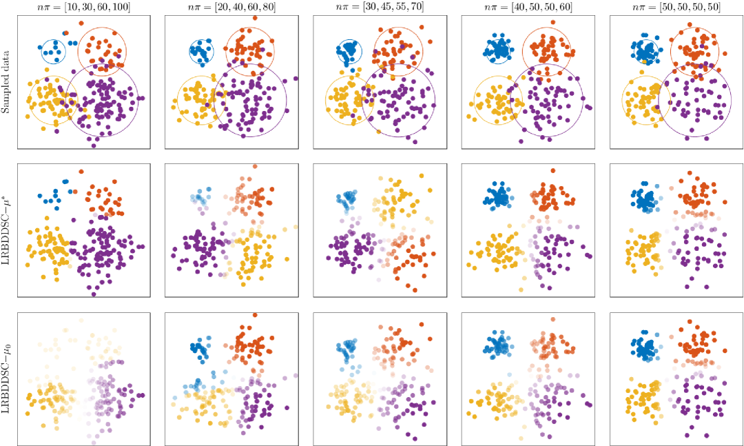
Figure 12: Clustering results of B-LoRD in synthetic datasets. The four clusters are marked with different colors, and the opacity is set to the cluster probability $\mathrm{P}(y_{j}|x_{i})$.

A.2 Clustering Results

The clustering NMI, PUR and F1 scores of all methods on each dataset are shown in Table 11, Table 12 and Table 13, respectively. The analyses of these results are consistent with the discussions in Sec. 5.2.

Table 11: NMI on each dataset.

NMI	D1	D2	D3	D4	D5	D6	D7	D8	D9	D10	D11	D12	Avg.
KKM	$0.534$	$0.765$	$0.794$	$0.525$	$0.741$	$0.762$	$0.578$	$0.582$	$0.561$	$0.799$	$0.239$	$0.592$	$0.599$
GKKM	$0.415$	$0.692$	$0.788$	$0.543$	$0.763$	$0.622$	$0.534$	$-$	$0.565$	$0.822$	$0.239$	$0.618$	$0.580$
SDP	$0.555$	$0.807$	$0.819$	$0.576$	$-$	$-$	$0.590$	$-$	$0.612$	$0.763$	$0.260$	$0.550$	$-$
DCD	$0.526$	$0.798$	$0.806$	$0.602$	$0.758$	$0.822$	$0.620$	$0.744$	$0.671$	$0.851$	$0.256$	$0.627$	$0.640$
SC	$0.537$	$0.798$	$0.795$	$0.587$	$0.764$	$0.823$	$0.660$	$0.755$	$0.670$	$0.825$	$0.265$	$0.588$	$0.636$
SR	$0.534$	$0.794$	$0.795$	$0.579$	$0.765$	$0.814$	$0.607$	$0.743$	$0.665$	$0.825$	$0.278$	$0.632$	$0.634$
NCut	$0.532$	$0.798$	$0.795$	$0.569$	$0.766$	$0.793$	$0.607$	$0.751$	$0.663$	$0.813$	$0.283$	$0.617$	$0.631$
DBSC	$0.547$	$0.801$	$0.814$	$0.558$	$0.758$	$0.792$	$0.647$	$-$	$0.590$	$0.828$	$0.282$	$0.581$	$0.628$
DirectSC	$0.518$	$0.792$	$0.809$	$0.522$	$0.637$	$-$	$0.495$	$-$	$0.423$	$0.718$	$0.257$	$0.620$	$0.573$
SymNMF	$0.532$	$0.806$	$0.814$	$0.539$	$0.726$	$0.774$	$0.614$	$0.532$	$0.573$	$0.781$	$0.266$	$0.574$	$0.611$
PHALS	$0.534$	$0.803$	$0.767$	$0.528$	$0.755$	$0.798$	$0.647$	$0.689$	$0.609$	$0.798$	$0.279$	$0.575$	$0.616$
S3NMF	$0.525$	$0.791$	$0.816$	$0.562$	$-$	$-$	$0.665$	$-$	$0.636$	$0.819$	$0.260$	$0.592$	$0.630$
NLR	$0.536$	$0.800$	$0.591$	$0.517$	$0.541$	$-$	$0.550$	$-$	$0.485$	$0.802$	$0.240$	$0.800$	$0.591$
DSN	$0.540$	$0.799$	$0.795$	$0.589$	$0.765$	$0.822$	$0.660$	$-$	$0.669$	$0.825$	$0.264$	$0.589$	$0.637$
SDS	$0.580$	$0.835$	$0.845$	$0.651$	$-$	$-$	$0.671$	$-$	$0.665$	$0.865$	$0.270$	$0.637$	$0.669$
DvD	$0.499$	$0.783$	$0.696$	$0.478$	$-$	$-$	$0.570$	$-$	$0.527$	$0.877$	$0.232$	$0.573$	$0.582$
DSNI	$0.540$	$0.806$	$0.805$	$0.647$	$-$	$-$	$0.655$	$-$	$0.697$	$0.696$	$0.263$	$0.610$	$0.635$
DSDC	$0.487$	$0.759$	$0.796$	$0.453$	$0.733$	$0.779$	$0.560$	$0.500$	$0.522$	$0.713$	$0.247$	$0.585$	$0.569$
LoRD (ours)	$0.518$	$0.798$	$0.827$	$0.579$	$0.758$	$0.774$	$0.681$	$0.883$	$0.614$	$0.807$	$0.256$	$0.530$	$0.623$
B-LoRD (ours)	$0.564$	$0.824$	$0.850$	$0.678$	$0.794$	$0.831$	$0.696$	$0.910$	$0.683$	$0.853$	$0.279$	$0.621$	$0.672$

Table 12: PUR on each dataset.

PUR	D1	D2	D3	D4	D5	D6	D7	D8	D9	D10	D11	D12	Avg.
KKM	$0.491$	$0.628$	$0.835$	$0.547$	$0.607$	$0.530$	$0.618$	$0.657$	$0.651$	$0.944$	$0.513$	$0.801$	$0.670$
GKKM	$0.364$	$0.568$	$0.667$	$0.560$	$0.643$	$0.339$	$0.553$	$-$	$0.646$	$0.944$	$0.497$	$0.813$	$0.624$
SDP	$0.516$	$0.687$	$0.762$	$0.604$	$-$	$-$	$0.646$	$-$	$0.677$	$0.916$	$0.526$	$0.797$	$-$
DCD	$0.461$	$0.670$	$0.667$	$0.623$	$0.604$	$0.641$	$0.648$	$0.736$	$0.728$	$0.955$	$0.521$	$0.836$	$0.679$
SC	$0.467$	$0.669$	$0.667$	$0.615$	$0.608$	$0.648$	$0.714$	$0.750$	$0.732$	$0.949$	$0.519$	$0.826$	$0.684$
SR	$0.467$	$0.670$	$0.667$	$0.609$	$0.601$	$0.636$	$0.635$	$0.737$	$0.727$	$0.949$	$0.514$	$0.839$	$0.675$
NCut	$0.467$	$0.683$	$0.667$	$0.593$	$0.602$	$0.596$	$0.638$	$0.741$	$0.726$	$0.949$	$0.517$	$0.836$	$0.675$
DBSC	$0.473$	$0.685$	$0.842$	$0.594$	$0.612$	$0.599$	$0.689$	$-$	$0.663$	$0.944$	$0.549$	$0.824$	$0.696$
DirectSC	$0.452$	$0.647$	$0.667$	$0.497$	$0.489$	$-$	$0.505$	$-$	$0.480$	$0.899$	$0.520$	$0.827$	$0.610$
SymNMF	$0.479$	$0.690$	$0.842$	$0.588$	$0.587$	$0.556$	$0.670$	$0.586$	$0.674$	$0.916$	$0.530$	$0.824$	$0.690$
PHALS	$0.479$	$0.683$	$0.800$	$0.567$	$0.616$	$0.588$	$0.690$	$0.676$	$0.690$	$0.927$	$0.553$	$0.819$	$0.690$
S3NMF	$0.485$	$0.664$	$0.817$	$0.629$	$-$	$-$	$0.712$	$-$	$0.678$	$0.935$	$0.539$	$0.827$	$0.698$
NLR	$0.503$	$0.687$	$0.645$	$0.502$	$0.430$	$-$	$0.560$	$-$	$0.489$	$0.938$	$0.458$	$0.687$	$0.608$
DSN	$0.470$	$0.669$	$0.667$	$0.619$	$0.609$	$0.647$	$0.713$	$-$	$0.732$	$0.949$	$0.520$	$0.826$	$0.685$
SDS	$0.515$	$0.710$	$0.847$	$0.638$	$-$	$-$	$0.740$	$-$	$0.719$	$0.961$	$0.545$	$0.843$	$0.724$
DvD	$0.455$	$0.668$	$0.680$	$0.510$	$-$	$-$	$0.602$	$-$	$0.522$	$0.966$	$0.449$	$0.816$	$0.630$
DSNI	$0.472$	$0.669$	$0.667$	$0.649$	$-$	$-$	$0.708$	$-$	$0.747$	$0.899$	$0.528$	$0.817$	$0.684$
DSDC	$0.418$	$0.600$	$0.695$	$0.489$	$0.609$	$0.559$	$0.644$	$0.601$	$0.626$	$0.888$	$0.521$	$0.817$	$0.633$
LoRD (ours)	$0.479$	$0.683$	$0.878$	$0.613$	$0.610$	$0.538$	$0.755$	$0.943$	$0.657$	$0.944$	$0.522$	$0.783$	$0.702$
B-LoRD (ours)	$0.521$	$0.703$	$0.905$	$0.748$	$0.658$	$0.659$	$0.783$	$0.964$	$0.747$	$0.955$	$0.561$	$0.833$	$0.751$

Table 13: F1-score on each dataset.

F1	D1	D2	D3	D4	D5	D6	D7	D8	D9	D10	D11	D12	Avg.
KKM	$0.325$	$0.453$	$0.752$	$0.413$	$0.518$	$0.404$	$0.471$	$0.540$	$0.486$	$0.888$	$0.243$	$0.502$	$0.504$
GKKM	$0.165$	$0.216$	$0.688$	$0.409$	$0.566$	$0.109$	$0.436$	$-$	$0.478$	$0.889$	$0.249$	$0.557$	$0.454$
SDP	$0.339$	$0.538$	$0.718$	$0.450$	$-$	$-$	$0.478$	$-$	$0.513$	$0.838$	$0.267$	$0.445$	$-$
DCD	$0.308$	$0.521$	$0.695$	$0.496$	$0.524$	$0.489$	$0.497$	$0.668$	$0.600$	$0.909$	$0.250$	$0.524$	$0.533$
SC	$0.317$	$0.520$	$0.691$	$0.481$	$0.520$	$0.528$	$0.567$	$0.667$	$0.600$	$0.898$	$0.264$	$0.476$	$0.535$
SR	$0.317$	$0.512$	$0.691$	$0.470$	$0.500$	$0.446$	$0.482$	$0.653$	$0.592$	$0.898$	$0.296$	$0.541$	$0.533$
NCut	$0.313$	$0.531$	$0.691$	$0.455$	$0.500$	$0.313$	$0.483$	$0.658$	$0.591$	$0.887$	$0.291$	$0.523$	$0.529$
DBSC	$0.328$	$0.538$	$0.765$	$0.447$	$0.525$	$0.475$	$0.562$	$-$	$0.528$	$0.887$	$0.281$	$0.467$	$0.534$
DirectSC	$0.293$	$0.460$	$0.699$	$0.380$	$0.369$	$-$	$0.388$	$-$	$0.343$	$0.811$	$0.286$	$0.548$	$0.468$
SymNMF	$0.313$	$0.540$	$0.765$	$0.436$	$0.493$	$0.418$	$0.536$	$0.454$	$0.525$	$0.838$	$0.268$	$0.465$	$0.521$
PHALS	$0.313$	$0.534$	$0.708$	$0.411$	$0.523$	$0.461$	$0.570$	$0.605$	$0.549$	$0.857$	$0.281$	$0.461$	$0.520$
S3NMF	$0.320$	$0.511$	$0.757$	$0.482$	$-$	$-$	$0.605$	$-$	$0.583$	$0.880$	$0.268$	$0.509$	$0.546$
NLR	$0.315$	$0.470$	$0.514$	$0.313$	$0.152$	$-$	$0.320$	$-$	$0.264$	$0.877$	$0.322$	$0.470$	$0.429$
DSN	$0.321$	$0.521$	$0.691$	$0.484$	$0.517$	$-$	$0.566$	$-$	$0.599$	$0.898$	$0.262$	$0.477$	$0.535$
SDS	$0.368$	$0.551$	$0.771$	$0.521$	$-$	$-$	$0.601$	$-$	$0.587$	$0.923$	$0.398$	$0.673$	$0.599$
DvD	$0.251$	$0.302$	$0.587$	$0.342$	$-$	$-$	$0.323$	$-$	$0.338$	$0.931$	$0.318$	$0.533$	$0.436$
DSNI	$0.321$	$0.514$	$0.694$	$0.523$	$-$	$-$	$0.567$	$-$	$0.622$	$0.809$	$0.255$	$0.541$	$0.538$
DSDC	$0.264$	$0.414$	$0.697$	$0.364$	$0.516$	$0.474$	$0.484$	$0.451$	$0.465$	$0.793$	$0.243$	$0.491$	$0.468$
LoRD (ours)	$0.308$	$0.535$	$0.802$	$0.491$	$0.560$	$0.436$	$0.638$	$0.893$	$0.548$	$0.888$	$0.243$	$0.430$	$0.543$
B-LoRD (ours)	$0.355$	$0.593$	$0.837$	$0.633$	$0.608$	$0.576$	$0.656$	$0.930$	$0.640$	$0.913$	$0.365$	$0.744$	$0.637$

A.3 Complexity of Dykstra Algorithm 2

As analyzed in Sec. 4.6, the complexity of the Dykstra Algorithm 2 is $\mathcal{O}(nkb_{\text{avg}})$, where $b_{\text{avg}}$ is the average iteration count. In this subsection, we summarize $b_{\text{avg}}$ for LoRD and B-LoRD on each dataset, as shown in Fig. 13. From Fig. 13, we observed that: The $b_{\text{avg}}$ of LoRD is approximately $50$, independent of $n$ but proportional to $k$. The $b_{\text{avg}}$ of B-LoRD varies more significantly, ranging from approximately $50$ to $500$, and appears to be independent of both $n$ and $k$.

(a)

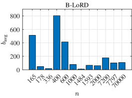
(b)

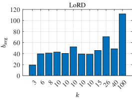
(c)

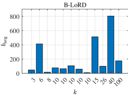
(d)

Figure 13: The correlation between $b_{\text{avg}}$ ($y$-axis) and number of samples $n$ and classes $k$ ($x$-axis, sorted in ascending order).

A.4 Correlation between Objective Function Value and ACC

The relationship between the objective function value and the clustering ACC of SR, SymNMF, PHALS, LoRD and B-LoRD are described in Fig. 14 to Fig. 19, respectively. In general, the correlation (measured by $\mathrm{R}^{2}$) in KKM, LoRD and B-LoRD is stronger than SR, SymNMF and PHALS, because the doubly stochastic constraint is relaxed in SR, SymNMF and PHALS.

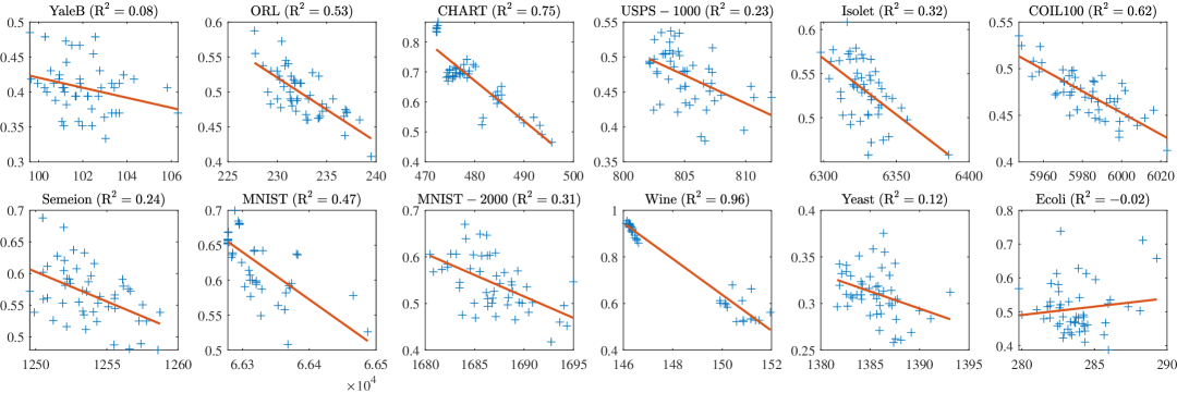
Figure 14: Correlation of objective function and clustering ACC in KKM.

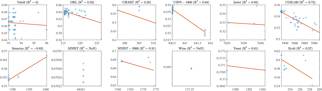
Figure 15: Correlation of objective function and clustering ACC in SR.

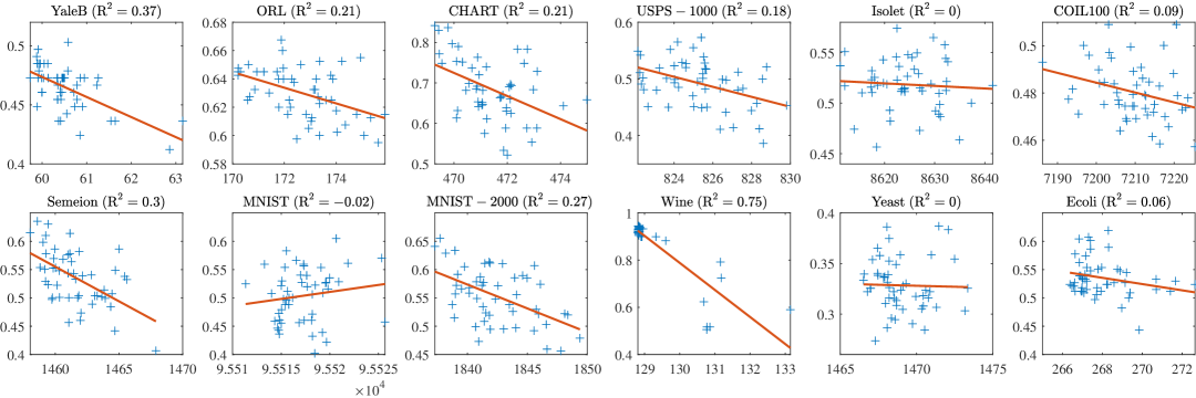
Figure 16: Correlation of objective function and clustering ACC in SymNMF.

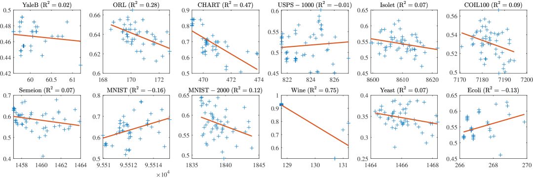
Figure 17: Correlation of objective function and clustering ACC in PHALS.

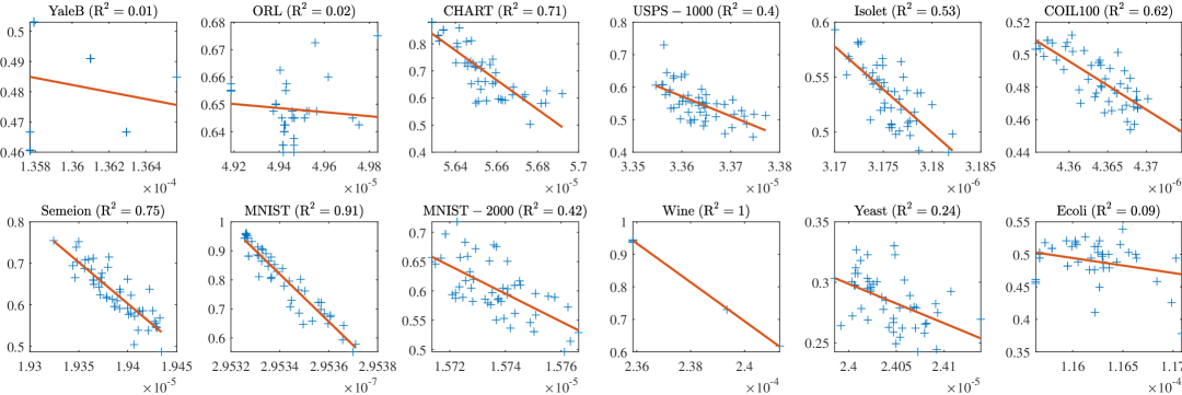
Figure 18: Correlation of objective function and clustering ACC in LoRD.

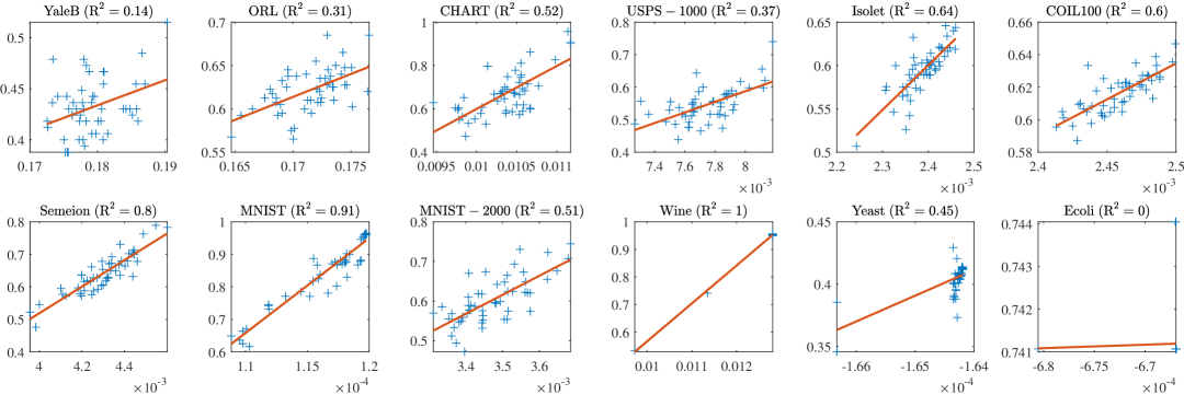
Figure 19: Correlation of objective function and clustering ACC in B-LoRD.

Appendix B Proofs

B.1 Proof of Theorem 1

Proof The proof is straightforward; the three conditions in Theorem 1 are proven as follows:

• First, for all $\mu\in\mathbb{S}_{+}^{k}$, we can construct $1_{n}\mu^{T}/n\in\Omega(\mu)$, which shows that $\Omega(\mu)\neq\emptyset$.

• Second, $\Omega(\mu)$ is a subspace of $\Omega$, which shows that $\bigcup_{\mu\in\mathbb{S}_{+}^{k}}\Omega(\mu)\subseteq\Omega$. Moreover, for all $V\in\Omega$, we have $1_{n}^{T}VV^{T}1_{n}=1\Rightarrow V^{T}1_{n}\in\mathbb{S}_{+}^{k}$, thus $V\in\Omega(V^{T}1_{n})$, which implies that $\Omega\subseteq\bigcup_{\mu\in\mathbb{S}_{+}^{k}}\Omega(\mu)$. Thus, $\Omega=\bigcup_{\mu\in\mathbb{S}_{+}^{k}}\Omega(\mu)$ holds.

• Third, suppose $V\in\Omega(\mu)$ and $V\in\Omega(\nu)$, we have $V^{T}1_{n}=\mu=\nu$, which contradicts the condition $\mu\neq\nu$. Therefore, $\Omega(\mu)\cap\Omega(\nu)=\emptyset$.

 

B.2 Proof of Theorem 2

Proof Let $\mu=[\sqrt{\mathrm{P}(c_{1})},\dots,\sqrt{\mathrm{P}(c_{j})}]^{T}$, $\mathrm{P}(x_{i})=1_{n}/n$ and $V_{ij}=\frac{\mathrm{P}(y_{i}=j|x_{i})\mathrm{P}(x_{i})}{\sqrt{\mathrm{P}(c_{j})}}$. According to $\mathrm{P}(y_{i}=j|x_{i})\mathrm{P}(x_{i})=\mathrm{P}(x_{i}|y_{i}=j)\mathrm{P}(c_{j})$, we have:

$$(V\mu)_{i} =\mathrm{P}(x_{i})\sum_{j=1}^{k}\mathrm{P}(y_{i}=j|x_{i})=\mathrm{P}(x_{i})=\frac{1}{n}.$$ (33)

$$(V^{T}1_{n})_{j} =\sum_{i=1}^{n}\frac{\mathrm{P}(y_{i}=j|x_{i})\mathrm{P}(x_{i})}{\sqrt{\mathrm{P}(c_{j})}}=\sqrt{\mathrm{P}(c_{j})}\sum_{i=1}^{n}\mathrm{P}(x_{i}|y_{i}=j)=\sqrt{\mathrm{P}(c_{j})}=\mu_{j},$$

which indicate that $V\in\Omega(\mu)$.

Moreover, let $Z=n^{2}V\mathrm{Diag}(\mu\odot\mu)V^{T}$. Under the conditional independence assumption, i.e., $\mathrm{P}(y_{i}|x_{i})=\mathrm{P}(y_{i}|x_{i},x_{j})$ and $\mathrm{P}(y_{i},y_{j}|x_{i},x_{j})=\mathrm{P}(y_{i}|x_{i},x_{j})\mathrm{P}(y_{j}|x_{i},x_{j})$, we have

$$Z_{ij}=\sum_{a=1}^{k}\mathrm{P}(y_{i}=a|x_{i})\mathrm{P}(y_{j}=a|x_{j})=\sum_{a=1}^{k}\mathrm{P}(y_{i}=a,y_{j}=a|x_{i},x_{j})=\mathrm{P}(y_{i}=y_{j}|x_{i},x_{j}).$$ (34)

 

B.3 Proof of Theorem 4

Proof Given $V\in\Omega$, we have the Laplacian of $VV^{T}$ is:

$$L_{VV^{T}}:=\mathrm{Diag}(VV^{T}1_{n})-VV^{T}=1_{n}/n-VV^{T}.$$ (35)

Therfore, the first $n-k$ largest eigenvalues of $L_{VV^{T}}$ are all $1/n$, and the last $k$ eiganvalues are:

$$\lambda_{n-i+1}(L_{VV^{T}})=\frac{1}{n}-\lambda_{i}(VV^{T})=\frac{1}{n}-\sigma_{i}^{2}(V),\quad i=1,\dots,k.$$ (36)

Accordingly, $\|VV^{T}\|_{\hbox to6.82pt{\vbox to7.26pt{\text{[drawing]}}}}$ can be simplified as:

$$\sum_{i=1}^{k}\lambda_{n\!-\!i\!+\!1}(L_{VV^{T}})=\frac{k}{n}\!-\!\sum_{i=1}^{k}\sigma_{i}^{2}(V)\!=\!\frac{k}{n}-\|V\|_{F}^{2}.$$ (37)

Moreover, according to $\mathcal{P}_{\Omega_{0}(\mu)}(U)$ given in Lemma 7, the least $k$-block diagonal case is $1_{n}\mu^{T}/n=\mathcal{P}_{\Omega_{0}(\mu)}(0_{n\times k})=\arg\min_{V\in\Omega(\mu)}\|V\|_{F}^{2}$, where $0_{n\times k}$ is an $n\times k$ matrix with all zeros. For all $\mu\in\mathbb{S}_{+}^{k}$, the $k$-block diagonality of $1_{n}\mu^{T}/n$ are equal, i.e., $\|1_{n}\mu^{T}/n\|_{F}^{2}=1/n$.

The fully $k$-block diagonal case occurs when $V$ is orthogonal. For example, given a partition $G_{1},\dots,G_{k}$, let $V_{ij}=1/\sqrt{n\times n_{j}}$ if $x_{i}\in G_{j}$ and zero otherwise. Then, $\|V\|_{F}^{2}=\frac{k}{n}$, which implies that $\|VV^{T}\|_{\hbox to6.82pt{\vbox to7.26pt{\text{[drawing]}}}}=0$.  

B.4 Proof of Theorem 6

Proof To show that $\nabla_{1}=4(VV^{T}-S)V$ and $\nabla_{2}=-2(SV+\gamma V)$ are $L_{1}$- and $L_{2}$-Lipschitz continuous on $\Omega$, respectively, we need to prove:

$$\forall V,U\in\Omega(\mu),\quad\begin{cases}\|\nabla_{1}(V)-\nabla_{1}(U)\|_{F}\leq 4\left(3/n+\|S\|_{\mathrm{op}}\right)\|V-U\|_{F}\\ \|\nabla_{2}(V)-\nabla_{2}(U)\|_{F}\leq 2\left\|S+\gamma I_{n}\right\|_{\mathrm{op}}\|V-U\|_{F}\end{cases},$$ (38)

where $\|\cdot\|_{\mathrm{op}}$ denotes the operator norm, i.e., the largest singular value of matrix. For $\nabla_{2}$, the proof is straightforward:

$$\|\nabla_{2}(V)-\nabla_{2}(U)\|_{F}=\|2(S+\gamma I_{n})(V-U)\|_{F}\leq 2\|S+\gamma I_{n}\|_{\mathrm{op}}\|V-U\|_{F}.$$ (39)

For $\nabla_{1}$, we have:

$$\|\nabla_{1}(V)-\nabla_{1}(U)\|_{F} =\|4(VV^{T}V-UU^{T}U)-4S(V-U)\|_{F}$$ (40)

$$\leq 4\|VV^{T}V-UU^{T}U\|_{F}+4\|S\|_{\mathrm{op}}\|V-U\|_{F}.$$

The upper bound of $\|VV^{T}V-UU^{T}U\|_{F}$ can be derived as follows:

$$\|VV^{T}V-UU^{T}U\|_{F} =\|VV^{T}(V-U)+V(V-U)^{T}U+(V-U)UU^{T}\|_{F}$$ (41)

$$\leq\|VV^{T}(V-U)\|_{F}+\|V(V-U)^{T}U\|_{F}+\|(V-U)UU^{T}\|_{F}$$

$$\leq\left(\|VV^{T}\|_{\mathrm{op}}+\|V\|_{\mathrm{op}}\|U\|_{\mathrm{op}}+\|UU^{T}\|_{\mathrm{op}}\right)\|V-U\|_{F}$$

$$\leq 3\|VV^{T}\|_{\mathrm{op}}\|V-U\|_{F}$$

$$=\frac{3}{n}\|V-U\|_{F},$$

where $\|VV^{T}\|_{\mathrm{op}}=1/n$ because $VV^{T}1_{n}=1_{n}/n$. Substituting Eq. (41) into Eq. (40), we finally obtain:

$$\|\nabla_{1}(V)-\nabla_{1}(U)\|_{F}\leq 4\left(3/n+\|S\|_{\mathrm{op}}\right)\|V-U\|_{F}.$$ (42)

 

B.5 Proof of Lemma 8

Proof Suppose $\Omega(\mu)\subseteq\mathbb{R}^{n\times k}$ is colsed, convex and nonempty. The projector $\mathcal{P}_{\Omega(\mu)}(U)=\mathop{\arg\min}_{V\in\Omega(\mu)}\|V-U\|_{F}^{2}$ satisfies the following important property:

$$\forall V\in\Omega(\mu),U\in\mathbb{R}^{n\times k},\quad\left\langle\mathcal{P}_{\Omega(\mu)}(U)-U,V-\mathcal{P}_{\Omega(\mu)}(U)\right\rangle\geq 0.$$ (43)

Given $f(V)$ with a gradient $\nabla(V)$ that is $L$-Lipschitz continuous, $f(V)$ has a quadratic upper bound:

$$f(V^{t+1}) \leq f(V^{t})+\langle\nabla(V^{t}),V^{t+1}-V^{t}\rangle+\frac{L}{2}\|V^{t+1}-V^{t}\|_{F}^{2}$$ (44)

$$=f(V^{t})-\frac{L}{2}\|V^{t+1}-V^{t}\|_{F}^{2}+L\langle V^{t+1}-(V^{t}-\nabla(V^{t}))/L,V^{t+1}-V^{t}\rangle$$

Recall that $V^{t+1}=\mathcal{P}_{\Omega(\mu)}(V^{t}-\nabla(V^{t})/L)$. Substituting $V^{t}-\nabla(V^{t})/L$ and $V^{t}$ into $U$ and $V$ in Eq. (43), we have:

$$\langle V^{t+1}-(V^{t}-\nabla(V^{t}))/L,V^{t+1}-V^{t}\rangle\leq 0.$$ (45)

Therefore, we get:

$$f(V^{t})-f(V^{t+1}) \geq\frac{L}{2}\|V^{t+1}-V^{t}\|_{F}^{2}$$ (46)

$$\Longrightarrow\quad f(V^{0})-f(V^{t})=\sum_{i=0}^{t}f(V^{i})-f(V^{i+1}) \geq\frac{L}{2}\sum_{i=0}^{t}\|V^{i+1}-V^{i}\|_{F}^{2}.$$

Additionally, by applying $f(V^{0})-f(V^{\ast})\geq f(V^{0})-f(V^{t})$ and $\sum_{i=0}^{t}\|V^{i+1}-V^{i}\|_{F}^{2}\geq(t+1)\min\limits_{0\leq i\leq t}\|V^{i+1}-V^{i}\|_{F}^{2}$, we finally get:

$$\min_{0\leq i\leq t}\|V^{i+1}-V^{i}\|_{F}\leq\sqrt{\frac{2}{L}\frac{f(V^{0})-f(V^{\ast})}{t+1}}.$$ (47)

 

B.6 Proof of Lemma 7

Proof The projection problem of $U\in\mathbb{R}^{n\times k}$ onto $\Omega_{0}(\mu)$ is formulated as:

$$\mathcal{P}_{\Omega_{0}(\mu)}(U)=\mathop{\arg\min}_{V^{T}1_{n}=\mu,V\mu=1_{n}/n}\frac{1}{2}\|V-U\|_{F}^{2}.$$ (48)

Let $\alpha\in\mathbb{R}^{k}$ and $\beta\in\mathbb{R}^{n}$ be the lagrange multiplier for constraint $V^{T}1_{n}=\mu$ and $V\mu=1_{n}/n$, respectively, the Lagrangian $\mathcal{L}(V,\alpha,\beta)$ is:

$$\mathcal{L}(V,\alpha,\beta)=\frac{1}{2}\|V-U\|_{F}^{2}+\alpha^{T}(V^{T}1_{n}-\mu)+\beta^{T}(V\mu-1_{n}/n).$$ (49)

The partial derivative of $\mathcal{L}$ w.r.t. $V$ satisfies:

$$\frac{\partial\mathcal{L}}{\partial V}=V-U+1_{n}\alpha^{T}+\beta\mu^{T}=0\Longrightarrow V=U-1_{n}\alpha^{T}-\beta\mu^{T}.$$ (50)

By applying the constraint conditions, we have:

$$\begin{cases}V^{T}1_{n}=\mu\\ V\mu=1_{n}/n\end{cases}\Longrightarrow\begin{cases}U^{T}1_{n}-n\alpha-\mu 1_{n}^{T}\beta=\mu\\ U\mu-1_{n}\mu^{T}\alpha-\beta=1_{n}/n\end{cases}\Longrightarrow\begin{bmatrix}nI_{k}&\mu 1_{n}^{T}\\ 1_{n}\mu^{T}&I_{n}\end{bmatrix}\begin{bmatrix}\alpha\\ \beta\end{bmatrix}=\begin{bmatrix}U^{T}1_{n}-\mu\\ U\mu-1_{n}/n\end{bmatrix}.$$ (51)

Therefore, $\alpha$ and $\beta$ can be obtained by solving the linear equation in Eq. (51). By applying the LDU decomposition of the block matrix, we have:

$$\begin{bmatrix}nI_{k}&\mu 1_{n}^{T}\\ 1_{n}\mu^{T}&I_{n}\end{bmatrix}\begin{bmatrix}\alpha\\ \beta\end{bmatrix}=\begin{bmatrix}I_{k}&\mu 1_{n}^{T}\\ 0&I_{n}\end{bmatrix}\begin{bmatrix}nI_{k}-n\mu\mu^{T}&0\\ 0&I_{n}\end{bmatrix}\begin{bmatrix}I_{k}&0\\ 1_{n}\mu^{T}&I_{n}\end{bmatrix}\begin{bmatrix}\alpha\\ \beta\end{bmatrix}=\begin{bmatrix}U^{T}1_{n}-\mu\\ U\mu-1_{n}/n\end{bmatrix},$$ (52)

which can be further simplified as:

$$\begin{bmatrix}nI_{k}-n\mu\mu^{T}&0\\ 0&I_{n}\end{bmatrix}\begin{bmatrix}\alpha\\ 1_{n}\mu^{T}\alpha+\beta\end{bmatrix} =\begin{bmatrix}I_{k}&\mu 1_{n}^{T}\\ 0&I_{n}\end{bmatrix}^{-1}\begin{bmatrix}U^{T}1_{n}-\mu\\ U\mu-1_{n}/n\end{bmatrix}$$ (53)

$$\Longrightarrow\quad\begin{bmatrix}n(I_{k}-\mu\mu^{T})\alpha\\ 1_{n}\mu^{T}\alpha+\beta\end{bmatrix} =\begin{bmatrix}(I_{k}-\mu\mu^{T})U^{T}1_{n}\\ U\mu-1_{n}/n\end{bmatrix}.$$

Note that $\mathrm{rank}(I_{k}-\mu\mu^{T})=k-1$, and the null space of $I_{k}-\mu\mu^{T}$ is spaned by the vector $\mu$. Therefore, the solution of the linear equation Eq. (51) is:

$$\begin{cases}\alpha=U^{T}1_{n}/n+c\mu\\ \beta=(I_{n}-1_{n}1_{n}^{T}/n)U\mu-1_{n}/n-c1_{n}\end{cases},$$ (54)

where $c\in\mathbb{R}$ is arbitrary. Nevertheless, $c$ does not appeared in the expression of $V$. To see this, by substituting Eq. (54) into Eq. (50), we finally get:

$$V=U+\frac{1_{n}^{T}U\mu+1}{n}1_{n}\mu^{T}-\frac{1_{n}1_{n}^{T}}{n}U-U\mu\mu^{T}.$$ (55)

References

- Aloise et al. (2009) Daniel Aloise, Amit Deshpande, Pierre Hansen, and Preyas Popat. Np-hardness of euclidean sum-of-squares clustering. Machine learning, 75:245–248, 2009.
- Beck (2017) Amir Beck. First-Order Methods in Optimization. MOS-SIAM Series on Optimization, 2017.
- Berahmand et al. (2025) Kamal Berahmand, Farid Saberi-Movahed, Razieh Sheikhpour, Yuefeng Li, and Mahdi Jalili. A comprehensive survey on spectral clustering with graph structure learning. arXiv preprint arXiv:2501.13597, 2025.
- Boyle and Dykstra (1986) James P Boyle and Richard L Dykstra. A method for finding projections onto the intersection of convex sets in hilbert spaces. In Advances in Order Restricted Statistical Inference: Proceedings of the Symposium on Order Restricted Statistical Inference held in Iowa City, Iowa, September 11–13, 1985, pages 28–47. Springer, 1986.
- Cappellini et al. (2009) Valerio Cappellini, Hans-Jürgen Sommers, Wojciech Bruzda, and Karol Życzkowski. Random bistochastic matrices. Journal of Physics A: Mathematical and Theoretical, 42(36):365209, 2009.
- Chen and Yang (2021) Xiaohui Chen and Yun Yang. Cutoff for exact recovery of gaussian mixture models. IEEE Transactions on Information Theory, 67(6):4223–4238, 2021.
- Chowdhury and Needham (2021) Samir Chowdhury and Tom Needham. Generalized spectral clustering via gromov-wasserstein learning. In International Conference on Artificial Intelligence and Statistics, pages 712–720. PMLR, 2021.
- Combettes and Pesquet (2009) Patrick L. Combettes and Jean-Christophe Pesquet. Proximal splitting methods in signal processing. In Fixed-Point Algorithms for Inverse Problems in Science and Engineering, 2009.
- Dhillon et al. (2004) Inderjit S Dhillon, Yuqiang Guan, and Brian Kulis. Kernel k-means: spectral clustering and normalized cuts. In Proceedings of the tenth ACM SIGKDD international conference on Knowledge discovery and data mining, pages 551–556, 2004.
- Ding et al. (2005) Chris Ding, Xiaofeng He, and Horst D Simon. On the equivalence of nonnegative matrix factorization and spectral clustering. In Proceedings of the 2005 SIAM international conference on data mining, pages 606–610. SIAM, 2005.
- Feng et al. (2014) Jiashi Feng, Zhouchen Lin, Huan Xu, and Shuicheng Yan. Robust subspace segmentation with block-diagonal prior. In Proceedings of the IEEE conference on computer vision and pattern recognition, pages 3818–3825, 2014.
- Giraud and Verzelen (2019) Christophe Giraud and Nicolas Verzelen. Partial recovery bounds for clustering with the relaxed -means. Mathematical Statistics and Learning, 1(3):317–374, 2019.
- He and Zhang (2023) Li He and Hong Zhang. Doubly stochastic distance clustering. IEEE Transactions on Circuits and Systems for Video Technology, 33(11):6721–6732, 2023.
- Hou et al. (2022) Liangshao Hou, Delin Chu, and Li-Zhi Liao. A progressive hierarchical alternating least squares method for symmetric nonnegative matrix factorization. IEEE Transactions on Pattern Analysis and Machine Intelligence, 45(5):5355–5369, 2022.
- Huang et al. (2013) Jin Huang, Feiping Nie, and Heng Huang. Spectral rotation versus k-means in spectral clustering. In Proceedings of the AAAI Conference on Artificial Intelligence, volume 27, pages 431–437, 2013.
- Jia et al. (2021) Yuheng Jia, Hui Liu, Junhui Hou, Sam Kwong, and Qingfu Zhang. Self-supervised symmetric nonnegative matrix factorization. IEEE Transactions on Circuits and Systems for Video Technology, 32(7):4526–4537, 2021.
- Julien (2022) Ah-Pine Julien. Learning doubly stochastic and nearly idempotent affinity matrix for graph-based clustering. European Journal of Operational Research, 299(3):1069–1078, 2022. ISSN 0377-2217.
- Kang et al. (2021) Zhao Kang, Chong Peng, Qiang Cheng, Xinwang Liu, Xi Peng, Zenglin Xu, and Ling Tian. Structured graph learning for clustering and semi-supervised classification. Pattern Recognition, 110:107627, 2021.
- Kuang et al. (2012) Da Kuang, Chris Ding, and Haesun Park. Symmetric nonnegative matrix factorization for graph clustering. In Proceedings of the 2012 SIAM international conference on data mining, pages 106–117. SIAM, 2012.
- Kuang et al. (2015) Da Kuang, Sangwoon Yun, and Haesun Park. Symnmf: nonnegative low-rank approximation of a similarity matrix for graph clustering. Journal of Global Optimization, 62:545–574, 2015.
- Kulis et al. (2007) Brian Kulis, Arun C Surendran, and John C Platt. Fast low-rank semidefinite programming for embedding and clustering. In Artificial Intelligence and Statistics, pages 235–242. PMLR, 2007.
- Long et al. (2007) Bo Long, Zhongfei Zhang, Xiaoyun Wu, and Philip S Yu. Relational clustering by symmetric convex coding. In Proceedings of the 24th international conference on Machine learning, pages 569–576, 2007.
- Lu et al. (2018) Canyi Lu, Jiashi Feng, Zhouchen Lin, Tao Mei, and Shuicheng Yan. Subspace clustering by block diagonal representation. IEEE transactions on pattern analysis and machine intelligence, 41(2):487–501, 2018.
- Montesuma et al. (2024) Eduardo Fernandes Montesuma, Fred Maurice Ngole Mboula, and Antoine Souloumiac. Recent advances in optimal transport for machine learning. IEEE Transactions on Pattern Analysis and Machine Intelligence, 2024.
- Nie et al. (2014) Feiping Nie, Xiaoqian Wang, and Heng Huang. Clustering and projected clustering with adaptive neighbors. In Proceedings of the 20th ACM SIGKDD international conference on Knowledge discovery and data mining, pages 977–986, 2014.
- Nie et al. (2024) Feiping Nie, Chaodie Liu, Rong Wang, and Xuelong Li. A novel and effective method to directly solve spectral clustering. IEEE Transactions on Pattern Analysis and Machine Intelligence, 2024.
- Park and Kim (2017) Jiwoong Park and Taejeong Kim. Learning doubly stochastic affinity matrix via davis-kahan theorem. In 2017 IEEE International Conference on Data Mining (ICDM), pages 377–384. IEEE, 2017.
- Peng and Wei (2007) Jiming Peng and Yu Wei. Approximating k-means-type clustering via semidefinite programming. SIAM journal on optimization, 18(1):186–205, 2007.
- Schaeffer (2007) Satu Elisa Schaeffer. Graph clustering. Computer science review, 1(1):27–64, 2007.
- Shi and Malik (2000) Jianbo Shi and Jitendra Malik. Normalized cuts and image segmentation. IEEE Transactions on pattern analysis and machine intelligence, 22(8):888–905, 2000.
- Sinkhorn (1964) Richard Sinkhorn. A relationship between arbitrary positive matrices and doubly stochastic matrices. The annals of mathematical statistics, 35(2):876–879, 1964.
- Sun et al. (2020) Defeng Sun, Kim-Chuan Toh, Yancheng Yuan, and Xin-Yuan Zhao. Sdpnal+: A matlab software for semidefinite programming with bound constraints (version 1.0). Optimization Methods and Software, 35(1):87–115, 2020.
- Tzortzis and Likas (2009) Grigorios F Tzortzis and Aristidis C Likas. The global kernel -means algorithm for clustering in feature space. IEEE transactions on neural networks, 20(7):1181–1194, 2009.
- Van Assel et al. (2024) Hugues Van Assel, Cédric Vincent-Cuaz, Nicolas Courty, Rémi Flamary, Pascal Frossard, and Titouan Vayer. Distributional reduction: Unifying dimensionality reduction and clustering with gromov-wasserstein projection. arXiv preprint arXiv:2402.02239, 2024.
- Von Luxburg (2007) Ulrike Von Luxburg. A tutorial on spectral clustering. Statistics and computing, 17:395–416, 2007.
- Wang et al. (2023) Rong Wang, Huimin Chen, Yihang Lu, Qianrong Zhang, Feiping Nie, and Xuelong Li. Discrete and balanced spectral clustering with scalability. IEEE Transactions on Pattern Analysis and Machine Intelligence, 2023.
- Wang et al. (2016) Xiaoqian Wang, Feiping Nie, and Heng Huang. Structured doubly stochastic matrix for graph based clustering: Structured doubly stochastic matrix. In Proceedings of the 22nd ACM SIGKDD International conference on Knowledge discovery and data mining, pages 1245–1254, 2016.
- Wu et al. (2022) Danyang Wu, Feiping Nie, Jitao Lu, Rong Wang, and Xuelong Li. Effective clustering via structured graph learning. IEEE Transactions on Knowledge and Data Engineering, 35(8):7909–7920, 2022.
- Xie et al. (2017) Xingyu Xie, Xianglin Guo, Guangcan Liu, and Jun Wang. Implicit block diagonal low-rank representation. IEEE Transactions on Image Processing, 27(1):477–489, 2017.
- Xu et al. (2019) Hongteng Xu, Dixin Luo, and Lawrence Carin. Scalable gromov-wasserstein learning for graph partitioning and matching. Advances in neural information processing systems, 32, 2019.
- Xue et al. (2024) Jingjing Xue, Liyin Xing, Yuting Wang, Xinyi Fan, Lingyi Kong, Qi Zhang, Feiping Nie, and Xuelong Li. A comprehensive survey of fast graph clustering. Vicinagearth, 1(1):7, 2024.
- Yang and Oja (2012) Zhirong Yang and Erkki Oja. Clustering by low-rank doubly stochastic matrix decomposition. arXiv preprint arXiv:1206.4676, 2012.
- Yang et al. (2016) Zhirong Yang, Jukka Corander, and Erkki Oja. Low-rank doubly stochastic matrix decomposition for cluster analysis. Journal of Machine Learning Research, 17(187):1–25, 2016.
- Zass and Shashua (2005) Ron Zass and Amnon Shashua. A unifying approach to hard and probabilistic clustering. In Tenth IEEE International Conference on Computer Vision (ICCV’05) Volume 1, volume 1, pages 294–301. IEEE, 2005.
- Zass and Shashua (2006) Ron Zass and Amnon Shashua. Doubly stochastic normalization for spectral clustering. Advances in neural information processing systems, 19, 2006.
- Zelnik-Manor and Perona (2004) Lihi Zelnik-Manor and Pietro Perona. Self-tuning spectral clustering. Advances in neural information processing systems, 17, 2004.
- Zhuang et al. (2024) Yubo Zhuang, Xiaohui Chen, Yun Yang, and Richard Y. Zhang. Statistically optimal $k$-means clustering via nonnegative low-rank semidefinite programming. In The Twelfth International Conference on Learning Representations, 2024. URL https://openreview.net/forum?id=v7ZPwoHU1j.