Neural network approximation of Euclidean path integrals and its application for the $\phi^{4}$ theory in 1+1 dimensions

Abstract

Studying phase transitions in interacting quantum field theories generally requires the numerical study of the dynamical system on an N-dimensional lattice, which is, in most cases, computationally quite the challenging task even with modern computing facilities. In this work I propose an alternative way to solve Euclidean path integrals in quantum field theories, using radial basis function-type neural networks, where the nonlinear part of the path integral is approximated by a linear combination of quadratic path integrals, therefore making the corresponding problem analytically tractable. The method allows us to calculate observables in a very efficient way, taking only seconds to do calculations that would otherwise take hours or even days with other existing methods. To test the capabilities of the model, it is used to describe the phase transition in the 1+1 dimensional interacting real scalar $\phi^{4}$ theory. The obtained phase transition line is compared to previous lattice results, giving very good agreement between them. The method is very flexible and could be extended to higher dimensions, finite temperatures, or even finite densities, therefore, it could give a very good alternative approach for solving numerically hard problems in quantum field theories.

xxxx, xxx

1 Introduction

The solution of interacting quantum field theories generally poses great challenges even with modern numerical techniques and computational facilities. The problem lies in the fact that the interesting theories that correspond to real-world physics like quantum chromodynamics 1 , are nonlinear, containing complex self-interactions, and are generally very hard to grasp in an analytical fashion, e.g., by using perturbation theory 2 . In these cases one has to rely on numerical techniques, such as lattice methods 3 , to solve the underlying field equations and to be able to give predictions for, e.g., particle masses 4 , phase transitions 5 , decay constants 6 , potentials 7 , etc. In many cases lattice methods are able to give very good results, however it generally takes a very long time (days, weeks, or even months) on supercomputers with modern GPUs to achieve satisfying statistics 8 . Another problem of lattice methods is the inability to simulate systems at finite densities due to the so-called sign problem 9 . There are several attempts to solve this problem 10 ; 11 ; 12 , each having some success describing specific systems, but a fully satisfying description of finite density quantum chromodynamics is still missing. These issues make it necessary to work out alternate approaches that are capable of at least speeding up the calculations, but ultimately we would need an approach that is able to describe any nonlinear system efficiently even at finite densities. One interesting approach could be the application of neural networks and machine learning techniques 13 ; 14 to approximate the corresponding path integrals 15 . In 16 the Euclidean path integral formulation of quantum mechanics has been approximated by a multilayer perceptron-type neural network construction, where the nonlinear part of the action has been approximated by a sum of radial basis-type kernels, making the overall path integral analytically solvable. The generality of the method made it possible to approximate the solutions of path integrals that contain imaginary parts in the corresponding action, which is a first step in describing finite density systems in quantum field theories. In this work, the method described in 16 is extended to be able to describe quantum field theories as well at arbitrary space-time dimensions and is applied to the 1+1 dimensional interacting scalar field theory with a quartic self-interaction that can be used to study spontaneous symmetry breaking, phase transitions, and critical phenomena 17 .

In this approach the path integral that describes the system is discretized as it is usually done in lattice methods, however here the nonlinear terms are approximated by radial basis function (RBF) neural networks 20 at each lattice site, which ultimately results in a generally very large sum of quadratic systems, each having a closed-form solution. By using specific choices for the applied radial basis functions and its parameters, the obtained large sum of quadratic subsystems can be approximated by a much smaller but still quadratic system in momentum space that can be easily calculated even without using dedicated hardware or fast GPUs. From the momentum space expressions for the partition function, the observables, e.g., correlation functions, vacuum expectation values, and higher-order moments, can be easily calculated by closed-form solutions in seconds, even for large systems.

In Sec. 2, the Euclidean path integral formalism of quantum field theories is summarized, and then in Sec. 3, the general method of the radial basis function expansion of Euclidean path integrals is described in detail. In Sec. 3.1 the general method is explained in 1+1 dimensions for simplicity, while in Sec. 3.2 the method to extract the most important observables is shown. To show the working principles of the method in Sec. 3.3, it is first applied to the free scalar field in 1+1 dimensions, while in Sec. 4 it is applied to the $\phi^{4}$ theory in 1+1 dimensions, where in Sec. 4.2 the renormalized masses have been calculated for different $m_{0}$ parameters at a large interval of $\lambda_{0}$ couplings, while in Sec. 4.3 the phase transition points for a wide range of bare couplings are derived and compared to previous lattice results. At the end in Sec. 5 we conclude the results and discuss further applicabilities and possible extensions.

2 Euclidean path integral formulation of quantum field theories

In quantum mechanics the path integral formalism provides a way to calculate quantum amplitudes by summing over all possible ’paths’ a particle could take weighted by a factor that corresponds to the classical action integral of the underlying theory 21 . In quantum field theory this idea is further generalized to fields, where instead of the $x(t)$ trajectories, one has to sum over all the possible $\phi(x)$ field configurations that satisfy the corresponding boundary conditions 22 . The theory defined through path integrals is manifestly Lorentz invariant and has a deep connection to statistical mechanics through Wick rotating the time variable to imaginary times and turning the path integral into partition functions. In this work we will only consider the Wick-rotated Euclidean formulation of the path integrals that generally can be used to calculate, e.g., masses of particles, critical points of phase transitions, fluctuations, or other thermodynamic observables. The central object of the theory is the generating functional $Z[J]$ that can be defined by adding a general $J(x)$ source term to the action integral and can be formulated as:

$$\mathcal{Z}[J]=\int\mathcal{D}\phi(x)\;e^{-S(\phi(x))+\int d^{D}xJ(x)\phi(x)},$$ (1)

where $x$ is a D-dimensional space-time coordinate, $J(x)$ is the source term, and $\phi(x)$ is the field configuration, while $S(\phi(x))$ is the action of the theory that can be described through the Lagrangian density as:

$$S=\int_{-\infty}^{+\infty}d^{D}x\;\mathcal{L}(\phi(x),\partial_{\mu}\phi(x)),$$ (2)

where for physically sensible systems the $\mathcal{L}(\phi(x),\partial_{\mu}\phi(x))$ Lagrangian density generally depends on the fields and their derivatives. In this work we will only consider real scalar fields, in which case the Lagrangian density can be generally separated as a dynamical term containing the derivative of the fields plus some static interaction term represented by a $V(\phi(x))$ potential as:

$$\mathcal{L}=\frac{1}{2}\partial_{\mu}\phi(x)\,\partial^{\mu}\phi(x)+V(\phi(x)),$$ (3)

where in this form of separation the $V(\phi(x))$ potential also includes a quadratic $\frac{1}{2}m^{2}\phi^{2}(x)$ ’mass’ term in the case of massive fields, apart from the possible interaction terms that are allowed by the symmetries of the system.

The generating functional defined in this way can be used to calculate any observables that characterize the system, e.g., masses, decay constants, transition amplitudes, etc., through the n-point correlation functions that are defined as the expectation values of the time-ordered product of field operators and can be written as:

$$G^{n}(x_{1},x_{2},...,x_{n})=\langle 0|\phi(x_{1})\phi(x_{2})\dots\phi(x_{n})|0\rangle=\frac{1}{\mathcal{Z}_{0}}\int\mathcal{D}\phi(x)\prod_{i=1}^{n}\phi(x_{i})e^{-S(\phi(x))},$$ (4)

where $\langle 0|...|0\rangle$ represents the expectation value between the vacuum state of the theory, while $\mathcal{Z}_{0}$ acts as a normalization and is defined as:

$$\mathcal{Z}_{0}=\int\mathcal{D}\phi(x)\;e^{-S(\phi(x))}.$$ (5)

The $G^{n}(x_{1},x_{2},...,x_{n})$ quantity above represents the so-called full propagator that includes all connected and disconnected contributions of the theory, e.g., interactions, loop corrections, self-energy effects, etc. In practice to calculate observables, instead of the full correlators, the so-called ’connected’ correlators are used that only contain the connected parts that correspond to actual physical processes. For this purpose, instead of $Z[J]$, it is better to define the $W[J]=\ln Z[J]$ functional that generates only the connected contributions through its derivatives as:

$$G^{n}_{c}(x_{1},x_{2},...,x_{n})=\frac{\delta^{n}W[J]}{\delta J(x_{1})\delta J(x_{2})...\delta J(x_{n})}\Bigg|_{J=0}$$ (6)

where, after taking the derivatives, the $J\rightarrow 0$ limit is taken.

The Euclidean theory defined by Wick rotating the time variable can be used to examine systems at finite temperatures by compactifying the Euclidean time direction as $\phi(x^{0})=\phi(x^{0}+\beta)$, where $x^{0}=\tau$ is the Euclidean time. In this description the Euclidean time becomes periodic by obeying the boundary conditions. The corresponding temperature can be defined as $\beta=1/T$ by comparing the path integral to the partition function in statistical mechanics that is defined as:

$$Z=Tr(e^{-\beta\mathcal{H}}),$$ (7)

where $\mathcal{H}$ represents the Hamiltonian of the systems, while $Tr$ means taking the trace. The corresponding path integral with the periodic boundary conditions can be written as:

$$Z(\beta)=\int\limits_{\phi(x^{0}+\beta)=\phi(x^{0})}\mathcal{D}\phi(x)\;e^{-\int\limits_{0}\limits^{T}dt\int\limits_{-\infty}\limits^{+\infty}d^{D-1}x\;\mathcal{L}(\phi(x),\partial_{\mu}\phi(x))},$$ (8)

where $\beta=1/T$ with $T$ temperature. The interesting thermodynamic quantities, such as the free energy, entropy, heat capacity, etc., can be calculated through the finite temperature partition function and its derivatives, where, in the first case, the free energy can be expressed as:

$$F=-\frac{1}{\beta}\ln Z(\beta)=-\frac{1}{\beta}W_{\beta}[0],$$ (9)

where the $W_{\beta}[J=0]$ generating function for the finite temperature connected n-point functions is defined as $W_{\beta}[0]=\ln Z(\beta)$, therefore the thermodynamic observables can be derived from the derivatives using only the $W_{\beta}[0]$ generating functional.

3 Radial basis function model for Euclidean path integrals

In this section the general method on how to solve Euclidean path integrals in quantum field theories by using radial basis function networks will be explained in detail. The general equations will be derived for 1 time- and 1 space-dimension (1+1), however the generalization to higher dimensions is straightforward. The first part of this section briefly discusses the method on how to estimate the generating functions and how to extract the observables, while the second part deals with a simple example for the free scalar field.

3.1 General model

The model that is proposed to solve the path integrals is based on the so-called radial basis function type neural networks (RBF), which are a special type of feed-forward neural network configuration having the capability of universal approximation and are predominantly used in classification, regression, and function approximation tasks 26 ; 27 . Due to its generalization capabilities, it is easily adjusted to solve other, seemingly very distant problems as well, e.g., in inverse quantum scattering 28 . The schematic view of a general multiple-input multiple-output (MIMO) type RBF network can be seen in Fig. 1.

Figure 1: Schematic view of a general multi-input multi-output (MIMO) radial basis function (RBF) neural network, with $N$ inputs, $K$ kernel functions, and $M$ outputs.

The general structure of an RBF network consists of three layers: an input layer, a hidden layer, and an output layer. In the hidden layer the network applies a radially symmetric activation function, e.g., Gaussians, where, according to the parameters of the activation functions, the Euclidean distance is calculated between the inputs and the given centers $c_{k}$, then transformed into an activation value according to the given weights $b_{k}$. At the end, in the output layer, the network calculates the weighted sums of the outputs of the hidden layers. The closed-form expression for the network using Gaussian activation functions can be given by:

$$y_{i}=\sum_{k=1}^{K}a_{k}\exp\left(-\sum_{j=1}^{N}b_{kj}(x_{j}-c_{k})^{2}\right),$$ (10)

where $y_{i}$ is the $i$’th output of the MIMO system, $x_{j}$ is the $j$’th input, the $c_{k}$ parameters are the centers, and the $b_{k}$ parameters are the weights of the activation functions. The training of the network means the fitting of the $c_{k}$, $b_{k}$, and $a_{k}$ parameters to some predefined training/validation/test data. In practice the $c_{k}$ and $b_{k}$ parameters are often trained in an unsupervised manner, e.g., by the k-means algorithm 29 , or just by simply choosing sensible values, in which case the remaining problem includes only the training of the $a_{k}$ parameters, which reduces to a linear optimization problem.

The method of approximating path integrals is based on a radial basis expansion of the non-quadratic terms in the action integral, where first, the path integral is separated into quadratic terms and ’everything else,’ e.g., nonlinear interactions, etc., as:

$$Z=\int\mathcal{D}\phi(x)\;e^{-\int\limits_{-\infty}\limits^{+\infty}d^{D}x\;\mathcal{L}(\phi(x),\partial_{\mu}\phi(x))}=\int\mathcal{D}\phi(x)\;\Big[e^{-\int\limits_{-\infty}\limits^{+\infty}d^{D}x\mathcal{L}_{0}(\phi(x),\partial_{\mu}\phi(x))}\cdot F\left(\phi(x)\right)\Big],$$ (11)

where the Lagrangian is separated as $\mathcal{L}(\phi(x),\partial_{\mu}\phi(x))=\mathcal{L}_{0}(\phi(x),\partial_{\mu}\phi(x))+\mathcal{L}_{I}(\phi(x))$, in which case $\mathcal{L}_{0}(\phi(x),\partial_{\mu}\phi(x))$ contains the quadratic terms, while $\mathcal{L}_{I}(\phi(x),\partial_{\mu}\phi(x))$ contains the nonlinear interactions or other static terms, where static means that it does not contain any field derivatives. In the case of massive scalar fields, the mass term is also quadratic in the fields, therefore, it could be put into $\mathcal{L}_{0}$. However, it is more suitable to the method to only include the kinetic terms here. The $F(\phi(x))$ function will contain the nonlinear interactions and can be written as:

$$F(\phi(x))=e^{-\int\limits_{-\infty}\limits^{+\infty}d^{D}x\;\mathcal{L}_{I}(\phi(x))}.$$ (12)

The next step is to approximate the $F(\phi(x))$ functional by a radial basis expansion as follows:

$$F(\phi(x))\approx\sum_{k=1}^{K}a_{k}e^{-b_{k}\left(\int\limits_{-\infty}\limits^{+\infty}d^{D}x\;\phi(x)-c_{k}\right)^{2}},$$ (13)

where $K$ is the number of Gaussian kernels (activation functions) in the hidden layer, while the $a_{k}$’s are the linear weight factors in the output layer, the $b_{k}$’s are the weights of the activation functions, and the $c_{k}$’s are the centers of the activation functions. The RBF expansion defined like this is a functional of the $\phi(x)$ fields, and by using this representation the original path integral can be rewritten as follows:

$$Z\approx\sum_{k}a_{k}\int\mathcal{D}\phi(x)\;\exp\left(-\int\limits_{-\infty}\limits^{+\infty}d^{D}x\Big[\mathcal{L}_{0}-b_{k}\phi(x)^{2}+2b_{k}c_{k}\phi(x)-b_{k}c_{k}^{2}\Big]\right),$$ (14)

where the $Z$ is now a sum of $K$ general quadratic path integrals with an extra quadratic term, plus a linear and a constant shift, that can be solved in closed form. This method has been applied to quantum mechanics in 16 for quartic interactions, giving very good results for the propagators and the bound state wave functions that can be extracted at large Euclidean times. The training of the parameters in that case required carefully constructed training samples that covered the possible range of dominant paths, which was achieved by using piecewise cubic Hermite polynomials (PCHIP) that were interpolated between randomly chosen control points. In the quantum mechanical case where we only consider time-dependent $x(t)$ paths, the boundary conditions allowed us to estimate an interval where the dominant paths lie, therefore, it was relatively easy to generate the necessary training samples. In quantum field theory this requires a bit more sophisticated method, especially when we want to include very specific field configurations, e.g., instantons 32 , apart from the simple fluctuating fields. Partly due to this issue, here a different method will be used that is still based on the RBF expansion, however, it uses the discretized version of the field theoretical path integrals.

From here on, let us assume that $D=2$ and work out the method in 1+1 space-time dimensions, in which case we will have $(x^{0},x^{1},x^{2},...x^{D})\rightarrow(t,x)$. This will not take away from the generality of the method, as the generalizations to higher dimensions are very straightforward and can be done easily by adjusting some parameters. The discretized version of the path integral can be written in a general form as:

$$Z=\int\left(\prod_{i,j=0}^{N_{t}-1,N_{x}-1}d\phi_{i,j}\right)\;\exp\left(a^{2}\sum_{i,j=0}^{N_{t}-1,N_{x}-1}L[\phi_{i+1,j},\phi_{i,j+1},\phi_{i,j}]\right),$$ (15)

where $\phi(t,x)\rightarrow\phi_{i,j}$, and the continuous field is approximated on an $N_{t}\times N_{x}$ lattice, with $\Delta t=\Delta x=a$ resolution. In this description the derivatives of the fields are approximated by the forward numerical difference scheme, in which case the Lagrangian $L[\phi_{i+1,j},\phi_{i,j+1},\phi_{i,j}]$ depends on the fields at the $(i,j)$ and its neighboring sites as well.

The aim is to stay with quadratic expressions at each site, therefore, the first step is to separate the kinetic terms that introduce dynamics into the system. In this work we will only consider real scalar fields, however, the derivation to other types of fields follows the same method. By assuming periodic boundary conditions, which means $\sum_{i}\phi_{i+1}=\sum_{i}\phi_{i}$, the kinetic term can be given as:

$$\int d^{2}x\;\left(\frac{1}{2}\partial_{\mu}\phi(x)\,\partial^{\mu}\phi(x)\right)\; \rightarrow \;\frac{1}{2}\sum_{i,j=0}^{N_{t}-1,N_{x}-1}\left[\left(\frac{\phi_{i+1,j}-\phi_{i,j}}{\Delta t}\right)^{2}+\left(\frac{\phi_{i,j+1}-\phi_{i,j}}{\Delta x}\right)^{2}\right]=$$ (16)

$$= \frac{1}{2a^{2}}\phi^{T}M\phi,$$

where $a$ is the lattice resolution in both $x$ and $t$ directions, $N_{t}\times N_{x}$ is the number of lattice points, $M$ is an $N_{t}N_{x}\times N_{t}N_{x}$ matrix corresponding to the discrete Laplace operator, and $\phi=(\phi_{0,0},\phi_{0,1},...,\phi_{N_{t}-1,N_{x}-1})$ is an $N_{t}\times N_{x}$ vector. In this description $M$ does not depend on the step size $a$, which will be important later on. After separating the quadratic kinetic term from everything else, the discretized path integral can be written as follows:

$$Z=\int\left(\prod_{i,j=0}^{N_{t}-1,N_{x}-1}d\phi_{i,j}\right)\;\exp\left(\frac{1}{2}\phi^{T}M\phi\right)\prod_{i,j=0}^{N_{t}-1,N_{x}-1}F[\phi_{i,j}],$$ (17)

where $F[\phi_{i,j}]$ contains the possible nonlinear interaction as well as the quadratic mass terms in the case of massive fields and is given by the following form:

$$F[\phi_{i,j}]=\exp\Big(-a^{2}L_{I}[\phi_{i,j}]\Big),$$ (18)

where $L_{I}[\phi_{i,j}]$ is again the remaining Lagrangian that is separated from the kinetic terms. In the continuous theory this corresponded to the $F(\phi(x))$ term given in Eq…, which was a functional of the $\phi(x)$ field configurations. The main difference is that the corresponding discretized $F[\phi_{i,j}]$ is now a function of the $\phi_{i,j}$ field given at the $(i,j)$ space-time coordinate. Note that the $a$ dependence in the kinetic term vanished due to the double integral (double sum) in the action, which will not necessarily be true in other theories or in other dimensionalities. Finally, we have also used the fact that $\exp(\sum_{i}x_{i})=\prod_{i}\exp(x_{i})$ so that we will arrive at a factorized form at each lattice site, which will be important in the next steps.

The RBF expansion is now applied to the $F[\phi_{i,j}]$ function, giving the following approximation:

$$F[\phi_{i,j}]\approx\sum_{k=1}^{K}a_{k}\exp\Bigg(-b_{k}\Big(\phi_{i,j}-c_{k}\Big)^{2}\Bigg)=\sum_{k=1}^{K}a_{k}\exp\Bigg(-A_{k}\phi_{i,j}^{2}+B_{k}\phi_{i,j}-C_{k}\Bigg),$$ (19)

where we have defined the new variables $A_{k}=b_{k}$, $B_{k}=2b_{k}c_{k}$, and $C_{k}=b_{k}c_{k}^{2}$ to separate the quadratic, linear, and constant shift terms. Using this expansion, the path integral can be written as a product of sums of $K$ quadratic kernels:

$$Z\approx\int\left(\prod_{i,j=0}^{N_{t}-1,N_{x}-1}\!\!\!\!\!\!d\phi_{i,j}\right)\exp\left(\frac{1}{2}\phi^{T}M\phi\right)\!\!\prod_{i,j=0}^{N_{t}-1,N_{x}-1}\left[\sum_{k=1}^{K}a_{k}\exp\Bigg(\!\!-A_{k}\phi_{i,j}^{2}+B_{k}\phi_{i,j}-C_{k}\Bigg)\right],$$ (20)

where for now we kept the kinetic terms separated from the RBF expansion. This form would have been very desirable if we hadn’t mixed in the kinetic terms throughout the $M$ quadratic matrix, in which case the full integral could be factorized to $K\times N_{t}\times N_{x}$ Gaussian integrals. Generally this would have been achievable by diagonalizing the $M$ matrix and going into momentum space, however, in this case this is not a straightforward task, mainly due to the linear shift in the RBF expansion that will bring in a mixing of the transformed field values. The next task is therefore to give an approximate solution to this problem so that the path integral can be calculated in $\mathcal{O}(K\times N)$ complexity, where $N$ is the number of lattice points, and $K$ is the number of Gaussian kernels at each site.

First, let’s rewrite the product of sums into a sum of $K^{N_{t}\times N_{x}}$ Gaussians as:

$$\prod_{i,j=0}^{N_{t}-1,N_{x}-1}\left[\sum_{k=1}^{K}a_{k}\exp\Bigg(-A_{k}\phi_{i,j}^{2}+B_{k}\phi_{i,j}-C_{k}\Bigg)\right]=$$

$$= \!\!\!\!\!\!\!\!\!\sum_{k\in\{1,\dots,K\}^{N_{t}\times N_{x}}}\left(\prod_{i,j=0}^{N_{t}-1,N_{x}-1}\!\!\!\!\!a_{k_{i,j}}\right)\exp\left(-\!\!\!\!\!\!\sum_{i,j=0}^{N_{t}-1,N_{x}-1}\!\!\!\!\!\!\!A_{k_{i,j}}\phi_{i,j}^{2}+\!\!\!\!\!\!\!\sum_{i,j=0}^{N_{t}-1,N_{x}-1}\!\!\!\!\!\!\!B_{k_{i,j}}\phi_{i,j}-\!\!\!\!\!\!\!\sum_{i,j=0}^{N_{t}-1,N_{x}-1}\!\!\!\!\!\!\!C_{k_{i,j}}\right),$$

where we have a sum over all possible combinations between the expansions over all sites, and $k=\{k_{i,j}\}_{i=0,...,N_{t}-1,j=0,...,N_{x}-1}$, where each $k_{i,j}\in\{1,...,K\}$. The $A_{k_{i,j}}$, $B_{k_{i,j}}$, $C_{k_{i,j}}$, and $a_{k_{i,j}}$ parameters represent the original parameters in a specific $k_{i,j}$ combination. Putting back this expression into the path integral and writing everything in vector and matrix notation, we arrive at the following expression:

$$Z\approx\sum_{k\in\{1,\dots,K\}^{N_{t}\times N_{x}}}\hat{a}_{k}\int\mathcal{D}\phi\;\exp\left(\frac{1}{2}\phi^{T}M\phi\right)\exp\left(-\phi^{T}\hat{A}_{k}\phi+\hat{B}_{k}^{T}\phi-1^{T}\hat{C}_{k}\right),$$ (22)

where $\mathcal{D}\phi=\prod_{i,j=0}^{N_{t}-1,N_{x}-1}d\phi_{i,j}$, $\hat{A}_{k}$ is an $N_{t}N_{x}\times N_{t}N_{x}$ diagonal matrix containing the $A_{k_{i,j}}$ elements, $\hat{B}_{k}$ and $\hat{C}_{k}$ are $N_{t}\times N_{x}$ vectors, $1^{T}$ is the corresponding unit vector, while $\hat{a}_{k}=\prod_{i,j=0}^{N_{t}-1,N_{x}-1}a_{k_{i,j}}$. In this case we arrived at a sum of $K^{N_{x}\times N_{t}}$ general quadratic shifted path integrals that each have a closed-form solution, however, it quickly becomes unmanageable due to the large number of terms in the case of a larger lattice. In the next steps it will be shown that by a careful construction of the parameters it is possible to approximate this large sum by a much smaller number of terms in momentum space after diagonalizing the quadratic $M$ matrix.

The next step, therefore, is to simplify the form of the RBF expansion so that it is still able to approximate a large class of nonlinear functions. To do this, first, let us fix the $b_{k}$ width parameter of the Gaussians as $b_{k}=A$, which does not take away the generality of the RBF network and is, in many cases, a natural choice when one wants to achieve fast training. The centers $c_{k}$ and weights $a_{k}$ cannot be held constant, therefore, the corresponding $B_{k}$ and $C_{k}$ parameters in Eq. 22 have to remain k-dependent. To show that this is indeed a valid choice, let us test it for a nonlinear $V(\phi)$ and its corresponding $F(\phi)$ function given as:

$$V(\phi)=\phi^{2}+\sin^{2}\left(2\phi-0.5\right)\;\;\;\;\rightarrow\;\;\;\;F(\phi)=e^{-\phi^{2}+\sin^{2}\left(2\phi-0.5\right)}.$$ (23)

Let us set the widths of the Gaussians to $A=3$, the centers to the interval $c_{k}\in[-1.5,1.5]$ with $\Delta c_{k}=0.2$, and fit the $a_{k}$ parameters in a least squares sense. The results can be seen in Fig. 2, where the original function, the RBF approximation, and the centers are also shown.

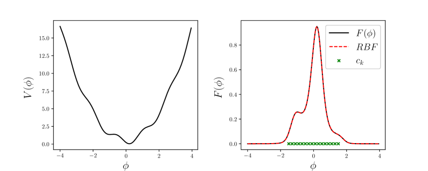
Figure 2: RBF approximation of a test function $F(\phi)=e^{-V(\phi)}$, generated from the potential $V(\phi)=\phi^{2}+\sin^{2}\left(2\phi-0.5\right)$, with fixed Gaussian $A=5$ widths, and a uniformly distributed $c_{k}$ centers.

It can be seen from this simple example that by setting the widths to a constant value and the centers to an interval that covers the range of the $F(\phi)$ function, it is possible to approximate any compact nonlinear function with very good accuracy. It is also worth noting that by an appropriate scaling of the function to a specific interval, the interval of the centers could also be held fixed, with the consequence that the scaling might change the necessary width of the Gaussians, therefore, the determination of good $(A,c_{k})$ parameters is not straightforward, but in practice does not pose any problems. We will come back to this topic later and show that by scaling the fields, a good parameter selection is always possible.

In the next step let us diagonalize the symmetric, circulant $M$ matrix that mixes the field components with its neighbors in coordinate space. To do this we can apply a similarity transformation using a matrix $U$ to get $M=U\Lambda U^{T}$, where $\Lambda$ is now an $N_{t}\times N_{x}$ diagonal matrix, where the diagonal elements will be the eigenvalues of $M$. The $U$ transformation matrix is related to the discrete Fourier transform and can be built from the eigenvectors of $M$. By transforming the $\phi$ vectors with the unitary transformation $U$ as $\widetilde{\Phi}=U^{T}\phi$, the quadratic expression can be rewritten as $\phi^{T}M\phi\rightarrow\widetilde{\Phi}^{T}\Lambda\widetilde{\Phi}$, where $\Lambda=\text{diag}(\lambda_{ij})$. The values of $\lambda_{ij}$ can be given by the eigenvalues of the discretized Laplace operator that appeared due to the kinetic terms in the Lagrangian and can be written as:

$$\lambda_{ij}=4\left[\sin^{2}\left(\frac{p_{i}}{2}\right)+\sin^{2}\left(\frac{p_{j}}{2}\right)\right],$$ (24)

where $p_{i(j)}=2\pi n_{i(j)}/N_{t(x)}$ are the corresponding momenta, while $n_{i(j)}\in(-N_{t(x)}/2,N_{t(x)}/2]$, with $i(j)\in[0,N_{t(x)}-1]$. Note that the eigenvalues of $M$ do not depend on the lattice resolution $a$, because it was separated from the matrix before. Now, let us apply the transformation to the other terms in Eq. 3.1 that were coming from the RBF expansion, where the first purely quadratic term transforms as $\phi^{T}\hat{A}_{k}\phi\rightarrow A\widetilde{\Phi}^{T}\widetilde{\Phi}$, due to the fact that we have assumed a constant $A$ width parameter for the Gaussian kernels. The constant shift $\hat{C}_{k}$ does not transform because it is not coupled to the fields, however, the linear shift will become non-trivial because $\hat{B}_{k}^{T}\phi\rightarrow\hat{B}_{k}^{T}U\widetilde{\Phi}=(U^{T}\hat{B}_{k})^{T}\widetilde{\Phi}$. Therefore, the transformation will mix the $\widetilde{\Phi}$ terms through the $U$ transformation matrix, or, by looking at it another way, transforms the $B_{k}$ parameter vectors. Writing back everything in Eq. 3.1 the path integral becomes:

$$Z\approx\sum_{k\in\{1,\dots,K\}^{N_{t}\times N_{x}}}\hat{a}_{k}\int\mathcal{D}\widetilde{\Phi}\;\exp\left(\frac{1}{2}\widetilde{\Phi}^{T}\Big[\lambda-2A\Big]\widetilde{\Phi}+(U^{T}\hat{B}_{k})^{T}\widetilde{\Phi}-1^{T}\hat{C}_{k}\right),$$ (25)

where $\widetilde{\Phi}$ is the momentum space field vector. This is now in a diagonal form and can be integrated out easily to get:

$$Z\approx\sum_{k\in\{1,\dots,K\}^{N_{t}\times N_{x}}}\hat{a}_{k}\prod_{i,j=0}^{N_{t}-1,N_{x}-1}\left(\frac{2\pi}{\lambda_{ij}+2A}\right)^{1/2}\exp\left(\frac{(U^{T}\hat{B}_{k})_{i,j}^{2}}{2(\lambda_{ij}+2A)}-C_{k_{i,j}}\right),$$ (26)

where $(U^{T}\hat{B}_{k})_{i,j}$ is the $(i,j)$’th element (e.g. in a lexicographic ordering) of the transformed $\hat{B}_{k}$ vector. By substituting back the original parameters: linear weights $a_{k}$, centers $c_{k}$, and widths $b_{k}=A\;(\forall k)$ of the RBF network, the path integral can be written as:

$$Z\approx\sum_{k\in\{1,\dots,K\}^{N_{t}\times N_{x}}}\prod_{i,j=0}^{N_{t}-1,N_{x}-1}a_{k_{i,j}}\left(\frac{2\pi}{\lambda_{ij}+2A}\right)^{1/2}\exp\left(\frac{4A^{2}(U^{T}\hat{c}_{k})_{i,j}^{2}}{2(\lambda_{ij}+2A)}-Ac_{k_{i,j}}^{2}\right),$$ (27)

where $\hat{c}_{k}$ is a vector of the RBF centers corresponding to the $k$’th combination, while $c_{k_{i,j}}$ is one element of this vector.

The path integral in this representation after diagonalization still contains a very large sum of weighted Gaussian path integrals, but now the problem is shifted from the mixing of the field values through the kinetic terms in coordinate space to the mixing of the pre-defined centers of the kernel functions in the linear terms in momentum space. This in itself still makes it impossible to rearrange the path integral into a product of factorized quadratic path integrals. It turns out, however, that by a careful construction of the RBF parameters, the full sum can be approximated by a fully separable model, where the mixing disappears and the full path integral could be written as:

$$Z\rightarrow\prod_{i,j=0}^{N_{t}-1,N_{x}-1}\sum_{k=1}^{K}Q_{k}\Big[\widetilde{\Phi}_{i,j},\lambda_{ij},A,c_{k},a_{k}\Big].$$ (28)

The problematic part that is in the way of achieving this form is the transformed $(U^{T}\hat{c}_{k})$ centers of the Gaussian kernel functions. If we could write this as simply $\hat{c}_{k}$, without the transformation, then the whole expression in Eq… could be written in the form of Eq. 28. In general this is not possible, however, we see that in Eq. 27 the path integral depends on a non-trivial expression of the $A$ parameters, the $\lambda_{ij}$ eigenvalues, and the $c_{k}$ centers, therefore, it could be possible to select such parameters that make the difference between the path integrals, with and without transforming the centers, negligible, while still making it possible to estimate any nonlinear relationship. To quantify this, let us set $a_{k}=1\;(\forall k)$ and define $Z_{0}$ and $Z_{1}$ as follows:

$$Z_{0}(N_{C})=\sum_{k\in\{1,\dots,K\}^{N_{C}}}\prod_{i,j=0}^{N_{t}-1,N_{x}-1}\left(\frac{2\pi}{\lambda_{ij}+2A}\right)^{1/2}\exp\left(\frac{4A^{2}(U^{T}\hat{c}_{k})_{i,j}^{2}}{2(\lambda_{ij}+2A)}-Ac_{k_{i,j}}^{2}\right),$$ (29)

$$Z_{1}(N_{C})=\sum_{k\in\{1,\dots,K\}^{N_{C}}}\prod_{i,j=0}^{N_{t}-1,N_{x}-1}\left(\frac{2\pi}{\lambda_{ij}+2A}\right)^{1/2}\exp\left(\frac{4A^{2}c_{k_{i,j}}^{2}}{2(\lambda_{ij}+2A)}-Ac_{k_{i,j}}^{2}\right),$$ (30)

where $Z_{0}$ is the full expression including the transformed centers, while $Z_{1}$ is the path integral where the centers are not transformed. The $N_{C}$ parameter is the number of terms that we will consider in the summation, which generally should be smaller than all the possible combinations when we choose large $N_{t}$ and $N_{x}$, therefore, to make the calculations numerically tractable, we will consider $N_{C}<K^{N_{t}\times N_{x}}$. Statistically this will not be a problem if we choose large enough $N_{C}$ and use sufficiently enough samples $M$ to make the simulations. This will be clarified in more detail when we define the algorithm to obtain the error distributions.

The task is to compare $Z_{0}$ and $Z_{1}$ for different $c_{k}$ and $A$ parameters and determine the cases where the differences are negligible. Considering the fact that $Z$ in itself is not a meaningful quantity and could take very large or very small values, the necessary quantity that is used to calculate the observables and that we would need to compare is actually $W=\ln Z$, therefore, the error measure we will use is defined as the averaged absolute relative error between the logarithm of $Z_{0}$ and $Z_{1}$:

$$E_{R}(\ln Z)=\frac{1}{M}\sum_{i=1}^{M}\left[\frac{|\ln Z_{0,i}(N_{C})-\ln Z_{1,i}(N_{C})|}{|\ln Z_{0,i}(N_{C})|}\right],$$ (31)

where $M$ is the number of samples, each having $N_{C}$ different randomly generated combinations of the kernels that are defined for fixed centers and widths. To estimate the error in $\ln Z$ that is induced by the unitary transformation, the following steps have been followed:

• Fix the parameters of the RBF network, which include the number of kernels $K$, the width of the Gaussians $A$, and the k-number of centers $c_{k}$. The centers are chosen in a predefined interval $[a,b]$, with some $\Delta c_{k}$ resolution.

• Set the lattice size $N_{t}$ and $N_{x}$, the number of combinations $N_{C}$, and the number of samples $M$.

• Generate $N_{C}$ randomly chosen combinations from all the possibilities. By doing this $M$ times, we can obtain the statistics of the error distributions, where $E_{R}$ is defined as the mean value of the obtained errors in the different samples.

For the first test let us compare the $N_{C}$ dependence of the $E_{R}(\ln Z)$ error in three different scenarios where the parameters are given in Tab. 1. The aim in this simulation is to see how the error evolves with the number of $N_{C}$ combinations and to give a first estimate of the magnitudes of the error when the centers are distributed symmetrically around 0 and in the case when they are not symmetric to 0. The result can be seen in Fig. 3, where some very clear conclusions can be made by examining the errors.

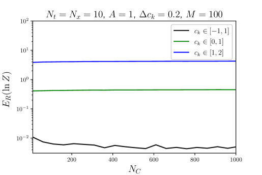
Figure 3: Dependence of the relative error, defined in Eq. 31, on the number of combinations $N_{C}$ for different sets of $c_{k}$ centers for fixed $A=1$ widths. The corresponding parameters of the system and the RBF network are given in Tab. 1.

$M$	$A$	$c_{k}$	$\Delta c_{k}$	$N_{t},N_{x}$
$100$	$1$	$[-1,1]$	$0.2$	$10,10$
$100$	$1$	$[0,1]$	$0.2$	$10,10$
$100$	$1$	$[1,2]$	$0.2$	$10,10$

Table 1: Paramaters for the first test to observe the relative error dependence on the number of combinations $N_{C}$ for three different RBF networks. The corresponding results are shown in Fig. 3.

The most important observation we could make is the difference in the magnitude of the errors for the symmetric and for the non-symmetric cases, where, in the case of symmetric centers, the error is much smaller than in the two other cases. The other observation is that the relative error tends to be saturating after taking a few hundred combinations, which property makes the use of $N_{C}<K^{N_{t}\times N_{x}}$ a sensible choice. The number of combinations that it takes to achieve the saturation depends on the distribution of the specific centers and tends to be larger for smaller centers, where the error also seems to be smaller.

In the second example let us further analyze the $N_{C}$ dependence of the relative errors but now only using symmetric centers, with different width parameters $A$, and with different intervals defined as $c_{k}\in[-A_{c},A_{c}]$, with $K=10$ and $\Delta c_{k}=0.2A_{c}$. The parameters are collected in Tab. 2, while the results are shown in Fig. 4.

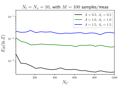
Figure 4: The $N_{C}$ (number of combination) dependence of the relative errors, defined in Eq. 31, for different sets of RBF parameters using only symmetric centers around zero, where $A_{c}$ represents the boundary values of the centers as $c_{k}\in[-A_{c},A_{c}]$. The corresponding parameters are given in Tab. 2.

$M$	$A$	$c_{k}$	$\Delta c_{k}$	$N_{t},N_{x}$
$100$	$0.5$	$[-0.5,0.5]$	$0.1$	$10,10$
$100$	$1$	$[-1,1]$	$0.2$	$10,10$
$100$	$1.5$	$[-1.5,1.5]$	$0.3$	$10,10$

Table 2: Paramaters for the second test to observe the relative error dependence on the number of combinations $N_{C}$ for three different RBF networks using only symmetric $c_{k}$ centers around zero. The corresponding results are shown in Fig. 4.

The results shown in Fig. 4 show the same behavior as what we have observed previously in Fig. 3, where the symmetric center configuration was able to give a very small relative error in the range of a few percentage. The $N_{C}$ dependence also shows the same behavior, where after a few hundred combinations the relative error tends to saturate, therefore, we don’t need to consider all the possible combinations to be able to say something about the error distribution. The important takeaway from the results in Fig. 4 is that the magnitude of the error depends on the distribution of the centers and also on the width of the Gaussian kernels, which is expected as $A$ is also present in $Z_{0}$ and $Z_{1}$.

In Fig. 5 we further analyze the dependence of the relative error on the $A$ and $c_{k}$ parameters, where again only symmetric centers were used with a sensible range given by $[-A_{c},A_{c}]$ with $A_{c}\in[0.5,2]$ and $A\in[0.5,2]$. In these calculations the number of combinations is fixed to $N_{C}=200$, so that a saturation of the relative errors is reached, and we take $M=500$ samples per measurement to get good statistics.

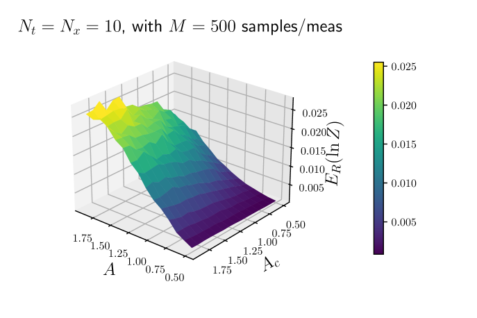
Figure 5: Relative error dependence on the Gaussian width $(A)$ and on the symmetric center boundary $(A_{c})$ parameters, where the centers are defined as $c_{k}\in[-A_{c},A_{c}]$. To reach saturation, $N_{C}=200$ number of combinations were used in each sample, and to get good statistics, $M=500$ samples were used per measurement.

From the results shown on Fig. 5, it can be seen that the relative error stays under a few percent in the intervals that were given. This is a general behavior of the error, and the most important result we can deduce from these simulations is that the relative error in $\ln Z$ stays very low in the case when we use $c_{k}$ centers that are in a well-defined range that is symmetric around zero. The error depends on the width parameters as well, however, for sensible choices the error still stays under a few percent. The actual parameters that are needed to approximate a specific function depend heavily on the function itself, but this function can always be scaled and shifted so that it is centered around zero. This does not change the observables that can be extracted from the path integrals, therefore, selecting a symmetric $c_{k}$ is always possible. Special care might be needed in the case of gauge theories with local symmetries, however, in the case of the interacting scalar fields, it is not a problem. The value of $A$ depends on the shape of the function, e.g., if it’s heavily oscillating, a larger $A$ could be needed. For smooth, non-oscillating functions, choosing $A\in\mathcal{O}(1)$ is a good starting point.

Lastly, let us examine the actual distribution of the errors with a fixed $K=20$ number of kernels, $c_{k}\in[-A_{c},A_{c}]$ centers, and different $A$ and $A_{c}$ intervals shown in Tab. 3. The simulations are done by specifying one $A$ width and one $A_{c}\rightarrow c_{k}\in[-A_{c},A_{c}]$ center (from the previously determined intervals for $A$ and $A_{c}$) at each sample, calculating the errors for these values, and then doing this $M$ times. After we have enough statistics, the histogram of the errors can be obtained. This is also an important quantity, as it is needed when we want to, e.g., calculate the uncertainty of the observables that are calculated with the RBF model. In these simulations the relative errors and the normalized errors defined in Eq. 32 and Eq. 33 are both calculated using $M=10000$ samples to estimate the histograms.

$$E_{rel}=\frac{Z_{0}-Z_{1}}{Z_{0}},$$ (32)

$$E_{normalized}=\frac{Z_{0}-Z_{1}}{\max{\{|Z_{0,i}-Z_{1,i}|_{\forall i}}\}},$$ (33)

where $\max{\{|Z_{0,i}-Z_{1,i}|_{\forall i}}\}$ is the maximum value of the absolute differences, chosen from all of the samples. The normalization in $E_{normalized}$ is used because only the shape of the distribution is important and not the actual value of the difference.

$A$	$A_{c}$	$K$	$N_{t},N_{x}$
$[0.25,2]$	$[0.25,2]$	$20$	$10,10$
$[0.25,5]$	$[0.25,2]$	$20$	$10,10$

Table 3: Parameters used to examine the distributions of the errors defined in Eq. 32 and Eq. 33 for a fixed $A_{c}$ interval and two different $A$ interval sets. The parameter intervals mean that a specific parameter combination is selected from the given intervals in each sample. The corresponding results are shown in Fig. 6.

In Fig. 6 the distribution of the relative error and the normalized difference between $Z_{0}$ and $Z_{1}$ can be seen, showing a clear peak near zero, which is the expected behavior for symmetric centers.

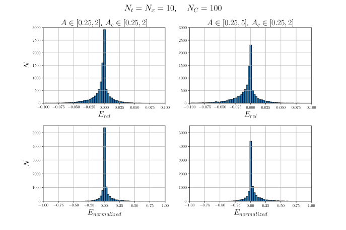
Figure 6: Distributions of the errors defined in Eq. 32 and Eq. 33 using the parameters summarized in Tab. 3. On the upper two plots the distribution of the relative errors is shown, while on the bottom two plots the distribution of the normalized difference is shown.

The distributions also show that for smaller $A$ parameters, the peak near zero is larger, which means that the approximation will be better by using smaller widths for the same symmetric centers.

After observing the behavior of the relative errors under specific parameter sets, we could deduce the following statement for 1+1 dimensions:

• If we set the $c_{k}$ centers to be symmetric around zero, with some corresponding $A$ width parameter, then the path integral can be approximated by a separable form in momentum space that is shown in Eq. 28 with an accuracy of a few percent for $\ln Z$.

The simulations shown here have been done only in 1+1 dimensions, however, the situation does not change in higher dimensions. The actual values of the centers and widths and the corresponding relative errors will change, but the original statement, as the path integral could be approximated by a good accuracy, stays the same.

To summarize the method in 1+1 dimensions, let us write down the steps and the resulting approximation for the path integral in Eq. 3.1:

$$Z\approx\sum_{k\in\{1,\dots,K\}^{N_{t}\times N_{x}}}\hat{a}_{k}\int\mathcal{D}\widetilde{\Phi}\;\exp\left(\frac{1}{2}\widetilde{\Phi}^{T}\Big[\Lambda-2A\Big]\widetilde{\Phi}+(U^{T}\hat{B}_{k})\widetilde{\Phi}-1^{T}\hat{C}_{k}\right)\;\rightarrow\;$$

$$\rightarrow\text{ (choose 'good' $c_{k}$ and $A=b_{k}(\forall k)$, RBF parameters)}\rightarrow$$

$$\rightarrow\sum_{k\in\{1,\dots,K\}^{N_{t}\times N_{x}}}\hat{a}_{k}\int\mathcal{D}\widetilde{\Phi}\;\exp\left(\frac{1}{2}\widetilde{\Phi}^{T}\Big[\Lambda-2A\Big]\widetilde{\Phi}+\hat{B}_{k}\widetilde{\Phi}-1^{T}\hat{C}_{k}\right)\rightarrow$$

$$\rightarrow\prod_{i,j=0}^{N_{t}-1,N_{x}-1}\int d\widetilde{\Phi}_{i,j}\;\left[\sum_{k=1}^{K}a_{k}\exp\Bigg(-\frac{1}{2}\Big[\lambda_{ij}-2A\Big]\widetilde{\Phi}_{i,j}^{2}+2Ac_{k}\widetilde{\Phi}_{i,j}-Ac_{k}^{2}\Bigg)\right],$$ (34)

where the first line shows the large sum of quadratic path integrals in momentum space, while the third line shows its approximation with a ’good’ RBF parametrization. In the fourth line we have rewritten the path integral into a product of small sums that is factorized in the different lattice sites. Using this representation, the integral can be done separately for every lattice site without any mixing between the field values and has the closed-form result as follows:

$$Z\approx\prod_{i,j=0}^{N_{t}-1,N_{x}-1}\left[\sum_{k=1}^{K}a_{k}\left(\frac{2\pi}{\lambda_{ij}+2A}\right)^{1/2}\exp\left(\frac{4A^{2}c_{k}^{2}}{2(\lambda_{ij}+2A)}-Ac_{k}^{2}\right)\right].$$ (35)

Using this approximation, the original $\mathcal{O}(K^{N_{t}\times N_{x}})$ complexity is reduced to $\mathcal{O}(K\times N_{t}\times N_{x})$ when we want to calculate the full path integral. We will see in the next section that due to the factorized form, the situation will be even better when we want to calculate observables.

Before we go into details on how to calculate the observables, two remarks are in order concerning the selection of the centers and the scaling of the fields. Generally the $F[\phi]$ functions that we want to estimate by the RBF network tend to go to zero much faster than the corresponding radial basis functions, therefore, one has to be careful with centers that are far from the dominant parts of the original function, as they could include extra contributions to the path integral in regions that otherwise could have a larger suppression. In practice, it is enough to make sure that the centers are positioned in an interval where the $F[\phi]$ function has dominant contributions. To make sure that we did not include extra contributions, it is advisable to do the calculations with many different parameterizations and compare the results for the observables. Another possible method could be the use of definite integrals of the RBF approximation in a bounded region, where the magnitude of $F[\phi]$ is non-negligible, which could also be expressed in a closed form due to the Gaussian integrals that are involved in the path integral. In this work we will use the former method and express the integrals on an infinite range.

The last remark is about the scaling properties of the fields. By using a simple $\phi\rightarrow S_{c}\phi$ scaling transformation, the function that needs to be approximated on every lattice site also changes as $F[\phi]\rightarrow F[S_{c}\phi]$. In this way $F[\phi]$ can be shaped so that a ’good’ RBF parametrization can be used, therefore, the factorized form in Eq. 28 can be achieved. The scaling also changes the kinetic terms as $\frac{1}{2}\phi^{T}M\phi\rightarrow\frac{1}{2}\phi^{T}(S_{c}^{2}M)\phi$, so the $M$ matrix gets an extra $S_{c}^{2}$ factor, in which case the eigenvalues also change to $\lambda\rightarrow S_{c}^{2}\lambda$. Lastly, the integral measure also gets an extra factor as $d\phi\rightarrow S_{c}d\phi$, so the final result for the integrated path integral can be written as:

$$Z(S_{c})\approx S_{c}\prod_{i,j=0}^{N_{t}-1,N_{x}-1}\left[\sum_{k=1}^{K}a_{k}\left(\frac{2\pi}{S_{c}^{2}\lambda_{ij}+2A}\right)^{1/2}\exp\left(\frac{4A^{2}c_{k}^{2}}{2(S_{c}^{2}\lambda_{ij}+2A)}-Ac_{k}^{2}\right)\right],$$ (36)

where we have accounted for all the extra $S_{c}$ scaling factors. In the next section the method on how to extract some of the necessary observables that are needed to describe, e.g., phase transitions is shown using the RBF approximated path integral formulation.

3.2 Calculating observables

In this section we will show how to extract observables from the radial basis function expansion of the momentum space Euclidean path integrals in 1+1 dimensions that is given by the factorized form shown in Eq. 3.1. One of the most important quantities that can be used to extract observables such as masses of the corresponding particles is the 2-point correlator 38 , or, in other words, the propagator of the dynamical theory. Here, we will derive the expressions for the 2-point ’full’ correlator in momentum space that corresponds to all of the connected and not-connected diagrams. The coordinate space propagators can be derived from the momentum space results by inverse Fourier transform, and the connected propagator in coordinate space can be estimated by subtracting the vacuum expectation values from the coordinate space propagators.

First, let us define a $G(\widetilde{\Phi}_{i,j})$ function of the fields at momentum modes $(i,j)$ as follows:

$$G(\widetilde{\Phi}_{i,j})=\left[\sum_{k=1}^{K}a_{k}\exp\Bigg(-\frac{1}{2}\Big[\lambda_{ij}-2A\Big]\widetilde{\Phi}_{i,j}^{2}+2Ac_{k}\widetilde{\Phi}_{i,j}-Ac_{k}^{2}\Bigg)\right],$$ (37)

where $\widetilde{\Phi}_{i,j}$ is the value of the fields at the discretized momentum modes $(i,j)$, $\lambda_{ij}$ are the eigenvalues of the discretized Laplace operator coming from the kinetic terms, and $a_{k}$, $A$, and $c_{k}$ are the parameters of the radial basis function expansion. The 2-point correlator in 1+1 dimensions is defined as the vacuum expectation value of the product of the fields at momentum modes $(a,b)$ and $(c,d)$ corresponding to momenta $p_{a,b}$ and $p_{c,d}$ and can be written as follows:

$$\langle 0|\widetilde{\Phi}_{a,b}\widetilde{\Phi}_{c,d}|0\rangle=\frac{\prod\limits_{i,j=0}\limits^{N_{t}-1,N_{x}-1}\int d\widetilde{\Phi}_{i,j}\;\widetilde{\Phi}_{a,b}\widetilde{\Phi}_{c,d}\;G(\widetilde{\Phi}_{i,j})}{\prod\limits_{i,j=0}\limits^{N_{t}-1,N_{x}-1}\int d\widetilde{\Phi}_{i,j}\;G(\widetilde{\Phi}_{i,j})},$$ (38)

where the product goes over all of the $N_{t}\times N_{x}$ lattice sites. Without assuming any specific symmetries for fields that come from the underlying theory given by the Lagrangian density, we can separate two different cases, where the integrals will take different forms. In the first case we have $ab=cd$, while in the second case $ab\neq cd$. In the diagonal case the correlator can be given as:

$$\langle 0|\widetilde{\Phi}_{a,b}\widetilde{\Phi}_{c,d}|0\rangle_{ab=cd}=\frac{\Bigg[\int d\widetilde{\Phi}_{a,b}\;\widetilde{\Phi}_{a,b}^{2}\;G(\widetilde{\Phi}_{a,b})\Bigg]\Bigg[\prod\limits_{\begin{subarray}{c}i,j=1\\ ij\neq ab\end{subarray}}\limits^{N_{t},N_{x}}\int d\widetilde{\Phi}_{i,j}\;G(\widetilde{\Phi}_{i,j})\Bigg]}{\prod\limits_{i,j=0}\limits^{N_{t}-1,N_{x}-1}\int d\widetilde{\Phi}_{i,j}\;G(\widetilde{\Phi}_{i,j})}=$$

$$=\frac{\int d\widetilde{\Phi}_{a,b}\;\widetilde{\Phi}_{a,b}^{2}G(\widetilde{\Phi}_{a,b})}{\int d\widetilde{\Phi}_{a,b}\;G(\widetilde{\Phi}_{a,b})}=\frac{\sum\limits_{k=1}\limits^{K}a_{k}\sqrt{2\pi}\exp\left(\frac{4A^{2}c_{k}^{2}}{2(\lambda_{ab}+2A)}-Ac_{k}^{2}\right)\left(\frac{\lambda_{ab}+2A+4A^{2}c_{k}^{2}}{(\lambda_{ab}+2A)^{5/2}}\right)}{\sum\limits_{k=1}\limits^{K}a_{k}\left(\frac{2\pi}{\lambda_{ab}+2A}\right)^{1/2}\exp\left(\frac{4A^{2}c_{k}^{2}}{2(\lambda_{ab}+2A)}-Ac_{k}^{2}\right)}$$ (39)

where we have seen that due to the factorized form of the radial basis function approximation, many of the terms where $(i,j)\neq(a,b)$ can be factorized out with the normalization, therefore, we will have a very simple closed-form expression for the diagonal elements of the 2-point correlators in momentum space.

The off-diagonal elements can be expressed the same way, however, in this case, two separate terms remain in the product for the different lattice sites:

$$\langle 0|\widetilde{\Phi}_{a,b}\widetilde{\Phi}_{c,d}|0\rangle_{ab\neq cd}\!\! = \!\!\frac{\Bigg[\int d\widetilde{\Phi}_{a,b}\;\widetilde{\Phi}_{a,b}G(\widetilde{\Phi}_{a,b})\Bigg]\Bigg[\int d\widetilde{\Phi}_{c,d}\;\widetilde{\Phi}_{c,d}G(\widetilde{\Phi}_{c,d})\Bigg]\Bigg[\prod\limits_{\begin{subarray}{c}i,j=1\\ ij\neq ab\\ ij\neq cd\end{subarray}}\limits^{N_{t},N_{x}}\int d\widetilde{\Phi}_{i,j}\;G(\widetilde{\Phi}_{i,j})\Bigg]}{\prod\limits_{i,j=0}\limits^{N_{t}-1,N_{x}-1}\int d\widetilde{\Phi}_{i,j}\;G(\widetilde{\Phi}_{i,j})}$$ (40)

$$= \frac{\Big[\int d\widetilde{\Phi}_{a,b}\;\widetilde{\Phi}_{a,b}G(\widetilde{\Phi}_{a,b})\Big]\Big[\int d\widetilde{\Phi}_{c,d}\;\widetilde{\Phi}_{c,d}G(\widetilde{\Phi}_{c,d})\Big]}{\Big[\int d\widetilde{\Phi}_{a,b}\;G(\widetilde{\Phi}_{a,b})\Big]\Big[\int d\widetilde{\Phi}_{c,d}\;G(\widetilde{\Phi}_{c,d})\Big]},$$

where $\int d\widetilde{\Phi}_{i,j}\;\widetilde{\Phi}_{i,j}G(\widetilde{\Phi}_{i,j})$ does not vanish automatically due to the field shifts, and generally can be given as:

$$\int d\widetilde{\Phi}_{a,b}\;\widetilde{\Phi}_{a,b}G(\widetilde{\Phi}_{a,b})=\sum\limits_{k=1}\limits^{K}a_{k}\left(\frac{2\pi}{\lambda_{ij}+2A}\right)^{1/2}\exp\left(\frac{4A^{2}c_{k}^{2}}{2(\lambda_{ij}+2A)}-Ac_{k}^{2}\right).$$ (41)

To summarize, in the diagonal case we have a sum of $K$ exponential terms, while in the non-diagonal case we will be left with a sum of $K^{2}$ exponential terms both in the numerator and in the denominator. In Sec. 4.2 we will show how to extract the masses from the momentum space 2-point correlators in the case of the real scalar $\phi^{4}$ theory.

The second observable that can be easily calculated from the model is the total quantum fluctuations that can be defined through the mass squared derivative of the logarithm of the partition function as:

$$-\frac{1}{V}\frac{\partial\ln Z}{\partial m^{2}}=\langle\phi^{2}\rangle=\int\frac{d^{D}p}{(2\pi)^{D}}\langle|\widetilde{\Phi}(p)|^{2}\rangle$$ (42)

where $V$ is the total volume and $m$ is the mass parameter in the Lagrangian density. The total fluctuation in 1+1 dimensions in discretized space-time with $N_{t},N_{x}$ number of temporal and spatial lattice points, with $\Delta t=\Delta x=1$, can be given as:

$$\langle\phi^{2}\rangle\approx\frac{1}{N_{t}N_{x}}\sum_{i,j=0}^{N_{t}-1,N_{x}-1}\langle 0|\widetilde{\Phi}_{i,j}^{2}|0\rangle,$$ (43)

where we have to average over the momentum space fluctuations at different $(i,j)$ momentum modes. Using the radial basis model, the total fluctuations can be expressed by using the results for the diagonal part of the 2-point correlators and have the simple form of:

$$\langle\phi^{2}\rangle\approx\frac{1}{N_{t}N_{x}}\sum_{i,j=1}^{N_{t},N_{x}}\left(\frac{\sum\limits_{k=1}\limits^{K}a_{k}\sqrt{2\pi}\exp\left(\frac{4A^{2}c_{k}^{2}}{2(\lambda_{ij}+2A)}-Ac_{k}^{2}\right)\left(\frac{\lambda_{ij}+2A+4A^{2}c_{k}^{2}}{(\lambda_{ij}+2A)^{5/2}}\right)}{\sum\limits_{k=1}\limits^{K}a_{k}\left(\frac{2\pi}{\lambda_{ij}+2A}\right)^{1/2}\exp\left(\frac{4A^{2}c_{k}^{2}}{2(\lambda_{ab}+2A)}-Ac_{k}^{2}\right)}\right),$$ (44)

which form has to give back the same result if one calculates it purely from the logarithm of $Z$ by taking the derivative of $m^{2}$ and dividing by the volume.

The third observable we will consider is the vacuum expectation value of the fields at $x$ that can be defined as the inverse Fourier transform of the one-field insertions in momentum space as:

$$\langle\phi(x)\rangle=\int\frac{d^{D}p}{(2\pi)^{D}}\;e^{-ipx}\langle\widetilde{\Phi}(p)\rangle,$$ (45)

where in 1+1 dimensions the $\langle\widetilde{\Phi}(p)\rangle$ expectation value can be given in the following closed form:

$$\langle\widetilde{\Phi}(p)\rangle\rightarrow\langle 0|\widetilde{\Phi}_{a,b}|0\rangle=\frac{\int d\widetilde{\Phi}_{a,b}\;\widetilde{\Phi}_{a,b}\;G(\widetilde{\Phi}_{a,b})\prod\limits_{\begin{subarray}{c}i,j=0\\ i,j\neq a,b\end{subarray}}\limits^{N_{t}-1,N_{x}-1}\int d\widetilde{\Phi}_{i,j}\;G(\widetilde{\Phi}_{i,j})}{\prod\limits_{i,j=0}\limits^{N_{t}-1,N_{x}-1}\int d\widetilde{\Phi}_{i,j}\;G(\widetilde{\Phi}_{i,j})}=$$

$$=\frac{\sum\limits_{k=1}\limits^{K}a_{k}\sqrt{2\pi}\exp\left(\frac{4A^{2}c_{k}^{2}}{2(\lambda_{ab}+2A)}-Ac_{k}^{2}\right)\left(\frac{4A^{2}c_{k}^{2}}{(\lambda_{ab}+2A)^{3/2}}\right)}{\sum\limits_{k=1}\limits^{K}a_{k}\left(\frac{2\pi}{\lambda_{ab}+2A}\right)^{1/2}\exp\left(\frac{4A^{2}c_{k}^{2}}{2(\lambda_{ab}+2A)}-Ac_{k}^{2}\right)},$$ (46)

where $a,b$ represents one momentum component of the fields. The vacuum expectation value of the field configurations is one of the most important quantities in studying phase transitions, due to its relation to the magnetization, which is defined through the coordinate space average of $\langle\phi(x)\rangle$, and is an order parameter of the spontaneous symmetry breaking in interacting scalar field theories, or discrete magnetic systems 45 .

Using the same analogy, other observables can be calculated by the same method using the factorized form of the radial basis function approximated path integral. In the next section a simple example will be shown for the free real scalar field theory in 1+1 dimensions.

3.3 Example: the free scalar field in 1+1 dimensions

The non-interacting real scalar field theory in 1+1 dimensions is the simplest system where the method could be easily followed. The calculation for more complex theories with, e.g., nonlinear interactions and/or higher dimensions follows the same procedure. On a sidenote, in the case of gauge theories, or theories including Grassman variables, e.g., for fermionic fields, the method needs to be extended due to the different kinetic terms and different symmetries, which will be the main topic of some future works.

In this section we will show the working principles of the method by using three different parameterizations of the RBF networks and also including one instance where the field is scaled to a smaller interval using $S_{c}>1$. For now, staying with the problem at hand, the Lagrangian density for the free scalar field with mass $m$ can be written as:

$$\mathcal{L}=\frac{1}{2}\partial_{\mu}\phi(x)\,\partial^{\mu}\phi(x)+\frac{m^{2}}{2}\phi(x)^{2},$$ (47)

where $m$ is the mass, and $x$ represents the space-time coordinates. By discretizing the Lagrangian density in 1+1 dimensions, assuming periodic boundary conditions, and setting $\Delta t=\Delta x=a$, the action integral can be cast in a discretized sum as:

$$S=\sum_{i,j=0}^{N_{t}-1,N_{x}-1}\Bigg(S_{c}^{2}\frac{\left(\phi_{i+1,j}-\phi_{i,j}\right)^{2}+\left(\phi_{i,j+1}-\phi_{i,j}\right)^{2}}{2}+S_{c}^{2}\frac{(am)^{2}}{2}\phi_{i,j}^{2}\Bigg),$$ (48)

where we have also applied a field scaling as $\phi\rightarrow S_{c}\phi$. In the calculations, we will set $a=1$ and $m=1$, however, we keep their dependence during the derivation for clarity.

In the next step let us separate the kinetic term from the static quadratic mass terms and define the $F(\phi_{i,j})$ function that has to be approximated by the RBF network as follows:

$$F(\phi_{i,j})=\exp\left(-S_{c}^{2}\frac{(am)^{2}}{2}\phi_{i,j}^{2}\right),$$ (49)

where we have kept the dependence on the $S_{c}$ scaling and on the $a$ lattice resolution. In order to show that different ’good’ parametrizations will give the same results, we have done the calculations using three different RBF networks with the parameters shown in Tab. 4.

In all cases we have assumed $m=1$, in which case the $F(\phi)$ function will be dominant in the range of $\phi\in[-4,4]$. In the first parametrization we have applied a scaling of $S_{c}=4$, which scales the function into the new range of $\phi^{*}\in[-1,1]$. This makes it possible to use smaller centers near zero in the account of a possibly larger $A$ Gaussian width parameter. In the second case no scaling was applied for the fields with uniformly distributed centers around zero. In this case a smaller $A$ parameter could be used due to the larger interval that $F[\phi]$ covers. In the third case, similar to the second one, no scaling was applied, however, here the centers have been chosen randomly and not distributed uniformly around zero. Note that in all cases the $c_{k}=0$ center is omitted. By doing this, we force the network to try to estimate the nonlinear function with a set of shifted Gaussians, with different, non-zero weights in each case. The results can be seen in Fig. 7, where the RBF approximation of the $F(\phi)$ functions and the ’trained’ $a_{k}$ parameters are also shown for the three different parameterizations.

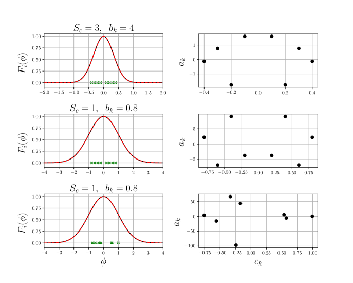
Figure 7: RBF approximation of the $F(\phi)$ function that is defined in Eq. 49 for the free scalar field case. The left-hand side plots show the (scaled) $F(\phi)$ functions with the corresponding RBF approximations and the positions of the RBF centers, while the right-hand side plots show the fitted $a_{k}$ RBF weights for each case.

$S_{c}$	$c_{k}$	$A$	$N_{t},N_{x}$	$m$
$3$	$[-0.4,-0.3,-0.2,-0.1,0.1,0.2,0.3,0.4]$	$4$	$40,40$	$1$
$1$	$[-0.8,-0.6,-0.4,-0.3,0.3,0.4,0.6,0.8]$	$0.8$	$40,40$	$1$
$1$	$[-0.75,-0.56,-0.33,-0.24,-0.17,0.53,0.57,0.99]$	$0.8$	$40,40$	$1$

Table 4: Three different parameterizations of the RBF networks and the corresponding system parameters for describing the lattice-regularized free scalar field theory in 1+1 dimensions.

Using the fitted parameters $a_{k}$, $c_{k}$, and $A$, the momentum space correlator given by Eq. 3.2 and Eq. 40 can be calculated in a closed form. In addition, the scaling introduces an $S_{c}^{2}$ factor outside of the correlator due to the two field insertions, while $\lambda_{ij}\rightarrow S_{c}^{2}\lambda_{ij}$ changes due to the scaled kinetic part. The momentum space correlator thus can be given as:

$$\widetilde{C}(p_{t},p_{x};q_{t},q_{x})=S_{c}^{2}\langle 0|\widetilde{\Phi}_{p_{t},p_{x}}\widetilde{\Phi}_{q_{t},q_{x}}|0\rangle_{\lambda\rightarrow S_{c}^{2}\lambda},$$ (50)

where $p_{t},p_{x},q_{t},q_{x}$ are the corresponding momenta, where the correlator is evaluated. To get the coordinate space correlator, the inverse Fourier transform has to be applied to the momentum space correlator as:

$$C(n_{t},n_{x};m_{t},m_{x})=\frac{1}{(N_{t}a)(N_{x}a)}\sum_{p_{t},p_{x},q_{t},q_{x}}e^{2\pi i\left(\frac{p_{t}n_{t}+q_{t}m_{t}}{N_{t}}+\frac{p_{x}n_{x}+q_{x}m_{x}}{N_{x}}\right)}\widetilde{C}(p_{t},p_{x};q_{t},q_{x}),$$ (51)

where due to translational symmetry it is sufficient to fix the initial coordinates $m_{t}$ and $m_{x}$ to $0$. The exact solution for the coordinate space correlator in 1+1 dimensions can be given by the modified Bessel function of the second kind as 51 :

$$C_{true}(r)=\frac{1}{2\pi}K_{1}(mr),$$ (52)

where the distance on the lattice is defined as $r=\sqrt{(n_{x}a-m_{x}a)^{2}+(n_{t}a-m_{t}a)^{2}}$, while $K_{1}(mr)$ is the modified Bessel function of the second kind. In Fig. 8 the true correlator is compared to the model results after inverse Fourier transforming the momentum space expressions, showing a very good match in all cases.

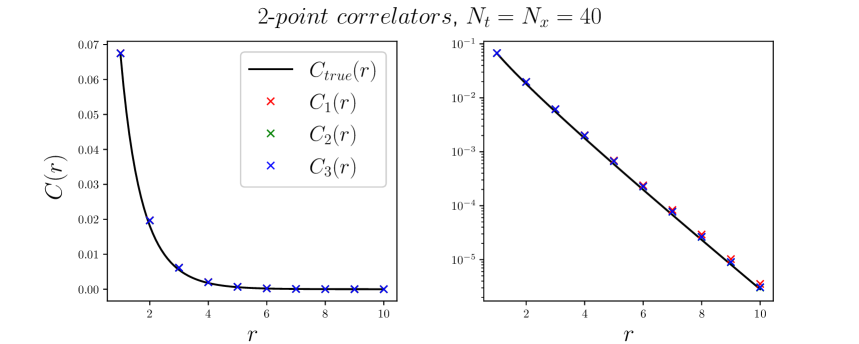
Figure 8: The true and RBF approximated 2-point correlators in position space for the three different RBF network parametrizations are shown in linear (left) and logarithmic (right) scales.

From the results shown here we have seen that the true correlator can be reproduced with very good accuracy using the RBF approximated momentum space correlators. The actual parameters of the RBF kernels can be varied according to the function that has to be approximated, and the most important condition that has to be satisfied is that the centers have to be distributed around zero. By scaling the fields, the RBF parameters can be fine-tuned so that a ’good’ parametrization can be used.

In the next section the interacting $\phi^{4}$ theory will be addressed by calculating the bare parameter dependence of the renormalized masses in the unbroken phase and by determining the phase transition line that separates the broken and unbroken phases.

4 $\phi^{4}$ theory in 1+1 dimensions

4.1 Interacting real scalar fields

The interacting scalar $\phi^{4}$ theory is one of the simplest quantum field theories, where the nonperturbative effects arising from the quartic self-interactions can be analyzed in a relatively simple manner. Despite its simple form, the nonlinear quartic self-interaction makes it possible to study phase transitions, critical phenomena, and spontaneous symmetry breaking and can serve as a prototype model to understand more complex systems, e.g., in condensed matter physics, cosmology, or the standard model 53 ; 54 . In this section the RBF model will be applied to the 1+1 dimensional real scalar $\phi^{4}$ theory and show that it is capable of describing the discretized system with an accuracy compared to previous lattice results.

The calculations that will be shown here do not aim to give a full, comprehensive description of the system (e.g., the continuum limit is not considered, or no finite size scaling is examined), but they are aimed at showing that the method is able to calculate the necessary observables to describe renormalized parameters and phase transitions. Due to the well-defined form of the RBF approximation, these extensions, e.g., taking the continuum limit, should not pose any problems and could be done by using the same techniques as it is done, for example, in lattice methods 55 . One of the main advantages of the RBF method in comparison to lattice Monte Carlo methods is that the calculations can be done very fast, e.g., obtaining the phase transition line for multiple parameter combinations only takes a few seconds on a standard notebook, which would otherwise take at least many hours or even days with lattice Monte Carlo methods. The other advantages and future prospects of the RBF model will be summarized in Sec. 5.

In the D-dimensional continuum theory, the (Euclidean) action integral of the interacting $\phi^{4}$ model can be written in the following simple form:

$$S=\int d^{D}x\;\left(\frac{1}{2}\partial_{\mu}\phi(x)\,\partial^{\mu}\phi(x)+\frac{m_{0}^{2}}{2}\phi(x)^{2}+\frac{\lambda_{0}}{4!}\phi(x)^{4}\right),$$ (53)

where $m_{0}$ represents the bare mass, while $\lambda_{0}$ is the bare coupling that controls the strength of the quartic self-interaction. The discretized model in 1+1 dimensions on an $N_{t}\times N_{x}$ lattice with lattice resolution $a$ can be written as:

$$S=\!\!\!\sum_{i,j=0}^{N_{t}-1,N_{x}-1}\Bigg(S_{c}^{2}\frac{\left(\phi_{i+1,j}-\phi_{i,j}\right)^{2}+\left(\phi_{i,j+1}-\phi_{i,j}\right)^{2}}{2}+S_{c}^{2}\frac{(am_{0})^{2}}{2}\phi_{i,j}^{2}+S_{c}^{4}\frac{(a^{2}\lambda_{0})}{4!}\phi_{i,j}^{4}\Bigg),$$ (54)

where $S_{c}$ acts as a field scaling parameter $\phi_{i,j}\rightarrow S_{c}\phi_{i,j}$ as before. The discretized action defined like this now depends on the dimensionless $(am_{0})^{2}$ and $(a^{2}\lambda_{0})$ parameters, where both $m_{0}^{2}$ and $\lambda_{0}$ have dimensions of mass squared.

In this work we only consider the lattice-regularized theory with finite $a$, and will not take the continuum limit that is otherwise needed to compare the calculations to experimental results. As the RBF method described here is based on the discretized path integral formulation, taking the continuum limit can be done with the same techniques that it is usually done in lattice Monte Carlo methods. This would require a careful extrapolation and the calculation of the observables using different (decreasing) lattice spacings by keeping some corresponding parameter combinations fixed. One of the main difficulties using lattice Monte Carlo methods is the very long time that it takes to do the simulations at small lattice spacings, therefore, usually only a few different combinations are examined and then extrapolated to $a=0$. In some future works we aim to address this issue as well, but for now we will stay with the lattice regularized theory with finite $a$ to be able to compare our results to the Monte Carlo calculations that will be shown in Sec. 4.3.

In this discretized setting, the function that has to be approximated by the RBF network can be written as follows:

$$F(\phi_{i,j})=\exp\left(-S_{c}^{2}\frac{(am_{0})^{2}}{2}\phi_{i,j}^{2}-S_{c}^{4}\frac{(a^{2}\lambda_{0})}{4!}\phi_{i,j}^{4}\right),$$ (55)

where the $S_{c}$ field scaling is also included in the description.

In the calculations that will be shown here, we have set the lattice spacing to $a=1$ and the lattice size to $N_{t}=N_{x}=100$. These parameters will be sufficient to extract the necessary observables we are interested in, where first we will give a description on how to extract the renormalized masses from the momentum space correlators, then a simple example will be given in the non-broken phase where the previously described observables in Sec. 3.2 are calculated. In the case of examining the symmetry breaking and phase transitions, the method we will use to find the critical points in Sec. 4.3 assumes taking the infinite volume limit, which will be straightforward to do in the case of the observables we will use to describe the phase transition line.

4.2 Renormalized mass in the unbroken phase

In the interacting $\phi^{4}$ theory, the corrections in the self-energy that are induced by the nonlinear interactions will modify the locations of the poles in the propagator, thus corresponding to a finite mass shift that depends on the strength of the coupling and corresponds to the physical mass of the theory 58 . Similarly, the coupling constant gets renormalized due to the loop corrections in the four-point function, which alters the strength of the self-interactions, while additionally, in the full ’dressed’ theory, the field itself is also renormalized so that the theory respects the correct normalization and unitarity of the system. Here, we will only consider extracting the renormalized masses, but the field renormalization constant $Z_{R}$ and the renormalization of the coupling constant are also straightforward.

The general method to extract the physical masses in Monte Carlo lattice simulations is to use the connected 2-point correlators in coordinate space, in which case the slope of the exponential decay of the correlator at large Euclidean times corresponds to the physical masses. Due to the fact that the RBF model is defined in momentum space, it is more suitable to use the momentum space correlators to extract the renormalized masses. In the following, let us consider the unbroken phase of the theory where the vacuum expectation value is zero, therefore, the full propagator can be used instead of the connected propagator. The general expression for the momentum space propagator of the full theory near $p^{2}\approx 0$ can be written in the following simple form:

$$\widetilde{G}(p^{2})_{p^{2}\approx 0}\sim\frac{Z_{R}}{p^{2}+m_{R}^{2}},$$ (56)

where $Z_{R}$ is the field renormalization constant, $p^{2}$ corresponds to the physical momenta, while $m_{R}$ represents the renormalized (physical) mass that includes the bare mass plus the finite mass shift as $m_{R}^{2}=m_{0}^{2}+\Sigma$. By inverting the expression in Eq.56 and taking its derivative with respect to $p^{2}$ at $p^{2}=0$, the field renormalization constant can be expressed as a function of the renormalized mass and the derivative of the momentum space correlator. Putting the resulting expression back into the correlator, the renormalized mass can be given by using the value of the correlator at $p^{2}=0$ and the value of its derivative at $p^{2}=0$. The method can be summarized as follows:

$$\widetilde{G}(p^{2})\;\;\rightarrow\;\;\widetilde{G}^{-1}(p^{2})\;\;\rightarrow\;\;Z_{R}=\frac{d\widetilde{G}^{-1}(p^{2})}{dp^{2}}\Bigg|_{p^{2}=0}\;\;\rightarrow\;\;m_{R}^{2}=\frac{Z_{R}}{G^{-1}(p^{2}=0)},$$ (57)

where $\widetilde{G}^{-1}(p^{2})$ is the inverse of the momentum space propagator, $Z_{R}$ is the field renormalization constant, and $m_{R}$ is the renormalized mass.

In this section we would like to examine the behaviour of the renormalized masses for varying coupling strengths at fixed bare mass parameters in the unbroken phase when $m_{0}^{2}>0$. From perturbation theory, and from lattice Monte Carlo simulations 61 one would expect a monotonic increase of the renormalized masses with increasing couplings, however in the strong coupling regime, due to the severe nonperturbative effects, the exact functional form is not straightforward to see. In the following calculations we have fixed the lattice parameters to $N_{x}=N_{t}=100$, with $a=1$ lattice spacing in both direction. The calculations have been made for $(am_{0})^{2}=1$, and $(am_{0}^{2})=4$ in the coupling range of $(a^{2}\lambda_{0})\in[0,50]$, where the renormalized masses have been extracted from the momentum space propagators by using the method described in Eq. 57. As we only want to examine the general behaviour of the renormalized masses (and they relation to each other) and not its absolute values, we have scaled the obtained $m_{R}$ results to lie between $0$ and $1$ in the specified coupling range, as follows:

$$m_{R}^{N}=\frac{m_{R}(\hat{m}^{2},\hat{\lambda})-m_{R}(\hat{m}^{2},\hat{\lambda}=0)}{\max\{m_{R}(\hat{m}^{2},\hat{\lambda})-m_{R}(\hat{m}^{2},\hat{\lambda}=0)\}},$$ (58)

where we have defined the dimensionless $\hat{m}^{2}=(am_{0})^{2}$, and $\hat{\lambda}=a^{2}\lambda_{0}$ parameters. The normalization by $m_{R}(\hat{m}^{2},\hat{\lambda})-m_{R}(\hat{m}^{2},\hat{\lambda}=0)$ makes sure that all of the renormalized masses are between $0$ and $1$, while the shift by $m_{R}(\hat{m}^{2},\hat{\lambda}=0)$ (that corresponds to $\hat{m}$) makes sure that both funtion starts from $0$. According to this, $m_{R}^{N}$ is essentially just the normalized mass shift, which makes it possible to simply compare the coupling dependence of the nonperturbative effects in the case of $\hat{m}^{2}=1$, and $\hat{m}^{2}=4$.

In Fig. 9 the results for the $\hat{\lambda}$ dependent $m_{R}(\hat{m},\hat{\lambda})$ renormalized masses at fixed $\hat{m}^{2}=(am_{0})^{2}$ bare mass parameters can be seen, showing the expected monotonic increasing behaviour with the coupling strength. The comparison also suggest that the magnitude of the mass shift depends on the bare mass and tends to be lower in the case of a larger $\hat{m}$.

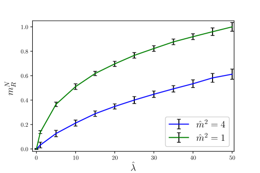
Figure 9: The scaled renormalized mass $m_{R}^{N}$ dependence on the bare parameters $\hat{m}^{2}=(am_{0})^{2}$ and $\hat{\lambda}=(a^{2}\lambda_{0})$ in the interacting $\phi^{4}$ theory using $a=1$ lattice spacing on a $N_{t}\times N_{x}=100\times 100$ lattice, calculated by the RBF approximated path integral formulation.

In these calculations the uncertainty is estimated by calculating the renormalized masses using different RBF parametrizations and $S_{c}$ field scalings, then, from the distribution of the extracted masses, we took the mean values and the corresponding standard deviations to represent the results. Using a large lattice size $N_{t}=N_{x}=100$, the resolution in momentum space will be sufficient enough to give a good estimation of the derivative of the inverse propagator at $p^{2}=0$. From the results it can be seen that the mass gets finite corrections in both cases due to the nonlinear self-interactions of the scalar fields, and as we go up to larger bare mass parameters the mass correction tends to be smaller at fixed couplings.

4.3 Phase transition

In this section the spontaneous symmetry breaking of the interacting $\phi^{4}$ theory will be addressed, and the phase transition line that separates the broken and unbroken phases will be determined by the RBF method in a wide range of couplings. The Lagrangian of the model, with positive mass squared $m_{0}^{2}\geq 0$ and positive coupling $\lambda_{0}>0$, suggests that the system is in the unbroken phase, where the positive coupling makes sure that the potential is bounded from below, which is necessary for stability. The system in this phase possesses a global $\mathbb{Z}_{2}$ symmetry, and the corresponding potential has a stable global minimum at zero vacuum expectation value. In the case of a negative mass squared $m_{0}^{2}<0$ and positive coupling $\lambda>0$, the system undergoes spontaneous symmetry breaking, in which case the vacuum state no longer respects the original $\mathbb{Z}_{2}$ symmetry of the Lagrangian. Instead of a single global minimum at the origin, the potential develops a set of new minima away from zero, which leads to non-zero vacuum expectation values for the field, that is a general sign of the spontaneously broken symmetry P1 .

In this state the system settles into one of the minima, thus selecting a specific vacuum state that breaks the symmetry of the original theory. Due to field fluctuations and finite mass shifts, the phase transition does not happen strictly when $m_{0}^{2}$ becomes negative, and without precise numerical methods that could tackle the nonperturbative regions (e.g., in the strong coupling limit), it is not straightforward to see what would be the critical points where the phase transition occurs. One usual way on how the transition point is searched for in, e.g., lattice techniques is to examine the behavior of the renormalized masses with the change of the coupling P2 . A general sign in this case would be the fast decrease of the mass at the critical coupling. Another signal that is usually searched for is the point where the vacuum expectation value of the fields becomes finite, which signals that the system settles into one of the new vacuum states. This, however, is not always trivial to do without any extra steps, because in the $\phi^{4}$ theory the new vacuum state is also symmetric, therefore, taking the expectation value averages out the fluctuations to zero P3 . There are several methods that exist on how to handle this issue on the lattice, e.g., by introducing an explicit breaking of the symmetry, thus forcing the system to jump into one of the minima, or by a careful construction of how the vacuum expectation value is taken 61 . Here, we will use a different technique based on the effective potential approach that is more suitable for the RBF model.

To define the effective potential, first we have to define the effective action, that is, the quantum-corrected version of the classical action and serves as a generating functional for the one-particle irreducible correlation functions of the theory P4 . First, let us assume an $x$-dependent source term $J(x)$ and define the classical field $\phi_{c}$ that is probed by the background source term as follows:

$$\phi_{c}\equiv\frac{\delta W[J]}{\delta J(x)},$$ (59)

where $W[J]=\ln Z[J]$ is the generating functional of the connected correlators, while $Z[J]$ is defined in Eq. 1. The effective action that governs the quantum-corrected dynamics of the classical field $\phi_{c}$ can be defined using the Legendre transform of the $W[J]$ functional as:

$$\Gamma[\phi_{c}]=W[J]-\int d^{D}x\;J(x)\phi_{c}(x),$$ (60)

where $\Gamma[\phi_{c}]$ is understood as the functional of the classical field configurations. The effective potential P5 captures the quantum corrections to the classical potential and can be given using the effective action by assuming a constant background field $J$. This ’static’ part of the effective action does not govern any dynamics and is useful to extract the vacuum structure and to determine the true vacuum of the theory by minimizing $V_{eff}(\phi)$. By probing the system with a set of different $J$ background fields, the vacuum expectation value of the field will be a function of $J$. By inverting this relation, the effective potential can be expressed as follows:

$$V_{eff}(\phi)\propto\int_{0}^{\phi}d\langle\phi\rangle\;J(\langle\phi\rangle),$$ (61)

where the background field $J$ is understood as a function of the vacuum expectation value of the fields, while due to the constant background field, $\langle\phi\rangle$ can be calculated by taking the derivative of the generating functional with respect to the field shift as:

$$\langle\phi\rangle_{J_{0}}=\frac{\delta\ln Z[J]}{\delta J}\Big|_{J=J_{0}},$$ (62)

where $Z$ is given by the RBF expansion of the partition function defined in Eq. 3.1.

The method we will follow starts by calculating the $J$ dependence of the vacuum expectation of the averaged fields $\langle\phi\rangle_{J}$ for a range of $J$ background fields. To do this, let us define the shifted $F(\phi_{i,j},J)$ function as:

$$F(\phi_{i,j},J)=\exp\left(-S_{c}^{2}\frac{(am_{0})^{2}}{2}\phi_{i,j}^{2}-S_{c}^{4}\frac{(a^{2}\lambda_{0})}{4!}\phi_{i,j}^{4}+JS_{c}\phi_{i,j}\right),$$ (63)

where $J$ is a constant that represents the background field, and the corresponding extra $J\phi_{i,j}$ term is also scaled by $S_{c}$ due to the field scaling. Note that we did not necessarily have to include the $J\phi$ shift in the $F(\phi,J)$ function, because this extra linear does not complicate the path integral in itself. In the case when we do not include it, then the shift will appear as an extra $+J$ term in the linear part in Eq. 3.1 as: $(2Ac_{k})\widetilde{\Phi}\rightarrow(2Ac_{k}+J)\widetilde{\Phi}$.

In this approach, by calculating $\langle\phi\rangle_{J}$ for a set of $J$ fields, we can determine the $J(\langle\phi\rangle)$ from which the effective potential $V_{eff}$ could be determined. This method, however, is not that straightforward due to the properties of the Legendre transform, which requires convexity from the functions involved P6 ; P7 . If the potential is a non-convex function, then the Legendre transform will correspond to its convex hull, which will be the case in the broken phase, where the potential includes many local minima and is a non-convex function of $\phi$. The arising problem due to the non-convexity in the broken phase is addressed, e.g., in P8 , where it is indicated that the effective potential that can be obtained by lattice Monte Carlo simulations correspond to the Maxwell-construction between its saddle-points. In practice this will correspond to straight lines that connect the local minima of the potentials, thus making the effective potential a convex function of $\langle\phi\rangle$. The same behavior is also described in P9 for a more general case, to study of first- and second-order phase transitions.

The results shown here will have the same behavior for the lattice-regularized $\phi^{4}$ theory, therefore, we need a prescription on how to handle this issue. One way would be to identify the end points of the linear parts that correspond to the ’Maxwell construction’ and extract the corresponding vacuum expectation values. This is, however, not the most precise way to do so, because of the uncertainties of the results that could distort the obtained points near $J=0$, which would be necessary to know with very good accuracy. A better and more robust method is to make a simple Ansatz for the effective potential as follows P10 :

$$V_{eff}(\langle\phi\rangle)=\hat{A}(m_{R},Z_{R})\langle\phi\rangle^{2}+\hat{B}(\lambda_{R},Z_{R})\langle\phi\rangle^{4},$$ (64)

where the $A(m_{R},Z_{R})$ parameter depends on the renormalized mass $m_{R}$ and the field renormalization constant $Z_{R}$, while the $B(\lambda_{R},Z_{R})$ parameter also depends on the renormalized coupling $\lambda_{R}$. In a more general case, higher order and logarithmic terms could also be included in the effective potential, however, in this case, this simple functional form is enough, especially in the large $J$ region where we are mostly interested in. Using this general form for the effective potential makes it possible to make a robust fit to the whole range of the obtained $J(\langle\phi\rangle)$ points through the following parametrization:

$$J(\langle\phi\rangle)=a\langle\phi\rangle^{3}+b\langle\phi\rangle\;\;\rightarrow\;\;\begin{cases}\hat{A}(m_{R},Z_{R})=b/2\\ \hat{B}(\lambda_{R},Z_{R})=a/4\end{cases}$$ (65)

in which case the minima of the potential can be expressed using the fitted $(a,b)$ parameters as:

$$\langle\phi\rangle_{min}=\begin{cases}0,&b\geq 0\\ \pm\sqrt{\frac{|b|}{a}},&b<0\end{cases}$$ (66)

where in the non-broken phase we will have $b>0$, while in the broken phase $b<0$. Using the Ansatz in Eq. 64 will correspond to the ’Maxwell construction’ of the potential in the case of the $\phi^{4}$ theory due to its symmetry, therefore, a good choice to study the phase transition points of the theory. The full form of $V_{eff}(m_{R},Z_{R},\lambda_{R})$ would also make it possible to extract the other renormalized parameters like $\lambda_{R}$ and $Z_{R}$, if $m_{R}$ is known from, e.g., studying the momentum space correlator at small $p^{2}$, or by fitting the exponential decay of the coordinate space correlators at large (Euclidean) times.

In Fig. 10 and in Fig. 11, two examples are shown for the unbroken and for the broken phase, respectively, where on the left side the obtained $J(\langle\phi\rangle)$ points (by using the RBF approximation) and the corresponding fit using Eq. 65 are shown. In both cases the middle plots show the mean squared errors (MSE) for different $(a,b)$ combinations in the form of $MSE(b)_{a}$ ($b$ dependent MSE for fixed $a$ parameters), where the curve that contains the global minimum is also shown, from which the fitted parameters can be extracted. Finally, the plots on the right show the obtained effective potentials that correspond to the extracted parameters.

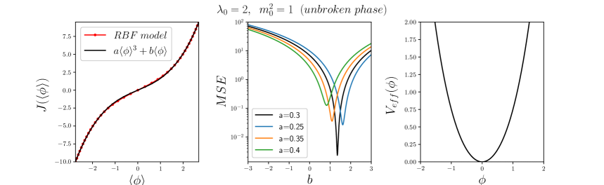
Figure 10: The obtained $J(\langle\phi\rangle)$ functional form calculated by the RBF model (red dots) for a set of $J$ background fields and the corresponding fit using Eq. 65 (black) for the unbroken phase. The middle plot shows the mean squared error for different $(a,b)$ combinations, while the right plot shows the obtained effective potential. The minimum of the mean squared error corresponds to $b>0$, which signals that the system is in the unbroken phase.

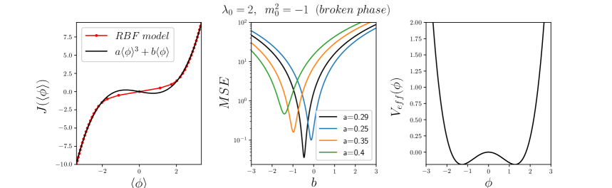
Figure 11: The obtained $J(\langle\phi\rangle)$ functional form calculated by the RBF model (red dots) for a set of $J$ background fields and the corresponding fit using Eq. 65 (black) for the broken phase. The middle plot shows the mean squared error for different $(a,b)$ combinations, while the right plot shows the obtained effective potential. The minimum of the mean squared error corresponds to $b<0$, which signals that the system is in the broken phase.

From Fig. 11, which corresponds to the broken phase, the previously described convexity problem is clearly visible through observing the discrete points coming from the numerical results (red dots). In this case the straight line between $\langle\phi\rangle\approx[-1.2,1.2]$ indicates that the phase is broken and there are two minima with a finite vacuum expectation value, which would correspond to a straight line between the two minima in $V_{eff}(\phi)$ in the case if we would naively use Eq. 61. By fitting the Ansatz for the effective potential from Eq. 65, we could overcome this problem as it is shown on the corresponding plot for $V_{eff}(\phi)$.

Considering all the above, the task that is to find the transition point that corresponds to the phase transition of the $\phi^{4}$ theory can be reformulated into finding the corresponding $m_{0}$ parameter for a fixed $\lambda_{0}$ coupling, where the best fit for the $J(\langle\phi\rangle)$ function (in the least square sense) has a transition from positive to negative $b$ values (unbroken $\rightarrow$ broken phase), thus, we are searching for the $b=0$ transition point. In Fig. 12, the RBF results for the phase transition points are shown together with previous Monte Carlo simulations on the lattice, taken from P11 and P12 . The comparison shows a very good match between the RBF expansion and the lattice result in a wide range of $(a^{2}\lambda_{0})$ coupling strengths.

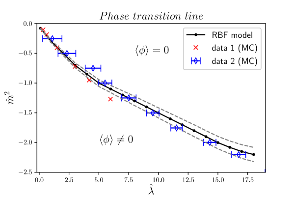
Figure 12: Phase transition line of the $\phi^{4}$ theory in 1+1 dimensions that is obtained from the RBF expansion (black) and compared to the results from lattice Monte Carlo simulations from P11 (red) and P12 (blue).

The uncertainty of the RBF results for each $(\hat{m}^{2},\hat{\lambda})$ pair has been estimated by calculating the standard deviation of the fitted $b$ parameter from the covariance matrices of the least squares estimate, then propagate the error to obtain the standard deviation of the $m_{0}$ parameter at fixed $\hat{\lambda}$, at the transition point, where $b=0$.

Considering our results it seems that the effective potential approach is sufficient to explain the behaviour of the phase transition line in the given coupling region. The next step in this direction would be to take the continuum limit and calculating the $f_{c}=\lambda_{R}/m_{R}^{2}$ critical coupling that characterizes the transition between the symmetric and broken phases.

5 Conclusions

In this paper a novel method is proposed to solve Euclidean path integrals for interacting systems in quantum field theories. The method is based on a radial basis function-type neural network expansion of the nonlinear interacting terms in the path integral, in which case the full discretized path integral can be expressed in a closed, analytically tractable form. The method makes it possible to calculate the generating functions, masses, vacuum expectation values, and other observables in a very fast and compact way that greatly exceeds the capabilities of other methods that aim to solve the nonperturbative regions of quantum field theories. The model has been tested for the lattice regularized interacting (real) scalar $\phi^{4}$ theory, where the mass renormalization and the phase transition from unbroken to broken phase have been studied. The renormalized masses have been calculated in the unbroken phase for a wide range of $\lambda_{0}$ coupling strengths, giving a monotonic increase with increasing coupling, which is expected from previous lattice simulations. To determine the phase transition line that separates the unbroken from the broken phase, the effective potential approach is used, where the vacuum expectation values of the averaged fields have been determined for a set of finite background field shifts, then, by examining the effective potential, the transition points were determined. The results have been compared to previous lattice calculations, giving a very good match between them.

The calculations are done for the lattice regularized $\phi^{4}$ theory, however, it is not limited to finite-sized lattices or finite lattice resolutions. In the first case the thermodynamic limit is straightforward to take, as in the case of any lattice technique, by doing the calculations in larger volumes and extrapolating the results for the observables to the infinite volume limit. On the other hand, taking the continuum limit is generally not a trivial task and requires a careful examination and scaling of the system at smaller and smaller resolutions. In contrast to lattice Monte Carlo methods, here, we do not have to consider such numerical problems like critical slowing down, which would otherwise make the simulations numerically very challenging. In general we could be able to make the calculations at any lattice resolution without any numerical complications, therefore, taking the continuum limit should not pose (at least) more numerical problems.

The generality of the RBF model makes it possible to estimate not just real but imaginary functional forms as well, in which case the path integral could be cast into a sum of generalized quadratic path integrals having real and imaginary parts. This representation could overcome the difficulties that arise in finite density calculations using Monte Carlo techniques, therefore, it could prove useful in describing finite density systems, where the Euclidean action consists of imaginary parts as well. In future works we aim to study such systems, e.g., in a non-Abelian gauge theory setting like quantum chromodynamics, where some other extensions would also be needed, e.g., including fermionic fields, taking care of gauge symmetries, etc.

The main advantage of the method at this stage is its speed and capability to study the nonperturbative aspects of interacting field theories. With some straightforward extensions, there is a possibility that in the future it could also be able to describe non-abelian gauge theories at finite densities, which is a necessary step in, e.g., describing the phase structure or vacuum properties of quantum chromodynamics and the strongly interacting matter.

References

- (1) F. Wilczek, Phys. Rev. Lett., 30, 1343–1346 (1973), arXiv:hep-th/0307346
- (2) M. Stevenson, Phys. Rev. D, 109, 014005 (2024), arXiv:2409.01228
- (3) S. Aoki et al., Eur. Phys. J. A, 49, 123 (2013), arXiv:1309.4200
- (4) A. Bazavov et al., Phys. Rev. D, 87, 054505 (2013), arXiv:1212.4768
- (5) Y. Aoki et al., Nature, 443, 675–678 (2006), arXiv:hep-lat/0611014
- (6) A. Bazavov et al., Phys. Rev. D, 98, 074512 (2018), arXiv:1712.09262
- (7) T. Iritani et al., Phys. Rev. D, 99, 014514 (2019), arXiv:1805.04150
- (8) P. Lepage, Phys. Rev. D, 59, 074502 (1999), arXiv:hep-lat/9809157
- (9) K. Nagata, Prog. Part. Nucl. Phys., 123, 103991 (2022), arXiv:2108.12423
- (10) Z. Hanada et al., Phys. Rev. D, 86, 074510 (2012), arXiv:1207.1915
- (11) AA. Alexandru et al., Rev. Mod. Phys., 94, 015006 (2022), arXiv:2106.05934
- (12) V. A. Goy et al., Prog. Theor. Exp. Phys., 2017(3), 031D01 (2017)
- (13) Y. LeCun, Y. Bengio, and G. Hinton, Nature, 521, 436–444 (2015)
- (14) U. Schmidhuber, Neural Networks, 61, 85–117 (2015)
- (15) Y. Che, C. Gneiting, F. Nori, Phys. Rev. B. 105, 21 (2022). http://dx.doi.org/10.1103/PhysRevB.105.214205
- (16) G. Balassa, ’On the solution of Euclidean path integrals with neural networks’ (2025), arXiv:2509.16953 [hep-ph]
- (17) J. Zinn-Justin, Quantum Field Theory and Critical Phenomena, Int. Ser. Monogr. Phys., Oxford University Press, 4th ed. (2002)
- (18) M. J. D. Powell, Comput. Appl. Math., 123, 145 (2000)
- (19) R. P. Feynman, Rev. Mod. Phys., 20, 367 (1948)
- (20) U. Mosel, Path Integrals in Field Theory: An Introduction, Springer-Verlag, Berlin Heidelberg, Advanced Texts in Physics, (2004), ISBN: 978-3-540-21056-9
- (21) N. V. Quan, M. T. Long, Electrical Engineering, 111, 1123 (2025)
- (22) Y. Liao, S.-C. Fang, and H. L. Chen, IEEE/ACM Trans. Comput. Biol. Bioinform., 8, 187 (2011)
- (23) G. Balassa, Prog. Theor. Exp. Phys., 2023, 113A01 (2023)
- (24) M. H. Hassoun and M. A. Ali, IEEE Trans. Neural Netw., 10, 524 (1999)
- (25) T. Schaefer and E. V. Shuryak, Rev. Mod. Phys., 70, 323 (1998)
- (26) M. E. Peskin and D. V. Schroeder, An Introduction to Quantum Field Theory, Addison-Wesley, Reading, MA, (1995), ISBN: 978-0201503975
- (27) J. M. Pawlowski, I.-O. Stamatescu, F. P. G. Ziegler, Phys. Rev. D, 96, 114505 (2017)
- (28) C. Itzykson, J.-B. Zuber, Quantum Field Theory, McGraw-Hill, New York, (1980), ISBN: 978-0070320710
- (29) M. Srednicki, Quantum Field Theory, Cambridge University Press, 2007, ISBN: 978-0521864497
- (30) S.-K. Jian, E. Barnes, S. D. Sarma, Phys. Rev. Res., 2, 023310 (2020),
- (31) J. R. Klauder, C. B. Lang, P. Salomonson, B.-S. Skagerstam, Z. Phys. C, 26, 149 (1984)
- (32) W. D. McComb, Renormalization Methods: A Guide for Beginners, Oxford University Press, 1st Edition (2008), ISBN: 9780199236527
- (33) A. K. De, A. Harindranath, J. Maiti, T. Sinha, Phys. Rev. D, 72, 094503 (2005)
- (34) F. K. Diakonos, Y. F. Contoyiannis, S. M. Potirakis, Prog. Theor. Exp. Phys., 2021, 043A01 (2021)
- (35) N. Goldenfeld, Lectures on Phase Transitions and the Renormalization Group, CRC Press (1992)
- (36) S. Akiyama, Y. Kuramashi, Y. Yoshimura, Phys. Rev. D, 104, 034507 (2021)
- (37) T. Inagaki, S. Nojiri, S. D. Odintsov, JCAP, 0506, 010 (2005)
- (38) J. Alexandre, Phys. Rev. D, 86, 025028 (2012)
- (39) R. W. Haymaker, J. Perez-Mercader, Phys. Rev. D, 27, 1948 (1983)
- (40) K. Tabata, I. Umemura, Prog. Theor. Phys., 74, 1360 (1985)
- (41) D. J. E. Callaway, D. J. Maloof, Phys. Rev. D, 27, 406 (1983)
- (42) N. Straumann, Cosmological Phase Transitions, arXiv:astro-ph/0409042 (2004)
- (43) Lewis H. Ryder, Quantum Field Theory, Cambridge University Press, Cambridge, 1985. ISBN: 9780521237642
- (44) W. Loinaz, R. S. Willey, Phys. Rev. D, 58, 076003 (1998)
- (45) A. Ardekani, A. G. Williams, Austral. J. Phys. 52, 929 (1999).
- (46) K. Binder, Z. Phys. B, 43, 119 (1981).
- (47) A. Milchev, D. W. Heermann, K. Binder, J. Stat. Phys., 44, 749 (1986).