Deep Learning-Driven Peptide Classification in Biological Nanopores

Abstract

A device capable of performing real time classification of proteins in a clinical setting would allow for inexpensive and rapid disease diagnosis. One such candidate for this technology are nanopore devices. These devices work by measuring a current signal that arises when a protein or peptide enters a nanometer-length-scale pore. Should this current be uniquely related to the structure of the peptide and its interactions with the pore, the signals can be used to perform identification. While such a method would allow for real time identification of peptides and proteins in a clinical setting, to date, the complexities of these signals limit their accuracy. In this work, we tackle the issue of classification by converting the current signals into scaleogram images via wavelet transforms, capturing amplitude, frequency, and time information in a modality well-suited to machine learning algorithms. When tested on 42 peptides, our method achieved a classification accuracy of  $81\,\%$, setting a new state-of-the-art in the field and taking a step toward practical peptide/protein diagnostics at the point of care. In addition, we demonstrate model transfer techniques that will be critical when deploying these models into real hardware, paving the way to a new method for real-time disease diagnosis.

These authors contributed equally to this work. These authors contributed equally to this work.

1 Introduction

Recent developments in cancer research have indicated that specific chains of amino acids within a biological sample can serve as early indicators for certain cancers, potentially years before initial diagnosis ¹. This discovery opens a promising avenue for early cancer detection by the recognition of these amino acid chains, typically proteins or their smaller counterparts, peptides, within biological samples. Indicators can manifest as elevated levels of common proteins or the presence of post-translational modifications (PTMs), changes to a protein or peptide after biosynthesis. In their 2023 paper, Barker et al. ² highlight current research stating that as of 2022, 3,224 peptides along with 1,742 proteins have been validated by the Clinical Proteomic Tumor Analysis Consortium (CPTAC) ³ for use in the development of reproducible assays for cancer biomarkers ^{4, 5}. For this reason, fast, low-cost, accurate methods for identifying large numbers of proteins, peptides, and PTMs with single-molecule precision would be breakthroughs. Traditional methods for protein identification include mass spectrometry ⁶ on samples containing thousands of proteins and peptides or on individual proteins separated via gel electrophoresis ⁷. In both cases, the process is expensive, time-consuming and importantly, requires processing in a laboratory separated from clinicians, thus prohibiting real time, on-premises diagnosis. Nanopore-based classification devices have significant potential to remove these hurdles from the field of identification process ⁸, ⁹. Nanopores are nanometer scale ($1e^{-9}m$) channels in a membrane into which an analyte, be it DNA, a protein, or a peptide, can be driven. These nanopores can be solid-state ¹⁰, such as holes in graphene sheets, or biological ¹¹, built out of pore-forming porin molecules such as Aerolysin. When being used for sequencing or classification, a voltage is applied across the nanopore channel, driving charge carriers in the surrounding fluid through the pore, creating a measurable current. As an analyte enters the pore, the charge carriers will be impeded, reducing the measured current and producing what is referred to as a blocking, or blockade current. Due to the simplicity of this process, devices built for nanopore classification are small and can be operated with very little pre-processing, making them a promising candidate for clinical applications.

Nanopore technology first emerged as a means for sequencing DNA, whereby a pore is reconstituted on a membrane, and a motor enzyme is placed over the pore that can then act as a ratchet to pass sets of DNA bases into the pore at a time ¹². The bases presence inside the pore induces a blockade current that can then be used to identify them ¹³, ¹⁴, ¹⁵, ¹⁶, ¹⁷. As this approach proved useful for DNA sequencing, a natural progression would be to apply them to the more complex case of proteins, starting with peptides. However, this extension presents a series of challenges. The first problem is the absence of a ratcheting mechanism that could pass a peptide one amino acid at a time into the pore for measurement, although research is ongoing to solve this problem ¹⁸. In the approaches studied here, the entire peptide is trapped in the pore for a varying period of time before leaving it. The second challenge arises from the complexity of the proteins and peptides. Unlike DNA, which has four base pairs, peptides are constructed from 20 different kinds of amino acids, which are themselves complex molecules. These factors result in non-trivial blockade currents, impacted by the geometry of the peptide in the pore, interactions with the pore walls, and charge carriers in the solution. While limited sequencing success has been achieved ¹⁹, ²⁰, ²¹, typically, and as will be the case here, the focus is on classifying individual peptides and proteins within a mixed solution in real time, as one would require in a clinical setting.

Prior work has approached this problem from a variety of different angles. Afshar Bakshloo et al. ²² and Ouldali et al. ²³ have shown that the mean blockade current, primarily related to the volume of the shape formed by the peptide in the pore, can be used to identify several samples. Zhang et al. ²⁴ and Cao et al. ²⁵ demonstrated that specific machine learning methods, such as Random Forest or nearest-neighbor algorithms, can be used to identify specific residues on a peptide chain when passed individually into the pore, with results shown using small dense neural networks ²⁶. In the direction of peptide classification on a large number of classes, recent work using statistical moments of blockade current-formed distributions was shown to classify up to 42 such peptides with approximately 70 % precision ²⁷, setting the standard to beat in the field. This work introduces a new approach to peptide classification in nanopore experiments by leveraging the image classification capabilities of deep neural networks. Specifically, we convert blockade currents for single events into so-called scaleogram images via a wavelet transformation ²⁸ capturing time, frequency, and amplitude information. Deep vision models, including a ResNet-18 ²⁹, ResNext101 ³⁰, and a Vision Transformer (ViT) ³¹ are then trained on the classification task, achieving up to 81.7 % overall classification accuracy on 42 peptides. The results outlined here represent not only the state-of-the-art in peptide classification using nanopore experiments, but also a practical means to accelerate peptide and protein classification, both essential steps towards clinical applications of this potentially groundbreaking technology.

2 Results

Data Collection and Processing

Initial data was generated by nanopore experiments carried out at the University of Freiburg ^{32, 33}, details of which can be found in Section 4. Figure 1 illustrates the physical process, reproduced in simulation, by which a small peptide in a bath of ions enters a pore reconstituted in a membrane.

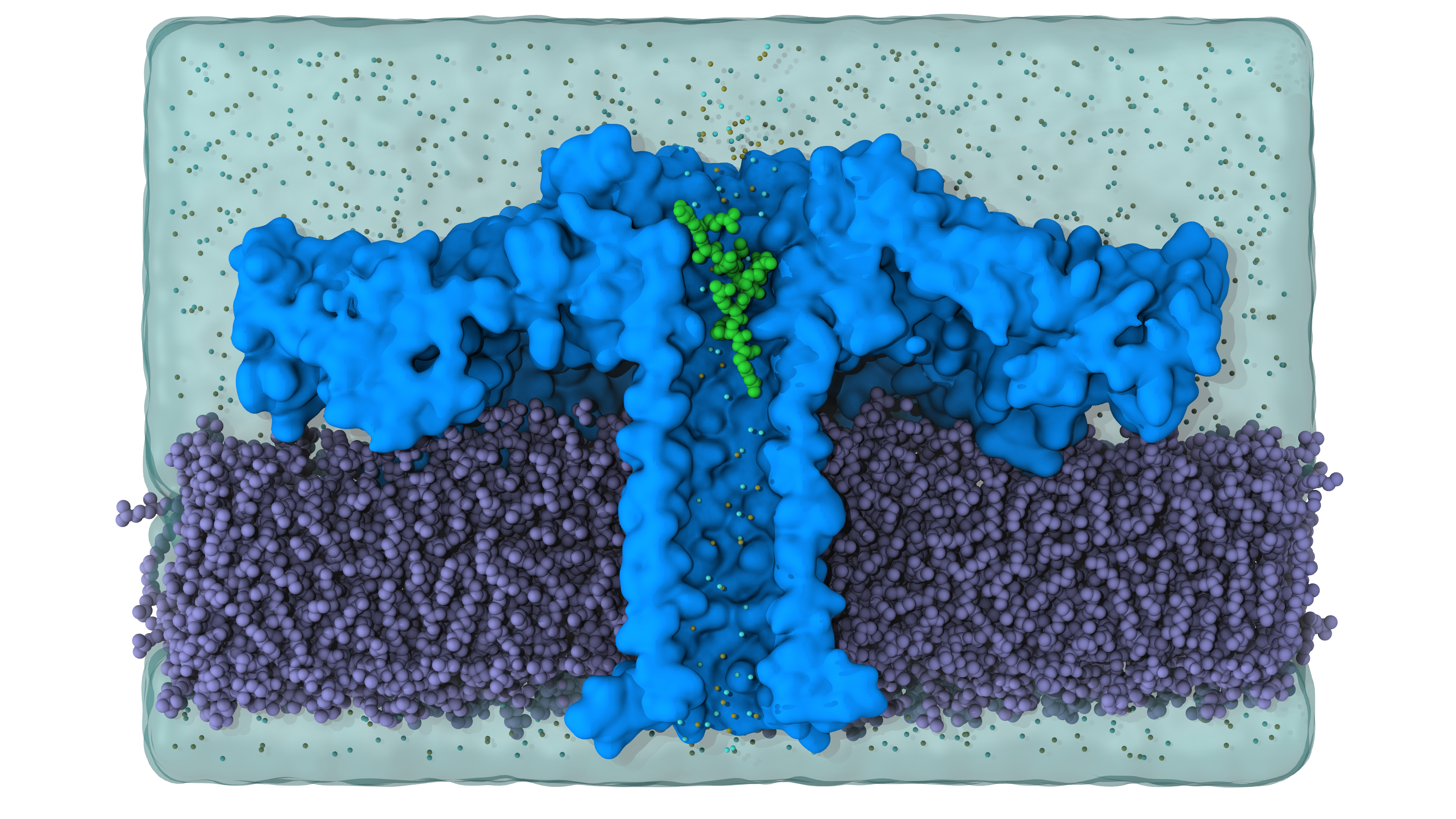
Figure 1: Rendering of the nanopore embedded in a DPhPC lipid bilayer with a peptide (green) at the pore’s entrance. The surrounding fluid also contains charged ions, represented as free spheres in the fluid.

Experiments such as these generate large current sequences from which individual events must be extracted and labeled. In Figures 2 a) and b), the raw data extracted from the experiments, together with an event extracted, are displayed.

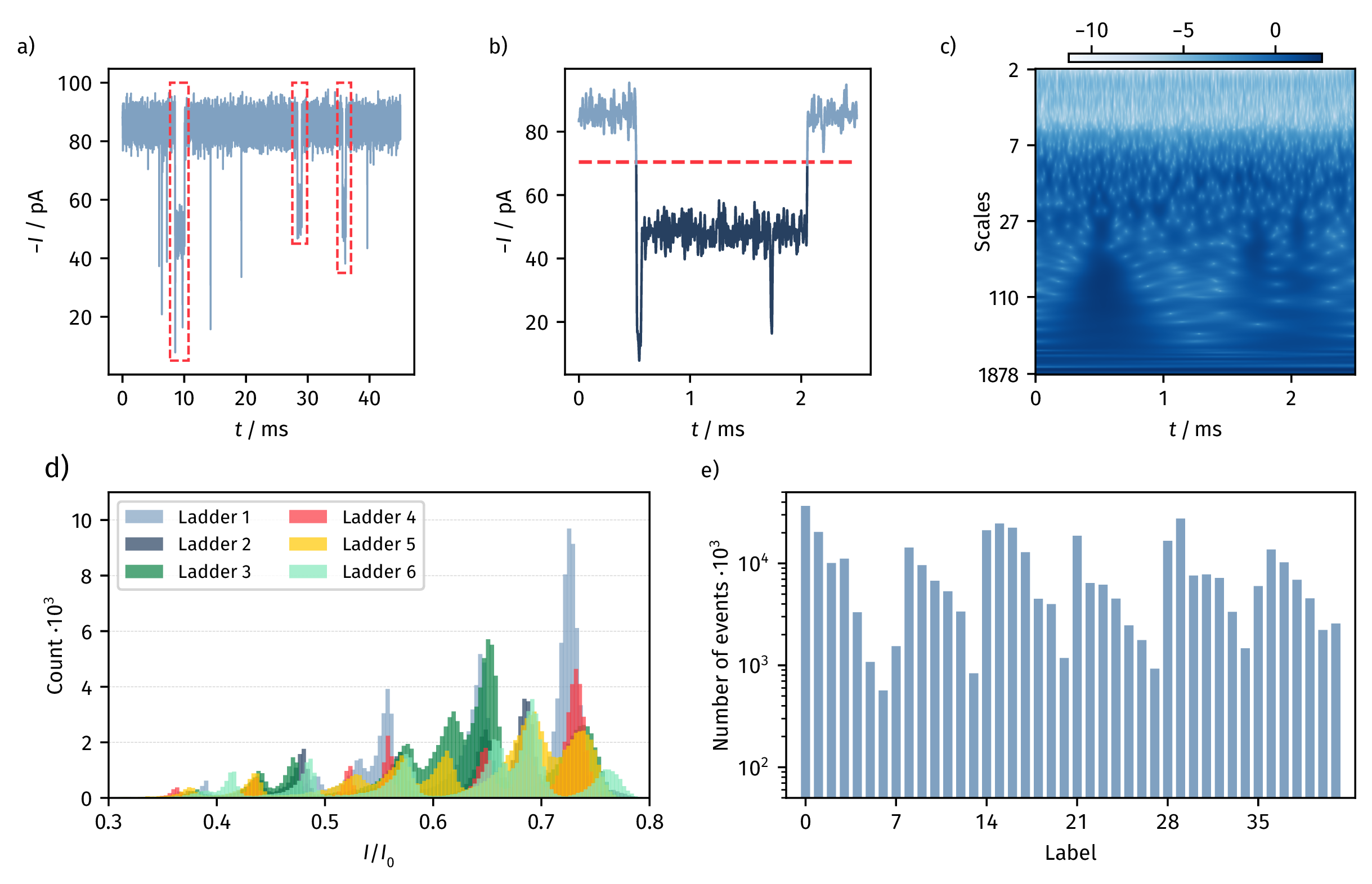
Figure 2: Example data pipeline from experimental readout to wavelet transforms. a) Data is read from an experiment, resulting in a range of events corresponding to peptides entering the pore. b) Events are detected using a standard, three-sigma algorithm. c) A wavelet transform is applied to individual events, resulting in a scaleogram. d) Histograms of the individual peptide ladder experiments, overlapped in order to highlight the need for advanced classification algorithms, as simple mean-current analysis will not suffice to identify single peptides from a mixture of these peptide ladders. e) Distribution of extracted, labeled events, split into the training, validation and test sets chosen such that the label imbalance was preserved.

The event extraction process is elaborated in Section 4. These extracted events can be used to construct histograms of the relative blockade current of all the peptides available for classification, as outlined in Figure 2 d), where 42 peaks correspond to the 42 peptides in the solutions. The fact that these histograms overlap to such a degree represents the limitation of blockade current averages to distinguish between many peptide classes. Finally, in Figure 2 e), a histogram of the data quantity per class is outlined to highlight the imbalance of samples between the classes used in training. This data is further split into train, test, and validation sets during the training process, reducing the amount of data that can be learned.

Wavelet Transformations and Scaleogram Construction

Once the data is extracted and labeled, each blockade current (Figure 2 b) as an example) is converted into a complex-valued scaleogram image via continuous wavelet transform using the ssqueezepy Python package ³⁴, the result is shown in Figure 2 c), by taking the absolute value of the transform for each pixel. Detailed information on the wavelet transformation can be found in Section 4. The scaleogram contains all of the time and frequency information from the current signal, represented as an image, a format more suitable for machine learning. For training, the absolute value of the continuous wavelet transform is used, and an element-wise logarithm of the values is applied before resizing in order to improve the numeric stability of the training.

Model Training and Classification Performance

In order to assess the functionality of image representations for peptide classification, three neural network architectures were chosen due to their ubiquity and state-of-the-art performance on vision tasks. These networks included a ResNet18 ²⁹, a ResNeXt101 ³⁰, and a Vision Transformer ³⁵. Additional details about the architectures and how they were trained can be found in Section 4. Table 1 outlines the final macro, micro, and top-10 accuracies produced by each model and a comparison to prior work ²⁷.

Table 1: Test performance of the classifier models used in this investigation, along with a comparison to prior work ²⁷.

Averaging	ResNet18	ResNeXt101	Vision Transformer	catch22 27
Macro	81.7 %	79.0 %	80.9 %	73.6 %
Micro	81.5 %	79.1 %	80.4 %	73.6 %
Top-10	84.9 %	82.5 %	84.2 %	75.8 %

Here, the macro accuracy is defined as the average of all per-class accuracies, whereas the micro accuracy simply denotes the ratio of correct predictions to the total number of events in the test dataset. Finally, the top-10 accuracy denotes the average accuracy of the ten classes with the most samples in the dataset. The models trained on the scaleograms outperform our previous approach of using the catch22 feature set by over 5 % percentage points in all shown metrics. The ResNet18 model achieves the best overall performance, reaching a macro accuracy of over 81 %. Although this suggests that the ResNet18 architecture is best suited for this task, we believe that this result is limited by the amount of training data. This is supported by the fact that the top-10 accuracies of all models are higher than the respective macro accuracies, indicating a better performance with more data. Furthermore, the ResNeXt101 model performs worse than the ResNet18 model, even though the larger model should, in principle, outperform their smaller counterparts given sufficient data ³⁶. Due to experimental constraints on data generation, the networks were only trained on $260,000$ images, far below the standard in larger vision models such as the ImageNet benchmark ³⁷. The results therefore suggest that the larger ResNeXt101 has not reached its limit in performance, and the models will continue to improve with more data.

To understand the misclassifications by the models, we plot the confusion matrices computed over the test dataset, as shown in the upper portion of Figure 3. These 42 by 42 matrices are constructed by populating their elements with the test samples, where the row corresponds to the sample’s label, and the column is given by the model’s prediction. For a complete list of which peptide corresponds to which label, see Table 1 in the Supplementary Information. A larger number on the diagonal therefore corresponds to a better performance of the model, whereas off-diagonal elements in the confusion matrices highlight classes that are confused with others. In the confusion matrices, a periodic pattern in the off-diagonals can be observed. These elements correspond to misclassifications of peptides with equal-length peptides from other ladders, whose mean blockade current histograms also show partial or complete overlap. Whether these misclassifications stem from the numerical transformation of these similar currents into scaleograms or reflect intrinsic similarities in peptide dynamics within the pore, cannot be conclusively determined from our results and is a subject for future investigation.

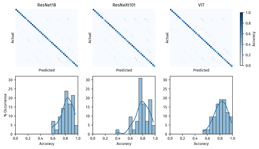
Figure 3: Confusion matrices and accuracy distribution for the ResNet18, ResNeXt101 and Vision transformer architectures assessed throughout this work. Here, the accuracy denotes the per-class accuracy, where row-wise normalization was performed.

Further insights on the subtle differences between the model results is gained by looking at the distribution of macro accuracies of the models, shown in the lower portion of Figure 3. The overall classification performance varies notably across models. ResNet18 demonstrates the best overall performance, with a narrower distribution of class accuracies that is shifted closer to 1. In contrast, the ResNeXt101 shows a broader distribution, reflecting a greater variability in the class-wise accuracy. In terms of minimal class accuracy, differences between models are also evident: for the particularly challenging class L2AA4, the ResNeXt101 model achieves the lowest accuracy at $38.5\,\%$. This improves to $53.3\,\%$ with the Vision Transformer, and reaches $60.2\,\%$ with the ResNet18 model. However, the ResNet18’s performance is likely related to the limited size of the training dataset, and we expect the more complex models to outperform it with more data.

Importance analysis

The scaleogram representation allows for a frequency-resolved interpretation of relevant dynamics in the signals as predicted by the trained models. To realize this, a DeepliftSHAP analysis was performed using the captum framework ³⁸ and the best-performing ResNet18 architecture. Further implementation details can be found in Section 4.

Figure 4 shows a visualization of the important regions for six randomly chosen samples of the test dataset. All of the images exhibit a high importance in the lower corners of the scaleogram, reflecting rise- and fall-events of the blockade current, capturing information about the magnitude of the current blockade. More surprisingly, however, some signals show a high importance score in the upper portion of the scaleogram. This indicates that the model can recognize certain aspects in the high-frequency portions of the signal that are dominated by noise.

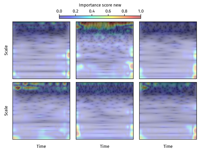
Figure 4: Visualization of important regions in the scaleogram for randomly chosen events from the test dataset. The scaleogram is visualized in the background, with important regions shown in red. The important regions are broadened for better visualization.

Model Transfer

A critical aspect for the use of the classification algorithm in diagnostics is the ability to deploy the trained models locally. Allowing for local deployment will improve data security and provide a means for offline functionality, essential in many point-of-care applications ³⁹. However, as these models become larger and handle more classes, the problem of deploying them into a device will be challenging to solve. To this end, we explore the performance of the three introduced models after undergoing a model-transfer pipeline. In realistic model transfer cases, this pipeline consists first of methods to reduce the size and complexity of the networks via weight pruning ⁴⁰, ⁴¹, ⁴² and quantization ⁴³, ⁴⁴. Weight pruning involves removing network parameters based on their magnitude and is often characterized by a removal fraction, the percentage of parameters that were removed. Quantization reduces the precision of parameter values by mapping them to a smaller set of discrete levels in a lower-bit representation. For pruning, both structured and unstructured weight pruning were studied; however, only the global unstructured pruning produced usable results. Details on the implementation can be found in Section 4. To measure the effect of pruning, the micro and macro accuracy scores are computed to demonstrate how the models’ performance deteriorates after pruning. Figure 5 outlines the results of this investigation.

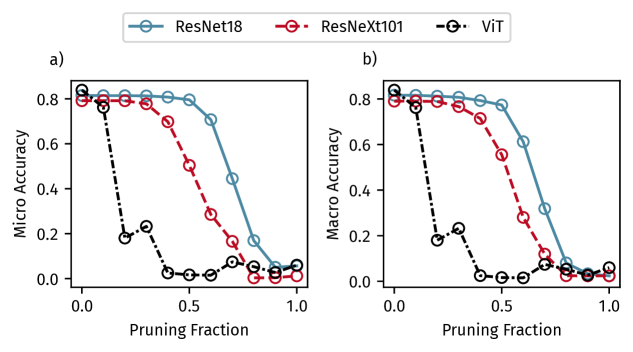
Figure 5: Micro accuracy (a) and Macro accuracy (b) of the models as a function of the pruning fraction.

Micro and macro accuracy reveal identical trends, corroborating degradation to be class-independent. The ResNet18 model appears to be the most resilient to pruning, retaining its accuracy until up to $50\,\%$ of its weights have been pruned. The ResNeXt101 shows similar resilience, whereas the ViT architecture is far more sensitive. While these results are promising, it should be noted that in well-trained models, pruning up to $90\,\%$ can be achieved without significant degradation of model performance ⁴². This result is merely a demonstration that the models can be improved and optimized for hardware deployment once trained on sufficient data, particularly in the case of the ViT models, where many alternative pruning and model reduction approaches are being developed ⁴⁵. However, it also shows a limitation of the current models in that they are likely not sufficiently well trained to have constructed stable latent space representations and therefore, are highly sensitive to changes in their structure. Remedies to this problem can include adding dropout-style training into the optimization procedure, but would likely also be aided by sufficient training data.

For quantization, we used Post Training Static Quantization for the ResNet18 and ResNeXt101 models, and Dynamic Quantization for the Vision Transformer, using PyTorch’s Quantization framework ⁴⁶. The ResNet18 and ResNeXt101 models were calibrated on the validation dataset, and all quantized models were benchmarked on the test dataset. The results are shown in Table 2. Among all three models, the ResNet18 achieves the most effective compression with a minimal drop in macro accuracy of $0.6$ percentage points. The ResNeXt101, while also achieving a comparable reduction in size, suffers from a significant reduction in performance. In contrast, the Vision Transformer shows a more modest decrease in size paired by a moderate performance loss. These differences in performance degradation for both the model pruning and quantization can mainly be attributed to the differences in architecture and parameter redundancy due to the size of the models. With more data, as well as more sophisticated pruning and quantization methods, we are confident that the ResNeXt101 model and the Vision Transformer can outperform the ResNet18 architecture.

Table 2: Results of the model quantization. FP32 denotes the single-precision floating point format, whereas I8 denotes the signed 8-bit integer format. The bold numbers in the model size column indicate the compression factors of the quantised models.

Model	# Parameters $\cdot 10^{6}$	Precision	Size in MB	Accuracy
				Macro	Micro
ResNet18	$11.2$	FP32	$44.8$	$81.7\,\%$	$81.5\,\%$
		I8	$11.3$ ($\sim\mathbf{3.96x}$)	$80.9\,\%$	$80.3\,\%$
ResNeXt101	$81.5$	FP32	327	$79.0\,\%$	$79.1\,\%$
		I8	$83.5$ ($\sim\mathbf{3.92x}$)	$70.3\,\%$	$68.0\,\%$
ViT	$9.63$	FP32	$38.58$	$80.9\,\%$	$80.4\,\%$
		I8	$19.5$ ($\sim\mathbf{1.97x}$)	$78.5\,\%$	$77.8\,\%$

3 Discussion

In this study, we have shown that image-based machine learning algorithms, including convolutional and transformer-based, achieve up to $81.7\,\%$ total accuracy in nanopore-based peptide signal data on 42 unique classes, many of which have similar geometry and therefore subtle differences in their current signals. These images are constructed via wavelet transformations that convert a one-dimensional time series of electrical current into an image capturing time, frequency, and amplitude.

During the study, we tested several architectures, namely ResNet-18, a larger ResNeXt-101, and finally, a vision transformer, with the ResNet-18 producing the best results after training. Given the assumption that larger models are more capable of learning features and thus should produce better results, we expect that this trend is largely due to the limitations on data quantity and that the other, larger architectures would eventually outperform the ResNet-18. In any case, the performance reached by ResNet-18 outperformed the prior state-of-the-art approach ²⁷. While these results were adequate, they leave significant room for enhancement. With only 42 peptide classes, this work addresses a small percentage of the number currently accepted for use in disease diagnoses, leaving the door open for improvement. In the field of image classification, large machine-learning architectures can achieve accuracies of 91 % on datasets with 1000 classes ⁴⁷ and 77.6 % on datasets with 21,000 classes ⁴⁸. Therefore, it is our opinion that with increased training data and algorithmic improvements that the introduced approach to peptide classification can be extended to a clinically significant number of classes.

In order to further analyze the performance of the models, we computed importance scores for the regions of the scaleogram images using the DeepliftSHAP framework. This allows better understanding of how specific features in the image impact the model’s predictions, thus highlighting important regions. We found, interestingly, that the noise-dominated high-frequency regions of the image were of particular importance to the predictions. Importance in these regions suggests that there are relevant processes taking place on short time-scales at this resolution, thus motivating the use of either high resolution measurements at high bandwidth or computational studies at time-scales that are able to extract signal components from noise affected data. Additional importance was attributed to the entry and exit in the pore, as indicated by bright regions at the left and right edges of the image. Beyond highlighting possibly important time-scales for relevant processes, these importance scores also allow speculation on how to isolate feature vectors ideally that may be used to identify specific peptides more rapidly and formulate a database of peptide fingerprints in the future.

Finally, to demonstrate an important step in the developed of offline, possible embedded devices, we performed model transfer studies. Whether used in point-of-care settings or to comply with data privacy regulations, nanopore-based diagnostics may require offline-capable and easily portable devices during deployment. Such devices would necessitate the compression of the models as much as possible to improve power consumption and latency. Our results demonstrated that as much as 50 % of the model weights could be removed without a drop in accuracy, with a proportional reduction in model size. Further, quantization achieved a near four times reduction in the size of the models with little to no degradation in the most robust architecture.

Additional research could explore the use of quantization ⁴⁹- and pruning-aware training (via dropout) to incorporate these features into the training process. Additionally, we perform no speed or scaling-based experiments here to identify bottlenecks and possible improvements in the full pipeline. Such an investigation could make use of additional model transfer techniques, including layer fusion and computational graph optimization via the ONNX or TensorRT libraries.

4 Methods

Peptide Ladder

This work applies classification models to 42 peptides in the form of peptide ladders ³². Figure 6 reveals the structure of the six peptide ladders used in the study.

Figure 6: Visualization of the peptide ladders used in the investigation. For each ladder, amino acids can be cleaved individually starting from the N-terminus up to the three Arginine (R) bases on the C-terminus. Thus, for each complete ladder, 6 smaller sub-ladders can be constructed, providing a total of 7 samples. Given the 6 available ladders, this results in 42 total peptides for consideration.

The far left side shows the N-terminus indicated by H, and the far right shows the C-terminus denoted as OH. Letters S, R, A, K, and Y correspond to the amino acids Serine, Arginine, Alanine, Lysine, and Tyrosine. The shaded blocks on the C terminus are fixed in all studies, whereas light blocks can be removed in an experiment. Each of the six peptide ladders consists of seven possible blocks, ranging from decapeptides to tetrapeptides, resulting in a total of 42 distinct peptide classes.

Event Detection and Labeling

During nanopore experiments, a time series of current measurements is captured, within which many events will occur, as shown in Figure 2 a). Before these events can be classified, they are isolated from the long current readout into single events and stored as single events. As a pre-processing step, a wavelet threshold filter using the bior1.5 wavelet and a hard threshold of $0.5$ was applied to the raw data. A statistical threshold detection approach ³³, ²⁵ is then performed, wherein deviations from the Gaussian-like distribution of the open-pore current are used to detect the onset of an event. During event detection, the signal is processed in series, computing a windowed average over the pore current to allow for changes in the open-pore values. If the current falls below three standard deviations, $\sigma$, from the open-pore value, it is considered to be the start of an event. If an event is found to have a mean current below a second threshold of $4\sigma$, it is ignored as an outlier, in line with the first method introduced in Piguet et al. ³³. Further reduction of spurious events was achieved by only allowing events with a dwell time greater than $80\text{\,}\mathrm{\SIUnitSymbolMicro s}$, attributing for the instrumentation’s temporal resolution. Finally, all detected events were normalized by the mean of the surrounding open pore current.

Histograms of the current values from single ladder experiments can then be analyzed and labeled. Labeling is performed by first fitting the peaks of the histograms with Voigt profiles ⁵⁰. Peptide-specific events were then identified if they fell within each profile’s full-width-half-maximum (FWHM). This discrimination of events for labeling poses a potential source for errors, as neighboring histograms overlap and may, therefore, fall within the FWHM of their neighbor, thus ending up falsely labeled. In practice, each ladder, L1-6, was studied individually. Therefore, labeling is done using the normalized blockade current histogram for all measurements of a specific ladder, thus, there are no labeling errors between peptides with the same number of amino acids, i.e., those with the most significant overlaps. However, as with most ML classification tasks on large data sets, we expect a small amount of labeling error, likely due to the overlap in current histograms for sub-ladders of a single ladder, something that can seen in Figure 2 d). Measuring the amount of false labeling and the impact on the models is a subject for future investigation.

Scaleogram Image Construction

A scaleogram is an image formed by performing a wavelet transformation on raw time-series data ⁵¹ by

$$W(a,b)=\frac{1}{\sqrt{|a|}}\int_{-\infty}^{\infty}x(t)\,\psi^{*}\left(\frac{t-b}{a}\right)dt$$ (1)

with $\psi(x)$ the mother wavelet, as shown in Figure 2 c) with the time parameter (b) on the $x$-axis and frequency, $a$ on the $y$-axis. Such an operation produces an image where each pixel corresponds to a single $(a,b)$ coordinate and color corresponding to the solution of Equation 1. Thus, after a wavelet transform, all of an event’s time, frequency, and amplitude information is converted into image data, for which machine-learning approaches are particularly well suited. In the investigations, the ssqueezepy Python library ³⁴ was used to perform the wavelet transforms using the hhhat wavelet with parameter $\mu=5$. Although this wavelet has led to optimal results, more training data and further optimization of the wavelet may enhance classification performance, and optimizing this wavelet is subject to future research. Images were then resized to a width and height of 224 pixels through a bilinear interpolation.

Classifier Models

This study explores the use of images for peptide classification and requires neural network architectures capable of processing these images. The training data consists of approximately $350,000$ images containing 42 classes to be classified. In this study, the ResNet18 ²⁹, ResNeXt101 ³⁰, and a Vision Transformer ³¹, the parametrization of which is presented in Table 3, were chosen due to their wide acceptance in the community.

Table 3: Network architectures used in the study.

Model Name	Layer Type	Number of Parameters
ResNet18	Convolutional	11,194,922
ResNeXt101-64x4d	Convolutional	81,489,194
Vision Transformer	Transformer	9,634,218

All models were implemented within the PyTorch framework ⁴⁶ and trained on two NVIDIA L4 GPUs. PyTorch Lightning was used for the multi-device training routine ⁵². For all models, input images were normalized based on the mean and standard deviation of all pixel values in the training dataset to avoid potential data leakage. During training, the inputs were subject to image augmentations, including random erasure ⁵³, horizontal and vertical flips and random resize-cropping. Image augmentations of this kind have been shown to improve model generalization and have the effect of artificially expanding the dataset ⁵⁴. Furthermore, all models were trained to minimize a categorical cross-entropy loss function as implemented in PyTorch. Both the ResNet18 and ResNeXt101 architectures were initialized using pre-trained weights from models trained on the ImageNet dataset ³⁷ as this has been shown to improve classification performance ⁵⁵. The ResNet18 and ResNeXt101 models were trained using stochastic gradient descent with a momentum of $0.9$ ⁵⁶ and a weight decay of $10^{-4}$, and a multi-step learning rate scheduler was deployed. Due to the size of the dataset and the models, the ResNeXt-101 and ResNet-18 were trained using 100 mini-batches of 50 images, resulting in an effective batch size of $5000$ images. Finally, Stochastic Weight Averaging ⁵⁷ was employed as implemented in the PyTorch Lightning package, as it has been shown to improve performance after initial training ⁵⁸. Overall, the models were allowed to train for $1000$ epochs, although model training was stopped early when no improvement was expected.

The Vision Transformer utilized in this work consists of twelve transformer blocks, each with four attention heads. To construct the input to the transformer, 14x14 pixel blocks were flattened and passed through a single dense network layer, projecting them into a 256-dimensional representation. An additional learnable positional embedding was applied to correlate the patches in the transformer.

Training the Vision Transformer was performed in two steps, in line with the work from which the architecture is taken ⁵⁹. The first step involves unlabeled pre-training, as outlined in Figure 7.

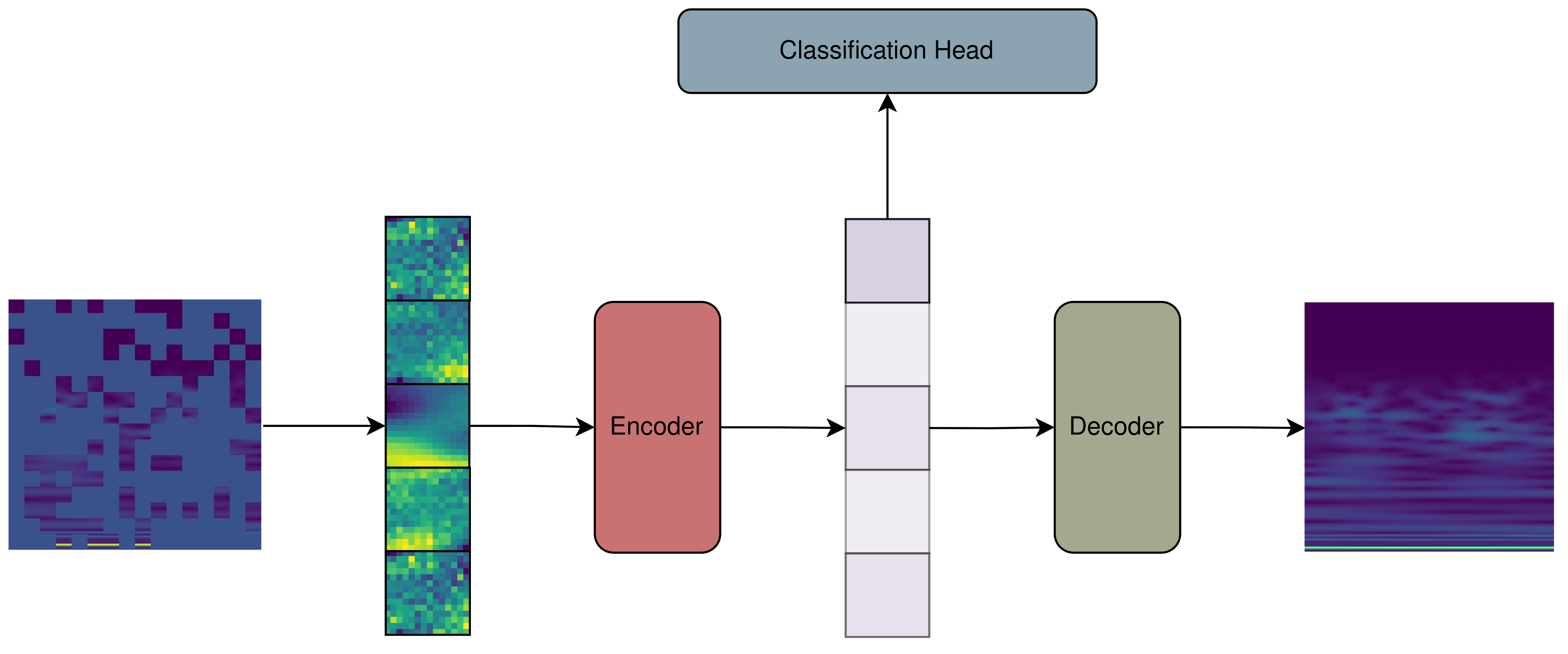
Figure 7: The encoder-decoder architecture used in pre-training the Vision Transformer. Initially, a wavelet image is divided into input patches. During pre-training, $70\,\%$ of the patches are masked, while the remaining ones are passed into the encoder. The encoder generates a latent space representation, which is then concatenated with the masked patches and passed through the decoder, aiming to reconstruct the original image. After pre-training, the classification head uses the pre-trained latent space representation for the classification task.

During this phase, $70\,\%$ of each image is masked using a learnable mask token, with the remaining visible patches passed into the transformer encoder. The output of this pass is then concatenated with the mask tokens in the original order and passed through a decoder block of the same architecture as the transformer encoder. This decoder block produces a reconstructed image that is then compared to the original, unmasked image. The model was trained to reconstruct the full image accurately from the sparse chunks it receives correctly. Training took place with an effective batch size of 1600 images split into eight minibatches of 200. The learning rate was set first by a linear warm-up to an ADAM optimizer, followed by a cosine decay ⁶⁰ with a max value of $1\cdot 10^{-4}$ throughout the rest of the training. This pre-training has the effect of tuning the latent space representation of the encoder transformer, which will later be used for classification, such that it can completely reconstruct its input, an approach shown on many occasions to improve classification performance ⁶¹, ⁶². Further, as pre-training does not require labeled data, it can be exposed to more peptide events than the classification training.

Once pre-training was completed, the classification head, a one-layer dense network with GELU activation function ⁶³ of architecture $\left(\mathcal{D}^{128}\cdot\text{GELU}\cdot\mathcal{D}^{42}\right)$, was trained on the classification task, taking the latent space generated by the encoder as input. As fine-tuning the encoder’s latent space representation during the classification task further improves performance, both the classification head and the transformer encoder were updated during training. Only the initial projection of the input patches into the latent space dimension was frozen after pre-training. During this stage of training, a batch size of 800 images split into mini-batches of 200 was used over 360 epochs. The learning rate followed the same procedure outlined in the pre-training.

Importance analysis

The importance analysis of the scaleograms was implemented using the captum framework ³⁸. Attributions to the input images were calculated using the DeepLiftSHAP algorithm. As a comparison baseline, wavelet scaleograms of the open pore current were computed, subject to the same normalization and resizing operations as the test dataset. The lengths of the open pore current slices were chosen by uniformly sampling from the distribution of dwell times of all events in the dataset. This was done to construct a comparative baseline that is not biased towards specific dwell times. Attributions were computed for random samples from the test dataset that were correctly predicted by the ResNet18 model.

Weight Pruning and quantization

This work implemented the global unstructured pruning procedure in the PyTorch framework ⁴⁶. In this approach to pruning, the parameters of all dense and convolutional layers were subject to L1 unstructured pruning. To do so, the magnitude of each weight was measured, and, depending on the pruning fraction, $f$, the most negligible $f$ % of weights were set to zero. Additional work should explore the role of more advanced, possibly structured pruning and quantization approaches. However, it’s crucial to prioritize the issue of increased training data, as it directly impacts the performance and scalability of models.

5 Competing Interests

The authors declare the following competing financial interests: The University of Stuttgart has filed a patent application with patent number DE 10 2024 121 850.9 for the methods introduced in this work.

Data Availability

Upon publication, the data will be made available upon reasonable request to the relevant authors.

Code Availability

Upon publication, all code used in training and analysis will be made publicly available through a data repository.

References

- Papier et al. 2024 Papier, K.; Atkins, J. R.; Tong, T. Y. N.; Gaitskell, K.; Desai, T.; Ogamba, C. F.; Parsaeian, M.; Reeves, G. K.; Mills, I. G.; Key, T. J.; Smith-Byrne, K.; Travis, R. C. Identifying proteomic risk factors for cancer using prospective and exome analyses of 1463 circulating proteins and risk of 19 cancers in the UK Biobank. Nature Communications 2024, 15, 4010
- Barker et al. 2023 Barker, A. D.; Alba, M. M.; Mallick, P.; Agus, D. B.; Lee, J. S. An Inflection Point in Cancer Protein Biomarkers: What was and What’s Next. Molecular & Cellular Proteomics 2023, 22, 100569
- Whiteaker et al. 2014 Whiteaker, J. R.; Halusa, G. N.; Hoofnagle, A. N.; Sharma, V.; MacLean, B.; Yan, P.; Wrobel, J. A.; Kennedy, J.; Mani, D. R.; Zimmerman, L. J.; Meyer, M. R.; Mesri, M.; Rodriguez, H.; Abbatiello, S. E.; Boja, E.; Carr, S. A.; Chan, D. W.; Chen, X.; Chen, J.; Davies, S. R. et al. CPTAC Assay Portal: a repository of targeted proteomic assays. Nature Methods 2014, 11, 703–704
- Son et al. 2019 Son, M.; Kim, H.; Yeo, I.; Kim, Y.; Sohn, A.; Kim, Y. Method Validation by CPTAC Guidelines for Multi-protein Marker Assays Using Multiple Reaction Monitoring-mass Spectrometry. Biotechnology and Bioprocess Engineering 2019, 24, 343–358
- Rudnick et al. 2016 Rudnick, P. A.; Markey, S. P.; Roth, J.; Mirokhin, Y.; Yan, X.; Tchekhovskoi, D. V.; Edwards, N. J.; Thangudu, R. R.; Ketchum, K. A.; Kinsinger, C. R.; Mesri, M.; Rodriguez, H.; Stein, S. E. A Description of the Clinical Proteomic Tumor Analysis Consortium (CPTAC) Common Data Analysis Pipeline. Journal of Proteome Research 2016, 15, 1023–1032, PMID: 26860878
- Cox and Mann 2011 Cox, J.; Mann, M. Quantitative, High-Resolution Proteomics for Data-Driven Systems Biology. Annual Review of Biochemistry 2011, 80, 273–299
- Nowakowski et al. 2014 Nowakowski, A. B.; Wobig, W. J.; Petering, D. H. Native SDS-PAGE: high resolution electrophoretic separation of proteins with retention of native properties including bound metal ions. Metallomics 2014, 6, 1068–1078
- Wang et al. 2021 Wang, Y.; Zhao, Y.; Bollas, A.; Wang, Y.; Au, K. F. Nanopore sequencing technology, bioinformatics and applications. Nature Biotechnology 2021, 39, 1348–1365
- Ying et al. 2022 Ying, Y.-L.; Hu, Z.-L.; Zhang, S.; Qing, Y.; Fragasso, A.; Maglia, G.; Meller, A.; Bayley, H.; Dekker, C.; Long, Y.-T. Nanopore-based technologies beyond DNA sequencing. Nature Nanotechnology 2022, 17, 1136–1146
- Dekker 2007 Dekker, C. Solid-state nanopores. Nature Nanotechnology 2007, 2, 209–215
- Cao et al. 2016 Cao, C.; Ying, Y.-L.; Hu, Z.-L.; Liao, D.-F.; Tian, H.; Long, Y.-T. Discrimination of oligonucleotides of different lengths with a wild-type aerolysin nanopore. Nature Nanotechnology 2016, 11, 713–718
- Schneider and Dekker 2012 Schneider, G. F.; Dekker, C. DNA sequencing with nanopores. Nature Biotechnology 2012, 30, 326–328
- Timp et al. 2012 Timp, W.; Comer, J.; Aksimentiev, A. DNA Base-Calling from a Nanopore Using a Viterbi Algorithm. Biophysical Journal 2012, 102, L37–L39
- Neumann et al. 2022 Neumann, D.; Reddy, A. S. N.; Ben-Hur, A. RODAN: a fully convolutional architecture for basecalling nanopore RNA sequencing data. BMC Bioinformatics 2022, 23, 142
- Boža et al. 2017 Boža, V.; Brejová, B.; Vinař, T. DeepNano: Deep recurrent neural networks for base calling in MinION nanopore reads. PLOS ONE 2017, 12, 1–13
- Dí’az Carral et al. 2021 Dí’az Carral, Á’.; Ostertag, M.; Fyta, M. Deep learning for nanopore ionic current blockades. The Journal of Chemical Physics 2021, 154, 044111
- Noakes et al. 2019 Noakes, M. T.; Brinkerhoff, H.; Laszlo, A. H.; Derrington, I. M.; Langford, K. W.; Mount, J. W.; Bowman, J. L.; Baker, K. S.; Doering, K. M.; Tickman, B. I.; Gundlach, J. H. Increasing the accuracy of nanopore DNA sequencing using a time-varying cross membrane voltage. Nature Biotechnology 2019, 37, 651–656
- Brinkerhoff et al. 2021 Brinkerhoff, H.; Kang, A. S. W.; Liu, J.; Aksimentiev, A.; Dekker, C. Multiple Rereads of Single Proteins at Single–Amino Acid Resolution Using Nanopores. Science 2021, 374, 1509–1513
- Wang et al. 2023 Wang, F.; Zhao, C.; Zhao, P.; Chen, F.; Qiao, D.; Feng, J. MoS2 nanopore identifies single amino acids with sub-1 Dalton resolution. Nature Communications 2023, 14, 2895
- He et al. 2021 He, Y.; Tsutsui, M.; Zhou, Y.; Miao, X.-S. Solid-state nanopore systems: from materials to applications. NPG Asia Materials 2021, 13, 48
- Ritmejeris et al. 2024 Ritmejeris, J.; Chen, X.; Dekker, C. Single-Molecule Protein Sequencing with Nanopores. Nature Reviews Bioengineering 2024, 3, 303–316
- Afshar Bakshloo et al. 2022 Afshar Bakshloo, M.; Kasianowicz, J. J.; Pastoriza-Gallego, M.; Mathé, J.; Daniel, R.; Piguet, F.; Oukhaled, A. Nanopore-Based Protein Identification. Journal of the American Chemical Society 2022, 144, 2716–2725
- Ouldali et al. 2020-02, 2020 Ouldali, H.; Sarthak, K.; Ensslen, T.; Piguet, F.; Manivet, P.; Pelta, J.; Behrends, J. C.; Aksimentiev, A.; Oukhaled, A. Electrical Recognition of the Twenty Proteinogenic Amino Acids Using an Aerolysin Nanopore. Nature Biotechnology 2020-02, 2020, 38, 176–181
- Zhang et al. 2024 Zhang, M.; Tang, C.; Wang, Z.; Chen, S.; Zhang, D.; Li, K.; Sun, K.; Zhao, C.; Wang, Y.; Xu, M.; Dai, L.; Lu, G.; Shi, H.; Ren, H.; Chen, L.; Geng, J. Real-time detection of 20 amino acids and discrimination of pathologically relevant peptides with functionalized nanopore. Nature Methods 2024, 21, 609–618
- Cao et al. 2024 Cao, C.; Magalhães, P.; Krapp, L. F.; Bada Juarez, J. F.; Mayer, S. F.; Rukes, V.; Chiki, A.; Lashuel, H. A.; Dal Peraro, M. Deep Learning-Assisted Single-Molecule Detection of Protein Post-translational Modifications with a Biological Nanopore. ACS Nano 2024, 18, 1504–1515
- Rodriguez-Larrea 2021 Rodriguez-Larrea, D. Single-aminoacid discrimination in proteins with homogeneous nanopore sensors and neural networks. Biosensors and Bioelectronics 2021, 180, 113108
- Hoßbach et al. 2025 Hoßbach, J.; Tovey, S.; Ensslen, T.; Behrends, J. C.; Holm, C. Peptide Classification from Statistical Analysis of Nanopore Sensing Experiments. The Journal of Chemical Physics 2025, 162, 084107
- Hossain et al. 1999 Hossain, M.; Liu, J.; Lee, R. A study of multilingual speech features: perceptive scalogram based on wavelet analysis. IEEE SMC’99 Conference Proceedings. 1999 IEEE International Conference on Systems, Man, and Cybernetics (Cat. No.99CH37028). 1999; pp 178–183 vol.2
- He et al. 2015 He, K.; Zhang, X.; Ren, S.; Sun, J. Deep Residual Learning for Image Recognition. 2015; \urlhttps://arxiv.org/abs/1512.03385
- Xie et al. 2017 Xie, S.; Girshick, R.; Dollár, P.; Tu, Z.; He, K. Aggregated Residual Transformations for Deep Neural Networks. 2017; \urlhttps://arxiv.org/abs/1611.05431
- Dosovitskiy et al. 2021 Dosovitskiy, A.; Beyer, L.; Kolesnikov, A.; Weissenborn, D.; Zhai, X.; Unterthiner, T.; Dehghani, M.; Minderer, M.; Heigold, G.; Gelly, S.; Uszkoreit, J.; Houlsby, N. An Image is Worth 16x16 Words: Transformers for Image Recognition at Scale. 2021; \urlhttps://arxiv.org/abs/2010.11929
- Behrends and Ensslen Patent US20240077491A1, March 7, 2024 Behrends, J. C.; Ensslen, T. Method and systems for identifying a sequence of monomer units of a biological or synthetic heteropolymer. Patent US20240077491A1, March 7, 2024
- Piguet et al. 2021 Piguet, F.; Ensslen, T.; Bakshloo, M. A.; Talarimoghari, M.; Ouldali, H.; Baaken, G.; Zaitseva, E.; Pastoriza-Gallego, M.; Behrends, J. C.; Oukhaled, A. In Pore-Forming Toxins; Heuck, A. P., Ed.; Methods in Enzymology; Academic Press, 2021; Vol. 649; pp 587–634
- Muradeli 2020 Muradeli, J. ssqueezepy. GitHub. Note: https://github.com/OverLordGoldDragon/ssqueezepy/ 2020,
- Dosovitskiy et al. 2021 Dosovitskiy, A.; Beyer, L.; Kolesnikov, A.; Weissenborn, D.; Zhai, X.; Unterthiner, T.; Dehghani, M.; Minderer, M.; Heigold, G.; Gelly, S.; Uszkoreit, J.; Houlsby, N. An Image is Worth 16x16 Words: Transformers for Image Recognition at Scale. 2021; \urlhttps://arxiv.org/abs/2010.11929
- Yang et al. 2022 Yang, G.; Hu, E. J.; Babuschkin, I.; Sidor, S.; Liu, X.; Farhi, D.; Ryder, N.; Pachocki, J.; Chen, W.; Gao, J. Tensor Programs V: Tuning Large Neural Networks via Zero-Shot Hyperparameter Transfer. 2022; \urlhttps://arxiv.org/abs/2203.03466
- Deng et al. 2009 Deng, J.; Dong, W.; Socher, R.; Li, L.-J.; Li, K.; Fei-Fei, L. ImageNet: A large-scale hierarchical image database. 2009 IEEE Conference on Computer Vision and Pattern Recognition. 2009; pp 248–255
- Kokhlikyan et al. 2020 Kokhlikyan, N.; Miglani, V.; Martin, M.; Wang, E.; Alsallakh, B.; Reynolds, J.; Melnikov, A.; Kliushkina, N.; Araya, C.; Yan, S.; Reblitz-Richardson, O. Captum: A unified and generic model interpretability library for PyTorch. 2020; \urlhttps://arxiv.org/abs/2009.07896
- Ratinho et al. 2025 Ratinho, L.; Meyer, N.; Greive, S.; Cressiot, B.; Pelta, J. Nanopore sensing of protein and peptide conformation for point-of-care applications. Nature Communications 2025, 16, 3211
- Blalock et al. 2020 Blalock, D.; Gonzalez Ortiz, J. J.; Frankle, J.; Guttag, J. What is the State of Neural Network Pruning? Proceedings of Machine Learning and Systems. 2020; pp 129–146
- Liang et al. 2021 Liang, T.; Glossner, J.; Wang, L.; Shi, S.; Zhang, X. Pruning and quantization for deep neural network acceleration: A survey. Neurocomputing 2021, 461, 370–403
- Frankle and Carbin 2019 Frankle, J.; Carbin, M. The Lottery Ticket Hypothesis: Finding Sparse, Trainable Neural Networks. 2019; \urlhttps://arxiv.org/abs/1803.03635
- Nagel et al. 2021 Nagel, M.; Fournarakis, M.; Amjad, R. A.; Bondarenko, Y.; van Baalen, M.; Blankevoort, T. A White Paper on Neural Network Quantization. 2021; \urlhttps://arxiv.org/abs/2106.08295
- Choi et al. 2017 Choi, Y.; El-Khamy, M.; Lee, J. Towards the Limit of Network Quantization. 2017; \urlhttps://arxiv.org/abs/1612.01543
- Zhang et al. 2022 Zhang, Q.; Zuo, S.; Liang, C.; Bukharin, A.; He, P.; Chen, W.; Zhao, T. PLATON: Pruning Large Transformer Models with Upper Confidence Bound of Weight Importance. 2022; \urlhttps://arxiv.org/abs/2206.12562
- Paszke et al. 2019 Paszke, A.; Gross, S.; Massa, F.; Lerer, A.; Bradbury, J.; Chanan, G.; Killeen, T.; Lin, Z.; Gimelshein, N.; Antiga, L.; Desmaison, A.; Köpf, A.; Yang, E.; DeVito, Z.; Raison, M.; Tejani, A.; Chilamkurthy, S.; Steiner, B.; Fang, L.; Bai, J. et al. PyTorch: An Imperative Style, High-Performance Deep Learning Library. 2019; \urlhttps://arxiv.org/abs/1912.01703
- Yu et al. 2022 Yu, J.; Wang, Z.; Vasudevan, V.; Yeung, L.; Seyedhosseini, M.; Wu, Y. CoCa: Contrastive Captioners are Image-Text Foundation Models. 2022; \urlhttps://arxiv.org/abs/2205.01917
- Ridnik et al. 2021 Ridnik, T.; Ben-Baruch, E.; Noy, A.; Zelnik-Manor, L. ImageNet-21K Pretraining for the Masses. 2021; \urlhttps://arxiv.org/abs/2104.10972
- Nagel et al. 2022 Nagel, M.; Fournarakis, M.; Bondarenko, Y.; Blankevoort, T. Overcoming Oscillations in Quantization-Aware Training. Proceedings of the 39th International Conference on Machine Learning. 2022; pp 16318–16330
- García 2006 García, T. T. Voigt profile fitting to quasar absorption lines: an analytic approximation to the Voigt–Hjerting function. Monthly Notices of the Royal Astronomical Society 2006, 369, 2025–2035
- Sejdic et al. 2008 Sejdic, E.; Djurovic, I.; Stankovic, L. Quantitative Performance Analysis of Scalogram as Instantaneous Frequency Estimator. IEEE Transactions on Signal Processing 2008, 56, 3837–3845
- Falcon and The PyTorch Lightning team 2019 Falcon, W.; The PyTorch Lightning team PyTorch Lightning. 2019; \urlhttps://github.com/Lightning-AI/lightning
- Zhong et al. 2017 Zhong, Z.; Zheng, L.; Kang, G.; Li, S.; Yang, Y. Random Erasing Data Augmentation. 2017; \urlhttps://arxiv.org/abs/1708.04896
- Nagaraju et al. 2022 Nagaraju, M.; Chawla, P.; Kumar, N. Performance improvement of Deep Learning Models using image augmentation techniques. Multimedia Tools and Applications 2022, 81, 9177–9200
- Hendrycks et al. 2019 Hendrycks, D.; Lee, K.; Mazeika, M. Using Pre-Training Can Improve Model Robustness and Uncertainty. Proceedings of the 36th International Conference on Machine Learning. 2019; pp 2712–2721
- Sutskever et al. 2013 Sutskever, I.; Martens, J.; Dahl, G.; Hinton, G. On the Importance of Initialization and Momentum in Deep Learning. Proceedings of the 30th International Conference on Machine Learning. 2013; pp 1139–1147
- Izmailov et al. 2019 Izmailov, P.; Podoprikhin, D.; Garipov, T.; Vetrov, D.; Wilson, A. G. Averaging Weights Leads to Wider Optima and Better Generalization. 2019; \urlhttps://arxiv.org/abs/1803.05407
- Athiwaratkun et al. 2019 Athiwaratkun, B.; Finzi, M.; Izmailov, P.; Wilson, A. G. There Are Many Consistent Explanations of Unlabeled Data: Why You Should Average. 2019; \urlhttps://arxiv.org/abs/1806.05594
- He et al. 2021 He, K.; Chen, X.; Xie, S.; Li, Y.; Dollár, P.; Girshick, R. Masked Autoencoders Are Scalable Vision Learners. 2021; \urlhttps://arxiv.org/abs/2111.06377
- Loshchilov and Hutter 2017 Loshchilov, I.; Hutter, F. SGDR: Stochastic Gradient Descent with Warm Restarts. 2017; \urlhttps://arxiv.org/abs/1608.03983
- Erhan et al. 2010 Erhan, D.; Courville, A.; Bengio, Y.; Vincent, P. Why Does Unsupervised Pre-training Help Deep Learning? Proceedings of the Thirteenth International Conference on Artificial Intelligence and Statistics. Chia Laguna Resort, Sardinia, Italy, 2010; pp 201–208
- Devlin et al. 2019 Devlin, J.; Chang, M.-W.; Lee, K.; Toutanova, K. BERT: Pre-training of Deep Bidirectional Transformers for Language Understanding. 2019; \urlhttps://arxiv.org/abs/1810.04805
- Hendrycks and Gimpel 2023 Hendrycks, D.; Gimpel, K. Gaussian Error Linear Units (GELUs). 2023; \urlhttps://arxiv.org/abs/1606.08415