Quantum Variational Activation Functions Empower Kolmogorov-Arnold Networks Jiun-Cheng Jiang^†‡ Morris Yu-Chao Huang^⋄ Tianlong Chen^⋄ Hsi-Sheng Goan^†‡§

jcjiang@phys.ntu.edu.tw, {morris, tianlong}@cs.unc.edu, goan@phys.ntu.edu.tw

October 6, 2025

Variational quantum circuits (VQCs) are central to quantum machine learning, while recent progress in Kolmogorov-Arnold networks (KANs) highlights the power of learnable activation functions. We unify these directions by introducing quantum variational activation functions (QVAFs), realized through single-qubit data re-uploading circuits called DatA Re-Uploading ActivatioNs (DARUANs). We show that DARUAN with trainable weights in data pre-processing possesses an exponentially growing frequency spectrum with data repetitions, enabling an exponential reduction in parameter size compared with Fourier-based activations without loss of expressivity. Embedding DARUAN into KANs yields quantum-inspired KANs (QKANs), which retain the interpretability of KANs while improving their parameter efficiency, expressivity, and generalization. We further introduce two novel techniques to enhance scalability, feasibility and computational efficiency, such as layer extension and hybrid QKANs (HQKANs) as drop-in replacements of multi-layer perceptrons (MLPs) for feed-forward networks in large-scale models. We provide theoretical analysis and extensive experiments on function regression, image classification, and autoregressive generative language modeling, demonstrating the efficiency and scalability of QKANs. DARUANs and QKANs offer a promising direction for advancing quantum machine learning on both noisy intermediate-scale quantum (NISQ) hardware and classical quantum simulators.

Code available at: https://github.com/Jim137/qkan

1 Introduction

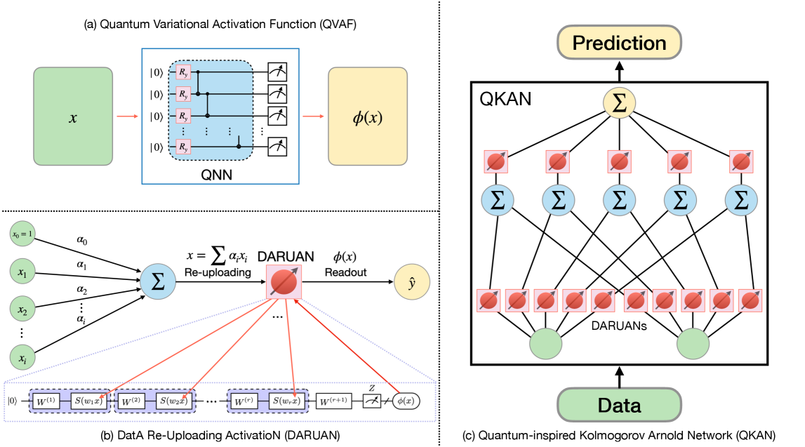
Figure 1: Schematic overview of the proposed quantum machine learning models. (a) A quantum neural network (QNN) serves as a variational activation function (VAF), where an input $x$ is processed by a quantum circuit to yield the output $\phi(x)$. (b) Specifically, we implement VAFs within a perceptron using a single-qubit data re-uploading circuit with trainable data pre-processing weights $w_{\ell}$ in the $\ell$-th encoding block $S(w_{\ell}x)$. The $\ell$-th parameterized unitary is $W^{(\ell)}=W^{(\ell)}(\bm{\theta}_{\ell})$, where $\bm{\theta}_{\ell}$ is the set of trainable parameters in $W^{(\ell)}$. The aggregated input $x=\sum\alpha_{i}x_{i}$ is repeatedly uploaded into each data encoding block, and the measurement outcome of the parameterized circuit defines the activation function. (c) We further incorporate data re-uploading activations into the structure of Kolmogorov-Arnold networks (KANs), treating each edge’s activation as the output of a distinct quantum circuit. Post-activation values are summed according to a predefined pattern to yield subsequent layer outputs, ultimately resulting in a quantum-inspired Kolmogorov-Arnold network (QKAN).

Quantum computing (QC) and quantum machine learning (QML) represent rapidly evolving interdisciplinary research frontiers that leverage quantum mechanical principles to perform computation (Biamonte et al., 2017; Dunjko et al., 2016; Chen and Liang, 2025). In QML, a central theme involves encoding classical data into high-dimensional Hilbert spaces using quantum states, harnessing the advantages of superposition, coherence, and entanglement to enable efficient learning from complex datasets (Biamonte et al., 2017; Ciliberto et al., 2018; Schuld and Killoran, 2019; Phillipson, 2020; Meyer et al., 2023; Liu et al., 2024a; Devadas and T, 2025).

Among the primary models in QML are variational quantum circuits (VQCs) which serve as quantum analogues of classical neural networks (Farhi and Neven, 2018; Chen et al., 2020). VQCs encode input data via structured ansatz and optimize parameterized gates using classical algorithms (Schuld et al., 2021; Pérez-Salinas et al., 2020). VQCs are the foundation of the hybrid quantum-classical machine learning paradigms (Mari et al., 2020) and widely regarded as one of the most promising routes toward demonstrating quantum advantage in near-term applications (Jerbi et al., 2023).

In parallel, advances in classical machine learning have spotlighted the use of learnable variational activation functions (VAFs), particularly through the development of Kolmogorov-Arnold networks (KANs) (Liu et al., 2024c). Inspired by the Kolmogorov-Arnold representation theorem (KART), KANs extend the concept of classical multilayer perceptrons (MLPs) by replacing fixed nonlinearities with learnable VAFs at each edge and performing summation at each node. This approach has yielded improvements in both predictive accuracy and interpretability and has shown promising results across a broad range of tasks including computer vision (Li et al., 2024a; Abd Elaziz et al., 2024; Xingyi Yang, 2025) and time series forecasting (Vaca-Rubio et al., 2024; Xu et al., 2024b; Genet and Inzirillo, 2024). More researches have explored VAF implementations in KAN using Chebyshev polynomials (SS et al., 2024), wavelets (Bozorgasl and Chen, 2024; Seydi, 2024b), Fourier series (Xu et al., 2024a), radial basis functions (Li, 2024), and other function bases (Howard et al., 2024; Ta, 2024; Aghaei, 2024; Seydi, 2024a; Xingyi Yang, 2025). Liu et al. (2024b) further enriched the expressivity of KANs by incorporating multiplicative interactions at the nodes.

Recent studies have established that VQCs can approximate any analytic function (Mitarai et al., 2018), and under certain conditions, even arbitrary continuous functions (Schuld et al., 2021; Yu et al., 2022, 2024b). Nevertheless, much of the QML literature has focused on data encoding strategies rather than function approximation. Notably, the ability of VQCs to learn even a single-variable function $f(x)$ already exceeds classical capabilities, motivating new approaches that leverage this expressive potential (Wach et al., 2023).

In this work, we propose to use VQCs not as standalone learners but as VAFs within classical or hybrid architectures, introducing a novel framework termed quantum variational activation functions (QVAFs). As single-qubit data re-uploading circuit itself is classically efficiently simulable and powerful enough to learn an univariate function (Pérez-Salinas et al., 2020; Schuld et al., 2021; Yu et al., 2022), we instantiate QVAFs using single-qubit circuits and name this model DatA Re-Uploading ActivatioN (DARUAN). The term “daruan” is derived from a Chinese traditional plucked string instrument renowned for its deep and coherent, mellow tone.

To demonstrate the broader applicability of this concept, we further extend DARUAN to Quantum-inspired Kolmogorov-Arnold Networks (QKANs), where DARUAN modules serve as quantum-inspired VAFs within the KAN framework. A schematic illustration of the QVAF, DARUAN, and QKAN architectures is provided in Figure˜1 respectively.

We theoretically analyze the frequency spectrum, $C^{m}$-norm approximation error and parameter estimation of single-qubit data re-uploading circuits in QKANs with and without trainable data pre-processing weights. We demonstrate that when trainable weights are incorporated into the data pre-processing phase, we can achieve an exponential reduction in parameter size compared to the classical Fourier-series-based KAN.

We empirically validate our proposed models on a variety of tasks, including regression, classification, and generative modeling. While QKANs and KANs show promising results, we notice that the number of parameters increases quadratically with the input and output dimensions, a challenge inherent to both architecture. To mitigate this issue, we present an adaptive algorithm, hybrid QKAN (HQKAN), that dynamically reduce parameter counts, thereby improving scalability.

While QKANs and DARUANs utilize only a single qubit in each activation, this approach enables efficient simulation on classical computers. By leveraging the concept of distributed machine learning on GPUs, our models can effectively handle large-scale training tasks, including the training of large language models (LLMs).

Our results show that QKANs, with appropriate architectural refinements, match or surpass the performance of classical KANs and MLPs while using significantly fewer parameters and computational resources. By integrating quantum circuit designs into VAFs, the QVAF and DARUAN frameworks offer a compelling avenue toward practical, resource-efficient quantum machine learning.

2 Results

2.1 The Quantum Variational Activation Function

The concept of VAFs has recently gained attention in classical machine learning, where the activation functions within neural networks are no longer fixed but instead treated as trainable parameters $\bm{\theta}\in\mathbb{R}^{d}$.

$$\phi_{\bm{\theta}}\colon\mathbb{R}\longrightarrow\mathbb{R},\quad x\mapsto\phi_{\bm{\theta}}(x).$$ (2.1)

This approach enhances a network’s expressivity by allowing it to learn the most suitable nonlinear transformations from data, leading to improvements in accuracy, convergence, and generalization performance (Molina et al., 2019; Apicella et al., 2021; Liu et al., 2024c). Parametric ReLU (PReLU)(He et al., 2015) and Swish(Ramachandran et al., 2017) are two representative examples, where slope or gating parameters are learned during training. More flexible formulations include adaptive piecewise linear (APL) units (Agostinelli et al., 2015), kernel activation functions (Scardapane et al., 2019), and spline-based activations (Liu et al., 2024c), all of which treat activation function as learnable entities.

Inspired by this classical paradigm, we propose a quantum analogue: the QVAF. In this framework, the role of an activation function is replaced with variational quantum circuit, which processes the input and produce a nonlinear transformation derived from quantum measurement. In general, a QVAF is defined as:

$$\phi_{\bm{\theta}}(x)=\langle 0|U(x;\boldsymbol{\theta})^{\dagger}\mathcal{M}U(x;\boldsymbol{\theta})|0\rangle,$$ (2.2)

where the input $x\in\mathbb{R}$ is encoded via data re-uploading or angle encoding into qubits, $U(x;\boldsymbol{\theta})$ is a trainable unitary circuit, $\mathcal{M}$ is an Hermitian observable with the norm $\lVert\mathcal{M}\rVert\leq 1$, and the expectation value yields a bounded nonlinear function.

The expressive power of QVAFs stems from their ability to generate highly nonlinear, tunable transformations even in low-depth, single-qubit circuits (Schuld et al., 2021; Mitarai et al., 2018). Moreover, since these activations are inherently smooth and bounded, they are particularly well-suited for stable training. Prior work has shown that VQCs are capable of approximating any analytic function (Mitarai et al., 2018) and even arbitrary continuous functions under certain conditions (Schuld et al., 2021). This positions QVAFs as universal approximators, analogous to classical VAFs but with access to quantum-enhanced feature spaces.

Recent efforts such as variational quantum splines (Inajetovic et al., 2023) and quantum-inspired activation circuits in hybrid convolutional networks (Li et al., 2024b) have demonstrated the potential of empirical viability of QVAFs on both synthetic and real-world data.

To implement QVAFs in practice and facilitate their integration into layered network architectures, we introduce DARUAN leveraging the data re-uploading circuit framework (Pérez-Salinas et al., 2020) to construct a scalable quantum-inspired activation layer with multiple repetitions and trainable pre-processing weights in a single qubit. Each block consists of a data encoding alternated with trainable unitaries, forming a variational circuit capable of approximating smooth periodic and non-periodic functions. The output is obtained via measurement of a Pauli observable (typically $\sigma_{z}$ in computational basis) and is used as the nonlinear transformation applied to the neuron output. In Figure˜1(b), DARUAN acts as VAF in a perceptron where the classical data is re-uploaded multiple times to data re-uploading variational quantum circuit and readout the expectation value of the data re-uploading circuit as final output.

Importantly, DARUAN supports architectural flexibility through a concept we term layer extension, which progressively increases the number of re-uploading repetitions, where we discuss the details in Section˜4. In our latter part of the experiments, this design allows the model to scale its expressivity on demand while preserving previously learned features. Layer extension addresses the challenge of optimizing deep quantum circuits, which are notoriously difficult to optimize (McClean et al., 2018). The simplicity of DARUAN, which relies solely on single-qubit circuits, makes it well-suited for implementation on current noisy intermediate-scale quantum (NISQ) devices. State-of-the-art trapped-ion platforms have achieved single-qubit gate error rates at the $10^{-7}$ level (Smith et al., 2025), while superconducting architectures have reached $10^{-5}$ (Rower et al., 2024), ensuring that DARUAN is experimentally feasible on current NISQ hardware. At the same time, our method is highly efficient to simulate on modern GPUs and multi-node high-performance computing (HPC) clusters, enabling large-scale benchmarking and seamless integration into GPT architectures. This dual capability underscores both near-term hardware implementability and practical scalability in classical simulation, while preserving competitive expressive power across both settings.

Furthermore, hybrid models leveraging QVAFs benefit from a form of exponential compression: a QVAF can implicitly encode a large number of frequency modes. This suggests that QVAFs serve not only as activation functions but also as compact feature extractors within hybrid quantum-classical architectures.

QVAFs open a promising path toward expressive, trainable nonlinearities in QML. They provide both theoretical richness and practical flexibility, enabling efficient approximation capabilities in low-resource quantum settings.

2.2 QKAN architecture

Building upon the insights from KANs (Liu et al., 2024c) and the expressive power of DARUAN, we introduce the QKANs. In this architecture, each activation function traditionally implemented via B-spline interpolation in KANs is replaced by DARUAN, a single-qubit data re-uploading variational quantum circuit, yielding a compact and trainable nonlinearity.

The central idea of QKANs is to harness the mathematical nature of Fourier-like expansion properties of data re-uploading quantum circuits, which approximate target functions via tunable superpositions of frequency components (Schuld et al., 2021). These circuits serve as QVAFs, enabling QKANs to learn highly expressive mappings using significantly fewer parameters than classical VAFs. While KANs approximate activation functions through B-spline bases with grid size $G$, QKANs estimate analogous Fourier coefficients through a parameter-efficient quantum circuit with a relative small number of data re-uploading repetitions $r$.

Each QKAN layer is constructed from a collection of single-qubit DARUANs organized in a feedforward structure. For a layer $l$ with $n_{l}$ input nodes and $n_{l+1}$ output nodes, the layer is defined as:

$$\Phi_{l}=\{\phi_{l,j,i}\},~i=1,2,\ldots,n_{l},~j=1,2,\ldots,n_{l+1};$$ (2.3)

$$\phi_{l,j,i}(x_{l,i})=\bra{0}U(x_{l,i},\bm{\theta}_{l,j,i})^{\dagger}\mathcal{M}U(x_{l,i},\bm{\theta}_{l,j,i})\ket{0};$$ (2.4)

$$x_{l+1,j}=\sum_{i=1}^{n_{l}}\phi_{l,j,i}(x_{l,i}),$$ (2.5)

where $i,j$ are indexes of input and output node respectively, $U(x;\bm{\theta})$ denotes the data re-uploading unitary circuit with trainable parameters $\bm{\theta}$, and $\mathcal{M}$ is the Pauli observable measured to obtain the circuit output. The final model is obtained by composing these layers:

$$\bm{y}=\text{QKAN}(\bm{x})=(\Phi_{L}\circ\Phi_{L-1}\circ\cdots\circ\Phi_{2}\circ\Phi_{1})(\bm{x}),$$ (2.6)

where the output is bounded within $[-n_{L-1},n_{L-1}]^{n_{L}}$ due to the nature of quantum expectation values.

QKANs offer both theoretical and practical advantages in terms of approximation capacity and parameter efficiency. From a complexity perspective, the number of parameters required for a QKAN with depth $L$, width $N$, and repetition count $r$ scales as $\mathcal{O}(N^{2}Lr)$. In contrast, KANs demand $\mathcal{O}(N^{2}LG)$ parameters, where $G$ is the number of spline grid points. As detailed in Theorem 2.2, the number of Fourier modes grows exponentially with $r$, and therefore, a small $r$ suffices to yield a significant reduction in parameters compared to classical grid-based and Fourier-based approaches.

Consequently, QKANs inherit the shallow architecture and structured interpretability of KANs while achieving parameter efficiency and enhanced expressivity through quantum-inspired VAF, DARUAN. As such, they form a promising and scalable approach for realizing compact, data-efficient, and interpretable models in QML.

2.3 Theoretical Analysis of QKAN

We analyze the architectural design of QKAN and establish its quantum advantages over classical KAN. First, we present an approximation theory for KART (Theorem˜2.1) based on Fourier series, extending Theorem 2.1 of Liu et al. (2024c) from the case of B-spline basis functions. We then investigate the frequency spectrum, $C^{m}$-norm approximation error, and parameter estimation for the Fourier series representation of single-qubit data re-uploading circuits within QKAN, as formalized in Theorem˜2.2.

Theorem 2.1 (Approximation Theory with Fourier Series, modified from Theorem 2.1 in Liu et al. (2024c)).

Let $\bm{}x=(x_{1},x_{2},\dots,x_{n}).$ Suppose that a function $f(\bm{x})$ admits a representation:

$$f(x)=(\Phi_{L}\circ\Phi_{L-1}\circ\cdots\circ\Phi_{2}\circ\Phi_{1})(\bm{x}),$$ (2.7)

where each $\Phi_{l,j,i}$ is $(k+1)$-times continuously differentiable. Then, there exists a constant $C$ depending on $f$ and its representation such that we have the following approximation bound in terms of the highest frequency $K$ in the Fourier series: there exist trigonometric polynomial approximations $\Phi^{K}_{l,i,j}$ such that for any integer $m$ with $0\leq m\leq k$, we have the bound:

$$\left\|f-(\Phi^{K}_{L}\circ\Phi^{K}_{L-1}\circ\cdots\circ\Phi^{K}_{1})(\bm{x})\right\|_{C^{m}}\leq CK^{-(k+1-m)},$$ (2.8)

where the $C^{m}$-norm approximation error measures the magnitude of derivatives up to order $m$:

$$\|g\|_{C^{m}}=\max_{|\beta|\leq m}\sup_{\bm{x}\in[0,1]^{n}}\left|D^{\beta}g(\bm{x})\right|,$$ (2.9)

and $D^{\beta}$ denotes the partial derivative of order $\beta$.

The proof is provided in Section˜A.1.

Remark 1.

In Theorem˜2.1, by changing the B-splines in Theorem 2.1 of Liu et al. (2024c) to Fourier series with the highest frequency $K$, we derive the approximation error bound. This shows the approximation error in the $C^{m}$-norm decays at the rate $\mathcal{O}(K^{-(k+1-m)})$ as the number of Fourier modes $2K$ increases. The approximation accuracy is controlled by the grid size $G$ in B-splines or the highest frequency $K$ in the Fourier series.

Theorem 2.2 (Spectrum expansion and approximation error of QKAN with linear layer).

Fix an integer $k\!\geq\!0$ and a target function $f\in C^{k+1}[0,1]$. For any depth $r\!\geq\!1$, consider two single-qubit data re-uploading circuits:

(A) Baseline (Un-weighted).

$$U(x) =W^{(r+1)}\bigl[S(x)\,W^{(r)}\bigr]\cdots\bigl[S(x)\,W^{(1)}\bigr],$$

$$S(x) =e^{-ixH},$$

where $W^{(\ell)}=W^{(\ell)}(\bm{\theta}_{\ell})$ is the $\ell$-th parameterized unitary with $\bm{\theta}_{\ell}$ being the set of trainable parameters and $H=\frac{1}{2}\sigma_{j}$ is the Hermitian generator and $\sigma_{j}\in\{\sigma_{x},\sigma_{y},\sigma_{z}\}$.

(B) With a classical linear layer. Let $\bm{\omega}=(w_{1},\dots,w_{r})^{\!\top}\in(0,\infty)^{r}$ and set

$$U_{\bm{\omega}}(x) =W^{(r+1)}\prod_{\ell=r}^{1}\bigl[S(w_{\ell}x)\,W^{(\ell)}\bigr],$$

$$S(w_{\ell}x) =e^{-iw_{\ell}xH}.$$

Define the model outputs

$$f_{A}(x) =\langle 0|U^{\dagger}(x)\mathcal{M}U(x)|0\rangle,$$

$$f_{B}(x) =\langle 0|U_{\bm{\omega}}^{\dagger}(x)\mathcal{M}U_{\bm{\omega}}(x)|0\rangle.$$

1. Baseline spectrum.  $f_{A}$ is a trigonometric polynomial $f_{A}(x)=\sum_{\alpha=-r}^{r}c_{\alpha}e^{i\alpha x},$ hence the number of distinct non-zero frequencies is $|\Omega_{A}|=2r.$

2. Linear-layer expansion.  $f_{B}$ has spectrum

   $$\Omega_{B}=\left\{\!\sum_{\ell=1}^{r}m_{\ell}w_{\ell}\;\Bigm|\;m_{\ell}\in\{-1,0,1\}\right\}.$$

   The number of distinct non-zero frequency satisfies $1\leq|\Omega_{B}|\leq(3^{r}-1).$

3. $C^{m}$-norm approximation error.  For $0\leq m\leq k$

   $$\|f-f_{A}\|_{C^{m}} \leq C_{f}\,K_{A}^{-(k+1-m)},\quad K_{A}:=r,$$

   $$\|f-f_{B}\|_{C^{m}} \leq C_{f}\,K_{B}^{-(k+1-m)},\quad K_{B}:=\sum_{\ell=1}^{r}w_{\ell}.$$

4. Parameter efficiency vs. Fourier-series-based KAN.  A classical Fourier-series-based KAN requires $M=\Theta\!\bigl(\varepsilon^{-1/(k+1-m)}\bigr)$ parameters to reach error $\varepsilon$ in $C^{m}$ norm. By choosing the geometric weights $w_{\ell}=2^{\ell-1}$, we have $K_{B}=2^{r}-1$ and

   $$\|f-f_{B}\|_{C^{m}}\leq C_{f}\,2^{-r(k+1-m)}.$$

   Solving $C_{f}\,2^{-r(k+1-m)}=\varepsilon$ gives

   $$r=\left\lceil\frac{\log_{2}(C_{f}/\varepsilon)}{k+1-m}\right\rceil=\Theta\!\big(\log\tfrac{1}{\varepsilon}\big),$$

   so the total number of trainable parameters is $\Theta(\log\tfrac{1}{\varepsilon})$, an exponential reduction compared to Fourier-series-based KAN.

The proof is provided in Section˜A.2.

In Theorem˜2.2(a), we show that the maximum spectrum size of an unweighted data re-uploading circuit grows only linearly with $r$. To overcome this limitation, DARUAN and QKAN introduce trainable weights that exponentially expand and reshape the dynamically controllable frequency spectrum, as formalized in Theorem˜2.2(b) and also employed in prior works (Zhao et al., 2024; Yu et al., 2022).

Together with Theorem˜2.1, these results establish a Fourier-series-based approximation theory, where the error bound is determined by the maximum frequency $K_{B}$. By exploiting the exponentially large Fourier spectrum, we demonstrate the expressive power of QKAN, as stated in Theorem˜2.2(c) and (d).

A central challenge, however, is the exponential vanishing-gradient problem (McClean et al., 2018) in large quantum models. QKAN addresses this by enabling dynamical frequency spectrum expansion during training through the parameter $r$. This stands in contrast to classical KANs, where functional granularity is adjusted by the grid size $G$ and refined through grid extension. In QKANs, the frequency increases exponentially during training with learnable circuit depth, enabling gradual fine-tuned global feature through layer extension. Therefore, we employ the layer extension strategy, introduced earlier and elaborated in the Section˜4, as a practical solution to mitigate vanishing gradients while preserving expressive power.

2.4 Numerical Results

In this section, we assess the versatility and effectiveness of QKANs by simulating various tasks, including regression, classification, and generative modeling. Overall, our experiments demonstrate that QKAN consistently outperforms classical KAN and MLP baselines across tasks. In regression benchmarks, QKAN achieves up to an order-of-magnitude reduction in approximation error with significantly fewer parameters. For classification tasks, QKANs and HQKANs consistently surpass classical KANs and MLP baselines in both top-1 and top-5 accuracy, while HQKANs achieves this with substantially fewer parameters. In generative modeling, HQKAN integrated into GPT-2 obtains lower perplexity and reduced training time and computational resources compared to MLP counterparts. These results establish QKAN as a scalable and hardware-efficient alternative to classical architectures, with strong potential for near-term and large-scale quantum-classical hybrid applications. Unless otherwise specified, the following results are obtained on a personally available NVIDIA RTX 4090 GPU. Detailed setups for each task are provided in the Section˜4.

We begin with a regression task focused on function fitting. Previous studies have demonstrated that KANs outperform MLPs in various regression problems, including multivariate function fitting and solving partial differential equations (PDEs) (Liu et al., 2024c, b). In particular, KANs have shown strong performance in symbolic expression recovery (Yu et al., 2024a; Liu et al., 2024b). To investigate the robustness of QKAN and its potential for real-world applications, we prepare a regression dataset with added noise in both training and testing labels.

We start with heuristic function fitting, where the hidden layers and hidden nodes are manually specified. As a simple example, we consider fitting the function $f(x)=J_{0}(20x)$, where $J_{0}$ is a Bessel function that $J_{0}(x)={\sin{(x)}}/{x}$, using QKAN and KAN with a heuristic QKAN (KAN) shape $\left[1,1\right]$. The training label is subject to a Gaussian error with a standard deviation of 0.1. The results are shown in Figure˜2, where QKAN yields a smoother approximation to the noisy data, while KAN captures more localized features, which in this case correspond to the noise.

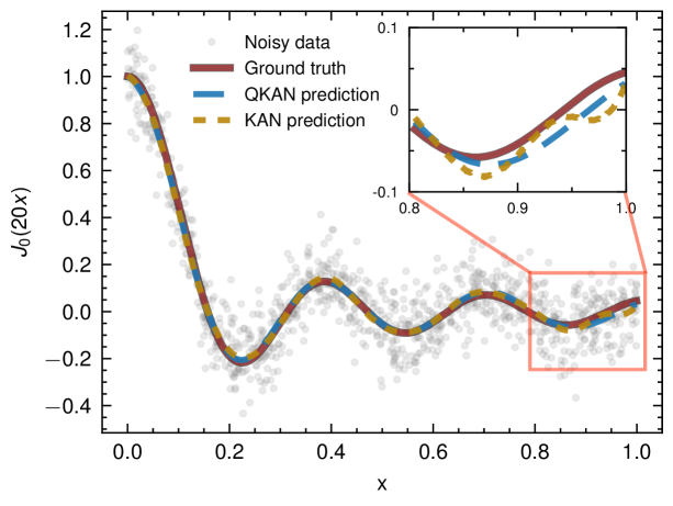
Figure 2: Function fitting with noise using QKAN and KAN. The target function is $f(x)=J_{0}(20x)$, fitted with noisy data. Both QKAN and KAN use a shape of $\left[1,1\right]$. The QKAN prediction exhibits smoother behavior compared to KAN which tends to overfit local noise features.

To further assess model performance, we conduct more complex heuristic function fitting experiments using the QKAN (KAN) shapes suggested in Liu et al. (2024c). We report the average of the best performance across five random seeds in Table˜1, and summarize the best test loss and parameter sizes for QKANs and KANs in Table˜2.

Table 1: Heuristic noisy function regression. We select 10 functions in Feynman dataset (Udrescu and Tegmark, 2020; Udrescu et al., 2020) and each function is represented by a dimensionless formula with its variables. Moreover, we randomly sample the data with 10 % noise level and 1000 training, 1000 testing data points for each function. Each function has inputs within the range of $\left[0,1\right]$. The shapes of QKAN/KAN are represented by the number of hidden nodes in each layer. The performance is measured by the root mean square error (RMSE) of the predicted outputs compared to the test data. The best performance is highlighted in bold while the second is labeled with underline. The results show that QKAN outperforms KAN and MLP in most cases, demonstrating the effectiveness of the QKAN architecture in noisy function regression tasks.

Feynman eq.	Dimensionless formula	Variables	QKAN/KAN shape	QKAN	KAN	MLP
I.12.11	$1+a\sin{\theta}$	$a,\theta$	[2, 2, 1]	$\mathbf{1.1911\times 10^{-1}}$	$\underline{1.210\times 10^{-1}}$	$1.3877\times 10^{-1}$
I.29.16	$\sqrt{1+a^{2}-2a\cos{(\theta_{1}-\theta_{2})}}$	$a,\theta_{1},\theta_{2}$	[3, 2, 3, 1]	$\mathbf{1.4452\times 10^{-1}}$	$\underline{1.4658\times 10^{-1}}$	$3.1924\times 10^{-1}$
I.40.1	$n_{0}e^{-a}$	$n_{0},a$	[2, 2, 1, 1, 1, 2, 1]	$\underline{1.0391\times 10^{-1}}$	$\mathbf{3.8206\times 10^{-2}}$	$7.9577\times 10^{-1}$
I.50.26	$\cos{a}+\alpha\cos^{2}{a}$	$a,\alpha$	[2, 2, 3, 1]	$\underline{1.1680\times 10^{-1}}$	$1.1858\times 10^{-1}$	$\mathbf{1.1351\times 10^{-1}}$
II.2.42	$(a-1)b$	$a,b$	[2, 2, 1]	$\mathbf{2.4054\times 10^{-2}}$	$\underline{2.4416\times 10^{-2}}$	$4.3203\times 10^{-1}$
II.6.15a	$\frac{1}{4\pi}c\sqrt{a^{2}+b^{2}}$	$a,b,c$	[3, 2, 1, 1]	$\underline{3.1332\times 10^{-3}}$	$\mathbf{3.0759\times 10^{-3}}$	$7.9275\times 10^{-3}$
II.35.18	$\frac{n_{0}}{\exp{(a)}+\exp{(-a)}}$	$n_{0},a$	[2, 1, 1]	$\mathbf{2.1154\times 10^{-2}}$	$\underline{2.1275\times 10^{-2}}$	$1.1086\times 10^{-1}$
II.36.38	$a+\alpha b$	$a,b,\alpha$	[3, 2, 1]	$\mathbf{7.3153\times 10^{-2}}$	$\underline{8.0143\times 10^{-2}}$	$1.6865\times 10^{-1}$
III.10.19	$\sqrt{1+a^{2}+b^{2}}$	$a,b$	[2, 1, 1]	$\mathbf{1.2415\times 10^{-1}}$	$\underline{1.2443\times 10^{-1}}$	$1.4845\times 10^{-1}$
III.17.37	$\beta(1+\alpha\cos{\theta})$	$\alpha,\beta,\theta$	[3, 3, 1]	$\mathbf{6.8907\times 10^{-2}}$	$\underline{7.0658\times 10^{-2}}$	$3.3668\times 10^{-1}$

Table 2: Comparison of QKAN and KAN in heuristic noisy function regression. Continue from Table˜1, we report the number of parameters and RMSE loss of QKAN and KAN models. The best performance is highlighted in bold. The results show that QKAN outperforms KAN while requiring 30 % fewer parameters in average.

Feynman	QKAN		KAN
equation	RMSE loss	# Params	RMSE loss	# Params
I.12.11	$\bm{1.1911\times 10^{-1}}$	96	$1.210\times 10^{-1}$	135
I.29.16	$\bm{1.4452\times 10^{-1}}$	240	$1.4658\times 10^{-1}$	336
I.40.1	$1.0391\times 10^{-1}$	192	$\bm{3.8206\times 10^{-2}}$	272
I.50.26	$\bm{1.1680\times 10^{-1}}$	208	$1.1858\times 10^{-1}$	292
II.2.42	$\bm{2.4054\times 10^{-2}}$	96	$2.4416\times 10^{-2}$	135
II.6.15a	$3.1332\times 10^{-3}$	144	$\bm{3.0759\times 10^{-3}}$	202
II.35.18	$\bm{2.1154\times 10^{-2}}$	48	$2.1275\times 10^{-2}$	68
II.36.38	$\bm{7.3153\times 10^{-2}}$	128	$8.0143\times 10^{-2}$	179
III.10.19	$\bm{1.2415\times 10^{-1}}$	48	$1.2443\times 10^{-1}$	68
III.17.37	$\bm{6.8907\times 10^{-2}}$	192	$7.0658\times 10^{-2}$	268

As shown in Table˜1, QKAN consistently outperforms both KAN and MLP baselines in the majority of cases, achieving the lowest test RMSE on 7 out of the 10 benchmark equations. This trend demonstrates that QVAF in QKAN effectively captures complex patterns in noisy regression tasks. In the remaining three cases, QKAN still ranks second, with performance closely matching or slightly trailing that of the best-performing baseline. The results suggest that QKAN’s expressive feature mappings are especially well-suited for capturing high-frequency or compositional structures, where classical models tend to underperform.

Table˜2 further reveals that QKAN models not only deliver superior or comparable performance but also achieve this with significantly fewer parameters. On average, QKAN uses about 30% fewer parameters than KAN while maintaining or improving generalization accuracy. This parameter efficiency is especially advantageous in scenarios with limited model capacity or deployment constraints.

However, in most scenarios the underlying functional form is unknown a priori. To evaluate model robustness under such uncertainty, we extend our study to a diverse suite of 66 symbolic expressions drawn from the Feynman dataset (Udrescu and Tegmark, 2020; Udrescu et al., 2020), each input normalized to the unit hypercube and output subject to 10% additive noise. For each equation, we optimize QKAN, KAN and MLP architectures over hidden‐layer depths as described in Method Section, and record the lowest test RMSE attained across five random seeds.

Figure˜5 displays these best‐case losses on a logarithmic scale, with the total number of trainable parameters annotated for both QKANs and KANs. Notably, QKAN achieves the lowest RMSE on over 80% of the benchmark equations, despite employing on average 30% fewer parameters than classical KAN. In the minority of cases where KAN marginally outperforms, the QKAN remains competitive, often within the same order of magnitude, while retaining its parameter‐efficiency advantage. By contrast, standard MLPs exhibit rapidly deteriorating generalization as equation complexity increases, underscoring the critical role of structured feature embeddings in noisy symbolic regression.

These results substantiate the dual strengths of QKAN: QVAF and DARUAN not only enhance expressivity in the absence of exact analytic priors but also deliver substantial parameter savings. Consequently, QKAN represents a compelling approach for data‐driven discovery and modeling in scientific applications where both accuracy and resource constraints are paramount. The quantum-enhanced architecture provides both improved generalization and model compactness, highlighting its potential for broader applications in data-driven scientific modeling.

To evaluate the expressive power and scalability of QKANs beyond function regression, we investigate their performance on image classification tasks. We consider three standard benchmarks—MNIST (Deng, 2012), CIFAR-10, and CIFAR-100 (Krizhevsky and Hinton, 2009)—and use a hybrid architecture where a convolutional neural network (CNN) is followed by a fully connected network (FCN). In our setup, the FCN is instantiated using either an MLP, a KAN, or a QKAN, enabling a direct comparison across model families with identical convolutional backbones.

Table 3: Performance of different models on MNIST, CIFAR-10, and CIFAR-100 datasets. The top-1, top-5 test accuracy and the parameter size of each model. The second column indicates the parameter size of CNN shared by all models.

Model	(CNN)	CNN+MLP			CNN+KAN(G=10)			CNN+QKAN(r=3)			CNN+HQKAN
Training	CNN	Top-1	Top-5	MLP	Top-1	Top-5	KAN	Top-1	Top-5	QKAN	Top-1	Top-5	HQKAN
dataset	# Params	Accuracy (%)		# Params	Accuracy (%)		# Params	Accuracy (%)		# Params	Accuracy (%)		# Params
MNIST	1,084	97.9	100.0	850	97.7	100.0	1,500	98.0	100.0	800	95.9	99.7	222
CIFAR-10	56,320	71.4	97.8	41,802	68.4	97.4	39,900	68.8	97.0	21,280	71.6	97.9	14,370
CIFAR-100	56,320	39.8	69.4	86,948	40.6	70.4	384,000	41.2	70.0	204,800	39.9	70.6	32,636

Table˜3 reports the top-1 and top-5 classification accuracies together with the parameter counts of the FCN components. Top-1 accuracy measures the proportion of test samples for which the model’s single most confident prediction coincides with the true label, whereas top-5 accuracy considers a prediction correct if the ground-truth label is contained within the top five highest probabilities.

On MNIST, all models achieve high accuracy, with CNN+QKAN attaining the highest top-1 accuracy of 98.0% and perfect top-5 accuracy using only 800 parameters in the FCN. In contrast, CNN+MLP and CNN+KAN require significantly more parameters (850 and 1,500, respectively) to achieve comparable accuracy. This suggests that QKAN can achieve strong performance with minimal parameter overhead, even on simple tasks.

The advantage of QKAN becomes more evident on CIFAR-10, where CNN+QKAN achieves the comparable top-1 and top-5 accuracies (68.8% and 97.0%, respectively) while requiring nearly half the parameters of CNN+KAN (21,280 vs. 39,900). CNN+MLP, despite having a similar parameter count to KAN, doesn’t outperform in both metrics. This highlights QKAN’s superior parameter efficiency and generalization capacity.

For the more challenging CIFAR-100 dataset, CNN+QKAN achieves the highest top-1 accuracy (41.2%), outperforming CNN+KAN and CNN+MLP while using fewer parameters than CNN+KAN. Notably, CNN+KAN and CNN+QKAN require a substantial number of parameters due to their linear scaling with output size, 384k and 205k respectively, posing limitations for practical deployment.

To address the scalability constraints of QKAN and KAN on high-dimensional tasks, we introduce Hybrid QKAN (HQKAN), which incorporates two additional fully connected layers to form an autoencoder-like structure around a compact QKAN core. By compressing features into a small latent space, HQKAN leverages QKAN’s expressivity while significantly reducing parameter count.

As demonstrated in Table˜3, HQKAN achieves competitive accuracy with an order-of-magnitude reduction in parameters. For example, on CIFAR-100, HQKAN attains a top-5 accuracy of 70.6% using only 32,636 parameters, compared to 86,948 and 384,000 required by MLP and KAN models, respectively. On CIFAR-10, HQKAN not only outperforms both MLP and KAN in top-1 and top-5 accuracy but does so with the fewest parameters (14,370). This result underscores the practicality of HQKAN for memory- and compute-constrained environments.

Together, these results validate the efficacy and versatility of QKANs and HQKANs across classification tasks of varying complexity. They demonstrate that QVAFs, particularly in the single-qubit data re-uploading circuit, DARUAN, provide an expressive, scalable, and hardware-efficient approach to deep learning.

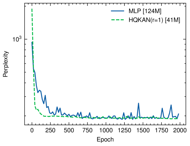
Figure 3: GPT-2 model trained on the WebText dataset (Radford et al., 2019), incorporating HQKAN and MLP layers. To further reduce parameter count and improve efficiency, we adopt the hybrid QKAN (HQKAN) strategy, where the input and output dimensions fed into QKAN are compressed via fully connected layers, forming an autoencoder-like bottleneck. This compression enables QKAN to operate effectively in a low-dimensional latent space with reduced overhead. Parameter sizes are indicated in square brackets. HQKAN achieves better perplexity performance than MLP while using only one-third of its parameters and the same training time, demonstrating the effectiveness of QKAN-based architectures for generative modeling on classical hardware.

We further evaluate the generative modeling capability of QKANs by integrating them into autoregressive language models, specifically the GPT-2 architecture. For preliminary testing, we utilize an open-source kan-gpt module (Ganesh, 2024). In this approach, we replace all the linear layers within the transformer blocks with HQKANs we introduced earlier in classification tasks to address the scaling problem in KANs architecture. Subsequently, we pretrain the resulting models on the WebText dataset (Radford et al., 2019).

Figure˜3 presents the perplexity curves during training of GPT-2 models equipped with MLP and HQKAN modules. Despite operating in a reduced-dimensional latent space, HQKAN consistently achieves superior convergence and reduced final perplexity compared to the MLP baseline. This is achieved while taking only one-third of the parameters and 30% less memory during training time.

To complement the generative modeling results presented in the main text, we provide detailed runtime and memory benchmarks for GPT-2 models incorporating QKAN-based components. In particular, we aim to assess the scalability of these models under large-batch training regimes, as large batch sizes have been shown to significantly improve performance in LLMs with scaling laws (Brown et al., 2020; Shuai et al., 2024).

Table˜4 summarizes the performance of various GPT-2 configurations on the WebText dataset. The top section of the table (above the second double midrule) evaluates models using the kan-gpt framework, where the linear layers in GPT-2 are replaced by HQKANs. Models marked with an asterisk (*) correspond to those visualized in Figure˜3 of the main text. We measure the iteration time and memory consumption for each methods.

The lower section of the table reports results for the KANsformer architecture (Xie et al., 2024), which integrates HQKAN modules directly into the feedforward layers of transformer blocks, with flash attention (Dao et al., 2022). Flash attention significantly reduces memory usage and improves speed. We report performance at various batch sizes to demonstrate the scalability and hardware compatibility of QKAN-based architectures under realistic training regimes.

Table 4: Performance comparison of GPT-2 models on the WebText dataset (Radford et al., 2019). This table presents the runtime and memory usage for various GPT-2 configurations equipped with QKAN-based modules. The top section (above the second double midrule) corresponds to models using the kan-gpt framework introduced in the main text, where all linear layers are replaced by HQKAN. The models marked with an asterisk (*) are those displayed in Figure˜3. Results include training speed (ms per iteration) and memory consumption. The lower section (below the second double midrule) reports large-scale results using the KANsformer (Xie et al., 2024) architecture with flash attention (Dao et al., 2022), which integrates HQKAN directly into the feed-forward network of transformer block instead of all linear layers. We benchmark across batch sizes and hardware configurations, including single- and multi-GPU setups with NVIDIA RTX 4090, V100S, H100, and H200 GPUs. These configurations demonstrate the scalability and practical feasibility of HQKAN-based models in both single- and distributed-training regimes.

Method	# Params	Batch size	Time/iter [GPU $\cdot$ ms]	Device memory
MLP-based GPT	124 M	*1	63 [RTX 4090 $\cdot$ ms]	6.5 GB
w/o flash atten.		48	4,536 [V100S $\cdot$ ms]	111 GB
HQKAN-gpt	41 M	*1	60 [RTX 4090 $\cdot$ ms]	4.1 GB
w/o flash atten.		48	4,648 [V100S $\cdot$ ms]	120 GB
MLP-based GPT	124 M	1	40 [RTX 4090 $\cdot$ ms]	4.7 GB
w/ flash atten.		10	252 [RTX 4090 $\cdot$ ms]	17.3 GB
		48	3,884 [V100S $\cdot$ ms]	81.2 GB
		320	6,400 [H100 $\cdot$ ms]	656 GB
		800	14,784 [H200 $\cdot$ ms]	1,340 GB
HQKANsformer	67 M	1	39.5 [RTX 4090 $\cdot$ ms]	3.8 GB
w/ flash atten.		10	240 [RTX 4090 $\cdot$ ms]	15.6 GB
		48	3,540 [V100S $\cdot$ ms]	73.6 GB
		320	5,760 [H100 $\cdot$ ms]	592 GB
		800	13,232 [H200 $\cdot$ ms]	1,224 GB

Table˜4 highlights the runtime and memory efficiency of HQKAN-based GPT-2 models. On a single RTX 4090, HQKAN achieves comparable speed to standard MLPs (60 ms vs. 63 ms per iteration), while reducing memory consumption by over 35% (4.1 GB vs. 6.5 GB). When scaled to 4$\times$V100S GPUs at batch size 48, HQKAN maintains efficiency with only marginal overhead (4,648 ms vs. 4,536 ms), despite a threefold reduction in model size (40M vs. 124M parameters). Nevertheless, the device memory consumption and training time reveal scaling limitations for the kan-gpt method, which restricts its practicality for very large models.

To address this issue, we turn to KANsformer architecture with flash attention, and the results are shown in the lower section of Table˜4. This architecture provides further memory savings and speed improvements, enabling scalability to larger training regimes. At large batch sizes (e.g., 320), HQKANsformer reduces device memory from 656 GB to 592 GB compared to MLP, while also lowering per-iteration time (6,400 ms vs. 5,760 ms on total H100 times). Even at batch size 800 on 16$\times$H200, HQKANsformer completes iterations with both 10% less memory and 10% less time, demonstrating its efficiency at scale. In summary, HQKANsformer effectively overcomes the scalability bottleneck of the kan-gpt approach, making it a practical solution for training foundation models at large scale.

Overall, the results demonstrate that HQKAN can serve as an effective, efficient, and scalable plug-and-play replacement for classical fully connected layers in generative transformer architectures. Its parameter efficiency and faster convergence open the door to practical quantum-inspired modeling in large-scale natural language processing tasks.

Additionally, to investigate the compatibility between quantum-inspired and classical KAN, we present a knowledge distillation method to transfer learned parameters from a trained QKAN to a corresponding KAN (see Section˜4.3 for details). This process enables QKANs to serve as a pretraining mechanism for KANs, potentially accelerating convergence and improving generalization in the classical regime.

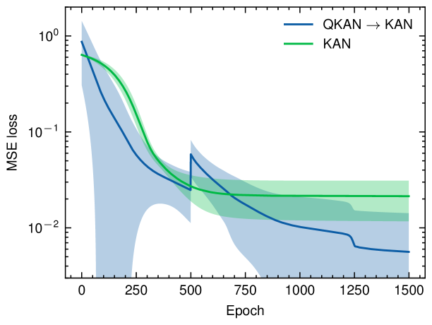
Figure 4: Knowledge distillation from QKAN to KAN. We consider the regression task $f(x,y)=\sin(e^{x}+y^{2})$. A QKAN is first trained for 500 epochs, after which its learned variational parameters are converted into B-spline coefficients and transferred into a KAN of matching architecture. Due to approximation errors during the conversion, a small loss shift is observed, which is corrected through continued training. The resulting QKAN-initialized KAN achieves a 70% reduction in test loss compared to a KAN trained from scratch, demonstrating the effectiveness of QKAN as a pretraining strategy for classical KAN.

We illustrate this approach with a toy function, $f(x,y)=\sin(e^{x}+y^{2})$, a nonlinear expression with compositional structure. As shown in Figure˜4, the QKAN is first trained close to convergence. Learned parameters are then converted into B-spline basis representations and transferred into a structurally matched KAN. Owing to spline approximation errors during the conversion, the KAN continues training for a limited number of epochs to fine-tune the inherited parameters.

This transfer approach yields a substantial performance gain: the transferred KAN achieves a 70% lower test loss compared to a baseline KAN trained from scratch under identical conditions. These results suggest that QKAN can serve as a powerful initialization strategy for KAN, effectively bootstrapping their learning via QVAFs.

3 Discussion

In this work, we introduce QKANs, a novel framework that integrates QVAFs into the classical KAN architecture. The core of this innovation lies in the design of QVAFs based on single-qubit data re-uploading circuits with trainable data pre-processing weights, which form the fundamental building blocks of our proposed DARUAN. DARUANs enable QKANs to approximate complex nonlinear mappings using significantly fewer parameters than traditional methods.

QVAFs offer a compelling perspective on variational quantum circuits, not only as data encoders or feature maps, but also as expressive, learnable nonlinearities embedded directly within neural architectures. By systematically organizing DARUAN into KAN layers, QKANs achieve an significant increase in functional expressivity per parameter with repetition, all while maintaining compatibility with the current hardware constraints of the NISQ era.

Our architecture not only preserves the structured interpretability of classical KANs but also enhances it with the power of quantum-inspired DARUAN. Empirical evaluations across regression, classification, and generative modeling tasks consistently show that QKANs outperform or rival both MLPs and traditional KANs, despite using fewer parameters and reduced training overhead.

To improve scalability and adaptability, we further introduced layer extension and HQKANs, allowing QKANs to flexibly accommodate various task complexities. These extensions broaden the model’s applicability without compromising its foundational design.

Though, due to the scope of this paper, which mainly focuses on the effectiveness of QKAN over classical KAN and MLP, we only benchmark QKAN with well-established models, instead of SOTA models on any particular task. Our results still verify that QKANs on par with MLP can serve as versatile backbone models across the spectrum of classical architectures—ranging from simple to complex—and consistently outperform classical KAN and MLP in terms of parameter efficiency with comparable or even better performance.

Importantly, QKANs are constructed from modular components that are readily implementable on current quantum devices, particularly leveraging single-qubit operations on NISQ devices (Smith et al., 2025; Rower et al., 2024). The possibility of transferring trained QKAN parameters to classical KANs enables a seamless hybridization of quantum and classical pipelines, offering practical benefits even before full-scale quantum hardware becomes widely accessible.

During the final stage of our manuscript revision, we became aware of several recent studies that also explore similar idea on QVAFs in KANs (Werner et al., 2025; Wakaura et al., 2025b, a). These works propose alternative VQC ansatz to serve as activation functions within the KAN framework, aligning with our formulation of QVAFs. However, a key distinction lies in the quantum resource requirements of these approaches. The aforementioned studies utilize multi-qubit circuits for their VQCs, which presents three major scalability challenges. First, the current limitations of quantum hardware, as well as the computational cost of classical quantum simulators, restrict the practical deployment of models with large qubit counts. Second, and more fundamentally, scaling up multi-qubit VQCs often leads to the emergence of barren plateaus, regions in the optimization landscape where the gradient vanishes exponentially with system size, making the training of large-scale quantum neural networks exceedingly difficult (McClean et al., 2018). Not to mention the fidelity, or error rate, of the two-qubit gate on NISQ devices is still challenging to realize deep circuits (Preskill, 2018; Singh et al., 2024; Smith et al., 2025), which leads to inscalability of the models. These limitations significantly hinder the scalability and practicality of multi-qubit QVAF-based KANs. Third, existing models still depend on access to real quantum hardware when scaling up, both during training and inference. Such real devices remain scarce and must typically be accessed through remote servers, introducing latency that is particularly detrimental for real-time tasks. In contrast, our proposed architecture, QKAN, employs only single-qubit data re-uploading circuits for its VAFs. These circuits are lightweight and efficient enough to be simulated on classical quantum simulators, thereby removing the reliance on real quantum devices during inference. This design not only enables efficient implementation on near-term quantum devices but also mitigates the risk of barren plateaus, providing a more scalable and robust path toward quantum-enhanced machine learning.

In summary, QKANs represent a significant step toward practical quantum-enhanced learning by integrating QVAFs and KANs within a scalable and computationally efficient framework. Crucially, this quantum-inspired design is already executable on classical quantum simulator and demonstrates readiness for large-scale deployment. Our work thus establishes QKANs as a bridge between interpretable classical architectures and future quantum acceleration, offering a blueprint for next-generation machine learning models.

4 Methods

This section provides a detailed overview of the core methods proposed and employed in this work.

4.1 Kolmogorov-Arnold Networks

KANs are designed to approximate multivariate functions using compositions of univariate functions and addition, establishing themselves as universal approximators with high interpretability and efficiency.

Kolmogorov-Arnold representation theorem.

KART (Kolmogorov, 1957) states that any multivariate continuous function $f(x_{1},\ldots,x_{N})$ can be represented as a finite composition of univariate functions and addition:

$$f(\bm{x})=\sum_{q=1}^{2N+1}\Phi_{q}\left(\sum_{p=1}^{N}\phi_{q,p}(x_{p})\right),$$ (4.1)

where $\phi_{q,p}:[0,1]\rightarrow\mathbb{R}$ and $\Phi_{q}:\mathbb{R}\rightarrow\mathbb{R}$ are continuous functions. While KART provides theoretical guarantees of universal approximation, the original functions can be non-smooth or hard to learn in practice (Girosi and Poggio, 1989; Poggio et al., 2020; Liu et al., 2024c), hence the need for parameterized and trainable alternatives.

Formalism of Kolmogorov-Arnold networks.

Liu et al. (2024c) introduced KANs as a practical realization of the KART, generalizing it to deep and wide architectures. Each activation in KANs is modeled as a learnable VAF parameterized by B-splines, which are piecewise polynomial functions capable of approximating any continuous function with arbitrary precision (Liu et al., 2024c; Douzette, 2017).

Formally, a KAN layer maps the output of the $l$-th layer to the $(l+1)$-th layer via:

$$x_{l+1,j}=\sum_{i=1}^{n_{l}}\phi_{l,j,i}(x_{l,i}),$$ (4.2)

where $\phi_{l,j,i}$ is the learnable univariate VAF connecting input node $i$ to output node $j$.

This can be expressed in matrix notation as:

$$\bm{x}_{l+1}=\Phi_{l}(\bm{x}_{l}),$$ (4.3)

$$\Phi_{l}=\begin{pmatrix}\phi_{l,1,1}(\cdot)&\phi_{l,1,2}(\cdot)&\cdots&\phi_{l,1,n_{l}}(\cdot)\\ \phi_{l,2,1}(\cdot)&\phi_{l,2,2}(\cdot)&\cdots&\phi_{l,2,n_{l}}(\cdot)\\ \vdots&\vdots&\ddots&\vdots\\ \phi_{l,n_{l+1},1}(\cdot)&\phi_{l,n_{l+1},2}(\cdot)&\cdots&\phi_{l,n_{l+1},n_{l}}(\cdot)\end{pmatrix}.$$ (4.4)

A KAN with depth $L$, width $N$, spline order $k$, and $G$ grid intervals requires $\mathcal{O}(N^{2}L(G+k))\sim\mathcal{O}(N^{2}LG)$ parameters (Liu et al., 2024c). This is comparable to MLPs with $\mathcal{O}(\mathcal{N}^{2}L)$ parameters for depth $L$ and width $\mathcal{N}$, but KANs typically require a significantly smaller width $N$, resulting in improved efficiency and generalization.

However, the computational cost of evaluating B-spline bases and rescaling grids can become a computational bottleneck in practice (Li, 2024). This motivates our exploration of quantum-inspired methods to replace spline-based activations with more efficient quantum circuit approximators.

4.2 Data Re-Uploading Circuits

To address the computational challenges associated with B-spline activations in classical KANs, we leverage the expressive power of VQCs, particularly through data re-uploading circuits (Pérez-Salinas et al., 2020).

Data re-uploading circuits encode classical inputs via repeated parameterized embeddings into quantum states, alternating with trainable unitaries. In general, for an implementation with $r$ repetitions with $n$-dimensional input $\bm{x}\in\mathbb{R}^{n}$, the circuit can be expressed as:

$$U(\bm{x},\bm{\theta})=W^{(r+1)}S(\bm{x})W^{(r)}\cdots S(\bm{x})W^{(1)},$$ (4.5)

where each $W^{(\ell)}$ is a trainable unitary and $S(\bm{x})$ is the data-encoding operation. A common instantiation is $S(\bm{x}\circ\bm{\omega}+\bm{\beta})$ with trainable parameters $\bm{\omega},\bm{\beta}\in\mathbb{R}^{n}$ (Zhao et al., 2024), where $\circ$ denotes a Hadamard product. In our QVAF task, the input data is limited to a single dimension, which allows us to reduce the circuit to

$$U(x,\bm{\theta})=W^{(r+1)}S(w_{r}x+b_{r})W^{(r)}\cdots S(w_{1}x+b_{1})W^{(1)}.$$ (4.6)

4.3 Knowledge Distillation from QKANs to KANs

One of the key advantages of our quantum-inspired KANs is their ability to transfer learned VAFs to classical KANs after training, enabling deployment on classical hardware.

Since each DARUAN unit approximates an univariate function, we can estimate its functional form and reparameterize it using classical spline or Fourier bases. The transfer procedure involves:

1. Forward evaluation on quantum machine.

After training, each DARUAN activation is evaluated across a discretized input domain $\bm{x}$ to sample its function output.

2. Classical or quantum coefficient estimation.

Using the sampled outputs, we fit spline coefficients either classically or using quantum linear solvers such as the Harrow–Hassidim–Lloyd (HHL) algorithm (Harrow et al., 2009).

3. VAF replacement.

The estimated coefficients are used to define classical B-spline or Fourier basis functions that replace the DARUAN activations in the classical KAN.

This strategy enables training on quantum hardware and inference on classical machines, facilitating hybrid deployment. Additionally, for Fourier-based replacements, coefficients can be estimated using either the discrete Fourier transform (DFT) or quantum Fourier transform (QFT), enabling flexible and efficient post-training adaptation.

4.4 Distributed Training of QKANs

The architecture of QKANs is naturally suited for distributed quantum machine learning, due to the independence of each DARUAN activation.

Each activation is implemented as a single-qubit data re-uploading circuit, requiring no entanglement between qubits. For a QKAN layer with $m$ input nodes and $n$ output nodes, a total of $(m\cdot n)$ independent qubits are required to compute the layer outputs in parallel. To process mini-batches of size $b$, we consider two distributed strategies:

1. Synchronous parallelism: Execute $(b\cdot m\cdot n)$ qubits simultaneously to process all batches in parallel.

2. Asynchronous parallelism: Run $b$ quantum systems independently, each with $(m\cdot n)$ qubits, and perform asynchronous gradient updates.

These distributed approaches are compatible with current quantum cloud infrastructures, which often impose qubit count limitations per device. As such, QKANs can be deployed on multiple quantum machines with classical communication links for parameter synchronization. Moreover, it is compatible to quantum federated learning (QFL) (Chen and Yoo, 2021), each quantum machine can independently compute gradients for its local data batch, and the results can be aggregated to update the global model parameters.

This architecture aligns well with the emerging paradigm of quantum-centric supercomputing and enables quantum-accelerated learning via parallelized quantum computation, similar to tensor parallelism in classical deep learning frameworks. This also enables us to perform classical simulations efficiently on both personal computers (PCs) and HPCs, particularly for multi-node clusters that can handle large-scale training tasks, such as training LLMs with our QKAN.

4.5 QKAN Implementation Methods

In this section, we will provide a detailed overview of the implementation for QKAN.

Layer extension.

Analogous to the grid extension strategy used in KANs to refine approximation accuracy (Liu et al., 2024c), QKANs leverage a technique termed layer extension, wherein the number of data re-uploading repetitions $r$ is progressively increased. This extension enriches the model’s frequency spectrum and improves its capacity to approximate complex univariate functions.

Practically, layer extension for data re-uploading circuit can be interpreted as a transition from a shallower, pre-trained model to a deeper one. Specifically, the learned parameters from the original model are retained, while the newly added parameterized unitaries in the extended layers are initialized to identity (i.e., their corresponding parameters are set to zero). In this configuration, the new encoding blocks $S(x)$ do not contribute to the output, as the new parameterized unitaries $W$ act trivially on the quantum state. And it is easy to see that the results are remained the same after layer extension.

As training proceeds, these newly introduced layers begin to adjust, allowing the extended DARUAN to fine-tune the overall function approximation without disrupting the performance already achieved by the shallower model. This approach provides a systematic and stable method for incrementally increasing model expressivity while preserving convergence behavior.

Post-activation process.

The output of a QKAN layer is intrinsically bounded due to the nature of quantum measurement. Specifically, the expectation value of a single-qubit observable, such as $\langle\sigma_{z}\rangle$, is confined to the interval $[-1,1]$. Consequently, for $l$-th QKAN layer receiving $n_{l}$ inputs and producing $n_{l+1}$ outputs, the output domain is constrained to $\bm{y}\in[-n_{l},n_{l}]^{n_{l+1}}$, assuming summation over independent channels. While this bounded output range is beneficial for stability, it can be limiting when modeling functions that require outputs beyond this interval. Increasing the number of hidden units to expand the range is not always practical due to parameter overhead and architectural constraints.

To overcome this limitation, we explore two post-activation strategies:

First, a lightweight output mapping network, such as a shallow MLP, can be appended to the QKAN. Given the universal approximation capabilities of MLPs, such a model can flexibly rescale or reshape the QKAN output to meet task-specific requirements. This hybrid setup preserves the advantages of QKAN, including reduced parameter count and quantum-inspired expressivity, while enabling output adaptation for broader applications.

Second, we incorporate learnable scaling and bias parameters directly into the QKAN output. These parameters act multiplicatively and additively on the expectation values produced by the quantum circuits, allowing direct rescaling without architectural expansion. This approach is both efficient and seamlessly integrates with the QKAN framework. Importantly, it keeps the compatibility of parameter transfer mechanisms from QKAN to classical KAN, preserving interoperability between quantum and classical VAFs.

Together, these methods ensure that QKANs remain scalable and adaptable across a variety of tasks. Moreover, they highlight QKAN’s flexibility as a modular component that can be combined with classical models to enhance performance or meet specific output constraints. These strategies enhance the practical use of QKAN and pave the way for integrating QVAFs with conventional learning pipelines.

Base activation function.

To further enhance training stability and optimization in QKAN, we incorporate a base activation function, inspired by a similar mechanism in the original KAN framework (Liu et al., 2024c). This base activation acts analogously to a residual connection, providing a direct and smooth signal path during learning.

The output with the residual activation function is defined as:

$$\phi(x)=w_{b}b(x)+w_{d}\langle 0|U(x,\boldsymbol{\theta})^{\dagger}\mathcal{M}U(x,\boldsymbol{\theta})|0\rangle,$$ (4.7)

where $w_{b}$ and $w_{d}$ are learnable weights, and $b(x)$ denotes the base activation, chosen here as the SiLU function, i.e., $b(x)=x\cdot\text{sigmoid}(x)$.

This residual pathway ensures that even if in the early stages of training, when VAFs and QVAFs may be poorly initialized, the model still has access to a smooth nonlinear function. As a result, the learning landscape is improved, and optimization becomes more robust. This method is particularly beneficial in deeper QKANs or settings with limited data, where maintaining gradient flow is critical.

4.6 Numerical Methods

Function regression with heuristic architectures.

Ten multivariate equations are drawn from the Feynman dataset (Udrescu and Tegmark, 2020; Udrescu et al., 2020). For each function $f$, inputs $\bm{x}_{i}\in(-1,1)^{d}$ are sampled uniformly and noisy targets are generated as

$$y_{i}\;=\;f(\bm{x}_{i})\;+\;\epsilon,\qquad\epsilon\sim\mathcal{N}(0,\,0.1\,\mu_{f})\,,$$

where $\mu_{f}$ is the mean value of $f(\bm{x})$ over the input domain. Each dataset comprises 1,000 training and 1,000 test points.

Three model classes are compared:

1. KAN. Hidden‐layer shapes are adopted from the best settings reported in Table 2 of Liu et al. (2024c). The grid number $G$ is extended over $\{5,10,\dots,50\}$.

2. QKAN. The same layer counts and widths as in the corresponding KANs are employed. Data re-uploading repetition number $r$ is extended over $\{3,6,\dots,30\}$.

3. MLP. A fixed hidden‐layer width of 5 is used, with depths chosen from $\{3,5,10\}$.

All parameters are initialized at random and optimized via L-BFGS (Liu and Nocedal, 1989) for 200 epochs. For each combination of architecture and extension hyperparameter, five independent runs are performed; the lowest test RMSE is reported in Tables˜1 and 2.

Function regression with empirical architectures.

To further assess performance without prior knowledge of layer shapes, a broader benchmark of 66 equations is selected from the Feynman dataset (see Appendix LABEL:tab:com_reg). Datasets are constructed as above, with inputs restricted to avoid singularities and 10% additive noise.

Model families and hyperparameter sweeps are defined as follows:

1. KAN. Five hidden‐layer depths $\{2,3,4,5,6\}$ are tested with fixed width 5, and grid number $G\in\{5,10,15,20,25\}$.

2. QKAN. Depths match those of KAN, with width 5; data re-uploading repetition number $r\in\{3,6,9,12,15\}$.

3. MLP. Width is fixed to 5, and depths vary over $\{2,3,4,5,6\}$.

Training is performed as above. For each hyperparameter combination, five random seeds are used and the best test RMSE is recorded. Results are presented in Figure˜5.

Image classification.

We evaluate the classification performance of QKAN, KAN, and MLP modules on three datasets: MNIST (Deng, 2012), CIFAR-10, and CIFAR-100 (Krizhevsky and Hinton, 2009). MNIST consists of $28\times 28$ grayscale digits, while CIFAR-10 and CIFAR-100 consist of $32\times 32$ RGB natural images. All datasets are normalized such that pixel values are centered at 0.5 with a standard deviation of 0.5.

For each dataset, we construct a CNN backbone comprising either two (for MNIST) or three layers (for CIFAR-10 and CIFAR-100), each consisting of a 2D convolutional layer, followed by a ReLU activation and a 2D max-pooling layer. The resulting feature maps are then flattened and passed to a FCN, instantiated as either an MLP, KAN, or QKAN.

All models are trained for 100 epochs using the Adam optimizer (Kingma and Ba, 2014) with a learning rate of $10^{-3}$ and a batch size of 1000. The baseline CNN+MLP uses a fixed hidden width of 5 and serves as a standard reference. For QKAN, we sweep over multiple CNN output sizes and QKAN configurations, fixing the re-uploading repetition number $r=3$ and selecting the best performing combination. KAN models are then configured to match the chosen CNN features and evaluated with a fixed grid number of $G=10$.

The total parameter count of the convolutional backbone is reported separately from the FCN to clearly illustrate the contribution of the representation module. We conduct all evaluations using the same initialization and training setup for consistency.

In addition to standard QKAN architectures, we design a parameter-efficient variant referred to as HQKAN. HQKAN introduces two auxiliary fully connected layers before and after the QKAN block, respectively, functioning as feature compressor and expander. This design mimics an autoencoder structure, wherein the high-dimensional feature vector is downscaled to a latent representation whose size is logarithmic in the original dimension. The compressed features are processed by the QKAN layer, which benefits from its high expressivity even in small latent spaces, before being upscaled again to match the required output dimension.

During training, the latent dimension is chosen based on the logarithm of the original input size and output size to QKAN. All other training configurations, including optimizer, learning rate, and batch size, are kept consistent with those used for the main QKAN and KAN experiments. This setup enables direct comparisons in both performance and model compactness.

Natural language generation.

To assess the generative modeling capabilities of QKANs and their variants, we utilize the open-source kan-gpt module (Ganesh, 2024), which replaces all linear layers in the GPT architecture with either QKAN modules. For the implementation of QKANsformer, we modified an open-source nanoGPT (Karpathy, 2022) project and customized the feed-forward network to utilize HQKANs. Our experiments are conducted on the WebText dataset (Radford et al., 2019), with GPT-2 as the backbone model. The GPT-2 architecture consists of 12 transformer layers, each comprising 12 attention heads, with an embedding dimension of 768. All models are evaluated using perplexity as the primary metric.

Training is performed over 2000 epochs using the AdamW optimizer (Loshchilov and Hutter, 2017) with a batch size of 1, a learning rate of $5\times 10^{-3}$, and momentum parameters $\beta_{1}=0.9$, $\beta_{2}=0.95$. A weight decay of $0.1$ is applied to all matrix multiplication weights in both linear and QKAN-based layers.

For large-scale batch size, models are benchmarked using multi-GPU clusters setups, including 4×V100S (1 node), 32×H100 (4 nodes), and 16×H200 (2 nodes) configurations. GPUs in each node are interconnected in pairs using NVLink bridges or NVSwitch technologies, facilitating efficient data transfer within nodes. In the multi-node training setup, each node is interconnected via InfiniBand (IB), enabling high-throughput and low-latency communication essential for efficient distributed learning.

Transferring VAFs from QKAN to KAN.

We design a two-phase training strategy: (1) QKAN is trained on a target regression task for 500 epochs, and (2) its learned activation parameters are mapped to a classical B-spline basis and loaded into a KAN of equivalent depth and width. Due to mismatch between the QKAN’s Fourier-based activations and KAN’s B-spline basis, a small loss offset appears upon transfer. To mitigate this, the KAN continues training from the transferred parameters for an additional 1000 epochs.

For comparison, we train a KAN from scratch under the same architecture and with a fixed total training epochs. The grid size is set to 5 in both models, while data re-uploading repetition number is set to 3 for QKAN. We evaluate mean squared error over a held-out test set of 1,000 samples drawn from the input domain $(x,y)\in[-1,1]^{2}$. Training is performed using the L-BFGS optimizer with identical learning settings across all models.

Data and Code Availability

The data and code used in this study, implemented using PyTorch (Ansel et al., 2024), is available at: https://github.com/Jim137/qkan (Jiang, 2025).

Author Contribution

The project was conceived by J.-C.J. The theoretical aspects of this work were developed by Y.C.H. The numerical experiments were conducted by J.-C.J. The project is supervised by H.-S.G. All authors contributed to technical discussions and writing of the manuscript.

Conflict of Interest

The authors declare no competing interests.

Appendix A Supplementary Theoretical Backgrounds

A.1 Proof of Theorem˜2.1

Proof of Theorem˜2.1.

Our proof closely follows Liu et al. [2024c]. We replace the B-splines with Fourier series with highest frequency $K$. By the classical Fourier approximation theory and the fact that the $\phi_{l,j,i}\in\Phi_{l}$ are $(k+1)$-times continuously differentiable functions, we know that there exist trigonometric polynomial approximations $\phi^{K}_{l,j,i}\in\Phi^{K}_{l}$ such that for any $0\leq m\leq k$:

$$\left\|(\phi_{l,j,i}\circ\Phi_{l-1}\circ\cdots\circ\Phi_{1})(\mathbf{x})-(\phi^{K}_{l,j,i}\circ\Phi_{l-1}\circ\cdots\circ\Phi_{1})(\mathbf{x})\right\|_{C^{m}}\leq CK^{-(k+1-m)},$$ (A.1)

with a constant $C$ independent of $K$. We fix these Fourier approximations. Therefore, we have that the residual $R_{l}$ defined via:

$$R_{l}= \ (\Phi^{K}_{L}\circ\cdots\circ\Phi^{K}_{l+1}\circ\Phi_{l}\circ\Phi_{l-1}\circ\cdots\circ\Phi_{1})(\mathbf{x})$$ (A.2)

$$-(\Phi^{K}_{L}\circ\cdots\circ\Phi^{K}_{l+1}\circ\Phi^{K}_{l}\circ\Phi_{l-1}\circ\cdots\circ\Phi_{1})(\mathbf{x})$$

satisfies:

$$\left\|R_{l}\right\|_{C^{m}}\leq CK^{-(k+1-m)},$$ (A.3)

with a constant independent of $K$. The total approximation error is the summation of residuals.

$$f-(\Phi^{K}_{L}\circ\Phi^{K}_{L-1}\circ\cdots\circ\Phi^{K}_{1})(\mathbf{x})=R_{L}+R_{L-1}+\cdots+R_{1},$$ (A.4)

Therefore, we have

$$\left\|f-(\mathbf{\Phi}^{K}_{L}\circ\cdots\circ\mathbf{\Phi}^{K}_{1})(\mathbf{x})\right\|_{C^{m}}\leq\sum_{l=1}^{L}\|R_{l}\|_{C^{m}}\leq CLK^{-(k+1-m)}\,.$$ (A.5)

Since $L$ is fixed, we can absorb it into the constant $C$, yielding

$$\left\|f-(\mathbf{\Phi}^{K}_{L}\circ\cdots\circ\mathbf{\Phi}^{K}_{1})(\mathbf{x})\right\|_{C^{m}}\leq CK^{-(k+1-m)}\,.$$ (A.6)

This completes the proof. ∎

A.2 Proof of Theorem˜2.2

We restate the Theorem˜2.2 from the main paper for completeness and provide the detailed proof as follows. See 2.2

Proof of Theorem˜2.2.

The proof of (a) closely follows Schuld et al. [2021], specialized to the single-qubit case.

Consider a univariate quantum model $f_{A}(x)$ defined as the expectation value of an observable $\mathcal{M}$ with respect to a state prepared via a parameterized quantum circuit $U(x)$:

$$f_{A}(x)=\langle 0|U^{\dagger}(x)\mathcal{M}U(x)|0\rangle,$$ (A.7)

where $|0\rangle$ is the initial state, and the circuit $U(x)=W^{(r+1)}S(x)W^{(r)}\cdots W^{(2)}S(x)W^{(1)}$ consists of $r$ layers, each composed of a data encoding gate $S(x)=e^{-ixH}$ and an arbitrary unitary operation $W$.

For a single qubit we have

$$S(x)=e^{-i\tfrac{x}{2}\sigma_{j}},$$ (A.8)

where $\sigma_{j}\in\{\sigma_{x},\sigma_{y},\sigma_{z}\}$. Noting that we can always do singular value decomposition to an Hermitian operator, namely the generator Hamiltonian has $H=\tfrac{\sigma_{j}}{2}=V^{\dagger}\tfrac{\sigma_{z}}{2}V$ having $H$’s eigenvalues $\pm\tfrac{1}{2}$. So the data encoding gates become $S(x)=V^{\dagger}e^{-ix\tfrac{\sigma_{z}}{2}}V$, and $V,V^{\dagger}$ terms can be absorbed into the parameterized unitaries terms $W^{\prime}=VWV^{\dagger}$.

Next, we expand the quantum state $U(x)|0\rangle$ in terms of the eigenvalues of $H$. Denote multi-indices $\bm{j}=(j_{1},j_{2},\ldots,j_{r})\in\{1,2\}^{r}$ and define the sums of eigenvalues

$$\Lambda_{\bm{j}}\;=\;\lambda_{j_{1}}+\lambda_{j_{2}}+\cdots+\lambda_{j_{r}},$$ (A.9)

$$\quad\lambda_{1}=\tfrac{1}{2},\;\lambda_{2}=-\tfrac{1}{2}.$$

The components of the state are

$$[U(x)|0\rangle]_{i}=\sum_{\bm{j}\in\{1,2\}^{r}}e^{-i\Lambda_{\bm{j}}x}\,W^{(r+1)}_{ij_{r}}\cdots W^{(2)}_{j_{2}j_{1}}W^{(1)}_{j_{1}1}.$$

Similarly, the adjoint operation gives $\langle 0|U^{\dagger}(x)=[U(x)|0\rangle]^{\dagger}$. Substituting into (A.7) yields

$$f_{A}(x)=\sum_{\bm{k},\bm{j}\in\{1,2\}^{r}}e^{i(\Lambda_{\bm{k}}-\Lambda_{\bm{j}})x}\,a_{\bm{k},\bm{j}},$$

where $a_{\bm{k},\bm{j}}$ are coefficients involving the unitaries $W^{(\ell)}$ and the measurement observable $\mathcal{M}$:

$$a_{\bm{k},\bm{j}}=\sum_{i,i^{\prime}}\bigl(W^{(1)}_{1k_{1}}\bigr)^{\!*}\bigl(W^{(2)}_{k_{1}k_{2}}\bigr)^{\!*}\cdots\bigl(W^{(r+1)}_{k_{r}i}\bigr)^{\!*}\mathcal{M}_{ii^{\prime}}W^{(r+1)}_{i^{\prime}j_{r}}\cdots W^{(2)}_{j_{2}j_{1}}W^{(1)}_{j_{1}1}.$$

We group terms with the same frequency $\omega=\Lambda_{\bm{k}}-\Lambda_{\bm{j}}$ and define the frequency spectrum

$$\Omega_{\text{freq}}=\{\,\omega=\Lambda_{\bm{k}}-\Lambda_{\bm{j}}\mid\bm{k},\bm{j}\in\{1,2\}^{r}\}.$$ (A.10)

Thus, the quantum model $f_{A}(x)$ can be rewritten as

$$f_{A}(x)=\sum_{\omega\in\Omega_{\text{freq}}}c_{\omega}e^{i\omega x},$$ (A.11)

where the coefficients $c_{\omega}$ are given by

$$c_{\omega}=\sum_{\begin{subarray}{c}\bm{k},\bm{j}\in\{1,2\}^{r}\\ \Lambda_{k}-\Lambda_{j}=\omega\end{subarray}}a_{\bm{k},\bm{j}}.$$

Because each $\Lambda_{\bm{j}}$ is a sum of $r$ eigenvalues, the differences $\omega=\Lambda_{\bm{k}}-\Lambda_{\bm{j}}$ are integer multiples of $\Omega$:

$$\Omega_{A}=\{\,m\mid m=-r,-(r-1),\ldots,r\,\}.$$ (A.12)

Accounting for the zero frequency separately, the maximum number of distinct non-zero frequencies is therefore

$$|\Omega_{A}|=2r.$$ (A.13)

This completes the proof of (a).

Secondly, to prove (b), each encoding gate is now having a weighting parameter $w$, resulting

$$S(wx)=e^{-iw\tfrac{x}{2}\sigma_{j}},$$

$$H=w\tfrac{\sigma_{j}}{2}.$$

Now replace $wx$ by $w_{\ell}x$ in the $\ell$-th layer. The $\ell$-th layer’s eigenphase is multiplied by $w_{\ell}$, so a computational-basis term accumulates

$$\Lambda_{\bm{j}}(W)=\sum_{\ell=1}^{r}s_{\ell}\,\frac{1}{2}w_{\ell},\quad s_{\ell}\in\{+1,-1,0\}.$$

The $\{0\}$ choice arises when two basis states coincide in that layer, giving no frequency contribution. The set of all possible frequency differences is therefore

$$\Omega_{B}=\left\{\!\sum_{\ell=1}^{r}m_{\ell}w_{\ell}\;\Bigm|\;m_{\ell}\in\{-1,0,1\}\right\}.$$

The number of non-zero sums in $\Omega_{B}$ is at most $(3^{r}-1)$ and the maximum frequency is

$$K_{B}=\sum_{\ell=1}^{r}w_{\ell}.$$ (A.14)

If $w_{\ell}=1$, then $\Omega_{B}=\{-r,\dots,r\}$, recovering $|\Omega_{B}|=|\Omega_{A}|=2r$, and completing the proof of (b).

For (c), let $g\in C^{k+1}([0,1])$ have Fourier series $g(x)=\sum_{\omega\in\mathbb{Z}}c_{\omega}e^{i\omega x}$. If we truncate to $|\omega|\leq K$, then for $0\leq m\leq k$,

$$\|g-g_{\leq K}\|_{C^{m}}\leq C_{g}\,K^{-(k+1-m)},$$ (A.15)

where $C_{g}$ depends only on $g$ and $k$.

To proof (A.15), we repeated integration by parts, $|c_{\omega}|\leq\frac{\|g^{(k+1)}\|_{\infty}}{|\omega|^{k+1}}$. The $m$-th derivative of the truncation error is

$$\sum_{|\omega|>K}|c_{\omega}|\,|\omega|^{m} \leq\|g^{(k+1)}\|_{\infty}\sum_{n>K}n^{m-(k+1)}$$ (A.16)

$$\leq\frac{\|g^{(k+1)}\|_{\infty}}{k+1-m}\,K^{-(k+1-m)}.$$ (A.17)

Applying this to $f$ with $K=K_{A}$ (baseline) or $K=K_{B}$ (linear layer) proves (c).

Finally, for a Fourier-series-based KAN, the highest frequency required to achieve error $\varepsilon$ in $C^{m}$ norm can be obtained by setting the right-hand-side of (A.6) to $\epsilon$, resulting in

$$K=\Theta(\varepsilon^{-1/(k+1-m)}),$$

hence $\Theta(K)$ parameters. In classical Fourier-series-based KANs, we use integer Fourier series to construct for practical purposes. However, data re-uploading circuits with trainable data pre-processing weights can result in fractional Fourier components. To achieve the same approximation error as the integer Fourier series of classical KANs, a simple strategy is to set $w_{\ell}=2^{\ell-1}$ to obtain integer Fourier series. Under this choice, the maximum frequency given by (A.14) is

$$K_{B}=2^{r}-1,$$

which exceeds that of a Fourier-series-based KAN counterpart. Moreover, by applying (c), we obtain the error bound

$$\|f-f_{B}\|_{C^{m}}\;\leq\;C_{f}\,2^{-r(k+1-m)}.$$

Setting $C_{f}2^{-r(k+1-m)}=\varepsilon$ gives

$$r=\left\lceil\frac{\log_{2}(C_{f}/\varepsilon)}{k+1-m}\right\rceil=\Theta\!\big(\log\tfrac{1}{\varepsilon}\big).$$

Since the parameter count is proportional to $r$, this is $\Theta(\log\tfrac{1}{\varepsilon})$ parameters — exponentially fewer than Fourier-series-based KAN’s $\Theta(\varepsilon^{-1/(k+1-m)})$, which proves (d). This completes the proof. ∎

Appendix B Numerical Results Details

B.1 Complementary Results of Figure˜5

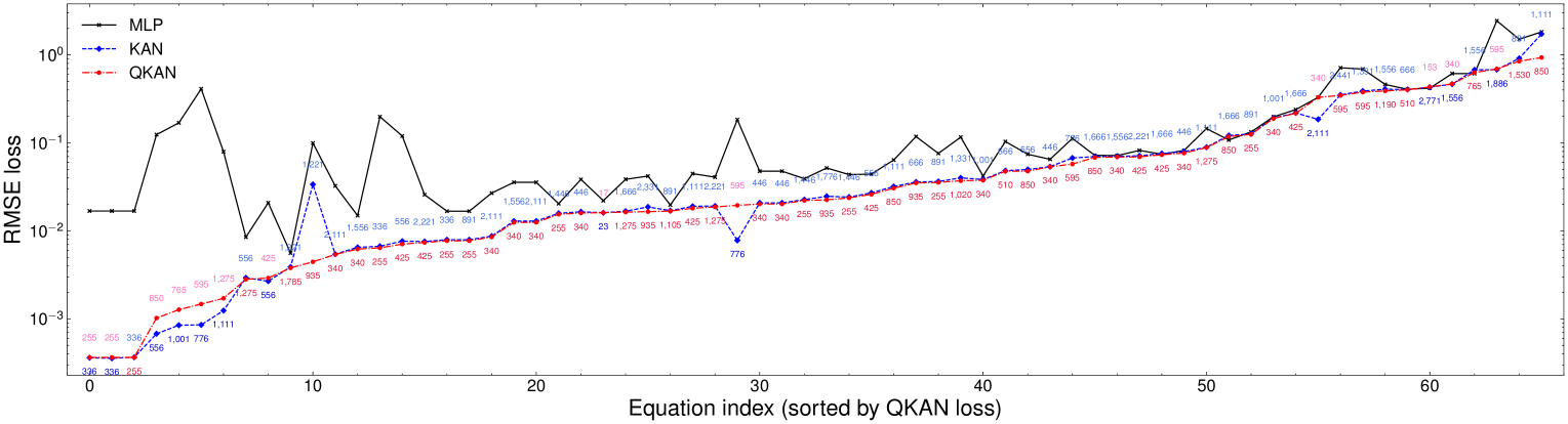
Figure 5: Empirical noisy function fitting. For each equation, we report the average test RMSE of each model with the best depths of hidden layers. The colored annotations in blue indicate the number of parameters for KANs and in red for QKANs, whence the lower the better. The results show that QKANs can achieve the best test RMSE over 80% of the equations, and with much fewer parameters than KANs in most of the cases.

In addition to the summary presented in Figure˜5, we provide the complete set in LABEL:tab:com_reg. This table includes the full list of 66 equations used in the regression benchmark, which were not explicitly shown in the main text. For each equation, we report the RMSE loss and the number of trainable parameters for both QKAN and classical KAN models. These results further illustrate that QKANs can achieve comparable or superior approximation accuracy while maintaining significantly fewer parameters.

Table 5: Detailed regression results corresponding to Figure˜5. This table presents a comparison between QKAN and classical KAN across 66 symbolic regression expressions. For each expression, we report the root mean square error (RMSE) loss and the total number of trainable parameters. Bold values highlight the better-performing model in each row (lower RMSE). The results demonstrate that QKAN consistently achieves comparable or superior approximation accuracy with significantly fewer parameters, validating the expressive efficiency of DARUAN.

Equation		QKAN		KAN
Idx	Expression	RMSE Loss	# Params	RMSE Loss	# Params
1	$\hbar\omega$	$3.652\times 10^{-04}$	255	$\mathbf{3.619\times 10^{-04}}$	$\mathbf{336}$
2	$N_{n}\mu$	$3.652\times 10^{-04}$	255	$\mathbf{3.568\times 10^{-04}}$	336
3	$E_{f}q_{2}$	$\mathbf{3.652\times 10^{-04}}$	255	$3.662\times 10^{-04}$	336
4	$0.5m\left(u^{2}+v^{2}+w^{2}\right)$	$1.023\times 10^{-03}$	850	$\mathbf{6.779\times 10^{-04}}$	556
5	$Fr\sin{(\theta)}$	$1.274\times 10^{-03}$	765	$\mathbf{8.490\times 10^{-04}}$	1,001
6	$x_{1}y_{1}+x_{2}y_{2}+x_{3}y_{3}$	$1.476\times 10^{-03}$	595	$\mathbf{8.556\times 10^{-04}}$	776
7	$mrv\sin{\theta}$	$1.715\times 10^{-03}$	1,275	$\mathbf{1.244\times 10^{-03}}$	1,111
8	$0.25mx^{2}\left(\omega^{2}+\omega_{0}^{2}\right)$	$\mathbf{2.818\times 10^{-03}}$	1,275	$2.933\times 10^{-03}$	556
9	${p_{d}\cos{\theta}}/{4\pi\epsilon r^{2}}$	$2.915\times 10^{-03}$	425	$\mathbf{2.683\times 10^{-03}}$	556
10	${\hbar\omega^{3}}/{\pi^{2}c^{2}\left(\exp\left({\hbar\omega}/{Tk_{b}}\right)-1\right)}$	$\mathbf{3.800\times 10^{-03}}$	1,785	$3.898\times 10^{-03}$	1,221
11	$q\left(Bv\sin{\theta}+E_{f}\right)$	$\mathbf{4.455\times 10^{-03}}$	935	$3.377\times 10^{-02}$	1,221
12	$2U\left(1-\cos{\left(dk\right)}\right)$	$\mathbf{5.404\times 10^{-03}}$	340	$5.442\times 10^{-03}$	2,111
13	${qrv}/{2}$	$\mathbf{6.219\times 10^{-03}}$	340	$6.503\times 10^{-03}$	1,556
14	$\left(x+y\right)\sin{\left(\exp({2y})\right)}$	$\mathbf{6.419\times 10^{-03}}$	255	$6.693\times 10^{-03}$	336
15	${3p_{d}\sin{\theta}\cos{\theta}}/{4\pi\epsilon r^{3}}$	$\mathbf{7.082\times 10^{-03}}$	425	$7.648\times 10^{-03}$	556
16	${E_{f}\alpha\epsilon n}/({-{\alpha n}/{3}+1})$	$\mathbf{7.388\times 10^{-03}}$	425	$7.572\times 10^{-03}$	2,221
17	$0.5k_{s}x^{2}$	$\mathbf{7.729\times 10^{-03}}$	255	$7.942\times 10^{-03}$	336
18	$0.5E_{f}^{2}\epsilon$	$\mathbf{7.729\times 10^{-03}}$	255	$7.937\times 10^{-03}$	891
19	$E_{f}^{2}c\epsilon$	$\mathbf{8.531\times 10^{-03}}$	340	$8.722\times 10^{-03}$	2,111
20	$gmz$	$\mathbf{1.249\times 10^{-02}}$	340	$1.293\times 10^{-02}$	1,556
21	$Tk_{b}\mu$	$\mathbf{1.249\times 10^{-02}}$	340	$1.294\times 10^{-02}$	2,111
22	$E_{f}^{2}\epsilon$	$\mathbf{1.546\times 10^{-02}}$	255	$1.586\times 10^{-02}$	1,446
23	${I_{0}\sin^{2}{\left({n\theta}/{2}\right)}}/{\sin^{2}{\left({\theta}/{2}\right)}}$	$\mathbf{1.598\times 10^{-02}}$	340	$1.650\times 10^{-02}$	446
24	${\sqrt{2}\exp({-{\theta^{2}}/{2}})}/{2\sqrt{\pi}}$	$1.611\times 10^{-02}$	17	$\mathbf{1.611\times 10^{-02}}$	23
25	${4I_{0}\sin^{2}{\left({\alpha}/{2}\right)}\sin^{2}{\left({N\delta}/{2}\right)}}/{\alpha^{2}\sin^{2}{\left({\delta}/{2}\right)}}$	$\mathbf{1.637\times 10^{-02}}$	1,275	$1.676\times 10^{-02}$	1,666
26	${n_{0}}/\left({\exp({{B\mu}/{Tk_{b}}})+\exp({-{B\mu}/{Tk_{b}}})}\right)$	$\mathbf{1.655\times 10^{-02}}$	935	$1.872\times 10^{-02}$	2,331
27	${Y}/({2\sigma+2})$	$\mathbf{1.681\times 10^{-02}}$	1,105	$1.700\times 10^{-02}$	891
28	${l}/{2\pi c^{2}\epsilon r}$	$\mathbf{1.810\times 10^{-02}}$	425	$1.903\times 10^{-02}$	1,111
29	${\hbar\omega}/({\exp({{\hbar\omega}/{Tk_{b}}})-1})$	$\mathbf{1.872\times 10^{-02}}$	1,275	$1.920\times 10^{-02}$	2,221
30	$(-{H^{2}c^{2}\cdot\left(1-2\alpha\right)+{c^{4}k_{f}}/{a_{f}^{2}}})/{8\pi G}$	$1.952\times 10^{-02}$	595	$\mathbf{7.809\times 10^{-03}}$	776
31	$-B\mu_{M}\cos{\theta}$	$\mathbf{2.023\times 10^{-02}}$	340	$2.084\times 10^{-02}$	446
32	$-E_{f}p_{d}\cos{\theta}$	$\mathbf{2.023\times 10^{-02}}$	340	$2.082\times 10^{-02}$	446
33	$\operatorname{asin}{\left(n\sin{\theta_{2}}\right)}$	$\mathbf{2.219\times 10^{-02}}$	255	$2.270\times 10^{-02}$	1,446
34	$\mu n\tanh{\left({B\mu}/{Tk_{b}}\right)}$	$\mathbf{2.254\times 10^{-02}}$	935	$2.473\times 10^{-02}$	1,776
35	$\hbar n$	$\mathbf{2.372\times 10^{-02}}$	255	$2.427\times 10^{-02}$	1,446
36	${d\left(1-\alpha^{2}\right)}/({\alpha\cos{\left(\theta_{1}-\theta_{2}\right)}+1})$	$\mathbf{2.603\times 10^{-02}}$	425	$2.709\times 10^{-02}$	556
37	${E}/{({E\left(1-\cos{\theta}\right)}/{c^{2}m}+1)}$	$\mathbf{3.062\times 10^{-02}}$	850	$3.198\times 10^{-02}$	1,111
38	$Tk_{b}n\log{\left({V_{2}}/{V_{1}}\right)}$	$\mathbf{3.509\times 10^{-02}}$	935	$3.597\times 10^{-02}$	666
39	$1.5Vp_{F}$	$\mathbf{3.558\times 10^{-02}}$	255	$3.645\times 10^{-02}$	891
40	$n_{0}\exp({-{gmx}/{Tk_{b}}})$	$\mathbf{3.716\times 10^{-02}}$	1,020	$4.005\times 10^{-02}$	1,331
41	$B\mu\left(\chi+1\right)$	$\mathbf{3.761\times 10^{-02}}$	340	$3.845\times 10^{-02}$	1,001
42	${3\left(H^{2}+{c^{2}k_{f}}/{a_{f}^{2}}\right)}/{8\pi G}$	$\mathbf{4.767\times 10^{-02}}$	510	$4.834\times 10^{-02}$	666
43	$\mu\sqrt{B_{x}^{2}+B_{y}^{2}+B_{z}^{2}}$	$\mathbf{4.778\times 10^{-02}}$	850	$4.992\times 10^{-02}$	556
44	${1}/({{n}/{d_{2}}+{1}/{d_{1}}})$	$\mathbf{5.355\times 10^{-02}}$	340	$5.372\times 10^{-02}$	446
45	$V_{e}q+\sqrt{c^{4}m^{2}+c^{2}\left(-Aq+p\right)^{2}}$	$\mathbf{5.753\times 10^{-02}}$	595	$6.745\times 10^{-02}$	776
46	${1}/({\exp({{\hbar\omega}/{Tk_{b}}})-1})$	$\mathbf{6.836\times 10^{-02}}$	850	$6.983\times 10^{-02}$	1,666
47	$\beta\left(\alpha\cos{\theta}+1\right)$	$\mathbf{6.930\times 10^{-02}}$	340	$7.042\times 10^{-02}$	1,556
48	$x_{1}\left(\alpha\cos^{2}{\left(\omega t\right)}+\cos{\left(\omega t\right)}\right)$	$\mathbf{6.938\times 10^{-02}}$	425	$7.132\times 10^{-02}$	2,221
49	$({m_{1}r_{1}+m_{2}r_{2}})/({m_{1}+m_{2}})$	$\mathbf{7.342\times 10^{-02}}$	425	$7.578\times 10^{-02}$	1,666
50	$\sqrt{{\gamma p}/{\rho}}$	$\mathbf{7.662\times 10^{-02}}$	340	$7.965\times 10^{-02}$	446
51	$\sqrt{x_{1}^{2}-2x_{1}x_{2}\cos{\left(\theta_{1}-\theta_{2}\right)}+x_{2}^{2}}$	$\mathbf{8.846\times 10^{-02}}$	1,275	$8.931\times 10^{-02}$	1,111
52	$\sqrt{\left(-x_{1}+x_{2}\right)^{2}+\left(-y_{1}+y_{2}\right)^{2}}$	$\mathbf{1.181\times 10^{-01}}$	850	$1.215\times 10^{-01}$	1,666
53	${\alpha n}/({-{\alpha n}/{3}+1})+1$	$\mathbf{1.252\times 10^{-01}}$	255	$1.265\times 10^{-01}$	891
54	$I_{1}+I_{2}+2\sqrt{I_{1}I_{2}}\cos{\left(\delta\right)}$	$\mathbf{1.896\times 10^{-01}}$	340	$1.920\times 10^{-01}$	1,001
55	${k_{b}v}/{A\left(\gamma-1\right)}$	$\mathbf{2.172\times 10^{-01}}$	425	$2.192\times 10^{-01}$	1,666
56	$\sin^{2}{\left({Et}/{\hbar}\right)}$	$3.291\times 10^{-01}$	340	$\mathbf{1.853\times 10^{-01}}$	2,111
57	${3p_{d}z\sqrt{x^{2}+y^{2}}}/{4\pi\epsilon r^{5}}$	$\mathbf{3.467\times 10^{-01}}$	595	$3.517\times 10^{-01}$	2,441
58	${k_{G}m\left(\sqrt{{2EL^{2}}/{k_{G}^{2}m}+1}\cos{\left(\theta_{1}-\theta_{2}\right)}+1\right)}/{L^{2}}$	$\mathbf{3.777\times 10^{-01}}$	595	$3.887\times 10^{-01}$	1,331
59	${\sqrt{2}\exp({-{\left(\theta-\theta_{1}\right)^{2}}/{2\sigma^{2}}})}/{2\sqrt{\pi}\sqrt{\sigma^{2}}}$	$\mathbf{3.895\times 10^{-01}}$	1,190	$4.078\times 10^{-01}$	1,556
60	$\sqrt{{8\pi G\rho}/{3}-{c^{2}k_{f}}/{a_{f}^{2}}}$	$\mathbf{4.017\times 10^{-01}}$	510	$4.050\times 10^{-01}$	666
61	${Gm_{1}m_{2}}/({\left(-x_{1}+x_{2}\right)^{2}+\left(-y_{1}+y_{2}\right)^{2}+\left(-z_{1}+z_{2}\right)^{2}})$	$4.331\times 10^{-01}$	153	$\mathbf{4.295\times 10^{-01}}$	2,771
62	${Vp_{F}}/({\gamma-1})$	$4.681\times 10^{-01}$	340	$\mathbf{4.655\times 10^{-01}}$	1,556
63	${hq}/{4\pi m}$	$\mathbf{6.304\times 10^{-01}}$	765	$6.766\times 10^{-01}$	1,556
64	$({m^{2}\omega^{2}x^{2}\left({\alpha y}/{x}+1\right)+p^{2}})/{2m}$	$6.937\times 10^{-01}$	595	$\mathbf{6.810\times 10^{-01}}$	1,886
65	${\sqrt{2}\exp({-{\theta^{2}}/{2\sigma^{2}}})}/{2\sqrt{\pi}\sqrt{\sigma^{2}}}$	$\mathbf{8.487\times 10^{-01}}$	1,530	$9.130\times 10^{-01}$	891
66	${q}/{\sqrt{d^{2}-2dr\cos{\alpha}+r^{2}}}$	$\mathbf{9.339\times 10^{-01}}$	850	$1.731\times 10^{+00}$	1,111

B.2 Visualization of QKAN Activations on Noisy Function Regression

To further analyze the expressive power and interpretability of QKANs, we visualize the learned activation functions from selected regression tasks involving noisy symbolic expressions. This follows a similar methodology to KANs, where each activation function is a learnable one-dimensional function, enabling insight into the internal structure of the model.

Figure˜6 presents the per-node activation functions learned by QKANs that achieved the lowest RMSE for representative equations drawn from the benchmark in Table˜1. These visualizations demonstrate that QKANs are capable of learning smooth, structured nonlinearities even in the presence of input noise, highlighting their robustness and alignment with symbolic structure.

Figure 6: Visualization of learned QKAN activations for heuristic noisy regression equations. This figure illustrates the per-node activation functions learned by QKANs, similar to the interpretability offered by KANs. We display the QKAN models that achieved the lowest RMSE for a subset of representative symbolic regression equations, as listed in Table˜1. The transparency of each node is proportional to output range divided by input range; darker therefore denote stronger connections. Each sub-panel corresponds to a distinct equation, demonstrating that QKANs can learn smooth and structured nonlinear transformations despite the presence of noise.

Appendix C Experimental Details

C.1 Software Implementation

To enable efficient numerical simulation of QKANs on CUDA-enabled devices [NVIDIA et al., 2020], we build our implementation using PyTorch [Ansel et al., 2024], extending its tensor operations with custom routines for quantum state evolution.

The quantum state is represented as a complex-valued tensor with shape $(B,N,M,2)$, where $B$ denotes the batch size, $N$ is the number of post-nodes, $M$ is the number of pre-nodes, and the final dimension encodes the amplitudes of the 2-level quantum system (i.e., a single qubit).

Quantum gates are encoded as complex tensors with shape $(N,M,2,2)$, where the last two dimensions represent the $2\times 2$ matrix structure of a single-qubit unitary gate, and the first two dimensions index the interaction between input and output nodes.

We adopt the Pauli-$Z$ operator as the observable for measurement. The data encoding blocks and trainable unitaries in the data re-uploading ansatz are implemented as parameterized single-qubit rotation gates.

To initialize the quantum state, a Hadamard gate is applied to place the qubit into an equal superposition of basis states, which empirically improves the stability and convergence of training.

C.2 Software and System Information

For full reproducibility, Table˜6 summarizes the software versions, dependencies, and hardware system specifications used in our experiments.

Table 6: Software and System Information.

Software	Version
matplotlib	3.6.2
wandb	0.16.6
tqdm	4.66.2
h5py	3.11.0
numpy	1.24.4
scikit_learn	1.1.3
setuptools	65.5.0
sympy	1.11.1
pandas	2.0.3
requests	2.31.0
transformers	4.40.1
PennyLane	0.37.0
PennyLane_Lightning	0.37.0
torch	2.4.0
torchaudio	2.4.0
torchvision	2.4.0
pykan	0.0.5
RTX 4090 Personal Computer
Parameter	Value
Python version	3.11.5
Python compiler	GCC 11.2.0
Python build	main, Sep 11 2023 13:54:46
OS	Linux
CPUs	1
CPUs Memory (GB)	64
GPUs	1 (NVIDIA GeForce RTX 4090)
GPUs Memory (GB)	24
Mon Sep 16 08:47:24 2024 UTC
Tesla V100S Single Node Cluster
Parameter	Value
Python version	3.11.11
Python compiler	GCC 11.2.0
Python build	main, Dec 11 2024, 16:28:39
OS	Linux
GPUs	4 (Tesla V100S-PCIE-32GB)
GPUs Memory (GB)	128
Fri Mar 29 18:32:15 2025 UTC
NVIDIA H100 GPUs & NVIDIA H200 GPUs Cluster
Parameter	Value
Python version	3.11.13
Python compiler	GCC 11.2.0
Python build	main, Jun 5 2025, 13:12:00
OS	Linux
Scheduling System	Slurm Workload Manager
GPUs on a H100 node	8 (NVIDIA H100 PCIe)
GPUs Memory (GB) on a H100 node	640
GPUs on a H200 node	8 (NVIDIA H200 PCIe)
GPUs Memory (GB) on a H200 node	1128
Cross-node Interconnector	8 InfiniBand NDR 400G network ports
Wed Jul 2 23:10:24 2025 UTC

References

- Abd Elaziz et al. [2024] Mohamed Abd Elaziz, Ibrahim Ahmed Fares, and Ahmad O. Aseeri. Ckan: Convolutional kolmogorov–arnold networks model for intrusion detection in iot environment. IEEE Access, 12:134837–134851, 2024. doi: 10.1109/ACCESS.2024.3462297.
- Aghaei [2024] Alireza Afzal Aghaei. fKAN: Fractional kolmogorov-arnold networks with trainable jacobi basis functions, 2024. URL https://arxiv.org/abs/2406.07456.
- Agostinelli et al. [2015] Forest Agostinelli, Matthew Hoffman, Peter Sadowski, and Pierre Baldi. Learning activation functions to improve deep neural networks, 2015. URL https://arxiv.org/abs/1412.6830.
- Ansel et al. [2024] Jason Ansel et al. Pytorch 2: Faster machine learning through dynamic python bytecode transformation and graph compilation. In Proceedings of the 29th ACM International Conference on Architectural Support for Programming Languages and Operating Systems, Volume 2, ASPLOS ’24, page 929–947, New York, NY, USA, 2024. Association for Computing Machinery. ISBN 9798400703850. doi: 10.1145/3620665.3640366.
- Apicella et al. [2021] Andrea Apicella, Francesco Donnarumma, Francesco Isgrò, and Roberto Prevete. A survey on modern trainable activation functions. Neural Networks, 138:14–32, June 2021. ISSN 0893-6080. doi: 10.1016/j.neunet.2021.01.026. URL http://dx.doi.org/10.1016/j.neunet.2021.01.026.
- Biamonte et al. [2017] Jacob Biamonte, Peter Wittek, Nicola Pancotti, Patrick Rebentrost, Nathan Wiebe, and Seth Lloyd. Quantum machine learning. Nature, 549(7671):195–202, September 2017. ISSN 1476-4687. doi: 10.1038/nature23474. URL http://dx.doi.org/10.1038/nature23474.
- Bozorgasl and Chen [2024] Zavareh Bozorgasl and Hao Chen. Wav-kan: Wavelet kolmogorov-arnold networks, 2024. URL https://arxiv.org/abs/2405.12832.
- Brown et al. [2020] Tom B. Brown et al. Language models are few-shot learners, 2020. URL https://arxiv.org/abs/2005.14165.
- Chen and Liang [2025] Samuel Yen-Chi Chen and Zhiding Liang. Introduction to quantum machine learning and quantum architecture search, 2025. URL https://arxiv.org/abs/2504.16131.
- Chen and Yoo [2021] Samuel Yen-Chi Chen and Shinjae Yoo. Federated quantum machine learning. Entropy, 23(4), 2021. ISSN 1099-4300. doi: 10.3390/e23040460. URL https://www.mdpi.com/1099-4300/23/4/460.
- Chen et al. [2020] Samuel Yen-Chi Chen, Chao-Han Huck Yang, Jun Qi, Pin-Yu Chen, Xiaoli Ma, and Hsi-Sheng Goan. Variational quantum circuits for deep reinforcement learning. IEEE Access, 8:141007–141024, 2020. doi: 10.1109/ACCESS.2020.3010470.
- Ciliberto et al. [2018] Carlo Ciliberto et al. Quantum machine learning: a classical perspective. Proceedings of the Royal Society A: Mathematical, Physical and Engineering Sciences, 474(2209):20170551, January 2018. ISSN 1471-2946. doi: 10.1098/rspa.2017.0551. URL http://dx.doi.org/10.1098/rspa.2017.0551.
- Dao et al. [2022] Tri Dao, Daniel Y. Fu, Stefano Ermon, Atri Rudra, and Christopher Ré. Flashattention: Fast and memory-efficient exact attention with io-awareness, 2022. URL https://arxiv.org/abs/2205.14135.
- Deng [2012] Li Deng. The mnist database of handwritten digit images for machine learning research [best of the web]. IEEE Signal Processing Magazine, 29(6):141–142, 2012. doi: 10.1109/MSP.2012.2211477.
- Devadas and T [2025] Raghavendra M Devadas and Sowmya T. Quantum machine learning: A comprehensive review of integrating ai with quantum computing for computational advancements. MethodsX, 14:103318, 2025. ISSN 2215-0161. doi: https://doi.org/10.1016/j.mex.2025.103318. URL https://www.sciencedirect.com/science/article/pii/S2215016125001645.
- Douzette [2017] Andre Sevaldsen Douzette. B-splines in machine learning. Master’s thesis, 2017.
- Dunjko et al. [2016] Vedran Dunjko, Jacob M. Taylor, and Hans J. Briegel. Quantum-enhanced machine learning. Phys. Rev. Lett., 117:130501, Sep 2016. doi: 10.1103/PhysRevLett.117.130501. URL https://link.aps.org/doi/10.1103/PhysRevLett.117.130501.
- Farhi and Neven [2018] Edward Farhi and Hartmut Neven. Classification with quantum neural networks on near term processors, 2018. URL https://arxiv.org/abs/1802.06002.
- Ganesh [2024] Aditya Nalgunda Ganesh. Kan-gpt: The pytorch implementation of generative pre-trained transformers (gpts) using kolmogorov-arnold networks (kans) for language modeling, May 2024. URL https://github.com/AdityaNG/kan-gpt/. Release 1.0.0, 9th May 2024.
- Genet and Inzirillo [2024] Remi Genet and Hugo Inzirillo. Tkan: Temporal kolmogorov-arnold networks, 2024. URL https://arxiv.org/abs/2405.07344.
- Girosi and Poggio [1989] Federico Girosi and Tomaso Poggio. Representation properties of networks: Kolmogorov’s theorem is irrelevant. Neural Comput., 1(4):465–469, December 1989. ISSN 0899-7667. doi: 10.1162/neco.1989.1.4.465. URL https://doi.org/10.1162/neco.1989.1.4.465.
- Harrow et al. [2009] Aram W. Harrow, Avinatan Hassidim, and Seth Lloyd. Quantum algorithm for linear systems of equations. Physical Review Letters, 103(15), October 2009. ISSN 1079-7114. doi: 10.1103/physrevlett.103.150502. URL http://dx.doi.org/10.1103/PhysRevLett.103.150502.
- He et al. [2015] Kaiming He, Xiangyu Zhang, Shaoqing Ren, and Jian Sun. Delving deep into rectifiers: Surpassing human-level performance on imagenet classification. In 2015 IEEE International Conference on Computer Vision (ICCV), pages 1026–1034, 2015. doi: 10.1109/ICCV.2015.123.
- Howard et al. [2024] Amanda A. Howard, Bruno Jacob, Sarah H. Murphy, Alexander Heinlein, and Panos Stinis. Finite basis kolmogorov-arnold networks: domain decomposition for data-driven and physics-informed problems, 2024. URL https://arxiv.org/abs/2406.19662.
- Inajetovic et al. [2023] Matteo Antonio Inajetovic, Filippo Orazi, Antonio Macaluso, Stefano Lodi, and Claudio Sartori. Enabling non-linear quantum operations through variational quantum splines. In Jiří Mikyška, Clélia de Mulatier, Maciej Paszynski, Valeria V. Krzhizhanovskaya, Jack J. Dongarra, and Peter M.A. Sloot, editors, Computational Science – ICCS 2023, pages 177–192, Cham, 2023. Springer Nature Switzerland. ISBN 978-3-031-36030-5.
- Jerbi et al. [2023] Sofiene Jerbi, Lukas J. Fiderer, Hendrik Poulsen Nautrup, Jonas M. Kübler, Hans J. Briegel, and Vedran Dunjko. Quantum machine learning beyond kernel methods. Nature Communications, 14(1), January 2023. ISSN 2041-1723. doi: 10.1038/s41467-023-36159-y. URL http://dx.doi.org/10.1038/s41467-023-36159-y.
- Jiang [2025] Jiun-Cheng Jiang. Quantum-inspired kolmogorov-arnold network, 2025. URL https://github.com/Jim137/qkan.
- Karpathy [2022] Andrej Karpathy. nanogpt, 2022. URL https://github.com/karpathy/nanoGPT.
- Kingma and Ba [2014] Diederik P. Kingma and Jimmy Ba. Adam: A method for stochastic optimization. CoRR, abs/1412.6980, 2014. URL https://api.semanticscholar.org/CorpusID:6628106.
- Kolmogorov [1957] Andrei Nikolaevich Kolmogorov. On the representation of continuous functions of many variables by superposition of continuous functions of one variable and addition. In Doklady Akademii Nauk, volume 114, pages 953–956. Russian Academy of Sciences, 1957.
- Krizhevsky and Hinton [2009] Alex Krizhevsky and Geoffrey Hinton. Learning multiple layers of features from tiny images. Technical Report 0, University of Toronto, Toronto, Ontario, 2009. URL https://www.cs.toronto.edu/~kriz/learning-features-2009-TR.pdf.
- Li et al. [2024a] Chenxin Li et al. U-kan makes strong backbone for medical image segmentation and generation, 2024a. URL https://arxiv.org/abs/2406.02918.
- Li et al. [2024b] Shaozhi Li, M Sabbir Salek, Yao Wang, and Mashrur Chowdhury. Quantum-inspired activation functions and quantum chebyshev-polynomial network, 2024b. URL https://arxiv.org/abs/2404.05901.
- Li [2024] Ziyao Li. Kolmogorov-arnold networks are radial basis function networks, 2024.
- Liu et al. [2024a] Chen-Yu Liu et al. Quantum-train: Rethinking hybrid quantum-classical machine learning in the model compression perspective, 2024a. URL https://arxiv.org/abs/2405.11304.
- Liu and Nocedal [1989] Dong C. Liu and Jorge Nocedal. On the limited memory bfgs method for large scale optimization. Mathematical Programming, 45:503–528, 1989. URL https://api.semanticscholar.org/CorpusID:5681609.
- Liu et al. [2024b] Ziming Liu, Pingchuan Ma, Yixuan Wang, Wojciech Matusik, and Max Tegmark. Kan 2.0: Kolmogorov-arnold networks meet science, 2024b. URL https://arxiv.org/abs/2408.10205.
- Liu et al. [2024c] Ziming Liu et al. Kan: Kolmogorov-arnold networks. arXiv preprint arXiv:2404.19756, 2024c. URL https://arxiv.org/abs/2404.19756.
- Loshchilov and Hutter [2017] Ilya Loshchilov and Frank Hutter. Decoupled weight decay regularization. In International Conference on Learning Representations, 2017. URL https://api.semanticscholar.org/CorpusID:53592270.
- Mari et al. [2020] Andrea Mari, Thomas R. Bromley, Josh Izaac, Maria Schuld, and Nathan Killoran. Transfer learning in hybrid classical-quantum neural networks. Quantum, 4:340, October 2020. ISSN 2521-327X. doi: 10.22331/q-2020-10-09-340. URL http://dx.doi.org/10.22331/q-2020-10-09-340.
- McClean et al. [2018] Jarrod R McClean, Sergio Boixo, Vadim N Smelyanskiy, Ryan Babbush, and Hartmut Neven. Barren plateaus in quantum neural network training landscapes. Nature communications, 9(1):4812, 2018.
- Meyer et al. [2023] Johannes Jakob Meyer et al. Exploiting symmetry in variational quantum machine learning. PRX Quantum, 4(1), March 2023. ISSN 2691-3399. doi: 10.1103/prxquantum.4.010328. URL http://dx.doi.org/10.1103/PRXQuantum.4.010328.
- Mitarai et al. [2018] K. Mitarai, M. Negoro, M. Kitagawa, and K. Fujii. Quantum circuit learning. Physical Review A, 98(3), September 2018. ISSN 2469-9934. doi: 10.1103/physreva.98.032309. URL http://dx.doi.org/10.1103/PhysRevA.98.032309.
- Molina et al. [2019] Alejandro Molina, Patrick Schramowski, and Kristian Kersting. Padé activation units: End-to-end learning of flexible activation functions in deep networks. In International Conference on Learning Representations, 2019.
- NVIDIA et al. [2020] NVIDIA, Péter Vingelmann, and Frank H.P. Fitzek. Cuda, release: 10.2.89, 2020. URL https://developer.nvidia.com/cuda-toolkit.
- Phillipson [2020] Frank Phillipson. Quantum machine learning: Benefits and practical examples. In QANSWER, pages 51–56, 2020.
- Poggio et al. [2020] Tomaso Poggio, Andrzej Banburski, and Qianli Liao. Theoretical issues in deep networks. Proceedings of the National Academy of Sciences, 117(48):30039–30045, 2020.
- Preskill [2018] John Preskill. Quantum Computing in the NISQ era and beyond. Quantum, 2:79, August 2018. ISSN 2521-327X. doi: 10.22331/q-2018-08-06-79. URL https://doi.org/10.22331/q-2018-08-06-79.
- Pérez-Salinas et al. [2020] Adrián Pérez-Salinas, Alba Cervera-Lierta, Elies Gil-Fuster, and José I. Latorre. Data re-uploading for a universal quantum classifier. Quantum, 4:226, February 2020. ISSN 2521-327X. doi: 10.22331/q-2020-02-06-226. URL http://dx.doi.org/10.22331/q-2020-02-06-226.
- Radford et al. [2019] Alec Radford, Jeff Wu, and Jong Wook Kim. gpt-2-output-dataset. https://github.com/openai/gpt-2-output-dataset, 2019.
- Ramachandran et al. [2017] Prajit Ramachandran, Barret Zoph, and Quoc V. Le. Searching for activation functions, 2017. URL https://arxiv.org/abs/1710.05941.
- Rower et al. [2024] David A. Rower et al. Suppressing counter-rotating errors for fast single-qubit gates with fluxonium. PRX Quantum, 5:040342, Dec 2024. doi: 10.1103/PRXQuantum.5.040342. URL https://link.aps.org/doi/10.1103/PRXQuantum.5.040342.
- Scardapane et al. [2019] Simone Scardapane, Steven Van Vaerenbergh, Simone Totaro, and Aurelio Uncini. Kafnets: Kernel-based non-parametric activation functions for neural networks. Neural Networks, 110:19–32, 2019. ISSN 0893-6080. doi: https://doi.org/10.1016/j.neunet.2018.11.002. URL https://www.sciencedirect.com/science/article/pii/S0893608018303174.
- Schuld and Killoran [2019] Maria Schuld and Nathan Killoran. Quantum machine learning in feature hilbert spaces. Phys. Rev. Lett., 122:040504, Feb 2019. doi: 10.1103/PhysRevLett.122.040504. URL https://link.aps.org/doi/10.1103/PhysRevLett.122.040504.
- Schuld et al. [2021] Maria Schuld, Ryan Sweke, and Johannes Jakob Meyer. Effect of data encoding on the expressive power of variational quantum-machine-learning models. Physical Review A, 103(3), March 2021. ISSN 2469-9934. doi: 10.1103/physreva.103.032430. URL http://dx.doi.org/10.1103/PhysRevA.103.032430.
- Seydi [2024a] Seyd Teymoor Seydi. Exploring the potential of polynomial basis functions in kolmogorov-arnold networks: A comparative study of different groups of polynomials, 2024a. URL https://arxiv.org/abs/2406.02583.
- Seydi [2024b] Seyd Teymoor Seydi. Unveiling the power of wavelets: A wavelet-based kolmogorov-arnold network for hyperspectral image classification, 2024b. URL https://arxiv.org/abs/2406.07869.
- Shuai et al. [2024] Xian Shuai, Yiding Wang, Yimeng Wu, Xin Jiang, and Xiaozhe Ren. Scaling law for language models training considering batch size, 2024. URL https://arxiv.org/abs/2412.01505.
- Singh et al. [2024] Akhil Pratap Singh et al. Experimental demonstration of a high-fidelity virtual two-qubit gate. Physical Review Research, 6(1), March 2024. ISSN 2643-1564. doi: 10.1103/physrevresearch.6.013235. URL http://dx.doi.org/10.1103/PhysRevResearch.6.013235.
- Smith et al. [2025] M. C. Smith, A. D. Leu, K. Miyanishi, M. F. Gely, and D. M. Lucas. Single-qubit gates with errors at the level. Phys. Rev. Lett., 134:230601, Jun 2025. doi: 10.1103/42w2-6ccy. URL https://link.aps.org/doi/10.1103/42w2-6ccy.
- SS et al. [2024] Sidharth SS, Keerthana AR, Gokul R, and Anas KP. Chebyshev polynomial-based kolmogorov-arnold networks: An efficient architecture for nonlinear function approximation, 2024. URL https://arxiv.org/abs/2405.07200.
- Ta [2024] Hoang-Thang Ta. Bsrbf-kan: A combination of b-splines and radial basis functions in kolmogorov-arnold networks, 2024. URL https://arxiv.org/abs/2406.11173.
- Udrescu and Tegmark [2020] Silviu-Marian Udrescu and Max Tegmark. AI Feynman: a Physics-Inspired Method for Symbolic Regression. Sci. Adv., 6(16):eaay2631, 2020. doi: 10.1126/sciadv.aay2631.
- Udrescu et al. [2020] Silviu-Marian Udrescu, Andrew Tan, Jiahai Feng, Orisvaldo Neto, Tailin Wu, and Max Tegmark. Ai feynman 2.0: pareto-optimal symbolic regression exploiting graph modularity. In Proceedings of the 34th International Conference on Neural Information Processing Systems, NIPS ’20, Red Hook, NY, USA, 2020. Curran Associates Inc. ISBN 9781713829546.
- Vaca-Rubio et al. [2024] Cristian J. Vaca-Rubio, Luis Blanco, Roberto Pereira, and Màrius Caus. Kolmogorov-arnold networks (kans) for time series analysis, 2024. URL https://arxiv.org/abs/2405.08790.
- Wach et al. [2023] Noah L. Wach, Manuel S. Rudolph, Fred Jendrzejewski, and Sebastian Schmitt. Data re-uploading with a single qudit. Quantum Machine Intelligence, 5(2), August 2023. ISSN 2524-4914. doi: 10.1007/s42484-023-00125-0. URL http://dx.doi.org/10.1007/s42484-023-00125-0.
- Wakaura et al. [2025a] Hikaru Wakaura, Rahmat Mulyawan, and Andriyan B. Suksmono. Adaptive variational quantum kolmogorov-arnold network, 2025a. URL https://arxiv.org/abs/2503.21336.
- Wakaura et al. [2025b] Hikaru Wakaura, Rahmat Mulyawan, and Andriyan B. Suksmono. Enhanced variational quantum kolmogorov-arnold network, 2025b. URL https://arxiv.org/abs/2503.22604.
- Werner et al. [2025] Yannick Werner, Akash Malemath, Mengxi Liu, Vitor Fortes Rey, Nikolaos Palaiodimopoulos, Paul Lukowicz, and Maximilian Kiefer-Emmanouilidis. Qukan: A quantum circuit born machine approach to quantum kolmogorov arnold networks, 2025. URL https://arxiv.org/abs/2506.22340.
- Xie et al. [2024] Xinke Xie, Yang Lu, Chong-Yung Chi, Wei Chen, Bo Ai, and Dusit Niyato. Kansformer for scalable beamforming, 2024. URL https://arxiv.org/abs/2410.20690.
- Xingyi Yang [2025] Xinchao Wang Xingyi Yang. Kolmogorov-arnold transformer. In The Thirteenth International Conference on Learning Representations, 2025. URL https://openreview.net/forum?id=BCeock53nt.
- Xu et al. [2024a] Jinfeng Xu et al. Fourierkan-gcf: Fourier kolmogorov-arnold network – an effective and efficient feature transformation for graph collaborative filtering, 2024a. URL https://arxiv.org/abs/2406.01034.
- Xu et al. [2024b] Kunpeng Xu, Lifei Chen, and Shengrui Wang. Kolmogorov-arnold networks for time series: Bridging predictive power and interpretability, 2024b. URL https://arxiv.org/abs/2406.02496.
- Yu et al. [2024a] Runpeng Yu, Weihao Yu, and Xinchao Wang. Kan or mlp: A fairer comparison, 2024a. URL https://arxiv.org/abs/2407.16674.
- Yu et al. [2022] Zhan Yu, Hongshun Yao, Mujin Li, and Xin Wang. Power and limitations of single-qubit native quantum neural networks, 2022. URL https://arxiv.org/abs/2205.07848.
- Yu et al. [2024b] Zhan Yu et al. Non-asymptotic approximation error bounds of parameterized quantum circuits, 2024b. URL https://arxiv.org/abs/2310.07528.
- Zhao et al. [2024] Jiaming Zhao, Wenbo Qiao, Peng Zhang, and Hui Gao. Quantum implicit neural representations. arXiv preprint arXiv:2406.03873, 2024.