Schrödinger-invariance in the voter model

Malte Henkel^a,b and Stoimen Stoimenov^c

^aLaboratoire de Physique et Chimie Théoriques (CNRS UMR 7019),

Université de Lorraine Nancy, B.P. 70239, F – 54506 Vandœuvre lès Nancy Cedex, France

^bCentro de Física Teórica e Computacional, Universidade de Lisboa,

Campo Grande, P – 1749-016 Lisboa, Portugal

^c Institute of Nuclear Research and Nuclear Energy, Bulgarian Academy of Sciences,

72 Tsarigradsko chaussee, Blvd., BG – 1784 Sofia, Bulgaria

Exact single-time and two-time correlations and the two-time response function are found for the order-parameter in the voter model with nearest-neighbour interactions. Their explicit dynamical scaling functions are shown to be continuous functions of the space dimension $d>0$. Their form reproduces the predictions of non-equilibrium representations of the Schrödinger algebra for models with dynamical exponent $\mathpzc{z}=2$ and with the dominant noise-source coming from the heat bath. Hence the ageing in the voter model is a paradigm for relaxations in non-equilibrium critical dynamics, without detailed balance, and with the upper critical dimension $d^{*}=2$.

1 Introduction: physical ageing in the voter model

The understanding of the collective behaviour of many-body systems out of equilibrium continues to pose many challenges [84, 21, 35, 5, 6, 88]. Since exact solutions are only exceptionally available and numerical simulations may require large resources in computer facilities, the use of symmetries may provide additional and complementary insight. A remarkable and often-studied case is physical ageing [82], formally characterised by its three defining properties [47]: (I) slow relaxational dynamics, (II) absence of time-translation-invariance and (III) dynamical scaling. In classical systems ageing is usually realised by preparing a system in a totally disordered initial state before quenching it instantaneously either onto a critical point $T=T_{c}>0$ or else into the disordered phase with temperature $T<T_{c}$. When $T=T_{c}$, one speaks of non-equilibrium critical dynamics [38] whereas for $T<T_{c}$, one is dealing with phase-ordering kinetics [10]. At $T=T_{c}$, the dynamics is characterised by critical-point fluctuations, whereas for $T<T_{c}$ there is a competition of at least two distinct, but equivalent, equilibrium states and the dynamics is driven by the interface tension between them [10]. In either case, the system becomes spatially non-homogeneous and decomposes microscopically into clusters of a time-dependent and growing linear size $\ell=\ell(t)$. We shall admit that this growth is algebraic at late times, viz. $\ell(t)\sim t^{1/\mathpzc{z}}$, which defines the dynamical exponent $\mathpzc{z}$. A convenient characterisation uses the time-space-dependent order-parameter $\phi(t,\boldsymbol{r})$ – in pure magnetic systems identified as the coarse-grained local magnetisation. For a totally disordered initial state we can admit that on average the initial order-parameter vanishes, such that for all times $\left\langle\phi(t,\boldsymbol{r})\right\rangle=\left\langle\phi(0,\boldsymbol{r})\right\rangle=0$. The study of such systems is centred on analysing the single-time and two-time correlation function $C$ and the two-time response function $R$, defined as

$$C(t,s;{r})=\bigl\langle\phi(t,\boldsymbol{r})\phi(s,\boldsymbol{0})\bigr\rangle\;\;,\;\;R(t,s;{r})=\left.\frac{\delta\bigl\langle\phi(t,\boldsymbol{r})\bigr\rangle}{\delta h(s,\boldsymbol{0})}\right|_{h=0}=\bigl\langle\phi(t,\boldsymbol{r})\widetilde{\phi}(s,\boldsymbol{0})\bigr\rangle$$ (1.1)

where the average is both over initial states as well as over thermal histories. We shall always admit the habitual spatial translation- and rotation-invariances, such that $\boldsymbol{r}\mapsto r=|\boldsymbol{r}|$, for notational simplicity. In (1.1) we anticipate from Janssen-de Dominicis theory [22, 55] that $R$ can be formally rewritten as a correlator with the so-called response scaling operator $\widetilde{\phi}(t,\boldsymbol{r})$, to be often-used in this work. Setting $t=s$ in (1.1) gives the single-time correlator $C(s;r):=C(s,s;r)$. Setting $r=0$ in (1.1) produces the auto-correlator $C(t,s):=C(t,s;{0})$ and the auto-response $R(t,s):=R(t,s;{0})$. Throughout, we shall assume model-A-type dynamics without any macroscopic conservation law.

In this work, we shall study the physical ageing of the so-called voter-model [62, 63, 86, 59], in $d>0$ spatial dimensions which we shall consider as a continuous variable. Precise definitions will be given in section 2. Before that, we shall begin with a qualitative overview, immediately in the continuum limit, first on the generic ageing behaviour and second on the model-specific properties. As the first example we consider the single-time correlator, for dimensions $d<2$ in figure 1 and for dimensions $d>2$ in figure 2. Figure 1ab displays $C(s;r)$ for two examples where the dimension $d<2$, for several values of the time $s$. In both cases, we see that with increasing $s$, the decay of the correlator slows down such that the dynamics becomes more slow when the system has grown more old, which is the slow-dynamics property (I). Property (II) follows since for different values of $s$ one obtains distinct curves. Finally, the curves collapse onto a single one when replotted over against $r/\sqrt{s}$ and these are shown together in figure 1c, where for comparison we also added the curve corresponding to $d=1$. This demonstrates property (III). The same exercise is carried out in figure 2 for two examples with $d>2$. As before, we can verify the first two defining properties (I) and (II) in figure 2ab. Property (III) is the data collapse with respect to the variable $r/\sqrt{s\,}$ when the single-time correlator is rescaled by $s^{d/2-1}$. In figure 2c we display the shape of the scaling function, for three different values of $d$.

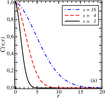
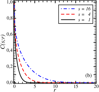
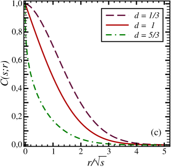
Figure 1: Physical ageing in the single-time correlator of the voter model for $d<2$ dimensions. Panel (a) shows $C(s;r)$ for $d=1/3$ and $s=[1,4,16]$. Panel (b) shows $C(s;r)$ for $d=5/3$ and the same three values of $s$. Panel (c) shows the associated scaling function of $C(s;r)=F_{C}\bigl(1;r/\sqrt{s\,}\,\bigr)$ for the dimensions $d=[1/3,1,5/3]$ from top to bottom.

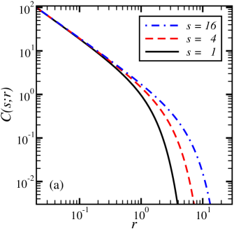
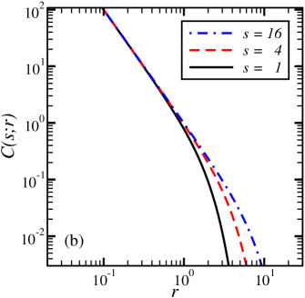
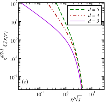
Figure 2: Physical ageing in the single-time correlator of the voter model for $d>2$ dimensions. Panel (a) shows $C(s;r)$ for $d=3$ and $s=[1,4,16]$. Panel (b) shows $C(s;r)$ for $d=4$ and the same values of $s$. Panel (c) shows the scaling function $s^{d/2-1}C(s;r)=F_{C}\bigl(1;r/\sqrt{s\,}\,\bigr)$ for the dimensions $d=[3,4,5]$ from bottom to top.

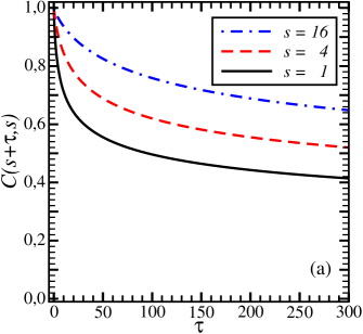
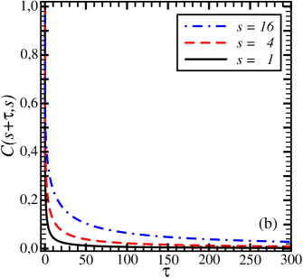
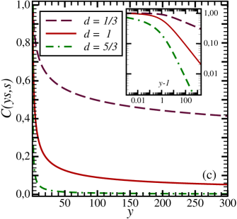
Figure 3: Physical ageing in the two-time auto-correlator $C(t,s)$ of the voter model for $d<2$ dimensions. Panel (a) shows $C(s+\tau,s)$ for $d=1/3$ and three values of $s$. Panel (b) shows $C(s+\tau,s)$ for $d=5/3$, the same values of $s$ and at the same scale. Panel (c) shows the associated scaling function $C(ys,s)=f_{C}(y)$ for the dimensions $d=[1/3,1,5/3]$. The inset displays $f_{C}(y)$ over against $y-1$, in order to show the power-law decay for $y\gg 1$.

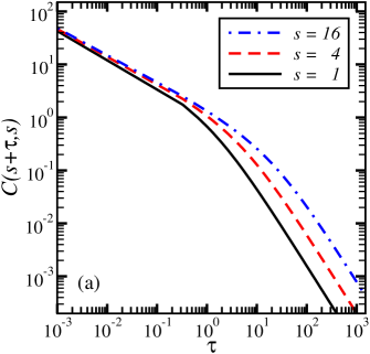
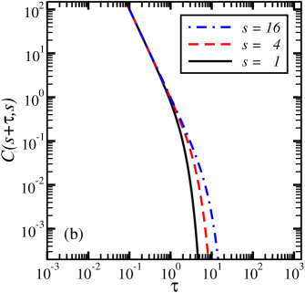
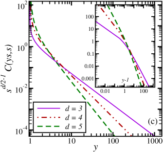
Figure 4: Physical ageing in the two-time correlator of the voter model for $d>2$ dimensions. Panel (a) shows $C(s+\tau,s)$ for $d=3$ and three values of $s$. Panel (b) shows $C(s+\tau,s)$ for $d=4$, the same values of $s$, at the same scale. Panel (c) shows the scaling function $s^{d/2-1}C(ys,s)=f_{C}(y)$ for the dimensions $d=[3,4,5]$. The inset displays $f_{C}(y)$ over against $y-1$, and shows the cross-over between two power-laws for $y\gg 1$ and $y-1\ll 1$, respectively.

Analogously, we now consider the ageing behaviour as it manifests itself in the two-time auto-correlator $C(t,s)$ which is shown in figure 3 for $d<2$ and figure 4 for $d>2$. Following the analogy with the single-time correlator, we show in figure 3ab the auto-correlator, over against the time difference $\tau=t-s$, for two examples of dimensions $d<2$, for three values of the waiting time $s$. As before, we can verify the three defining properties of ageing: (I) with increasing values of $s$, the auto-correlator decays more slowly, (II) for different values of $s$ one has distinct curves such that $C(t,s)=C(s+\tau,s)$ does not only depend on $\tau$ and (III) these curves collapse onto a single one when replotted over against $y=t/s$, see figure 3c, where again we also added the curve with $d=1$ for later comparison. The same exercise is carried out in figure 4 for dimensions $d>2$, with analogous results. The properties (I) and (II) are checked in figure 4ab and the shape of the scaling function is shown in figure 4c, for the same values of $d$ as above for the single-time correlator, which demonstrates property (III). Overall, we can conclude that the voter model in all dimensions $d>0$ does satisfy the generic properties of physical ageing. Formally, this can be cast into the scaling forms

$$C(t,s;{r})=s^{-b}F_{C}\left(\frac{t}{s};\frac{\bigl|\boldsymbol{r}\bigr|}{s^{1/\mathpzc{z}}}\right)\;\;,\;\;R(t,s;{r})=s^{-1-a}F_{R}\left(\frac{t}{s};\frac{\bigl|\boldsymbol{r}\bigr|}{s^{1/\mathpzc{z}}}\right)$$ (1.2a)

with the ageing exponents $$b,a T=T_{c} a=b=(d-2+\eta)/\mathpzc{z} \eta T<T_{c} b=0 a=\frac{1}{2} \mathpzc{z}=2 y\gg 1$$. For non-equilibrium critical dynamics at in pure magnetic systems, one generically expects that [38, 12, 47, 84], where is a standard equilibrium critical exponent; whereas for phase-ordering kinetics at in magnetic systems one expects but and , at least in pure systems with short-ranged interactions [10, 45, 47]. In addition, one usually finds asymptotically for

$$f_{C}(y)=F_{C}(y;0)\sim y^{-\lambda_{C}/\mathpzc{z}}\;\;,\;\;f_{R}(y)=F_{R}(y;0)\sim y^{-\lambda_{R}/\mathpzc{z}}$$ (1.2b)

where $$\lambda_{C} \lambda_{R} d$$ is the auto-correlation exponent [54] and is the auto-response exponent [71]. This algebraic form is bourne out in figures 3c and 4c in the voter model for the auto-correlator, for all values of the dimension . In almost all models, provided only that the initial correlations are spatially short-ranged, one also expects that [9, 10, 38, 72]

$$\lambda=\lambda_{C}=\lambda_{R}$$ (1.2c)

The scaling functions $F_{C,R}\bigl(y,rs^{-1/\mathpzc{z}}\bigr)$ in (1.2a) are expected universal, by which it is meant that their form should be independent of microscopic ‘details’, such as the lattice structure, the precise form of the interactions, or of temperature upon a quench into $T<T_{c}$. On the other hand, one expects them to be $d$-dependent.

Having established that the generic set-up of physical ageing is applicable to the nearest-neighbour voter model, we now consider its more specific aspects which involve the form of the scaling functions. In all cases, one has the dynamical exponent $\mathpzc{z}=2$. For the single-time correlator $C(s;r)$, comparison of their shapes in figures 1c and 2c, respectively, shows that they are very different. Although in all dimensions, the decay for large values of the scaling variable $r/\sqrt{s\,}$ is more fast than any power-law, for small values of this scaling variable there is a saturation at $C(s;0)=1$ for $d<2$ but a power-law behaviour in $r/\sqrt{s\,}\ll 1$ whenever $d>2$. In figure 1c we see that when $d<2$ the $r$-dependent approach towards $C(s;0)=1$ depends clearly on the value of $d$. When $d>2$, the respective exponent is seen to be $d$-dependent from figure 2c. We also notice that while for $d<2$ the single-time correlator scales directly, for $d>2$ the single-time correlator must be rescaled according to $s^{d/2-1}C(s;r)$ in order to achieve the scaling collapse and that the scaling functions decrease with $d$ for $d<2$ while they increase with $d$ for $d>2$ (in our normalisation, see section 2). The reason behind such different behaviour calls for an explanation. Similarly, we compare the shapes of the two-time auto-correlator $C(t,s)$ in figures 3c and 4c. Again for $d<2$ and $d>2$, respectively, we find very different shapes and possibly distinct dependencies on $d$. Although for large values of the scaling variable $y=t/s$ the decay is algebraic for all dimensions $d>0$ (which also shows that the relaxation times are formally infinite such that the ageing system will never reach a stationary state) and in agreement with the expected (1.2b), we also observe here a saturation at $C(s,s)=1$ for $d<2$ with a $d$-dependent approach as a function of $y-1$ (inset of figure 3c) while there is a power-law behaviour in $y-1\ll 1$ for $d>2$, with a $d$-dependent exponent (inset of figure 4c). Also, we observe that for $d<2$, the auto-correlator $C(ys,s)$ is $s$-independent and directly scales whereas for $d>2$, a data collapse is seen for the rescaling auto-correlator $s^{d/2-1}C(ys,s)$. An explanation for this must be sought as well. This will come from the exact expressions for all these scaling functions which we shall calculate explicitly.

Finally, we shall use the exactly solvable voter model to test generic ideas on the form of these scaling functions, which is our main motivation to undertake this work. Evidently, all observations for which we provided examples in the figures will be confirmed from the exact results, for all $d>0$. From the details of its definition (see section 2) it will become apparent that the voter model is actually at a critical point between two non-critical phases [58]. Then the scaling form of its observables will be determined by the fluctuations coming from the thermal bath but will be independent of the fluctuations of the initial state (in the renormalisation-group sense, the latter ones are irrelevant and will contribute at most to corrections to the leading behaviour, onto which we shall focus exclusively). Since the dynamical exponent $\mathpzc{z}=2$, it is tempting to generalise the dynamical scaling symmetry, by definition present in any physically ageing system, and demonstrated to hold for the voter model in figures 1c,2c,3c and 4c, to a larger symmetry. The natural candidate for this is the Schrödinger group, which is known to be a dynamical symmetry of the free diffusion equation from the work of Jacobi and Lie in the middle of the 19^th century, see [27] for a historical review. The first applications to dynamics in statistical physics date at least back to [43]. More recently, it has been understood how to adapt the (equilibrium) predictions of Schrödinger-invariance, by a change of the Lie algebra representation, to the far-from-equilibrium context of physical ageing [48, 50]. Especially for systems with a dynamical exponent $\mathpzc{z}=2$ and which undergo non-equilibrium critical dynamics for which the fluctuations of the heat bath are relevant, very recently we derived the generic form of the scaling function $F_{C}\bigl(1;r/\sqrt{s\,}\,\bigr)$ of the single-time correlator and also for $f_{C}(y)$ of the two-time auto-correlator (modulo a technical hypothesis which will turn out to be valid in the voter model) [51], see section 3. By construction, the results of a dynamical symmetry, if applicable, are universal. In addition, the dynamical Schrödinger symmetry reduces the problem of finding the form of a scaling function (which in principle requires to determine infinitely many parameters) to the determination of a finite (and small) set of parameters and whose values are furthermore related between different observables. We shall use the voter model, in any dimension $d>0$, to test (and eventually confirm) these predictions. It is suggestive to consider non-integer values of $d$ as akin to study the voter model on a fractal [83, 4, 40] although it is known that a fractal geometry is characterised by more than one fractal dimension [75, 70, 61, 32]. We shall also include an explicit treatment when the voter model is at its upper critical dimension $d=d^{*}=2$. We shall see that a different non-equilibrium representation of the Schrödinger Lie algebra must be used. Altogether, this work provides a new kind of evidence that the $d$-dimensional voter model falls into the class of non-equilibrium critical dynamics.

This work is organised as follows. In section 2 we present the exact solution of the voter model, with nearest-neighbour interactions, and derive explicit expressions for the correlators $C(s;r)$ and $C(t,s)$ as well as for the response function $R(t,s;r)$ whose scaling functions depend continuously on $d>0$. In section 3 we recall the necessary background on non-equilibrium field-theory, on Schrödinger-invariance at equilibrium and on how to map the results onto non-equilibrium observables. In section 4 we compare the exact results from section 2 with the field-theoretic predictions of non-equilibrium Schrödinger-invariance and thereby confirm that the non-equilibrium voter model is indeed Schrödinger-invariant for all dimensions $d>0$. We conclude in section 5.

2 The voter model

The much-studied voter model can be formulated as a classical spin model, defined in terms of spin variables $\sigma_{\boldsymbol{n}}=\pm 1$ attached to the sites $\boldsymbol{n}\in\Lambda\subset\mathbb{Z}^{d}$ of a hyper-cubic lattice in $d$ dimensions. A spin configuration is denoted as $\{\sigma\}=\bigl(\sigma_{1},\ldots,\sigma_{\cal N}\bigr)$, where ${\cal N}=|\Lambda|$ is the total number of sites. That configuration arises with the probability $P\bigl(\{\sigma\},t\bigr)$. The dynamics is described in terms of a master equation

$$\partial_{t}P\bigl(\{\sigma\},t)=\sum_{\{\sigma^{\prime}\}}\left[w\bigl(\{\sigma^{\prime}\}\to\{\sigma\}\bigr)P\bigl(\{\sigma^{\prime}\},t)-w\bigl(\{\sigma\}\to\{\sigma^{\prime}\}\bigr)P\bigl(\{\sigma\},t)\right]$$ (2.1)

In the voter model, transitions between configurations occur via single spin flips. If the spin to be flipped is at site $\boldsymbol{n}$, the transition rates of the voter model are [62, 63, 86, 59]

$$w\bigl(\{\sigma\}\to\{\sigma^{\prime}\}\bigr)~~\mapsto~~w_{\boldsymbol{n}}\bigl(\{\sigma\}\bigr)=\frac{1}{2}\left(1-\frac{1}{2d}\sigma_{\boldsymbol{n}}\sum_{\boldsymbol{m}(\boldsymbol{n})}\sigma_{\boldsymbol{m}}\right)$$ (2.2)

where $\boldsymbol{m}(\boldsymbol{n})$ are the nearest-neighbour sites with respect to the site $\boldsymbol{n}\in\Lambda$. The model appears to have been first introduced in the 1960s in studies of genetic correlations before receiving profound interest from probability theory, see [62, 19] and refs. therein. It has numerous applications: for example it is often construed (possibly with generalisations) as a simple model for opinion-forming [14, 76, 29] or is used in the modelling of network dynamics [87, 13, 24, 8]. In a physical context, it was re-discovered either as a simple model of a non-equilibrium spin system subject to two distinct baths, each creating its proper dynamics at its own temperature [25, 26], or in surface catalytic reactions [58, 68] or as a prototype of critical-point ageing in models with several absorbing states [23]. It is one of the very few models of interacting spins which is analytically solvable in any number of dimensions, for any kind of interactions [58, 30, 31, 87]. With the widely studied Glauber-Ising model [36] it shares the invariance under a total spin-reversal $\sigma_{\boldsymbol{n}}\mapsto-\sigma_{\boldsymbol{n}}$ for all $\boldsymbol{n}\in\Lambda$. In contrast to the Glauber-Ising model, the voter model does not satisfy the detailed-balance condition [62, 63, 86, 59, 39] such that its stationary states cannot be at thermal equilibrium. Rather, the voter model has two absorbing states, namely $\sigma_{\boldsymbol{n}}=1$ for all $\boldsymbol{n}\in\Lambda$ (or $\sigma_{\boldsymbol{n}}=-1$ for all $\boldsymbol{n}$) into which the system may enter but it cannot leave. Still, although “the voter model belongs to a different universality class, some of [its] features …have a clear counterpart in ferromagnetic models” [19]. The solubility of the voter model has been used to carry out a detailed set of studies on its ageing behaviour in the presence of long-range interactions with distant-dependent interaction rates $w(r)\sim r^{-\alpha}$, first numerically for $d=1$ [77] and recently in a long series of analytical studies [15, 16, 17, 18, 19, 20] in $d=1,2,3$ dimensions. While for $\alpha>2+d$, the late-time behaviour is the same as for the nearest neighbour rates (2.2), a very rich and new behaviour is found for smaller values of $\alpha$. Since in these new long-ranged regimes, the dynamical exponent $\mathpzc{z}<2$ if it exists at all [15, 16, 19], we cannot use those results in our planned comparison with Schrödinger-invariance and therefore shall restrict ourselves to the nearest-neighbour rates (2.2). However, we shall consider the continuous dependence of the scaling functions on the dimension $d>0$ which allows to take advantage of the voter model as a paradigmatic case of ageing without detailed balance. New insight beyond what would be accessible when restricting to $d=1,2,3$ will be obtained.

Before we begin our analysis of correlators and responses, we add two more comments. First, consider the average order parameter $S_{\boldsymbol{n}}(t)=\bigl\langle\sigma_{\boldsymbol{n}}\bigr\rangle(t)$. From the master equation, equations of motion for $S_{\boldsymbol{n}}$ are readily derived, using $\partial_{t}\langle\sigma_{\boldsymbol{n}}\rangle=-2\langle\sigma_{\boldsymbol{n}}w_{\boldsymbol{n}}\rangle$, and lead to [58] $S_{\boldsymbol{n}}(t)=e^{-dt}\sum_{\boldsymbol{m}}S_{\boldsymbol{n}-\boldsymbol{m}}(0)I_{n_{1}-m_{1}}(t)\cdots I_{n_{d}-m_{d}}(t)$. Since for a fully disordered initial state $S_{\boldsymbol{n}}(t)=S_{\boldsymbol{n}}(0)=0$ for all times $t>0$, at least on average the two stationary states are never reached in a spatially infinite system. Second, the density $n_{\rm r}(t)$ of reactive $`+-^{\prime}$-interfaces, expressed in terms of a nearest-neighbour correlator, is evaluated for large times as [30, 68, 14]

$$n_{\rm r}(t)=\frac{1}{2}\biggl(1-\bigl\langle\sigma_{\boldsymbol{n}}\sigma_{\boldsymbol{n}+\boldsymbol{1}}\bigr\rangle\biggr)\sim\left\{\begin{array}[]{ll}t^{-(2-d)/2}&\mbox{\rm~~;~ if $d<2$}\\ 1/\ln t&\mbox{\rm~~;~ if $d=2$}\\ \mathfrak{a}-\mathfrak{b}t^{-d/2}&\mbox{\rm~~;~ if $d>2$}\end{array}\right.$$ (2.3)

where $\mathfrak{a},\mathfrak{b}$ are constants. This points to an important difference between the $d<2$ and $d>2$ cases: it is generally said that for $d\leq 2$ the voter model undergoes coarsening since $n_{\rm r}(t)\to 0$ and for $d>2$, there are infinitely many stationary states since $n_{\rm r}(t)$ remains finite [62, 63].

2.1 Single-time correlator

In what follows, the spatial continuum limit will be taken throughout. Then the single-time spin-spin correlator $C_{\boldsymbol{n}}(t)=\bigl\langle\sigma_{\boldsymbol{n}}\sigma_{\boldsymbol{0}}\bigr\rangle(t)$ will become $C(t;\boldsymbol{r})=\bigl\langle\phi(t,\boldsymbol{r})\phi(t,\boldsymbol{0})\bigr\rangle$ in terms of a coarse-grained order-parameter $\phi(t,\boldsymbol{r})$. Inserting the rate (2.2) into the master equation leads after rescaling to the equation of motion for the single-time correlator

$$\partial_{t}C(t;r)=\Delta_{\boldsymbol{r}}C(t;r)=\left(\partial_{r}^{2}+(d-1)\frac{1}{r}\partial_{r}\right)C(t;r)$$ (2.4)

where $\Delta_{\boldsymbol{r}}$ is the spatial laplacian and we also used that in the continuum limit, spatial translation- and rotation-invariance are restored. Then the correlator merely depends on the absolute value $r=|\boldsymbol{r}|$. Eq. (2.4) will be the basis of all subsequent calculations. To solve this equation, we use the scaling ansatz [58, 86, 19]

$$C(t;r)=t^{-b}F_{C}\bigl(\mathfrak{u}\bigr)\;\;,\;\;\mathfrak{u}=rt^{-1/2}$$ (2.5)

where $b$ will be identified later on with one of the ageing exponents. Clearly, $\mathpzc{z}=2$. Eq. (2.5) implies the double scaling limit $t\to\infty$, $r\to\infty$ such that $\mathfrak{u}$ is kept fixed. From now on $d$ can be treated as a continuous parameter. It follows that the scaling function obeys the differential equation

$$F_{C}^{\prime\prime}(\mathfrak{u})+(d-1)\frac{1}{\mathfrak{u}}F_{C}^{\prime}(\mathfrak{u})+\frac{1}{2}\mathfrak{u}F_{C}^{\prime}(\mathfrak{u})+bF_{C}(\mathfrak{u})=0$$ (2.6)

with the general solution [57]

$$F_{C}(\mathfrak{u})=\mathscr{C}_{1}\,e^{-\mathfrak{u}^{2}/4}\,M\left(\frac{d}{2}-b,\frac{d}{2};\frac{\mathfrak{u}^{2}}{4}\right)+\mathscr{C}_{2}\,e^{-\mathfrak{u}^{2}/4}\,U\left(\frac{d}{2}-b,\frac{d}{2};\frac{\mathfrak{u}^{2}}{4}\right)$$ (2.7)

where $M,U$ are the confluent Kummer hypergeometric functions [1] and $\mathscr{C}_{1,2}$ are constants.

Next, we find the value of the exponent $b$ from the stationary solution which obeys [86]

$$\Delta_{\boldsymbol{r}}C(\infty;r)=0~~\Longrightarrow~~\left(\partial_{\mathfrak{u}}^{2}+(d-1)\frac{1}{\mathfrak{u}}\partial_{\mathfrak{u}}\right)f(\mathfrak{u})=0$$ (2.8)

with the solution $f(\mathfrak{u})=f_{0}+f_{1}\mathfrak{u}^{2-d}$ where $f_{0,1}$ are constants. Because of the definition (2.5) of $\mathfrak{u}$, the stationary limit $t\to\infty$ corresponds to $\mathfrak{u}\ll 1$. In that limit, we have for $d<2$ that $f(\mathfrak{u})\to f_{0}$ saturates and for $d>2$ that $f(\mathfrak{u})\to f_{1}\mathfrak{u}^{2-d}$ is reminiscent of an equilibrium critical correlator $C_{\rm eq}(r)\sim r^{-(d-2+\eta)}$. Combining this with the scaling from (2.5) allows us to conclude

$$b=\left\{\begin{array}[]{ll}0&\mbox{\rm~~;~ if $d<2$}\\ (d-2)/2&\mbox{\rm~~;~ if $d>2$}\end{array}\right.$$ (2.9)

The case $d=2$ is treated separately since the ansatz (2.5) will no longer work, see section 2.4.

1. Inserting the result (2.9) into (2.7) gives for $d<2$

$$C(t;r)=\mathscr{C}_{1}\,e^{-r^{2}/4t}\,M\left(\frac{d}{2},\frac{d}{2};\frac{r^{2}}{4t}\right)+\mathscr{C}_{2}\,e^{-r^{2}/4t}\,U\left(\frac{d}{2},\frac{d}{2};\frac{r^{2}}{4t}\right)=\mathscr{C}_{1}+\mathscr{C}_{2}\,e^{-r^{2}/4t}\,U\left(\frac{d}{2},\frac{d}{2};\frac{r^{2}}{4t}\right)$$ (2.10)

Since $b=0$, the boundary conditions are that $C(t;r)\to 0$ as $r\to\infty$ more fast than any power and that $C(t;r)\to 1$ as $r\to 0$. Using the known asymptotics of the Kummer/Tricomi function $U$ [1], we have for $r\to\infty$ that $C(t;r)\simeq\mathscr{C}_{1}+\mathscr{C}_{2}\,e^{-r^{2}/4t}\,\bigl(\frac{r^{2}}{4t}\bigr)^{-d/2}$ which can only decay for $\mathscr{C}_{1}=0$. The second boundary condition leads via [1, (13.1.6)] to $\mathscr{C}_{2}\,\Gamma\bigl(1-\frac{d}{2}\bigr)\stackrel{{\scriptstyle!}}{{=}}1$, so that the final solution reads

$$C(t;r)=\frac{1}{\Gamma\bigl(1-\frac{d}{2}\bigr)}\,e^{-r^{2}/4t}\,U\left(\frac{d}{2},\frac{d}{2};\frac{r^{2}}{4t}\right)=\frac{\Gamma\bigl(1-\frac{d}{2},\frac{r^{2}}{4t}\bigr)}{\Gamma\bigl(1-\frac{d}{2}\bigr)}\;\;;\;\;d<2$$ (2.11a)

but can also be expressed in terms of an incomplete Gamma function [1, (13.6.28)]. It does agree with the generic scaling expectation (1.2a).

If $d=1$, the voter model becomes identical to the Glauber-Ising chain and we reproduce the known result $C^{(1D)}(t;r)=\frac{1}{\sqrt{\pi\,}}e^{-r^{2}/4t}\,U\bigl(\frac{1}{2},\frac{1}{2};\frac{r^{2}}{4t}\bigr)={\rm erfc\,}\bigl(\frac{r}{2\sqrt{t\,}}\bigr)$ [11, 37, 15, 49] as expected.

In ferromagnets which undergo phase-ordering kinetics, the single-time correlator satisfies to well-known Porod’s law [73, 10]. In the $d=1$ special case, equivalent to the Glauber-Ising chain, we have the initially linear decay $C^{(1D)}(t;r)\simeq 1-\frac{1}{\sqrt{\pi\,}}\frac{|r|}{\sqrt{t\,}}+\ldots$ and Porod’s law holds true. More generally in the voter model, a small-distance expansion of (2.11a) gives

$$C(t;r) = \frac{\Gamma\bigl(\frac{d}{2}-1\bigr)}{\Gamma\bigl(\frac{d}{2}\bigr)\Gamma\bigl(1-\frac{d}{2}\bigr)}\left(\frac{\boldsymbol{r}^{2}}{4t}\right)^{1-d/2}e^{-\boldsymbol{r}^{2}/4t}{}_{1}F_{1}\left(1;2-\frac{d}{2};\frac{\boldsymbol{r}^{2}}{4t}\right)+e^{-\boldsymbol{r}^{2}/4t}{}_{1}F_{1}\left(\frac{d}{2};\frac{d}{2};\frac{\boldsymbol{r}^{2}}{4t}\right)$$ (2.12)

$$\simeq 1-\frac{2^{d-2}}{\Gamma\bigl(2-\frac{d}{2}\bigr)}\left(\frac{\boldsymbol{r}^{2}}{t}\right)^{1-d/2}+\ldots\;\;;\;\;d<2$$

which does not lead to a linear decay of the single-time correlator for small $r$ and Porod’s law does not hold for $d\neq 1$, see also figure 1c. Since for small $d$, the initial decay is more slow than linear and for dimensions close to $d=2$, it is much more fast, by continuity we would have expected to find an intermediate dimension, where the decay happens to be linear, as it occurs indeed for $d=1$. In addition, we can also consider the structure factor

$$\widehat{S}(t;\boldsymbol{q}) := \int_{\mathbb{R}^{d}}\!{\rm d}\boldsymbol{r}\>e^{-{\rm i}\boldsymbol{q}\cdot\boldsymbol{r}}\,C(t;r)\>=\>\frac{1}{\Gamma\bigl(1-\frac{d}{2}\bigr)}\int_{\mathbb{R}^{d}}\!{\rm d}\boldsymbol{r}\>e^{-{\rm i}\boldsymbol{q}\cdot\boldsymbol{r}-\frac{1}{4}\boldsymbol{r}^{2}/t}\,U\left(\frac{d}{2},\frac{d}{2};\frac{\boldsymbol{r}^{2}}{4t}\right)$$ (2.13)

$$= \frac{\bigl(4\pi\bigr)^{d/2}\Gamma\bigl(\frac{d}{2}+1\bigr)}{\Gamma\bigl(1-\frac{d}{2}\bigr)\Gamma\bigl(\frac{d}{2}\bigr)}t^{d/2}\,{}_{1}F_{1}\left(1;\frac{d}{2}+1;-t\boldsymbol{q}^{2}\right)\;\;;\;\;d<2$$

which was evaluated via the integral representation [1, (13.2.5)] for $U$. This certainly has the expected scaling form $\widehat{S}(t;\boldsymbol{q})=\widehat{S}_{0}q^{-d}f\bigl(\boldsymbol{q}^{2}t\bigr)$. But asymptotically for $q=|\boldsymbol{q}|\to\infty$, we have with [1, (13.5.1)] that $\widehat{S}(t;\boldsymbol{q})\sim t^{d/2-1}q^{-2}$. This agrees with the expected Porod form $\sim q^{-d-1}$ [73, 10] only for $d=1$. We conclude that unsurprisingly, the dynamics of the voter model is in general different from the phase-ordering kinetics of a ferromagnet at $T<T_{c}$, since generically, it does not satisfy detailed balance.

2. For $d>2$, we have from (2.9) that $b=(d-2)/2$ and read off from (2.7)

$$C(t;r)=\mathscr{C}_{1}\,t^{-(d-2)/2}\,e^{-r^{2}/4t}\,M\left(1,\frac{d}{2};\frac{r^{2}}{4t}\right)+\mathscr{C}_{2}\,t^{-(d-2)/2}\,e^{-r^{2}/4t}\,U\left(1,\frac{d}{2};\frac{r^{2}}{4t}\right)$$ (2.14)

For $r\to\infty$, with [1, (13.1.4)] and [1, (13.1.8)] this gives

$$C(t;r)\simeq\mathscr{C}_{1}\,\Gamma\left(\frac{d}{2}\right)\,r^{2-d}+\mathscr{C}_{2}\,t^{-d/2}\,r^{-2}\,e^{-r^{2}/4t}$$ (2.15)

which should vanish more fast with $r$ than any power. This is only possible for $\mathscr{C}_{1}=0$. On the other hand, for $r\to 0$ we find [1, (13.5.8)] $C(t;r)\simeq\mathscr{C}_{2}\,2^{d-2}\Gamma\bigl(\frac{d}{2}-1\bigr)\,r^{2-d}$. Here, since we have taken the continuum limit from the outset, it is no longer possible to achieve a saturation. One might arbitrarily prescribe a fixed value $C(t;\mathfrak{a})$ at some ‘small’ distance $\mathfrak{a}$, i.e. [58, 30, 59, 85, 19], but we rather prefer to accept that in the continuum limit, the stationary scaling solution $C(\infty;r)\sim r^{-(d-2)}$ does not saturate when $r\to 0$. Then at most we can impose an equality of amplitudes, of the kind $\mathscr{C}_{2}\,\Gamma\bigl(\frac{d}{2}-1\bigr)2^{d-2}\stackrel{{\scriptstyle!}}{{=}}\mathfrak{C}_{0}$ such that our final solution is

$$C(t;r)=\frac{\mathfrak{C}_{0}}{2^{d-2}\Gamma\bigl(\frac{d}{2}-1\bigr)}t^{-d/2+1}\,e^{-r^{2}/4t}\,U\left(1,\frac{d}{2};\frac{r^{2}}{4t}\right)=\mathfrak{C}_{0}\,r^{2-d}\frac{\Gamma\bigl(\frac{d}{2}-1,\frac{r^{2}}{4t}\bigr)}{\Gamma\bigl(\frac{d}{2}-1\bigr)}\;\;;\;\;d>2$$ (2.11b)

and $\mathfrak{C}_{0}$ is the amplitude of the stationary correlator for $d>2$. The two equations (2.11) together give the single-time correlator for all dimensions $d\neq 2$ and will serve as input for the calculations of the other observables. They prove analytically what we showed by example in figures 1c and 2c. This suggests that for $d<2$ the voter model still shares some properties with systems undergoing phase-ordering kinetics, whereas for $d>2$ it behaves more like a system undergoing non-equilibrium critical dynamics.

If $d=3$, we have with [1, (13.1.7)]

$$C^{(3D)}(t;r) = \frac{\mathfrak{C}_{0}}{2\Gamma\bigl(\frac{1}{2}\bigr)}t^{-1/2}\,e^{-r^{2}/4t}\,U\left(1,\frac{3}{2};\frac{r^{2}}{4t}\right)$$ (2.16)

$$= \frac{\mathfrak{C}_{0}}{2\sqrt{\pi\,}}t^{-1/2}\,e^{-r^{2}/4t}\left(\frac{r^{2}}{4t}\right)^{-1/2}\,U\left(\frac{1}{2},\frac{1}{2};\frac{r^{2}}{4t}\right)\>=\>\mathfrak{C}_{0}\,r^{-1}{\rm erfc\,}\left(\frac{r}{2\sqrt{t\,}}\right)$$

which via [1, (13.6.39)] does reproduce the known result [19, eq. (30)], up to the choice of the scaling amplitude.

2.2 Two-time auto-correlator

Applying again the rates (2.2), the two-time correlator $C(t,s;r)$ is found by solving the differential equation

$$\partial_{t}C(t,s;\boldsymbol{r})=\frac{1}{2}\Delta_{\boldsymbol{r}}C(t,s;\boldsymbol{r})\;\;,\;\;C(s,s;\boldsymbol{r})=C(s;\boldsymbol{r})$$ (2.17)

together with an initial condition in the equal-time case. Fourier-transforming $C(t,s;\boldsymbol{r})$ with respect to the spatial coordinate $\boldsymbol{r}$ straightforwardly leads to the auto-correlator, again with $d$ as a continuous parameter

$$C(t,s;\boldsymbol{0}) = \frac{1}{(2\pi)^{d}}\int_{\mathbb{R}^{d}}\!{\rm d}\boldsymbol{q}\>e^{-\frac{1}{2}\boldsymbol{q}^{2}(t-s)}\int_{\mathbb{R}^{d}}\!{\rm d}\boldsymbol{r}\>\mathscr{C}_{2}\,s^{-b}\,e^{-{\rm i}\boldsymbol{q}\cdot\boldsymbol{r}-\boldsymbol{r}^{2}/4s}\,U\left(\frac{d}{2}-b,\frac{d}{2};\frac{\boldsymbol{r}^{2}}{4s}\right)$$ (2.18)

$$= \frac{\mathscr{C}_{2}}{(2\pi)^{d}}s^{-b}\int_{\mathbb{R}^{d}}\!{\rm d}\boldsymbol{r}\>U\left(\frac{d}{2}-b,\frac{d}{2};\frac{\boldsymbol{r}^{2}}{4s}\right)\exp\left[-\boldsymbol{r}^{2}\left(\frac{1}{4s}+\frac{1}{2(t-s)}\right)\right]\left(\frac{\pi}{(t-s)/2}\right)^{d/2}$$

$$= \frac{2^{d}\mathscr{C}_{2}}{(2\pi)^{d/2}}s^{-b}\left(\frac{t}{s}-1\right)^{-d/2}\int_{\mathbb{R}^{d}}\!{\rm d}\boldsymbol{w}\>e^{-\boldsymbol{w}^{2}\bigl(1+\frac{2}{t/s-1}\bigr)}U\left(\frac{d}{2}-b,\frac{d}{2};\boldsymbol{w}^{2}\right)$$

where we carried out the $\boldsymbol{q}$-integration and then changed integration variables. The scaling collapse follows from the unique dependence on $y=t/s$, up to the $s^{-b}$-prefactor. For $y=t/s\gg 1$ we can already confirm by comparing with (1.2b) that the auto-correlator exponent $\lambda=d$ for all $d\neq 2$.

1. In the first case $d<2$, we have $b=0$. Using the integral representation [1, (13.2.5)], we have from (2.18) for $y>1$

$$C(ys,s) = \frac{(2/\pi)^{d/2}}{\Gamma\bigl(1-\frac{d}{2}\bigr)\Gamma\bigl(\frac{d}{2}\bigr)}\bigl(y-1\bigr)^{-d/2}\int_{\mathbb{R}^{d}}\!{\rm d}\boldsymbol{w}\>e^{-\boldsymbol{w}^{2}\frac{y+1}{y-1}}\int_{0}^{\infty}\!{\rm d}v\>e^{-\boldsymbol{w}^{2}v}\,{v}^{d/2-1}(1+v)^{-1}$$ (2.19)

$$= \frac{2^{d/2}}{\Gamma\bigl(1-\frac{d}{2}\bigr)\Gamma\bigl(\frac{d}{2}\bigr)}\bigl(y-1\bigr)^{-d/2}\int_{0}^{\infty}\!{\rm d}v\>{v}^{d/2-1}(1+v)^{-1}\left(v+\frac{y+1}{y-1}\right)^{-d/2}$$

$$= \frac{1}{\Gamma\bigl(1-\frac{d}{2}\bigr)\Gamma\bigl(\frac{d}{2}\bigr)}\left(\frac{2}{y-1}\right)^{d/2}\int_{0}^{1}\!{\rm d}u\>\bigl(1-u\bigr)^{d/2-1}\left(1+\frac{2}{y-1}u\right)^{-d/2}$$

$$= \frac{1}{\Gamma\bigl(1-\frac{d}{2}\bigr)\Gamma\bigl(\frac{d}{2}+1\bigr)}\left(\frac{2}{y-1}\right)^{d/2}{}_{2}F_{1}\left(\frac{d}{2},1;\frac{d}{2}+1;-\frac{2}{y-1}\right)$$

where we first carried out the gaussian integration over $\boldsymbol{w}$ and then changed the integration variable. By the further change $\mu=1-u$ we can go over from the combination $\frac{2}{y-1}$ to $\frac{2}{y+1}$ and finally obtain

$$C(ys,s) =\frac{1}{\Gamma\bigl(1-\frac{d}{2}\bigr)\Gamma\bigl(\frac{d}{2}\bigr)}\left(\frac{2}{y+1}\right)^{d/2}\int_{0}^{1}\!{\rm d}\mu\>\mu^{d/2-1}\left(1-\frac{2}{y+1}\mu\right)^{-d/2}$$

$$=\frac{1}{\Gamma\bigl(1-\frac{d}{2}\bigr)\Gamma\bigl(\frac{d}{2}+1\bigr)}\left(\frac{2}{y+1}\right)^{d/2}{}_{2}F_{1}\left(\frac{d}{2},\frac{d}{2};\frac{d}{2}+1;\frac{2}{y+1}\right)\;\;;\;\;d<2$$ (2.20a)

where obviously the limit $y\to 1$ can now be taken and $C(s,s)=1$. The relation between (2.19) and (2.20) is a well-known hypergeometric identity [1, 74]. If $d=1$ we recover the well-known expression for the Glauber-Ising chain, e.g. [37, 64, 17, 49]

$$C^{(1D)}(ys,s)=\frac{2}{\pi}\left(\frac{2}{y+1}\right)^{1/2}{}_{2}F_{1}\left(\frac{1}{2},\frac{1}{2};\frac{3}{2};\frac{2}{y+1}\right)=\frac{2}{\pi}\arcsin\sqrt{\frac{2}{y+1}\,}$$ (2.21)

2. In the second case $d>2$, we now have $b=d/2-1$. Reusing the integral representation [1, (13.2.5)], we have from (2.18) for $y>1$

$$C(ys,s) = \frac{(2/\pi)^{d/2}\mathfrak{C}_{0}}{2^{d-2}\Gamma\bigl(\frac{d}{2}-1\bigr)}s^{-d/2+1}\bigl(y-1\bigr)^{-d/2}\int_{\mathbb{R}^{d}}\!{\rm d}\boldsymbol{w}\>e^{-\boldsymbol{w}^{2}\frac{y+1}{y-1}}\int_{0}^{\infty}\!{\rm d}v\>e^{-\boldsymbol{w}^{2}v}\,(1+v)^{d/2-2}$$

$$= \frac{\mathfrak{C}_{0}}{2^{d/2-2}\Gamma\bigl(\frac{d}{2}-1\bigr)}s^{-d/2+1}\bigl(y-1\bigr)^{-d/2}\int_{0}^{\infty}\!{\rm d}v\>(1+v)^{d/2-2}\left(v+\frac{y+1}{y-1}\right)^{-d/2}$$

$$= \frac{\mathfrak{C}_{0}}{2^{d/2-2}\Gamma\bigl(\frac{d}{2}-1\bigr)}s^{-d/2+1}\bigl(y-1\bigr)^{-d/2}\int_{0}^{1}\!{\rm d}u\>\left(1+\frac{2}{y-1}u\right)^{-d/2}$$

$$= \frac{\mathfrak{C}_{0}}{2^{d/2-2}\Gamma\bigl(\frac{d}{2}-1\bigr)}s^{-d/2+1}\bigl(y+1\bigr)^{-d/2}\int_{0}^{1}\!{\rm d}\mu\>\left(1-\frac{2}{y+1}\mu\right)^{-d/2}$$

where the last-but-one line is analogous to the last-but-one line in (2.19). The final result is recognised from the last line and reads

$$C(ys,s) =\frac{\mathfrak{C}_{0}}{2^{d/2-2}\Gamma\bigl(\frac{d}{2}-1\bigr)}s^{-d/2+1}\bigl(y+1\bigr)^{-d/2}{}_{2}F_{1}\left(\frac{d}{2},1;2;\frac{2}{y+1}\right)\;\;;\;\;d>2$$ (2.20b)

$$=\frac{\mathfrak{C}_{0}}{2^{d/2-1}\Gamma\bigl(\frac{d}{2}\bigr)}s^{-(d/2-1)}\left[\bigl(y-1\bigr)^{-(d/2-1)}-\bigl(y+1\bigr)^{-(d/2-1)}\right]$$ (2.20c)

which one may even recast in terms of elementary functions for $y>1$. This last form (2.20c) is identical to several mean-field results in non-equilibrium dynamics for $d>d^{*}$ in simple ferromagnets, interacting particle systems or in surface growth, see [47, Table 4.2].

Eqs. (2.20) are our final result for the two-time auto-correlator, when $d\neq 2$. When studying the behaviour near to $y\approx 1$, the alternative forms (2.19,2.2) or (2.20c) are useful. There is an obvious power-law decay for $y\gg 1$ with $\lambda=d$. For $y\to 1$, we find a saturation for $d<2$ but a power-law in $y-1$ for $d>2$. In this way, we have the analytic confirmation of the statements we drew from a few examples in figures 3c and 4c. We see again that for $d<2$, the auto-correlator saturates as one would have anticipated for a magnetic system undergoing phase-ordering kinetics while for $d>d^{*}=2$, the scaling function reduces to the one of mean-field theory for non-equilibrium critical dynamics.

2.3 Two-time response

For deriving the equations of motion for the response function, we recall that the voter model can be viewed as a kinetic Ising model in simultaneous contact with two distinct baths: one creating a Glauber single spin-flip dynamics at temperature $T=0$ and the other creating a Kawasaki spin-exchange dynamics at $T=\infty$ [25, 58]. We introduce a magnetic perturbation into the Glauber part of the dynamics. Then we can appeal to the derivation of response functions in the Glauber-Ising model, follow the lines of [37] and derive an equation of motion for the local order-parameter $\langle\sigma_{\boldsymbol{n}}\rangle(t)$ to leading order in an external magnetic field $h_{\boldsymbol{m}}(s)$. For the response function $R(t,s;\boldsymbol{n}-\boldsymbol{m})=\left.\frac{\delta\langle\sigma_{\boldsymbol{n}}\rangle(t)}{\delta h_{\boldsymbol{m}}(s)}\right|_{h=0}$, in the continuum limit this leads to

$$\partial_{t}R(t,s;\boldsymbol{r})=\frac{1}{2}\Delta_{\boldsymbol{r}}R(t,s;\boldsymbol{r})\;\;,\;\;R(s,s;\boldsymbol{r})=\frac{1}{2}\bigl(1-C(s;\boldsymbol{2})\bigr)\delta(\boldsymbol{r})$$ (2.23)

where the equal-time response is related to the single-time correlator with a spatial distance of two lattice sites. This must be worked out in the long-time limit $s\to\infty$ which we do in the non-trivial case when $d<2$

$$R(s,s;\boldsymbol{r})\simeq\left(\frac{1}{2}-\frac{1}{2}\frac{1}{\Gamma\bigl(1-\frac{d}{2}\bigr)}e^{-1/s}\,U\left(\frac{d}{2},\frac{d}{2};\frac{1}{s}\right)\right)\delta(\boldsymbol{r})$$ (2.24)

$$= \left(\frac{1}{2}-\frac{e^{-1/s}}{2\Gamma\bigl(1-\frac{d}{2}\bigr)}\left[\frac{\Gamma\bigl(\frac{d}{2}-1\bigr)}{\Gamma\bigl(\frac{d}{2}\bigr)}\left(\frac{1}{s}\right)^{1-d/2}{}_{1}F_{1}\left(1;2-\frac{d}{2};\frac{1}{s}\right)+\frac{\Gamma\bigl(1-\frac{d}{2}\bigr)}{\Gamma\bigl(1\bigr)}{}_{1}F_{1}\left(\frac{d}{2};\frac{d}{2};\frac{1}{s}\right)\right]\right)\delta(\boldsymbol{r})$$

$$\simeq \left(\frac{1}{2}+\frac{1}{(2-d)\Gamma\bigl(1-\frac{d}{2}\bigr)}s^{d/2-1}\left(1+{\rm O}\bigl(\frac{1}{s}\bigr)\right)-\frac{1}{2}+{\rm O}\bigl(\frac{1}{s}\bigr)\right)\delta(\boldsymbol{r})$$

$$= \frac{s^{d/2-1}}{2\Gamma\big(2-\frac{d}{2}\bigr)}\delta(\boldsymbol{r})+\ldots\;\;;\;\;d<2$$

The important piece of information is the scaling of this as a function of the waiting time $s$. The solution of the equation of motion (2.23) proceeds via straightforward Fourier transforms and reads (once more, $d$ becomes a continuous parameter)

$$R(t,s;\boldsymbol{r})=\frac{s^{d/2-1}}{2\bigl(2\pi\bigr)^{d}\Gamma\bigl(2-\frac{d}{2}\bigr)}\int_{\mathbb{R}^{d}}\!{\rm d}\boldsymbol{q}\>e^{{\rm i}\boldsymbol{q}\cdot\boldsymbol{r}-\frac{1}{2}\boldsymbol{q}^{2}(t-s)}\int_{\mathbb{R}^{d}}\!{\rm d}\boldsymbol{r}^{\prime}\>e^{-{\rm i}\boldsymbol{q}\cdot\boldsymbol{r}^{\prime}}\delta\bigl(\boldsymbol{r}^{\prime}\,\bigr)$$ (2.25)

$$= \frac{s^{d/2-1}}{2\bigl(2\pi\bigr)^{d}\Gamma\bigl(2-\frac{d}{2}\bigr)}\int_{\mathbb{R}^{d}}\!{\rm d}\boldsymbol{q}\>e^{{\rm i}\boldsymbol{q}\cdot\boldsymbol{r}-\frac{1}{2}\boldsymbol{q}^{2}(t-s)}\>=\>\frac{s^{d/2-1}}{2\bigl(2\pi\bigr)^{d/2}\Gamma\bigl(2-\frac{d}{2}\bigr)}\bigl(t-s\bigr)^{-d/2}\,e^{-\frac{1}{2}\boldsymbol{r}^{2}/(t-s)}~~~~~$$

so that the end result is

$$R(ys,s;\boldsymbol{r})=\mathfrak{R}_{0}\,s^{-1}\bigl(y-1\bigr)^{-d/2}\exp\left[-\frac{1}{2}\frac{\boldsymbol{r}^{2}}{s\bigl(y-1\bigr)}\right]\;\;;\;\;d<2$$ (2.26a)

where we need not specify the normalisation constant $$\mathfrak{R}_{0} \lambda_{R}=\lambda_{C}=d$$. The expected exponent equality (1.2c) is confirmed.

For $d>2$, we can repeat the same calculation which has led to (2.24). It is enough to notice the end result $R(s,s;\boldsymbol{r})=\mbox{\rm cste. }\delta(\boldsymbol{r})+{\rm O}\bigl(s^{1-d/2}\bigr)$. Then the same kind of straightforward calculation leads to

$$R(ys,s;\boldsymbol{r})=\mathfrak{R}_{0}\,s^{-d/2}\,\bigl(y-1\bigr)^{-d/2}\exp\left[-\frac{1}{2}\frac{\boldsymbol{r}^{2}}{s\bigl(y-1\bigr)}\right]\;\;;\;\;d>2$$ (2.26b)

which is the form found in mean-field theory in non-equilibrium critical dynamics.

Eqs. (2.26) are our end result for the two-time response. We can use these expressions to reconfirm the three defining ageing properties (I,II,III) from section 1. Then eqs. (2.26) do agree with all scaling expectations (1.2). We stress the gaussian form of the result, even if the voter model itself is not gaussian for $d<2$ as is shown by the form of its correlators.

	$\mathpzc{z}$	$\lambda$	$b$	$a$	$a^{\prime}$
$d<2$	$2$	$d$	$0$	$0$	$d/2-1$
$d=2$	$2$	$d$	$0$ (log)	$0$ (log)	$d/2-1$
$d>2$	$2$	$d$	$d/2-1$	$d/2-1$	$d/2-1$

Table 1: Values of the exponents of non-equilibrium ageing (1.2) in the voter model. Logarithmic factors in $d=2$, if they occur, are indicated.

Summarising, we collect in table 1 the values of the exponents which describe the ageing (1.2) of the voter model and add the exponent $a^{\prime}$ defined in (3.16a) below. The apparent simplicity of the values of $\mathpzc{z}$ and $\lambda$ might one lead to believe in a superficial simplicity of the model, but the values of $b$ and $a$ clearly show this to be incorrect. The value $b=0$ for $d<2$ is the same as in phase-ordering kinetics but the voter model is distinguished from those by its well-known lack of surface tension [62, 86, 59]. This leads to $a=b=0$ for $d<2$ and brings the model more closely into the range of non-equilibrium critical dynamics. For $d>2$, the voter model exponents and the scaling functions are those of mean-field theory of critical non-equilibrium dynamics, including the identity $a^{\prime}=a$. The non-triviality of the voter model resides in its correlation functions, to be discussed further in section 4.

2.4 The case $d=2$

The scaling behaviour for the upper critical dimension $d=d^{*}=2$ has peculiarities [58, 78, 42, 16]. In the continuum limit, the equation of motion for the single-time correlator

$$\partial_{t}C(t;r)=\Delta_{\boldsymbol{r}}C(t;r)=\left(\partial_{r}^{2}+\frac{1}{r}\partial_{r}\right)C(t;r)$$ (2.27)

is now to be solved by a modified scaling ansatz

$$C(t;r)=\bigl(\ln t\bigr)^{-\beta}F_{C}(\mathfrak{u})\;\;,\;\;\mathfrak{u}=r\,t^{-1/2}$$ (2.28)

where once more we let $t\to\infty$ and $r\to\infty$ with $\mathfrak{u}$ fixed and where the constant $\beta$ must be determined. This leads to the differential equation

$$F_{C}^{\prime\prime}(\mathfrak{u})+\frac{1}{\mathfrak{u}}F_{C}^{\prime}(\mathfrak{u})+\frac{1}{2}\mathfrak{u}F_{C}^{\prime}(\mathfrak{u})=-\beta\frac{1}{\ln t}F_{C}(\mathfrak{u})\to 0$$ (2.29)

in the long-time limit $t\to\infty$ and gives the same equation as (2.6) in the special case $b=0$. However, for $d=2$ the usual scaling behaviour is broken by a logarithmic factor and in addition there exist additive logarithmic corrections. We can carry over the general solution (2.7) wherein the requirement that $C(t;r)$ should vanish more fast than any power for $r\to\infty$ fixes $\mathscr{C}_{1}=0$. We also set arbitrarily $\mathscr{C}_{2}=1$. This leads to

$$C(t;r)=\ln^{-\beta}t\cdot e^{-{r}^{2}/4t}\,U\left(1,1;\frac{{r}^{2}}{4t}\right)=\ln^{-\beta}t\cdot E_{1}\left(\frac{{r}^{2}}{4t}\right)$$ (2.30)

where $E_{1}(z)$ denotes the exponential integral [1]. With the asymptotics $E_{1}(z)\simeq-C_{E}-\ln z+{\rm O}(z)$ where $C_{E}=0.577\ldots$ is Euler’s constant, we find for $r\to 0$

$$C(t;{r})\simeq\ln\frac{{r}^{2}}{4}\cdot\ln^{-\beta}t\cdot\ln t-\frac{C_{E}}{\ln^{\beta}t}+\ldots$$ (2.31)

such that the leading term becomes $t$-independent if $\beta=1$. Then the final expression for the single-time correlator is (up to an unspecified normalisation)

$$C(t;{r})=\frac{1}{\ln t}e^{-{r}^{2}/4t}\,U\left(1,1;\frac{{r}^{2}}{4t}\right)=\frac{1}{\ln t}E_{1}\left(\frac{{r}^{2}}{4t}\right)\;\;;\;\;d=2$$ (2.32)

and reproduces the anterior calculations of [58] and [16, (7,20)]. For a numerical test, see [85]. This completes (2.11).

To find the two-time auto-correlator, we go back to (2.17) but must again work out $C(s;\boldsymbol{r})$. From (2.32) we read off that $C(s;\boldsymbol{r})=\frac{1}{\ln s}F_{C}\bigl(\frac{r^{2}}{4s}\bigr)$. With the identity ${}_{2}F_{1}\bigl(1,1;2;z)=-z^{-1}\ln(1-z)$ [1], repeating the calculation which gave (2.20b), now for $d=2$, leads to, up to a normalisation factor [78, 68]

$$C(ys,s)=\frac{\mathfrak{C}_{0}}{\ln s}\bigl(y+1\bigr)^{-1}{}_{2}F_{1}\left(1,1;2;\frac{2}{y+1}\right)=\frac{2\mathfrak{C}_{0}}{\ln s}\frac{1}{y+1}\ln\frac{y-1}{y+1}\;\;;\;\;d=2$$ (2.33)

and completes (2.20). Although this does have a logarithmic pre-factor $\frac{1}{\ln s}$, for $y\gg 1$ there is no leading logarithmic contribution in the scaling function, as is well-known for critical-point ferromagnets at their upper critical dimension $d=d^{*}$ [41, 28].

The two-time response function is found from (2.23), where we need the initial correlator $C(s;\boldsymbol{2})$. From (2.32) we have $C(s;\boldsymbol{2})\sim\frac{1}{\ln s}$ and insertion into (2.26b) produces, up to normalisation

$$R(ys,s;\boldsymbol{r})=\mathfrak{R}_{0}\,\frac{1}{s\ln s}\,\bigl(y-1\bigr)^{-1}\exp\left[-\frac{1}{2}\frac{\boldsymbol{r}^{2}}{s\bigl(y-1\bigr)}\right]\;\;;\;\;d=2$$ (2.34)

and completes (2.26). Then the exponents in table 1 are continuous at $d=2$. The usual scaling (1.2) is broken by a logarithmic factor, but the scaling functions $F_{C,R}$ can be obtained by taking the $d\to 2$ limit in the expressions derived before for $d\neq 2$.

3 Predictions from dynamical symmetries

The forthcoming comparison of the exact results of section 2 with the dynamical Schrödinger symmetry, see section 4, will be based on four distinct ingredients which we shall now briefly review. Although the equations of motion for correlators and responses in the $d$-dimensional voter model are linear, the constraint $\sigma_{\boldsymbol{n}}^{2}=1$ leads to non-trivial field theories. This makes the use of a field-theoretic apparatus necessary. For $d\neq 2$, the final predictions are (3.16,3.17,3.18).

3.1 Non-equilibrium field-theory

This work is inserted into the context of non-equilibrium continuum field-theory [22, 55, 56, 84]. Implicitly, we shall always restrict to non-conserved dynamics (‘model A’) of the order-parameter $\phi$. The average of an observable $\mathscr{A}$ is found from the functional integral

$$\bigl\langle\mathscr{A}\bigr\rangle=\int\mathscr{D}\phi\mathscr{D}\widetilde{\phi}\;\mathscr{A}[\phi]\,e^{-{\cal J}[\phi,\widetilde{\phi}]}$$ (3.1)

which already includes probability conservation [84]. The Janssen-de Dominicis action reads

$${\cal J}[\phi,\widetilde{\phi}] =\int\!{\rm d}t{\rm d}\boldsymbol{r}\>\left(\widetilde{\phi}\left(\partial_{t}-\Delta_{\boldsymbol{r}}-V^{\prime}[\phi]\right)\phi-T\widetilde{\phi}^{2}\right)$$ (3.2)

with the interaction $V^{\prime}[\phi]$, the spatial laplacian $\Delta_{\boldsymbol{r}}$ (with usual re-scalings), the response scaling operator $\widetilde{\phi}$ and also contains a thermal white noise of temperature $T$. We need not consider here any contribution from a noisy initial configuration. The deterministic action ${\cal J}_{0}[\phi,\widetilde{\phi}]=\lim_{T\to 0}{\cal J}[\phi,\widetilde{\phi}]$ refers to temperature $T=0$. We define deterministic averages $\bigl\langle\cdot\bigr\rangle_{0}$ as

$$\bigl\langle\mathscr{A}\bigr\rangle_{0}=\int\mathscr{D}\phi\mathscr{D}\widetilde{\phi}\;\mathscr{A}[\phi]\,e^{-{\cal J}_{0}[\phi,\widetilde{\phi}]}$$ (3.3)

by replacing in (3.1) the action ${\cal J}$ by its deterministic part ${\cal J}_{0}$. From causality considerations [56, 12, 84] or Local-Scale-Invariance (lsi) [72] one has the Bargman superselection rules

$$\left\langle\overbrace{~\phi\cdots\phi~}^{\mbox{\rm~~$n$ times~~}}\overbrace{~\widetilde{\phi}\cdots\widetilde{\phi}~}^{\mbox{\rm~~$m$ times~~}}\right\rangle_{0}\sim\delta_{n,m}$$ (3.4)

for the deterministic averages. Only observables built from an equal number of order-parameters $\phi$ and conjugate response operators $\widetilde{\phi}$ can have non-vanishing deterministic averages. Response functions as in (1.1) can now be found directly as deterministic averages. However, correlators are obtained from three-point response functions [72, 47]

$$C(t,s;r)=\bigl\langle\phi(t,\boldsymbol{r}+\boldsymbol{r}_{0})\phi(s,\boldsymbol{r}_{0})\bigr\rangle=T\int_{0}^{\infty}\!{\rm d}u\int_{\mathbb{R}^{d}}\!{\rm d}\boldsymbol{R}\>\left\langle\phi(t,\boldsymbol{r}+\boldsymbol{r}_{0})\phi(s,\boldsymbol{r}_{0})\widetilde{\phi^{2}}(u,\boldsymbol{R})\right\rangle_{0}$$ (3.5)

Evaluating this, we shall see below that $\widetilde{\phi}_{2}:=\widetilde{\phi^{2}}$ must be treated as a composite scaling operator.

3.2 Schrödinger invariance

Calculations using (3.2,3.3) share many aspects of equilibrium calculations. The deterministic action ${\cal J}_{0}$ has the Schrödinger group as a dynamical symmetry. The Lie algebra is spanned by $\langle X_{\pm 1,0},Y_{\pm\frac{1}{2}},M_{0}\rangle$ (for simplicity in a $1D$ notation) where

$$X_{n} = -t^{n+1}\partial_{t}-\frac{n+1}{2}t^{n}r\partial_{r}-(n+1)\delta t^{n}-\frac{n(n+1)}{4}{\cal M}t^{n-1}r^{2}$$

$$Y_{m} = -t^{m+\frac{1}{2}}\partial_{r}-\left(m+\frac{1}{2}\right){\cal M}t^{m-\frac{1}{2}}$$ (3.6)

$$M_{n} = -t^{n}{\cal M}$$

which close into the Schrödinger Lie algebra $\mathfrak{sch}(1)$. This is the most large and finite-dimensional Lie algebra which sends each solution of $\bigl(2{\cal M}\partial_{t}-\partial_{r}^{2}\bigr)\phi=0$ into another solution, as already known to Jacobi and to Lie, see [27] and references therein. In addition, $\delta$ is the scaling dimension and ${\cal M}>0$ the (non-relativistic) mass of the equilibrium scaling operator $\phi$. The form of the scaling generator $X_{0}$ implies the dynamical exponent $\mathpzc{z}=2$. The requirement of Schrödinger-covariance constrains the form of $n$-point deterministic averages or response functions [43]. Hence the Schrödinger-algebra generators act as super-operators on the scaling operators $\phi,\widetilde{\phi}$. We shall need the two-point response function ($\mathscr{R}_{0}$ is a normalisation constant)

$$\hskip-71.13188ptR(t_{a},t_{b};r)=\left\langle\phi_{a}(t_{a},\boldsymbol{r})\widetilde{\phi}_{b}(t_{b},\boldsymbol{0})\right\rangle_{0}={\delta({\cal M}_{a}+{\cal M}_{b})}\,\mathscr{R}_{0}\,\delta_{\delta_{a},\widetilde{\delta}_{b}}\>\Theta(t_{a}-t_{b})$$ (3.7)

$$\times \bigl(t_{a}-t_{b}\bigr)^{-2\delta_{a}}\exp\left[-\frac{{\cal M}_{a}}{2}\frac{\boldsymbol{r}^{2}}{t_{a}-t_{b}}\right]$$

such that response operators have negative masses $\widetilde{\cal M}={\cal M}_{b}=-{\cal M}_{a}=-{\cal M}<0$; and especially the three-point response

$$\hskip-42.67912pt\bigl\langle\phi_{a}(t_{a},\boldsymbol{r}_{a})\phi_{b}(t_{b},\boldsymbol{r}_{b})\widetilde{\phi}_{c}(t_{c},\boldsymbol{r}_{c})\bigr\rangle_{0}={\delta({\cal M}_{a}+{\cal M}_{b}+{\cal M}_{c})}\Theta(t_{ac})\Theta(t_{bc})\>$$ (3.8)

$$\times t_{ac}^{-\delta_{ac,b}}t_{bc}^{-\delta_{bc,a}}t_{ab}^{-\delta_{ab,c}}\>\exp\left[-\frac{{\cal M}_{a}}{2}\frac{\boldsymbol{r}_{ac}^{2}}{t_{ac}}-\frac{{\cal M}_{b}}{2}\frac{\boldsymbol{r}_{bc}^{2}}{t_{bc}}\right]\Phi_{ab,c}\left(\frac{\bigl[\boldsymbol{r}_{ac}^{2}t_{bc}-\boldsymbol{r}_{bc}^{2}t_{ac}\bigr]^{2}}{t_{ab}t_{ac}t_{bc}}\right)$$

where we used that from (3.7) it follows $\widetilde{\delta}_{c}=\delta_{c}$ and with the shorthands

$$t_{ij}=t_{i}-t_{j}\;\;,\;\;\boldsymbol{r}_{ij}=\boldsymbol{r}_{i}-\boldsymbol{r}_{j}\;\;,\;\;\delta_{ij,k}=\delta_{i}+\delta_{j}-\delta_{k}$$

Mass conservation is only possible if the scaling operator $\phi_{c}$ is really a response operator $\widetilde{\phi}_{c}$ with a mass ${\cal M}_{c}=-({\cal M}_{a}+{\cal M}_{b})$. The Heaviside functions $\Theta$ take the causality constraints in (3.7,3.8) into account [44]. The function $\Phi_{ab,c}$ is not determined by Schrödinger-invariance.

In the applications below, we shall take into account that $\widetilde{\phi}_{2}:=\widetilde{\phi^{2}}$ must be considered as a composite scaling operator, with a non-trivial value of its scaling dimension [67, 53, 3, 69].

3.3 Far from equilibrium observables

Physical ageing occurs far from equilibrium and is not time-translation-invariant. Rather than dropping the time-translation generator $X_{-1}$ from the Schrödinger algebra, as for example explored in [46, 66], we use an inspiration from dynamical symmetries of non-equilibrium systems [81] and propose to achieve far-from-equilibrium physics, without standard time-translation-invariance, by the following

Postulate: [50] The Lie algebra generator $X_{n}^{\rm equi}$ of a time-space symmetry of an equilibrium system becomes a symmetry out-of-equilibrium by the change of representation

$$X_{n}^{\rm equi}\mapsto X_{n}=e^{W(t)}\,X_{n}^{\rm equi}\,e^{-W(t)}\;\;,\;\;W(t)=\xi\ln t$$ (3.9)

where $\xi$ is a dimensionless parameter whose value contributes to characterise the scaling operator $\phi$ on which $X_{n}$ acts.

Let us consider two explicit examples: in the dilatation generator $X_{0}$ this merely leads to a modified scaling dimension $\delta_{\rm eff}=\delta-\xi$, since

$$X_{0}^{\rm equi}\mapsto X_{0}=-t\partial_{t}-\frac{1}{2}r\partial_{r}-\bigl(\delta-\xi\bigr)$$ (3.10a)

and the time-translation generator $$X_{-1}^{\rm equi}=-\partial_{t}$$ turns into

$$X_{-1}^{\rm equi}\mapsto X_{-1}=-\partial_{t}+\frac{\xi}{t}$$ (3.10b)

Significantly, in this new representation the scaling operators become $\Phi(t)=t^{\xi}\phi(t)=e^{\xi\ln t}\phi(t)$ and the equilibrium response functions (3.7,3.8) are adapted into non-equilibrium ones via (spatial arguments are suppressed for clarity)

$$\bigl\langle\phi_{a}(t_{a})\widetilde{\phi}_{b}(t_{b})\bigr\rangle_{0} \mapsto t_{a}^{\xi_{a}}t_{b}^{\widetilde{\xi}_{b}}\>\bigl\langle\phi_{a}(t_{a})\widetilde{\phi}_{b}(t_{b})\bigr\rangle_{0}$$

$$\bigl\langle\phi_{a}(t_{a})\phi_{b}(t_{b})\widetilde{\phi}_{c}(t_{c})\bigr\rangle_{0} \mapsto t_{a}^{\xi_{a}}t_{b}^{\xi_{b}}t_{c}^{\widetilde{\xi}_{c}}\>\bigl\langle\phi_{a}(t_{a})\phi_{b}(t_{b})\widetilde{\phi}_{c}(t_{c})\bigr\rangle_{0}$$ (3.11)

This means that we now characterise a scaling operator $\phi$ by a pair of scaling dimensions $(\delta,\xi)$ and a response operator $\widetilde{\phi}$ by a pair $(\widetilde{\delta},\widetilde{\xi})$. As a consequence of Schrödinger-invariance (3.7), and the Bargman rule (3.4) with $n=m=1$, we have

$$\delta=\widetilde{\delta}$$ (3.12)

but $\xi$ and $\widetilde{\xi}$ remain independent.

3.4 Irrelevance of non-linearities at long times

For completeness, we briefly mention another consequence of the change of representation (3.9), although we shall not need it in the voter model since therein all equations of motion for correlators and responses are linear.

For non-equilibrium dynamics in models with an inversion-symmetry $\phi(t,\boldsymbol{r})\mapsto-\phi(t,\boldsymbol{r})$, one generally expects for sufficiently long times an effective equation of motion [84]

$$\left(\partial_{t}-\frac{1}{2{\cal M}}\Delta_{\boldsymbol{r}}\right)\phi(t,\boldsymbol{r})=g\phi^{3}(t,\boldsymbol{r})$$ (3.13)

with a coupling $g$. On the left-hand-side of (3.13) we have the Schrödinger operator $\mathscr{S}^{\rm equi}=\partial_{t}-\frac{1}{2{\cal M}}\Delta_{\boldsymbol{r}}$, which in the new representation according to (3.9) will become

$${\mathscr{S}}=e^{\xi\ln t}\mathscr{S}^{\rm equi}e^{-\xi\ln t}=\partial_{t}-\frac{\xi}{t}-\frac{1}{2{\cal M}}\Delta_{\boldsymbol{r}}$$ (3.14)

and contains an additional $1/t$-potential. The original equation $\mathscr{S}^{\rm equi}\phi=g\phi^{3}$ then becomes, with the notation of subsection 3.3

$$\left(t^{\xi}\,\mathscr{S}^{\rm equi}\,t^{-\xi}\right)\left(t^{\xi}\,\phi\right)=g\,t^{\xi}\left(t^{-\xi}\,{\Phi}\,\right)^{3}~~\Longrightarrow~~{\mathscr{S}}\,{\Phi}=\left(\partial_{t}-\frac{\xi}{t}-\frac{1}{2{\cal M}}\Delta_{\boldsymbol{r}}\right){\Phi}=g\,t^{-2\xi}\,{\Phi}^{\,3}$$ (3.15)

This suggests that for long-times, the $1/t$-potential in (3.15) should dominate over against any non-linear term, when $2\xi>1$ (higher-order power are even less relevant). In addition, it must be taken into account that the coupling $g$ has a non-trivial dimension [80] and this permits to circumvent the condition $\delta=\frac{d}{4}$ [50].

This might become important in the future in models with non-linear equations of motion, beyond the voter model under consideration in this work.

3.5 Summary

In physical ageing, observables include both response and correlation functions. The general line of argument is as follows. First, response functions will be assumed to transform covariantly under Schrödinger-transformations. Second, due to the relation (3.11) which maps the responses at equilibrium to their non-equilibrium analogues, it can be shown that in the effective equation of motion the eventual non-linear terms (if they occur) are irrelevant for the leading long-time behaviour, if the auto-correlation exponent obeys the criterion $2\xi>1$ [50]. Third, for the voter model we require non-equilibrium dynamics with $\mathpzc{z}=2$, such that Schrödinger-invariance in its non-equilibrium representation is indeed the relevant dynamical symmetry. Combining (3.11,3.7) for the two-time response [46, 50] we have for $t>s$

$$R(t,s;r)=\left\langle{\phi}(t,\boldsymbol{r}){{\widetilde{\phi}}}(s,\boldsymbol{0})\right\rangle=\mathscr{R}_{0}\,s^{-1-a}\left(\frac{t}{s}\right)^{1+a^{\prime}-\lambda_{R}/2}\left(\frac{t}{s}-1\right)^{-1-a^{\prime}}\exp\left[-\frac{\cal M}{2}\frac{r^{2}}{t-s}\right]$$ (3.16a)

where the exponents $$a,a^{\prime},\lambda_{R} \delta,\xi,\widetilde{\xi}$$ of ageing are related to as follows

$$\frac{\lambda_{R}}{2}=2\delta-\xi\;\;,\;\;1+a=2\delta-\xi-\widetilde{\xi}\;\;,\;\;a^{\prime}-a=\xi+\widetilde{\xi}$$ (3.16b)

and ${\cal M},\mathscr{R}_{0}$ are non-universal, dimensionful constants.

The single-time correlator can be shown to take the form [51]

$$C(t;\boldsymbol{r})=\left\langle\phi(t,\boldsymbol{r})\phi(t,\boldsymbol{0})\right\rangle=t^{-b}e^{-\frac{\cal M}{4}\frac{\boldsymbol{r}^{2}}{t}}\,U\left(2\widetilde{\xi}_{2}+1,4\widetilde{\delta}_{2}-\frac{d}{2};\frac{\cal M}{4}\frac{\boldsymbol{r}^{2}}{t}\right)$$ (3.17)

up to an overall normalisation and where $U$ is a Kummer/Tricomi confluent hypergeometric function [1] and $b$ is given below in (3.18b). This functional form depends only on the properties of the composite response field $\widetilde{\phi}_{2}=\widetilde{\phi^{2}}$, which has the pair of scaling dimensions $(2\widetilde{\delta}_{2},2\widetilde{\xi}_{2})$. In addition, there is the constraint $\widetilde{\delta}_{2}=\widetilde{\delta}=\delta$ [51]. In comparison with models, the parameters $\widetilde{\delta}_{2}$, $\widetilde{\xi}_{2}$ and $b$ as well as the non-universal constant $\cal M$ must be fixed.

The two-time auto-correlator has the form, again up to an overall normalisation [51]

$$C(ys,s) =\left\langle\phi(ys,\boldsymbol{0})\phi(s,\boldsymbol{0})\right\rangle\>=\>s^{-b}\,y^{\xi+d/2-2\widetilde{\delta}_{2}}\big(y+1\bigr)^{-d/2-\nu}\bigl(y-1\bigr)^{-2(\delta-\widetilde{\delta}_{2})+\nu}$$

$$~~\times F_{1}\left(2\widetilde{\xi}_{2}+1,2\widetilde{\delta}_{2}-d/2,d/2+\nu;2+d/2+2\widetilde{\xi}_{2}-2\widetilde{\delta}_{2};\frac{1}{y},\frac{2}{y+1}\right)$$ (3.18a)

where $$F_{1} \widetilde{\phi}_{2}=\widetilde{\phi^{2}} F_{1}\bigl(a,0,b;c;w,z)={}_{2}F_{1}\bigl(a,b;c;z) \Psi(Y)=\int_{\mathbb{R}^{d}}\!{\rm d}\boldsymbol{P}\>e^{-\frac{1}{2}{\cal M}\boldsymbol{P}^{2}}\Phi_{\phi\phi,\widetilde{\phi}_{2}}\bigl(\boldsymbol{P}^{2}Y\bigr)\stackrel{{\scriptstyle!}}{{=}}\Psi_{\infty}Y^{\nu} \Phi_{\phi\phi,\widetilde{\phi}_{2}} y\gg 1$$ is an Appell hypergeometric function [74]. As for the single-time correlator, this functional form depends only on properties of the composite response field . Below, for comparison with the voter model, we shall merely need the identity . The simplified form (3.18), which will turn out to be sufficient for our purposes, depends on the additional hypothesis that becomes a simple power where is a three-point function not fixed by Schrödinger-invariance [51]. It will turn out to hold true for the voter model. For we can immediately read off

$$\frac{\lambda_{C}}{2}=2\delta-\xi\;\;,\;\;b=4\widetilde{\delta}_{2}-2\xi-2\widetilde{\xi}_{2}-1-\frac{d}{2}$$ (3.18b)

and comparison with (3.16b) shows that indeed $\lambda_{C}=\lambda_{R}$, as expected from (1.2c).

In comparison with models, the parameters $\widetilde{\delta}_{2}$, $\widetilde{\xi}_{2}$, $\widetilde{\xi}$, $\xi$ as well as $\nu$ and the non-universal constant $\cal M$ must be fixed consistently for the three observables (3.16a,3.17,3.18) and with the parameters (3.16b,3.18b). It is remarkably that under the assumptions made, these explicit predictions merely depend on the hypothesis of a specific dynamical symmetry. Universal information on a specific model can only enter through the values of the finite parameter set $(\widetilde{\delta}_{2},\widetilde{\xi}_{2},\widetilde{\xi},\xi)$.

4 Comparison with the voter model

At long last, we can confront the explicit voter model results of section 2 with the predictions of Schrödinger-invariance from section 3. This constitutes the central aspect of this work. The physical background of the voter model makes it appear appropriate to consider that the source of the noise is in the reservoir such that a setting as non-equilibrium critical dynamics is adequate. We shall consider first the case where $d\neq 2$ and shall return to the marginal case $d=2$ at the end, since it will require a separate discussion. The final results for the various scaling dimensions $\widetilde{\delta}_{2},\widetilde{\xi}_{2},\widetilde{\xi},\xi$ are gathered in table 2 where for comparison we also include the the values obtained [51] in the $1D$ Glauber-Ising model quenched to $T=0$ and the $d$-dimensional spherical model quenched onto $T=T_{c}$.

4.1 Two-time response

The two-time response functions is studied first since its form is independent of any noise at all. Comparing (2.26) with the Schrödinger-invariance prediction (3.16), a general agreement of the scaling functions is apparent. It is then possible to identify the parameters. In our normalisation, we find

$$d<2 ~:~~1+a=1\;\;\hskip 2.84544pt,\;\;1+a^{\prime}=\frac{d}{2}\;\;,\;\;1+a^{\prime}-\frac{\lambda}{2}=0\;\;,\;\;{\cal M}=1$$ (4.1a)

$$d>2 ~:~~1+a=\frac{d}{2}\;\;,\;\;1+a^{\prime}=\frac{d}{2}\;\;,\;\;1+a^{\prime}-\frac{\lambda}{2}=0\;\;,\;\;{\cal M}=1$$ (4.1b)

This gives some of the entries in table 1. Using the relationship (3.16b) with the scaling dimensions, the corresponding entries in table 2 are produced.

4.2 Single-time correlator

Next, we consider the single-time correlator. Again, consider first the generic voter model scaling from (2.11), especially as expressed through the Kummer function $U$ and then compare with Schrödinger-invariance prediction (3.17). The general agreement already confirms that our ‘hypothèse de travail’, namely that the voter model belongs to the systems undergoing non-equilibrium critical dynamics, is justified. It is only the properties of the composite response operator $\widetilde{\phi}_{2}$, namely the scaling dimensions $(2\widetilde{\delta}_{2},2\widetilde{\xi}_{2})$, which determine the form of the scaling function. We can identify

$$d<2 ~:~~b=0\;\;\hskip 19.91684pt,\;\;2\widetilde{\xi}_{2}+1=\frac{d}{2}\;\;,\;\;4\widetilde{\delta}_{2}-\frac{d}{2}=\frac{d}{2}\;\;,\;\;{\cal M}=1$$ (4.2a)

$$d>2 ~:~~b=\frac{d}{2}-1\;\;,\;\;2\widetilde{\xi}_{2}+1=1\;\;,\;\;4\widetilde{\delta}_{2}-\frac{d}{2}=\frac{d}{2}\;\;,\;\;{\cal M}=1$$ (4.2b)

The ageing exponent is listed in table 1 and are fully consistent with the values read off from the response before, while the other two scaling dimensions are included in table 2. There is total agreement. For completeness, we also list the value of the non-universal mass $\cal M$, which is the same as for the time-space response (4.1), as it should be.

4.3 Two-time auto-correlator

model			$\delta=\widetilde{\delta}$	$\xi$	$\widetilde{\xi}$	$\widetilde{\delta}_{2}$	$\widetilde{\xi}_{2}$
Glauber-Ising	$T=0$	$d=1$	$1/4$	$0$	$-1/2$	$1/4$	$-1/4$
voter		$0<d<2$	$d/4$	$0$	$d/2-1$	$d/4$	$\frac{1}{2}\left(\frac{d}{2}-1\right)$
voter		$2<d$	$d/4$	$0$	$0$	$d/4$	$0$
spherical	$T=T_{c}$	$2<d<4$	$d/4$	$1-d/4$	$d/4-1$	$d/4$	$d/4-1$
spherical	$T=T_{c}$	$4<d$	$d/4$	$0$	$0$	$d/4$	$0$

Table 2: Values of the scaling dimensions needed in the calculation of correlators and responses in exactly solved models.

We continue with the two-time correlator. The specific results of the voter model are in (2.20) and should be compared with the prediction (3.18) of Schrödinger-invariance. Here, it is important to notice that the single-time correlator has already yielded that $2\widetilde{\delta}_{2}=\frac{d}{2}$, such that the second parameter in the Appell function $F_{1}$ actually vanishes. We can then use the identity [74]

$$F_{1}\bigl(a,0,b;c;w,z\bigr)={}_{2}F_{1}\bigl(a,b;c;z)={}_{2}F_{1}\bigl(b,a;c;z)$$ (4.3)

which allows us to simplify the prediction (3.18) as follows

$$C(ys,s)=s^{-b}y^{\xi}\bigl(y+1\bigr)^{-d/2-\nu}\bigl(y-1\bigr)^{\nu}\,{}_{2}F_{1}\left(2\widetilde{\xi}_{2}+1,\frac{d}{2}+\nu;2\widetilde{\xi}_{2}+2;\frac{2}{y+1}\right)\;\;;\;\;\widetilde{\delta}_{2}=\frac{d}{4}$$ (4.4)

Then the same kind of qualitative comparison of the voter model results (2.20) with the Schrödinger-invariance prediction (4.4) becomes possible and we observe an overall agreement. It is now possible to identify the parameters

$$d<2 ~:~~b=0\;\;\hskip 19.91684pt,\;\;2\widetilde{\xi}_{2}+1=\frac{d}{2}\;\;,\;\;\widetilde{\delta}_{2}=\frac{d}{4}\;\;,\;\;\nu=0$$ (4.5a)

$$d>2 ~:~~b=\frac{d}{2}-1\;\;,\;\;2\widetilde{\xi}_{2}+1=1\;\;,\;\;\widetilde{\delta}_{2}=\frac{d}{4}\;\;,\;\;\nu=0$$ (4.5b)

and we also recall from the response function that we had already fixed $\xi=0$. Remarkably, the results of (4.5), from the two-time correlator, fully agree with the results of the more early comparison (4.2) based on the single-time correlator. Fixing $\nu=0$ means that the unknown three-point function $\Psi$ from Schrödinger covariance of the three-point response $\bigl\langle\phi\phi\widetilde{\phi^{2}}\bigr\rangle$ really takes the most simple form possible, namely a constant. For $d<2$ it can be obtained from the condition that $C(ys,s)$ should saturate as $y\to 1^{+}$. These three successful comparisons mean that the entire set of observables, either from the scaling functions of the two-time response, the single-time time-space correlator or the two-time auto-correlator, is consistently described by the consequences of the dynamical Schrödinger symmetry of the voter model. After those examples treated in [51], the voter model is only the third known example where this dynamical symmetry has been confirmed so extensively. To obtain this confirmation was the aim of this work.

Table 2 shows that the form of the scaling functions depends essentially on the parameters $\widetilde{\xi}$ and $\widetilde{\xi}_{2}$ which describe the change of representation of the response operator $\widetilde{\phi}$ and its composite $\widetilde{\phi}_{2}$ which are most removed from any specific property of the lattice model and which owe their existence to Janssen-de Dominicis theory. This operator must be involved in the coupling between the system and the heat bath.

In table 2 we also observe that in the mean-field regime for $d>d^{*}$, the various scaling dimensions are the same for the voter model and the critical spherical model. However, the values of $d^{*}$ are distinct in the two models. Both are described by the same (gaussian) mean-field theory for $d>4$, but for $2<d<4$ the voter model has a mean-field regime without a spherical model analogue. In the fluctuation-dominated cases $d<d^{*}$, both models have different values of their scaling dimensions and hence are in distinct universality classes.

4.4 The case $d=2$

The ubiquitous logarithmic factors in the $2D$ voter model impede the use of the non-equilibrium representation (3.9) generated by the standard choice $W(t)=\xi\ln t$. But such logarithmic factors may be obtained if we consider instead the representation

$$W(t)=\Xi\ln\bigl(\ln t\bigr)$$ (4.6)

In particular, in comparison with the standard representation, this implies $\xi=\widetilde{\xi}=\widetilde{\xi}_{2}=0$. The map (3.11) must be modified accordingly. The predictions of Schrödinger-invariance from section 3 are then recast as follows, for quasi-primary scaling operators. The two-time response function becomes

$$R(t,s;\boldsymbol{r})=\bigl(\ln t\bigr)^{\Xi}\bigl(\ln s\bigr)^{\widetilde{\Xi}}\bigl(t-s\bigr)^{-2\delta}\exp\left[-\frac{\cal M}{2}\frac{\boldsymbol{r}^{2}}{t-s}\right]\;\;;\;\;\delta=\widetilde{\delta}\;\;,\;\;\widetilde{\cal M}=-{\cal M}$$ (4.7)

with the new parameters $\Xi$ and $\widetilde{\Xi}$ which characterise the representation of the scaling operators $\phi$ and $\widetilde{\phi}$. The usual constraints are also listed. The single-time correlator now reads, see [51]

$$C(t;r)=\bigl(\ln t\bigr)^{2\Xi}\,\int_{0}^{1}\!{\rm d}v\>\left(\ln\bigl(1-v\bigr)\right)^{2\widetilde{\Xi}_{2}}v^{d/2-4\widetilde{\delta}_{2}}\exp\left[-\frac{\cal M}{4}\frac{r^{2}}{t}\frac{1}{v}\right]$$ (4.8)

and contains the new parameters $\Xi$ and $\widetilde{\Xi}_{2}$. We recall that there is the constraint $\widetilde{\delta}_{2}=\widetilde{\delta}=\delta$ [51]. Only if it happens that $\widetilde{\Xi}_{2}=0$, the previous simplifications can be reused and we find the simplified expression

$$C(t;r)=\bigl(\ln t\bigr)^{2\Xi}\,e^{-\frac{\cal M}{4}\frac{r^{2}}{t}}\,U\left(1,4\widetilde{\delta}_{2}-\frac{d}{2};\frac{\cal M}{4}\frac{r^{2}}{t}\right)\;\;;\;\;\widetilde{\Xi}_{2}=0$$ (4.9)

Finally, the two-time auto-correlator becomes, see [51]

$$C(ys,s)=\bigl(\ln ys\bigr)^{\Xi}\bigl(\ln s\bigr)^{{\Xi}}y^{d/2-2\widetilde{\delta}_{2}}\bigl(y-1\bigr)^{-2(\delta-\widetilde{\delta}_{2})}\bigl(y+1\bigr)^{-d/2}$$

$$\times\int_{0}^{1}\!{\rm d}w\>\left(\ln w\right)^{2\widetilde{\Xi}_{2}}\bigl(1-w\bigr)^{d/2-2\widetilde{\delta}_{2}}\bigl(1-y^{-1}w\bigr)^{d/2-2\widetilde{\delta}_{2}}\bigl(1-\frac{2}{y+1}w\bigr)^{-d/2}\Psi\left(\frac{y-1}{y+1-2w}\right)$$

Once more, under the simplifying circumstance that $\widetilde{\Xi}_{2}=0$, and if the ansatz $\Psi(Y)\stackrel{{\scriptstyle!}}{{=}}\Psi_{\infty}Y^{\nu}$ holds, we find the simplification

$$C(ys,s) =\bigl(\ln ys\bigr)^{\Xi}\bigl(\ln s\bigr)^{{\Xi}}y^{d/2-2\widetilde{\delta}_{2}}\big(y+1\bigr)^{-d/2-\nu}\bigl(y-1\bigr)^{-2(\delta-\widetilde{\delta}_{2})+\nu}$$

$$~~\times F_{1}\left(1,2\widetilde{\delta}_{2}-\frac{d}{2},\frac{d}{2}+\nu;2+\frac{d}{2}-2\widetilde{\delta}_{2};\frac{1}{y},\frac{2}{y+1}\right)\;\;;\;\;\widetilde{\Xi}_{2}=0$$ (4.11)

In the predictions (4.7,4.9,4.4), non-universal normalisation factors have been suppressed.

These predictions are now compared with the results of the $2D$ voter model for the two-time response (2.34), the single-time correlator (2.32) and the two-time correlator (2.33), respectively.

Herein, the values of the non-logarithmic parameters can be read off from table 2 by taking the limit $d\to 2$. It will turn out that indeed the simplification $\widetilde{\Xi}_{2}=0$ holds, such that we can compare the $2D$ voter model results with the simplified predictions. From the response function, the new information merely concerns the logarithmic prefactors. Since $\ln ys=\ln s+\ln y\simeq\ln s+\ldots$ for large times, we have the additional condition $\Xi+\widetilde{\Xi}=-1$ and $2\delta=2\widetilde{\delta}=1$, as well as ${\cal M}=1$ in the chosen normalisation. Similarly, the single-time correlator is modified by a logarithmic factor. This leads to $2\Xi=-1$. On the other hand, the form of the scaling function of $C(t;r)$ gives once more $2\widetilde{\delta}_{2}=\frac{d}{2}=1$ and reproduces ${\cal M}=1$, as it should. Finally, for the two-time correlator, the logarithmic factors lead again to the condition $2\Xi=-1$. As before, we can then further simplify the Schrödinger-invariance prediction (4.4) and obtain

$$C(ys,s)=\left(\ln s\right)^{-1}\bigl(y+1\bigr)^{-d/2-\nu}\bigl(y-1\bigr)^{\nu}\,{}_{2}F_{1}\left(1,\frac{d}{2}+\nu;2;\frac{2}{y+1}\right)\;\;;\;\;\widetilde{\Xi}_{2}=0\;\;,\;\;\widetilde{\delta}_{2}=\frac{d}{4}$$ (4.12)

and the agreement with the $2D$ voter model is achieved for $\nu=0$. In conclusion, the new non-standard change of representation (4.6) does reproduce the observables in the $2D$ voter model with the parameters

$$\Xi=\widetilde{\Xi}=-\frac{1}{2}\;\;,\;\;\widetilde{\Xi}_{2}=0\;\;,\;\;\delta=\widetilde{\delta}=\widetilde{\delta}_{2}=\frac{1}{2}\;\;,\;\;\nu=0$$ (4.13)

Again, we see that the response scaling operator $\widetilde{\phi}_{2}$ is non-trivial, since $\widetilde{\Xi}\neq\widetilde{\Xi}_{2}$. This is the first physical example of a non-standard choice of representation $W(t)$.

5 Conclusions

Studying the voter model in the continuum limit, for any spatial dimension $d>0$, has led us to revisit several aspects of this much-studied system. We considered it here as a paradigmatic example of non-equilibrium scaling and ageing behaviour for models which need not necessarily obey the requirement of detailed balance. In particular, we obtained explicit expressions for the scaling functions of single-time and two-time correlators and two-time responses, given for $d\neq 2$ in (2.11,2.20) and (2.26). These already suggest that the physics of the voter model is in many aspects more close to the one of non-equilibrium critical dynamics than to phase-ordering kinetics, although it shares with the latter one the property that the interior of ordered clusters is completely frozen and cannot be broken up by a thermal activation. Phase-ordering kinetics is driven by the interface tension between domains [10] and is not possible in the voter model without an interface tension. The evolution of voter model’s microscopic clusters can only proceed via surface diffusion at the boundaries of these clusters [23].

This physical point of view is re-enforced by the successful comparison of the form of all these scaling functions with the predictions of Schrödinger-invariance since it was explicitly assumed in these comparisons that the source of the noise comes from the thermal bath, as it is the case in non-equilibrium critical dynamics. The physical basis of this is the assumption of covariance of the two-point and three-point response functions $\langle\phi\widetilde{\phi}\rangle$ and $\langle\phi\phi\widetilde{\phi^{2}}\rangle$ under Schrödinger-transformations, to be followed by mapping these results to a non-equilibrium representation. We have seen explicitly that this comparison requires the use of two distinct non-equilibrium representations of the Schrödinger algebra: a standard one for all dimensions $d\neq 2$, see table 2, and a new specific one for the marginal case $d=2$, see eq. (4.13). The voter model thereby becomes an important example for the applicability of a dynamical symmetry for the explicit and model-independent calculation of the universal form of scaling functions in physical ageing. Table 2 also shows that the two models solved for all $d>0$, namely the spherical and the voter model, deviate from mean-field theory, for $d<d^{*}$, in distinct ways. It would be of interest if the explicit predictions of the scaling functions in eqs. (3.16a,3.17,3.18), valid in systems with dynamical exponent $\mathpzc{z}=2$ and undergoing non-equilibrium critical dynamics, could be tested in other (quantum) systems [35]. Just why the shape of the scaling functions should be essentially fixed by the composite response operator $\widetilde{\phi^{2}}$ is left as an open question.

Further extensions, notably towards phase-ordering kinetics which naturally have $\mathpzc{z}=2$, are under active investigation [52].

Acknowledgements: This work was supported by the french ANR-PRME UNIOPEN (ANR-22-CE30-0004-01), PHC RILA (Dossier 51305UC) and Bulgarian National Science Fund, grant KP-06-N88/3.

References

- [1] M. Abramowitz and I.A. Stegun, Handbook of Mathematical Functions, Dover (New York 1965).
- [2] R. Almeida, J.J. Arenzon, Critical clusters in liquid crystals: fractal geometry and conformal invariance, Phys. Rev. Lett. 134, 178101 (2025) [arXiv:2504.20788].
- [3] O. Antipin, J. Bersini, F. Sannino, Exact Results for Scaling Dimensions of Neutral Operators in scalar CFTs, Phys. Rev. D111, L041701 (205) [arXiv:2408.01414].
- [4] M.A. Bab, E.V. Albano, Dynamic behaviour of the voter model on fractals: logarithmic-periodic oscillations as a signature of time discrete scale invariance, Eur. Phys. J. B63, 521 (2008).
- [5] M. Baity-Jesi et al. (Janus collaboration), Ageing Rate of Spin Glasses from Simulations Matches Experiments, Phys. Rev. Lett. 120, 267203 (2018) [arXiv:1803.02264].
- [6] M. Baity-Jesi et al. (Janus collaboration), Memory and rejuvenation in spin glasses: aging systems are ruled by more than one length scale, Nature Physics 19, 978 (2023) [arXiv:2207.06207].
- [7] I. Bars, Survey of two-time physics, Class. Quant. Grav. 18, 3113 (2001) [arXiv:hep-th/0008164].
- [8] R. Berner, T. Grossc, C. Kuehn, J. Kurths, S. Yanchuki, Adaptive dynamical networks, Phys. Rep. 1031, 1 (2023) [arxiv:2304.05652].
- [9] A.J. Bray, K. Humayun, T.J. Newman, Kinetics of ordering for correlated initial conditions, Phys. Rev. B43, 3699 (1991).
- [10] A.J. Bray, Theory of Phase Ordering Kinetics, Adv. Phys. 43 357 (1994), [arXiv:cond-mat/9501089].
- [11] A.J. Bray, in V. Privman (éd) Nonequilibrium statistical mechanics in one dimension, Cambridge Univ. Press (Cambridge 1997); pp. 143-165
- [12] P. Calabrese, A. Gambassi, Ageing properties of critical systems, J. Phys. A38, R133 (2005) [arXiv:cond-mat/0410357].
- [13] A. Carro, R. Toral, M. San Miguel, The noisy voter model on complex networks, Sci. Rep. 6, 24775 (2016) [arXiv:1602.06935].
- [14] C. Castellano, S. Fortunato, V. Loreto, Statistical physics of social dynamics, Rev. Mod. Phys. 81, 592 (2009) [arXiv:0710.3256].
- [15] F. Corberi, C. Castellano, Kinetics of the one-dimensional voter model with long-range interactions, J. Phys. Complex. 5, 025021 (2024) [arXiv:2309.16517].
- [16] F. Corberi, L. Smaldone, Ordering kinetics of the two-dimensional voter model with long-range interactions, Phys. Rev. E109, 034133 (2024) [arXiv:2312.00743].
- [17] F. Corberi, L. Smaldone, Ageing properties of the voter model with long-range interactions, J. Stat. Mech. 053204 (2024) [arXiv:2402.11079].
- [18] F. Corberi, S. dello Russo, L. Smaldone, Ordering kinetics with long-range interactions: interpolating between voter and Ising models, J. Stat. Mech. 093206 (2024) [arXiv:2404.06917].
- [19] F. Corberi, S. dello Russo, L. Smaldone, Coarsening and metastability of the long-range voter model in three dimensions, Phys. Rev. E110, 024143 (2024) [arXiv:2406.11386].
- [20] F. Corberi, L. Smaldone, General properties of the response function in a class of solvable non-equilibrium models, J. Phys. A57, 435001 (2024) [arXiv:2407.08502].
- [21] L.F. Cugliandolo, Phńomènes de coarsening, Comptes Rendus Physique 16, 257 (2015) [arXiv:1412.0855].
- [22] C. de Dominicis, Techniques de renormalisation de la théorie de champs et dynamique des phénomènes critiques, J. Physique (Colloque) 37, C1-247 (1976).
- [23] I. Dornic, H. Chaté, J. Chave, H. Hinrichsen, Critical coarsening without surface tension: the universality class of the voter model, Phys. Rev. Lett. 87, 045701 (2001) [arXiv:cond-mat/0101202].
- [24] S.N. Dorogovtsev, J.F.F. Mendes, The nature of complex networks, Oxford Univ. Press (Oxford 2022).
- [25] M. Droz, Z. Rácz, J. Schmidt, One-dimensional kinetic Ising model with competing dynamics: steady-state correlations and relaxation times, Phys. Rev. A39, 2141 (1989).
- [26] M. Droz, Z. Rácz, P. Tartaglia, One-dimensional kinetic Ising model with competing spin-flip and spin-exchange dynamics: ordering in the case of long-rangle exchanges, Phys. Rev. A41, 6621 (1990).
- [27] C. Duval, M. Henkel, P. Horvathy, S. Rouhani, P. Zhang, Schrödinger symmetry: a historical review, Int. J. Theor. Phys. 63, 184 (2024) [arxiv:2403.20316].
- [28] M. Ebbinghaus, H. Grandclaude, M. Henkel, Absence of logarithmic scaling in the ageing behaviour of the spherical model, Eur. Phys. J. B63, 85 (2008) [arXiv:0709.3220].
- [29] J. Fernández-Gracia, K. Suchecki, J.J. Ramasco, M. San Miguel, V.M. Eguíluz, Is the voter model a model for voters ?, Phys. Rev. Lett. 112, 158701 (2014), erratum 113, 089903 (2014), [arXiv:1309.1131].
- [30] L. Frachebourg, P. Krapivsky, Exact results for kinetics of catalytic reactions, Phys. Rev. E53, R3009 (1996) [arXiv:cond-mat/9508123].
- [31] L. Frachebourg, P. Krapivsky, Deterministic soluble model of coarsening, Phys. Rev. E55, 252 (1997) [arXiv:cond-mat/9607167].
- [32] S. Fumeron, M. Henkel, A. López, Bio-heat regimes in fractal-based models of tumors, Chaos, Solitons and Fractals 199, 116803 (2025) [arXiv:2504.00809].
- [33] J. Genzor, Calculation of critical exponents on fractal lattice Ising model by higher-order tensor renormalization group method, Phys. Rev. E107, 034131 (2023) [arXiv:2210.15268].
- [34] J. Genzor, R. Krcmar, H. Ueda, D. Kochan, A. Gendiar, T. Nishino, Phase transition of the Ising model on a 3-dimensional fractal lattice, [arXiv:2506.17053].
- [35] T. Giamarchi, A.J. Millis, O. Parcollet, H. Saleur, L.F. Cugliandolo (éds), Strongly Interacting Quantum Systems out of Equilibrium, Les Houches 99, Oxford University Press (Oxford 2016).
- [36] R. Glauber, Time-dependent statistics of the Ising model, J. Math. Phys. 4, 294 (1963).
- [37] C. Godrèche, J.-M. Luck, Response of non-equilibrium systems at criticality: exact results for the Glauber-Ising chain, J. Phys. A33, 1151 (2000) [arXiv:cond-mat/9911348].
- [38] C. Godrèche, J.-M. Luck, Nonequilibrium critical dynamics of ferromagnetic spin systems, J. Phys. Cond. Matt. 14, 1589 (2002) [arXiv:cond-mat/0109212].
- [39] C. Godrèche, Rates for irreversible gibbsian Ising models, J. Stat. Mech. P05011 (2013) [arXiv:1302.5279].
- [40] C. Godrèche, M. Picco, Interfaces of the two-dimensional voter model in the context of SLE, J. Stat. Mech. 113203 (2024) [arXiv:2405.20885].
- [41] M.O. Hase, S.R. Salinas, Dynamics of a mean spherical model with competing interactions, J. Phys. A: Math. Gen. 39, 4875 (2006) [arxiv:cond-mat/0512286].
- [42] M.O. Hase, S.R. Salinas, T. Tomé, M.J. de Oliveira, Fluctuation-dissipation theorem and the linear Glauber model, Phys. Rev. E73, 056117 (2006) [arXiv:cond-mat/0602318].
- [43] M. Henkel, Schrödinger-invariance and strongly anisotropic critical systems, J. Stat. Phys. 75, 1023 (1994) [arxiv:hep-th/9310081].
- [44] M. Henkel, J. Unterberger, Schrödinger invariance and space-time symmetries, Nucl. Phys. B660, 407 (2003) [arXiv:hep-th/0302187].
- [45] M. Henkel, M. Paeßens, M. Pleimling, Scaling of the linear response in simple ageing systems without disorder, Phys. Rev. E69, 056109 (2004) [arxiv:cond-mat/0310761].
- [46] M. Henkel, T. Enss, M. Pleimling, On the identification of quasi-primary operators in local scale-invariance, J. Phys. A39, L589 (2006), [arxiv:cond-mat/0605211].
- [47] M. Henkel and M. Pleimling, “Non-equilibrium phase transitions vol. 2: ageing and dynamical scaling far from equilibrium”, Springer (Heidelberg 2010).
- [48] M. Henkel, Generalised time-translation-invariance in simple ageing, in V. Dobrev (éd.), Springer Proc. Math. Stat. 473, 93 (2025) [hal-04377461].
-
[49]
M. Henkel, Finite-size scaling in the ageing dynamics of the Glauber-Ising model,
Entropy 27, 139 (2025) [arxiv:2501.05912];
M. Henkel, Finite-size scaling in the ageing dynamics of the Glauber-Ising model, in B. Berche, Yu. Holovatch (eds), Violations of Hyperscaling in Phase Transitions and Critical Phenomena - in memory of R. Kenna, MDPI (Basel 2025). - [50] M. Henkel, Physical ageing from generalised time-translation-invariance, Nucl. Phys. B1017, 116968 (2025) [arxiv:2504.16857].
- [51] M. Henkel, S. Stoimenov, Critical ageing correlators from Schrödinger-invariance, J. Phys. A (submitted) [arxiv:2505.22301].
- [52] M. Henkel, S. Stoimenov, Correlators in phase-ordering from Schrödinger-invariance, Nucl. Phys. B (at press) [arXiv:2508.08963].
- [53] J. Henriksson, The critical O() CFT: Methods and conformal data, Phys. Rep. 1002, 1 (2023) [arXiv:2201.09520].
- [54] D.A. Huse, Remanent magnetization decay at the spin-glass critical point: A new dynamic critical exponent for nonequilibrium-autocorrelations, Phys. Rev. B40, 304 (1989).
- [55] H.K. Janssen, On a Lagrangean for classical field dynamics and renormalisation group calculations of dynamical critical properties, Z. Phys. B23, 377 (1976).
- [56] H.K. Janssen, On the renormalised field-theory of nonlinear critical relaxation, in G. Györgi et al. (éds) From phase transitions to chaos, World Scientific (Singapour 1992), p. 68.
- [57] E. Kamke, Differentialgleichungen: Lösungsmethoden und Lösungen, Bd. 2, Teubner (Stuttgart 19796).
- [58] P. Krapivsky, Kinetics of monomer-monomer surface catalytic reactions, Phys. Rev. A45, 1067 (1992).
- [59] P.L. Krapivsky, S. Redner, E. Ben-Naim, A kinetic view of statistical physics, Cambridge University Press (Cambridge 2010).
- [60] K. Kulmus, C. Essex, K.H. Hoffmann, J. Prehl, Fractional diffusion: a structured approach to application with examples, Math. Comput. Appl. 30, 40 (2025).
- [61] H.A. Lima, E.E. Moz Luis, I.S.S. Carrasco, A. Hansen, F.A. Oliveira, Geometrical interpretation of critical exponents, Phys. Rev. E110, L062107 (2024) [arXiv:2402.10167].
- [62] T.M. Liggett, Interacting particle systems, Springer (Heidelberg 1985).
- [63] T.M. Liggett, Stochastic interacting systems: contact, voter and exclusion processes, Springer (Heidelberg 1999).
- [64] E. Lippiello, M. Zannetti, Fluctuation dissipation ratio in the one-dimensional kinetic Ising model, Phys. Rev. E61, 3369 (2000) [arXiv:cond-mat/0001103].
- [65] A. Manapany, S. Fumeron, M. Henkel, Fractional diffusion equations interpolate between damping and waves, J. Phys. A57, 355202 (2024) [arXiv:2403.04887].
- [66] D. Minic, D. Vaman, C. Wu, Three-Point functions of ageing dynamics and the AdS-CFT correspondence, Phys. Rev. Lett. 109, 136101 (2012) [arxiv:1207.0243].
- [67] S. Moroz, Nonrelativistic scale anomaly, and composite operators with complex scaling dimensions, Ann. of Phys. 326, 1368 (2011) [arXiv:1007.4635].
- [68] M.J. de Oliveira, Linear Glauber model, Phys. Rev. E67, 066101 (2003)
- [69] C. Pagani, J. Sobieray, Study of the operator product expansion in critical dynamics, Phys. Rev. E111, 024119 (2025) [arXiv:2404.06142].
- [70] M. Patiño-Ortiz, J. Patiño-Ortiz, M.A. Martínez-Cruz, F.R. Esquivel-Patiño, A.S. Balankin, Morphological features of mathematical and real-world fractals: a survey, Fractal and Fractional 8, 440 (2024).
- [71] A. Picone, M. Henkel, Response of non-equilibrium systems with long-range initial correlations, J. Phys. A35, 5575 (2002) [arxiv:cond-mat/0203411].
- [72] A. Picone, M. Henkel, Local scale-invariance and ageing in noisy systems, Nucl. Phys. B688, 217 (2004); [arxiv:cond-mat/0402196].
- [73] G. Porod, Die Röntgenkleinwinkelstreuung von dichtgepackten kolloiden Systemen, Kolloid-Zeitschrift 124, 83 (1951).
- [74] A.P. Prudnikov, Yu.A. Brychkov, O.I. Marichev, Integrals and series, vol. 3: more special functions, Gordon and Breach (New York 1990).
- [75] R. Rammal, G. Toulouse, Random walks on fractal structures and percolation clusters, J. Physique Lettres 44, 13 (1983).
- [76] S. Redner, Modèles d’électeurs inspirés de la réalité: une mini-revue, Comptes Rendus Physique 20, 275 (2019) [arXiv:1811.11888].
- [77] D.E. Rodriguez, M.A. Bab, E.V. Albano, Effective multidimensional crossover behaviour in a one-dimensional voter model with long-range probabilistic interactions, Phys. Rev. E83, 011110 (2011).
- [78] F. Sastre, I. Dornic, H. Chaté, Nominal thermodynamic temperature in nonequilibrium kinetic Ising models, Phys. Rev. Lett. 91, 267205 (2003) [arXiv:cond-mat/0308178].
- [79] H. Shimada, H. Shimada, Exact four-point function and OPE for an interacting quantum field theory with space/time anisotropic scale invariance, JHEP 10(2021)030 [arXiv:2107.07770].
- [80] S. Stoimenov, M. Henkel, Dynamical symmetries of semi-linear Schrödinger and diffusion equations, Nucl. Phys. B723, 205 (2005) [arxiv:math-ph/0504028].
- [81] S. Stoimenov, M. Henkel, Meta-Schrödinger-invariance, Nucl. Phys. B985, 116020 (2022) [arxiv:2112.14143].
- [82] L.C.E. Struik, Physical ageing in amorphous polymers and other materials, Elsevier (Amsterdam 1978).
- [83] K. Suchecki, J.A. Holyst, Voter model on Sierpinski fractals, Physica A362, 338 (2006) [arXiv:cond-mat/0505350].
- [84] U.C. Täuber, Critical dynamics: a field-theory approach to equilibrium and non-equilibrium scaling behaviour, Cambridge University Press (Cambridge 2014).
- [85] A. Tartaglia, L.F. Cugliandlo, M. Picco, Percolation and coarsening in the bidimensional voter model, Phys. Rev. E92, 042109 (2015) [arXiv:1506.05321].
- [86] T. Tomé, M.J. de Oliveira, Dinâmica estocástica e irreversibilidade, 2a edição, Editora da Universidade de São Paulo (São Paulo 20142).
- [87] F. Vazquez, V.M. Eguíluz, Analytical solution of the voter model on uncorrelated networks, New. J. Phys. 10, 063011 (2008) [arXiv:0803.1686].
- [88] E. Vincent, Spin glass experiments, in T. Chakraborty (éd.), Encyclopedia of Condensed Matter Physics, Vol. 2, pp. 371-387, Oxford University Press (Oxford 20242) [arxiv:2208.00981].