Active Sequential Hypothesis Testing with Non-Homogeneous Costs

Abstract

We study the Non-Homogeneous Sequential Hypothesis Testing (NHSHT), where a single active Decision-Maker (DM) selects actions with heterogeneous positive costs to identify the true hypothesis under an average error constraint $\delta$, while minimizing expected total cost paid. Under standard arguments, we show that the objective decomposes into the product of the mean number of samples and the mean per-action cost induced by the policy. This leads to a key design principle: one should optimize the ratio of expectations (expected information gain per expected cost) rather than the expectation of per-step information-per-cost (“bit-per-buck”), which can be suboptimal. We adapt the Chernoff scheme to NHSHT, preserving its classical $\log 1/\delta$ scaling. In simulations, the adapted scheme reduces mean cost by up to 50% relative to the classic Chernoff policy and by up to 90% relative to the naive bit-per-buck heuristic.

I Introduction

HT is a central tool in statistical inference used to decide whether the data provide sufficient evidence to accept or reject some hypothesis. This technique has been used for centuries and has been applied across highly diverse domains, such as physics, manufacturing, finance and economics, environmental science, medicine, and its relevance has only grown with the rise of Machine Learning (ML)/ Artificial Intelligence (AI) systems that must make reliable, data-driven decisions at scale. Modern computing systems, including autonomous controllers, anomaly detectors, quality-control pipelines, and networked sensors, continuously detect events or classify states. Here, a Decision-Maker (DM) must select, among competing hypotheses, the one best supported by observed data. Classical HT does so by computing the LLR statistic or posterior probability and comparing it to a threshold (e.g., [1, Theorem. 11.7]).

In many practical scenarios, data arrives in real-time, and the DM can also choose which sample or source to probe next. Examples include choosing which router to monitor for cyber-attacks or which diagnostic test to run next for a patient. This naturally leads to SHT, whose main appeal is its ability to guarantee the same error rate as a fixed-sample test while enabling early stopping, e.g., [2].

Typical SHT balances two objectives: minimizing average decision error and minimizing detection delay (traditionally measured by the mean sample size). A large body of work (e.g., [3, 4, 5, 6, 7, 8]) analyzes variants of the Multihypothesis Sequential Probability Ratio Test (MSPRT) and shows that the optimal scaling of sample complexity is logarithmic in $1/\delta$, where $\delta$ is the target average error probability. Building on variable-length coding ideas in [9], Naghshvar and Javidi designed SHT policies with stronger optimality guarantees, including optimal scaling in the number of hypotheses [10]. Other algorithm branches include iterative pruning of inconsistent hypotheses [11, 12].

While the abovementioned works made significant contributions by providing algorithms, studying their scaling laws, and showing performance guarantees, their cost model, where all actions incur the same cost, disregarding their informativeness or nature, is unrealistic. In practice, samples originating from different sources are associated with different acquisition costs (i.e., non-homogeneous costs) that need not be correlated with or reflect source informativeness, with wall-clock latency being a prime example. In security, querying a router’s queue length is far quicker than running deep packet inspection. In medicine, ordering a blood test may accelerate the detection of common conditions compared to a stool test, yet delay the identification of rarer ones. Treating all actions in these examples as equals can result in misallocated efforts (diverting all inbound traffic to deep packet inspection or overwhelming a single laboratory), leading to excessive detection delays.

Although the notion of non-homogeneous costs is not new to some related fields of sequential decision-making, e.g., in the Multi-Armed Bandit problem [13], Black-Box Optimization [14], or Change Point Detection [15, 16], the SHT literature lacks similar models to our surprise. Notably, other types of costs have been studied in the context of SHT, e.g., action switching costs in [17, 18]. Here, moving between actions incurs an extra penalty that models system inertia. While relevant when switching itself is costly, these models do not directly account for non-homogeneous acquisition costs that we consider in this work.

A broader perspective on costly information acquisition is given by Caplin and Dean [19], who characterize optimal stochastic information policies. However, their general framework does not yield concrete scaling laws in $\delta$, which are central in SHT. Unlike [19], we impose no specific structure on the action costs aside from strict positivity.

When each action is associated with its own cost, the DM must balance informativeness and the cost it will pay to acquire each sample in order to minimize the total paid cost before delivering its decision. Thus, diverging from the classic notion of detection delay quantified by the number of samples, we extend the objective function to be the minimization of the expected total paid cost (while adhering to an average error constraint $\delta$). We refer to this cost-aware formulation as Non-Homogeneous (NHSHT).

At first glance, the fix seems trivial by normalizing the relevant information metric, e.g., the Kullback-Leibler Divergence (KLD) or the mutual information between prior and posterior, by the action cost and running a standard SHT scheme. We show that this “bit-per-buck” heuristic is wrong. Our key observation is that the correct optimization should be performed on the ratio between the expected number of information bits gained per sample and the expected cost per sample (both under the action selection policy). Optimizing this ratio accounts for how often each action is taken and how long it actually takes.

Additionally, we show and discuss how to adapt standard SHT policies to the NHSHT settings without degrading the classical $\log(1/\delta)$ behavior, while also improving performance in the finite-regime. Particularly, we adapt the seminal Chernoff scheme in [4] to NHSHT, yielding a simple NHSHT baseline algorithm while exemplifying the significance of optimizing the ratio of expectations.

II System Model

II-A Notation

All vectors in this manuscript are column vectors and are underlined (e.g., ${\underline{\smash{x}}}$). The transpose operation is denoted by $(\cdot)^{T}$. For the all-zeroes vector, we write ${\underline{\smash{0}}}$, and, similarly, ${\underline{\smash{1}}}$ is the all-ones vector. Vector components are specified in conjunction with square brackets, e.g., ${[{\underline{\smash{y}}}]_{i}}$ is ${\underline{\smash{y}}}$’s $i^{\mathrm{th}}$ component. We write ${\underline{\smash{x}}}\leq{\underline{\smash{y}}}$ as a shorthand notation for ${[{\underline{\smash{x}}}]_{i}}\leq{[{\underline{\smash{y}}}]_{i}}$ for all $i$.

The expectation with respect to some random variable $\theta$ is denoted as $\mathbb{E}_{\theta}\left[\cdot\right]$. Their KLD is denoted as $\mathcal{D}_{KL}(f\|g)$. Unless explicitly specified (e.g., $\ln$), all logarithms in this manuscript are in base two. Throughout this paper, we adopt the Bachmann–Landau big-O asymptotic notation as defined in [20, Chapter 3].

As accepted in the literature, e.g., [1, Chapter 11], discrete distributions over finite alphabets of size $n$ will be regarded as vectors over the probability simplex, $\operatorname{\mathcal{PS}}(n)\triangleq\{{\underline{\smash{x}}}\in\mathbb{R}^{n}:{\underline{\smash{x}}}^{T}{\underline{\smash{1}}}=1,{\underline{\smash{x}}}\geq{\underline{\smash{0}}}\}$.

II-B Model

The system model consists of a single DM capable of obtaining samples from the environment according to the different actions taken from a given set of actions $\mathcal{A}=\{1,2,\dots,|\mathcal{A}|\}$ with $|\mathcal{A}|<\infty$. Specifically, at time step $n$, if action $A_{n}\in\mathcal{A}$ is taken, a constant cost $c_{A_{n}}\in(0,\infty)$ is induced, and the environment outputs a sample $X_{n}\sim f_{\theta}^{a}$, where $\theta\in\mathcal{H}=\{0,1,\dots H-1\}$ indicates system state out of $H<\infty$, and $f_{\theta}^{a}(x)=f(x|a,\theta)$ is the conditional Probability Density Function (PDF) of $X_{n}$ when the underlying system state is $\theta$ under action $a$. The system state $\theta$ is assumed to have a uniform prior, i.e., $\operatorname{\mathbb{P}}\left(\theta=i\right)=\frac{1}{H}$ for any $i$, and we will address the system state as a hypothesis. Namely, for $\theta=i$, we say that the underlying state follows hypothesis $i$, or $H_{i}$ for short.

We assume that all obtained samples are conditionally independent. Extension to non-scalar samples is straightforward and will not be discussed in this work. All distributions under each hypothesis, i.e., $\{f_{h}^{a}\}_{h\in\mathcal{H},a\in\mathcal{A}}$ are assumed to be known by the DM.

The realization of $\theta$ when the DM begins operating is unknown, and the DM’s goal is to recover $\theta$’s realized value under an average error probability constraint, which will be discussed later. The final decision made is given by $\hat{\theta}\in\mathcal{H}$, i.e., $\hat{\theta}=i$ implies that $H_{i}$ is declared as true, or, equivalently, the system state is declared as $i$. Figure 1 visualizes the model.

Figure 1: System model. The DM is tasked to identify the correct hypothesis indexed by $\theta\in\mathcal{H}$. By taking action $A_{n}$ at time step $n$, the DM obtains a sample $X_{n}\sim f_{\theta}^{A_{n}}$. Note that the alphabet of $X_{n}$ depends on the action $A_{n}$.

We make additional assumptions:

1. (Separation) For any action $a\in\mathcal{A}$, for any $i$, $j\in\mathcal{H}$, $\mathcal{D}_{KL}(f_{i}^{a}\|f_{j}^{a})$ is either 0 or strictly greater than 0.

2. (Validity) For all $i,j\in\mathcal{H}$ with $i\neq j$, there is some $a\in\mathcal{A}$ with $\mathcal{D}_{KL}(f_{i}^{a}\|f_{j}^{a})>0$. Furthermore, there is no $a$ with $\mathcal{D}_{KL}(f_{i}^{a}\|f_{j}^{a})=0$ for all $i$, $j\in\mathcal{H}$.

3. (Finite LLR Variance) There exists some $\beta>0$ such that $\mathbb{E}_{f_{i}^{a}}\left[|\log\frac{f_{i}^{a}(X)}{f_{j}^{a}(X)}|^{2}\right]<\beta$ for any $i,j\in\mathcal{H}$.

The Separation and Validity assumptions ensure that there are no meaningless actions and that at least some of the distributions are separated under each action. The last assumption, first introduced by Chernoff [4], allows collected LLRs to concentrate faster around their mean.

Let $\Phi$ be the source selection process generating the action sequence $\{A_{n}\}_{n=1}^{\infty}$. The source selection rule is non-adaptive if the actions do not depend on the gathered data for any time step, and is adaptive otherwise. It may also be either deterministic or stochastic.

Diverging from other works in the literature, we focus on minimizing the total paid cost while adhering to an average error probability constraint less than or equal to any given $\delta$. Namely, if $\Gamma\triangleq(\Phi,\hat{\theta},N)$ is an admissible strategy for the NHSHT then it is a strategy solving

$$\begin{split}\min_{a_{1},a_{2},\dots a_{N}}\quad&\mathbb{E}_{N}\left[\sum_{n=1}^{N}c_{a_{n}}\middle|\Gamma\right]\\ \mathrm{s.t.}\quad&p_{e}\leq\delta\end{split}$$ (1)

where $N$ is the number of samples upon algorithm termination under policy $\Gamma$, $p_{e}\triangleq\mathbb{P}(\hat{\theta}\neq\theta|\Gamma)$ is the average error probability of $\Gamma$, and $\hat{\theta}$ is delivered upon termination. We drop the conditioning on the policy $\Gamma$ to simplify notation.

II-C Reviewing the Model and Problem

Assume $\mathbb{E}_{N}\left[N\right]$ exists and is finite. The same applies to $\mathbb{E}_{N}\left[N|\theta\right]$ since $\mathbb{E}_{N}\left[N\right]=\mathbb{E}_{\theta}\left[\mathbb{E}_{N}\left[N|\theta\right]\right]$ by the Smoothing Theorem [21, Section 3.4.2]. Let $N_{a}$ denote the number of times action $a$ is taken. Since $\mathbb{E}_{N}\left[N|\theta\right]<\infty$, then so is $\mathbb{E}_{N_{a}}\left[N_{a}|\theta\right]$ for any $a$. Hence, the ratio $\mathbb{E}_{N_{a}}\left[N_{a}|\theta=i\right]/\mathbb{E}_{N}\left[N|\theta=i\right]$ is well defined. Accordingly, let ${\underline{\smash{\lambda}}}_{i}\triangleq\{\mathbb{E}_{N_{a}}\left[N_{a}|\theta=i\right]/\mathbb{E}_{N}\left[N|\theta=i\right]\}_{a\in\mathcal{A}}$. Note that ${\underline{\smash{\lambda}}}_{i}\in\operatorname{\mathcal{PS}}(|\mathcal{A}|)$. Let $A_{i}\sim{\underline{\smash{\lambda}}}_{i}$, and let $A$ be a random variable whose conditional distribution over $\theta=i$ is ${\underline{\smash{\lambda}}}_{i}$. Thus,

$$\mathbb{E}_{N}\left[\sum_{n=1}^{N}c_{a_{n}}\middle|\theta=i\right]=\mathbb{E}_{N}\left[\sum_{a\in\mathcal{A}}c_{a}N_{a}\middle|\theta=i\right]$$

$$\quad\quad\quad\quad\quad\quad=\sum_{a\in\mathcal{A}}c_{a}\times\mathbb{E}_{N_{a}}\left[N_{a}|\theta=i\right]$$

$$\quad\quad\quad\quad\quad\quad=\frac{\mathbb{E}_{N}\left[N|\theta=i\right]}{\mathbb{E}_{N}\left[N|\theta=i\right]}\times\sum_{a\in\mathcal{A}}c_{a}\times\mathbb{E}_{N_{a}}\left[N_{a}|\theta=i\right]$$

$$\quad\quad\quad\quad\quad\quad=\mathbb{E}_{N}\left[N|\theta=i\right]\times\sum_{a\in\mathcal{A}}c_{a}\times\frac{\mathbb{E}_{N_{a}}\left[N_{a}|\theta=i\right]}{\mathbb{E}_{N}\left[N|\theta=i\right]}$$

$$\quad\quad\quad\quad\quad\quad=\mathbb{E}_{N}\left[N|\theta=i\right]\times\sum_{a\in\mathcal{A}}c_{a}\times{[{\underline{\smash{\lambda}}}_{i}]_{a}}$$

$$\quad\quad\quad\quad\quad\quad=\mathbb{E}_{N}\left[N|\theta=i\right]\times\mathbb{E}_{A_{i}}\left[c_{A_{i}}\right]$$

$$\quad\quad\quad\quad\quad\quad=\mathbb{E}_{N}\left[N|\theta=i\right]\times\mathbb{E}_{A}\left[c_{A}|\theta=i\right].$$ (2)

Consequently, by the Smoothing Theorem,

$$\mathbb{E}_{N}\left[\sum_{n=1}^{N}c_{a_{n}}\right]=\mathbb{E}_{\theta}\left[\mathbb{E}_{N}\left[N|\theta\right]\times\mathbb{E}_{A}\left[c_{A}|\theta\right]\right].$$ (3)

We have three important observations; (i) Optimizing $\mathbb{E}_{A}\left[c_{A}|\theta\right]$ is not trivial; it is possible that the cheap actions cannot guarantee detection or, alternatively, require an enormous number of samples to separate some hypotheses, with the total cost exceeding the strategy of applying a single, informative yet costly action. (ii) Since $\mathbb{E}_{A}\left[c_{A}|\theta\right]$ depends on the underlying policy $\Gamma$, cost-constraint works on variable-length coding, e.g., [22], do not directly apply to NHSHT as the cost constraint is a function of the algorithm used. (iii) While the paid cost in practice depends on the particular realization of $\theta$, it is still possible for $\mathbb{E}_{A}\left[c_{A}|\theta\right]$ to be independent of $\delta$.

Eq. (3) allows us to comprehend the growth of the objective function in (1) as $\delta\to 0$. In the classic SHT, $\mathbb{E}_{A}\left[c_{A}|\theta\right]$ is replaced by single cost, say $c$. Thus, the Lagrangian associated with the optimization problem is $c\mathbb{E}_{N}\left[N\right]+L\left(p_{e}-\delta\right)$, whose optimization is equivalent to optimizing

$$\mathbb{E}_{N}\left[N\right]+L^{\prime}\times p_{e},$$ (4)

where $L^{\prime}=\frac{L}{c}$. Eq. (4) is often referred to as the Average Bayes Risk (ABR). Several formulations often optimize $\frac{1}{L^{\prime}}\mathbb{E}_{N}\left[N\right]+p_{e}$ instead. Since $L^{\prime}$ is independent of the action sequences taken, the rich literature on SHT focuses on characterizing $\mathbb{E}_{N}\left[N\right]$ (as a function of $L^{\prime}$ or its reciprocal interpreted as $\delta$) for different algorithms or settings. Typically, $\mathbb{E}_{N}\left[N\right]=\operatorname{\Theta}\left(\log\frac{1}{\delta}\right)$ with respect to $\delta\to 0$, i.e., the number of samples grows logarithmically in $\frac{1}{\delta}$.

On the other hand, the Lagrangian associated with the original formulation in (1) is $\mathbb{E}_{N}\left[N|\theta=i\right]+\frac{L}{\mathbb{E}_{A}\left[c_{A}|\theta=i\right]}\times(p_{e}-\delta)$ for any $i\in\mathcal{H}$. Namely, the actions taken directly affect the analogous to $L^{\prime}$ in our problem. Accordingly, in order to enjoy the optimal scaling laws in $\delta$, SHT algorithms must be adapted in a way that $\mathbb{E}_{A}\left[c_{A}|\theta\right]$ is not a function of $\delta$, and then (3) is also $\operatorname{\Theta}\left(\log\frac{1}{\delta}\right)$.

To emphasize this point, we revisit the universal lower bound in [10, Proposition 1] (to be precise, this is Eq. (80) in their supplementary article [23] combined with their comment in the discussion in [10, Section 7.2]):

Proposition 1 (Eq. (80) in [23]).

For any $L^{\prime}>1$ and arbitrary $\eta\in(0,1)$, $\mathbb{E}_{\theta}\left[N\right]$ is lower bounded by

$$\frac{1}{H} \sum_{i=0}^{H-1}\frac{(1-\eta)\log\frac{1}{\delta}}{\max_{{\underline{\smash{\lambda}}}_{i}\in\operatorname{\mathcal{PS}}(|\mathcal{A}|)}{\min_{j\neq i}\mathbb{E}_{A\sim{\underline{\smash{\lambda}}}_{i}}\left[\mathcal{D}_{KL}(f_{i}^{A}\|f_{j}^{A})\right]}+\eta}$$

$$\quad\quad\quad\times\left(1-2(H-1)H\delta^{\eta}\right)-(H-1)\beta\eta^{-2}.$$

Denote $I_{i}({\underline{\smash{\lambda}}})\triangleq\min_{j\neq i}\mathbb{E}_{A\sim{\underline{\smash{\lambda}}}}\left[\mathcal{D}_{KL}(f_{i}^{A}\|f_{j}^{A})\right]$. Notably, for sufficiently small $\delta$ and $\eta=\eta(\delta)$ such that $\lim_{\delta\to 0}\eta\to 0$ and $\lim_{\delta\to 0}\eta^{2}\log\frac{1}{\delta}\to\infty$, the lower bound is dominated by

$$\frac{1}{H}\sum_{i=0}^{H-1}\frac{\log\frac{1}{\delta}}{\max_{{\underline{\smash{\lambda}}}_{i}\in\operatorname{\mathcal{PS}}(|\mathcal{A}|)}{I_{i}({\underline{\smash{\lambda}}}_{i})}},$$ (5)

i.e., (3) has a lower bound dominated by

$$\frac{1}{H}\sum_{i=0}^{H-1}\frac{\log\frac{1}{\delta}}{\max_{{\underline{\smash{\lambda}}}_{i}\in\operatorname{\mathcal{PS}}(|\mathcal{A}|)}\{I_{i}({\underline{\smash{\lambda}}}_{i})/\mathbb{E}_{A_{i}\sim{\underline{\smash{\lambda}}}_{i}}\left[c_{A_{i}}\right]\}}$$ (6)

for sufficiently small $\delta$ and $\eta$ as descried above (see Appendix A-A for details). Thus, to optimize the objective function in (1), optimizing the ratio between the mean action separation and the mean cost, rather than each alone, is necessary.

III The Adapted Chernoff Scheme

We take the pioneering work by Chernoff in [4] as an example to showcase how to adapt existing SHT algorithms to NHSHT. In the Chernoff scheme, actions at each time step are taken randomly, and the action distribution is guided by the hypothesis whose posterior probability is the highest. Once the posterior probability of at least one hypothesis exceeds $1-\delta$, the procedure terminates and the DM declares the hypothesis with the largest posterior as the true hypothesis. Specifically, the guiding distribution for $H_{i}$ is the one optimizing $I_{i}({\underline{\smash{\lambda}}})$:

$${\underline{\smash{\lambda}}}_{i}^{*}=\mathop{\operatorname{argmax}}_{{\underline{\smash{\lambda}}}_{i}\in\operatorname{\mathcal{PS}}(|\mathcal{A}|)}\min_{j\neq i}\mathbb{E}_{A\sim{\underline{\smash{\lambda}}}_{i}}\left[\mathcal{D}_{KL}(f_{i}^{A}\|f_{j}^{A})\right].$$ (7)

Note that although Chernoff’s model replaced Assumption (A1) with a stronger assumption: “for any $a\in\mathcal{A}$ and $j\neq i\in\mathcal{H}$, $\mathcal{D}_{KL}(f_{i}^{a}\|f_{j}^{a})>0$,” Chernoff’s scheme retains its asymptotic optimality under Assumption (A1) as argued in [7, Theorem 2]. We adjust the guiding distribution for $H_{i}$ in (7) to be the distribution optimizing the ratio $I_{i}({\underline{\smash{\lambda}}})/\mathbb{E}_{A_{i}\sim{\underline{\smash{\lambda}}}}\left[c_{A_{i}}\right]$:

$${\underline{\smash{\lambda}}}_{i}^{*}=\mathop{\operatorname{argmax}}_{{\underline{\smash{\lambda}}}_{i}\in\operatorname{\mathcal{PS}}(|\mathcal{A}|)}\frac{\min_{j\neq i}\mathbb{E}_{A\sim{\underline{\smash{\lambda}}}_{i}}\left[\mathcal{D}_{KL}(f_{i}^{A}\|f_{j}^{A})\right]}{\mathbb{E}_{A_{i}\sim{\underline{\smash{\lambda}}}_{i}}\left[c_{A_{i}}\right]}.$$ (8)

We emphasize that solving (8) is not the same as solving the closely related bit-per-buck variant:

$$\mathop{\operatorname{argmax}}_{{\underline{\smash{\lambda}}}_{i}\in\operatorname{\mathcal{PS}}(|\mathcal{A}|)}\min_{j\neq i}\mathbb{E}_{A\sim{\underline{\smash{\lambda}}}_{i}}\left[\mathcal{D}_{KL}(f_{i}^{A}\|f_{j}^{A})/c_{A}\right].$$ (9)

The solution to (8) is given in the following:

Lemma 1.

Let ${\underline{\smash{d}}}_{ij}=\{\mathcal{D}_{KL}(f_{i}^{a}\|f_{j}^{a})\}_{a\in\mathcal{A}}$ be a column vector containing the KLD between $f_{i}^{a}$ and $f_{j}^{a}$ for any $a\in\mathcal{A}$. Let ${\underline{\smash{c}}}=\{c_{a}\}_{a\in\mathcal{A}}$ be a column vector containing all costs associated with the actions. Then, the solution to (8) is given by ${\underline{\smash{\lambda}}}_{i}^{*}={\underline{\smash{y}}}^{*}/z^{*}$ where the pair ${\underline{\smash{y}}}^{*}$ and $z^{*}$ are the solutions of:

$$\begin{split}\max_{{\underline{\smash{y}}}\in\mathbb{R}^{|\mathcal{A}|},z\in\mathbb{R}}\quad&\min_{j\neq i}{\underline{\smash{d}}}_{ij}^{T}{\underline{\smash{y}}}\\ \mathrm{s.t.}\quad&\begin{cases}{\underline{\smash{1}}}^{T}{\underline{\smash{y}}}-z=0,&{\underline{\smash{c}}}^{T}{\underline{\smash{y}}}=1\\ {\underline{\smash{y}}}\geq{\underline{\smash{0}}},&z\geq 0\end{cases}\end{split}$$

Note that ${\underline{\smash{\lambda}}}_{i}^{*}$ is always well-defined since $z=0$ is infeasible for any ${\underline{\smash{y}}}$. Specifically, if $z=0$ then ${\underline{\smash{1}}}^{T}{\underline{\smash{y}}}=0$, which in turn implies that ${\underline{\smash{y}}}={\underline{\smash{0}}}$, violating the constraint ${\underline{\smash{c}}}^{T}{\underline{\smash{y}}}=1$.

Proof:

The problem in (8) can be transformed into the above optimization problem in a similar way that Linear-Fractional Programming problems can be transformed to Linear Programming problems, cf. [24, Chapter 4.3.2]. See Appendix A-B for details. ∎

Since the only changed parameter in the adapted Chernoff scheme is the distribution from which actions are taken, its relevant upper and lower bounds on $\mathbb{E}_{N}\left[N\right]$ still apply. Particularly, the lower bound in Proposition 1 holds and the upper bound is established from [4, Lemma 2] which states that for any $\epsilon>0$ there exists some $\delta_{0}$ such that for any $\delta\leq\delta_{0}$ we have $\mathbb{E}_{N}\left[N\right]\leq(1+\epsilon)\times\frac{1}{H}\sum_{i=0}^{H-1}\frac{\log\frac{1}{\delta}}{I_{i}({\underline{\smash{\lambda}}}_{i})}$. Consequently, for any $\epsilon>0$ there exists some $\delta_{0}$ such that for any $\delta\leq\delta_{0}$:

$$\eqref{eq: objective function as expectations}\leq\mathbb{E}_{A}\left[c_{A}\right]\times(1+\epsilon)\times\frac{1}{H}\sum_{i=0}^{H-1}\frac{\log\frac{1}{\delta}}{I_{i}({\underline{\smash{\lambda}}}_{i})},$$ (10)

where $\mathbb{E}_{A}\left[c_{A}\right]=\mathbb{E}_{\theta}\left[\mathbb{E}_{A}\left[c_{A}|\theta\right]\right]$ from the Smoothing Theorem. Accordingly, the following result directly obtained by combining Proposition 1 and Eq. (10):

Theorem 1 (Cost-Aware Chernoff Scheme).

Let ${\underline{\smash{\rho}}}_{n}\in\operatorname{\mathcal{PS}}(H)$ be the posterior probability over the hypotheses. That is, ${[{\underline{\smash{\rho}}}_{n}]_{i}}={[{\underline{\smash{\rho}}}_{n-1}]_{i}}\times f_{i}^{a}(x)/(\sum_{h\in\mathcal{H}}{[{\underline{\smash{\rho}}}_{n-1}]_{h}}\times f_{h}^{a}(x))$. Let $\{{\underline{\smash{\lambda}}}_{h}^{*}\}_{h\in\mathcal{H}}$ be solutions for (8) obtained via Lemma 1. The policy taking $A_{n}\sim{\underline{\smash{\lambda}}}_{h_{n}^{*}}^{*}$ where $h_{n}^{*}=\mathop{\operatorname{argmax}}_{h\in\mathcal{H}}{[{\underline{\smash{\rho}}}_{n}]_{h}}$ until some posterior exceeds $1-\delta$ for the first time ensures that (3) is $\operatorname{\Theta}\left(\log\frac{1}{\delta}\right)$ (with respect to $\delta\to 0$) and $p_{e}\leq\delta$.

IV Numerical Results

In this section, we present simulation results illustrating our findings. The number of hypotheses was set to $H=32$. For simplicity, all $|\mathcal{A}|=16$ actions produce unit-variance normally distributed samples, where half of the hypotheses are assigned a mean of $2$, and the others a mean of $8$ at random. Then, each mean is contaminated by uniform $[-0.1,0.1]$ noise. Note that Assumption (A3) holds with $\beta=361$. Finally, $H_{0}$ and $H_{31}$ had their means set to be the same for all actions (enforcing Assumption (A1)) but the last, wherein $\mu_{0}=10-\mu_{31}$, so Assumption (A2) holds. We emphasize that the means are drawn only once and remain fixed throughout the simulation. The cost vector is ${\underline{\smash{c}}}=(1,10,20,30,\dots,150)^{T}$, i.e., action one costs 1, action two costs 20, etc.

The simulation results are presented in Figure 2. Here, the green, blue, and orange curves are the expected total paid costs (the objective function in (1)) averaged over $50000$ different iterations of different Chernoff schemes. The orange curve is the Cost-Aware Chernoff scheme (Theorem 1) whose guiding distributions are computed via Lemma 1. In blue, we present the classic Chernoff scheme’s expected total paid cost, whose guiding distribution for $H_{i}$ is the one obtained by solving (7). The green curve is the “bit-per-buck” Chernoff scheme guided by the solution to (9), whose smallest expected total paid cost is $\sim$1762.318 and monotonously grows up to $\sim$4700. The latter should be compared to the maximal paid cost of $\sim$855 by the classic Chernoff Scheme or the $\sim$415 by the Cost-Aware Chernoff scheme.

The dashed black curves are the expression in (6) and (10), for which we took $\epsilon=3$ so the upper bound will hold for some large $\delta_{0}\in[10^{-10},10^{-1}]$. The expected total paid cost by the Cost-Aware Chernoff scheme eventually (i.e, for any $\delta\leq\delta_{1}$ for some $\delta_{1}$) has the same slope as the lower bound in Eq. (6). This observation validates the importance of optimizing the ratio of expected informativeness and expected cost.

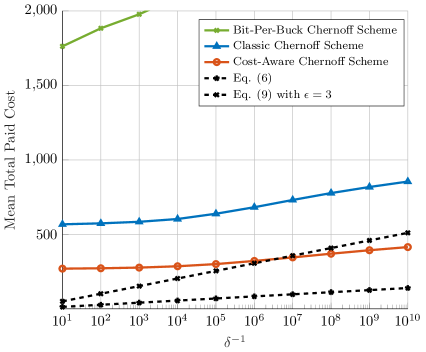
Figure 2: The expected total paid costs of the classic Chernoff and Cost-Aware Chernoff schemes. All samples are unit-variance, normally distributed with randomly drawn means.

V Conclusion

We introduced the NHSHT, a cost-aware variant of SHT in which actions carry non-homogeneous positive costs. We showed that minimizing expected total cost is followed by optimizing the ratio between the expected number of information bits gained per sample and the expected cost per sample (both conditioned on the action selection policy itself). Building on this principle, we adapted the Chernoff scheme to NHSHT while retaining its scaling laws. Empirically, the adapted policy outperforms both the classic Chernoff scheme and the “bit-per-buck” heuristic, reducing mean total paid cost by 50% and by an order of magnitude, respectively.

Appendix A Miscellaneous Proofs

A-A Bounding The Objective Function Using (5)

Here, we leverage the conditional expectation in (2) and combine it with (5). Specifically, each addend inside the sum in (5) bounds $\mathbb{E}_{N}\left[N|\theta=i\right]$, so

(2) $$\geq\frac{\mathbb{E}_{A}\left[c_{A}|\theta=i\right]\times\log\frac{1}{\delta}}{\max_{{\underline{\smash{\lambda}}}_{i}\in\operatorname{\mathcal{PS}}(|\mathcal{A}|)}{\min_{j\neq i}\mathbb{E}_{A\sim{\underline{\smash{\lambda}}}_{i}}\left[\mathcal{D}_{KL}(f_{i}^{A}\|f_{j}^{A})\right]}}$$

$$=\frac{\mathbb{E}_{A}\left[c_{A}|\theta=i\right]\times\log\frac{1}{\delta}}{\max_{{\underline{\smash{\lambda}}}_{i}\in\operatorname{\mathcal{PS}}(|\mathcal{A}|)}{I_{i}({\underline{\smash{\lambda}}}_{i})}}$$

$$=\frac{\log\frac{1}{\delta}}{\frac{\max_{{\underline{\smash{\lambda}}}_{i}\in\operatorname{\mathcal{PS}}(|\mathcal{A}|)}{I_{i}({\underline{\smash{\lambda}}}_{i})}}{\mathbb{E}_{A}\left[c_{A}|\theta=i\right]}}$$

$$=\frac{\log\frac{1}{\delta}}{\frac{\max_{{\underline{\smash{\lambda}}}_{i}\in\operatorname{\mathcal{PS}}(|\mathcal{A}|)}{I_{i}({\underline{\smash{\lambda}}}_{i})}}{\mathbb{E}_{A_{i}\sim{\underline{\smash{\lambda}}}_{i}}\left[c_{A_{i}}\right]}}$$

$$\geq\frac{\log\frac{1}{\delta}}{\max_{{\underline{\smash{\lambda}}}_{i}\in\operatorname{\mathcal{PS}}(|\mathcal{A}|)}\frac{I_{i}({\underline{\smash{\lambda}}}_{i})}{\mathbb{E}_{A_{i}\sim{\underline{\smash{\lambda}}}_{i}}\left[c_{A_{i}}\right]}}$$

A-B Proof of Lemma 1

With the new notation, (8) can be rewritten as

$$\begin{split}\max_{{\underline{\smash{\lambda}}}_{i}\in\mathbb{R}^{|\mathcal{A}|}}\quad&\frac{\min_{j\neq i}{\underline{\smash{d}}}_{ij}^{T}{\underline{\smash{\lambda}}}_{i}}{{\underline{\smash{c}}}^{T}{\underline{\smash{\lambda}}}_{i}}\\ \mathrm{s.t.}\quad&\begin{cases}{\underline{\smash{1}}}^{T}{\underline{\smash{\lambda}}}_{i}=1\\ {\underline{\smash{\lambda}}}_{i}\geq{\underline{\smash{0}}}\end{cases}\end{split}.$$ (11)

We now show equivalence. For any ${\underline{\smash{\nu}}}$ feasible in (11), the pair ${\underline{\smash{y}}}={\underline{\smash{\nu}}}/({\underline{\smash{c}}}^{T}{\underline{\smash{\nu}}})$ and $z=1/({\underline{\smash{c}}}^{T}{\underline{\smash{\nu}}})$ is feasible for the optimization problem in Lemma 1. The value of the objective function in the problem in Lemma 1 becomes $\min_{j\neq i}{\underline{\smash{d}}}_{ij}^{T}{\underline{\smash{\nu}}}/({\underline{\smash{c}}}^{T}{\underline{\smash{\nu}}})$ in this case, which is the same value the objective function in (11) obtains when setting ${\underline{\smash{\lambda}}}_{i}={\underline{\smash{\nu}}}$.

Assume ${\underline{\smash{y}}}$ and $z$ are feasible for the problem in Lemma 1. Note that $z={\underline{\smash{1}}}^{T}{\underline{\smash{y}}}\neq 0$ (otherwise, ${\underline{\smash{y}}}={\underline{\smash{0}}}$ and the constraint ${\underline{\smash{c}}}^{T}{\underline{\smash{y}}}=1$ does not hold). We observe that ${\underline{\smash{\nu}}}={\underline{\smash{y}}}/z\geq{\underline{\smash{0}}}$ is feasible for (11) as ${\underline{\smash{1}}}^{T}{\underline{\smash{\nu}}}={\underline{\smash{1}}}^{T}{\underline{\smash{y}}}\times\frac{1}{z}={\underline{\smash{1}}}^{T}{\underline{\smash{y}}}\times({\underline{\smash{1}}}^{T}{\underline{\smash{y}}})^{-1}=1$. Particularly, setting ${\underline{\smash{\lambda}}}_{i}={\underline{\smash{y}}}/z$ inside the objective function in (11) results in the value of $\min_{j\neq i}{\underline{\smash{d}}}_{ij}^{T}{\underline{\smash{y}}}$, which is the same value as of the objective function in Lemma 1.

References

- [1] T. M. Cover and J. A. Thomas, Elements of Information Theory (Wiley Series in Telecommunications and Signal Processing). USA: Wiley-Interscience, 2006.
- [2] A. Wald, “Sequential tests of statistical hypotheses,” The Annals of Mathematical Statistics, vol. 16, no. 2, pp. 117–186, 1945. [Online]. Available: http://www.jstor.org/stable/2235829
- [3] P. Armitage, “Sequential analysis with more than two alternative hypotheses, and its relation to discriminant function analysis,” Journal of the Royal Statistical Society. Series B (Methodological), vol. 12, no. 1, pp. 137–144, 1950. [Online]. Available: http://www.jstor.org/stable/2983839
- [4] H. Chernoff, “Sequential design of experiments,” The Annals of Mathematical Statistics, vol. 30, no. 3, pp. 755 – 770, 1959. [Online]. Available: https://doi.org/10.1214/aoms/1177706205
- [5] V. Dragalin, A. Tartakovsky, and V. Veeravalli, “Multihypothesis sequential probability ratio tests .I. asymptotic optimality,” IEEE Transactions on Information Theory, vol. 45, no. 7, pp. 2448–2461, 1999.
- [6] ——, “Multihypothesis sequential probability ratio tests. ii. accurate asymptotic expansions for the expected sample size,” IEEE Transactions on Information Theory, vol. 46, no. 4, pp. 1366–1383, 2000.
- [7] K. Cohen and Q. Zhao, “Active hypothesis testing for anomaly detection,” IEEE Transactions on Information Theory, vol. 61, no. 3, pp. 1432–1450, 2015.
- [8] L. Citron, K. Cohen, and Q. Zhao, “Anomaly search of a hidden markov model,” in IEEE International Symposium on Information Theory (ISIT), 2024, pp. 3684–3688.
- [9] M. Burnashev, “Data transmission over a discrete channel with feedback. random transmission time,” Problemy Peredachi Informatsii, vol. 12, 01 1976.
- [10] M. Naghshvar and T. Javidi, “Active sequential hypothesis testing,” The Annals of Statistics, vol. 41, no. 6, pp. 2703 – 2738, 2013. [Online]. Available: https://doi.org/10.1214/13-AOS1144
- [11] K. Gan, S. Jia, and A. Li, “Greedy approximation algorithms for active sequential hypothesis testing,” in Advances in Neural Information Processing Systems, M. Ranzato, A. Beygelzimer, Y. Dauphin, P. Liang, and J. W. Vaughan, Eds., vol. 34. Curran Associates, Inc., 2021, pp. 5012–5024. [Online]. Available: https://proceedings.neurips.cc/paper_files/paper/2021/file/27e9661e033a73a6ad8cefcde965c54d-Paper.pdf
- [12] G. Vershinin, A. Cohen, and O. Gurewitz, “Multi-stage active sequential hypothesis testing with clustered hypotheses,” 2025. [Online]. Available: https://arxiv.org/abs/2501.11459
- [13] E. C. Elumar, C. Tekin, and O. Yağan, “Multi-armed bandits with costly probes,” IEEE Trans. Inf. Theor., vol. 71, no. 1, p. 618–643, Jan. 2025. [Online]. Available: https://doi.org/10.1109/TIT.2024.3506866
- [14] Q. Xie, R. Astudillo, P. I. Frazier, Z. Scully, and A. Terenin, “Cost-aware bayesian optimization via the pandora’s box gittins index,” in Proceedings of the 38th International Conference on Neural Information Processing Systems, ser. NIPS ’24. Red Hook, NY, USA: Curran Associates Inc., 2025.
- [15] T. Banerjee and V. V. Veeravalli, “Data-efficient minimax quickest change detection,” in IEEE International Conference on Acoustics, Speech and Signal Processing (ICASSP), 2012, pp. 3937–3940.
- [16] Y. Hou, H. Bidkhori, and T. Banerjee, “Robust quickest change detection with sampling control,” 2024. [Online]. Available: https://arxiv.org/abs/2412.20207
- [17] N. K. Vaidhiyan and R. Sundaresan, “Active search with a cost for switching actions,” in Information Theory and Applications Workshop (ITA), 2015, pp. 17–24.
- [18] T. Lambez and K. Cohen, “Anomaly search with multiple plays under delay and switching costs,” IEEE Transactions on Signal Processing, vol. 70, pp. 174–189, 2022.
- [19] A. Caplin and M. Dean, “Revealed preference, rational inattention, and costly information acquisition,” American Economic Review, vol. 105, no. 7, p. 2183–2203, July 2015. [Online]. Available: https://www.aeaweb.org/articles?id=10.1257/aer.20140117
- [20] T. H. Cormen, C. E. Leiserson, R. L. Rivest, and C. Stein, Introduction to Algorithms, 3rd Edition. MIT Press, 2009. [Online]. Available: http://mitpress.mit.edu/books/introduction-algorithms
- [21] A. Leon-Garcia, Probability, Statistics, and Random Processes for Electrical Engineering, 3rd ed. Upper Saddle River, NJ: Pearson/Prentice Hall, 2008.
- [22] B. Nakiboğlu and R. G. Gallager, “Error exponents for variable-length block codes with feedback and cost constraints,” IEEE Transactions on Information Theory, vol. 54, no. 3, pp. 945–963, 2008.
- [23] M. Naghshvar and T. Javidi, “Supplement to “Active Sequential Hypothesis Testing”,” The Annals of Statistics, vol. 41, no. 6, pp. 2703 – 2738, 2013. [Online]. Available: https://doi.org/10.1214/13-AOS1144SUPP
- [24] S. Boyd and L. Vandenberghe, Convex Optimization. Cambridge University Press, 2004.