Resetting Induces Memory Loss in Non-Markovian Processes

Abstract

Stochastic resetting is a powerful strategy known to accelerate the first-passage time statistics of stochastic processes. While its effects on Markovian systems are well understood, a general framework for non-Markovian dynamics is still lacking, mostly due to its mathematical complexity. Here, we present an analytical and numerical framework to study non-Markovian processes under resetting, focusing on the first-passage properties of escape kinetics from metastable states. We show that resetting disrupts the inherent time correlation, inducing Markovianity, thereby leading to an efficient escape mechanism. This work, therefore, provides a much needed theoretical approach for incorporating resetting into complex chemical and biological processes, which follow non-Markovian dynamics.

I Introduction

Escape from a metastable state is a profoundly interesting and important topic in physics, chemistry, and biology hanggi1986 ; hanggi1990 ; atkins2023 , typically associated with phenomena like rapid bond breaking, anomalous diffusion, dynamics of protein conformation, polymer translocation, transportation through crowded environments and complex chemical reactions sung1996 ; lu1998 ; edman1999 ; flomenbom2005 ; min2005 ; min2006 ; english2006 ; chaudhury2006 ; chaudhury2007 ; goychuk2007 ; dubbeldam2007 ; wiggin2008 ; panja2010 ; chatterjee2010 ; sharma2010 ; sharma2012subdiffusion ; batra2021 ; batra2022 . The underlying dynamics are often non-Markovian, induced by temporally correlated fluctuations that give rise to a memory kernel of collision history, in turn slowing down the process sung1996 ; min2006 ; chaudhury2006 ; chaudhury2006 ; goychuk2007 ; dubbeldam2007 ; chaudhury2007 ; balakrishnan2008 ; chatterjee2010 ; panja2010 ; sharma2010 ; saha2024 . This results in a broad first-passage time (FPT) distribution with heavy tails, representing non-exponential decay, characteristic of rare events hanggi1990 ; chaudhury2006 ; batra2022 ; barbier2024 .

Since these rare events are few and far between with long wait times, alternative approaches focus on re-designing the system such that transitions away from the target are halted and then resumed from a more favourable state. This strategy, called stochastic resetting, has been proven to lead to efficient transport and target search in a variety of disciplines evans2011 ; evans2011diffusion-optimal ; pal2015 ; roldan2016 ; pal2017 ; tal2020 ; ray2020 ; ray2020space-dependent ; evans2020 ; ramoso2020 ; gupta2022 ; santra2022 ; blumer2022 . Specifically, it has been shown to accelerate first-passage time, as trajectories that drift too far from the target are also reset. The usefulness of resetting in Markovian systems has, therefore, been well established evans2011 ; evans2011diffusion-optimal ; pal2015 ; roldan2016 ; pal2017 ; tal2020 ; gupta2022 ; ray2020 ; ray2020space-dependent ; evans2020 ; ramoso2020 ; cantisan2021 ; santra2022 ; blumer2022 ; singh2025 ; evans2025stochastic . However, its application in non-Markovian systems remains a challenge due to its inherent complexity and lack of proper analytical framework.

Motivated by this, in this letter, we present a detailed analytical and numerical approach to implement stochastic resetting in a non-Markovian system set up to study escape kinetics. This system, as such, can be described by the generalized Langevin equation (GLE) as it inherently incorporates temporal correlations in fluctuations, resulting in the trajectory history affecting the future state of the system balakrishnan2008 . Apart from providing a framework for studying temporally correlated dynamics under stochastic resetting, our study also reveals that repeated resetting leads to a transition from the non-Markovian to the Markovian regime. This transition is characterised by a marked change in the FPT distribution, from heavy-tail to near-exponential, essentially showing a breaking of long-term correlation. Additionally, we also provide an optimal reset protocol that enhances the escape process. This work, therefore, lays a general foundation for studying efficient transport mechanisms in various chemical and biological processes, whose dynamics are inherently non-Markovian.

II Analytical framework for resetting in non-Markovian systems

Let us now define the mathematical framework. Consider a particle of mass $m$ performing anomalous diffusion in a one-dimensional potential well under thermal fluctuations in a bath of temperature $T$. The dynamics of such a particle in the presence of temporally correlated noise are governed by the following GLE,

$$m\ddot{x}(t)=-\zeta\int_{0}^{t}dt^{\prime}K(t-t^{\prime})\dot{x}(t^{\prime})-\frac{dU(x)}{dx}+\theta(t)$$ (1)

where, $\zeta$ is the friction coefficient and $U(x)$ represents the potential well in which the particle is diffusing. $\theta(t)$ is the temporally correlated fractional Gaussian noise (fGn), with $\langle\theta(t)\rangle=0$ mandelbrot1968 . This fGn is related to the memory kernel $K(t-t^{\prime})$ through the fluctuation-dissipation relation $\langle\theta(t)\theta(t^{\prime})\rangle=\zeta k_{\text{B}}TK(t-t^{\prime})$, where, $K(t-t^{\prime})=2H(2H-1)|t-t^{\prime}|^{2H-2}$, $k_{\text{B}}$ is the Boltzmann constant and $H$ is the Hurst index parameter ($\frac{1}{2}\leq H<1$) that determines the strength of the correlation. $H=1/2$ corresponds to white noise, representing the Markovian limit where the fluctuations are uncorrelated. Here, we consider a power-law memory kernel as earlier studies have shown that it gives good agreement with experimental results, particularly for chemical and biological systems min2005 ; chaudhury2006 ; min2006 ; chaudhury2007 ; chaudhury2007modulation ; chaudhury2008 ; chatterjee2010 ; sharma2010 ; bhattacharyya2012 .

For simplicity, the potential energy is taken to be $U(x)=\frac{1}{2}m\omega^{2}x^{2}$, i.e., harmonic in nature, where $\omega$ is the barrier frequency. In the overdamped limit, Eq. (29) can be written as

$$m\omega^{2}x(t)=-\zeta\int_{0}^{t}dt^{\prime}K(t-t^{\prime})\dot{x}(t^{\prime})+\theta(t)$$ (2)

The corresponding Fokker-Planck equation (FPE) in terms of the probability of the particle to be at $x$ at time $t$, starting from $x_{0}$ can be derived from Eq. (2) (see Appendix D) and is given by

$$\frac{\partial P(x,t|x_{0})}{\partial t}=\eta(t)\bigg[\frac{\partial}{\partial x}x+\frac{k_{\text{B}}T}{m\omega^{2}}\frac{\partial^{2}}{\partial x^{2}}\bigg]P(x,t|x_{0})$$ (3)

with $P(x,0|x_{0})=\delta(x-x_{0})$ as the initial condition. Here, $\eta(t)=-\frac{\dot{\chi}(t)}{\chi(t)}$ is the time-dependent diffusion coefficient, where $\chi(t)=E_{b}\big[-\big(\frac{t}{\tau_{0}}\big)^{b}\big]$, $\tau_{0}=\Big[\frac{\zeta\Gamma(2H+1)}{m\omega^{2}}\Big]^{1/b}$, $b=2-2H$. $E_{\alpha}(-z)=\sum_{k=0}^{\infty}(-1)^{k}\frac{z^{k}}{\Gamma(\alpha k+1)}$ is known as the Mittag-Leffler function haubold2011 .

The particle diffuses in the well and tends to escape from it by the influence of thermal fluctuations. We set an absorbing boundary at $x=x_{a}$, and as the particle hits this boundary, it is assumed to escape the well. Here, in this work, we are primarily interested in finding the mean first-passage time (MFPT), which is the average time it takes to escape the well. We show that the MFPT can be influenced by restarting the dynamics from $x=x_{r}$ with a constant rate $r$ at random instants of time $t$, drawn from a Poissonian distribution $re^{-rt}$ evans2011 ; evans2011diffusion-optimal . In such a scenario, the FPE can be rewritten as

$$\frac{\partial P(x,t|x_{0})}{\partial t}=\eta(t)\bigg[\frac{\partial}{\partial x}x+\frac{k_{\text{B}}T}{m\omega^{2}}\frac{\partial^{2}}{\partial x^{2}}\bigg]P(x,t|x_{0})-rP(x,t|x_{0})+r\delta(x-x_{r})$$ (4)

The second and third terms on the right-hand side correspond to the loss and gain of probability due to the reset. A probability current is generated from the reset position, giving rise to a non-equilibrium stationary state (NESS) at long times.

The next step is to solve Eq. (4) to find $P(x,t|x_{0})$ for $x\in(-\infty,\infty)$. Once we solve this, we can calculate the survival probability, given by

$$S(t|x_{0})=\int_{-\infty}^{x_{a}}P(x,t|x_{0})dx.$$ (5)

It represents the probability that the particle has survived until time $t$ before getting absorbed by the boundary at $x_{a}$. The idea of survival probability is well-known in chemical kinetics, and we are interested in knowing how it differs when stochastic resetting is considered. After obtaining $S(t|x_{0})$, we evaluate the FPT distribution, corresponding to the times required by the particles to hit the boundary. This can be calculated as

$$f(t|x_{0})=-\frac{d}{dt}S(t|x_{0}).$$ (6)

Finally, we calculate mean escape time, or the MFPT, which is the first moment of $f(t|x_{0})$, given by,

$$\big\langle T\big\rangle=\int_{0}^{\infty}t\penalty 10000\ f(t|x_{0})dt=\int_{0}^{\infty}S(t|x_{0})dt$$ (7)

using the conditions $S(0|x_{0})=1$ and $S(\infty|x_{0})=0$.

We begin by solving Eq. (4) to get the expression for $P(x,t|x_{0})$ in the presence of resetting. The solution can be obtained from the last renewal equation evans2011diffusion-optimal ; evans2020 ,

$$P(x,t|x_{0})=e^{-rt}G(x,t|x_{0},0)+r\int_{0}^{t}d\tau e^{-r\tau}G(x,\tau|x_{r})$$ (8)

The first term on the right-hand side corresponds to the case when no resetting event happens during the entire motion. The second term suggests that the last resetting has occurred at time $\tau$ to the position $x_{r}$, followed by diffusion for the rest of the interval $t-\tau$, starting from $x_{r}$. Here $G(x,t|x_{0},0)$ is the Green’s propagator that defines the probability of transition from $x_{0}$ at $t=0$ to $x$ at time $t$. It should be noted that, although the dynamics are non-Markovian, the renewal equation still holds because the reset time follows a Poissonian distribution, which is independent of the system’s dynamics. The propagator, $G(x,t|x_{0},0)$, then satisfies the equation:

$$\bigg(\frac{\partial}{\partial t}-\mathcal{L}\bigg)G(x,t-t^{\prime}|x^{\prime})=\delta(x-x^{\prime})\delta(t-t^{\prime})$$ (9)

where the operator $\mathcal{L}\equiv\eta(t)\Big[\frac{\partial}{\partial x}x+\frac{k_{\text{B}}T}{m\omega^{2}}\frac{\partial^{2}}{\partial x^{2}}\Big]$. The solution of this equation is (see Appendix E) chatterjee2010

$$G(x,t|x_{0},0)=\sqrt{\frac{m\omega^{2}}{2\pi k_{\text{B}}T\big(1-\chi^{2}(t)\big)}}\exp{\bigg[-\frac{m\omega^{2}\big(x-x_{0}\chi(t)\big)^{2}}{2k_{\text{B}}T\big(1-\chi^{2}(t)\big)}\bigg]}.$$ (10)

Next, we solve Eq. (8) to understand how the dynamics evolve with time. However, the task is not easy due to the complexity of the Green’s function. We solved it numerically in Mathematica Mathematica and showed the results for $P(x,t|x_{0})$ in FIG. 1 for different values of the Hurst index ($H$) and the reset rate ($r$). $P(x,t|x_{0})$ is plotted at different times to show the temporal evolution of the distribution and the emergence of the NESS. In the Markovian case ($H=0.5$), as shown in FIG. 1 A, the system reaches steady state (SS) even when no resetting is considered. This SS is due to the nature of the potential well, which suggests that the particle is confined in a stable equilibrium. When resetting is considered, the system again shows an SS, but now the distribution has shifted towards the reset position, with a sharp peak at $x=x_{r}$, as shown in FIG. 1 B. This SS is a well-known property of systems under stochastic resetting evans2011 ; evans2011diffusion-optimal ; pal2015 ; roldan2017 ; tal2020 ; evans2020 ; gupta2022 , which can be evaluated by taking the $t\to\infty$ limit in Eq. (4). The reason behind the SS is that, as we repeatedly restart the dynamics, the particles cannot move away from $x_{r}$ and instead keep diffusing around the neighbourhood of $x_{r}$, resulting in a stationary distribution in the long term.

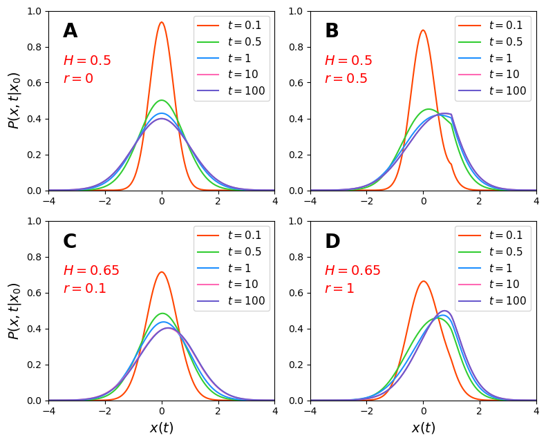
Figure 1: Probability density $P(x,t|x_{0})$ corresponding to the escape dynamics governed by GLE, subjected to stochastic resetting. Distributions at different noise strengths and reset rates are shown. (A) and (B) shows the most probable positions for $H=0.5$ in the absence and presence of resetting. (C) and (D) shows the same for $H=0.65$ and with low and high reset rates.

In FIG. 1 C and 1 D, we have shown $P(x,t|x_{0})$ for the non-Markovian case ($H=0.65$) with resetting. Here again, the system shows an SS, but the process is relatively slower compared to Markovian dynamics. This is because, particles undergoing a non-Markovian process diffuse at a slower rate saha2024 depending on the correlation strength defined by $H$. In the figure, we compare the dynamical effects of resetting for different values of $r$. For low $r$, the SS is formed at a position that is away from the resetting point, as the particle tries to drift towards the bottom of the well. However, when the particle is being reset with a higher $r$, the SS is formed very close to the reset position, $x_{r}$. Interestingly, there are no sharp peaks in the distribution of the non-Markovian case (see FIGs. 1 C and 1 D), likely because the dynamics are summed over the relaxation time scale, and the sharp characteristics that are supposed to appear near $x_{r}$ due to reset, is smoothened out.

Figure 2: Simulated trajectories and corresponding distributions with and without resetting. (A) Sample trajectories following the dynamics governed by Eq. (2) for $H=0.65$ and $r=0$. (B) Comparison between analytical (solid lines) and simulated (histograms) distributions $P(x,t|x_{0})$. Histograms are obtained from $10^{4}$ simulated trajectories with $0.002$ time steps. (C) Sample trajectories illustrating diffusion with stochastic resetting, where $r=1$, $x_{r}=1$ and $H=0.65$. (D) Comparison between the analytical and numerical results of $P(x,t|x_{0})$ in the presence of resetting.

The dynamics are validated by numerical simulation of Eq. (2) in the presence of resetting. The discretization of GLE using the fractional Caputo derivative gorenflo1997 ; mainardi2007 ; luchko2020 , and the simulation techniques are described in the Appendix (B and C). A total of $10^{4}$ trajectories are simulated with a time step of 0.002 for both resetting and non-resetting cases. The resulting output trajectories and the corresponding histograms are shown in FIG. 2. In FIG. 2 A, three sample trajectories without any resetting are shown. The corresponding distributions are shown in FIG. 2 B at different time instants. The effects of stochastic resetting on the trajectories are shown in FIG. 2 C. Positions of the particles are reset to $x_{r}$ at random times from where a new diffusion starts and the corresponding distributions are shown in FIG. 2 D. The simulated histograms show good agreement with analytical results, obtained by solving Eq. (8), both in the Markovian and non-Markovian regimes. Simulation codes are available at https://github.com/saha-debasish/escape-kinetics-with-resetting.git on Github.

Having obtained the position probability distribution, $P(x,t|x_{0})$, we now focus on evaluating the survival probability, $S(t|x_{0})$, as defined in Eq. (5). By using this definition in Eq. (8), we get

$$S(t|x_{0})=e^{-rt}\penalty 10000\ I(t|x_{0})+r\int_{0}^{t}d\tau\penalty 10000\ e^{-r\tau}\penalty 10000\ I(\tau|x_{r})$$ (11a)

where

$$\begin{split}I(t|x_{0})&=\int_{-\infty}^{x_{a}}dx\penalty 10000\ G(x,t|x_{0})=\frac{1}{2}\Bigg[1+\text{erf}\bigg(\sqrt{\frac{m\omega^{2}}{2k_{\text{B}}T}}\penalty 10000\ \frac{x_{a}-x_{0}\chi(t)}{\sqrt{1-\chi^{2}(t)}}\bigg)\Bigg]\end{split}$$ (11b)

Analytical forms for the survival probability can be obtained in the short and long time limits (See Appendix A for details). The effects of resetting on $S(t|x_{0})$ are shown in FIG. 3 A for different reset rates ($r$) at $H=0.65$, keeping the absorbing boundary at $x_{a}=3$, and the reset position $x_{r}=1$. At early times, $S(t|x_{0})$ is unity, indicating that the particle is entirely inside the well. This probability gradually decreases over time, showing the escape of particles from the well. FIG. 3 A shows that at any time instant, $S(t|x_{0})$ in the presence of resetting has relatively lower magnitude in comparison to the non-resetting case. It also shows that the $S(t|x_{0})$ decreases with increasing reset rates. This implies that particles escape the well faster upon resetting. However, there exists an optimal reset condition for efficient escape, beyond which resetting can in fact lead to longer escape times compared to the non-resetting case. In FIG. 3 B, we have shown the change in survival probability with time at different values of the correlation strength (via parameter $H$), keeping $r$ fixed at 0.2. $S(t|x_{0})$ shows rapid decrease for the white noise limit, i.e., $H=0.5$. But, as $H$ increases, the decay becomes relatively slower. This is typical for non-Markovian processes, as higher $H$ implies more strongly correlated dynamics leading to slower diffusion and, as a result, a higher chance of survival within the well. In such highly correlated systems, particles take longer to escape the well, resulting in longer reaction times.

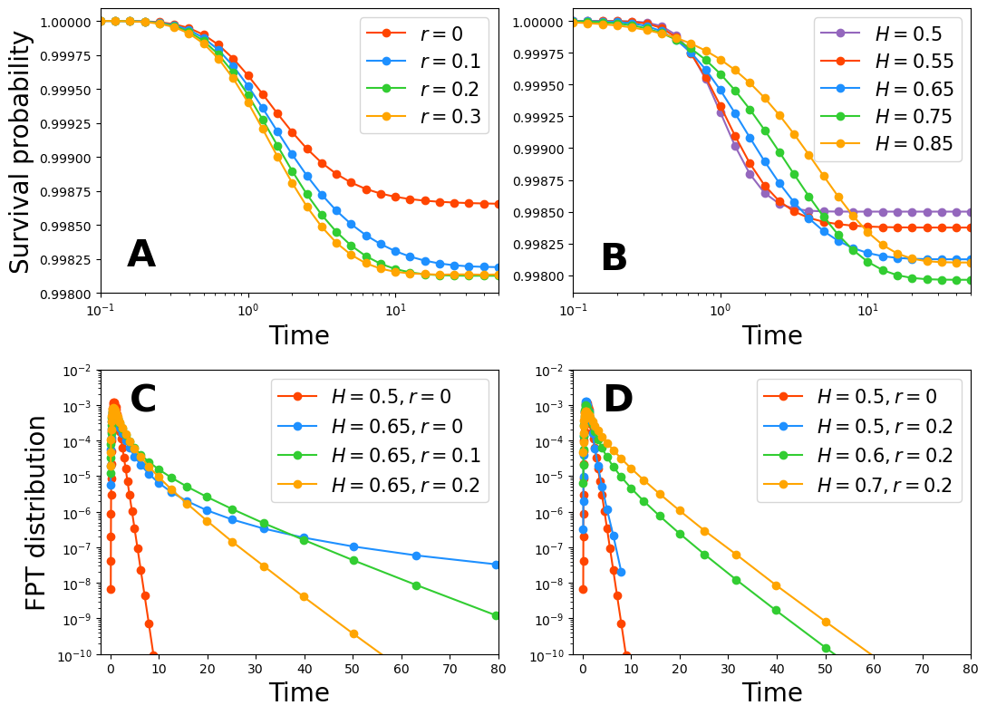
Figure 3: Survival probabilities as a function of time at (A) different values of $r$ keeping $H=0.65$, (B) different values of $H$ keeping $r=0.2$. (C) FPT distributions at different reset rates ($r$), keeping $H=0.65$. (D) FPT distributions at different $H$, keeping $r=0.2$. Orange curves in (C) and (D) correspond to the FPT distribution in the Markovian limit, and no reset condition. The reset position is $x_{r}=1$, and the absorbing boundary $x_{a}=3$ for the cases.

Next, we focus on the FPT distribution and MFPT of the escape process to not only understand how resetting facilitates faster escape in a non-Markovian system, but also how it affects memory. It is well-known that the FPT distribution, $f(t|x_{0})$, for non-Markovian dynamics displays non-exponential decay, particularly when dealing with complex chemical and biological processes chaudhury2006 ; chaudhury2007 ; chaudhury2008 ; min2008 ; hu2010 ; nyberg2016 . This non-exponential and slow long tailed decay in $f(t|x_{0})$ implies delayed escape from the well, a typical characteristic of rare events hanggi1990 ; chaudhury2006 ; barbier2024 , as is also the case with escape kinetics of a non-Markovian systems in the absence of resetting (see the plot for $H=0.5$ and $r=0$ in FIG. 3 C). In the presence of resetting, however, the FPT distribution becomes narrower with increasing reset rate, as seen in FIG. 3 C, showing a faster elimination of particles from the well. A similar effect of resetting on survival probability and FPT distribution was observed for non-linear diffusion in porous media lenzi2023 .

Further, in addition to the FPT distribution becoming narrower with resetting introduced in non-Markovian systems, it interestingly also shows a transition from non-exponential decay to near-exponential decay (see the plots for $H>0.5$ and $r>0$ in FIG. 3 C and FIG. 3 D). This transition to near-exponential decay implies a loss of memory, similar to the uncorrelated dynamics of Markovian systems. This happens because as we reset the dynamics, the temporal correlation breaks, and the memory of past events vanishes. In such a scenario, reset dominates over memory, and the particles start escaping the well at random times coming from a Poissonian distribution, giving rise to an exponential decay. However, at short times, the distributions continue to be non-exponential as particles can still diffuse in these timescales and resetting is less probable. This transition has real significance in understanding the dynamics of escape processes in such complex environments. Memory tends to slow down the process; the stronger the memory, the slower the dynamics. Stochastic resetting, however, erases memory by breaking the temporal correlation, leading to efficient escape from the well, which is reflected in the survival probabilities and the FPT distributions. Further, although frequent resetting leads to erasure of memory to some extent, the effect of correlation is still felt on the escape kinetics. This can be seen in FIG. 3 D, where increasing the Hurst parameter while keeping $r$ fixed at 0.2 still leads to a broadening of the FPT distribution.

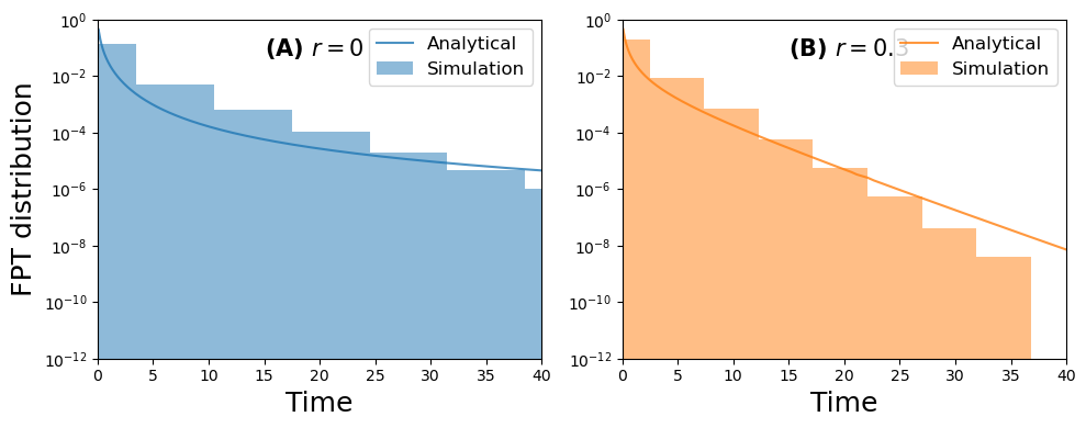
Figure 4: Numerically calculated FPT distribution and its comparison with analytical results. Histograms were evaluated from $10^{8}$ trajectories, with $0.002$ time interval. Simulations were performed at different values of $r$, keeping $H=0.65$, $x_{a}=1$ and $x_{r}=0.5$.

The FPT distributions are validated by performing numerical simulations following the same method as discussed earlier, but with an additional absorbing boundary at $x=x_{a}$ (see Sections II and III in SI). We simulated $10^{8}$ trajectories to capture the rare events and the effects of resetting on the FPT distributions. As seen in FIG. 4, simulations show very good agreement with analytical results. They capture the long tailed or near-exponential decay in the FPT distribution of non-Markovian dynamics in the absence and presence of resetting, respectively. Interestingly, the computation time also significantly reduced to 6 hours with resetting ($r=0.3$), compared to over 14 hours when no resetting was considered. Simulation codes are available at https://github.com/saha-debasish/escape-kinetics-with-resetting.git on Github.

So far, we have studied the effect of resetting on the first-passage properties of non-Markovian dynamics. Now, we focus on understanding the dependence of MFPT on the reset parameters and finding an optimal reset protocol. MFPT, as given by Eq. (7), is defined as the first-moment of the FPT distribution, which can also be calculated by integrating $S(t|x_{0})$ over $t\in[0,\infty)$. Since, we have evaluated $S(t|x_{0})$ in a finite range of time, we cannot integrate over the entire time range. Instead, we integrate $S(t|x_{0})$ in the same range as shown in FIG. 5. This sum of $S(t|x_{0})$ is then analogous to the MFPT (not the exact MFPT). It should, however, be noted that $S(t|x_{0})$ beyond this range is constant, and the only change occurring is within this limit. Therefore, considering the changes in this particular range is sufficient to describe the effects of reset on MFPT. Fig. 5 A shows that the survival probability decreases with $r$ up to an optimal value, beyond which it starts increasing monotonically. Similar non-monotonous behaviour is reflected in the MFPT plot, shown in Fig. 5 B. This phenomenon of reducing MFPT by resetting the dynamics is well known and has been observed in many other physical and biological systems evans2011 ; evans2011diffusion-optimal ; pal2015 ; pal2017 ; tal2020 ; ray2020 ; ray2020space-dependent ; evans2020 ; gupta2022 ; blumer2022 . The dotted horizontal line represents MFPT in the absence of resetting. Therefore, resetting the particle with a suitable reset rate can reduce the escape time, leading to faster escape from the well. However, resetting the particle more frequently (higher $r$) can delay the process as it does not get sufficient time to diffuse away from the reset position, hindering it from reaching the absorbing boundary. In this analysis, we set $\zeta=1$, $\omega=1$, and $m=1$, which are arbitrary but can capture the effect of resetting in such a system.

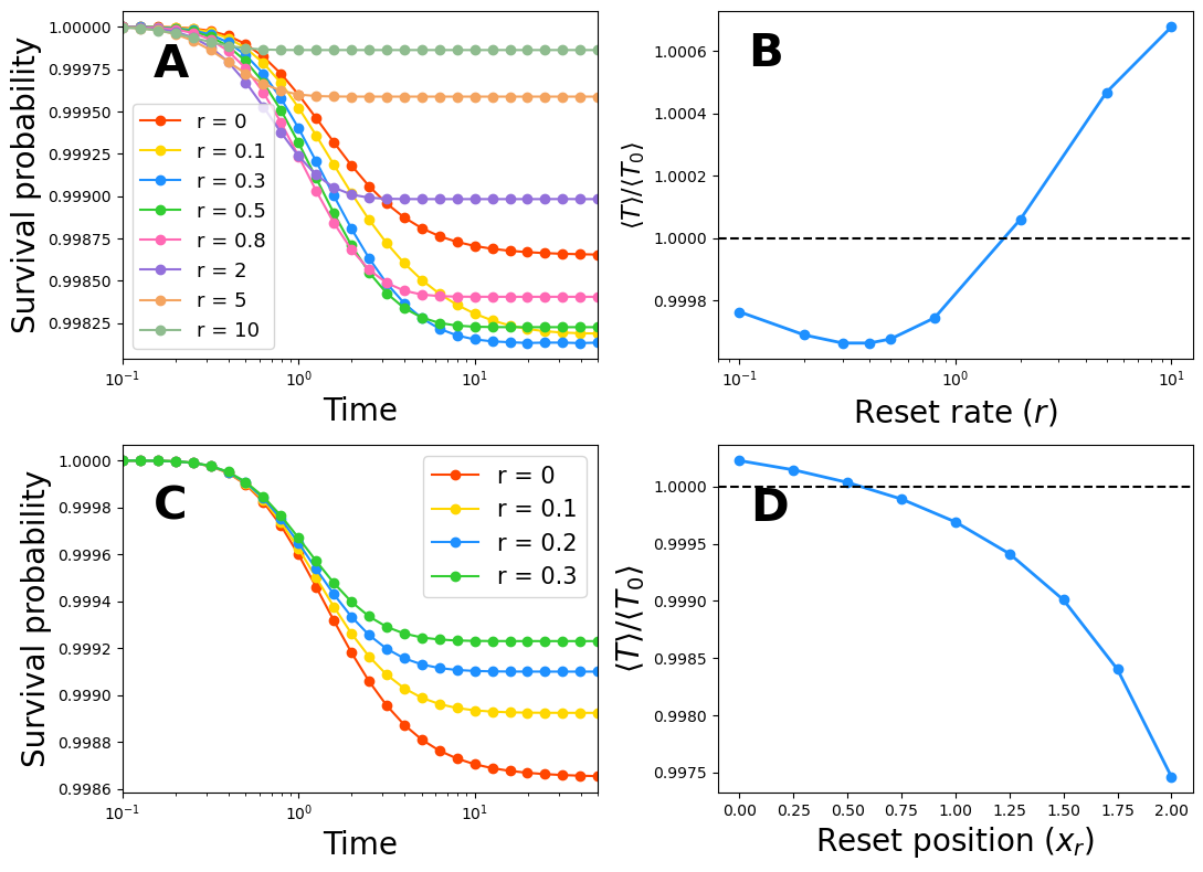
Figure 5: (A) $S(t|x_{0})$ at different values of $r$ with $x_{r}=1$. (B) MFPT as a function of $r$ with $x_{r}=1$. (C) $S(t|x_{0})$ at different $r$ with $x_{r}=0$. (D) MFPT as a function of $x_{r}$ keeping $r=0.2$. In all the figures, we fixed $H=0.65$ and $x_{a}=3$. The horizontal dashed lines show the MFPT without resetting.

It is also to be noted that resetting the particle at the bottom of the well has higher survival compared to the non-resetting case. The survival probability, in fact, continues to increase as we increase the reset rate, as shown in FIG. 5 C. Therefore, the escape process in the presence of resetting has a strict dependence on the reset position as well singh2025 . To explore this, we also studied MFPT as a function of $x_{r}$ at a fixed $r=0.2$, as shown in FIG. 5 D, to find a preferable reset position to get an efficient escape from the well. Particles that are at the stable equilibrium position (potential minimum) take time to gain kinetic energy from the surroundings to escape from the well. During the diffusion process, the majority of its lifetime is spent near the bottom. As we reset the dynamics from the minimum, the particle loses all the kinetic energy gained during its diffusive phase and repeats the same process from where it was started, effectively delaying the escape. Therefore, to achieve an efficient escape mechanism, the dynamics should restart with an initial kinetic energy by resetting the particle away from the minimum.

III Conclusions

We formulate an analytical and numerical approach to incorporate stochastic resetting in non-Markovian systems, which are known to carry memory of past events, characterized by delayed escape from metastable states. The presence of heavy tails in the FPT distribution, representative of delayed escape, is replaced by faster escape spurred by stochastic resetting. Most importantly, we uncover a crossover between non-Markovian and Markovian characteristics, symbolising a memory break when the dynamics are restarted. Our study also provides an optimal reset condition for the most efficient escape from the well. This work, therefore, not only fills a crucial gap in the literature by incorporating stochastic resetting in memory-driven dynamics, but is also highly relevant in real systems like rapid bond-breaking, polymer translocation, anomalous diffusion and transportation in crowded environments, among others.

Appendix A Approximations in short and long time limits

The survival probability is calculated as

$$S(t|x_{0})=e^{-rt}\penalty 10000\ I(t|x_{0})+r\int_{0}^{t}d\tau\penalty 10000\ e^{-r\tau}\penalty 10000\ I(\tau|x_{r})$$ (12)

where

$$I(t|x_{0})=\int_{-\infty}^{x_{a}}dx\penalty 10000\ G(x,t|x_{0})=\frac{1}{2}\Bigg[1+\text{erf}\bigg(\sqrt{\frac{m\omega^{2}}{2k_{\text{B}}T}}\penalty 10000\ \frac{x_{a}-x_{0}\chi(t)}{\sqrt{1-\chi^{2}(t)}}\bigg)\Bigg]$$ (13)

We can now approximate $I(t|x_{r})$ inside the integral of Eq. (12) to obtain its expression in the short and long time limits.

A.1 Short-time limit

In the small time limit, $\chi(t)$ can be approximated as $\chi(t)\approx 1-a_{1}t^{b}$ where $a_{1}=\frac{\tau_{0}^{b}}{\Gamma(3-2H)}$. We used this expression in $I(t|x_{r})$ which results in

$$I(t|x_{r})\approx\frac{1}{2}\Bigg[1+\text{erf}\bigg(\sqrt{\frac{m\omega^{2}}{2k_{\text{B}}T}}\penalty 10000\ \frac{x_{a}-x_{r}+a_{1}x_{r}t^{b}}{\sqrt{2a_{1}t^{b}-a_{1}^{2}t^{2b}}}\bigg)\Bigg]=I_{1}(t|x_{r})$$ (14)

This simplifies the expression of the survival probability in the short time limit and is then given by

$$S(t|x_{0})\approx e^{-rt}\penalty 10000\ I(t|x_{0})+r\int_{0}^{t}d\tau\penalty 10000\ e^{-r\tau}\penalty 10000\ I_{1}(\tau|x_{r})$$ (15)

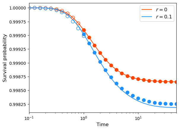
Figure 6: Comparison of survival probabilities calculated from the renewal equation (solid lines) and its approximations for the short (empty circles) and long (filled circles) time limits that are shown in Eq. (14) and (16), respectively.

A.2 Long-time limit

In the long time limit, $\chi(t)$ can be approximated as $\chi(t)\approx a_{2}t^{b}$, where $a_{2}=\frac{\tau_{0}^{b}}{\Gamma(2H-1)}$ chatterjee2010 . Incorporating this function in $I(t|x_{r})$ leads to

$$I(t|x_{r})\approx\frac{1}{2}\Bigg[1+\text{erf}\bigg(\sqrt{\frac{m\omega^{2}}{2k_{\text{B}}T}}\penalty 10000\ \Big[x_{a}-x_{r}a_{2}t^{-b}+\frac{1}{2}x_{a}a_{2}^{2}t^{-2b}\Big]\bigg)\Bigg]=I_{2}(t|x_{r})$$ (16)

Therefore, the survival probability in the long-time limit changes to

$$S(t|x_{0})\approx e^{-rt}\penalty 10000\ I(t|x_{0})+r\int_{0}^{t}d\tau\penalty 10000\ e^{-r\tau}\penalty 10000\ I_{2}(\tau|x_{r})$$ (17)

We show survival probability calculated following the renewal equation and its approximations in the short and long time regimes (Eqs. (15) and (17), respectively) in Fig. 6.

Appendix B Numerical solution

In this section, we formulate a numerical method to solve the generalized Langevin equation (Eq. ( 2) in the main text) and validate the effect of stochastic resetting over diffusion in a potential well in the non-Markovian limit.

The GLE describing the equation of motion of the particle is

$$m\omega^{2}x(t)=-\zeta\int_{0}^{t}dt^{\prime}K(t-t^{\prime})\dot{x}(t^{\prime})+\xi(t)$$ (18)

where $K(t-t^{\prime})$ is the power-law memory kernel defined as

$$K(t-t^{\prime})=2H(2H-1)|t-t^{\prime}|^{2H-2}$$ (19)

Using Eq. (19) in Eq. (18), we get

$$m\omega^{2}x(t)=-\frac{A}{\Gamma(1-\alpha)}\int_{0}^{t}dt^{\prime}\frac{\dot{x}(t^{\prime})}{(t-t^{\prime})^{\alpha}}+\xi(t)$$ (20)

Now we use the Caputo derivative gorenflo1997 , which is defined for order $\alpha$ as

$$^{C}\mathcal{D}^{\alpha}_{0}\big(x(t)\big)=\frac{1}{\Gamma(1-\alpha)}\int_{0}^{t}dt^{\prime}\frac{\dot{x}(t^{\prime})}{(t-t^{\prime})^{\alpha}}$$ (21)

Using this definition of Caputo derivative defined in Eq. (21) in Eq. (20), we get

$$^{C}\mathcal{D}^{\alpha}_{0}\big(x(t)\big)=\frac{1}{A}\Big(-m\omega^{2}x(t)+\sigma\dot{B}_{H}\Big)$$ (22)

Now, the fractional integral of order $\alpha$ is defined by gorenflo1997

$$^{C}\mathcal{J}^{\alpha}_{0}\big(x(t)\big)=\frac{1}{\Gamma(\alpha)}\int_{0}^{t}dt^{\prime}(t-t^{\prime})^{\alpha-1}x(t^{\prime})$$ (23)

Integrating Eq. (22) with the Caputo integral defined in Eq. (23) and making use of the fundamental theorems of fractional calculus luchko2020 ; mainardi2007

$${}^{C}\mathcal{D}^{\alpha}_{0}\big(x(t)\big)=\penalty 10000\ ^{C}\mathcal{J}^{1-\alpha}_{0}\frac{dx}{dt}$$ (24a)

$${}^{C}\mathcal{J}^{\alpha}_{0}\penalty 10000\ {}^{C}\mathcal{D}^{\alpha}_{0}\penalty 10000\ x(t)=x(t)-x(0)$$ (24b)

we get,

$$x(t)=x(0)-\frac{1}{A}\Bigg[\frac{m\omega^{2}}{\Gamma(\alpha)}\int_{0}^{t}dt^{\prime}(t-t^{\prime})^{\alpha-1}x(t^{\prime})+\frac{\sigma}{\Gamma(\alpha)}\int_{0}^{t}(t-t^{\prime})^{\alpha-1}dB_{H}\Bigg]$$ (25)

We consider

$$G(t)=\frac{\sigma}{\Gamma(\alpha)}\int_{0}^{t}(t-t^{\prime})^{\alpha-1}dB_{H}$$ (26)

where $G(t)$ is a Gaussian process of zero mean, as described in li2017 ; fang2020 ; batra2022 . As shown in li2017 , for $\alpha=2-2H$ and $\sigma=\frac{\sqrt{2}}{\sqrt{\Gamma(2H+1)}}$, the process $G(t)\overset{d}{=}\beta_{H}B_{1-H}$, where $\beta=\frac{\sqrt{2}}{\sqrt{\Gamma(3-2H)}}$ and $\overset{d}{=}$ defines that both the processes have same distribution. Hence, $G(t)$ is a fractional Brownian motion process with Hurst index $1-H$.

Now, we discretize Eq. (25) by splitting the total time $t$ into $n$ equal segments with segment width of $\Delta t=\frac{t}{n}$. Approximating the integral in Eq. (25) in the range between $(j-1)\Delta t$ and $j\Delta t$, and considering the function $x(t)$ as $x_{j-1}$, we get

$$x_{n}=x(0)+\frac{1}{A}\Bigg[-\frac{m\omega^{2}}{\Gamma(\alpha)}\sum_{j=1}^{n}x_{j-1}\int_{(j-1)\Delta t}^{j\Delta t}\big(n\Delta t-t^{\prime}\big)dt^{\prime}+G(n\Delta t)\Bigg]$$ (27)

Solving the integration, finally, we get,

$$x_{n}=x(0)+\frac{1}{A}\Bigg[-\frac{m\omega^{2}(\Delta t)^{2}}{\Gamma(\alpha+1)}\sum_{j=1}^{n}x_{j-1}\Big\{\big(n-j+1\big)^{\alpha}-\big(n-j\big)^{\alpha}\Big\}+G(n\Delta t)\Bigg]$$ (28)

This is the final equation to simulate the trajectories and verify their dynamics.

Appendix C Simulation steps

In section B, we discussed the method that we used to discretize the generalized Langevin equation (Eq. (18)) using Caputo derivative, which reduced to a discretized form mentioned in Eq. (28). This equation is used to simulate trajectories of particles influenced by correlated fluctuations and the potential well. The simulation techniques are described as follows:

1. We created a two-dimensional numpy array of dimension $(ntrajs\times N)$, where $ntrajs$ is the number of trajectories, and $N$ is the total number of time steps for each trajectory. All the trajectories were started from the origin at $t=0$.

2. Trajectories were simulated for $t\in[0,t_{\text{fin}}]$ with $t_{\text{fin}}=100$. The simulations were run for $N=50000$ steps; therefore, the time interval $\Delta t=T/N=0.002$.

3. We generated Gaussian random variables following Eq. (26) for Hurst index of $1-H$. Different seeds were used for different trajectories. The $\tt{FractionalBrownianMotion}$ library from the module $\tt{stochastic}$ is used to generate the random variables stochastic2018 . We generated arrays of random numbers of length $N$ and for the time interval $[t_{\text{init}},t_{\text{fin}}]$.

4. Positions of each particle were updated using Eq. (28).

5. To introduce resetting, we called a random number $z\in[0,1]$ from the uniform distribution. At any time instant $t_{i}$, if $z<r\penalty 10000\ dt$, the particle is brought back to the reset position $x_{r}$ in the next step $t_{i+1}$. Here, $r$ is the reset rate. A completely new diffusion process starts from the reset position at time $t_{i+1}$. The memory of the previous process is lost as a result of the reset.

6. When a reset happens at $i^{\text{th}}$ step, corresponding to a time $t_{\text{reset}}$, a new sequence of random numbers is generated following step 3 for the next phase of diffusion. The new random numbers have the length of $N-i$ and for the time interval $[t_{\text{init}}+t_{\text{reset}},t_{\text{fin}}]$. These random numbers are completely uncorrelated with the previous ones.

These are the steps that are used to simulate the trajectories of particles diffusing in a potential well under correlated fluctuations. To obtain the FPT statistics, we put an absorbing boundary at $x=x_{a}$. As soon as a particle hits the absorbing boundary, the process is immediately stopped, and the corresponding hitting time is considered the FPT of the trajectory. The code to simulate trajectories and first-passage times are provided in the following Github repository: https://github.com/saha-debasish/escape-kinetics-with-resetting.git.

Appendix D Derivation of FPE from the GLE for non-Markovian systems

The generalized Langevin equation (GLE) in the presence of fractional Gaussian noise (fGn) in the overdamped limit is given by chaudhury2006

$$m\omega_{B}^{2}x(t)=-\zeta\int_{0}^{t}dt^{\prime}K(t-t^{\prime})\dot{x}(t^{\prime})+\theta(t)$$ (29)

where $\theta(t)$ is the fGn, related to the friction kernel by the fluctuation-dissipation relation

$$\begin{split}\big\langle\theta(t)\theta(t^{\prime})\big\rangle&=\xi k_{B}TK(t-t^{\prime})\\ K(t-t^{\prime})&=2H(2H-1)|t-t^{\prime}|^{2H-2}\end{split}$$ (30)

$K(t-t^{\prime})$ is the memory kernel that represents the temporal correlations of fluctuations giving rise to a non-Markovian process. $H$ is the Hurst index, which defines the strength of the correlation, typically varies within $\frac{1}{2}\leq H<1$. $H=\frac{1}{2}$ represents the limiting case of Gaussian white noise (Markov process) where fluctuation is delta-correlated. Laplace transform (LT) of Eq. (29) gives

$$m\omega_{B}^{2}\bar{x}(s)=-\zeta\Big[\bar{K}(s)\big\{s\bar{x}(s)-x(0)\big\}\Big]+\bar{\theta}(s)$$ (31)

Making some rearrangements, we get

$$\bar{x}(s)=\frac{\zeta\bar{K}(s)x(0)}{s\zeta\bar{K}(s)+m\omega_{B}^{2}}+\frac{\bar{\theta}(s)}{s\zeta\bar{K}(s)+m\omega_{B}^{2}}$$ (32)

Let us consider the following two functions:

$$\bar{\chi}(s)=\frac{\zeta\bar{K}(s)}{s\zeta\bar{K}(s)+m\omega_{B}^{2}}$$ (33a)

$$\bar{\phi}(s)=1-s\bar{\chi}(s)=\frac{m\omega_{B}^{2}}{s\zeta\bar{K}(s)+m\omega_{B}^{2}}$$ (33b)

Using Eq. (33) in Eq. (32), we get

$$\bar{x}(s)=x(0)\bar{\chi}(s)+\frac{1}{m\omega_{B}^{2}}\bar{\phi}(s)\bar{\theta}(s)$$ (34)

Inverse Laplace transform of Eq. (34) gives

$$x(t)=x(0)\chi(t)+\frac{1}{m\omega_{B}^{2}}\int_{0}^{t}dt^{\prime}\phi(t-t^{\prime})\theta(t^{\prime})$$ (35)

From this we get

$$x(0)=\frac{x(t)}{\chi(t)}-\frac{1}{m\omega_{B}^{2}\chi(t)}\int_{0}^{t}dt^{\prime}\phi(t-t^{\prime})\theta(t^{\prime})$$ (36)

Taking the first-order time derivative of Eq. (35), and then using the expression of $x_{0}$, we get

$$\begin{split}\dot{x}(t)=\dot{\chi}(t)\bigg[\frac{x(t)}{\chi(t)}-\frac{1}{m\omega_{B}^{2}\chi(t)}\int_{0}^{t}dt^{\prime}\phi(t-t^{\prime})\theta(t^{\prime})\bigg]+\frac{1}{m\omega_{B}^{2}}\frac{d}{dt}\int_{0}^{t}dt^{\prime}\phi(t-t^{\prime})\theta(t^{\prime})\end{split}$$ (37)

Now, let’s do a simple differentiation,

$$\chi(t)\frac{d}{dt}\int_{0}^{t}dt^{\prime}\frac{\phi(t-t^{\prime})}{\chi(t)}\theta(t^{\prime})=-\frac{\dot{\chi}(t)}{\chi(t)}\int_{0}^{t}dt^{\prime}\phi(t-t^{\prime})\theta(t^{\prime})+\frac{d}{dt}\int_{0}^{t}dt^{\prime}\phi(t-t^{\prime})\theta(t^{\prime})$$ (38)

Using this, we can modify Eq. (39) as

$$\begin{split}\dot{x}(t)&=\frac{\dot{\chi}(t)}{\chi(t)}x(t)+\frac{1}{m\omega_{B}^{2}}\bigg[-\frac{\dot{\chi}(t)}{\chi(t)}\int_{0}^{t}dt^{\prime}\phi(t-t^{\prime})\theta(t^{\prime})+\frac{d}{dt}\int_{0}^{t}dt^{\prime}\phi(t-t^{\prime})\theta(t^{\prime})\bigg]\\ \dot{x}(t)&=\frac{\dot{\chi}(t)}{\chi(t)}x(t)+\frac{1}{m\omega_{B}^{2}}\chi(t)\frac{d}{dt}\int_{0}^{t}dt^{\prime}\frac{\phi(t-t^{\prime})}{\chi(t)}\theta(t^{\prime})\end{split}$$ (39)

Now, the probability $P(x,t)$ of finding the particle at $x$ at time $t$ is given by

$$P(x,t)=\big\langle\delta(x(t)-x)\big\rangle$$ (40)

Taking time-derivative of Eq. (40), we get

$$\begin{split}\frac{\partial P(x,t)}{\partial t}=&\frac{\partial}{\partial t}\big\langle\delta(x(t)-x)\big\rangle=\Big\langle\frac{\partial}{\partial x(t)}\delta(x(t)-x)\penalty 10000\ \dot{x}(t)\Big\rangle=\Big\langle\frac{\partial}{\partial x(t)}\int_{0}^{\infty}dke^{ik[x(t)-x]}\penalty 10000\ \dot{x}(t)\Big\rangle\\ =&\Big\langle\int_{0}^{\infty}dke^{ik[x(t)-x]}(ik)\penalty 10000\ \dot{x}(t)\Big\rangle=\Big\langle-\frac{\partial}{\partial x}\int_{0}^{\infty}dke^{ik[x(t)-x]}\penalty 10000\ \dot{x}(t)\Big\rangle\\ =&-\frac{\partial}{\partial x}\Big\langle\delta(x(t)-x)\penalty 10000\ \dot{x}(t)\Big\rangle\\ \end{split}$$ (41)

Now, putting $\dot{x}(t)$ from Eq. (39) in Eq. (41), we get

$$\begin{split}\frac{\partial P(x,t)}{\partial t}=&-\frac{\partial}{\partial x}\Big\langle\delta(x(t)-x)\frac{\dot{\chi}(t)}{\chi(t)}x(t)\Big\rangle-\frac{\partial}{\partial x}\Big\langle\delta(x(t)-x)\frac{1}{m\omega_{B}^{2}}\chi(t)\frac{d}{dt}\int_{0}^{t}dt^{\prime}\frac{\phi(t-t^{\prime})}{\chi(t)}\theta(t^{\prime})\Big\rangle\end{split}$$ (42)

The first term in the RHS of Eq. (42) can be solved as

$$\begin{split}-\frac{\partial}{\partial x}\Big\langle\delta(x(t)-x)\frac{\dot{\chi}(t)}{\chi(t)}\penalty 10000\ x(t)\Big\rangle=\eta(t)\frac{\partial}{\partial x}\Big\langle\delta(x(t)-x)\penalty 10000\ x(t)\Big\rangle=\eta(t)\frac{\partial}{\partial x}xP(x,t)\end{split}$$ (43)

Considering $\eta(t)=-\dot{\chi}(t)/\chi(t)$, and using the identity $\delta(x-a)f(x)=\delta(x-a)f(a)$.

The second term in the RHS of Eq. (42) can be written as

$$\begin{split}&-\frac{\partial}{\partial x}\Big\langle\delta(x(t)-x)\frac{1}{m\omega_{B}^{2}}\penalty 10000\ \chi(t)\frac{d}{dt}\int_{0}^{t}dt^{\prime}\frac{\phi(t-t^{\prime})}{\chi(t)}\theta(t^{\prime})\Big\rangle\\ =&-\frac{1}{m\omega_{B}^{2}}\frac{\partial}{\partial x}\Big\langle\delta(x(t)-x)\penalty 10000\ \chi(t)\frac{d}{dt}\int_{0}^{t}dt^{\prime}\frac{\phi(t-t^{\prime})}{\chi(t)}\theta(t^{\prime})\Big\rangle=-\frac{1}{m\omega_{B}^{2}}\frac{\partial}{\partial x}\Big\langle\delta(x(t)-x)\penalty 10000\ \bar{\theta}(t)\Big\rangle\end{split}$$ (44)

considering,

$$\bar{\theta}(t)=\chi(t)\frac{d}{dt}\int_{0}^{t}dt^{\prime}\penalty 10000\ \frac{\phi(t-t^{\prime})}{\chi(t)}\penalty 10000\ \theta(t^{\prime})$$

Using Eq. (43) and (44) in Eq. (42), we can write

$$\frac{\partial P(x,t)}{\partial t}=\eta(t)\frac{\partial}{\partial x}xP(x,t)-\frac{1}{m\omega_{B}^{2}}\frac{\partial}{\partial x}\Big\langle\delta(x(t)-x)\penalty 10000\ \bar{\theta}(t)\Big\rangle$$ (45)

Novikov’s theorem novikov1965 states

$$\begin{split}\big\langle\delta(x(t)-x)\bar{\theta}(t)\big\rangle=&\int_{0}^{t}dt^{\prime}\big\langle\bar{\theta}(t)\bar{\theta}(t^{\prime})\big\rangle\Big\langle\frac{\delta}{\delta\bar{\theta}(t^{\prime})}\delta\big(x(t)-x\big)\Big\rangle\\ =&\int_{0}^{t}dt^{\prime}\big\langle\bar{\theta}(t)\bar{\theta}(t^{\prime})\big\rangle\Big\langle\frac{\delta}{\delta x(t)}\delta\big(x(t)-x\big)\frac{\delta x(t)}{\delta\bar{\theta}(t^{\prime})}\Big\rangle\\ =&-\frac{\partial}{\partial x}\int_{0}^{t}dt^{\prime}\big\langle\bar{\theta}(t)\bar{\theta}(t^{\prime})\big\rangle\Big\langle\delta\big(x(t)-x\big)\frac{\delta x(t)}{\delta\bar{\theta}(t^{\prime})}\Big\rangle\end{split}$$ (46)

Eq. (39) can be rewritten as

$$\begin{split}\dot{x}(t)-\eta(t)x(t)&=\frac{1}{m\omega_{B}^{2}}\chi(t)\frac{d}{dt}\int_{0}^{t}dt^{\prime}\frac{\phi(t-t^{\prime})}{\chi(t)}\theta(t^{\prime})\\ \dot{x}(t)-\eta(t)x(t)&=\frac{1}{m\omega_{B}^{2}}\bar{\theta}(t)\\ \dot{x}(t)-\eta(t)x(t)&=M(t)\end{split}$$ (47)

where, $M(t)=\frac{1}{m\omega_{B}^{2}}\bar{\theta}(t)$. Eq. (47) is a linear first-order differential equation which can be solved using the integrating factor as follows

$$\begin{split}&x(t)\exp{\Big(-\int_{0}^{t}\eta(t^{\prime})dt^{\prime}\Big)}-x(0)=\int_{0}^{t}dt^{\prime}\exp{\Big(-\int_{0}^{t^{\prime}}dt^{\prime\prime}\eta(t^{\prime})\Big)}M(t^{\prime})\\ &x(t)=\exp{\Big(\int_{0}^{t}\eta(t^{\prime})dt^{\prime}\Big)}\bigg[x(0)+\frac{1}{m\omega_{B}^{2}}\int_{0}^{t}dt^{\prime}\exp{\Big(-\int_{0}^{t^{\prime}}dt^{\prime\prime}\eta(t^{\prime\prime})\Big)}\bar{\theta}(t^{\prime})\bigg]\\ \end{split}$$ (48)

The fractional derivative in Eq (46) can be evaluated as

$$\begin{split}\frac{\delta x(t)}{\delta\bar{\theta}(t^{\prime})}&=\frac{\delta}{\delta\bar{\theta}(t^{\prime})}\bigg[\exp{\Big(\int_{0}^{t}\eta(t^{\prime})dt^{\prime}\Big)}\bigg\{x(0)+\frac{1}{m\omega_{B}^{2}}\int_{0}^{t}dt^{\prime}\exp{\Big(-\int_{0}^{t^{\prime}}dt^{\prime\prime}\eta(t^{\prime\prime})\Big)}\bar{\theta}(t^{\prime})\bigg\}\bigg]\\ &=\exp{\Big(\int_{0}^{t}dt^{\prime}\eta(t^{\prime})\Big)}\bigg[\frac{1}{m\omega_{B}^{2}}\int_{0}^{t}dt^{\prime}\exp{\Big(-\int_{0}^{t^{\prime}}dt^{\prime\prime}\eta(t^{\prime\prime})\Big)}\frac{\delta\bar{\theta}(t^{\prime})}{\delta\bar{\theta}(t^{\prime\prime})}\bigg]\\ &=\exp{\Big(\int_{0}^{t}dt^{\prime}\eta(t^{\prime})\Big)}\bigg[\frac{1}{m\omega_{B}^{2}}\int_{0}^{t}dt^{\prime}\exp{\Big(-\int_{0}^{t^{\prime}}dt^{\prime\prime}\eta(t^{\prime\prime})\Big)}\delta\big(\bar{\theta}(t^{\prime})-\bar{\theta}(t^{\prime\prime})\big)\bigg]\\ &=\exp{\Big(\int_{0}^{t}dt^{\prime}\eta(t^{\prime})\Big)}\bigg[\frac{1}{m\omega_{B}^{2}}\exp{\Big(-\int_{0}^{t^{\prime}}dt^{\prime\prime}\eta(t^{\prime\prime})\Big)}\bigg]\\ &=\frac{1}{m\omega_{B}^{2}}\exp{\Big(\int_{0}^{t}dt^{\prime}\eta(t^{\prime})-\int_{0}^{t^{\prime}}dt^{\prime}\eta(t^{\prime})\Big)}\\ &=\frac{1}{m\omega_{B}^{2}}\exp{\Big(-\int_{t}^{0}dt^{\prime}\eta(t^{\prime})-\int_{0}^{t^{\prime}}dt^{\prime}\eta(t^{\prime})\Big)}\\ &=\frac{1}{m\omega_{B}^{2}}\exp{\Big(-\int_{t}^{t^{\prime}}dt_{1}\eta(t_{1})}\Big)\\ \end{split}$$ (49)

Combining all terms in one place, we get

$$\begin{split}\frac{\partial P(x,t)}{\partial t}&=\eta(t)\frac{\partial}{\partial x}xP(x,t)-\frac{1}{m\omega_{B}^{2}}\frac{\partial}{\partial x}\Big\langle\delta\big(x(t)-x)\Big\rangle\\ &=\eta(t)\frac{\partial}{\partial x}xP(x,t)-\frac{1}{m\omega_{B}^{2}}\frac{\partial}{\partial x}\bigg[-\frac{\partial}{\partial x}\int_{0}^{t}dt^{\prime}\big\langle\bar{\theta}(t)\bar{\theta}(t^{\prime})\big\rangle\\ &\hskip 142.26378pt\times\bigg\langle\delta(x(t)-x)\frac{1}{m\omega_{B}^{2}}\exp{\bigg(-\int_{t}^{t^{\prime}}}dt_{1}\eta(t_{1})\bigg)\bigg\rangle\bigg]\\ &=\eta(t)\frac{\partial}{\partial x}xP(x,t)+\frac{1}{m^{2}\omega_{B}^{4}}\frac{\partial^{2}}{\partial x^{2}}\big\langle\delta(x(t)-x)\big\rangle\int_{0}^{t}dt^{\prime}\big\langle\bar{\theta}(t)\bar{\theta}(t^{\prime})\big\rangle\exp{\bigg(-\int_{t}^{t^{\prime}}}dt_{1}\eta(t_{1})\bigg)\\ &=\eta(t)\frac{\partial}{\partial x}xP(x,t)+\frac{1}{m^{2}\omega_{B}^{4}}\frac{\partial^{2}}{\partial x^{2}}P(x,t)D(t)\end{split}$$ (50)

where,

$$\begin{split}D(t)&=\int_{0}^{t}dt^{\prime}\big\langle\bar{\theta}(t)\bar{\theta}(t^{\prime})\big\rangle\exp{\bigg(-\int_{t}^{t^{\prime}}}dt_{1}\eta(t_{1})\bigg)\\ &=\int_{0}^{t}dt^{\prime}\Big\langle\chi(t)\frac{d}{dt}\int_{0}^{t}dt_{1}\frac{\phi(t-t_{1})}{\chi(t)}\theta(t_{1})\penalty 10000\ \chi(t^{\prime})\frac{d}{dt^{\prime}}\int_{0}^{t^{\prime}}dt_{2}\frac{\phi(t^{\prime}-t_{2})}{\chi(t^{\prime})}\theta(t_{2})\Big\rangle\penalty 10000\ \frac{\chi(t^{\prime})}{\chi(t)}\end{split}$$ (51)

by doing the integration

$$\exp\bigg(-\int_{t}^{t^{\prime}}dt_{1}\eta(t_{1})\bigg)=\exp\bigg(\int_{t}^{t^{\prime}}dt_{1}\frac{\dot{\chi}(t_{1})}{\chi(t_{1})}\bigg)=\exp\bigg(\int_{t}^{t^{\prime}}\frac{d\big(\chi(t_{1})\big)}{\chi(t_{1})}\bigg)=\exp\bigg(\ln{\frac{\chi(t^{\prime})}{\chi(t)}}\bigg)=\frac{\chi(t^{\prime})}{\chi(t)}$$

Now, Eq. (51) can be simplified to

$$\begin{split}D(t)&=\int_{0}^{t}dt^{\prime}\chi(t)\frac{d}{dt}\int_{0}^{t}dt_{1}\frac{\phi(t-t_{1})}{\chi(t)}\penalty 10000\ \chi(t^{\prime})\frac{d}{dt^{\prime}}\int_{0}^{t^{\prime}}dt_{2}\frac{\phi(t^{\prime}-t_{2})}{\chi(t^{\prime})}\big\langle\theta(t_{1})\theta(t_{2})\big\rangle\frac{\chi(t^{\prime})}{\chi(t)}\\ \end{split}$$ (52)

We can write,

$$\chi^{2}(t)\frac{d}{dt}\frac{1}{\chi^{2}(t)}=2\chi(t)\frac{d}{dt}\frac{1}{\chi(t)}$$

using which, Eq. (52) can be written as

$$D(t)=\frac{1}{2}\chi^{2}(t)\frac{d}{dt}\frac{1}{\chi^{2}(t)}\int_{0}^{t}dt_{1}\int_{0}^{t}dt_{2}\penalty 10000\ \phi(t-t_{1})\phi(t-t_{2})\big\langle\theta(t_{1})\theta(t_{2})\big\rangle$$ (53)

Now, let us solve Eq. (53) explicitly to get $D(t)$, which can be done as follows. We consider,

$$I=\int_{0}^{t}dt_{1}\int_{0}^{t}dt_{2}\penalty 10000\ \phi(t-t_{1})\phi(t-t_{2})\big\langle\theta(t_{1})\theta(t_{2})\big\rangle$$ (54)

where, $\big\langle\theta(t_{1})\theta(t_{2})\big\rangle=\zeta k_{B}TK(t_{1}-t_{2})$. Using this in Eq. (54), we can write

$$I=\zeta k_{B}T\int_{0}^{t}dt_{1}\int_{0}^{t}dt_{2}\penalty 10000\ \phi(t-t_{1})\phi(t-t_{2})K(t_{1}-t_{2})$$ (55)

Laplace transform (LT) of Eq. (54) gives,

$$\begin{split}I^{\prime}&=\zeta k_{B}T\int_{0}^{\infty}dt\penalty 10000\ e^{-z_{1}t}\int_{0}^{\infty}dt\penalty 10000\ e^{-z_{2}t}\int_{0}^{t}dt_{1}\int_{0}^{t}dt_{2}\penalty 10000\ \phi(t-t_{1})\phi(t-t_{2})K(t_{1}-t_{2})\\ &=\zeta k_{B}T\int_{0}^{\infty}dt\int_{0}^{\infty}dt\penalty 10000\ e^{-z_{1}t}e^{-z_{2}t}\int_{0}^{t}dt_{1}\int_{0}^{t}dt_{2}\penalty 10000\ \phi(t-t_{1})\phi(t-t_{2})K(t_{1}-t_{2})\\ &=\zeta k_{B}T\int_{0}^{\infty}dt\int_{0}^{\infty}dt\penalty 10000\ \int_{0}^{\infty}dt_{1}\int_{0}^{\infty}dt_{2}\penalty 10000\ H(t-t_{1})\penalty 10000\ H(t-t_{2})\\ &\hskip 142.26378pt\times e^{-z_{1}t}e^{-z_{2}t}\penalty 10000\ \phi(t-t_{1})\phi(t-t_{2})K(t_{1}-t_{2})\\ &=\zeta k_{B}T\int_{0}^{\infty}dt_{1}\int_{0}^{\infty}dt_{2}\int_{t_{1}}^{\infty}dt\int_{t_{2}}^{\infty}dt\penalty 10000\ e^{-z_{1}t}e^{-z_{2}t}\penalty 10000\ \phi(t-t_{1})\phi(t-t_{2})K(t_{1}-t_{2})\\ &=\zeta k_{B}T\int_{0}^{\infty}dt_{1}\int_{t_{1}}^{\infty}dt\int_{0}^{\infty}dt_{2}\int_{t_{2}}^{\infty}dt\penalty 10000\ e^{-z_{1}(t-t_{1})}e^{-z_{2}(t-t_{2})}\penalty 10000\ e^{-z_{1}t_{1}}e^{-z_{2}t_{2}}\\ &\hskip 199.16928pt\times\phi(t-t_{1})\phi(t-t_{2})K(t_{1}-t_{2})\end{split}$$ (56)

$H(x-a)$ is the Heaviside theta function. Now, consider $t-t_{1}=x$ with $x\in[0,\infty]$ and $t-t_{2}=y$ with $y\in[0,\infty]$. Substituting these, we can rewrite Eq. (56) as

$$\begin{split}I^{\prime}&=\zeta k_{B}T\int_{0}^{\infty}dt_{2}\int_{0}^{\infty}dy\int_{0}^{\infty}dt_{1}\int_{0}^{\infty}dx\penalty 10000\ e^{-z_{2}y}e^{-z_{1}x}\penalty 10000\ e^{-z_{2}t_{2}}e^{-z_{1}t_{1}}\phi(x)\phi(y)K(t_{1}-t_{2})\\ &=\zeta k_{B}T\int_{0}^{\infty}dt_{2}\penalty 10000\ e^{-z_{2}t_{2}}\bigg[\int_{0}^{\infty}dy\penalty 10000\ e^{-z_{2}y}\phi(y)\bigg]\int_{0}^{\infty}dt_{1}e^{-z_{1}t_{1}}\bigg[\int_{0}^{\infty}dxe^{-z_{1}x}\phi(x)\bigg]K(t_{1}-t_{2})\\ &=\zeta k_{B}T\penalty 10000\ \bar{\phi}(z_{1})\bar{\phi}(z_{2})\int_{0}^{\infty}dt_{2}\int_{0}^{\infty}dt_{1}\penalty 10000\ e^{-z_{2}t_{2}}e^{-z_{1}t_{1}}K(t_{1}-t_{2})\end{split}$$ (57)

We are considering the absolute time difference in the memory kernel, i.e., $K(t_{1}-t_{2})\propto|t_{1}-t_{2}|$. Therefore, two cases may appear, either $t_{1}>t_{2}$, or $t_{1}<t_{2}$. Considering both of them, one can get

$$\begin{split}&\int_{0}^{\infty}dt_{2}\int_{0}^{\infty}dt_{1}\penalty 10000\ e^{-z_{2}t_{2}}e^{-z_{1}t_{1}}K(t_{1}-t_{2})\\ =&\int_{0}^{\infty}dt_{2}\int_{0}^{t_{2}}dt_{1}\penalty 10000\ e^{-z_{2}t_{2}}e^{-z_{1}t_{1}}K(t_{1}-t_{2})+\int_{0}^{\infty}dt_{2}\int_{t_{2}}^{\infty}dt_{1}\penalty 10000\ e^{-z_{2}t_{2}}e^{-z_{1}t_{1}}K(t_{2}-t_{1})\\ =&\int_{0}^{\infty}dt_{2}\int_{0}^{t_{2}}dt_{1}\penalty 10000\ e^{-z_{1}(t_{1}-t_{2})}e^{-(z_{1}+z_{2})t_{2}}K(t_{1}-t_{2})\\ &\hskip 85.35826pt+\int_{0}^{\infty}dt_{2}\int_{t_{2}}^{\infty}dt_{1}\penalty 10000\ e^{-z_{1}(t_{1}-t_{2})}e^{-(z_{1}+z_{2})t_{2}}K(t_{2}-t_{1})\\ =&\penalty 10000\ A_{1}+A_{2}\end{split}$$ (58)

Now consider $t_{1}-t_{2}=p$ with $p\in[-t_{2},0]$ for the first integration and $p\in[0,\infty]$ for the second integration. Performing the first integration $A_{1}$, using these substitutions, we obtain

$$\begin{split}A_{1}&=\int_{0}^{\infty}dt_{2}\int_{0}^{t_{2}}dp\penalty 10000\ e^{-z_{1}p}e^{-(z_{1}+z_{2})t_{2}}K(p)\\ &=\int_{0}^{\infty}dt_{2}\int_{0}^{\infty}dp\penalty 10000\ H(t_{2}-p)\penalty 10000\ e^{-z_{1}p}e^{-(z_{1}+z_{2})t_{2}}K(p)\\ &=\int_{0}^{\infty}dp\penalty 10000\ e^{-z_{1}p}K(p)\int_{0}^{\infty}dt_{2}\penalty 10000\ H(t_{2}-p)e^{-(z_{1}+z_{2})t_{2}}\\ &=\int_{0}^{\infty}dp\penalty 10000\ e^{-z_{1}p}K(p)\int_{p}^{\infty}dt_{2}\penalty 10000\ e^{-(z_{1}+z_{2})(t_{2}-p)}\\ &=\int_{0}^{\infty}dp\penalty 10000\ e^{-z_{1}p}K(p)\int_{p}^{\infty}dt_{2}\penalty 10000\ e^{-(z_{1}+z_{2})t_{2}}\penalty 10000\ e^{z_{1}p}\penalty 10000\ e^{z_{2}p}\\ &=\int_{0}^{\infty}dp\penalty 10000\ e^{z_{2}p}K(p)\int_{p}^{\infty}dt_{2}\penalty 10000\ e^{-(z_{1}+z_{2})t_{2}}=\int_{0}^{\infty}dp\penalty 10000\ e^{z_{2}p}K(p)\bigg[\frac{e^{-(z_{1}+z_{2})t_{2}}}{z_{1}+z_{2}}\bigg]\\ &=\frac{1}{z_{1}+z_{2}}\int_{0}^{\infty}dp\penalty 10000\ e^{-z_{1}p}\penalty 10000\ K(p)=\frac{\bar{K}(z_{1})}{z_{1}+z_{2}}\end{split}$$ (59)

Similarly, we can show

$$A_{2}=\frac{\bar{K}(z_{2})}{z_{1}+z_{2}}$$ (60)

Using Eq. (58), (59) and (60) in Eq. (57), we get

$$\begin{split}I^{\prime}&=\zeta k_{B}T\penalty 10000\ \bar{\phi}(z_{1})\bar{\phi}(z_{2})\bigg[\frac{\bar{K}(z_{1})+\bar{K}(z_{1})}{z_{1}+z_{2}}\bigg]\\ &=\frac{\zeta k_{B}T}{z_{1}+z_{2}}\bigg[\bar{\phi}(z_{1})\bar{\phi}(z_{2})\bar{K}(z_{1})+\bar{\phi}(z_{1})\bar{\phi}(z_{2})\bar{K}(z_{2})\bigg]\end{split}$$ (61)

Eq. (33) can be rewritten in terms of variable $z$ as

$$\begin{split}&\bar{\phi}(z)=1-z\bar{\chi}(z)=1-\frac{z\zeta\bar{K}(z)}{z\zeta\bar{K}(z)+m\omega_{B}^{2}}=\frac{m\omega_{B}^{2}}{m\omega_{B}^{2}+z\zeta\bar{K}(z)}\\ &m\omega_{B}^{2}\penalty 10000\ \bar{\phi}(z)+z\zeta\bar{\phi}(z)\bar{K}(z)=m\omega_{B}^{2}\\ &z\zeta\bar{\phi}(z)\bar{K}(z)=m\omega_{B}^{2}-m\omega_{B}^{2}\penalty 10000\ \bar{\phi}(z)\\ &\bar{\phi}(z)\bar{K}(z)=\frac{m\omega_{B}^{2}}{\zeta}\penalty 10000\ \frac{1-\bar{\phi}(z)}{z}=\frac{m\omega_{B}^{2}}{\zeta}\penalty 10000\ \frac{1-1+z\bar{\chi}(z)}{z}=\frac{m\omega_{B}^{2}}{\zeta}\penalty 10000\ \bar{\chi}(z)\end{split}$$ (62)

Therefore, Eq. (61) becomes

$$\begin{split}I^{\prime}&=\frac{\zeta k_{B}T}{z_{1}+z_{2}}\bigg[\frac{m\omega_{B}^{2}}{\zeta}\penalty 10000\ \bar{\chi}(z_{1})\bar{\phi}(z_{2})+\frac{m\omega_{B}^{2}}{\zeta}\penalty 10000\ \bar{\chi}(z_{2})\bar{\phi}(z_{1})\bigg]\\ &=\frac{m\omega_{B}^{2}k_{B}T}{z_{1}+z_{2}}\bigg[\bar{\chi}(z_{1})\Big(1-z_{2}\bar{\chi}(z_{2})\Big)+\bar{\chi}(z_{2})\Big(1-z_{1}\bar{\chi}(z_{1})\Big)\bigg]\\ &=\frac{m\omega_{B}^{2}k_{B}T}{z_{1}+z_{2}}\bigg[\bar{\chi}(z_{1})-z_{2}\bar{\chi}(z_{1})\bar{\chi}(z_{2})+\bar{\chi}(z_{2})-z_{1}\bar{\chi}(z_{2})\bar{\chi}(z_{1})\bigg]\\ &=\frac{m\omega_{B}^{2}k_{B}T}{z_{1}+z_{2}}\bigg[\bar{\chi}(z_{1})+\bar{\chi}(z_{2})-(z_{1}+z_{2})\bar{\chi}(z_{2})\bar{\chi}(z_{1})\bigg]\\ &=m\omega_{B}^{2}k_{B}T\bigg[\frac{\bar{\chi}(z_{1})+\bar{\chi}(z_{2})}{z_{1}+z_{2}}-\bar{\chi}(z_{1})\bar{\chi}(z_{2})\bigg]\\ \end{split}$$ (63)

Inverse LT of Eq. (63) gives

$$\begin{split}I&=m\omega_{B}^{2}k_{B}T\int_{0}^{\infty}dz_{1}\int_{0}^{\infty}dz_{2}\penalty 10000\ e^{z_{1}t}e^{z_{2}t}\bigg[\frac{\bar{\chi}(z_{1})+\bar{\chi}(z_{2})}{z_{1}+z_{2}}-\bar{\chi}(z_{1})\bar{\chi}(z_{2})\bigg]\\ &=m\omega_{B}^{2}k_{B}T\Big[\chi(0)-\chi^{2}(t)\Big]=m\omega_{B}^{2}k_{B}T\Big[1-\chi^{2}(t)\Big]\end{split}$$ (64)

We can finally write Eq. (53) as

$$\begin{split}D(t)&=\frac{1}{2}\chi^{2}(t)\frac{d}{dt}\frac{1}{\chi^{2}(t)}m\omega_{B}^{2}k_{B}T\Big[1-\chi^{2}(t)\Big]=\frac{1}{2}m\omega_{B}^{2}k_{B}T\penalty 10000\ \chi^{2}(t)\frac{d}{dt}\Big[\frac{1}{\chi^{2}(t)}-1\Big]\\ &=-m\omega_{B}^{2}k_{B}T\penalty 10000\ \frac{\dot{\chi}(t)}{\chi(t)}=m\omega_{B}^{2}k_{B}T\penalty 10000\ \eta(t)\end{split}$$ (65)

Therefore, the FPE mentioned in Eq. (50) can be expressed as

$$\frac{\partial P(x,t)}{\partial t}=\eta(t)\frac{\partial}{\partial x}xP(x,t)+\frac{1}{m^{2}\omega_{B}^{4}}\frac{\partial^{2}}{\partial x^{2}}P(x,t)\penalty 10000\ m\omega_{B}^{2}k_{B}T\penalty 10000\ \eta(t)$$ (66)

$$\frac{\partial P(x,t)}{\partial t}=\eta(t)\frac{\partial}{\partial x}xP(x,t)+\eta(t)\frac{k_{B}T}{m\omega_{B}^{2}}\frac{\partial^{2}}{\partial x^{2}}P(x,t)$$ (67)

This is the final expression of the Fokker-Planck equation starting from the generalized Langevin equation for a particle moving in a harmonic potential well under the influence of fractional Gaussian noise.

Appendix E Finding the propagator $G(x,t|x_{0},t_{0})$ from the FPE

In this section, we will derive the Green’s function from the FPE. This is a generic approach, and valid for both Markovian and non-Markovian systems. We start with the FPE, as mentioned in Eq. ( 3), and derived in Appendix D is

$$\frac{\partial P(x,t)}{\partial t}=\eta(t)\bigg[\frac{\partial}{\partial x}x+\frac{k_{B}T}{m\omega_{B}^{2}}\frac{\partial^{2}}{\partial x^{2}}\bigg]P(x,t)$$ (68)

The equivalent equation for the Green’s function is

$$\frac{\partial}{\partial t}G(x,t|x_{0},t_{0})=\mathbf{L}G(x,t|x_{0},t_{0})$$ (69)

corresponding to the initial conditions:

$$G(x,t|x_{0},0)=\delta(x-x_{0})\delta(t)$$ (70)

Here $\mathbf{L}$ is the Fokker-Planck operator defined as follows,

$$\mathbf{L}=\eta(t)\bigg[\frac{\partial}{\partial x}x+\frac{k_{B}T}{m\omega_{B}^{2}}\frac{\partial^{2}}{\partial x^{2}}\bigg]$$ (71)

The Fourier transform of Green’s function is

$$\hat{G}(k,t|x_{0},0)=\frac{1}{2\pi}\int_{-\infty}^{\infty}dk\penalty 10000\ e^{ikx}G(x,t|x_{0},0)$$ (72)

Carrying out the Fourier transform of Eq. (69), we get

$$\frac{\partial}{\partial t}\hat{G}(k,t|x_{0},0)=\bigg[\eta(t)-\eta(t)k\frac{\partial}{\partial k}-\eta(t)\frac{k_{B}T}{m\omega_{B}^{2}}k^{2}\bigg]\hat{G}(k,t|x_{0},0)$$ (73)

Dividing both sides by $\hat{G}(k,t|x_{0},0)$, we get

$$\frac{\partial}{\partial t}\ln{\hat{G}(k,t|x_{0},0)}=\eta(t)-\eta(t)k\frac{\partial}{\partial k}\ln{\hat{G}(k,t|x_{0},0)}-\eta(t)\frac{k_{B}T}{m\omega_{B}^{2}}k^{2}$$ (74)

Now, consider the Gaussian ansatz:

$$\ln{\hat{G}(k,t|x_{0},0)}=ika(t)-\frac{1}{2}k^{2}b(t)$$ (75)

Taking the time derivative of Eq. (75), and comparing the coefficients of $k$ and $k^{2}$ with the same in Eq. (74), we get

$$\begin{split}\frac{d}{dt}a(t)&=-\eta(t)a(t)\\ \frac{d}{dt}b(t)&=-2\eta(t)\bigg(b(t)-\frac{k_{B}T}{m\omega_{B}^{2}}\bigg)\end{split}$$ (76)

with the initial conditions: $a(0)=x_{0}$ and $b(0)=0$. Solutions of these two equations are,

$$\begin{split}a(t)&=\chi(t)x_{0}\\ b(t)&=\frac{k_{B}T}{m\omega_{B}^{2}}\Big(1-\chi^{2}(t)\Big)\end{split}$$ (77)

Now, taking the inverse Fourier transform of Eq. (75), we get

$$G(x,t|x_{0},0)=\sqrt{\frac{1}{2\pi b(t)}}\exp{\Bigg[\frac{-\big(x-a(t)\big)^{2}}{2b(t)}\Bigg]}$$ (78)

Finally, putting the values of $a(t)$ and $b(t)$, we get

$$G(x,t|x_{0},0)=\sqrt{\frac{m\omega_{B}^{2}}{2\pi k_{B}T\big(1-\chi^{2}(t)\big)}}\exp{\Bigg[-\frac{m\omega_{B}^{2}\big(x-x_{0}\chi(t)\big)^{2}}{2k_{B}T\big(1-\chi^{2}(t)\big)}\Bigg]}$$ (79)

This is the desired Green’s function as mentioned in the letter. This equation has been used in the renewal equation to compute position distributions, followed by the study of first-passage properties.

Appendix F Solving for $\chi(t)$ from $\bar{\chi}(s)$

The definition of $\bar{\chi}(s)$ in terms of the Laplace variable $s$ is

$$\bar{\chi}(s)=\frac{\zeta\bar{K}(s)}{s\zeta\bar{K}(s)+m\omega^{2}}$$ (80)

where, $\bar{K}(s)$ is the LT of the function $K(t-t^{\prime})=2H(2H-1)|t-t^{\prime}|^{2H-2}$. Taking LT of this, we get

$$\bar{K}(s)=\Gamma(2H+1)\penalty 10000\ s^{1-2H}$$ (81)

Using this expression, we can rewrite Eq. (80) as following:

$$\bar{\chi}(s)=\frac{\zeta\Gamma(2H+1)s^{1-2H}}{\zeta\Gamma(2H+1)\penalty 10000\ s^{2-2H}+m\omega^{2}}$$ (82)

Now, the LT of the Mittage-Leffler function is

$$\mathcal{L}\Big[E_{\alpha}\big(-at^{\alpha}\big)\Big](s)=\frac{s^{\alpha-1}}{s^{\alpha}+a}$$ (83)

Taking the inverse LT of Eq. (83), and comparing the coefficients, we finally obtain

$$\chi(t)=E_{b}\Big[-(t/\tau_{0})^{b}\Big]$$ (84)

where, $b=2-2H$ and $\tau_{0}=\big[\zeta\Gamma(2H+1)/m\omega^{2}\big]^{1/b}$.

References

- [1] Peter Hanggi. Escape from a metastable state. Journal of Statistical Physics, 42(1):105–148, 1986.
- [2] Peter Hänggi, Peter Talkner, and Michal Borkovec. Reaction-rate theory: fifty years after kramers. Reviews of Modern Physics, 62(2):251, 1990.
- [3] Peter William Atkins, Julio De Paula, and James Keeler. Atkins’ Physical Chemistry. Oxford University Press, 2023.
- [4] W Sung and PJ Park. Polymer translocation through a pore in a membrane. Physical Review Letters, 77(4):783, 1996.
- [5] H Peter Lu, Luying Xun, and X Sunney Xie. Single-molecule enzymatic dynamics. Science, 282(5395):1877–1882, 1998.
- [6] Lars Edman, Zeno Földes-Papp, Stefan Wennmalm, and Rudolf Rigler. The fluctuating enzyme: a single molecule approach. Chemical Physics, 247(1):11–22, 1999.
- [7] Ophir Flomenbom, Kelly Velonia, Davey Loos, Sadahiro Masuo, Mircea Cotlet, Yves Engelborghs, Johan Hofkens, Alan E Rowan, Roeland JM Nolte, Mark Van der Auweraer, et al. Stretched exponential decay and correlations in the catalytic activity of fluctuating single lipase molecules. Proceedings of the National Academy of Sciences, 102(7):2368–2372, 2005.
- [8] Wei Min, Guobin Luo, Binny J Cherayil, SC Kou, and X Sunney Xie. Observation of a power-law memory kernel for fluctuations within a single protein molecule. Physical Review Letters, 94(19):198302, 2005.
- [9] Wei Min and X Sunney Xie. Kramers model with a power-law friction kernel: Dispersed kinetics and dynamic disorder of biochemical reactions. Physical Review E, 73(1):010902, 2006.
- [10] Brian P English, Wei Min, Antoine M Van Oijen, Kang Taek Lee, Guobin Luo, Hongye Sun, Binny J Cherayil, SC Kou, and X Sunney Xie. Ever-fluctuating single enzyme molecules: Michaelis-menten equation revisited. Nature Chemical Biology, 2(2):87–94, 2006.
- [11] Srabanti Chaudhury and Binny J Cherayil. Complex chemical kinetics in single enzyme molecules: Kramers’s model with fractional gaussian noise. The Journal of Chemical Physics, 125(2), 2006.
- [12] Srabanti Chaudhury and Binny J Cherayil. Dynamic disorder in single-molecule michaelis-menten kinetics: The reaction-diffusion formalism in the wilemski-fixman approximation. The Journal of Chemical Physics, 127(10), 2007.
- [13] Igor Goychuk and Peter Hänggi. Anomalous escape governed by thermal 1/f noise. Physical Review Letters, 99(20):200601, 2007.
- [14] JLA Dubbeldam, A Milchev, VG Rostiashvili, and Thomas A Vilgis. Polymer translocation through a nanopore: A showcase of anomalous diffusion. Physical Review E, 76(1):010801, 2007.
- [15] Matthew Wiggin, Carolina Tropini, Vincent Tabard-Cossa, Nahid N Jetha, and Andre Marziali. Nonexponential kinetics of dna escape from -hemolysin nanopores. Biophysical Journal, 95(11):5317–5323, 2008.
- [16] Debabrata Panja. Anomalous polymer dynamics is non-markovian: memory effects and the generalized langevin equation formulation. Journal of Statistical Mechanics: Theory and Experiment, 2010(06):P06011, 2010.
- [17] Debarati Chatterjee and Binny J Cherayil. Anomalous reaction-diffusion as a model of nonexponential dna escape kinetics. The Journal of Chemical Physics, 132(2), 2010.
- [18] Rati Sharma and Binny J Cherayil. Polymer melt dynamics: Microscopic roots of fractional viscoelasticity. Physical Review E, 81(2):021804, 2010.
- [19] Rati Sharma and Binny J Cherayil. Subdiffusion in hair bundle dynamics: The role of protein conformational fluctuations. The Journal of Chemical Physics, 137(21), 2012.
- [20] Abhilasha Batra and Rati Sharma. A near analytic solution of a stochastic immune response model considering variability in virus and t-cell dynamics. The Journal of Chemical Physics, 154(19), 2021.
- [21] Abhilasha Batra, Shoubhik Chandan Banerjee, and Rati Sharma. Persistent correlation in cellular noise determines longevity of viral infections. The Journal of Physical Chemistry Letters, 13(31):7252–7260, 2022.
- [22] Venkataraman Balakrishnan. Elements of nonequilibrium statistical mechanics, volume 3. Springer, 2008.
- [23] Debasish Saha and Rati Sharma. Work distribution of a colloid in an elongational flow field and under ornstein-uhlenbeck noise. Physical Review E, 109(1):014111, 2024.
- [24] A Barbier-Chebbah, O Bénichou, R Voituriez, and Thomas Guérin. Long-term memory induced correction to arrhenius law. Nature Communications, 15(1):7408, 2024.
- [25] Martin R Evans and Satya N Majumdar. Diffusion with stochastic resetting. Physical Review Letters, 106(16):160601, 2011.
- [26] Martin R Evans and Satya N Majumdar. Diffusion with optimal resetting. Journal of Physics A: Mathematical and Theoretical, 44(43):435001, 2011.
- [27] Arnab Pal. Diffusion in a potential landscape with stochastic resetting. Physical Review E, 91(1):012113, 2015.
- [28] Édgar Roldán, Ana Lisica, Daniel Sánchez-Taltavull, and Stephan W Grill. Stochastic resetting in backtrack recovery by rna polymerases. Physical Review E, 93(6):062411, 2016.
- [29] Arnab Pal and Shlomi Reuveni. First passage under restart. Physical Review Letters, 118(3):030603, 2017.
- [30] Ofir Tal-Friedman, Arnab Pal, Amandeep Sekhon, Shlomi Reuveni, and Yael Roichman. Experimental realization of diffusion with stochastic resetting. The Journal of Physical Chemistry Letters, 11(17):7350–7355, 2020.
- [31] Somrita Ray and Shlomi Reuveni. Diffusion with resetting in a logarithmic potential. The Journal of Chemical Physics, 152(23), 2020.
- [32] Somrita Ray. Space-dependent diffusion with stochastic resetting: A first-passage study. The Journal of Chemical Physics, 153(23), 2020.
- [33] Martin R Evans, Satya N Majumdar, and Grégory Schehr. Stochastic resetting and applications. Journal of Physics A: Mathematical and Theoretical, 53(19):193001, 2020.
- [34] Angelo Marco Ramoso, Juan Antonio Magalang, Daniel Sánchez-Taltavull, Jose Perico Esguerra, and Édgar Roldán. Stochastic resetting antiviral therapies prevent drug resistance development. Europhysics Letters, 132(5):50003, 2020.
- [35] Shamik Gupta and Arun M Jayannavar. Stochastic resetting: A (very) brief review. Frontiers in Physics, 10:789097, 2022.
- [36] Ion Santra. Effect of tax dynamics on linearly growing processes under stochastic resetting: A possible economic model. Europhysics Letters, 137(5):52001, 2022.
- [37] Ofir Blumer, Shlomi Reuveni, and Barak Hirshberg. Stochastic resetting for enhanced sampling. The Journal of Physical Chemistry Letters, 13(48):11230–11236, 2022.
- [38] Julia Cantisán, Jesús M Seoane, and Miguel AF Sanjuán. Stochastic resetting in the kramers problem: A monte carlo approach. Chaos, Solitons & Fractals, 152:111342, 2021.
- [39] RK Singh. Restarts delay escape over a potential barrier. Chaos, Solitons & Fractals, 194:116112, 2025.
- [40] Martin R Evans and Somrita Ray. Stochastic resetting prevails over sharp restart for broad target distributions. Physical Review Letters, 134(24):247102, 2025.
- [41] Benoit B Mandelbrot and John W Van Ness. Fractional brownian motions, fractional noises and applications. SIAM Review, 10(4):422–437, 1968.
- [42] Srabanti Chaudhury and Binny J Cherayil. Modulation of electron transfer kinetics by protein conformational fluctuations during early-stage photosynthesis. The Journal of Chemical Physics, 127(14), 2007.
- [43] Srabanti Chaudhury, Debarati Chatterjee, and Binny J Cherayil. The dynamics of single enzyme reactions: A reconsideration of kramers’ model for colored noise processes. The Journal of Chemical Physics, 129(7), 2008.
- [44] Pinaki Bhattacharyya, Rati Sharma, and Binny J Cherayil. Confinement and viscoelastic effects on chain closure dynamics. The Journal of Chemical Physics, 136(23), 2012.
- [45] Hans J Haubold, Arak M Mathai, and Ram K Saxena. Mittag-leffler functions and their applications. Journal of Applied Mathematics, 2011(1):298628, 2011.
- [46] Wolfram Research, Inc. Mathematica, Version 14.0. Champaign, IL, 2024.
- [47] Édgar Roldán and Shamik Gupta. Path-integral formalism for stochastic resetting: Exactly solved examples and shortcuts to confinement. Physical Review E, 96(2):022130, 2017.
- [48] Rudolf Gorenflo and Francesco Mainardi. Fractional calculus: integral and differential equations of fractional order. Springer, 1997.
- [49] Francesco Mainardi, Yuri Luchko, and Gianni Pagnini. The fundamental solution of the space-time fractional diffusion equation. arXiv preprint cond-mat/0702419, 2007.
- [50] Yuri Luchko and Masahiro Yamamoto. The general fractional derivative and related fractional differential equations. Mathematics, 8(12):2115, 2020.
- [51] Wei Min, X Sunney Xie, and Biman Bagchi. Two-dimensional reaction free energy surfaces of catalytic reaction: Effects of protein conformational dynamics on enzyme catalysis. The Journal of Physical Chemistry B, 112(2):454–466, 2008.
- [52] Zhonghan Hu, Liwen Cheng, and Bruce J Berne. First passage time distribution in stochastic processes with moving and static absorbing boundaries with application to biological rupture experiments. The Journal of Chemical Physics, 133(3), 2010.
- [53] Markus Nyberg, Tobias Ambjörnsson, and Ludvig Lizana. A simple method to calculate first-passage time densities with arbitrary initial conditions. New Journal of Physics, 18(6):063019, 2016.
- [54] Ervin K Lenzi, Rafael S Zola, Michely P Rosseto, Renio S Mendes, Haroldo V Ribeiro, Luciano R da Silva, and Luiz R Evangelista. Results for nonlinear diffusion equations with stochastic resetting. Entropy, 25(12):1647, 2023.
- [55] Lei Li, Jian-Guo Liu, and Jianfeng Lu. Fractional stochastic differential equations satisfying fluctuation-dissipation theorem. Journal of Statistical Physics, 169(2):316–339, 2017.
- [56] Di Fang and Lei Li. Numerical approximation and fast evaluation of the overdamped generalized langevin equation with fractional noise. ESAIM: Mathematical Modelling and Numerical Analysis, 54(2):431–463, 2020.
- [57] Christopher Flynn. Stochastic: A python package for generating realizations of stochastic processes. Available at https://stochastic.readthedocs.io/, 2018.
- [58] Evgenii A Novikov. Functionals and the random-force method in turbulence theory. Sov. Phys. JETP, 20(5):1290–1294, 1965.