Experimental Uncertainty Propagation in Neural Network Extraction in Hadronic Physics

Abstract

Obtaining Compton Form Factors (CFFs) and Transverse Momentum Dependent parton distribution functions (TMDs) from experimental data using neural network-based information extraction requires the precise propagation of experimental errors. Accurate representation of uncertainties and detailed experimental covariance matrices, accounting for both statistical and systematic uncertainties, are essential for high-quality extractions. This paper explores instrumental and analytical contributions to fit and model uncertainties, along with methods for integrating these uncertainties into quantifiable results, ensuring robust extraction of physical observables across local and global datasets. Using pseudodata we demonstrate the critical role of accurate uncertainty propagation in producing meaningful results and advancing our understanding of partonic structure and dynamics inside of hardrons.

1 Introduction

The extraction of physical observables, such as Compton Form Factors (CFFs) 1 ; 2 ; 3 ; 4 ; 5 and Transverse Momentum Dependent parton distribution functions (TMDs) 6 ; 7 ; 8 ; 9 ; 10 ; 11 ; 12 , is crucial for understanding the internal structure and dynamics of nucleons. These quantities encode important information about the distribution and correlations of partons (quarks and gluons) inside hadrons, and their precise determination from experimental data is a key objective in hadronic physics 13 ; 14 . However, the extraction process is complicated by inherent uncertainties in experimental measurements. Statistical noise, background contamination, detector limitations, and calibration errors all contribute to the challenge of reliably extracting CFFs and TMDs. The integration of computational tools like deep neural networks (DNNs) has introduced potential improvements in fitting and modeling techniques. However, systematic errors in methodology and experimental error propagation still pose challenges to these approaches. The successful extraction of partonic information relies on detailed estimates of experimental uncertainties and their accurate propagation throughout the fitting or modeling process.

DNNs information extraction has the distinct advantage over most other techniques in being data-driven and when used appropriately can offer a largely unbiased approach to handling theoretical unknowns especially in TMD and global CFF extraction. More explicitly, DNNs have the ability to learn functional dependencies directly from data without requiring a fixed theoretical ansatz. Unlike traditional methods, which depend on user-defined parameterizations, DNNs are effectively nonparametric and adapt their internal representations to the data itself. This flexibility allows them to extract physical parameters or reconstruct observables in a manner that minimizes theoretical bias, making them especially well-suited for processes governed by complex or poorly understood dynamics. In this regard, DNNs are one of the best utilities for modern phenomenological information extraction. However, without proper accounting and handling of uncertainties, DNNs predictions can lead to false interpretation of results such as predictions that are quantitatively very precise but are unreliable due to the model accuracy not being well studied. The traditional methods of statistical and systematic uncertainty analysis, such as $\chi^{2}$ fitting stat or Monte Carlo methods mc , can be adapted to work within almost any framework of neural networks specific to the observable measurements and extraction technique. Other statistical analysis and interpretations compatible with DNNs can also be applied as the tools are extraordinarily flexible acc ; bas ; pol . In nearly every approach a critical component in the uncertainty analysis process is the detailed representation of the experimental covariance matrix, which encodes uncertainties and correlations between data points arising from both statistical and systematic sources. Without proper integration of these uncertainties into the neural network extraction, the resulting fits are likely to be biased, over-fitted, under-fitted, or skewed, leading to misleading physical interpretations. As such, the development and testing of schema that comprehensively incorporate experimental uncertainties into DNN models are essential to ensure high-quality extractions of physical observables and the representation of theoretical model errors.

As the field of computational hadronic physics is still evolving, the discussion here is gauged towards the most superficial aspects of techniques and methodology pertaining to the simplest cases and most basic architectures (ie. feedforward networks). Much more research is needed (and underway) to optimize the techniques and to provide experimenters the information that is required for maximum information extraction. It’s clear that there will be a hand-in-hand advancement of instrumental and analytical techniques as more is well studied and understood.

The analysis in this paper focuses on high-level experimental and analytical contributions to the overall uncertainty in the extracted CFFs and TMDs. We review methodologies for incorporating detailed experimental covariance matrices into the fitting process, providing the mean of incorporating all sources of uncertainty in a systematic and quantifiable manner. The study of systematic extraction techniques improves the robustness and reliability of the extracted observables across both local and global datasets that are used. The use of pseudodata based on hadronic physics scattering experiments plays a central role in such studies. Our findings highlight the critical role that accurate uncertainty propagation plays in generating meaningful and physically consistent results, underscoring its importance for advancing our understanding of the nucleon’s structure and dynamics.

The following section presents a discussion on general error analysis in DNN extraction, specifically for CFFs and TMDs. Section 3 provides an overview of the basic DNN fit for CFFs, along with a description of standard methods for propagating experimental errors to the extracted parameters. Section 4 introduces the basic TMD extraction, focusing on the standard methods for propagating experimental errors and emphasizing error reduction strategies related to imposed ansatz assumptions. Critical aspects regarding the nature of the experimental data covariance information are discussed in Section 5, followed by the summary in Section 6.

2 Error Analysis in DNN extraction

In most cases, the limitation of experimental covariance information prevents the fully optimized use of Monte Carlo (MC) sampling. When observable errors are not well represented, the accuracy and meaning of the extraction can be compromised. In the worst-case scenarios, only a limited bootstrapping method can be used.

MC sampling or bootstrapping can be employed to propagate the experimental uncertainties directly. In these approaches, multiple synthetic datasets are generated by perturbing the original experimental data points according to their covariance matrix and sampling from known distributions (often Gaussian, but potentially non-Gaussian depending on the experiment). Each dataset reflects a different realization of the experimental uncertainties. In bootstrapping, separate DNN models with the same configuration and hyperparameter settings are trained on these datasets sampled over the experimental errors, resulting in a distribution of models one for each variation in the errors. In Monte Carlo sampling, the same can be done except a single model is trained on the distribution of replica training data to produce a single model that must be called multiple instances to produce the distribution of each prediction. MC sampling explicitly accounts for the experimental uncertainty distributions (e.g. covariance structure) rather than resampling from the data itself. This method is particularly useful when the experimental uncertainties are non-Gaussian or when sophisticated correlations between data points need to be modeled. Bootstrapping can still perform well with limited information about errors, unlike MC sampling. Both propagate error more accurately when more covariance information is provided, especially in the case of sparse data.

Both MC sampling and bootstrapping provide flexibility in terms of how uncertainties are modeled and are compatible with large-scale DNN training pipelines. Both can also help provide a fine-grained understanding of how different uncertainty sources affect the results, making both approaches highly adaptable to various experimental datasets. When automating DNN model hyperparameter tuning, MC sampling may have a slight advantage as it is possible to stay within the training loop without having to arrogate multiple models from outside the training sequence during optimization. However, there are means to automate in both cases.

As an example, let the experimental observable, such as cross-sectional data, be represented as a vector $\mathbf{F}$, where each component $F_{i}$ corresponds to a data point at different values of the independent variable(s). The total error in the data is a combination of statistical and systematic errors with appropriate correlation between each kinematic variable represented in the covariance matrix $C_{ij}$. The systematic uncertainties in the observables could be based on the detector response, calibrations, background contamination, detector drifts, and other causes of false asymmetries, polarized beam beam and target uncertainties target if applicable, and all other possible epistemic components of error. Some of these components are mostly relative, and others are mostly absolute. In general, there might be $\mathbf{C_{\text{stat}}}$ a diagonal matrix containing variances due to statistical error that reflect the inherent variability or randomness of the data, arising from natural fluctuations in the experimental process. $\mathbf{C_{\text{sys}}}$ represents the contributions of systematic errors, which are likely due to correlations between different data points. Then each element of the covariance matrix can be expressed as:

$$C_{ij}=\delta_{ij}\sigma_{\text{stat},i}^{2}+f_{\text{sys},i}f_{\text{sys},j}y_{i}y_{j}+\delta_{ij}\sigma_{\text{abs}}^{2}$$ (1)

Where $\sigma_{\text{stat},i}$ is the statistical uncertainty for the $i$-th data point, $f_{\text{sys},i}$ is the fractional systematic uncertainty for the $i$-th data point, and $y_{i}$ is the central value of the observable. The product $f_{\text{sys},i}y_{i}$ represents the absolute systematic uncertainty at point $i$, and the outer product term $f_{\text{sys},i}f_{\text{sys},j}y_{i}y_{j}$ encodes correlated systematic effects. The final term $\sigma_{\text{abs}}^{2}$ is the absolute uncertainty assumed to be constant across all data points.

To produce replicas of the experimental data $\mathbf{F}$, we sample from a multivariate normal distribution with the mean vector equal to the measured data $\mathbf{F}$ and the covariance matrix press92 . This can be written as:

$$\mathbf{F}^{\text{replica}}=\mathbf{F}+\mathbf{L}\mathbf{z}$$

where $\mathbf{F}^{\text{replica}}$ is a vector representing one Monte Carlo replica of the data. $\mathbf{L}$ is the Cholesky decomposition comp96 of the covariance matrix $\mathbf{C}$, such that $\mathbf{C}=\mathbf{L}\mathbf{L}^{T}$. $\mathbf{z}$ is a vector of independent standard normal random variables ($z_{i}\sim\mathcal{N}(0,1)$).

To generate pseudodata or replicas of the specific dataset while incorporating the experimental covariance matrix, the first step is to perform a Cholesky decomposition of the covariance matrix, $\mathbf{C}$. This decomposition produces a lower triangular matrix, $\mathbf{L}$, such that the covariance matrix can be expressed as $\mathbf{C}=\mathbf{L}\mathbf{L}^{T}$. Next, a random vector $\mathbf{z}$ is drawn, where each component is a standard normal random variable. This random sampling step ensures that the noise follows a Gaussian distribution. Finally, a replica of the data is created by adding the noise term, $\mathbf{L}\mathbf{z}$, to the original data vector $\mathbf{F}$. This process generates a new dataset that reflects the uncertainties represented by the covariance matrix. This process can be done to generate pseudodata that uses a generator to produce cross sections (or other observables) pertaining to a specific experimental covariance matrix. First, cross section values are produced around the true generated cross section at a particular fixed kinematics and fixed CFFs. This generated pseudodata can then be resampled within the experimental covariance matrix to produce replicas of the data. This process of sampling from sampled data ensures that errors in the pseudodata are realistic with respect to the experimental data. Replicas of either the pseudodata or the real experimental data can be produced to propagate the error to the extracted parameters.

In both sampling methods (MC sampling and bootstrapping) the DNN is trained to predict the parameters (CFFs or TMDs) based on data inputs that contain experimental uncertainties. By producing replica data, multiple realizations of the original data are generated, each reflecting both the measured values and their associated uncertainties. The DNN is trained on these augmented datasets by fitting the parameters for each data replica. Here, the term fitting refers to the extraction of parameters (fit parameters) using a function (fit function, typically a cross section, asymmetry, or helicity amplitude) for the observables directly within the loss function. The loss function measures the difference between predicted and true cross sections, guiding the model during training. The network uses this loss to compute gradients via backpropagation and updates its network parameters to minimize the error, improving predictions through the training. Repeating this process for each data replica yields a distribution of predicted parameter values across the ensemble. As more data replicas are generated and fitted, the resulting parameter distribution becomes smoother and better defined, improving the resolution of the error distribution. This method accounts for experimental uncertainties in the final fit parameters, ensuring that the results remain robust and consistent with the uncertainty structure of the original data. The number of Monte Carlo replicas is determined by the requirement that the central values, uncertainties, and correlations of the original experimental data are accurately reproduced within a specified tolerance, based on the averages, variances, and covariances computed across the ensemble. The number of replicas used in the final distribution depends on the specific extraction, but generally several hundred to a few thousand can be useful to ensure a smooth representation at a well-defined confidence level.

Bootstrapping with a known experimental covariance matrix for resampling will result in DNN error propagation that approaches that to MC sampling because both approaches would be informed by the same underlying uncertainty structure. However, key differences in how each method handles retraining and dataset resampling versus input and parameter sampling during inference mean that bootstrapping may still introduce slight additional variability, making it potentially more conservative in its error estimates compared to MC sampling.

If minimizing computational cost and retraining variability is critical, MC sampling would typically be the more efficient and precise method, while bootstrapping might offer a more flexible but slightly more conservative approach. For the rest of this article we assume that either approach is perfectly feasible and the analysis is performed based on a well-informed covariance matrix.

3 Basic CFF DNN Fitting

Obtaining Generalized Parton Distributions (GPDs) from experimental data involves analyzing data over a broad range of the critical kinematic variables because they allow the extraction of CFFs, which are bilinear combinations of GPDs and can be related to GPDs through a Fourier transform. The cross sections and asymmetries obtained from the scattering processes are sensitive to the underlying GPDs, and their dependence on the kinematics is generally modeled using constraints from QCD factorization theorems. By fitting the experimental data to these theoretical models, GPDs can in principle be extracted. The process requires in-depth experimental information, where multiple experiments and observables are combined to resolve the GPDs’ dependence on both longitudinal momentum fractions and transverse spatial distributions.

To extract CFFs, experimental data on differential cross sections are fit using a parameterization that includes contributions from GPDs. This process involves separating the contributions of the Bethe-Heitler (BH) process, which is calculable from electromagnetic form factors, and the DVCS process, which depends on the GPDs.

The precision of this extraction is crucial because small errors in the CFFs can lead to significant uncertainties in the resulting GPDs. GPDs are sensitive to small variations across phase space (kinematic variables $Q^{2}$, $t$, $\xi$, or $x_{B}$), so accurate and continuous representations of CFFs across these variables are essential. Even minor discrepancies in the CFFs, whether in magnitude or phase, can introduce distortions in the GPDs, leading to incorrect conclusions about the partonic structure of the nucleons. To mitigate this, global fitting procedures and sophisticated modeling are employed in attempt to extract CFFs across a wide range of kinematic conditions. Continuity and smoothness in the CFFs across phase space help to ensure that the GPDs derived from them remain stable and physically meaningful. This continuous representation is typically achieved by using functional forms for CFFs that respect the symmetries and constraints of QCD, while also allowing flexibility to capture the experimental data. Once the CFFs are determined, they are linked to GPDs via inverse Fourier transforms or other reconstruction methods, where the accuracy and resolution of the GPDs are directly tied to the quality of the CFF extraction. The DNN approach to extraction can help to reduce overall uncertainty and produce smoothness across phase space provided enough quality experimental data.

The standard DNNs approach Kumericki:NN_11 ; KM20 ; Moutarde:ANN2019 to obtain a smooth function and the corresponding error for the CFFs over phase space is to first perform a set of local DNN fits and then use these results to build a DNN model of the kinematic sensitivity of the CFFs in a global DNN model so interpolation and extrapolation are possible. In this case, the local DNN fits are comparable to standard $\chi^{2}$ minimization fits, but with the added benefit of using artificial intelligence (AI) for a possible lower error and more robust extraction. This is certainly not the only DNN approach, but it serves to simplify as much as possible when analyzing error propagation, at least for this discussion. In this regard, we focus on a standard local fit and appropriate error propagation so that the local fit errors can be easily propagated to the global CFF model. A local DNN fit predicts the CFFs for a set of fixed kinematics and is analogous to a $\chi^{2}$ fit over a range of $\phi$ for a set of cross section data. The expression for the full cross section (asymmetry) is required to be used in the loss function.

To preserve a very standardized statistical interpretation within the DNN fitting routine, a $\chi^{2}$ statistic may be used to construct the DNN loss function. The generalized loss function for data fitting, based on the $\chi^{2}$ formalism, utilizes the same covariance matrix $C_{ij}$ as previously outlined (see Eq. 1). The observable at each point $i$, such as the cross section (asymmetry), is compared to the corresponding prediction of the DNN model. The loss function is expressed as,

$$\chi^{2}(\theta)=\sum_{i,j}\left(y_{i}^{\text{DNN}}-y_{i}^{\text{data}}\right)C_{ij}^{-1}\left(y_{j}^{\text{DNN}}-y_{j}^{\text{data}}\right),$$

where $y_{i}^{\text{DNN}}$ is the model prediction and $y_{i}^{\text{data}}$ is the experimental measurement. This approach ensures that the fitting process is sensitive to uncertainties in the data and accounts for correlations, allowing for a robust extraction of physical observables from experimental data.

By no means is it required to use a $\chi^{2}$ metric, and in most cases there are better loss function options for optimal performance. The custom loss function configured with custom optimizers can often yield better DNN fits. Both the use of experimental covariance information and the use of the $\chi^{2}$ metric in the loss function are completely optional, depending on the extraction objective. The primary driver may be the preservation of the frequentist utility of the $\chi^{2}$ metric. In its frequentist form, $\chi^{2}$ analysis is used to compare observed data with a theoretical model or expected values, and the statistic quantifies how well the model fits the data. This approach relies on assumptions about the data, such as the expected distribution of the $\chi^{2}$ statistic under the null hypothesis, which is a hallmark of frequentist methods.

In typical DNN the loss is aggregated across the batch of data points. This too is not a requirement, but a standard. For a batch of $N$ data points, the error weighted loss function might be expresses as:

$$L(\theta)=\frac{1}{N}\sum_{i,j}\left(y_{i}^{\text{DNN}}-y_{i}^{\text{data}}\right)C_{ij}^{-1}\left(y_{j}^{\text{DNN}}-y_{j}^{\text{data}}\right).$$

The function sums the weighted squared differences between the model predictions and data for all points in the batch. The factor $\frac{1}{N}$ normalizes the loss, making it an average over the batch of $N$ points.

With this in mind, a simple and very standard loss (similar to $\chi^{2}$) to use is a weighted mean squared error (MSE) loss function. This is defined as the square difference between the predicted values (in this case, the cross section (or other observable) from the neural network inferred cross section, $\sigma^{DNN}$) and the actual data values (the measured cross section, $\sigma^{data}$), divided by the square of the experimental uncertainty $\delta_{i}$.

This type of loss function is often used in cases where different data points have different levels of uncertainty. By weighting the squared error with $\delta_{i}^{2}$, the loss function places more emphasis on minimizing the errors where the experimental uncertainties are smaller, and relatively less emphasis where the uncertainties are larger. Thus, it accounts for the varying confidence levels across different measurements, making it a weighted least squares approach to minimize the error, which is common in fitting models to experimental data with heteroscedasticity (unequal variances).

The loss function is expressed as $L(v^{\prime},\theta)$, where $v^{\prime}$ represents the normalized input kinematics, and $\theta$ denotes the output variables, which include $\Re e\mathcal{H}$, $\Re e\mathcal{E}$, $\Re e\widetilde{\mathcal{H}}$, and the DVCS cross-section. This function is computed by squaring the difference between the inferred cross-section $(\sigma^{DNN})$ and the measured cross-section $(\sigma^{data})$, and then weighting by the square of the experimental uncertainty $(\delta)$ for each $\phi$ bin, $i$. The weighted squared differences are averaged over the total number of $\phi$ bins, $N$, for each kinematic setting:

$$L(v^{\prime},\theta)=\frac{1}{N}\sum_{i=1}^{N}\frac{(\sigma_{i}^{DNN}-\sigma_{i}^{data})^{2}}{\delta_{i}^{2}}.$$ (2)

The term $\sigma^{DNN}$ is derived using the BKM10 formalism Belitsky2010 , with the approximations described in the next section, where the four output variables $\theta$ are inferred. Though the method is not normally dependent on the form of the cross section, there are specifics that are relevant to be able to interpret the examples shown in this paper, so we briefly review the select cross section in this study.

The DVCS process probes virtual-photon interactions within the deep-inelastic scattering regime, analyzed at leading order in perturbative QCD. DVCS is primarily driven by single-quark scattering, allowing the amplitude to be expressed in terms of off-forward parton distributions (GPDs).

In the helicity-independent scenario, the process involves a virtual photon interacting with an unpolarized electron beam of energy $k$ and scattering off an unpolarized proton. This results in the 4-fold differential cross-section for photon electroproduction:

$$\frac{d^{4}\sigma}{dx_{B}dQ^{2}d|t|d\phi}=\frac{\alpha^{3}x_{B}y^{2}}{8\pi Q^{4}\sqrt{1+\epsilon^{2}}}\frac{1}{e^{6}}\big|\mathcal{T}\big|^{2}\;.$$

Here, the phase space is defined by the Bjorken variable $x_{B}=\frac{Q^{2}}{2pq}$, where $q=k-k^{\prime}$ represents the four-momentum carried by the virtual photon with mass $Q^{2}=-q^{2}=-(k-k^{\prime})^{2}$. The momentum transfer between the initial and final protons is denoted as $t=\Delta^{2}$, where $\Delta=p^{\prime}-p$, and the lepton energy loss is $y=(p\cdot q)/(p\cdot k)$. The azimuthal angle $\phi$, between the leptonic and hadronic planes, is defined according to the Trento convention Bacchetta2004 . The fine structure constant is denoted as $\alpha=e^{2}/(4\pi)$, and $\epsilon=2x_{B}M/Q^{2}$, where $M$ is the proton mass.

The photon electroproduction cross-section is sensitive to the interference between the DVCS and Bethe-Heitler (BH) amplitudes. DVCS, characterized by the electroproduction of a photon with the exchange of a highly virtual photon ($Q^{2}$) and small momentum transfer ($t$), provides a clean probe of the GPDs. The BH process is a well-known electromagnetic process in which a real photon is emitted by the lepton, either before or after scattering. As both DVCS and BH share the same final states, they cannot be experimentally distinguished, and thus the total amplitude squared is the sum of these contributions:

$$|\mathcal{T}|^{2}=|\mathcal{T}_{\text{DVCS}}|^{2}+|\mathcal{T}_{\text{BH}}|^{2}+\mathcal{I},$$ (3)

with the interference term $\mathcal{I}$ given by:

$$\mathcal{I}=\mathcal{T}_{DVCS}\mathcal{T}_{BH}^{*}+\mathcal{T}_{DVCS}^{*}\mathcal{T}_{BH}.$$

The BH contribution is well-established in QED and calculated with high precision based on proton electromagnetic form factors for $-t<0.4$ GeV², following the results in Belitsky2002 . The unpolarized BH amplitude is expressed as:

$$\big|\mathcal{T}_{BH}\big|^{2}=\frac{e^{6}}{x_{B}^{2}y^{2}(1+\epsilon^{2})^{2}t\mathcal{P}_{1}(\phi)\mathcal{P}_{2}(\phi)}\sum_{n=0}^{2}c^{BH}_{n}\cos(n\phi),$$

where $c^{BH}_{n}$ are harmonic terms dependent on the electromagnetic form factors $F_{1}(t)$ and $F_{2}(t)$, computed using Kelly’s parametrization KellyParams . The electron propagators in the BH amplitude are denoted as $P_{1}(\phi)$ and $P_{2}(\phi)$.

The DVCS amplitude encapsulates the partonic structure of the nucleon through the Compton tensor $T^{\mu\nu}$ Ji1997 , from which GPDs are extracted. The QCD factorization theorem for DVCS JiOs1997 ; white2001 , valid when $-t\ll Q^{2}$, separates the Compton tensor into short-distance (perturbative) and long-distance (non-perturbative) components. The short-distance interactions involve the virtual photon and quark, calculated via perturbative QCD, while the long-distance dynamics are described by GPDs, which account for the internal structure of the proton.

The hard scattering process in DVCS is described by a perturbative expansion in terms of the strong coupling constant $\alpha_{s}$, with the perturbative part referred to as the coefficient function.

Although the formalism can be adapted for various helicity amplitudes, we chose a well-established framework that requires less explanation. The unpolarized beam and target cross-sections are based on the Belitsky-Kirchner-Muller (BKM10) DVCS formulation Belitsky2010 , and we specifically consider the scenario where only twist-2 Compton Form Factors (CFFs) contribute to the cross-section. In this context, the squared DVCS amplitude is a bilinear combination of the CFFs, represented by the coefficient $\mathcal{C}^{DVCS}(\mathcal{F},\mathcal{F}^{*})$:

$$|\mathcal{T}^{DVCS}|^{2}=\frac{e^{6}}{y^{2}Q^{2}}\bigg\{2\frac{2-2y+y^{2}+\frac{\epsilon^{2}}{2}y^{2}}{1+\epsilon^{2}}\mathcal{C}^{DVCS}(\mathcal{F},\mathcal{F}^{*})\bigg\}.$$

The DVCS amplitude is defined by four complex twist-2 CFFs, resulting in eight parameters. The extraction process is inherently complex due to this parameter multiplicity. Notably, under this approximation, the DVCS process does not depend on the azimuthal angle, simplifying the extraction by providing the means of treating the DVCS cross section as a free parameter independent of the azimuthal angle.

The unpolarized interference term in Eq. (3) is a linear combination of CFFs, featuring the following harmonic structure:

$$\mathcal{I}=\frac{e^{6}}{x_{B}y^{3}t{\mathcal{P}_{1}(\phi)\mathcal{P}_{2}(\phi)}}\sum\limits_{n=0}^{3}c^{\mathcal{I}}_{n}\cos(n\phi),$$

where the Fourier coefficients are expressed as:

$$c^{\mathcal{I}}_{n}=$$

$$C^{n}_{++}\Re eC^{\mathcal{I},n}_{++}(\mathcal{F})+C^{n}_{0+}\Re eC^{\mathcal{I},n}_{0+}(\mathcal{F}_{eff})+C^{n}_{-+}\Re eC^{\mathcal{I},n}_{-+}(\mathcal{F_{T}}).$$

The double helicity-flip gluonic CFFs, $C^{\mathcal{I},n}_{-+}(\mathcal{F_{T}})$, are suppressed by $\alpha_{s}$ and are neglected here. The remaining terms, $C^{\mathcal{I},n}_{++}(\mathcal{F})$ and $C^{\mathcal{I},n}_{0+}(\mathcal{F}_{eff})$, represent the helicity-conserving and helicity-changing amplitudes, respectively. The helicity-changing amplitudes include contributions from twist-3 CFFs, encapsulated in the effective CFFs ($\mathcal{F}_{eff}$). To constrain the physics further, the analysis is limited to helicity-conserving amplitudes, which consist solely of twist-2 CFFs, following the method of Georges2022 . This approach sacrifices some information but enhances the precision of the remaining parameters. The helicity-conserving amplitudes are given by:

$$\Re eC^{\mathcal{I},n}_{++}(\mathcal{F})=$$

$$\Re eC^{\mathcal{I}}(\mathcal{F})+\frac{C^{V,n}_{++}}{C^{n}_{++}}\Re eC^{\mathcal{I},V}(\mathcal{F})+\frac{C^{A,n}_{++}}{C^{n}_{++}}\Re eC^{\mathcal{I},A}(\mathcal{F}).$$

The complete expressions for the kinematic coefficients $C_{++}^{n}$, $C^{V,n}_{++}$, and $C^{A,n}_{++}$ can be found in Belitsky2010 .

In this framework, the interference cross-section depends solely on three real CFFs: $\Re e\mathcal{H}$, $\Re e\mathcal{E}$, and $\Re e\widetilde{\mathcal{H}}$. Since the pure DVCS cross-section does not vary with the azimuthal angle, the total number of parameters is reduced to four. This reduction simplifies the extraction process compared to the full eight-parameter case, while still retaining the most critical phenomenological details. The streamlined parameter space facilitates more straightforward data analysis and enhances the clarity of the extraction process from experimental data.

3.1 Experimental Error Propagation in CFFs

The replica method of error propagation (bootstrapping in most cases) is fairly standard in statistics where direct calculation of error analytically is prohibitively difficult or not feasible. But, as described, the quality of extraction using these methods are highly dependent on obtaining accurate covariance information from the experiment. In a local fit where the kinematics are fixed and only the observable is changing with respect to $\phi$ then the correlations in error $\delta\phi$ become very important bin-by-bin. The number of bins and size of the bins with respect to $\phi$ resolution all become critical for optimal information extraction. Bootstrapping is flexible enough that it is still possible to proceed without any of this information, but the quality of extraction would be quite limited and the errors would have to be over estimated in the CFFs.

To test the capacity of the parameter extraction procedure using pseudodata, synthetic datasets can be generated where the true CFF values are known in advance. These datasets are produced through a pseudodata generator, which simulates data in a realistic way with kinematic sensitivity, incorporating both the true parameter values and any modeled noise or experimental uncertainties. The pseudodata provides a controlled test case, facilitating the evaluation of the DNN-based parameter extraction method. To generate replicas for error propagation, the pseudodata generator output, for example cross section values (and errors), must be treated as experimental data in the sampling process. To appropriately simulate the analysis of experimental data using the pseudodata replicas, it is necessary to sample during the generation of the replicas from within the experimental error of the generated cross section. The extraction method can never be expected to be any closer to the true value than within the experimental error, unless by chance. However, optimal extraction within experimental uncertainties while minimizing additional epistemic error from the method is achievable.

Table 1: The parameters used in Eq. (4) to generate the pseudodata data set.

$CFFs$	$a$	$b$	$c$	$d$	$e$	$f$
$\Re e\mathcal{H}$	-4.41	1.68	-9.14	-3.57	1.54	-1.37
$\Re e\mathcal{E}$	144.56	149.99	0.32	-1.09	-148.49	-0.31
$\Re e\widetilde{\mathcal{H}}$	-1.86	1.50	-0.29	-1.33	0.46	-0.98
$DVCS$	0.50	-0.41	0.05	-0.25	0.55	0.166

The pseudodata used for the following demonstration was produced using a basic model generating function:

$$G(x_{B},t)=(ax_{B}^{2}+bx_{B})e^{ct^{2}+dt+e}+f,$$ (4)

where $G(x,t)$ represent the CFF and the DVCS cross-section $(\Re e\mathcal{H},\Re e\mathcal{E},\Re e\widetilde{\mathcal{H}},\sigma_{DVCS})$. The name basic is used to differentiate from more physically relevant models that connect the CFFs to the GPDs in some meaningful way. Here, the parameters $\{a,b,c,d,e,f\}$ for each case shown in Table 1 are chosen purely for making the CFFs distinguishable across the kinematics in the test range. In most of the kinematic range covered, the basic model produces substantially different none zero CFFs which is helpful for the extraction testing process. The errors used in the pseudodata are based on the errors reported in the publication, which are a combination of both statistical and systematic experimental uncertainties.

The pseudodata in this demonstration are based on data from Jefferson Lab’s Hall A experiment E00-110 data , with kinematics specified as $k=5.75$, $Q^{2}=2.193$, $x_{b}=0.342$, and $t=-0.371$. For this example, the cross section data from a published source is used instead of the actual experimental data, which is a common limitation for this type of analysis. Although this scenario is more common, other cases where access to experimental data is possible will also be discussed.

The selection of the model architecture, optimization scheme, and fitting methodology is critical for achieving optimal parameter extraction especially for under-constrained sparse data, which is usually the case for CFF extraction from DVCS differential cross sections alone. However, these aspects are beyond the scope of this article, as the primary focus is on the propagation of experimental uncertainties. Model optimization and DNN methods of extraction require a more detailed and focused discussion, which is left for future work. Here, only one randomly selected set of kinematics is chosen as an illustrative example for the intended discussion on uncertainties. The DNN model type chosen is reasonably adaptive but far from fully optimized. This is intentional to illustrate critical points about DNN uncertainty.

The DNN used in the following examples employs progressive growth, a training strategy in which the model starts with a simple architecture and incrementally increases in complexity by adding layers in multiple stages. Instead of training a fully-sized network from the outset, this approach allows the model to first capture basic patterns before refining them with additional capacity.

The network architecture is constructed dynamically based on a stage parameter, which dictates the number of layers included. Initially, the model consists of a single hidden layer with 32 neurons, processing three kinematic inputs—$Q^{2}$, $x_{B}$, and $t$—and producing four Compton Form Factors (CFFs) as output: $\Re e\mathcal{H}$, $\Re e\mathcal{E}$, $\Re e\widetilde{\mathcal{H}}$, and $\sigma_{DVCS}$. At each subsequent stage, additional layers are added: 64 neurons at stage two, 128 at stage three, and 256 at stage four. Each layer is followed by batch normalization to stabilize training and ReLU activation to enhance non-linearity. The final output layer applies a linear activation function for regression. A simplified diagram of this type of DNN is shown in Fig. 1.

Unlike a conventional feedforward DNN trained all at once, progressive learning allows for controlled model growth, improving training stability, generalization, and efficiency. While some implementations of progressive learning retain trained weights across stages, in this case, the network is rebuilt from scratch at each stage, meaning previous weights are not carried over. Each stage is trained for up to 100 epochs using the Adam optimizer with an initial learning rate of 0.01, decaying by 10% every 10 epochs. Training is guided by callbacks, including early stopping with a patience of 10 epochs, learning rate adjustments, and prediction logging to prevent overfitting and ensure convergence.

The loss function, tailored to the physics problem, is based on the differential cross section, comparing predicted observables to data while enforcing constraints. To fit the data, 24 cross-section points corresponding to a single set of kinematics are passed simultaneously to the loss function in a single batch, ensuring that all relevant data for a particular fit are considered at once.

This stepwise increase in depth allows the network to progressively enhance its representational power, starting with simple mappings and building toward more complex relationships. While the lack of weight transfer makes the progression somewhat discontinuous, this approach enables a systematic refinement of the learned representations, optimizing the model for extracting CFFs from experimental data.

In a progressive DNN, explicit feature scaling or normalization of the kinematic input variables—$Q^{2},x_{B},t$—is not required due to several aspects of the model’s design and training process that naturally mitigate the typical need for such preprocessing. Feature scaling is often used in neural networks to ensure that input variables contribute equally to learning, preventing features with larger magnitudes from dominating weight updates. However, in this case, several factors compensate for unscaled inputs, making this type of normalization unnecessary.

The network processes only three kinematic variables per training set, which remain fixed for each training run. Unlike traditional supervised learning, where diverse inputs require normalization to maintain balance across batches, this setup eliminates the risk of feature imbalance within a given training replica. Since the optimization focuses on refining the network’s weights based on a fixed input rather than comparing across varying samples, feature scaling has minimal impact on convergence. Moreover, BatchNormalization layers are applied after each hidden layer, stabilizing activations by normalizing them to a standardized distribution. Even with a batch size of one, running estimates of mean and variance are maintained across epochs, ensuring that gradient updates remain stable and reducing sensitivity to variations in raw input magnitudes.

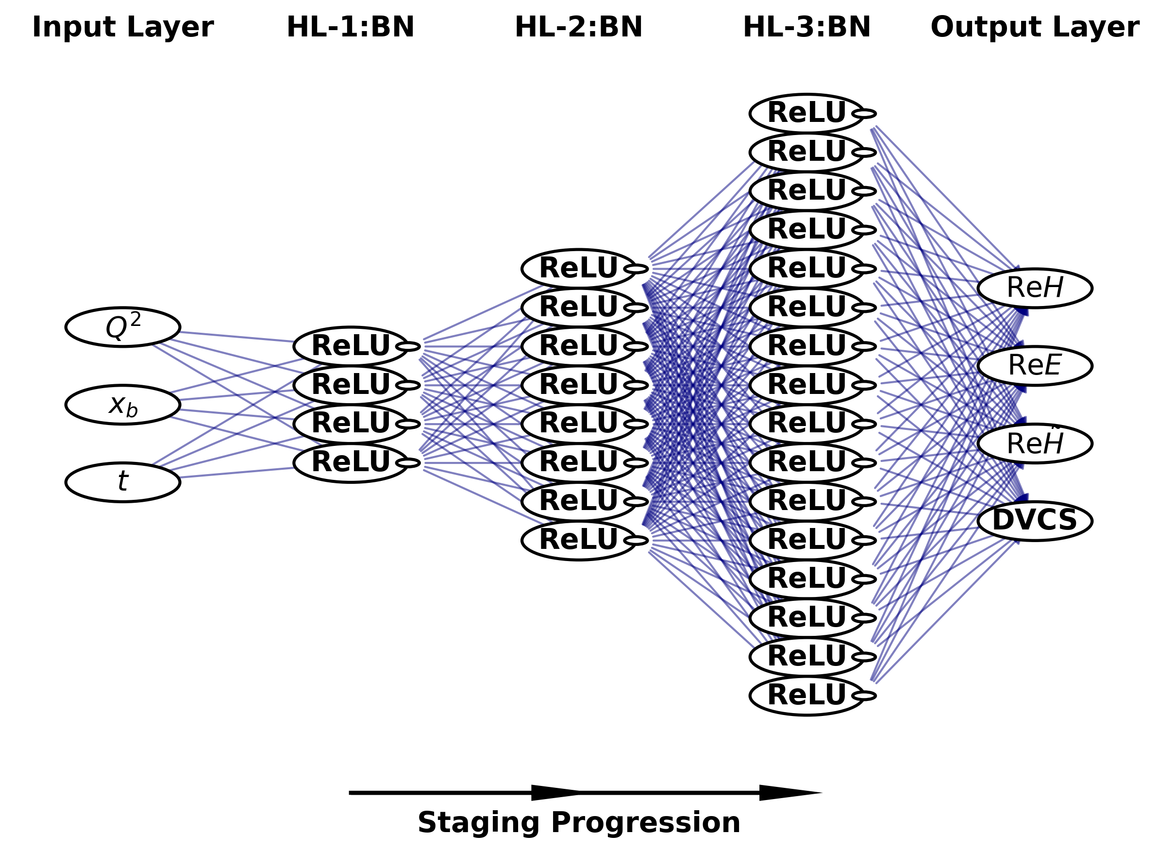
Figure 1: An example of a progressive deep neural network (DNN) architecture illustrating the staged expansion of hidden layers. The input layer consists of three variables $\mathbf{Q^{2},x_{b},t}$, feeding into progressively growing hidden layers (HLs) with ReLU activations and Batch Normalization (BN) applied at each stage. The network expands from 4 to 8 to 16 nodes per layer before reaching the output layer, which predicts the Compton Form Factors (CFFs) $ReH,ReE,\tilde{ReH},$ and DVCS amplitude. The staging progression is indicated by a directional arrow at the bottom, showing the stepwise increase in network complexity as layers grow. This example architecture is simpler than the one used in the study so that it can be scaled to diagrammatic size.

The progressive architecture allows the model to gradually adapt its weights, mitigating the effect of varying input scales. Additionally, the Adam optimizer, which adjusts learning rates dynamically based on the scale of gradient updates, further reduces sensitivity to raw input magnitudes. Weight initialization using a normal distribution with a mean of zero and a standard deviation of 0.1 ensures reasonable starting values, preventing large initial imbalances.

While feature scaling can be beneficial in cases where input variables span vastly different ranges, the controlled nature of this dataset—where kinematic variables remain consistent across training replicas—further minimizes its necessity. If input ranges varied significantly across different datasets, such as $Q^{2}$ ranging from 1 to 10, $x_{B}$ from 0 to 1, and $t$ from -1 to 0, unscaled inputs could introduce bias in early weight updates. However, in this setup, fluctuations primarily arise in the target values rather than the inputs, ensuring stability across training iterations. Explicit feature scaling is unnecessary in this progressive DNN due to the fixed nature of the training inputs, the stabilizing effects of BatchNormalization, the adaptive properties of the optimizer, and a physics-driven loss function that prioritizes output accuracy over raw input values. While feature scaling remains a useful technique in broader applications, the specific characteristics of this model ensure effective learning without the need for preprocessing input features.

After generating the pseudodata sets, a DNN model is trained for each replica to extract the parameters. For every covariance-sampled instance of the pseudodata, the model outputs a predicted parameter value (informed bootstrapping), resulting in a distribution of predictions for each CFF. The mean of this distribution reflects the accuracy of the extraction method, while the width represents the precision. These metrics are discussed in the next subsection.

3.2 Types of Contributing Errors

To comprehensively evaluate the performance of the DNN used in extraction, we employ four distinct error metrics—algorithmic error, methodological error, precision, and accuracy—to assess the reliability and robustness of the DNN outputs for a particular dataset with fixed kinematics. Each metric targets a specific aspect of the extraction process, providing a multifaceted view of the DNNs’ effectiveness in obtaining the CFFs reliably from the data containing experimental errors.

The algorithmic error quantifies the uncertainty inherent in the extraction algorithm itself, independent of any simulated experimental uncertainty in the data set. To calculate this, 1,000 identical replicas of the cross-section are generated without sampling from within the error (smearing). The resulting distribution of CFF values is analyzed, and the spread (e.g., standard deviation) of these values serves as the measure of algorithmic error. This metric isolates the limitations and intrinsic variability of the algorithm, such as numerical instabilities, approximations, or aspects of DNN initialization, offering insight into its consistency under ideal conditions.

In contrast, the methodological error captures the uncertainty arising from modeling assumptions, parameter choices and kinematic dependence embedded in the extraction process. To estimate this, controlled variations are introduced in the parameters of the CFF-generating function, producing a range of plausible parameter sets. These varied parameters are then used to generate new sets of CFFs with new sets of noisy cross-section data that replicate the spread observed in the original extracted CFFs. Subsequently, extractions are performed on the various groups of pseudodata, and the residuals—the differences between the extracted and generated CFFs—are computed. The spread of the mean in the residuals across all the various parameterizations of the generator defines the methodological error, reflecting the sensitivity of the extraction outcomes to the embedded assumptions. This process involves propagating parameter variability through the generating function to systematically assess its impact on the extracted CFFs. Minimizing methodological error requires building a model that is sensitive to the data, yet stable over small changes, relying on iterative refinement through a pseudodata generator to approximate the true CFFs present in the experimental data. This recursive approach, repeating the extraction of information and updating the generator, helps to converge on an optimal estimate of this error component, distinguishing it from purely algorithmic or statistical effects, and highlighting the systematic influence of modeling decisions.

The accuracy, defined by Equation (5), evaluates the degree to which the mean distribution of the extracted CFFs aligns with the true CFFs (from the generator), serving as a benchmark for the correctness of the results. Accuracy, $\epsilon(x_{B},t,Q^{2})$, is calculated as,

$$\epsilon(x_{B},t,Q^{2})=|CFF_{DNN}-CFF_{true}|.$$ (5)

Accuracy, as used here, is a single instance of the many tests of generator parameter variations required to quantify the uncertainty represented by the methodological error.

The value from the generating function used to produce the true CFF values are produced from the basic model using Eq. 4. From this definition, methodological error can be described as the dispersion or standard deviation of multiple accuracy measurements taken across various model parameterizations (generator variations) for fixed kinematics. Explicitly, the methodological error, $\sigma_{\text{method}}$, can be expressed as:

$$\sigma_{\text{method}}(x_{B},t,Q^{2})=$$ (6)

$$\sqrt{\frac{1}{N-1}\sum_{i=1}^{N}\left[\epsilon_{i}(x_{B},t,Q^{2})-\overline{\epsilon}(x_{B},t,Q^{2})\right]^{2}}$$

where $\epsilon_{i}(x_{B},t,Q^{2})$ is the accuracy (Eq. 5) for the $i^{th}$ realization of the varied generator parameters at fixed kinematics $(x_{B},t,Q^{2})$. $N$ is the number of realizations or parameter variations tested. $\overline{\epsilon}(x_{B},t,Q^{2})$ is the average accuracy across the $N$ realizations, given by:

$$\overline{\epsilon}(x_{B},t,Q^{2})=\frac{1}{N}\sum_{i=1}^{N}\epsilon_{i}(x_{B},t,Q^{2}).$$

More formally, ($\epsilon$) measures how close the extracted CFF (from DNN) is to the true (generated) CFF. While the methodological error ($\sigma_{\text{method}}$) quantifies how sensitive or robust the extraction method (DNN model) is against variations in the generator parameters at fixed kinematic conditions. It encapsulates the uncertainty introduced by model choices and assumptions.

The precision, calculated using Equation (7), measures the variation in the extracted CFFs in the replica distribution, indicating the consistency of the DNN outputs under repeated trials given the initial experimental uncertainty in the cross-section data. When not intentionally separated, precision will include both the algorithmic error and the propagated experimental error.

Precision, $\sigma(x_{B},t,Q^{2})$, can be expressed as:

$$\sigma(x_{B},t,Q^{2})=\sqrt{\frac{\sum_{i}\left(CFF^{i}_{DNN}-\overline{CFF}_{DNN}\right)^{2}}{N}}.$$ (7)

To accurately quantify the methodological error, one must first define a nominal mean, representing the baseline scenario for the CFF generator variation. This nominal mean should be established through first iteration of experimental data fits leading to a nominal parameter set denoted by $\vec{p}_{0}$. Thus, the true CFF values $\text{CFF}_{\text{true}}(x_{B},t,Q^{2};\vec{p}_{0})$ in the pseudodata testing should be updated from best results as accuracy and precision improve from the fits of the experimental data. Without the initial experimental data fits, the nominal means are simply asserted for DNN model testing of the pseudodata.

With this baseline established, systematic variations of the model parameters around their nominal values are introduced to explore and bound plausible deviations in the generator. Such variations can be parameterized fractionally, as $p_{i}\in[p_{i,0}(1-\delta_{i}),p_{i,0}(1+\delta_{i})]$, with $\delta_{i}$ representing fractional uncertainties (e.g., $\pm 10\%$ or $\pm 20\%$), or absolutely, as $p_{i}\in[p_{i,0}-\Delta p_{i},p_{i,0}+\Delta p_{i}]$, based on the experimental uncertainties.

The range of variation in the bounds is initially based on the precision of the CFFs. The CFF generator parameters are varied for a fixed DNN model to study the resulting deviations. However, this metric can be used to recursively improve the model until the methodological error is minimized. When performing a fit to real experimental data, its critical to recursively improve the generator to better represent the experimental CFFs, updating the nominal means, so the final systematic error can be well quantified without biased influences from theory.

Through the analysis of these four metrics: algorithmic error, methodological error, precision, and accuracy, a detailed understanding of the strengths and limitations of DNNs can be acquired for a particular experimental error condition. This approach not only isolates distinct sources of uncertainty, but also facilitates targeted improvements in the extraction process, ensuring robust and optimized results.

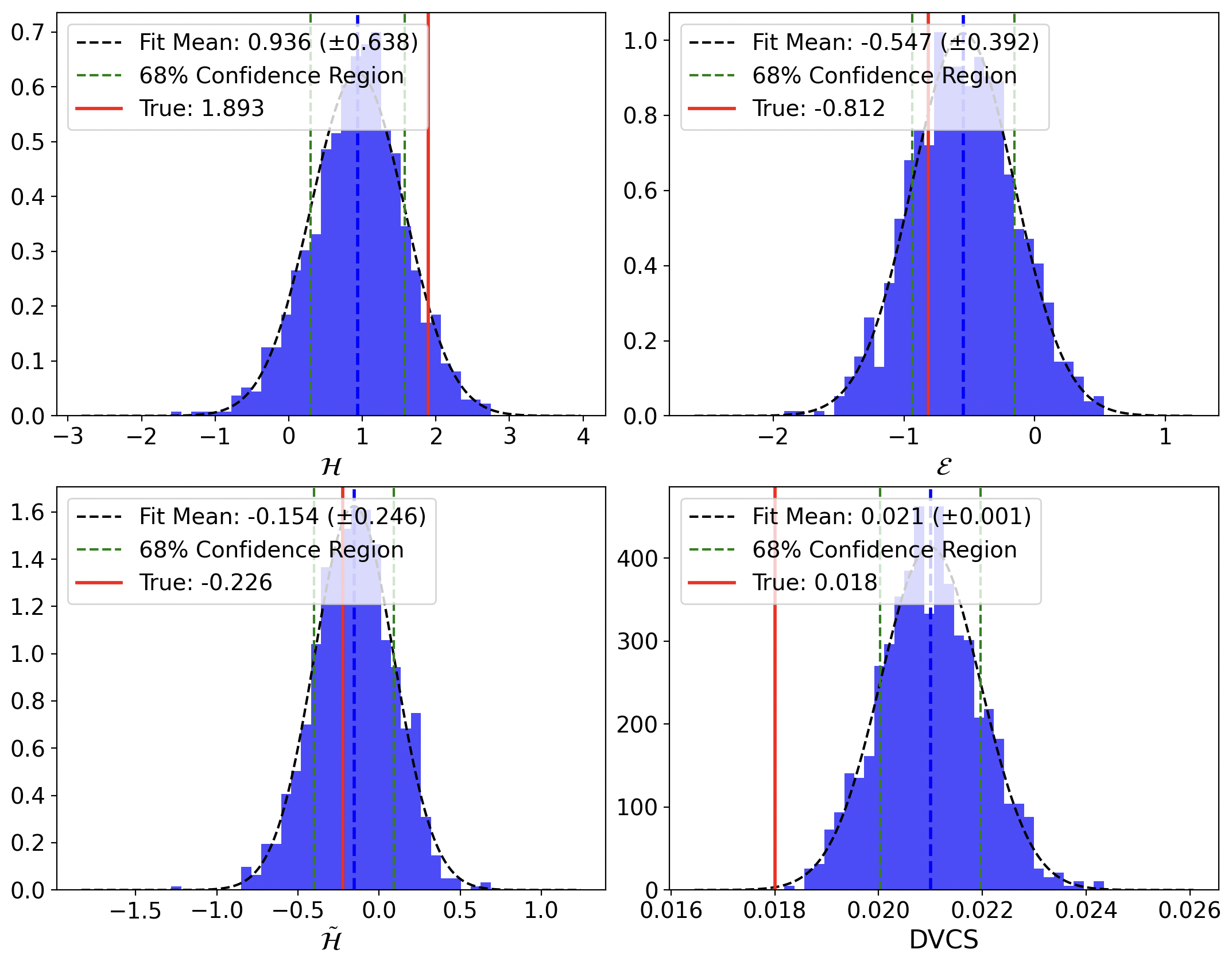
Figure 2: The CFFs and DVCS extraction using the pseudodata example demonstrating a typical fit result for the pseudodata set simulating the Hall A data for $Q^{2}=2.091$, $x_{B}=0.4$, $t=-0.371$, and $k=5.75$. In this example both $\Re e\mathcal{H}$ accuracy and precision are poor. For $\Re e\mathcal{E}$ and $\Re e\mathcal{\tilde{H}}$ the true value (red line) lies within 68% confidence level of the prediction (blue dotted line) determined by using 1000 replica models sampled from the experimental error bars. However, the distribution are quite wide with respect to the scale of the experimental error.

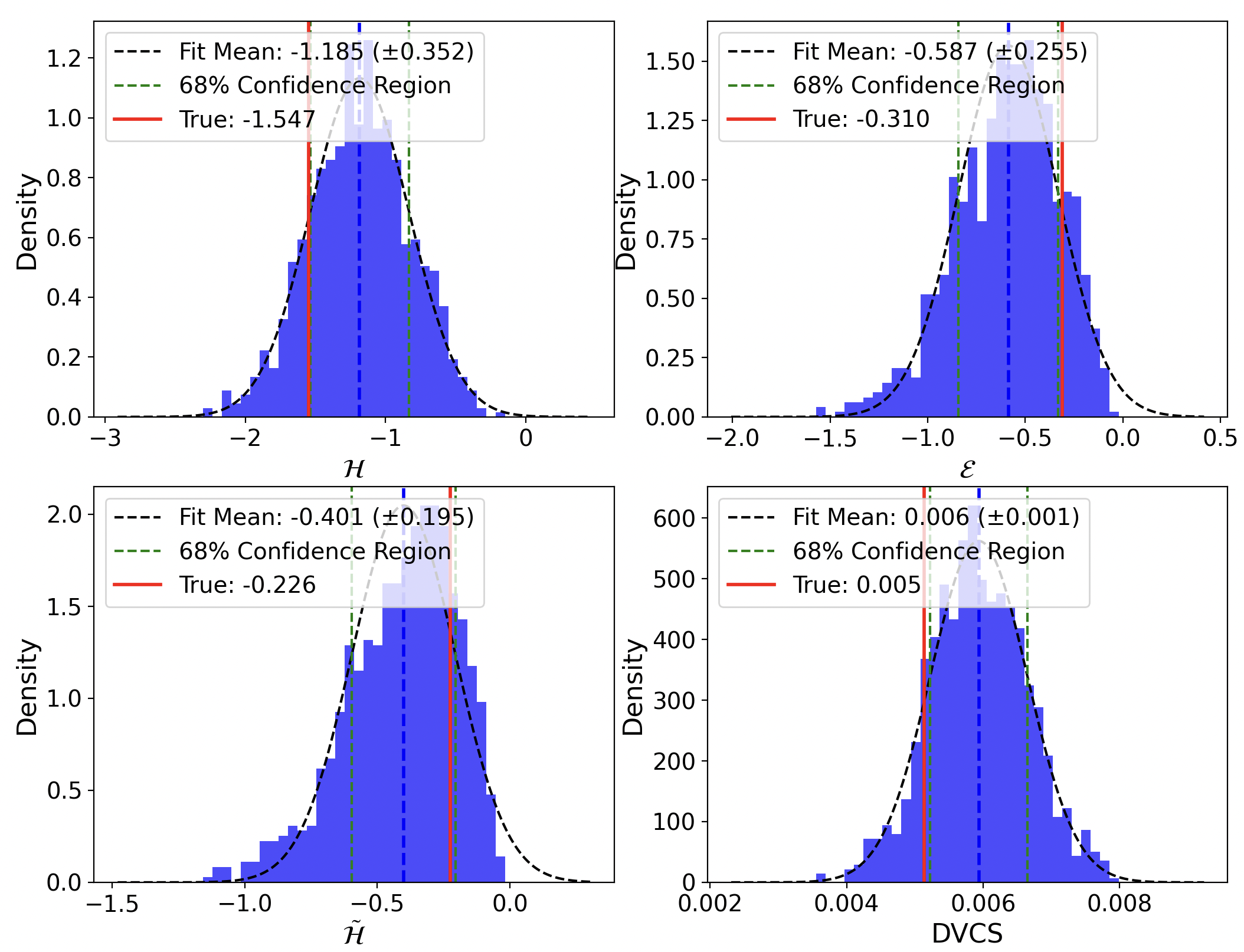
Figure 3: The CFFs and DVCS extraction using the pseudodata example demonstrating a typical fit result for the pseudodata set simulating the Hall A data for $Q^{2}=2.091$, $x_{B}=0.4$, $t=-0.371$, and $k=5.75$ but with a different CFF generator parameterization. In this example the $\Re e\mathcal{H}$ deviation of the mean and the width are within about 25% of the true. For $\Re e\mathcal{E}$ and $\Re e\mathcal{\tilde{H}}$ the true value (red line) lies within 68% confidence level of the prediction (blue dotted line) determined by using 1000 replica models sampled from the experimental error bars. However, the distribution are quite wide with respect to the scale of the experimental error.

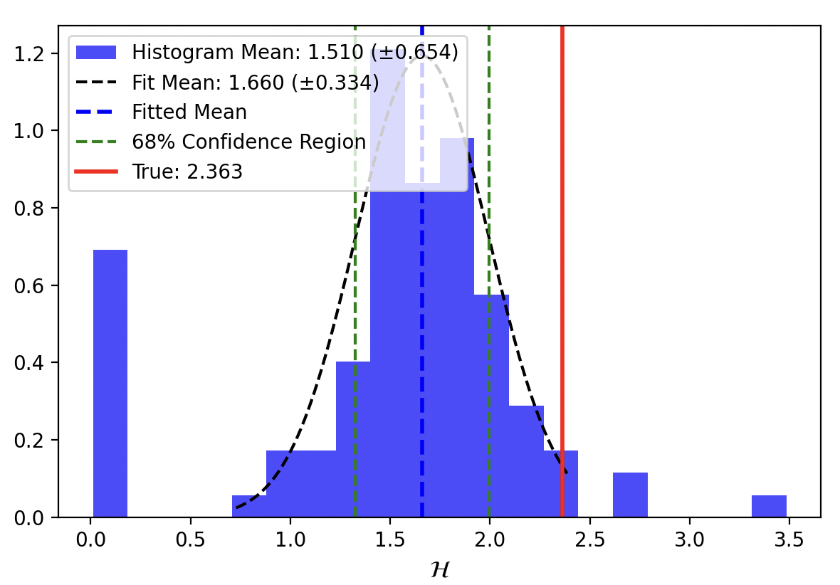
Figure 4: A demonstration of a $\Re e\mathcal{H}$ CFF extraction using the pseudodata set simulating the Hall A data for $Q^{2}=2.193$, $x_{B}=0.342$, $t=-0.371$, and $k=5.75$, showing how a DNN model can result in outliers that distort the histogram mean. In this case there are several replica models that result in zero making the mean lower than the Gaussian fit mean. Only 100 replicas are used here.

3.3 Uncertainties in the Extraction

When the experimental error sampling is applied, both statistical and systematic errors propagate from the cross sections to the CFFs. For a well-tuned model, algorithmic uncertainty should generally contribute less than 10% to the total width of the final distribution of replicas. If the algorithmic uncertainty is large, it indicates that the model is not adequately capturing the underlying data patterns or some fundamental aspect of the model is not configured appropriately (i.e., DNN initializations). The full distribution of replicas should demonstrate an accuracy and precision that are consistent with the original experimental error in the cross section. The experimental errors (systematic and statistical) generally change for each $\phi$ bin, but it is the combination of these errors for fixed kinematics that determines the scale of the propagated error to the CFFs. To estimate the overall composite error the absolute error from each point is propagated first, then the relative error is calculated from the combined result. For the JLab Hall A experimental E00-110 data sets most of the cross section data range from 15% to 35% relative error. This information can be used as a heuristic limit to determine the upper and lower bounds of the expected accuracy and precision, assuming that the extracted CFFs are of the order of 1. For CFFs close to zero, even well over 100% relative error can still pertain to a quality extraction assuming robustness of the prediction, so in these cases the standard deviation can be used to set a confidence interval in absolute terms. The approximate bound to determine if the fit is good would be $<\pm 0.35$. Fig. 2 shows the resulting fits for the three CFFs and the DVCS term from the fit result for the pseudodata set simulating the Hall A data for $Q^{2}=2.091$, $x_{B}=0.4$, $t=-0.371$, and $k=5.75$. In this example, both $\Re e\mathcal{H}$ $\epsilon$ and $\sigma$ are greater than the 35% larger limit while $\Re e\mathcal{E}$ and $\Re e\mathcal{\tilde{H}}$ are in better statistical agreement. The true value for $\Re e\mathcal{E}$ and $\Re e\mathcal{\tilde{H}}$ (red line) lies within 68% confidence level of the prediction (blue dotted line) determined by using 1000 replica models sampled from the experimental error bars. When the true value lies within the 68% confidence interval (approximately $\pm 1$ standard deviation) of the Gaussian-distributed model predictions, it indicates that the results are statistically consistent, aligning closely with normal statistical expectations. This implies there is no statistically significant bias or systematic deviation evident in the predictions, as any discrepancy observed between the model’s predicted mean and the true value falls comfortably within expected statistical fluctuations. Consequently, this situation corresponds to a p-value greater than approximately 0.32, reaffirming that the model’s uncertainties are appropriately estimated, and no statistically meaningful deviation is observed.

Figure 3 shows the resulting fits for the three CFFs and the DVCS term from the same fit result for the pseudodata set shown in Fig. 2 with $Q^{2}=2.091$, $x_{B}=0.4$, $t=-0.371$, and $k=5.75$ but with a different variation in the generator parameters. When automated to produce many such variations, $a$, and $b$ and $f$ are sampled using the mean values in Table 1 using a normal distribution with the width defined using the methodological error bounds. For this example in Fig 3 a set of distinct CFFs from the true values used in Fig. 2 are chosen. As indicated in the figure, all resulting CFFs distribution widths are within the expected upper limit and the means all are barely within the 68% confidence level. Many variations of the CFFs at fixed kinematics are produced then extracted in this way to determine the final methodological error from Eq. 6.

For the situation where the resulting model distributions are not Gaussian the histogram mean and standard deviation can be used. In some cases with just a few non-Gaussian outliers the Gaussian fit can be used to negate their impact. Figure 4 shows a pseudodata extraction for CFF $\Re e\mathcal{H}$ demonstrating a collection of poor models in the distribution accumulating around zero. When the experimental errors and the resulting CFF distributions are both approximately Gaussian then obtaining the 68% confidence level is trivial. If this is not the case then its not possible to rely on a Gaussian fit or the standard deviations to define confidence intervals directly. Instead, one would typically use methods based on percentiles, likelihood ratios, or numerical approaches.

In the statistical analysis of the model tuning and prototyping one should expect that the width of the distribution should be comparable to the known experimental uncertainties (such that algorithmic in not dominant). This means that the spread in the predictions should reflect the variability expected due to the inherent noise and uncertainty in the data. The distribution should be centered around the true parameter values with minimal bias. If there is a significant bias (a shift in the mean away from the true value), it suggests model inaccuracies or systematic errors in the extraction process. The process of model adjustment and testing would iterate until most of the true values are within the 68% confidence level with an overall model distribution width minimized to within bound define by the composite experimental error.

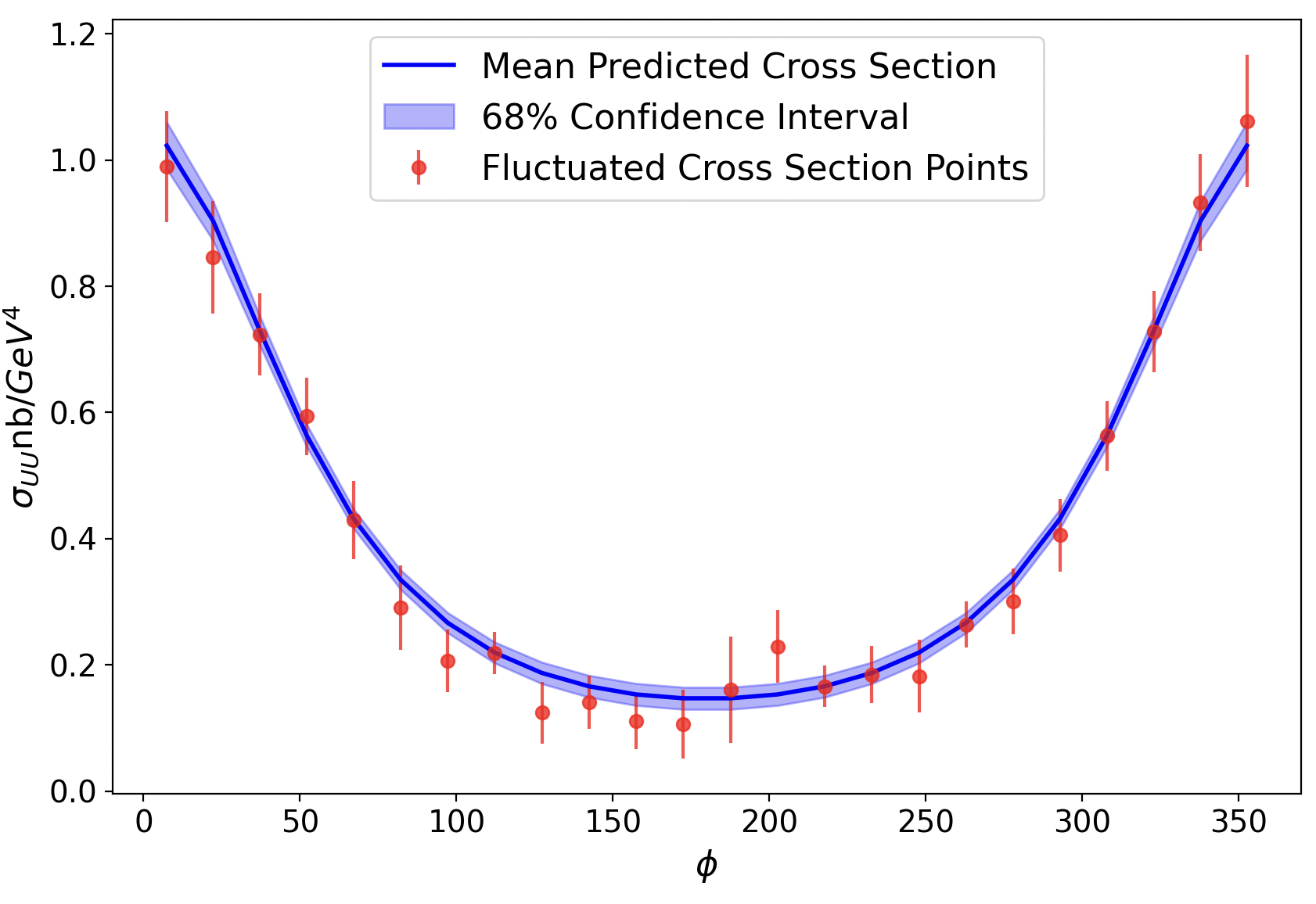
Figure 5: An example of the local fit result from pseudodata: cross-section fit represented by the solid line surrounded by light-colored error bands correspond to the 68% confidence level.

Using the ensemble of models of all of the CFFs defined in the framework along with the constant DVCS term, it is possible to plot the 68% confidence level band of predicted cross section in comparison to the original data used. Figure 5 shows this for the pseudodata extraction example. These types of picture are not particularly useful in the analysis as there are a large number of fit parameter combinations that would look equally reasonable. This issue is technically referred to as parameter degeneracy or nonidentifiability. In complicated fit functions with multiple parameters, it can be challenging to converge on a unique set of parameter values because different combinations of parameters can result in similarly good fits to the data. Another common issue is parameter correlation, where the CFFs are highly correlated, and changes in one parameter can be compensated for by changes in another, leading to multiple valid solutions. Best practices entail focusing on the direct extraction of the CFFs understanding in detail the accuracy and precision of the model result for each CFF and their correlations by varying the true values in pseudodata generation process and iterating the full extraction several times proving model stability and reliability for a realistic range of true values. Additional useful tools in this phase of the analysis and systematic studies are methods such as regularization Bayesian inference. These approaches help constrain the parameter space and reduce the likelihood of degeneracy, improving the reliability of the parameter extraction process.

The methodological error is estimated by changing the CFF generator for the same kinematics and going through the same extraction process over again with just slightly different CFFs. To perform this study, the generator model parameters in Table 1 are varied so that the CFFs change within the initial widths of the model distribution shown in Figures 1-3. This process is done enough times to produce a residuals distribution for each CFF, which is determined by the difference between the distribution of model means and the changing true values. In this test case, the process was repeated 200 times, but for a much better measure of the methodological error, the same number of trials is required as the number of models used ($\sim 1000$).

Table 2: The absolute error estimates from each contributing category: Algo. (algorithmic error), Meth. (Methodological error), Gaus. (distribution mean from the Gaussian fit), Hist. (Histogram mean), and Acc. (accuracy).

$CFFs$	Algo.	Meth.	Gaus.	Histo.	Acc.
$\Re e\mathcal{H}$	0.03	0.73	0.320	0.645	0.611
$\Re e\mathcal{E}$	0.02	0.10	0.178	0.310	0.05
$\Re e\widetilde{\mathcal{H}}$	0.10	0.10	0.144	0.143	0.01
$DVCS$	0.0001	0.005	0.050	0.057	0.002

Table 2 summarize the analysis for the pseudodata set simulating the Hall A data for $Q^{2}=2.091$, $x_{B}=0.4$, $t=-0.371$, and $k=5.75$ . The table shows the resulting error estimates form the pseudodata uncertainty analysis in the category of algorithmic error, methodological error (accuracy over variation), the width of the Gaussian (precision), and the histogram distribution. Accuracy is also listed for the initial instance of the extraction prior to generator variations.

3.4 Optimal Data Access

The analysis in the previous section relies on data from a previously published Hall A collaboration paper, with uncertainty estimates directly taken from that publication. Consequently, these estimates are limited, as no detailed experimental covariance matrix is available. To enable a more thorough analysis, access to the original experimental data with a covariance matrix, along with unbinned cross-section data spanning the experiment’s kinematic range, would be crucial. In the absence of this information, the current binning configuration is fixed, and the generated training data is also restricted to this binned format.

This limitation hinders the ability to analyze how the observable varies with respect to $\phi$ and to assess the error correlations $\delta\phi$ across these variations. The resolution of $\phi$ binning, the number and size of bins, and general bin migration effects become critical factors for optimal information extraction. Similarly, variations in the mean kinematic values of $x_{b}$, $t$, and $Q^{2}$ could significantly enhance the extraction of the CFFs using the same experimental data.

Most importantly, the lack of access to the data details restricts the ability to perform systematic resampling, which is essential for fully utilizing AI-based extraction methods. Future work will address the specifics of the methodology under conditions of optimal data access. It is critical to note that this is the common limitation in which most local and ultimately global analyses are performed, which speaks to the loss of essential experimental information as a standard.

To rigorously evaluate the proposed method for extracting CFFs from experimental data, a systematic and controlled testing framework is essential. Traditionally, CFFs are extracted by binning experimental data in kinematic variables such as $Q^{2}$, $t$, $x_{b}$, and $\phi$, and then fitting theoretical models to these discrete bins to match the observed cross-sections. However, this fixed-bin approach imposes limitations on resolution and may not fully exploit the kinematic sensitivity inherent in the data, as the predefined bins might not align with regions where the CFFs exhibit significant variation. The proposed method addresses these challenges by employing a DNN to model the CFFs directly as continuous functions of the kinematic variables $Q^{2}$, $t$, and $x_{b}$. This approach can provide more information to perform a better local fit at fixed kinematics but also holds the potential to better connecting the kinematics in a single model more similar to a global fit.

The testing framework relies on an event generator that produces synthetic DVCS events mimicking the statistical properties of experimental data. This generator employs Monte Carlo techniques to create pseudo cross-section data based on theoretical cross-sections computed from known CFFs, which serve as the ground truth for validation. By incorporating statistical fluctuations and experimental uncertainties, the synthetic data replicate the challenges of real measurements. The use of predefined CFFs ensures that the true values are known, providing a clear standard for evaluating the extraction method’s performance. The use of the event generator provides the means for recursive re-binning and kinematic resampling while providing the utility to more realistically simulate various experimental errors in a multivariate schema.

This DNN-based method with recursive re-binning offers significant advantages over traditional fixed-bin approaches. The flexibility to evaluate CFFs at any kinematic point allows for a dynamic sampling strategy, where the effective ”binning” can be adjusted to create a fine-grained representation in regions of rapid CFF variation—such as near specific $t$-values where certain GPD contributions peak—or in sparse data zones, without being bound by predetermined bin edges. By learning a smooth, continuous function, the DNN interpolates between data points, mitigating the statistical noise that often affects bin-by-bin fits and providing a more robust estimate in regions with limited measurements by drawing on information from nearby kinematics. The global optimization during training captures correlations across the entire kinematic space, yielding a consistent model that reflects the interconnected nature of the CFFs, unlike fixed-bin methods that treat each bin independently. The recursive re-binning enhances kinematic sensitivity by concentrating evaluation points in areas where specific CFFs dominate or where the data are most informative, enabling a targeted exploration of the phase space. In sparse regions, the DNN’s ability to generalize from neighboring kinematics reduces uncertainties that would plague empty or poorly populated bins in traditional methods. In the next section, a simple case using this methodology is explored.

3.5 Uncertainty Minimization in DNN Extraction

Any local fitting method of extracting CFF from fixed kinematic cross sections is fundamentally limited. The cross section values presented in published data does not generally provide enough information to fully leverage the power of DNNs for optimal information extraction. With just a small amount of additional information that exists in the experimental data, the appropriate DNN approach can significantly enhance the extraction process far beyond what traditional local DNN fits are capable of. There are two critical aspects of experimental information that make this approach outperform. One is a detailed experimental covariance matrix. The other is the capacity to perform kinematic resampling and re-binning of the data.

To construct an experimental covariance matrix representing the detector resolutions for sampling in the DNN extraction, we again use the experiment E00-110 at JLab’s Hall A as an example. To account for the uncertainties and correlations in the kinematic variables influenced by the detectors, information is required about the scattered electron, detected in the High-Resolution Spectrometer (HRS), the emitted photon (detected in the electromagnetic calorimeter), and the recoil proton (detected in the Proton Array) data . The key kinematic variables are $x_{B}$, $Q^{2}$, $t$, and $\phi$, determined from the electron kinematics, virtual photon direction, and detected photon direction, with additional constraints from the exclusivity cuts.

The covariance matrix will describe the uncertainties in the measured quantities—momentum and angles—and their correlations, based on the detector resolutions and geometric acceptances provided. Since the variables $x_{B}$, $Q^{2}$, $t$, and $\phi$ are derived from primary measurements (e.g., electron momentum $p$, scattering angles, photon angles, and energy), we’ll first define the resolution and acceptance effects on these primary quantities and then propagate them to the kinematic variables if needed. After the 4-vectors are produced from the event generator the conversion to detector variables is performed so the Monte Carlo sampling will directly use the detector-level variables, and the final sampled events will obtain the experimental uncertainties in the covariance matrix.

First, it is necessary to identify key variables and resolutions from the experimental configuration. In the case of the scattered electron (HRS) there is a momentum resolution of $\delta p/p=2\cdot 10^{-4}$ (relative uncertainty) and an angular resolution (horizontal plane): $\delta\theta_{e}=2\,\text{mrad}$ with slightly worse vertical angular resolution, $\delta\phi_{e}=2\,\text{mrad}$ unless otherwise constrained. The acceptance is $6\,\text{msr}$ solid angle, and $\pm 4.5\%$ in momentum data .

For the case of the emitted photon (calorimeter) there is an angular resolution in the calorimeter which covers $\sim 0.1\,\text{sr}$ with a front face at 1.1 m. The resolution depends on the granularity (block size). Half a block shift suggests a block size of order $\sim 5-10\,\text{cm}$ (typical for such calorimeters), yielding an angular resolution of $\delta\theta_{\gamma}\approx 5-10\,\text{cm}/1.1\,\text{m}\approx 5-9\,\text{mrad}$. Here we use $7\,\text{mrad}$ as a reasonable estimate. Two angles are measured relative to the virtual photon direction ($\theta_{\gamma}$, $\phi_{\gamma}$), so assume similar resolution for both. For energy resolution the electromagnetic calorimeters has approximately $\delta E/E\approx 5\%/\sqrt{E(\text{GeV})}$; this affects the exclusivity cut but not directly $t$ or $\phi$ data .

For the case of the recoil proton (Proton Array) the angular resolution of the 100 blocks in a C-ring configuration over $\sim 2\pi$ in $\phi$ suggest $\delta\phi_{p}\approx 2\pi/100\approx 63\,\text{mrad}$. Radial resolution depends on block size, assume $\delta\theta_{p}\approx 50\,\text{mrad}$ (coarser than HRS or calorimeter). This would normally be used for exclusivity crosschecks, so its resolution may not directly enter the primary covariance matrix unless explicitly required.

The kinematic variables and corresponding bin structure depend on the relationship to these resolution terms. For example, $x_{B}$ and $Q^{2}$ depend on electron momentum and angles. $t$ and $\phi$ depend on the virtual photon direction (from electron) and detected photon direction. The covariance matrix is constructed using the primary measured quantities: electron momentum $p$, electron angles $\theta_{e}$ and $\phi_{e}$, and photon angles $\theta_{\gamma}$ and $\phi_{\gamma}$. These are the variables directly affected by detector resolutions, and their uncertainties propagate to $x_{B}$, $Q^{2}$, $t$, and $\phi$. The proton variables are not included in this example, assuming the exclusivity cut is applied post-sampling.

The vector of variables are $\vec{x}=(p,\theta_{e},\phi_{e},\theta_{\gamma},\phi_{\gamma})$, and the covariance matrix $V$ is a 5 by 5 symmetric matrix where diagonal elements are variances ($\sigma_{i}^{2}$) and off-diagonal elements are covariances ($\sigma_{ij}$):

$$V=\begin{pmatrix}\sigma_{p}^{2}&\sigma_{p,\theta_{e}}&\sigma_{p,\phi_{e}}&\sigma_{p,\theta_{\gamma}}&\sigma_{p,\phi_{\gamma}}\\ \sigma_{p,\theta_{e}}&\sigma_{\theta_{e}}^{2}&\sigma_{\theta_{e},\phi_{e}}&\sigma_{\theta_{e},\theta_{\gamma}}&\sigma_{\theta_{e},\phi_{\gamma}}\\ \sigma_{p,\phi_{e}}&\sigma_{\theta_{e},\phi_{e}}&\sigma_{\phi_{e}}^{2}&\sigma_{\phi_{e},\theta_{\gamma}}&\sigma_{\phi_{e},\phi_{\gamma}}\\ \sigma_{p,\theta_{\gamma}}&\sigma_{\theta_{e},\theta_{\gamma}}&\sigma_{\phi_{e},\theta_{\gamma}}&\sigma_{\theta_{\gamma}}^{2}&\sigma_{\theta_{\gamma},\phi_{\gamma}}\\ \sigma_{p,\phi_{\gamma}}&\sigma_{\theta_{e},\phi_{\gamma}}&\sigma_{\phi_{e},\phi_{\gamma}}&\sigma_{\theta_{\gamma},\phi_{\gamma}}&\sigma_{\phi_{\gamma}}^{2}\end{pmatrix}$$ (8)

The diagonal elements (variances) can be quantified as $\sigma_{p}^{2}=(p\cdot\delta p/p)^{2}=(p\cdot 2\cdot 10^{-4})^{2}$, where $p$ is the nominal momentum (e.g., beam energy  1-6 GeV). Then $\sigma_{\theta_{e}}^{2}=(2\cdot 10^{-3})^{2}=4\cdot 10^{-6}\,\text{rad}^{2}$ and $\sigma_{\phi_{e}}^{2}=(2\cdot 10^{-3})^{2}=4\cdot 10^{-6}\,\text{rad}^{2}$, with $\sigma_{\theta_{\gamma}}^{2}=(7\cdot 10^{-3})^{2}=49\cdot 10^{-6}\,\text{rad}^{2}$. and $\sigma_{\phi_{\gamma}}^{2}=(7\cdot 10^{-3})^{2}=49\cdot 10^{-6}\,\text{rad}^{2}$.

The off-diagonal elements (covariances) for the electron variables ($p$, $\theta_{e}$, $\phi_{e}$) from the HRS momentum and angles will normally have small correlations due to optics, but these are typically weak ($<10\%$) however it is still advantageous to include this information if a detailed transport matrices are available.

Photon variables ($\theta_{\gamma}$, $\phi_{\gamma}$) from the calorimeter block geometry might introduce correlation if a photon hits near a block edge, but with coarse resolution and symmetry, assume negligible correlation. Also, the electron-photon correlations should generally be zero since the virtual photon direction depends on electron kinematics and the detected photon is independent.

The kinematic variables $x_{B}$, $Q^{2}$, $t$, and $\phi$ are derived from the primary measured quantities (electron momentum $p$, electron angles $\theta_{e}$ and $\phi_{e}$, and photon angles $\theta_{\gamma}$ and $\phi_{\gamma}$), which are subject to the detector resolutions, uncertainties and correlations encoded in the covariance matrix. The binning of these kinematic variables—i.e., how events are grouped into discrete intervals in $x_{B}$, $Q^{2}$, $t$, and $\phi$—depends on the uncertainties and correlations in these primary measurements.

For the kinematic variable definitions $x_{B}$ is defined by $x_{B}=\frac{Q^{2}}{2M_{p}\nu}$, where $Q^{2}$ is the virtual photon four-momentum squared, $\nu=E-E^{\prime}$ is the energy transfer ($E$ is the beam energy, $E^{\prime}$ is the scattered electron energy), and $M_{p}$ is the proton mass. $E^{\prime}=p$ (assuming ultrarelativistic electrons), and $Q^{2}=4EE^{\prime}\sin^{2}(\theta_{e}/2)$, so $x_{B}$ depends on $p$ and $\theta_{e}$. $Q^{2}$ (four-momentum transfer squared) is defined as $Q^{2}=4EE^{\prime}\sin^{2}(\theta_{e}/2)$ and is directly tied to $p$ (since $E^{\prime}=p$) and $\theta_{e}$. The $t$ (mandelstam variable) is defined as $t=(q-p_{\gamma})^{2}$, where $q$ is the virtual photon four-momentum ($q=k-k^{\prime}$, with $k=(E,\vec{k})$ the beam and $k^{\prime}=(E^{\prime},\vec{k}^{\prime})$ the scattered electron), and $p_{\gamma}$ is the emitted photon four-momentum. The virtuality $q$ depends on $p$, $\theta_{e}$, and $\phi_{e}$ (via electron kinematics); $p_{\gamma}$ depends on photon energy $E_{\gamma}$ and angles $\theta_{\gamma}$, $\phi_{\gamma}$ relative to $q$.

The azimuthal angle $\phi$ is defined by the angle between the electron scattering plane (defined by $\vec{k}$ and $\vec{k}^{\prime}$) and the photon production plane (defined by $\vec{q}$ and $\vec{p}_{\gamma}$). This is determined by $\phi_{e}$ (electron azimuthal angle) and $\phi_{\gamma}$ (photon azimuthal angle) relative to the virtual photon direction.

The covariance matrix $V$ describes the uncertainties in $(p,\theta_{e},\phi_{e},\theta_{\gamma},\phi_{\gamma})$. These uncertainties propagate to $x_{B}$, $Q^{2}$, $t$, and $\phi$ via their functional dependencies. The bin sizes must be chosen larger than the resolution-induced smearing to ensure statistical significance and avoid over-resolving the data beyond experimental precision. Using error propagation (first-order Taylor expansion), the variance of a derived quantity $f(p,\theta_{e},\dots)$ is:

$$\sigma_{f}^{2}=\sum_{i}\left(\frac{\partial f}{\partial x_{i}}\right)^{2}\sigma_{x_{i}}^{2}+\sum_{i\neq j}\frac{\partial f}{\partial x_{i}}\frac{\partial f}{\partial x_{j}}\sigma_{x_{i}x_{j}}$$

Since $V$ is diagonal (no correlations), the cross terms vanish.

Considering $Q^{2}$ resolution, $Q^{2}=4Ep\sin^{2}(\theta_{e}/2)$, and $\frac{\partial Q^{2}}{\partial p}=4E\sin^{2}(\theta_{e}/2)$,with

$$\frac{\partial Q^{2}}{\partial\theta_{e}}=4Ep\sin(\theta_{e}/2)\cos(\theta_{e}/2)=2Ep\sin\theta_{e},$$

and $\sigma_{Q^{2}}^{2}=\left(4E\sin^{2}(\theta_{e}/2)\right)^{2}\sigma_{p}^{2}+\left(2Ep\sin\theta_{e}\right)^{2}\sigma_{\theta_{e}}^{2}$.

For $x_{B}$ resolution, $x_{B}=\frac{Q^{2}}{2M_{p}(E-p)}$, $M_{p}=0.938\,\text{GeV}$, where $\sigma_{x_{B}}$ depends on $\sigma_{Q^{2}}$ and $p$, but $\nu=E-p$ dominates the denominator sensitivity.

For $t$ resolution, $t$ depends on the angle between $\vec{q}$ and $\vec{p}_{\gamma}$, sensitive to $\theta_{e}$, $\phi_{e}$, $\theta_{\gamma}$, and $\phi_{\gamma}$. For small angles, $t\approx-q^{2}-p_{\gamma}^{2}+2|q||p_{\gamma}|\cos\theta_{q\gamma}$, with $\sigma_{t}$ is dominated by $\sigma_{\theta_{\gamma}}$ (7 mrad) since HRS resolution is finer. Typical $\sigma_{t}\approx 0.01-0.05\,\text{GeV}^{2}$, depending on kinematics.

Additionally, this information should be considered for the dependence on binning. For the example analysis, if the bin sizes in $x_{B}$, $Q^{2}$, $t$, and $\phi$ should be minimized beyond the scale set by the resolutions with bins smaller than $\sigma$ this would lead to noise-dominated distributions ($\Delta Q^{2}\gtrsim 0.01\,\text{GeV}^{2}$, $\Delta x_{B}\gtrsim 0.01$, $\Delta t\gtrsim 0.05\,\text{GeV}^{2}$, $\Delta\phi\gtrsim 1^{\circ}$ (or $\sim 20\,\text{mrad}$)).

To demonstrate how to use this information in DNN fits we have to employ the event generator to produce enough statistics to demonstrate the procedure. The simulation should nominally replicate the event counts of the experimental bins being modeled, consistent with the data’s statistical errors. For this example, a few thousand events are used. An event generator produces DVCS events,

$$e(k)+p(P)\xrightarrow{\gamma^{*}(q)}e^{\prime}(k^{\prime})+p^{\prime}(P^{\prime})+\gamma(q^{\prime}),$$

using the cross section distributions with the same basic CFF generator previous discussed. For the event generator, a phase-space generator is developed to sample from the theoretical cross section to produce DVCS events with smeared 4-vectors. The smearing process samples each 4-vector variables from the covariance matrix just defined. The data can then be binned and the cross section values analyzed as previously described to obtain a DNN extraction.

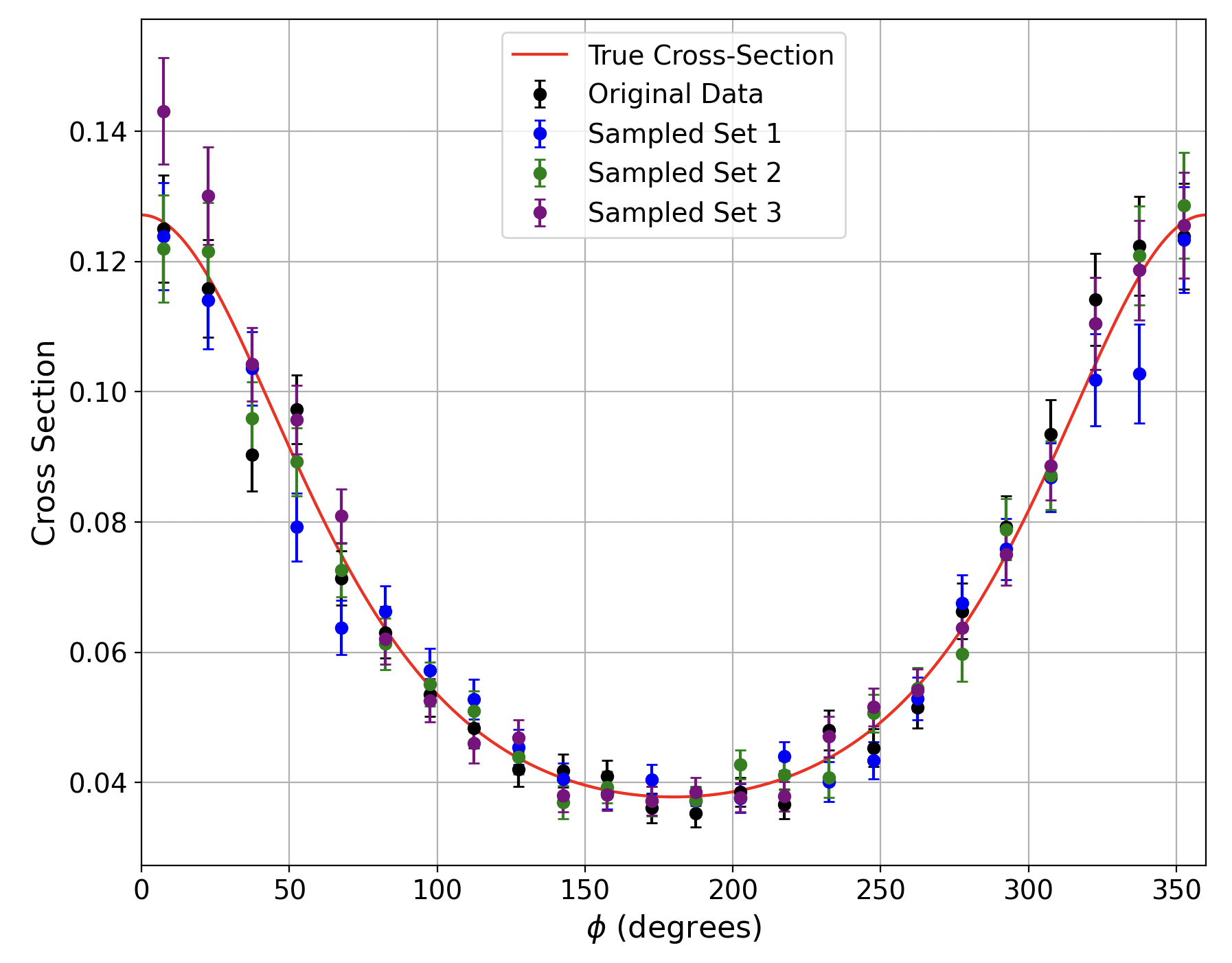
Figure 6: An example of data resampling from simulated experimental data using an event generator. In this case there are three data sampling iterations with the same mean of each kinematic bin in $t$ and $x_{b}$ but with 5% variation in the kinematic bin width for each iteration.

For simplicity, the kinematics can remain fixed and $\phi$ can be resampled multiple times to obtain more information from the data so that the AI extraction tools can be optimally leveraged to take full advantage of the information in a particular chunk of the data. The re-binning strategy and re-sampling process is critical to this approach. For example, resampling at the same fixed $\phi$ bins with slightly different bin widths in $t$ and $x_{b}$ provides a better sampling space for bootstrapping and Monte Carlo sampling for those same $\phi$ bins, see Fig. 6. To do this, the same kinematic means in $t$ and $x_{b}$ are achieved by changing the data bin widths for each in a range of 5% (based on resolution criteria) or less to the left or right to obtain fluctuations in the counts for all $\phi$ bins. Additionally, fixed kinematic bin resampling in $\phi$ in a non-overlapping domain, see Fig 7, can be achieved by shifting the starting point in $\phi$ to obtain multiple instances of bin migrations for each $\phi$ bin.

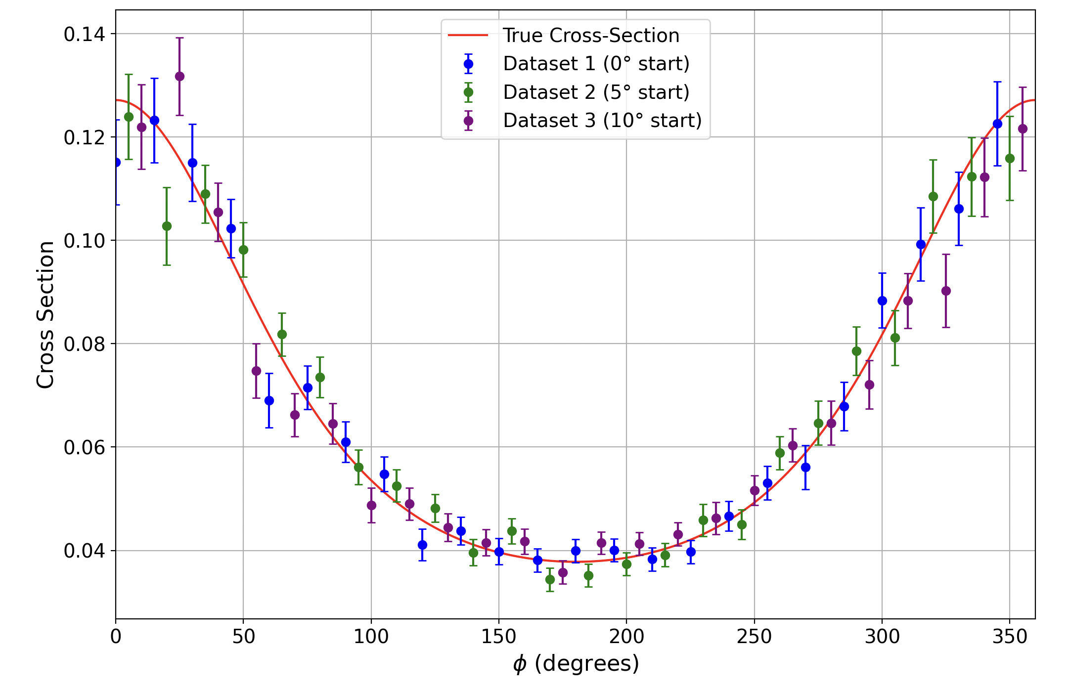
Figure 7: An example of data resampling from simulated experimental data using an event generator. In this case there are three data sampling iterations within the same kinematic bins but with different starting points in $\phi$ to obtain variation in bin content with the same data.

When these two schema for data resampling are combined significantly more information from the data can be obtained and much better replica generation can be achieved. In Fig. 6 and Fig. 7 only three resampling iterations are shown. This process should be systematically increased to maximize information extraction.

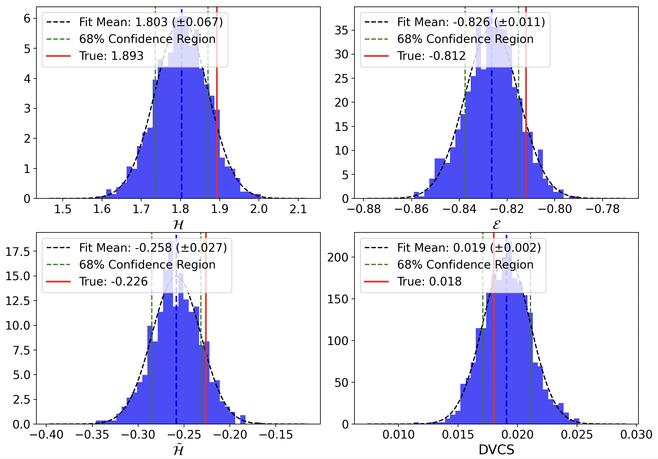
Figure 8: The CFFs and DVCS extraction using the same exact pseudodata example shown in Fig. 2 for the Hall A data for $Q^{2}=2.091$, $x_{B}=0.4$, $t=-0.371$, and $k=5.75$. The same exact model and training process was used. Only the resampling and recursive re-binning as described in the text have change leading to clear improvement in both accuracy and precision.

For each of the alternative bin configurations (both those with varied widths in $t$, $x_{b}$ and those shifted in $\phi$), performing bootstrap resampling can again be used to propagate the experimental error. Specifically, randomly sample the experimental data points from the original dataset within the experimental covariance matrix to produce numerous bootstrap replicas. For each replica, calculate the bin statistics (counts, cross sections, asymmetries, etc.) according to the chosen binning variant. Repeat this step multiple times (1000 in this case) for each bin configuration, generating a robust bootstrap distribution of each bin statistic for more extensive training. These distributions directly reflect the statistical fluctuations and provide the means to fully assess the uncertainties and correlations. An example is shown in Fig. 8 using this approach. The CFFs and DVCS extraction using the same exact pseudodata example shown in Fig. 2 for the Hall A data was used for $Q^{2}=2.091$, $x_{B}=0.4$, $t=-0.371$, and $k=5.75$. The same exact model and training process was used so that it is evident where the improvement comes from. Only the resampling and recursive re-binning as described have changed leading to significant improvement in both accuracy and precision as compared to the original fit.

The following describes the updated data generation and training scheme step by step.

1. Generate Truth CFFs: Begin with fixed kinematic values ($x_{b}$, $Q^{2}$, $t$) and generate the three CFFs and DVCS term using the basic model (e.g., Eq. (4)). Compute corresponding cross sections using the BKM10 formalism. These CFFs serve as the reference for testing.

2. Simulate Event-level Pseudodata: Create DVCS/BH like events to use as event-level pseudodata by smearing the generated four-vectors according to the experimental covariance matrix $V$ (Eq. 8), sampling from a multivariate Gaussian to reflect realistic measurement uncertainty.

3. Resample and Re-bin: Organize the event-level pseudodata into kinematic bins and apply two key resampling strategies:

   • Bin Width Variation: Slightly shift $t$ and $x_{b}$ bin widths ($\leq 5$%) to create multiple versions of the same $\phi$-bin dataset while keeping the kinematic mean fixed. This enhances statistical variation for bootstrapping.

   • Non-Overlapping $\phi$-Bin Shifts: Generate alternate $\phi$-bin sets by shifting bin boundaries. This provides independent samples with controlled bin migration.

4. Generate Replica Datasets: Using the same covariance matrix as Step 2, perform Cholesky decomposition to create a large ensemble of fluctuated replicas:

   $$F^{\text{replica}}=F+Lz,$$

   where $F$ is the pseudodata from Step 2, and $z$ is a vector of standard normal random variables. Each replica represents a statistically valid realization of an experimentally measured DVCS/BH physics process. Here, the variation is done at the event level and re-binned for analysis.

5. Train DNN on Each Replica: Train the DNN to extract the CFFs from each replica. The loss function is a weighted mean squared error using $V_{ij}$ to incorporate correlated experimental uncertainties.

6. Extract Parameter Distributions: From the ensemble of trained models, compute the distribution of extracted CFFs. The mean gives the central extracted value; the standard deviation quantifies uncertainty.

7. Analyze Uncertainty Sources: Quantify total uncertainty in the extracted CFFs, separated into Algorithmic Error, Precision, Accuracy and Methodological Error.

In the real-world application of this approach, we would then compare the extracted CFFs and update the model with the CFFs determined by the data. This would normally be done many times until the generator is a high-fidelity representation of the experimental data to within statistical errors.

In the described method, it is essential to distinguish between the purpose of generating pseudodata in Step 2 and the generation of replicas in Step 4. The smearing process in Step 2 uses the experimental covariance matrix to produce a single pseudodata set that mimics the measurement process of a real experiment. This synthetic dataset serves as a stand-in for what an actual experiment would yield, incorporating realistic experimental uncertainties through multivariate Gaussian sampling. However, this step represents only one possible outcome of an experiment and, by itself, does not provide a means to quantify the uncertainty on extracted physical observables.

In contrast, the replica generation procedure in Step 4 uses the same covariance matrix to produce an ensemble of statistically consistent realizations of the same experimental dataset. Each replica is created by adding fluctuations drawn from the covariance structure via Cholesky decomposition, thereby modeling how the measured values could have varied due to inherent experimental uncertainty. Training the DNN on each of these replicas allows one to propagate the experimental uncertainty through the model. The resulting distribution of extracted parameters provides a rigorous statistical estimate of the uncertainty, where the mean gives the central value and the spread captures the propagated error.

The technique used in this extraction constitutes a fully optimized unbinned fit at the event level, which naturally improves statistical precision relative to local binned extractions. The central aspect of this improvement stems from the fact that unbinned methods preserve the full information content of the data, avoiding the information loss associated with grouping events. As such, this event-level DNN-based extraction achieves statistical efficiency approaching the Cramér–Rao bound cramer1946 ; rao1945 , the theoretical limit on the precision of unbiased estimators.

To elaborate, consider a parameter $\theta$ estimated from a dataset $\{x_{i}\}_{i=1}^{N}$. The Cramér–Rao bound provides a lower bound on the variance of any unbiased estimator $\hat{\theta}$, given by:

$$\mathrm{Var}(\hat{\theta})\geq\frac{1}{I(\theta)},$$

where $I(\theta)$ denotes the Fisher information, defined in the unbinned case as:

$$I(\theta)=\mathbb{E}\left[\left(\frac{\partial}{\partial\theta}\log f(x;\theta)\right)^{2}\right],$$

with $f(x;\theta)$ the probability density function for the observable $x$.

In this approach, the full dataset $\{x_{i}\}$ is used without discretization. Each event contributes directly to the construction of the DNN model, which is accessed in the training process during the recursive re-binning and re-sampling. This ensures that no statistical information is discarded and the full Fisher information is utilized leh .

By contrast, the standard local DNN fits are a scheme devised out of necessity based on what information is available in the publication where the data is grouped into intervals specific to the presentation rather than future analysis, and only the number of events $n_{i}$ per bin is retained. The continuous information about the location of each data point within a bin is lost, leading to a reduction in Fisher information and hence a degradation in the achievable precision. The efficiency of an estimator $\hat{\theta}_{\text{binned}}$ from such a fit is thus necessarily lower:

$$\mathrm{Var}(\hat{\theta}_{\text{binned}})>\mathrm{Var}(\hat{\theta}_{\text{unbinned}}).$$

The progressive type of DNN is also key to this improvement. Though nothing has changed in the routine itself from the original local extraction, because of its progressive nature, the architecture ensures that the model’s training fully leverages the new information in the data to become as statistically efficient as possible, constrained only by the expressive capacity of the DNN and the size of the training data. In the asymptotic limit, where the DNN encodes the true underlying data distribution, extraction becomes asymptotically efficient.

In the event generation process in this example, each data chunk is generated at fixed kinematics, such that all events within a chunk share the same cross section values and CFFs. Although this differs from the structure of real experimental data, it is intentionally imposed to eliminate the issues associated with changing CFF values over kinematic slices. Specifically, it avoids introducing the systematic effect of kinematic trends in the extracted CFFs that can arise from cross section variations within the data chunks in $x$, $t$, and $Q^{2}$. In this regard, the example is overly simplified and a deeper consideration using a simulated trend and associated systematics would be required to fully account for the reduction in error. While error reduction is critical, when working with real experimental data, obtaining the CFFs kinematic trends from the DNNs would be the ultimate goal. Rather than focusing on a single kinematic point as in this simplified example, the same tools would be used to extract the continuous CFFs surfaces (in $x_{b}$, $t$ and $Q^{2}$) over the phase space of that experiment or collection of experiments.

Its again worth pointing out that many error contributions are left out of this example such as background contamination, detector limitations, more complete reconstruction errors, calibration errors, and optics which would all need to be rigorously considered in the real implementation. The enhanced statistical precision demonstrated here would inevitably expose the scale of the systematic uncertainties and would require a detailed analysis specific to the kinematic trends in the data and dependence on critical systematic covariance, which will be discussed in future work.

Alternatively, again leveraging Monte Carlo methods utilizing experimental covariance matrix can also work well. In this case, generate multiple synthetic datasets by drawing randomized samples from a multivariate Gaussian distribution defined by the mean bin values (original experimental values) and your covariance matrix. Each synthetic dataset is analyzed using the binning variants described earlier. Repeating this process numerous times (e.g., 1000 of replicas) provides distributions that encapsulate the systematic and statistical uncertainty fully propagated through the entire binning and analysis procedure.

4 Basic TMD Extraction

In general, the method and set of tools for extraction and error propagation of TMDs ish is very similar to that of CFFs. Creating the loss function with the necessary constraints generally TMD dependent but the feedforward DNN approach is still a generalization of the same technique just described. There are however some very unique aspects inherent in the modeling of TMDs that are worth noting. The use of DNNs to extract TMDs provides a means to minimize biases that typically arise in other extraction methods, particularly those that require analytical assumptions. If an ansatz in the formalism is used to assist with parameterization of the TMD distribution, significant error can arise from the extraction by eliminating possible shape and structure losing critical information about parton dynamics. In this regard, that is a specific type of epistemic uncertainty that arises from lack of knowledge or incompleteness of the model. It is reducible, meaning it reflects uncertainties in the model, assumptions, or incomplete understanding of the physical processes. This can correspond to uncertainties in the formalism or the assumptions behind the extraction process (e.g., model biases, TMD distribution shape, or unaccounted-for errors based on TMD factorization limitations). By including a DNN model to represent the entire TMD or in combination with a multiplicative term that may contain inherent biases, the resulting model can become largely unbiased while minimizing the epistemic uncertainties due to the properties of the DNN, making it an optimal choice for minimally biased extractions and representations of TMD functions across many different processes.

The training of the DNN includes the use of pseudodata to fine-tune the model before applying it to actual experimental data. The process involves multiple iterations, with systematic testing of critical metrics such as the model’s accuracy and precision with experimental errors propagated using a MC sampling or informed bootstrapping approach similar to the manner that was previously outlined for CFF extraction. DNN as a tool for extraction in the global fitting process are expected to quickly become the standard and largely the best means to make data-driven predictions for both the valence and sea quark contributions. This method offers flexibility in adapting to new data and making predictions across different kinematic conditions. Sensitivity to nuclear effects and additional degrees of freedom can be easily imposed given the appropriate scale and quality of experimental data. Previous initial studies ish illustrate the potential of DNNs in extracting essential TMD functions like the Sivers function in the context of QCD and TMD evolution.

In a generalized DNN approach for global analysis, there’s no need to assume a specific function for partonic distributions or nonperturbative contributions. The method can then reduce a very specific type of systematic uncertainty seen in traditional fitting which can lead to a consistent bias in the predictions. To illustrate this we can consider a standard method from existing literature, where the TMDs (FFs) $x$ and $k_{\perp}$ ($z$ and $p_{\perp}$) dependencies are decoupled. A Gaussian parametrization is often used for transverse momentum, though it can introduce bias by suggesting the transverse momentum is nonperturbative, mainly driven by the hadrons’ intrinsic properties rather than gluon radiation.

Various formalism exist, and there is ongoing debate on the proper implementation for single-spin asymmetries (SSAs) respecting factorization theory. For example handling of the distribution both $b_{T}$ and $k_{\perp}$ describe aspects of the transverse momentum of partons, but they are used in different frameworks. $k_{\perp}$ represents the transverse momentum of a parton in momentum space, capturing the physical momentum of partons inside a hadron. It appears directly in the definition of TMDs in this space and is particularly relevant in experimental contexts, where the transverse momentum of particles, such as jets or hadrons, resulting from parton interactions is measured. On the other hand, $b_{T}$ is the conjugate variable to $k_{\perp}$, used in the impact-parameter space. Instead of working in momentum space, a Fourier transform can express TMDs in position or impact-parameter space, where $b_{T}$ represents the transverse distance. This approach is more frequently used for examining non-perturbative effects and understanding the large-distance behavior of TMDs. There is still no clear proof of any advantage in the interpretation so it is only relevant to point out that a DNN extraction is feasible in either the two phenomenological constructs with no loss of information. Much of the choice comes from how to handle the integration to access the TMDs but that becomes less critical with numerical methods. The fundamental TMD factorization theorem and the evolution equations are standard. What is critical in the modern approach to the phenomenological implementations is that the requirement impose constraints on the input TMD parametrization that guarantee consistency with collinear factorization. There are several ways to impose these types of constrains in a DNN extraction. One of the most straightforward ways is to have the necessary constraints built into the DNN loss function directly. Details of this will be published in future work.

Certain assumption about the functional form of the TMDs or part of the kinematic dependence of the TMD and how operations between these contributions combined to form the final TMD function can all contribute to bias which should be mitigated in a data-driven extraction. Generally the goal of the data-driven approach is to enable an unbiased or minimally biased means of fitting which preserves the necessary level of abstraction but that still can make optimal use of as much data as possible so that the uncertainties are also minimized. In some cases a recursive DNN fitting strategy is required to achieve this. We can discuss these distinctions by using examples from traditional formalism for the Sivers function. One example of such an approach to TSSA Anselmino_DY_2003 offering a clear framework with separable kinematic dependence. The SIDIS differential cross-section depends on collinear parton distribution functions (PDFs) $f_{q/N}(x;Q^{2})$ and fragmentation functions $D_{h/q}(z;Q^{2})$, where $q$ is the quark flavor, $N$ is the target nucleon, and $z$ is the momentum fraction of the hadron produced. A simplified form of the SIDIS cross-section, up to $\mathcal{O}(k_{\perp}/Q)$, is given in Anselmino_2005_April ; Anselmino2009 ,

$$\frac{d^{5}\sigma^{lN\rightarrow lhX}}{dxdQ^{2}dzd^{2}p_{\perp}}=\sum_{q}e_{q}^{2}\int d^{2}{\bf k_{\perp}}\left(\frac{2\pi\alpha^{2}}{x^{2}s^{2}}\frac{\hat{s}^{2}+\hat{u}^{2}}{Q^{4}}\right)\times$$

$$\hat{f}_{q/N^{\uparrow}}(x,k_{\perp})D_{h/q}(z,p_{\perp})+\mathcal{O}\left(\frac{k_{\perp}}{Q}\right),$$

where $\hat{s}$ and $\hat{u}$ are partonic Mandelstam invariants, and

$$\hat{f}_{q/N^{\uparrow}}(x,k_{\perp})=$$

$$f_{q/N}(x,k_{\perp})+\frac{1}{2}\Delta^{N}f_{q/N^{\uparrow}}(x,k_{\perp})\vec{S}_{T}\cdot(\hat{p}\times\hat{k}_{\perp})=$$

$$f_{q/N}(x,k_{\perp})-\frac{k_{\perp}}{m_{p}}f_{1T}^{\perp q}(x,k_{\perp})\vec{S}_{T}\cdot(\hat{p}\times\hat{k}_{\perp})$$ (9)

with $k_{\perp}$ as the transverse momentum inside a transversely polarized proton with spin $\vec{S}_{T}$. No explicit assumptions are imposed so far. The Sivers function, which introduces spin-polarization effects, can be expressed as:

$$\Delta^{N}f_{q/N^{\uparrow}}(x,k_{\perp})=2\mathcal{N}_{q}(x)h(k_{\perp})f_{q/N}(x,k_{\perp}),$$

which assumes a separable co-linear momentum fraction term $\mathcal{N}_{q}(x)$ multiplied by the transverse momentum contribution $h(k_{\perp})$ multiplied by the unpolarized TMD. This already imposes a bias by assuming relation between two kinematic terms with respect to the more general case of,

$$\Delta^{N}f_{q/N^{\uparrow}}(x,k_{\perp})\subseteq\mathcal{N}_{q}(x)\circ h(k_{\perp})\circ f_{q/N}(x,k_{\perp}).$$

Assuming that two terms, $\mathcal{N}_{q}(x)$ and $h(k_{\perp})$, are multiplied without knowing their true relationship is an example of the systematic uncertainty pertaining to model bias that we intend to mitigate. Without generalizing there is a potential to introduce an oversimplified or misspecified form, or potentially ignoring more complex or non-linear interactions between the variables. As a result, the model may underfit the data, failing to capture important patterns, or overfit by incorporating noise. Additionally, assuming the relationship can amplify uncertainties, particularly if $\mathcal{N}_{q}(x)$ and $h(k_{\perp})$ are correlated in a way not captured by the model. This misrepresentation of correlations and error propagation can lead to inaccuracies in the model and loss of information. Furthermore, multiplication implies certain physical relationships, and if these are incorrect, it can cause dimensional inconsistencies and errors in physical interpretation. Overall, this assumption risks introducing bias, misrepresenting uncertainties, and compromising both the model’s accuracy and its generalizability. Due to the nature of DNN’s and their exceptional ability to optimally conform to data irrespective of mapping, some of these issues can be reduced by letting just one of these terms be represented by a DNN. Letting one of the terms, for example $h(k_{\perp})$, be represented and fitted using a DNN, while keeping the other, $\mathcal{N}_{q}(x)$, in its explicit form, can reduce error and bias because the DNN has the flexibility to model complex and non-linear relationships. This approach allows the DNN to learn the correct mapping between $k_{\perp}$ and $h(k_{\perp})$ from the data, instead of imposing a strict multiplicative assumption that might not reflect the true underlying physics.

By doing this, the DNN essentially preserves the abstraction and provides the necessary flexibility to capture the potentially intricate dependence of $h(k_{\perp})$ on $k_{\perp}$ without over-constraining the model. If the true relationship between $\mathcal{N}_{q}(x)$ and $h(k_{\perp})$ involves complex couplings, the DNN can approximate these interactions by learning non-linear transformations. This adaptability minimizes the risk of modeling bias and misspecification because the DNN is not confined to simple forms (e.g., polynomial, multiplicative, or additive relationships). It also mitigates the risk of amplifying errors since the DNN will map the kinematic variable $k_{\perp}$ directly to $h(k_{\perp})$, taking into account any latent correlations or dependencies that might exist between $k_{\perp}$ and other terms.

Moreover, using a DNN for just one term instead of both allows the remaining explicit form, $\mathcal{N}_{q}(x)$, to preserve interpretability and physical insight, making it easier to connect to known physical models and constraints assuming that $\mathcal{N}_{q}(x)$ carry relevant physics or physical constraints that are beyond assumption or ansatz. This balance between interpretability and flexible representation helps capture the true interaction between $\mathcal{N}_{q}(x)$ and $h(k_{\perp})$, thereby reducing bias and yielding a more accurate, generalizable model. This can also be said about the way both these terms relate to the unpolarized TMD $f_{q/N}(x,k_{\perp})$ as well as it is also an assumption that this term is also multiplicative to the others in the expression.

Looking further at the traditional approach in Anselmino_DY_2003 the unpolarized TMD can adopt the usual (and convenient) Gaussian factorization for the distributions of $k_{\perp}$ which with something similar for the fragmentation functions:

$$f_{q/N}(x,k_{\perp})=f_{q}(x)\frac{1}{\pi\langle k_{\perp}^{2}\rangle}e^{-k_{\perp}^{2}/\langle k_{\perp}^{2}\rangle},$$

and the transverse momentum function can be represented with a similar form:

$$h(k_{\perp})=\sqrt{2e}\frac{k_{\perp}}{m_{1}}e^{-k_{\perp}^{2}/m_{1}^{2}}.$$

Here $f_{q}(x)$ is the co-linear PDF while the Gaussian type distribution in both $f_{q/N}(x,k_{\perp})$ and $h(k_{\perp})$ are also ansatzes. $f_{q}(x)$ is actually $f_{q}(x;Q^{2})$ and would come from known PDFs such as NNPDF4.0, while the fragmentation functions might come from DSS14 for pions and DSS17 for kaons at NLO accuracy.

In this case, being that both $\mathcal{N}_{q}(x)$ and $h(k_{\perp})$ are ansatzes there is no advantage to preserving either and the DNN form can be expressed as,

$$\Delta^{N}f_{q/N^{\uparrow}}(x,k_{\perp};Q^{2})=\mathcal{F}^{DNN}_{q/N^{\uparrow}}(x,k_{\perp};Q^{2})f_{q/N}(x,k_{\perp},Q^{2}).$$

The unpolarized TMD should then take the form of,

$$f_{q/N}(x,k_{\perp};Q^{2})=f_{q}(x)S^{DNN}(k_{\perp};Q^{2}),$$

or

$$f_{q/N}(x,k_{\perp};Q^{2})=F^{DNN}_{q/N}(x,k_{\perp};Q^{2}).$$

where a distinction is made in the latter expression to make no assumption about how the co-linear PDF and the transverse moment part are related. This expression is fundamental in its capacity to represent all dimensions of data features and is the least bias form but can lead to additional complexity in the extraction processes being these terms must be integrated over $k_{\perp}$ in order to be related back to the cross section in the loss function of the DNN. There are ways that this can be done but the most basic straight forward approach is to use the multiplicative assumption since there is at least one DNN term in the expression so the correct mapping should be closely approximated in $S^{DNN}(k_{\perp};Q^{2})$. This concept relies heavily on the ability of DNNs to be universal function approximaters as the DNN uses non-linear activation functions to overcome the limitations of linear matrix multiplications, enabling it to approximate non-linear operations between multiplicative terms even when the true relationship involves intricate mappings. Given the appropriate scale of model complexity, the DNN will learn the correct mapping between any set of multiplicative terms. The implications of this are far reaching for TMD extraction so lets consider how to quantify model complexity to more formally rely on the Universal Approximation Theorem (UAT) Cybenko1989 ; Hornik1991 .

For verification that as the model complexity increases, the DNN representation $\tilde{g}(k)\circ f(x)$ converges to the true function $O(f(x),g(k))$, quantifying what aspects of the model complexity are required for this convergence.

Let’s represent model complexity $C$ in terms of the following components: - $L$: the number of layers in the DNN. - $N_{l}$: the number of neurons in layer $l$. - $\theta$: the total number of tunable parameters (weights and biases), which depends on the network topology.

The model complexity $C$ can be quantified as:

$$C=\sum_{l=1}^{L}N_{l}+|\theta|$$

This represents the sum of the neurons across all layers plus the number of tunable parameters, which grows with network depth, width, and overall topology Goodfellow2016 .

The UAT states that a DNN with a single hidden layer and enough neurons can approximate any continuous function on a compact domain to arbitrary accuracy Cybenko1989 . However, the rate of convergence improves when the complexity (depth and width) of the network increases Hornik1991 .

Let $\tilde{h}_{C}(x,k)$ represent the output of the DNN with complexity $C$. Then the UAT implies:

$$\forall\epsilon>0,\exists C(\epsilon),\text{ such that}$$

$$\sup_{(x,k)\in X\times K}\left|h(x,k)-\tilde{h}_{C}(x,k)\right|<\epsilon,$$

where $C(\epsilon)$ represents the minimum model complexity required to achieve an approximation error $\epsilon$ Hornik1991 .

The DNN approximation $\tilde{g}_{C}(k)\circ f(x)$, where $\tilde{g}_{C}(k)$ is the DNN’s approximation of $g(k)$, is constrained by the network complexity $C$. As $C$ increases, the DNN’s capacity to represent both $g(k)$ and the operation $\circ$ improves. More precisely:

$$\lim_{C\to\infty}\tilde{g}_{C}(k)\circ f(x)=O(f(x),g(k)).$$

This limit is valid because the number of neurons, layers, and tunable parameters in the DNN can be increased until the network can approximate any sufficiently smooth function or composition of functions Cybenko1989 ; Hornik1991 ; Goodfellow2016 .

To rigorously describe the relationship between the network’s complexity and the accuracy of approximation, we denote the approximation error by $\delta(C)$, which decreases as complexity increases. The error function $\delta(C)$ can be expressed as:

$$\delta(C)=\sup_{(x,k)\in X\times K}\left|O(f(x),g(k))-\tilde{g}_{C}(k)\circ f(x)\right|.$$

The Universal Approximation Theorem guarantees:

$$\lim_{C\to\infty}\delta(C)=0,$$

implying that as model complexity $C$ increases, the DNN approximation $\tilde{g}_{C}(k)\circ f(x)$ approaches the true function $O(f(x),g(k))$ Hornik1991 .

The complexity of this topology directly affects $|\theta|$, the number of tunable parameters. The more tunable parameters a model has, the more flexibility it has to fit complex functions, including both the unknown function $g(k)$ and the operation $\circ$. For a DNN with depth $L$, neurons per layer $N_{l}$, and parameters $\theta$, the total number of tunable parameters scales as:

$$|\theta|=\sum_{l=1}^{L-1}N_{l}\cdot N_{l+1},$$

indicating that increasing the depth or width leads to exponential growth in parameters. As $C\to\infty$, this ensures a sufficient capacity to represent complex function compositions Goodfellow2016 .

The formal limit for the DNN’s ability to represent both $g(k)$ and $O(f(x),g(k))$ as model complexity increases can now be written as:

$$\lim_{L,N_{l},|\theta|\to\infty}\tilde{g}_{C}(k)\circ f(x)=O(f(x),g(k)).$$

This ultimately implies that for increasing model complexity, the distinguishable differences between the true function and the DNN representation become smaller and smaller, as do the differences that distinguish the exact true relation between these terms and the DNN mapping. Quantifying $C(\epsilon)$ and $\delta(C)$ can be done by using a range of test functions to produce pseudodata for extraction of $S^{DNN}(k_{\perp};Q^{2})$ or $F^{DNN}_{q/N}(x,k_{\perp};Q^{2})$ and then comparing the modeled function to the true test function (See Appendix for a more generalized description).

It is critical to point out that these scales of uncertainty ($C(\epsilon)$ and $\delta(C)$) can be investigated directly using pseudodata generated from known test functions but in the final application using real experimental data $C(\epsilon)$ and $\delta(C)$ can only be known within experimental errors, so recursive refinement would be necessary with continued advancements in experimental techniques, improved quality of data, and high measurement statistics to achieve negligible values of both of these model errors.

A sufficient complexity of the model is required for $C(\epsilon)$ and $\delta(C)$ to be negligibly small. However, it is still critical that the model not be overly complex, which could lead to overfitting and misrepresentation of the results. There exists a natural balance of the bias-variance trade-off which can be quantified using the calculus of variations in model selection and optimization Hastie2009 ; Bishop2006 ; Poggio2003 . This balance suggests that the model should have sufficient topological complexity so that the above holds, but avoid unnecessary degrees of abstraction unless there are direct constraints to make these degrees of abstraction meaningful and quantifiable Goodfellow2016 .

4.1 Limitations of Separable Representations

While the above discussion highlights the potential of using separable DNN expressions to encode various kinematic dependencies within TMDs, it also cautions that a successful fit can still be achieved using combinations of separable DNNs that do not necessarily reflect the correct or optimal functional dependence. As such, reliance on separable representations, such as

$$\mathcal{N}_{q}(x)h(k_{\perp}),$$

can introduce inherent limitations. These limitations arise from the structure of the function space of separable functions, which can be formalized as a submanifold within the broader function space of TMDs, and can be addressed through strategic use of the loss function and model selection criteria grounded in the Principle of Parsimony.

Consider the space of smooth functions

$$\mathcal{F}=C^{\infty}([a,b]\times[c,d]),$$

representing general TMDs $f(x,k_{\perp})$ on a compact kinematic domain, and the subset of separable functions

$$\mathcal{G}=\{\mathcal{N}(x)h(k_{\perp})\mid\mathcal{N}\in C^{\infty}([a,b]),h\in C^{\infty}([c,d])\}.$$

As established in prior work, $\mathcal{G}$ forms a nonlinear submanifold of $\mathcal{F}$ but is not dense lang1995differential . Functions such as $f(x,k_{\perp})=\sin(x+k_{\perp})$ or mixed terms like $xk_{\perp}$ cannot be represented as $\mathcal{N}(x)h(k_{\perp})$, limiting the expressivity of separable models. This restriction introduces epistemic uncertainty when such forms are assumed, as they may fail to capture complex correlations between $x$ and $k_{\perp}$.

In a data-driven approach, DNNs can mitigate these limitations by approximating the full function $f(x,k_{\perp})$ without imposing separability, more directly leveraging the Universal Approximation Theorem Hornik1991 . However, determining whether a separable or non-separable model is more appropriate can be guided by the quality of fit to the experimental data relative to the complexity required by the model. A better fit achieved with lower model complexity indicates a more appropriate treatment of the DNN’s relational structure in the TMD representation. Another tool is to study the loss function during the initial stages of training. By designing a loss function that includes terms sensitive to $x$-$k_{\perp}$ dependencies, such as cross-terms or higher-order interactions, one can assess the necessity of embedded dependencies. For instance, a loss function incorporating a regularization term for non-separable contributions, such as:

$$L(\theta) =\frac{1}{N}\sum_{i=1}^{N}\frac{(\sigma^{\text{DNN}}i-\sigma^{\text{data}}i)^{2}}{\delta_{i}^{2}}$$

$$\quad+\lambda\sum{j,k}\left|\partial_{x}\partial{k_{\perp}}f^{\text{DNN}}(x_{j},k_{\perp,k})\right|.$$ (10)

where $\lambda$ controls the penalty for non-separable terms, can indicate whether a separable model suffices. A low penalty suggests weak $x$-$k_{\perp}$ coupling, favoring a separable representation, while a high penalty indicates the need for a non-separable model. This approach allows the loss function to serve as a diagnostic tool for model selection, guiding the choice of starting architecture.

The Principle of Parsimony, which advocates selecting the simplest model that adequately explains the data burnham2002model , is critical in this context. Simpler models, such as separable representations, require fewer parameters and less computational power, enhancing training efficiency and reducing the risk of overfitting. Overly complex models, while capable of capturing intricate dependencies, may fit noise rather than signal, leading to poor generalization geman1992neural . Model selection criteria that penalize complexity, such as the Akaike Information Criterion (AIC) akaike1974new , Bayesian Information Criterion (BIC) schwarz1978estimating , and Minimum Description Length (MDL) rissanen1978modeling , formalize this principle. For a model with $k$ parameters and likelihood $L$, these criteria are defined as:

AIC $$=-2\ln L+2k,$$

BIC $$=-2\ln L+k\ln N,$$

MDL $$=-\ln L+\frac{k}{2}\ln N.$$

where $N$ is the number of data points. Lower values indicate a better balance between fit quality and complexity. Regularization techniques, such as L1 (Lasso) or L2 (Ridge) norms, further enforce parsimony by penalizing large weights in the DNN, effectively reducing the number of effective parameters tibshirani1996regression ; hoerl1970ridge .

To determine the optimal representation, one can compare separable versus non-separable DNN architectures on pseudodata generated with known TMD structures. By evaluating the approximation error, bias, and model selection criteria (e.g., AIC, BIC, MDL), researchers can select a model that balances fidelity to the data with computational efficiency. For instance, if experimental data suggest weak correlations between $x$ and $k_{\perp}$, a separable model may yield comparable performance with lower AIC/BIC values, indicating it as the preferred choice. Conversely, evidence of significant $x$-$k_{\perp}$ coupling, as seen in processes sensitive to non-Gaussian transverse momentum distributions collins2011tmd , necessitates a non-separable DNN model to minimize bias.

Minimizing model complexity is not only a computational necessity but also a critical component of the optimization sequence. By iteratively refining the DNN architecture—starting with a separable model and incrementally increasing complexity only when justified by improvements in the loss function or model selection criteria—the extraction process adheres to the Principle of Parsimony. This data-driven strategy ensures that TMD extractions maximize information retention while minimizing assumptions, enhancing the reliability of phenomenological insights into parton dynamics.

5 Experimental data needed for DNNs

As previously mentioned, experimental data are typically provided in experimental publications with fixed binning and limited uncertainty details, often lacking a complete experimental covariance matrix. This limits the ability to leverage modern techniques to fully explore and extract the most information out of the data. The inability to re-bin or resample data restricts the resulting precision and accuracy resulting in the loss of more nuanced insights. Published cross sections and asymmetries, while informative, only represent a portion of the information captured during experiments. The obstruction working with fixed binning and incomplete error treatment prevent deeper investigation of data complexity with the precision enabled by modern computational techniques.

A wealth of additional information exists within experimental data, yet remains inaccessible due to traditional data reporting practices. Limited to binned data and basic uncertainty estimates, researchers are unable to fully explore correlations or improve binning schemes to fit their analysis framework or global extraction. This limits progress especially for theorist and researcher working on the interpretation of the data. Releasing unbinned data alongside detailed covariance matrices would allow researchers to capture the intricate dependencies in the data, maximizing the potential of machine learning models like DNNs.

For future progress, experimental collaborations must release unbinned data and comprehensive covariance information. Doing so would not only enhance parameter extraction but also enable a more dynamic, precise analysis. With access to this information, researchers can explore correlations, reduce uncertainties in the extraction, and apply advanced computational methods to gain deeper insights, ultimately improving theoretical models with less experimental error and expense.

Unbinned experimental data alongside detailed covariance matrices can be easily compressed and stored for further analysis. The covariance matrix, or a set of matrices representing various sources of uncertainty, effectively encodes all the information needed to generate one’s own training data to the necessary level of statistics. Furthermore, if sufficiently high-quality Monte Carlo data were available, the covariance matrices would not be strictly necessary.

5.1 Hidden information

Recursive re-binning (and kinematic resampling) is particularly critical when leveraging AI tools because datasets, especially those specific to particle and nuclear physics often contain subtle, hidden structures that conventional, static binning methods fail to reveal. When analyzing complex experimental data, many key insights, correlations, and signal-noise relationships can remain concealed. Recursive re-binning addresses this by iteratively exploring alternative binning schemes, allowing deeper exploitation of the underlying statistical structure.

A particularly challenging issue in binning methodologies is bin migration—the tendency for data points near bin boundaries to shift from one bin to another as bin definitions change. Such migration can cause artificial fluctuations, bias statistical conclusions, and obscure genuine data features. Recursive re-binning effectively mitigates these systematic effects because each iteration systematically tests different bin boundaries and widths, averaging out or identifying and correcting biases arising from bin migration. By recursively scanning various bin configurations, these algorithms robustly differentiate between artifacts caused by arbitrary binning choices and authentic, reproducible signals inherent in the data.

Moreover, the systematic effects associated with bin structure choices—such as unintentional biases introduced by the initial selection of bin intervals or widths are significantly reduced through recursive approaches. Recursive stochastic auto-binning and systematic iterative resampling integrate seamlessly with bootstrapping and Monte Carlo sampling methods, which repeatedly resample datasets according to their covariance matrices. This systematic iterative resampling accounts explicitly for correlated statistical fluctuations, thus capturing subtle inter-dependencies within the data. Consequently, recursive re-binning combined with stochastic resampling yields bin configurations optimized for extracting maximal statistically valid information, making the final results significantly less dependent on the initial arbitrary binning choices.

In particle and nuclear physics experiments, data acquisition is exceptionally resource-intensive and expensive. Large-scale experiments, often conducted over years at high operational costs and considerable human effort, produce datasets that are not easily replicated. Thus, extracting maximal information from each dataset becomes critical. Recursive re-binning and resampling are essential in this context because every piece of data, no matter how subtle, can potentially reveal something new, constrain theoretical models, or improve results. The iterative refinement inherent in recursive re-binning ensures researchers exploit the full informational content of their data, thereby maximizing return on the considerable investment made during data collection.

Ultimately, recursive re-binning and resampling is more than just a statistical refinement—it represents a strategic advantage, enhancing the capabilities of AI-driven analyses by ensuring all hidden layers of information within complex data are thoroughly explored, accurately characterized, and reliably interpreted.

5.2 Re-binning Strategies

In AI and data science, re-binning strategies involve reorganizing or aggregating data intervals to optimize information extraction, enhance statistical significance, or reduce noise. Among the common methods are equal-width binning, which divides data ranges uniformly, and equal-frequency (quantile) binning, which ensures each bin contains approximately the same number of data points. Equal-width binning is intuitive and easy to implement but may lead to uneven distribution across bins if data is non-uniform. Equal-frequency binning effectively maintains statistical significance across bins but may result in bins of varying widths, complicating interpretation.

Adaptive binning Brunton2022 ; Cao2018 , which dynamically adjusts bin sizes according to local statistical properties like data density or variance, offers optimized information extraction, focusing resolution where data carries the most significance. However, adaptive binning methods require complex algorithms and are computationally intensive. Domain-knowledge-driven binning Cao2006 , on the other hand, leverages expert insights to define bins based on meaningful intervals, directly aligning with research goals and often enhancing interpretability, though potentially introducing subjective biases.

Bayesian adaptive binning, or Bayesian blocks Scargle2013 , employs Bayesian inference techniques to objectively determine bin boundaries, maximizing statistical significance and sensitivity to subtle data structures. While powerful in extracting maximal information, Bayesian methods tend to be computationally demanding and may introduce interpretive complexity. Supervised binning approaches specifically optimize bins to enhance predictive modeling performance, often leading to bins tailored to improve model accuracy but risking overfitting and limiting generalizability.

In the context of advanced AI-driven analyses, recursive supervised re-binning strategies Worly2015 integrated with bootstrapping and Monte Carlo sampling play a crucial role. Recursive stochastic auto-binning Sanft2015 , for instance, iteratively adjusts bin boundaries based on random resampling of the data, systematically exploring various bin configurations to discover optimal binning schemes that maximize information extraction from experimental or observational data. Similarly, systematic iterative resampling processes leverage Monte Carlo sampling within the experimental covariance matrix, generating numerous data replicas to robustly assess statistical fluctuations, correlations, and uncertainties. Such methods effectively propagate uncertainties through the analysis pipeline, ensuring that extracted insights reflect the true statistical nature of the underlying data. While computationally intensive, these iterative and recursive re-binning techniques significantly enhance the reliability and informational depth of results obtained from real-world datasets.

6 Summary

In conclusion, the extraction of CFFs and TMDs using DNNs represents a promising frontier in data-driven research in nuclear and hadronic physics. As discussed throughout this paper, the successful application of DNNs in these contexts relies heavily on the precise propagation of experimental uncertainties. Traditional fixed-bin data and lack of complete covariance information limit the ability of DNNs to fully utilize the detailed information in experimental measurements. Incorporating comprehensive experimental covariance matrices, along with the flexibility to rebin and resample, would enable more precise parameter extractions and better error management. This is crucial for future progress, and experimental collaborations need to recognize its importance. Public access to unbinned data structures, with detailed covariance information from experiments, is essential for optimal information extraction and accelerated progress. Without this shift in data storage and accessibility, valuable experimental information will continue to be lost and new possible insight overlooked.

A key component of the methodology is the use of pseudodata to assess and minimize methodological errors. By generating synthetic datasets that mimic real experimental conditions with known parameters, the extraction process can be systematically tested and refined. This testing helps identify potential biases or inaccuracies within the extraction method before applying it to actual data.

Modeling uncertainties can also be reduced which helps significantly in the context of TMD DNN extraction. DNNs offer flexibility and reduce bias compared to traditional methods by avoiding explicit assumptions about partonic distributions. It has been shown that the TMD and the operations that act on the TMDs can be generalized through the use of DNNs. DNNs can model complex, non-linear relationships between variables with abstract mapping between terms, overcoming issues introduced by multiplicative assumptions. The TMD model should have sufficient topological complexity but avoid unnecessary degrees of abstraction.

Ultimately, addressing both experimental and methodological sources of error is crucial to ensuring the reliability and precision of CFF and TMD extractions. With proper handling of uncertainties and advancements in data sharing practices the potential of DNNs in nuclear and hadronic physics can be fully realized. This approach promises deeper insights into nucleon structure and the dynamics of hadronic processes in the very near future.

Appendix A Operation Generalization

In some cases there may be several operations and several factors pertaining to the flavor decomposition pertaining to both valence and sea quarks. The specific form in the expression is dependent on the process and formalism, but in some cases there may be multiple DNN factors and multiple unknown operations within the TMD expression. To expand the formal handling of how a set of DNNs can approximate a composition of known and unknown functions linked by arbitrary operations, we can generalize the algebraic structures directly into the representation to include a framework relevant for both vector spaces and the algebra of functions for any number of terms and operations. Specifically, a DNN can approximate a target function

$$O(f_{1}(x),f_{2}(x),\ldots,f_{n}(x);g_{1}(k),g_{2}(k),\ldots,g_{n}(k)),$$

where the $f_{i}(x)$ are known functions, the $g_{i}(k)$ are unknown functions approximated by the DNN (or set of DNNs), and $O$ represents any combination of continuous mathematical operations between them. It is worth pointing out that when fitting to a set of DNNs there must be individual constraints and inputs that pertain to each term; otherwise, the separation of variables (functions) is not strictly possible. However, recursive techniques can be employed to perform multiple-variable (function) DNN extractions.

A DNN is composed of layers that perform a sequence of transformations. Each layer consists of a linear transformation followed by a non-linear activation. For the $i$-th layer, we can describe this transformation as:

$$A^{(i)}=f^{(i)}\left(W^{(i)}\cdot A^{(i-1)}+b^{(i)}\right).$$

Here, $W^{(i)}\in\mathbb{R}^{m_{i}\times m_{i-1}}$ is a weight matrix representing a linear map between vector spaces, $A^{(i-1)}$ is the input vector from the previous layer, $b^{(i)}\in\mathbb{R}^{m_{i}}$ is the bias vector, and $f^{(i)}$ is a non-linear activation function applied element-wise.

These transformations operate within the algebraic structure of vector spaces over a field (typically the field of real numbers $\mathbb{R}$). The addition of bias vectors $b^{(i)}$ and the scalar multiplication in the linear transformation correspond to operations in the underlying vector space. The composition of linear transformations and activations can be seen as elements of the algebra of functions, where the set of functions forms an algebra under pointwise addition and composition.

Consider a set of known functions $\{f_{i}(x)\}_{i=1}^{n}$ and a set of unknown functions $\{g_{i}(k)\}_{i=1}^{n}$. The goal is to approximate the composite target function to within a quantifiable error:

$$O(f_{1}(x),f_{2}(x),\ldots,f_{n}(x);g_{1}(k),g_{2}(k),\ldots,g_{n}(k)),$$

where $O$ represents any continuous operation (e.g., addition, multiplication, or more complex non-linear interactions) between the functions.

The DNN’s approximation can be represented by $\tilde{h}_{C}(x,k)$, where:

$$\tilde{h}_{C}(x,k)=$$

$$O\left(f_{1}(x),f_{2}(x),\ldots,f_{n}(x);\tilde{g}_{1}^{{\text{DNN}}}(k),\tilde{g}_{2}^{{\text{DNN}}}(k),\ldots,\tilde{g}_{n}^{{\text{DNN}}}(k)\right).$$

Here, $\tilde{g}_{i}^{{\text{DNN}}}(k)$ represents the DNN’s approximation of the unknown function $g_{i}(k)$. The operations within $O$ define the algebraic composition rules between these functions.

The model complexity $C$ of the DNN is defined in terms of: $L$: the number of layers, $N_{l}$: the number of neurons in each layer $l$, $\theta$: the total number of tunable parameters (weights and biases). We quantify the model complexity as:

$$C=\sum_{l=1}^{L}N_{l}+|\theta|,$$

where the total number of tunable parameters is given by:

$$|\theta|=\sum_{l=1}^{L-1}N_{l}\cdot N_{l+1}.$$

This model complexity reflects the sum of neurons across all layers plus the number of tunable parameters, representing the network’s capacity to approximate increasingly complex functions and relationships with functions.

For the DNN approximation $\tilde{h}_{C}(x,k)$, the UAT as previously outlined implies that:

$$\forall\epsilon>0,\exists C(\epsilon),\text{ such that }$$

$$\sup_{(x,k)\in X\times K} \left|O\left(f_{1}(x),f_{2}(x),\ldots,f_{n}(x);\right.\right.$$

$$\left.\left.g_{1}(k),g_{2}(k),\ldots,g_{n}(k)\right)-\tilde{h}_{C}(x,k)\right|<\epsilon,$$

where $C(\epsilon)$ represents the minimum model complexity needed to achieve an approximation error $\epsilon$.

Each layer’s linear transformation $W^{(i)}\cdot A^{(i-1)}$ can be understood as a transformation of vectors within a vector space. The weight matrices $W^{(i)}$ serve as linear operators that change the basis of the input vector space, while the biases $b^{(i)}$ translate the transformed vectors within the space.

The entire DNN can be seen as constructing an algebra of functions, where the operations include both linear and non-linear components. Within the TMD expression the set of all possible functions representable by the DNN forms a function space, and the composition of these functions can be represented using the algebraic structure of pointwise addition and function composition. The DNN’s iterative updates during training adjust the coefficients of this functional algebra, refining the approximation of the target function and/or mapping between functions.

Let $\delta(C)$ denote the approximation error of the DNN, defined as:

$$\delta(C)=\sup_{(x,k)\in X\times K} \left|O\left(f_{1}(x),f_{2}(x),\ldots,f_{n}(x);\right.\right.$$

$$\left.\left.g_{1}(k),g_{2}(k),\ldots,g_{n}(k)\right)-\tilde{h}_{C}(x,k)\right|.$$

The approximation error $\delta(C)$ decreases as the optimized model complexity $C$ increases, leading to:

$$\lim_{C\to\infty}\delta(C)=0.$$

This implies that for sufficiently high model complexity, the DNN can represent complex interactions between known functions $f_{i}(x)$ and unknown functions $g_{i}(k)$, with arbitrary operations between them, achieving negligible error in the approximation. This is a critical point for much future work.

The approximation of the target function and mapping by the DNN can be expressed formally as:

$$\lim_{L,N_{l},|\theta|\to\infty}\tilde{h}_{C}(x,k)= O\left(f_{1}(x),f_{2}(x),\ldots,f_{n}(x);\right.$$

$$\left.g_{1}(k),g_{2}(k),\ldots,g_{n}(k)\right).$$

As the depth $L$, the width $N_{l}$, and the number of parameters $|\theta|$ approach infinity, the DNN’s representation converges to the target function. The DNN achieves this by expanding the basis within its functional algebra, allowing for increasingly accurate approximations of both the known functions and the unknown functions linked by complex operations.

The DNN constructs a functional algebra through the composition of linear maps (weight matrices) and non-linear activations (activation functions). The set of representable functions forms an algebra under pointwise addition and composition, while the updates to weights and biases during training refine the coefficients of this algebra to minimize the error $\delta(C)$.

The convergence of the DNN to the target function involves the closure of the function space spanned by the DNN’s layers under continuous operations. As model complexity $C$ increases, the functional space formed by the DNN becomes dense in the space of all continuous functions on the compact domain. Thus, the DNN approximates any combination of known and unknown functions, achieving convergence through the expansion of its algebraic basis.

For any given set of known functions The indexed set notation is: $\{f_{i}(x)\}_{i=1}^{n}$, any set of unknown functions $\{g_{i}(k)\}_{i=1}^{n}$ approximated by the DNN, and any set of continuous operations between them, the DNN can achieve:

$$\lim_{C\to\infty}\sup_{(x,k)\in X\times K} \left|O\left(f_{1}(x),f_{2}(x),\ldots,f_{n}(x);\right.\right.$$

$$\left.\left.g_{1}(k),g_{2}(k),\ldots,g_{n}(k)\right)-\tilde{h}_{C}(x,k)\right|=0.$$

This demonstrates that a DNN can approximate any composition of known and unknown functions through layer-by-layer transformations, with convergence guaranteed by the increasing complexity of the network’s with quantifiable error $\delta(C)$ which can be measured directly using a test function and the resulting approximation. This error, $\delta(C)$, approaches zero with increased optimized model complexity.

Appendix B Broader Representations

At leading twist and leading order in QCD the shape of the TMDs with respect to $k_{\perp}$, $x$ and $Q^{2}$ maybe relatively simple. In the case that this is not obvious and further investigation is required, it is relevant to consider that each unknown function $g_{1},g_{2},\ldots,g_{n}$ can be represented as tensor functions and more broadly consider the approximation of the function, set of function, and composition as a construction of a tensor algebra and a representation of true natural relationship of the TMD within the framework. In this regard, it is more flexible to use notation to more abstractly define the family of solutions, encoding the operations between the known functions $f_{1},f_{2},\ldots,f_{n}$ and the tensor functions $g_{1},g_{2},\ldots,g_{n}$ within the TMD.

Consider each unknown function $g_{i}(k)$ as a tensor-valued function, meaning that $g_{i}(k)$ maps an input $k$ to a tensor $T_{i}$ of rank $r_{i}$:

$$g_{i}(k):K\to T_{i}\in\mathbb{R}^{d_{1}\times d_{2}\times\ldots\times d_{r_{i}}},$$

where the dimensions $d_{1},d_{2},\ldots,d_{r_{i}}$ depend on the structure of the tensor. The DNN aims to approximate these tensor functions, denoted by $\tilde{g}_{i}^{\text{DNN}}(k)$, such that:

$$\tilde{g}_{i}^{\text{DNN}}(k)\approx g_{i}(k),\quad\forall i=1,2,\ldots,n.$$

The target function, previously defined as

$$O(f_{1}(x),\ldots,f_{n}(x);g_{1}(k),\ldots,g_{n}(k)),$$

is now extended to incorporate tensor functions:

$$O(f_{1}(x),\ldots,f_{n}(x);T_{1},T_{2},\ldots,T_{n}),$$

where $T_{i}$ represents the tensor produced by the approximation $\tilde{g}_{i}^{\text{DNN}}(k)$.

The DNN architecture must be modified to handle tensor-valued outputs, where the linear transformations now involve tensor contractions and tensor products. For the $i$-th layer in the DNN, the transformation can be expressed as:

$$A^{(i)}=f^{(i)}\left(W^{(i)}\otimes A^{(i-1)}+b^{(i)}\right).$$

Here, $W^{(i)}\otimes A^{(i-1)}$ represents the tensor product or contraction depending on the specific operation. The activation function $f^{(i)}$ is also generalized to apply to each tensor element-wise.

This layer-wise tensor transformation implies that the network operates within a tensor algebra, expanding the function space to include tensor-valued functions, increasing its expressive power to approximate complex compositions of tensor functions.

Now, consider encoding the operations and transformations using abstract representation. In this regard the functions, operations, and transformations can be described using the notations of groups, algebras, and their representations. We introduce the following symbolic framework:

Let $V_{x}$ denote the vector space spanned by the known functions $f_{1}(x),\ldots,f_{n}(x)$. Let $T_{k}$ denote the tensor space spanned by the tensor functions $g_{1}(k),\ldots,g_{n}(k)$. The combined function space representing the target function can be denoted as $\mathcal{F}$, a subalgebra of functions, where:

$$\mathcal{F}\subseteq\mathbb{R}^{V_{x}\times T_{k}}.$$

We can then represent the target function and the DNN’s approximation using elements of this algebra:

$$O(f_{1},\ldots,f_{n};g_{1},\ldots,g_{n})\in\text{Rep}(G),$$

where $\text{Rep}(G)$ denotes a representation of a group $G$, capturing the operations that link these functions together. The DNN’s approximation is similarly encoded:

$$\tilde{O}(f_{1},\ldots,f_{n};\tilde{g}_{1}^{\text{DNN}},\ldots,\tilde{g}_{n}^{\text{DNN}})\in\text{Rep}(G).$$

The family of solutions representing all possible approximations by the DNN is symbolized using representation theory. Let $\mathcal{H}$ denote the solution space spanned by the DNN, such that:

$$\mathcal{H}=\left\{\tilde{O}\mid\tilde{O}(f_{1},\ldots,f_{n};\tilde{g}_{1}^{\text{DNN}},\ldots,\tilde{g}_{n}^{\text{DNN}})\in\text{Rep}(G)\right\}.$$

Here, $\mathcal{H}$ includes all function compositions that can be represented within the DNN’s architecture. The symbolic representation of the convergence of the DNN’s approximation to the true function can now be expressed as:

$$\lim_{C\to\infty} \sup_{(x,k)\in X\times K}\bigl|O\bigl(f_{1}(x),\ldots,f_{n}(x);$$

$$g_{1}(k), \ldots,g_{n}(k)\bigr)-\tilde{O}\bigl(f_{1},\ldots,f_{n};\tilde{g}_{1}^{\text{DNN}},\ldots,\tilde{g}_{n}^{\text{DNN}}\bigr)\bigr|=0.$$

where $C$ denotes the model complexity, and the limit over $C$ indicates increasing the depth, width, and capacity of the DNN.

The operations between the functions are encoded as elements of a group $G$ or an algebra $\mathcal{A}$, acting on the function spaces $V_{x}$ and $T_{k}$. If the operations between the known and unknown functions correspond to transformations under group $G$, we can denote these transformations as:

$$\phi(O)\in\text{Hom}(V_{x}\times T_{k},V_{y}\times T_{m}),$$

where Hom represents the set of homomorphisms that preserve the operations within the tensor algebra. The DNN is trained to approximate the representation of these homomorphisms:

$$\tilde{\phi}(O)\approx\phi(O).$$

This encoding ensures that the DNN learns not only the approximations of individual tensor functions but also the abstract operations between them, effectively capturing the representation of the entire family of solutions.

The convergence of the DNN to the target function, considering tensor-valued functions and operations represented by symbolic notation, can be expressed as:

$$\lim_{L,N_{l},|\theta|\to\infty}\; \tilde{O}\bigl(f_{1},\ldots,f_{n};\tilde{g}_{1}^{\text{DNN}},\ldots,\tilde{g}_{n}^{\text{DNN}}\bigr)$$

$$=\; O\bigl(f_{1},\ldots,f_{n};g_{1},\ldots,g_{n}\bigr).$$

where the convergence occurs within the space of representations $\text{Rep}(G)$, preserving the algebraic structure of the target function and its composition.

So similar to what was previously deduced, with sufficient complexity, DNNs can approximate tensor functions and their interactions, capturing the full algebraic structure of operations through abstract representation. The notation represents the entire family of solutions, encoding both the functions and operations between them.

To generalize this further, let $f_{1},f_{2},\ldots,f_{n}$ be known functions and $g_{1},g_{2},\ldots,g_{n}$ be tensor-valued functions of rank $r_{i}$. The target function can be expressed as:

$$O:\bigotimes_{i=1}^{n}V_{f_{i}}\otimes\bigotimes_{j=1}^{n}T_{g_{j}}\to\mathcal{F},$$

where: $V_{f_{i}}$ denotes the vector space of the known function $f_{i}$, $T_{g_{j}}$ denotes the tensor space of the tensor function $g_{j}$, and $\mathcal{F}$ represents the algebra of the target function space. The DNN’s approximation, denoted as $\tilde{O}$, operates in the same combined space:

$$\tilde{O}:\bigotimes_{i=1}^{n}V_{f_{i}}\otimes\bigotimes_{j=1}^{n}T_{\tilde{g}_{j}^{\text{DNN}}}\to\mathcal{H},$$

where $T_{\tilde{g}_{j}^{\text{DNN}}}$ is the tensor space of the DNN-approximated function $\tilde{g}_{j}^{\text{DNN}}$, and $\mathcal{H}$ is the DNN’s functional algebra.

Let $\text{Rep}(G)$ denote the representation of a group $G$ or an algebra $\mathcal{A}$, which governs the operations between the function spaces. The target operation $O$ can be abstractly represented by:

$$O\in\text{Hom}\left(\bigotimes_{i=1}^{n}V_{f_{i}}\otimes\bigotimes_{j=1}^{n}T_{g_{j}},\mathcal{F}\right),$$

where Hom denotes the space of homomorphisms preserving the operations defined by the group $G$.

Similarly, the DNN’s approximated operation $\tilde{O}$ can be represented by:

$$\tilde{O}\in\text{Hom}\left(\bigotimes_{i=1}^{n}V_{f_{i}}\otimes\bigotimes_{j=1}^{n}T_{\tilde{g}_{j}^{\text{DNN}}},\mathcal{H}\right).$$

The convergence of the DNN’s approximation to the true target function can be expressed using tensor notation and representation theory as:

$$\lim_{C\to\infty}\sup_{(x,k)\in X\times K}\left\|O-\tilde{O}\right\|_{\text{Rep}(G)}=0,$$

where $\left\|\cdot\right\|_{\text{Rep}(G)}$ is the norm defined within the representation space, ensuring that the DNN approximation converges to the true target function within the algebra of representations.

Alternatively, using tensor notation directly:

$$\lim_{C\to\infty}\tilde{O}\left(\bigotimes_{i=1}^{n}V_{f_{i}}\otimes\bigotimes_{j=1}^{n}T_{\tilde{g}_{j}^{\text{DNN}}}\right)=O\left(\bigotimes_{i=1}^{n}V_{f_{i}}\otimes\bigotimes_{j=1}^{n}T_{g_{j}}\right).$$

The DNN’s approximation forms a subspace within the representation space of the target function:

$$\mathcal{H}\subseteq\text{Rep}(G)\implies\tilde{O}\in\mathcal{H}.$$

As model complexity $C$ increases (with $L,N_{l},|\theta|\to\infty$), the space of DNN-approximated solutions $\mathcal{H}$ becomes dense in $\text{Rep}(G)$, achieving:

$$\lim_{C\to\infty}\mathcal{H}=\text{Rep}(G).$$

Thus, the convergence of the DNN approximation can be represented in its most abstract and compact form as:

$$\lim_{C\to\infty}\sup_{\mathcal{F}\in\text{Rep}(G)}\left\|O-\tilde{O}\right\|_{\mathcal{F}}=0,$$

indicating that a single or combination of DNN terms can, at the sufficient level of abstraction, represent any function in the algebra of representations formed by the combined tensor and vector spaces, ultimately approximating the target function and mapping with negligible error with increasing optimized model complexity.

References

- (1) D. Muller, D. Robaschik, B. Geyer, F.M. Dittes, J. Horejsi, Fortsch. Phys. 42, 101 (1994).
- (2) X.-D. Ji, Phys. Rev. D 55, 7114 (1997).
- (3) X.-D. Ji, Phys. Rev. Lett. 78, 610 (1997).
- (4) A.V. Radyushkin, Phys. Lett. B 380, 417 (1996).
- (5) A.V. Radyushkin, Phys. Rev. D 56, 5524 (1997).
- (6) J. C. Collins and D. E. Soper, Nucl. Phys. B 197, 446 (1982).
- (7) X.-d. Ji, J.-p. Ma, and F. Yuan, Phys. Rev. D 71, 034005 (2005).
- (8) J. C. Collins, D. E. Soper, and G. F. Sterman, Nucl. Phys. B 250, 199 (1985).
- (9) R. Meng, F. I. Olness, and D. E. Soper, Phys. Rev. D 54, 1919 (1996).
- (10) P. J. Mulders and R. D. Tangerman, Nucl. Phys. B 461, 197 (1996).
- (11) A. Accardi et al., Eur. Phys. J. A 52, 268 (2016), 1212.1701.
- (12) R. Abdul Khalek et al., Nucl. Phys. A 1026, 122447 (2022), 2103.05419.
- (13) Aidala, C., Aprahamian, A., Bacca, S., et al. (2023). A New Era of Discovery: The 2023 Long-Range Plan for Nuclear Science (Version 1.2). U.S. Department of Energy and National Science.
- (14) Accardi, A., Albacete, J.L., Anselmino, M. et al. Electron-Ion Collider: The next QCD frontier. Eur. Phys. J. A 52, 268 (2016).
- (15) Lehmann, E. L. (1986). Testing statistical hypotheses (2nd ed.). Springer.
- (16) Metropolis, N., and Ulam, S. (1949). The Monte Carlo method. Journal of the American Statistical Association, 44(247), 335–341.
- (17) Yang, E.-Y., Jia, T., Brooks, D., and Wei, G.-Y. (2021). FlexACC: A Programmable Accelerator with Application-Specific ISA for Flexible Deep Neural Network Inference. In Application-Specific Systems, Architectures, and Processors. IEEE.
- (18) Fraccaroli, M., Lamma, E., and Riguzzi, F. (2021). Symbolic DNN-Tuner: Bayesian Optimization for Deep Neural Networks. Machine Learning.
- (19) Polson, N. G., Willard, B. T., and Heidari, M. (2015). A statistical theory of deep learning via proximal splitting. arXiv preprint arXiv:1509.06061.
- (20) S. Escoffier, et al., Accurate measurement of the electron beam polarization in JLab Hall A using Compton polarimetry. Nuclear Instruments and Methods in Physics Research Section A: Accelerators, Spectrometers, Detectors and Associated Equipment, 551(2–3), 563–574 (2005).
- (21) D. Keller, Instruments and Methods in Physics Research Section A: Accelerators, Spectrometers, Detectors and Associated Equipment, 728, 133–144 (2013).
- (22) K. Kumerički, D. Müller, and A. Schäfer, Neural network generated parametrizations of deeply virtual Compton form factors, JHEP 07 (2011) 073. doi:10.1007/JHEP07(2011)073. arXiv:1106.2808 [hep-ph].
- (23) M. Čuić, K. Kumerički, and A. Schäfer, Separation of Quark Flavors Using Deeply Virtual Compton Scattering Data, Phys. Rev. Lett. 125 (2020) 232005. doi:10.1103/PhysRevLett.125.232005. arXiv:2007.00029 [hep-ph].
- (24) H. Moutarde, P. Sznajder, and J. Wagner, Unbiased determination of DVCS Compton Form Factors, Eur. Phys. J. C 79, no. 7 (2019) 614. doi:10.1140/epjc/s10052-019-7117-5. arXiv:1905.02089 [hep-ph].
- (25) W. Press et al., Numerical Recipes in C: The Art of Scientific Computing, 2nd ed., 1992.
- (26) G. Golub and C. Van Loan, Matrix Computations, 3rd ed., 1996.
- (27) A. V. Belitsky and D. Muller, Phys. Rev. D 82 074010 (2010).
- (28) A. Bacchetta and U. D’Alesio and M. Diehl and C. A. Miller, Phys. Rev. D 70 117504 (2004).
- (29) A. V. Belitsky and D. Muller and A. Kirchner, Nucl. Phys. B, 629, 323 (2002).
- (30) J. J. Kelly, Phys. Rev. C 70 068202 (2004).
- (31) X. Ji, Phys. Rev. D, 6 7114 (1997)
- (32) X. Ji and J. Osborne, Physics Review D, 58 094018 (1997).
- (33) B. E. White, Journal of Physics G 28 203 (2001).
- (34) F. Georges and et al. (Jefferson Lab Hall A Collaboration), Phys. Rev. Lett. 128 252002 (2022)
- (35) Defurne, M., et al., (Jefferson Lab Hall A Collaboration), Phys. Rev. C 92, 055202 (2015).
- (36) I. P. Fernando and D. Keller, Phys. Rev. D 108 054007 (2023).
- (37) H. Cramér, Mathematical Methods of Statistics, Princeton University Press, 1946.
- (38) C. R. Rao, “Information and the accuracy attainable in the estimation of statistical parameters,” Bulletin of the Calcutta Mathematical Society, 37, 81–91 (1945).
- (39) E. L. Lehmann and G. Casella, Theory of Point Estimation, 2nd ed., Springer, 1998.
- (40) M. Anselmino, and U. D’Alesio, and F. Murgia, Phys. Rev. D 67 074010 (2003).
- (41) M. Anselmino, and U. D’Alesio, and F. Murgia, A. Prokudin, Phys. Rev. D 71 074006 (2005).
- (42) M. Anselmino, M. Boglione, U. D’Alesio and A. Kotzinian, S. Melis, F. Murgia, A. Prokudin and C. Turk, The European Physical Journal A, 39 89-100 (2009).
- (43) G. Cybenko, Approximation by superpositions of a sigmoidal function. Mathematics of Control, Signals, and Systems, 2(4), 303-314 (1989).
- (44) K. Hornik, Approximation capabilities of multilayer feedforward networks. Neural Networks, 4(2), 251-257 (1991).
- (45) Goodfellow, I., Bengio, Y., and Courville, A. (2016). Deep Learning. MIT Press.
- (46) S. Lang. Differential and Riemannian Manifolds. Springer, 1995.
- (47) K. P. Burnham and D. R. Anderson. Model Selection and Multimodel Inference: A Practical Information-Theoretic Approach. Springer, 2002.
- (48) S. Geman, E. Bienenstock, and R. Doursat. Neural networks and the bias/variance dilemma. Neural Computation, 4(1):1–58, 1992.
- (49) H. Akaike. A new look at the statistical model identification. IEEE Transactions on Automatic Control, 19(6):716–723, 1974.
- (50) G. Schwarz. Estimating the dimension of a model. The Annals of Statistics, 6(2):461–464, 1978.
- (51) J. Rissanen. Modeling by shortest data description. Automatica, 14(5):465–471, 1978.
- (52) R. Tibshirani. Regression shrinkage and selection via the lasso. Journal of the Royal Statistical Society: Series B (Methodological), 58(1):267–288, 1996.
- (53) A. E. Hoerl and R. W. Kennard. Ridge regression: Biased estimation for nonorthogonal problems. Technometrics, 12(1):55–67, 1970.
- (54) J. C. Collins. Foundations of Perturbative QCD. Cambridge University Press, 2011.
- (55) Hastie, T., Tibshirani, R., and Friedman, J. (2009). The Elements of Statistical Learning: Data Mining, Inference, and Prediction (2nd ed.). Springer.
- (56) Bishop, C. M. (2006). Pattern Recognition and Machine Learning. Springer.
- (57) Poggio, T., and Smale, S. (2003). The mathematics of learning: Dealing with data. Notices of the American Mathematical Society, 50(5), 537-544.
- (58) Brunton, S. L., and Kutz, J. N. (2022). Data-driven science and engineering: Machine learning, dynamical systems, and control (2nd ed.). Cambridge University Press.
- (59) Cao, L. (2018). Data Science Thinking: The Next Scientific, Technological and Economic Revolution. Springer.
- (60) Cao, L., and Zhang, C. (2006). Domain-Driven Data Mining: A Practical Methodology. International Journal of Data Warehousing and Mining, 2(4), 49–65.
- (61) Scargle, J. D. (2013). Studies in astronomical time series analysis. VI. Bayesian block representations. The Astrophysical Journal, 764(2), 167.
- (62) Worley, B. Powers, R. Generalized adaptive intelligent binning of multiway data. Chemometr Intell Lab Syst. 2015 Aug;146:42-46.
- (63) Sanft, K., and Othmer, H. (2015). Constant-complexity stochastic simulation algorithm with optimal binning. The Journal of Chemical Physics 143, 074108 (2015).