Scalable Hardware Maturity Probe for Quantum Accelerators via Harmonic Analysis of QAOA

Abstract

As quantum processors begin operating as tightly coupled accelerators inside high-performance computing (HPC) facilities, dependable and reproducible behaviour becomes a gating requirement for scientific and industrial workloads. We present a hardware-maturity probe that quantifies a device’s reliability by testing whether it can repeatedly reproduce the provably global optima of single-layer Quantum Approximate Optimization Algorithm (QAOA) circuits. Using harmonic-analysis techniques, we derive closed-form upper bounds on the number of stationary points in the $p{=}1$ QAOA cost landscape for broad classes of combinatorial-optimization problems. The bounds yield an exhaustive yet low-overhead grid-sampling scheme whose outcomes are analytically verifiable. The probe integrates reliability-engineering notions—run-to-failure statistics, confidence-interval estimation, and reproducibility testing—into a single, application-centric benchmark. By linking analytic guarantees to empirical performance, our framework supplies a standardised dependability metric for hybrid quantum–HPC (QHPC) workflows.

Figure 1: Run-to-failure workflow driven by compound-error and energy-gap metrics. The green box marks the starting point; the red box indicates termination once $C>1$ or $\Delta E>\tau_{E}$.

I Introduction

Current Noisy Intermediate-Scale Quantum (NISQ) processors feature limited qubit counts and error rates well above fault-tolerance thresholds [1]. Gate-level benchmarks like randomised benchmarking, Quantum Volume, EPLG, CLOPS, etc. [2, 3, 4], characterise individual quantum operations, yet they offer little insight into whether a device can solve a specific workload before noise overwhelms the answer. Application oriented benchmark suites such as proposed in Refs. [6, 16, 15, 14, 13, 12], — use synthetic kernels or rely on classical co-simulation of problems. In addition, a scalable, problem-centred dependability metric is still missing. This work proposes a single-layer QAOA probe that closes this gap. It directly embeds the user’s problem graph, admits closed-form optima, and remains scalable even beyond 100 qubits, thereby filling the gap between device-level and domain-agnostic benchmarks.

As is well known, for a single-layer Quantum Approximate Optimisation Algorithm (QAOA) [5], closed-form optima for the energy expectation vlaues exist for many combinatorial optimization problems. One can therefore bypass costly classical parameter optimisation by running the QAOA circuit with pre-computed angles. Expectation values measured on the quantum hardwares or computed from bitstrings sampled from the quantum hardwares could be directly compared to analytic expectation values; furnishing a scalable, problem specific hardware probe. This work defines two task-level metrics to drive application specific hardware probe (Fig. 1):

1. Compound error $C=N_{2\mathrm{Q}}\,\overline{\epsilon}$, the product of the two-qubit-gate count and mean gate error. Reliable operation demands $C<1$.

2. Energy gap $\Delta E=|E_{\text{ideal}}-E_{\text{meas}}|$, which flags when noise obscures the analytically optimal cost.

If either $C>1$ or $\Delta E>\tau_{E}$ the benchmark halts; otherwise the instance size is increased. The probe therefore links low-level noise to application-level fidelity while scaling to $>\!100$ qubits. This procedure constitutes a run-to-failure loop [10, 11] depicted in Figure 1 and remains scalable as long as the circuit initialization parameters and the circuit depth remain efficiently calculable. Our proposal therefore provides a scalable, problem-specific dependability metric for hybrid integration of quantum and high performance computing (QHPC) workflows.

Table I situates our proposal between gate-level and domain-agnostic suites, providing the first scalable, problem-specific dependability metric for hybrid QHPC workflows.

Benchmark / Metric	Problem–specific?	Scales $>\!50$ qubits?
Randomised Benchmarking [2]	✗	✓
App. Oriented [13, 12]	✓	✗
Montañez-Barrera et al. [16]	✓	✗
Michielsen et al. [15]	✓	✗
Willsch et al. [14]	✓	✗
This work (QAOA Probe)	✓	✓

TABLE I: Gate-level vs application-level benchmarks. Green and red mark positive and negative attributes respectively.

II Methods

II-A Quantum Approximate Optimization Algorithm (QAOA)

QAOA [5] is a hybrid quantum-classical algorithm designed to find approximate solutions to combinatorial optimization problems. It alternates between two unitaries $U_{C}(\gamma)$ and $U_{B}(\beta)$ applied to a suitable initial state $|s\rangle.$ Where:

$$|s\rangle=|+\rangle|+\rangle\ldots|+\rangle$$ (1)

$$U_{B}(\beta)=e^{-i\beta H_{B}},\quad U_{C}(\gamma)=e^{-i\gamma H_{C}},$$ (2)

$H_{B}$ is a mixing Hamiltonian and $H_{C}$ encodes the cost function of the problem. Typically, QAOA relies on classical optimization to find good parameters $(\beta,\gamma)$ that optimize the target cost function. The cost Hamiltonian can be generically expressed as an Ising Hamiltonian with local fields $h_{i}\,\sigma_{i}^{z}$ , Ising-like interactions $J_{ij}\,\sigma_{i}^{z}\sigma_{j}^{z}$ and constant energy off-set $\Delta$ with $\sigma_{i}^{z}$ denoting Pauli Z-matrix acting on the qubit $i$. One can then interpret the problem as a graph such that $(i,j)\in E$ denotes the edges of the graph and $i\in V$ denote the nodes, leading to the following Hamiltonian:

$$H_{C}\;=\;\sum_{i\in V}C_{i}\;+\;\sum_{(i,j)\in E}C_{ij}\;+\;\Delta.$$ (3)

Analytical formulas for the exact computation of QAOA expectation values at $p=1$ were derived in previous works [7, 9]. These can be used to determine the optimal parameters $(\beta,\gamma)$ and the corresponding optimal expectation values. A quantum computer is then required to produce similar expectation values when the QAOA circuit is run with the same parameters. Thus, probing how closely a quantum hardware is able to reproduce these analytically determined expectation values across a problem class gives a more direct probe of hardware maturity and suitability for the problem class.

II-B Exact Stationary-Point Analysis for Single-Layer QAOA

For a single-layer ($p=1$) QAOA, the cost expectation $\langle H_{C}\rangle_{p=1}(\beta,\gamma)$ and its gradient admit analytic expressions for arbitrary quadratic Ising Hamiltonians. Write Equation (3) in terms of Pauli operators as:

$$H_{C}\;=\;\sum_{i<j}J_{ij}\,Z_{i}Z_{j}+\sum_{i}h_{i}\,Z_{i}+\Delta$$ (4)

with $J_{ij},h_{i}\in\mathbb{R}$   [7, 9]. Also let $\mathcal{G}=(V,E)$, with $|V|=N$ qubits and $|E|=M$ couplings denote the the interaction graph of the problem. Restrict the variational angles to $(\beta,\gamma)\in[0,\pi]\times[0,2\pi];$

and define the following gate convention $U_{ZZ}(\gamma)=e^{-i\gamma Z\otimes Z}$, $U_{X}(\beta)=e^{-i\beta X}$, one finds[7]

$$\langle H_{C}\rangle_{p=1}(\beta,\gamma) = \sin(2\beta)\Bigl[\sum_{(i,j)\in E}J_{ij}\,\sin\!\bigl(2\gamma J_{ij}\bigr)$$ (5)

$${}+\sum_{i\in V}h_{i}\,\cos\!\bigl(2\gamma h_{i}\bigr)\Bigr]+c,$$

Further define the following identities:

$$F_{1}(\gamma) :=\sum_{(i,j)}J_{ij}\sin\!\bigl(2\gamma J_{ij}\bigr)+\sum_{i}h_{i}\cos\!\bigl(2\gamma h_{i}\bigr),$$ (6)

$$F_{2}(\gamma) :=\sum_{(i,j)}J_{ij}^{\,2}\cos\!\bigl(2\gamma J_{ij}\bigr)-\sum_{i}h_{i}^{\,2}\sin\!\bigl(2\gamma h_{i}\bigr).$$ (7)

$$\frac{\partial\langle H_{C}\rangle}{\partial\beta} = 2\,\cos(2\beta)\,F_{1}(\gamma),$$ (8)

$$\frac{\partial\langle H_{C}\rangle}{\partial\gamma} = 2\,\sin(2\beta)\,F_{2}(\gamma).$$ (9)

Each $F_{k}$ is then a trigonometric polynomial with total degree $2M\!+\!N$; hence (by, e.g., [18]) it has at most $2(2M\!+\!N)$ zeros in $\gamma\in[0,2\pi)$.

Theorem 1 (Finite stationary set, weighted couplings).

Over $[0,\pi]\times[0,2\pi]$ the landscape $\langle H_{C}\rangle_{p=1}$ has at most $5\,(2M+N)$ isolated stationary points.

Proof.

Case 1: $\cos(2\beta)=0$. This occurs at $\beta\in\{\tfrac{\pi}{4},\tfrac{3\pi}{4}\}$. Here $\partial_{\beta}=0$ automatically and $\partial_{\gamma}=0$ reduces to $F_{2}(\gamma)=0$, which has at most $2(2M+N)$ solutions by Ch. 4 of [18]. Hence Case 1 contributes $\leq 2\times 2(2M+N)=4M+2N$ points.

Case 2: $\sin(2\beta)=0$. This gives $\beta\in\{0,\tfrac{\pi}{2},\pi\}$. Then $\partial_{\gamma}=0$ holds identically and $\partial_{\beta}=0$ demands $F_{1}(\gamma)=0$, again with $\leq 2(2M+N)$ roots. Thus Case 2 contributes $\leq 3\times 2(2M+N)=6M+3N$ points.

Adding both cases yields the stated upper bound $10M+5N=5(2M+N)$. ∎

A grid with $\Delta\beta=\tfrac{\pi}{4}$ and $\Delta\gamma=\tfrac{\pi}{\,2(2M+N)}$ samples every stationary point. Even for the large instances in Table III, the exhaustive sweep remains modest ($\sim 10^{4}$ points) and scales at most quadratically with $n$, matching the $5(2M+N)$ bound of Theorem 1. At ost additional Order $(2M+N)$ is added from the case $F_{1}(\gamma)=F_{2}(\gamma)=0$.

For faster hardware probes, the simplicial homology global optimiser (SHGO) [19] presents a robust alternative to exhaustive grid sampling. It possesses similar analytic and deterministic bounds and yet needs far fewer function evaluations than the tensor-product grid once the number of bins $n$ exceeds a problem–dependent threshold $n_{\min}\propto L\!\bigl(1+\ln|E|\bigr)$.

To derive the conditions we need the following Lemma:

Lemma 1 (Lipschitz constant).

On $[0,\pi]\times[0,2\pi]$ the map $(\beta,\gamma)\mapsto\langle H_{C}\rangle_{p=1}$ is $L$-Lipschitz with $L=2\max\!\{\sum_{(i,j)}|J_{ij}|+\sum_{i}|h_{i}|,\sum_{(i,j)}J_{ij}^{2}+\sum_{i}h_{i}^{2}\}.$

Theorem 2 (Sobol + SHGO evaluation bound).

Let $\varepsilon>0$ and suppose the local optimiser reaches any basin’s optimum within $\varepsilon/2$. If $n\geq(4L/\varepsilon)\bigl(1+\ln M\bigr)$ points (Called Sobol points) are used, the SHGO algorithm[19] returns an $\varepsilon$-optimal energy after at most $\mathcal{O}(n\ln n)$ evaluations.

For a complete proof, see [19][Sec. 3.3, Thms. 3–4].

For Lipschitz-continuous objectives on a compact domain SHGO visits every basin once $n$ exceeds a finite problem-dependent threshold. In practice $n\leq 512$ is competitive against exhaustive grid sampling. Table II shows that SHGO achieves competitive energies (up to $\varepsilon$) while controlling runtime. The explicit stationary-point set (Theorems 1 and  2) turn $p{=}1$ QAOA into a calibrated benchmark akin to Clifford fidelity tests yet rooted in an industrial workload.

Stationary-point detection. A uniform grid with spacings chosen via the Lipschitz constants of $\partial_{\beta}\langle H_{C}\rangle$ and $\partial_{\gamma}\langle H_{C}\rangle$ forms an $\varepsilon$-net of $[0,\pi]\times[0,2\pi]$. Hence there exists a sampled $(\hat{\beta},\hat{\gamma})$ with $|\langle H_{C}\rangle(\hat{\beta},\hat{\gamma})-\langle H_{C}\rangle^{*}|\leq\varepsilon$. With the same grid, discrete sign changes in the sampled partial derivatives bracket every stationary point to within the grid cell; a local refinement (or SHGO) then recovers the root to tolerance.

II-C Why Single‑Layer QAOA is Benchmark‑Grade

As highlighted above, most benchmarking studies probe generic entanglement or gate error but remain disconnected from any industrial workload. Conversely, VQE or deep QAOA require device‑in‑the‑loop parameter optimisation, masking hardware faults behind classical optimiser noise. In this regard, single‑layer QAOA strikes a unique sweet spot:

• Analytic angles. For Ising‑type Hamiltonians the optimal $(\beta^{\star},\gamma^{\star})$ are known in closed form[7]. The benchmark therefore spends no quantum budget on angle tuning.

• O(1) circuit depth. Depth grows linearly with $\operatorname{deg}(G)$ but is independent of $N$, so increasing the qubit count isolates coherence‑time limitations.

• Problem‑embedded connectivity. Every two‑qubit ZZ term is a real edge of the optimisation graph; “long‑range” couplings are thus application dictated, not synthetic. An improved layout or routing algorithm rightfully increases the feasible instance size.

• Scalar oracle. Because the ideal cost $\langle H_{C}\rangle_{p=1}$ is a single floating‑point number, the benchmark avoids storing $2^{N}$‑sized distributions; memory usage is constant.

These properties make $p=1$ QAOA a direct, scalable, and workload‑driven probe of hardware maturity—complementary to but more informative than gate‑only metrics.

II-D Run-to-Failure Strategy and Repeated Sampling

During a hardware probe, to ensure statistical significance, each QAOA circuit should be executed $R$ times ($R=1$ to $10$ runs in our setup), with each run collecting $M$ measurement shots ($5{,}000$ in our setup). This approach provides confidence intervals on the measured distribution and mitigates transient hardware fluctuations. Such repeated measurements are a common practice in reliability engineering to assess system dependability [10, 11]. Starting from small instances, we systematically escalate the problem size $N$ (and thus circuit size) until performance drops below the feasibility threshold $\tau$ as depicted in Fig 1. Essentially, we push the device until it reaches its randomization limit for each problem domain, a strategy reminiscent of dependability assessments in classical reliability engineering [10, 11].

III Problem Setup

We focus on two canonical NP-hard workloads that map to Ising Hamiltonians and therefore to single-layer QAOA.

MaxCut.

Given a weighted graph $G=(V,E,w_{ij})$, MaxCut seeks a binary assignment $x_{i}\in\{0,1\}$ that maximises $\sum_{(i,j)\in E}w_{ij}(x_{i}\oplus x_{j}).$ Under the spin re-encoding $s_{i}=1-2x_{i}$, the objective becomes the Ising cost $H_{C}=-\tfrac{1}{4}\sum_{(i,j)}w_{ij}\,\sigma_{i}^{z}\sigma_{j}^{z}$ (up to a constant), making MaxCut a textbook QAOA benchmark [17, 9].

Travelling Salesman (TSP).

For $n$ cities with distances $d_{ij}$, TSP minimises the tour length $\sum_{k=1}^{n}d_{\pi(k),\pi(k+1)},$ $\pi(n+1)\!=\!\pi(1)$. A one-hot QUBO uses binary variables $x_{i,p}$ indicating “city $i$ at position $p$” (total $n^{2}$ qubits). Two quadratic penalties enforce (i) each city appears once and (ii) each position hosts exactly one city, while the cost term $\sum_{i\neq k}\sum_{p}d_{ik}\,x_{i,p}\,x_{k,(p+1)\bmod n}$ captures the tour length [17]. The resulting Hamiltonian differs only in coupling topology, letting us stress hardware connectivity and SWAP overhead versus MaxCut. These two structured problems therefore provide complementary, application-specific test beds for the hardware-maturity probe presented in Section I.

TABLE II: Grid search vs. SHGO for $p{=}1$ QAOA on random Max-Cut (all floating-point values rounded to two decimals).

$n$	$|E|$	$2|E|+n$	grid_pts	Grid [s]	$\beta_{\!g}$	$\gamma_{\!g}$	$E_{\!g}$	nfev_shgo	SHGO [s]	$\beta_{\!s}$	$\gamma_{\!s}$	$E_{\!s}$
16	63	142	2845	12.25	0.79	4.08	78.52	1485	12.04	1.27	0.13	90.64
17	83	183	3665	23.33	0.79	5.25	98.81	1529	18.51	1.29	0.12	111.14
18	107	232	4645	44.84	0.79	1.81	129.82	1652	30.79	2.89	0.10	142.75
19	100	219	4385	35.57	0.79	5.90	127.14	1634	25.60	2.87	0.10	141.66
20	114	248	4965	49.07	0.79	5.65	138.51	1836	35.37	2.87	0.11	154.33
21	136	293	5865	76.88	0.79	5.69	163.76	1284	32.93	2.88	0.10	180.18
22	129	280	5605	65.35	0.79	6.01	161.53	1531	34.40	1.29	0.10	180.08
23	157	337	6745	108.44	0.79	1.72	197.11	1667	51.40	2.88	0.09	216.46
24	158	340	6805	105.66	0.79	2.54	204.14	1429	39.48	1.30	0.09	224.91
25	183	391	7825	140.34	0.79	1.66	231.78	1601	56.12	1.32	0.09	252.58
26	191	408	8165	173.54	0.79	3.16	242.20	1631	66.52	1.31	0.09	264.87
27	221	469	9385	261.16	0.79	5.10	267.63	1650	89.43	2.90	0.08	289.98
28	211	450	9005	221.28	0.79	4.66	259.49	2255	112.00	1.30	0.09	285.28
29	253	535	10705	358.49	0.79	2.01	311.76	1548	101.82	1.33	0.08	335.88

IV Hardware Probes and Results

We first publish a catalogue of optimised single–layer QAOA parameters for problems in the QOPTLib benchmark suite [20]. We release a machine-readable catalogue of analytically derived optima for all instances in the QOPTLib benchmark suite [20]. Every pair $(\beta^{\star},\gamma^{\star})$ was located by exhaustively evaluating the $\Delta\beta\times\Delta\gamma$ grid proven in Sec. II-B, so each entry constitutes a provable global optimum. Because QOPTLib already contains instances that map to $>\!\!400$ logical qubits, forthcoming quantum processors can simply run the pre-tabulated circuits and gauge fidelity by comparing their measured energies to these values. Table III lists the subset of nine Travelling Salesman instances.

TABLE III: $p{=}1$ QAOA catalogue for TSP. All parameters measured on ibm_brisbane.

Inst.	Qubits	2Q gates	Depth	Modes	Grid pts	$\boldsymbol{\beta^{\star}}$	$\boldsymbol{\gamma^{\star}}$	$\boldsymbol{E_{\text{exact}}}$
wi4	16	509	771	208	4 165	2.356	1.201	$-7.01\!\times\!10^{4}$
wi5	25	1 387	1 787	425	8 505	0.785	0.503	$-8.00\!\times\!10^{4}$
wi6	36	2 834	3 060	756	15 125	0.785	4.428	$-1.16\!\times\!10^{5}$
wi7	49	5 141	4 706	1 225	24 505	2.356	1.417	$-8.22\!\times\!10^{4}$
dj8	64	8 295	7 221	1 856	37 125	0.785	0.002	$-7.39\!\times\!10^{5}$
dj9	81	12 642	10 695	2 673	53 470	0.785	0.001	$-2.37\!\times\!10^{6}$

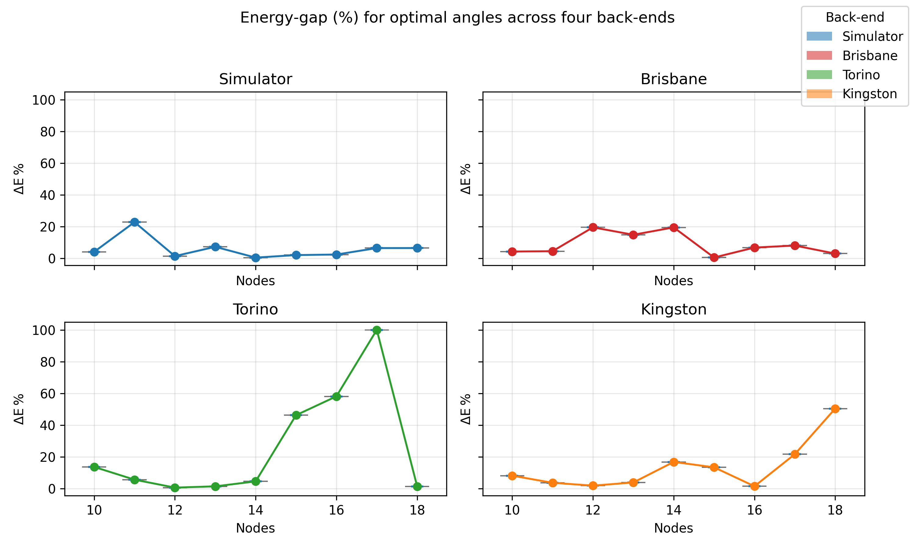
Figure 2: Energy gap $(\Delta E/E_{\text{ideal}})\times 100$ using the analytic angles on four IBM back-ends. The simulator stays within $\sim$5 %, while hardware gaps diverge once the compound error $C\!\gtrsim\!1$.

Using the parameter sets of Tables III, we executed each circuit $M=5\,000$ times on the ibm_brussels and ibm_kingston devices as well as the aer_simulator. For TSP we apply a lightweight feasibility repair to every measured bit-string—flipping the minimum number of bits to satisfy the “one city–one slot” constraints

On ibm_kingston the probe recovers optimal tours for wi4–wi5 and maintains $\Delta E/E_{\text{ideal}}\!<\!5\%$ up to 64 qubits with occasional errors that signify performance collapse, exactly as predicted by the run-to-failure metric. MaxCut problems shows a similar behaviour as documented in Figure 2.

Instance	$\mathcal{C}_{\text{opt}}$	$(\gamma,\beta)$	QAOA Dist.	Approx. Ratio	Gap (%)	Backend
wi4	6700	2.150,2.315	6700	1.000	0.00	aer_sim
			7149	0.937	6.70	ibm_brussels
			6700	1.000	0.00	ibm_kingston
wi5	6786	3.142,0.827	6888	0.984	1.51	aer_sim
			8898	0.762	31.1	ibm_brussels
wi6	9815	3.142,0.661	16023	0.612	63.3	ibm_brussels
			14502	0.677	47.8	ibm_kingston
wi7	7245	2.150,0.827	16753	0.433	131.2	ibm_brussels
dj8	2762	2.150,2.480	2822	0.979	2.17	ibm_kingston
dj9	2134	2.976,0.827	2567	0.832	20.3	ibm_kingston

TABLE IV: Hardware results for the TSP benchmark.

V Conclusion

We have presented a scalable, application-centred hardware-maturity probe built on single-layer QAOA with rigorously pre-computed parameters. Harmonic-analysis techniques yield closed-form bounds on the stationary points of the $p{=}1$ cost landscape, allowing the optimal angles $(\beta^{\star},\gamma^{\star})$ and reference energy $E_{\text{ideal}}$ to be obtained entirely offline. The benchmark therefore measures only what the quantum device must supply: faithful state preparation and read-out. Because the methodology uses analytic angles, touches the full quantum-classical stack, and applies unchanged to any device or workload, it constitutes a realistic, portable alternative to gate-level metrics and synthetic application suites. We envisage its adoption as a standard dependability yard-stick for emerging QHPC installations, guiding error-mitigation priorities today and tracking progress toward fault-tolerant advantage tomorrow.

References

- [1] J. Preskill, “Quantum Computing in the NISQ Era and Beyond,” Quantum, 2, 79 (2018).
- [2] E. Magesan, J. M. Gambetta, and J. Emerson, “Robust Randomized Benchmarking of Quantum Processes,” Phys. Rev. Lett., vol. 106, no. 18, p. 180504, 2011.
- [3] D. C. McKay, I. Hincks, E. J. Pritchett, M. Carroll, L. C. G. Govia, and S. T. Merkel, “Benchmarking Quantum Processor Performance at Scale,” arXiv preprint arXiv:2311.05933, 2023. [Online]. Available: https://arxiv.org/abs/2311.05933.
- [4] A. Wack, H. Paik, A. Javadi-Abhari, P. Jurcevic, I. Faro, J. M. Gambetta, and B. R. Johnson, “Quality, Speed, and Scale: three key attributes to measure the performance of near-term quantum computers,” arXiv preprint arXiv:2110.14108, 2021. [Online]. https://arxiv.org/abs/2110.14108.
- [5] E. Farhi, J. Goldstone, and S. Gutmann, “A Quantum Approximate Optimization Algorithm,” arXiv preprint arXiv:1411.4028, 2014.
- [6] E. Osaba and E. Villar-Rodriguez, “QOPTLib: A Quantum Computing Oriented Benchmark for Combinatorial Optimization Problems,” in Benchmarks and Hybrid Algorithms in Optimization and Applications, Springer Nature Singapore, 2023, pp. 49–63.
- [7] Ozaeta, A., van Dam, W., and McMahon, P. L., “Expectation values from the single-layer quantum approximate optimization algorithm on Ising problems,” Quantum Science and Technology 7, no. 4 (2022): 045036, http://dx.doi.org/10.1088/2058-9565/ac9013.
- [8] M. Benedetti, A. Perdomo-Ortiz, V. Leyton-Ortega, J. Realpe-Gómez, and J. I. Latorre, “Benchmarking near-term devices with quantum applications,” npj Quantum Information, vol. 6, pp. 1–8, 2020.
- [9] Wang, Z., Hadfield, S., Jiang, Z., and Rieffel, E. G., “Quantum approximate optimization algorithm for MaxCut: A fermionic view,” Phys Rev A 97, no. 2 (2018): 022304, http://dx.doi.org/10.1103/PhysRevA.97.022304.
- [10] O’Connor, P. and Kleyner, A., Practical Reliability Engineering, 5th ed., Wiley, 2012.
- [11] Modarres, M., Kaminskiy, M., and Krivtsov, V., Reliability Engineering and Risk Analysis: A Practical Guide, 3rd ed., CRC Press, 2009.
- [12] T. Tomesh, P. Gokhale, V. Omole, G. S. Ravi, K. N. Smith, J. Viszlai, X.-C. Wu, N. Hardavellas, M. R. Martonosi, and F. T. Chong, “SupermarQ: A Scalable Quantum Benchmark Suite,” arXiv:2202.11045 [quant-ph].
- [13] T. Lubinski, S. Johri, P. Varosy, J. Coleman, L. Zhao, J. Necaise, C. H. Baldwin, K. Mayer, and T. Proctor, “Application-Oriented Performance Benchmarks for Quantum Computing,” arXiv:2110.03137 [quant-ph] (2023), https://arxiv.org/abs/2110.03137.
- [14] M. Willsch, D. Willsch, F. Jin, H. De Raedt, and K. Michielsen, “Benchmarking the quantum approximate optimization algorithm,” Quantum Information Processing 19, no. 7 (2020). DOI: 10.1007/s11128-020-02692-8.
- [15] K. Michielsen, M. Nocon, D. Willsch, F. Jin, T. Lippert, and H. De Raedt, “Benchmarking gate-based quantum computers,” Computer Physics Communications 220, 44–55 (2017). DOI: 10.1016/j.cpc.2017.06.011.
- [16] J. A. Montañez-Barrera, K. Michielsen, and D. E. Bernal-Neira, “Evaluating the performance of quantum process units at large width and depth,” arXiv preprint, 2024.
- [17] A. Lucas, “Ising formulations of many NP problems,” Frontiers in Physics, vol. 2, 2014.
- [18] A. Zygmund, Trigonometric Series, 3rd ed. Cambr. Univ. Press, 2002.
- [19] S. C. Endres, C. Sandrock, and W. W. Focke, “A simplicial homology algorithm for Lipschitz optimisation,” Journal of Global Optimization, vol. 72, pp. 307–325, 2018.
- [20] C. Onah, “Single-Layer QAOA p = 1 Global-Optimum Catalogue (v1.0),” Zenodo, 2025, doi:10.5281/zenodo.15878141.