Solving the Trans-Planckian Censorship Problem with a Power-law Tail in $R^{2}$ Inflation: A Dynamical System Approach

Abstract

In this work we elaborate on solving the trans-Planckian censorship problem of standard slow-roll inflation by using a power-law inflationary tail generated by a scalar field with an exponential potential. We use a quantitative approach by studying in detail the phase space of a combined $F(R,\phi)$ cosmological system, focusing on the de Sitter and power-law subspaces of the total phase space. As we show, the de Sitter subspace of the $F(R,\phi)$ system shares the same fixed points as the vacuum $F(R)$ gravity system and the trajectories in the phase space tend to these fixed points. However, the power-law subspace is not stable and cannot be realized by the combined $F(R,\phi)$ system. To this end, we propose a well-motivated phenomenological $F(R)$ gravity model for which the $R^{2}$ term is switched off below a critical curvature near the end of the $R^{2}$ slow-roll inflationary era, and below that critical curvature, only the Einstein-Hilbert gravity term and the scalar field remain in the effective inflationary Lagrangian. The remaining system can successfully realize a power-law tail of the $R^{2}$ slow-roll era.

I Introduction

Understanding the primordial era of our Universe is one of the most prominent problems in modern theoretical physics. The most appealing and self-consistent description of the primordial era is inflation [1, 2, 3, 4] which remedies theoretically the shortcomings of the Standard Big Bang theory. The inflationary era belongs to the classical era of our Universe, means that the spacetime is four dimensional during inflation and the quantum modes that exit the Hubble horizon during the inflationary era, freeze and become classical after they exit the horizon. This is a standard requirement for inflationary theories, which shall concern us in this paper. Inflation can be realized in various contexts, for example in the context of General Relativity (GR) one can use a scalar field, minimally or non-minimally coupled with gravity [1, 2, 3, 4] but also modified gravity can realize the inflationary era, with the most prominent modified gravity theory [5, 6, 7, 8] being $F(R)$ gravity [9, 10, 11, 12, 13, 14, 15, 16, 17, 18, 19, 20, 21, 22], for various phenomenological and mathematical reasons. There are various motivations for using modified gravity to describe the Universe’s evolution, with the most strong motivation coming from the late-time cosmology. In the context of GR, the late-time evolution can be described by a cosmological constant, however the cosmological constant description of the dark energy era is not compatible with the latest DESI 2025 data [23] which point out that the dark energy is dynamical at an impressive 4.2$\sigma$ statistical confidence. Also even the Planck data indicate that the dark energy era might be described by a phantom equation of state (EoS) which in the context of GR can be realized by tachyon fields. Although tachyons are theoretically motivated by string theory, a consistent description of our Universe should avoid such scalar fields. Thus modified gravity seems to be a consistent proposal for the description of our Universe, and in fact it is possible that a unified description of inflation and the dark energy era can be provided by modified gravity and specifically $F(R)$ gravity, see for example the pioneer article [9] on this topic.

Inflation will be in the focus of many future experiments and collaborations, like the Simons observatory [24] and the future gravitational wave experiments [25, 26, 27, 28, 29, 30, 31, 32, 33]. The Simons observatory will probe directly the $B$-modes in the Cosmic Microwave Background (CMB) while the gravitational wave experiments will seek for a stochastic gravitational wave background generated by the inflationary era. In 2023 NANOGrav and other Pulsar Timing Arrays collaborations [34, 35, 36, 37] already reported the existence of a stochastic gravitational wave background, but it is highly unlikely that this background is due to inflation [38, 39].

Now, the question is which theory describes optimally the inflationary era. The answer is not easy, because there is motivation for having scalar fields and higher curvature terms in the inflationary effective Lagrangian. Hence, it might be possible that one cannot use one of the two descriptions, but one must include both scalars and higher order curvature invariants in the effective inflationary Lagrangian. The reason is simple and it is highly motivated by the quantum action of a scalar field. Specifically, the scalar field in its vacuum configuration can have at tree order the following action,

$$\mathcal{S}_{\varphi}=\int\mathrm{d}^{4}x\sqrt{-g}\left(\frac{1}{2}Z(\varphi)g^{\mu\nu}\partial_{\mu}\varphi\partial_{\nu}\varphi+\mathcal{V}(\varphi)+h(\varphi)R\right)\,,$$ (1)

and can be either conformally coupled or minimally coupled. The quantum corrected effective action of the scalar field in its vacuum configuration contains the following terms [40],

$$\mathcal{S}_{eff}=\int\mathrm{d}^{4}x\sqrt{-g}\Big(\Lambda_{1}+\Lambda_{2}R+\Lambda_{3}R^{2}+\Lambda_{4}R_{\mu\nu}R^{\mu\nu}+\Lambda_{5}R_{\mu\nu\alpha\beta}R^{\mu\nu\alpha\beta}+\Lambda_{6}\square R$$ (2)

$$+\Lambda_{7}R\square R+\Lambda_{8}R_{\mu\nu}\square R^{\mu\nu}+\Lambda_{9}R^{3}+\mathcal{O}(\partial^{8})+...\Big)\,,$$

and we included terms which make the action compatible with diffeomorphism invariance and also that terms contain up to fourth-order derivatives. Note that the parameters $\Lambda_{i}$, $i=1,2,...,6$ are dimensionful constants. Hence, a complete description of the effective inflationary Lagrangian might contain a scalar field along with higher order curvature invariants.

In a recent work, we used the combination of having a scalar field with exponential potential in the presence of an $R^{2}$ term in the inflationary Lagrangian as a possible solution of the trans-Planckian problem for the inflationary modes. We showed that if the slow-roll inflationary era, generated by an $R^{2}$ term, is followed by a power-law inflationary tail, generated by a scalar field with an exponential potential, the trans-Planckian issues of standard slow-roll inflation find a self-consistent remedy [41]. In the literature, having $R^{2}$ terms in the presence of a scalar field is quite common [42, 43, 44, 45, 46, 47, 48, 49, 50, 51], but in our approach, the scalar field has an exponential potential, which generates a power-law tail at the end of the inflationary era. However our previous study [41] was a qualitative approach based on the arguments that a power-law tail would actually remedy the Trans-Planckian Censorship Conjecture (TCC) [52, 53, 54, 55, 56, 57, 58, 59] issues of standard slow-roll inflation, if the scalar field dominates the evolution near the end of a standard $R^{2}$ slow-roll era. The question however is whether such a scenario can be realized by the cosmological system of an $R^{2}$-corrected exponential scalar theory. This question can be concretely answered if the phase space of the system is studied in detail. In this article, we perform a dynamical system analysis of the combined $R^{2}$ corrected scalar theory with the scalar having an exponential potential. We construct an autonomous dynamical system using appropriate dimensionless variables and we analyze in depth the phase space of the combined system, focusing on de Sitter and power-law subspaces of the total phase space. As we demonstrate, the de Sitter subspace is controlled by the $R^{2}$ gravity, since the trajectories in the phase space tend to the same fixed points that the vacuum $F(R)$ gravity has. This proves that indeed the $R^{2}$ gravity will realize a quasi-de Sitter era before the power-law inflationary era. However, the power-law subspace is quite unstable and it is highly unlikely that it can be physically realized by the combined $R^{2}$-scalar field system. Thus in order to solve the TCC issues of the standard slow-roll inflationary era generated by the $R^{2}$ gravity, one must use a phenomenological $F(R)$ gravity for which, below a critical curvature, the $R^{2}$ gravity is switched off and only Einstein-Hilbert gravity with a scalar field remains. This system can realize a pure power-law evolution, producing the desirable power-law tail that can solve the TCC problems of $R^{2}$ inflation. The phenomenological model of $F(R)$ gravity we will use is an exponential deformation of standard $R^{2}$ gravity, motivated by the positivity of the de Sitter perturbation scalaron mass [60].

This article is outlined as follows: In section II we review the mechanism of how a power-law tail in the standard quasi-de Sitter slow-roll $R^{2}$ era can solve the TCC problems of the vacuum $R^{2}$ gravity. In section III we study in depth the complete phase space of the $R^{2}$-corrected scalar field theory with exponential potential. By using appropriate dimensionless parameters we construct an autonomous dynamical system and we study its quasi-de Sitter and power-law phase spaces. As we show the de Sitter subspace is controlled by the $R^{2}$ gravity, however the power-law subspace is highly unstable and we show that it is highly unlikely that this can be physically realized. In section IV we propose a phenomenological $F(R)$ gravity model, which below a critical curvature near the end of the inflationary era, can switch off the $R^{2}$ term. We show that the remaining scalar system can generate the desired power-law tail of the $R^{2}$ era.

Before proceeding, in this work we shall use a flat Friedmann-Robertson-Walker (FRW) geometric background, with the line element being,

$$ds^{2}=-dt^{2}+a(t)^{2}\sum_{i=1,2,3}\left(dx^{i}\right)^{2}\,,$$ (3)

where $a(t)$ is as usual the scale factor and also the Ricci scalar for the FRW metric is,

$$R=6\left(\dot{H}+2H^{2}\right)\,,$$ (4)

where $H=\frac{\dot{a}}{a}$ stands for the Hubble rate.

II Overview of $f(R,\phi)$ Gravity Inflationary Framework and TCC Modes with Power-law Tail of $R^{2}$ Inflation

In this section we shall briefly provide a concrete overview of our previous work [41] and discuss the essential features of the idea that a power-law tail of a standard slow-roll $R^{2}$ inflationary theory can provide a remedy for the TCC problems of standard slow-roll inflation. We will base the presentation on our previous work Ref. [41] in order to provide the correct context for the next sections of this article. As we mentioned in the introduction, the standard slow-roll inflationary era, realized by minimally coupled scalar field theory or $R^{2}$ gravity, or any other modified gravity theory, has a serious issue related to the TCC [52, 53, 54, 55, 56, 57, 58, 59]. The TCC indicates that quantum inflationary modes with wavelengths that are trans-Planckian must not exit the Hubble horizon during the inflationary era and thus remain forever quantum and never enter the classical regime of modes outside the Hubble horizon. This TCC requirement for standard slow-roll inflationary regimes would impose severe conditions on the scale of inflation at the end of inflation which should be $V_{e}<10^{10}\,$GeV, which in turn imposes constraints on the tensor-to-scalar ratio to be $r<10^{-30}$. Apparently these two constraints eliminate most of the Planck-2018-compatible inflationary theories. In our previous work Ref. [41] however, we found a remedy for the TCC problems of standard slow-roll inflation. Recall that during the inflationary era, the Hubble horizon shrinks in a nearly inverse exponential way, due to the quasi-de Sitter evolution, and shrinks up to the point that the slow-roll condition breaks down, so when the first slow-roll index becomes of the order of unity. Now our approach in Ref. [41] was simple, we assumed that before the end of the $R^{2}$ slow-roll inflationary era, a scalar field with exponential potential dominates the evolution. Such a framework is known to produce a constant EoS evolution, as we now briefly show for completeness. Specifically, the scalar field is assumed to satisfy the following constraint,

$$\dot{\phi}^{2}=\beta V(\phi)\,,$$ (5)

hence,

$$\ddot{\phi}=\frac{\beta V^{\prime}}{2}\,.$$ (6)

The scalar field equation of motion is,

$$\ddot{\phi}+3H\dot{\phi}+V^{\prime}=0\,,$$ (7)

hence we have,

$$\left(\frac{\beta+2}{2}\right)^{2}\left(V^{\prime}\right)^{2}=9H^{2}\dot{\phi}^{2}\,,$$ (8)

or equivalently,

$$V=V_{0}e^{-\sqrt{\frac{6\beta}{\beta+2}}\kappa\phi}\,.$$ (9)

The exponential potential of Eq. (9) is exactly the form of the potential we shall use in this work. In the following we define the parameter $\lambda$ in the following way,

$$\lambda=\sqrt{\frac{6\beta}{\beta+2}}\,,$$ (10)

therefore the scalar field potential is written as,

$$V(\phi)=V_{0}\,e^{-\lambda\phi\kappa}\,.$$ (11)

Now such an evolution for the scalar field yields the following total EoS, if the evolution is scalar field dominated,

$$w_{\phi}=\frac{\beta-2}{\beta+2}\,.$$ (12)

The above evolution describes an inflationary power-law tail with a scale factor $a(t)=a_{0}\,t^{\eta}$, with $\eta=\frac{\beta+2}{3\beta}$, if $\beta<1$ and in the following we shall use the choice $\beta=0.99$ as we did in Ref. [41]. The way that the power-law inflationary tail of the $R^{2}$ era works is conceptually as follows: Following the arguments of Ref. [41, 57], the energy density of the scalar field after the end of the slow-roll inflationary era and when the power-law inflationary tail starts, is,

$$\rho_{\phi}\sim a^{-\frac{3\beta}{1+\frac{\beta}{2}}}\,.$$ (13)

The spatial flatness requirement is to [41, 57],

$$\left(\frac{a_{i}}{a_{R}}\right)^{2-\frac{3\beta}{1+\frac{\beta}{2}}}<10^{-2}\frac{T_{0}T_{eq}}{T_{R}^{2}}\,,$$ (14)

while in terms of the scalar field evolution and potential we have [41, 57],

$$\left(\frac{a_{i}}{a_{R}}\right)^{2-\frac{3\beta}{\sqrt{1+\frac{\beta}{2}}}}>\frac{T_{0}T_{eq}}{T_{R}^{2}}\,,$$ (15)

where $a_{i}$ is the value of the scale factor at the beginning of the inflationary power-law tail, $a_{R}$ is the scale factor at the end of the power-law inflationary tail, $T_{0}$ is the temperature of the Universe today, $T_{eq}$ is the temperature of the Universe at matter-radiation equality, and $T_{R}$ is the temperature of the Universe at the end of the power-law tail. Now when $\beta=0$ or equivalently $w_{\phi}\sim-1$, the inequality of Eq. (15) would be in conflict with that of Eq. (14). However, for larger values of $\beta$ in the range $0.5<\beta<1$ the two inequalities are intact. We will take $\beta\sim 0.99$ which yields a scalar field EoS parameter $w_{\phi}\sim-0.337793$. The TCC is solved as follows, the censorship itself is embodied in the following inequality,

$$\frac{a_{R}}{a_{i}}\ell_{pl}<H^{-1}(t_{R})\,,$$ (16)

where $\ell_{pl}$ is the Planck length. So following [41, 57] we get the resulting expression for the condition that is required to hold true if the TCC must be respected [41, 57],

$$\frac{T_{R}}{M_{p}}<\left(3/g^{*}\right)^{(1-\tilde{\beta})/(6-4\tilde{\beta})}\times 10^{-2/(6-4\tilde{\beta})}\left(\frac{T_{0}T_{eq}}{M_{p}}\right)^{1/(6-4\tilde{\beta})}\,,$$ (17)

where $\tilde{\beta}=\frac{3\beta}{\beta+2}$. Since in the case we are considering, we have $\beta=0.99$, we get, $T_{R}<10^{-30}\times M_{p}$, but this does not affect the flatness issue, which was solved due to the inequality (15) and due to the fact that an $R^{2}$ era precedes the power-law tail for a large number of $e$-foldings. Also such a low temperature at the end of the power-law tail does not affect the scalar perturbations or the tensor perturbations of the CMB because the power-law tail is detached from the $R^{2}$ slow-roll era. This is due to the fact that during the power-law tail the Hubble horizon shrinks in a much slower rate compared to the nearly inverse de Sitter Hubble horizon shrinking. Thus, the power-law tail also contributes to the CMB, but possibly these modes have wavelengths much shorted than 10Mpc, hence although these modes exit from the Hubble horizon during the power-law inflationary tail, do not affect the CMB at least linearly. At these wavelengths the CMB is non-linear.

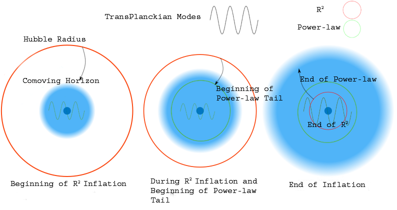
Figure 1: Schematic presentation of the resolution of TCC problems offered by the power-law inflationary tail following a standard $R^{2}$ slow-roll inflationary era. When the $R^{2}$ slow-roll inflationary era commences (red circle, left figure) the Hubble horizon is large and all the inflationary modes are contained in it. As the slow-roll inflationary era proceeds, the inflationary modes gradually exit the Hubble horizon and become classical (right figure, red circle). If no power-law era follows right after the $R^{2}$ slow-roll era, the Trans-Planckian modes would also exit the horizon (red circle, right figure), hence we invoked an inflationary power-law tail that follows the standard $R^{2}$ slow-roll era (green circle, figure at the center). During the power-law inflationary tail, the Hubble horizon shrinks more slowly compared to the de Sitter shrinking of the $R^{2}$ era, therefore the Trans-Planckian modes never exit the Hubble horizon and never become classical (green circle, right figure). Hence, this slowing down of the shrinking rate of the Hubble horizon during the power-law inflationary tail is what solves the TCC problems of standard slow-roll inflation.

Let us illustrate schematically our way of thinking on how a power-law inflationary tail might solve the TCC problems of standard $R^{2}$ slow-roll inflation. In Fig. 2 we present the various steps of the resolution we proposed in Ref. [41] in a schematic way. Let us describe the procedure that is depicted in Fig. 2. At the beginning of the $R^{2}$ slow-roll inflationary era the Hubble horizon (red circle, left figure) is large and all the inflationary modes are contained in it. As the slow-roll inflationary era proceeds, more and more modes exit the Hubble horizon and become classical (right figure, red circle). If no power-law era follows the $R^{2}$ slow-roll era, the trans-Planckian modes would also exit the horizon (red circle, right figure), so we invoked an inflationary power-law tail to follow the $R^{2}$ era (green circle, figure at the center). Now during the power-law inflationary tail, the Hubble horizon shrinks more slowly compared to the de Sitter shrinking of the $R^{2}$ era, thus the trans-Planckian modes never exit the Hubble horizon (green circle, right figure) and thus never become classical. Hence, this slowing down of the shrinking rate of the Hubble horizon during the power-law inflationary tail, is what solves the TCC problems of slow-roll inflation. Of course, it is notable that several inflationary modes of the power-law tail inflationary era will contribute to the CMB. However, since the shrinking rate of the power-law tail is small, it is possible that the modes that exit the horizon have a wavelength smaller than $10$Mpc, thus these modes contribute to the non-linear parts of the CMB.

Now the important question we asked in our previous work [41] but we did not address formally, is whether our scenario is realized by the combined field equations of the $R^{2}$-scalar field system, since we required a clean power-law inflationary tail in which the $R^{2}$ gravity will not dominate the evolution. This study is the core part of this work and is presented in the next sections.

III Study of the Complete $F(R,\phi)$ Gravity Phase Space for de Sitter and Power-law Cases

In this section we will study the complete phase space of the $F(R,\phi)$ gravity system. We will focus on the case that the parameter $\beta$ in the scalar field subsystem is $\beta=0.99$ and we examine the phase space using an autonomous dynamical system that we will extract using the field equations. Our aim is to see whether the total phase space of the system contains the power-law tail controlled by the scalar field at the end of the $R^{2}$ inflation. Also we shall answer the question whether the $R^{2}$ term drives the quasi-de Sitter evolution of the combined scalar-$F(R)$ gravity system. Our results are striking since it proves that the power-law cosmology is never realized by the $F(R,\phi)$ gravity system, but we also prove that the $R^{2}$ term indeed realizes a quasi-de Sitter era for the combined scalar-$F(R)$ gravity system. In fact, as we will show the only inflationary evolution that can be realized by the $F(R,\phi)$ gravity system is the de Sitter evolution. Let us get into the details of our analysis to present concretely these striking results.

We start with the combined $F(R,\varphi)$ gravitational action which has the form,

$$\centering\mathcal{S}=\int{d^{4}x\sqrt{-g}\left(\frac{F(R)}{2\kappa^{2}}-\frac{1}{2}g^{\mu\nu}\partial_{\mu}\varphi\partial_{\nu}\varphi-\mathcal{V}(\varphi)\right)}\,,\@add@centering$$ (18)

with $\kappa^{2}=8\pi G=\frac{1}{Mp^{2}}$ and also $M_{p}$ stands for the reduced Planck mass. Varying the gravitational action with respect to the metric tensor and with respect to the scalar field, we obtain the following field equations,

$$3H^{2}F_{R}=\frac{RF_{R}-F}{2}-3H\dot{F}_{R}+\kappa^{2}\left(\frac{1}{2}\dot{\phi}^{2}+V(\phi)\right)\,,$$ (19)

$$-2\dot{H}F=\kappa^{2}\dot{\phi}^{2}+\ddot{F}_{R}-H\dot{F}_{R}+\frac{4\kappa^{2}}{3}\rho_{r}\,,$$

$$\ddot{\phi}+3H\dot{\phi}+V^{\prime}(\phi)=\frac{Q}{\dot{\phi}}\,,$$ (20)

where $F_{R}=\frac{\partial F}{\partial R}$ and we shall use these in order to construct an autonomous dynamical system which controls the dynamics of the $F(R,\phi)$ gravity system. The autonomous dynamical system of $F(R)-\phi$ gravity system can easily be obtained if we make use of the following dimensionless parameters,

$$x_{1}=-\frac{\dot{F}_{R}(R)}{F_{R}(R)H},\,\,\,x_{2}=-\frac{F(R)}{6F_{R}(R)H^{2}},\,\,\,x_{3}=\frac{R}{6H^{2}},\,\,\,x_{4}=\frac{\kappa}{H}\sqrt{\frac{V}{3}},\,\,\,x_{5}=\frac{\kappa\dot{\phi}}{H},\,\,\,x_{6}=\frac{1}{F_{R}}\,,$$ (21)

Recall that the scalar field potential is assumed to be equal to $V(\phi)=V_{0}\,e^{-\lambda\phi}$ with $\lambda$ defined in Eq. (10), see also Eq. (9). We shall express the dynamical variable of the system to be the $e$-foldings number instead of the cosmic time. So by using the dimensionless variables (21) and the field equations (19) and (20), we obtain the following autonomous dynamical system,

$$\frac{\mathrm{d}x_{1}}{\mathrm{d}N}=x_{1}^{2}-x_{1}x_{3}+3x_{1}+2x_{3}+x_{5}^{2}x_{6}-4\,,$$ (22)

$$\frac{\mathrm{d}x_{2}}{\mathrm{d}N}=m+x_{1}x_{2}-2x_{2}x_{3}+4x_{2}-4x_{3}+8\,,$$

$$\frac{\mathrm{d}x_{3}}{\mathrm{d}N}=-m-2x_{3}^{2}+8x_{3}-8\,,$$

$$\frac{\mathrm{d}x_{4}}{\mathrm{d}N}=-x_{3}x_{4}-\frac{\lambda x_{4}x_{5}}{2}+2x_{4}\,,$$

$$\frac{\mathrm{d}x_{5}}{\mathrm{d}N}=-x_{5}+3\lambda x_{4}^{2}-x_{5}x_{3}\,,$$

$$\frac{\mathrm{d}x_{6}}{\mathrm{d}N}=x_{1}x_{6}\,.$$

with the parameter $m$ being defined to be,

$$m=-\frac{\ddot{H}}{H^{3}}\,.$$ (23)

Now, the dynamical system of Eq. (22) is not entirely autonomous unless the parameter $m$ is a constant. This is true for the cases of interest, that is for a quasi-de Sitter evolution of the form $H(t)=H_{0}-H_{I}\,t$ and for a power-law evolution of the form $H(t)=\frac{\eta}{t}$, with $\eta=\frac{\beta+2}{3\beta}$, which describes the power-law tail inflationary tail that is controlled by the scalar field, if $\beta<1$. For the quasi-de Sitter evolution, we have that $m=0$ and for the power-law inflationary tail we have $m=-\frac{2}{\eta^{2}}$, so in both cases the dynamical system is autonomous. The effective EoS, defined as,

$$w_{eff}=-1-\frac{2\dot{H}}{3H^{2}}\,,$$ (24)

can be written in terms of the parameters of the dynamical system, and specifically it reads,

$$w_{eff}=-\frac{1}{3}(2x_{3}-1)\,.$$ (25)

Our aim in this section is to investigate in depth the phase space of the $F(R,\phi)$ system, revealing any periodicity features and stable attractors, for the power-law case, in which $m=-\frac{2}{\eta^{2}}$ with $\eta=\frac{\beta+2}{3\beta}$ and for the $m=0$ case. Let us start with the power-law inflationary tail case, which interests us the most. Our aim is to reveal whether the dynamical system reaches the attractor for which the total EoS is $w_{eff}=\frac{\beta-2}{\beta+2}$. If the system reaches a stable attractor, which yields $w_{eff}=\frac{\beta-2}{\beta+2}$ then this would be a proof that the power-law tail indeed dominates the evolution compared to the $R^{2}$ gravity. Unfortunately our results indicate that this is not true. For $\beta=0.99$ we found unstable and saddle fixed points for the system, and also none of the fixed points is reached by the phase space trajectories, which strongly diverge after a few $e$-foldings. Let us start the analysis by presenting the fixed points of the system (22) for $\beta=0.99$, which are listed in Table 1.

Table 1: The Fixed Points of the Dynamical System of Eq. (22) for $\beta=0.99$ and $m=-\frac{2}{\eta^{2}}$ with $\eta=\frac{\beta+2}{3\beta}$.

Name of Fixed Point	Fixed Point Values for $\beta=0.99$
$P_{1}^{*}$	$(x^{*}_{1},x^{*}_{2},x^{*}_{3},x^{*}_{4}x^{*}_{5},x^{*}_{6})=(-2.72291,2.71622,1.00669,0,0,0)$	Saddle
$P_{2}^{*}$	$(x^{*}_{1},x^{*}_{2},x^{*}_{3},x^{*}_{4}x^{*}_{5},x^{*}_{6})=(0.729596,-0.736285,1.00669,0,0,0)$	Saddle
$P_{3}^{*}$	$(x^{*}_{1},x^{*}_{2},x^{*}_{3},x^{*}_{4}x^{*}_{5},x^{*}_{6})=(-2.72291,2.71622,1.00669,-0.817861,1.40948,0)$	Saddle
$P_{4}^{*}$	$(x^{*}_{1},x^{*}_{2},x^{*}_{3},x^{*}_{4}x^{*}_{5},x^{*}_{6})=(-2.72291,2.71622,1.00669,0.817861,1.40948,0)$	Saddle
$P_{5}^{*}$	$(x^{*}_{1},x^{*}_{2},x^{*}_{3},x^{*}_{4}x^{*}_{5},x^{*}_{6})=(0,-1.00669,1.00669,-0.817861,1.40948,1)$	Saddle
$P_{6}^{*}$	$(x^{*}_{1},x^{*}_{2},x^{*}_{3},x^{*}_{4}x^{*}_{5},x^{*}_{6})=(0,-1.00669,1.00669,0.817861,1.40948,1)$	Saddle
$P_{7}^{*}$	$(x^{*}_{1},x^{*}_{2},x^{*}_{3},x^{*}_{4}x^{*}_{5},x^{*}_{6})=(0.729596,-0.736285,1.00669,-0.817861,1.40948,0)$	Saddle
$P_{8}^{*}$	$(x^{*}_{1},x^{*}_{2},x^{*}_{3},x^{*}_{4}x^{*}_{5},x^{*}_{6})=(0.729596,-0.736285,1.00669,0.817861,1.40948,0)$	Saddle

All the fixed points of the dynamical system of Eq. (22) are unstable and share a common property, $w_{eff}=-0.337793=\frac{\beta-2}{\beta+2}$. So basically the total EoS is described by a scalar field dominated evolution, hence the power-law inflationary tail is realized indeed. However, the dynamics in the phase space indicate that these unstable fixed points are never reached, regardless the initial conditions we choose. It seems that, although the fixed points are indeed unstable, the phase space trajectories never reach the unstable fixed points and blow-up in the trajectory space as a function of the $e$-foldings. To show this, in Fig. 2 we present the trajectories in the phase space of the dynamical system (22) for the initial conditions $x_{1}(0)=-0.01$, $x_{2}(0)=0.01$, $x_{3}(0)=2.05$, $x_{4}(0)=0$, $x_{5}(0)=7$, $x_{6}(0)=-2$, and for $m=-\frac{2}{\eta^{2}}$, $\beta=0.99$.

Figure 2: Numerical solutions of the trajectories $x_{1}(N)$, $x_{2}(N)$, $x_{3}(N)$, $x_{4}(N)$, $x_{5}(N)$ and $x_{6}(N)$ for the dynamical system (22), using the initial conditions $x_{1}(0)=-0.01$, $x_{2}(0)=0.01$, $x_{3}(0)=2.05$, $x_{4}(0)=0$, $x_{5}(0)=7$, $x_{6}(0)=-2$, and for $m=-\frac{2}{\eta^{2}}$, $\beta=0.99$.

As it can be seen in Fig. 2 the trajectories blow-up in the phase space and the fixed points are never reached. Now this said behavior occurs for quite a large number of initial condition sets. Thus the dynamical system is extremely unstable and one cannot claim easily that the scalar field dominates the evolution. This would happen for example if initial conditions existed for which the dynamical system would be attracted on the fixed points and then would be repelled from these. This does not happen, so the only scenario for which the TCC issues can be resolved using a power-law evolution is the one which eliminates the $F(R)$ gravity once a specific curvature scale is reached before the end of the $R^{2}$ inflation. In this way, the $F(R)$ gravity would reduce to a simple Einstein-Hilbert gravity and the dynamical system (22) would no longer be valid. Such a scenario will be presented in the next section.

Now it is worth discussing the de Sitter subspace of the total phase space of the dynamical system (22). Recall that in this case, $m=0$, thus let us analyze the de Sitter scenario in order to reveal how the phase space behaves in this case. We start with the fixed points of the system, with $\beta=0.99$ and these are presented in Table 2.

Table 2: The Fixed Points of the Dynamical System of Eq. (22) for $\beta=0.99$ and $m=0$.

Name of Fixed Point	Fixed Point Values for $\beta=0.99$	Stability
$P_{1}^{*}$	$(x^{*}_{1},x^{*}_{2},x^{*}_{3},x^{*}_{4}x^{*}_{5},x^{*}_{6})=(0,x_{2},2,0,0,x_{6})$	Unstable
$P_{2}^{*}$	$(x^{*}_{1},x^{*}_{2},x^{*}_{3},x^{*}_{4}x^{*}_{5},x^{*}_{6})=(0,x_{2},2,0,0,0)$	Unstable
$P_{3}^{*}$	$(x^{*}_{1},x^{*}_{2},x^{*}_{3},x^{*}_{4}x^{*}_{5},x^{*}_{6})=(-1,0,2,0,0,0)$	Unstable

As it can be seen in Table 2, the dynamical system of Eq. (22) for the de-Sitter subspace has three unstable fixed points. The phase space structure is quite interesting in this case, since it has some lower dimensional stability as we show shortly, but also has an inherent consistency, compared with the previous power-law case, because the trajectories in the phase space tend to the fixed point $P_{3}^{*}$. We can clearly show this by solving numerically the dynamical system (22) using various initial conditions. Our results are presented in Fig. 3, using the initial conditions $x_{1}(0)=-5$, $x_{2}(0)=-5$, $x_{3}(0)=2.5$, $x_{4}(0)=-5$, $x_{5}(0)=-0.2$, $x_{6}(0)=1$, and for $m=0$ and $\beta=0.99$.

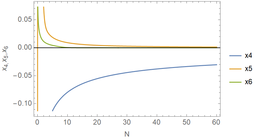
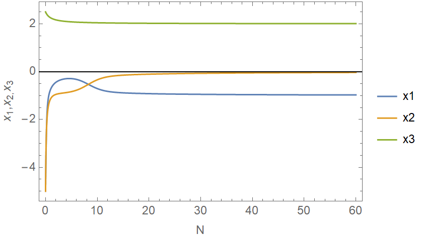
Figure 3: Numerical solutions of the dynamical system (22) $x_{1}(N)$, $x_{2}(N)$, $x_{3}(N)$, $x_{4}(N)$, $x_{5}(N)$ and $x_{6}(N)$ using the initial conditions $x_{1}(0)=-5$, $x_{2}(0)=-5$, $x_{3}(0)=2.5$, $x_{4}(0)=-5$, $x_{5}(0)=-0.2$, $x_{6}(0)=1$, and for $m=0$ and $\beta=0.99$.

As we can see in Fig. 3 all the solutions tend to the fixed point $P_{3}^{*}$, however the parameter $x_{6}$ does not reach the fixed point value $x_{6}=0$ even after 60 $e$-foldings. This feature is true for a large number of sets of initial conditions. The behavior of the trajectories though shows some formal stable fixed point dynamical evolution, because eventually the fixed point $P_{3}^{*}$ is reached by most of the variables. Also the total EoS is $w_{eff}=-1$ due to the fact that $x_{3}=2$, recall Eq. (25) which relates the total EoS with the parameter $x_{3}$. It is worth studying more the de Sitter subspace of the total phase space, so let us consider some structures that can be found in the phase space for $m=0$. Let us start with the Principal Component Analysis (PCA) which can reveal the actual dynamics of the dynamical system of Eq. (22) and reduce the dimensionality of the dynamical system, using only the fast variables that determine truly the dynamics of the system. If the dynamical system of Eq. (22) has intrinsic lower-dimensional structure, the PCA projection can in principle reveal it. If the first three components in the PCA projection have or generate some characteristic structure or pattern, then the six-dimensional initial system of Eq. (22) effectively behaves like a three- dimensional one. If the projection does not preserve any key features whatsoever, more dimensions may be needed for the analysis. We shall use the PCA analysis in order to reveal the dominant modes of the dynamical system of Eq. (22) and the results of our PCA analysis can be found in Fig. 4. Apparently, the resulting pattern indicates the presence of multiple isolated stable fixed points, with no signs of periodicity or chaos. This is somewhat exciting due to the presence of the unstable fixed points we presented earlier for the dynamical system of Eq. (22). The lower-dimensional subspace of the total phase space seems stable though, thus there must be an inherent structure in the dynamical system.

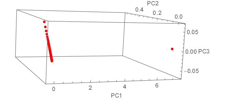
Figure 4: PCA analysis of the dynamical system of Eq. (22).

Now it is worth examining the Poincare sections of the dynamical system of Eq. (22). The Poincare sections reduce the complexity of the dynamical system and indicate which variables drive the dynamical evolution. In Figs. 5 and we present the Poincare sections corresponding to $x_{6}=0$. As it can be seen, there exist various isolated points of equilibrium that capture the dynamics and it seems that the variable $x_{6}$ does not affect significantly the dynamics of the system. Both the Poincare sections and the PCA analysis indicate the existence of isolated stable points for various initial conditions, however no periodicity or chaos is revealed in the dynamical system of Eq. (22).

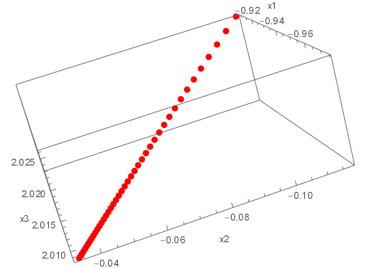
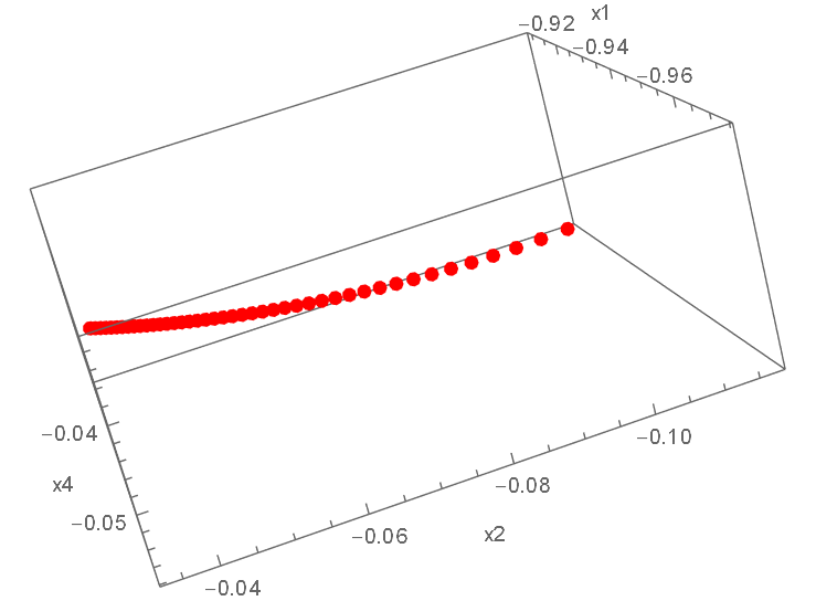
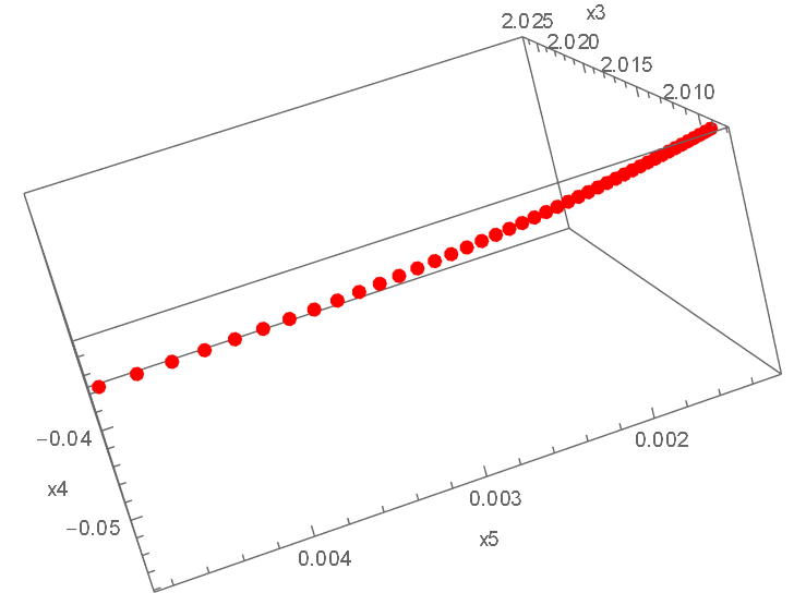
Figure 5: Poincare section $x_{6}=0$ and dynamics for various variables of the dynamical system of Eq. (22.

Now the intriguing question is whether $F(R)$ gravity dominates the evolution over the scalar field with exponential potential. Let us get into some details on this and we start with the EoS of the scalar field which is defined as,

$$w_{\phi}=\frac{\frac{\dot{\phi}^{2}}{2}-V}{\frac{\dot{\phi}^{2}}{2}+V}\,,$$ (26)

and for the potential chosen as in Eq. (9) it should result to Eq. (12) and for $\beta=0.99$ should take the value $w_{\phi}=-0.337793$. We can express the scalar field EoS (26) in terms of the variables $x_{4}$ and $x_{5}$ defined in Eq. (21) and we have,

$$w_{\phi}=\frac{\frac{x_{5}^{2}}{2}-3x_{4}^{2}}{\frac{x_{5}^{2}}{2}+3x_{4}^{2}}\,.$$ (27)

We can plot the scalar field EoS of Eq. (27) as a function of the $e$-foldings and this done in Fig. 5.

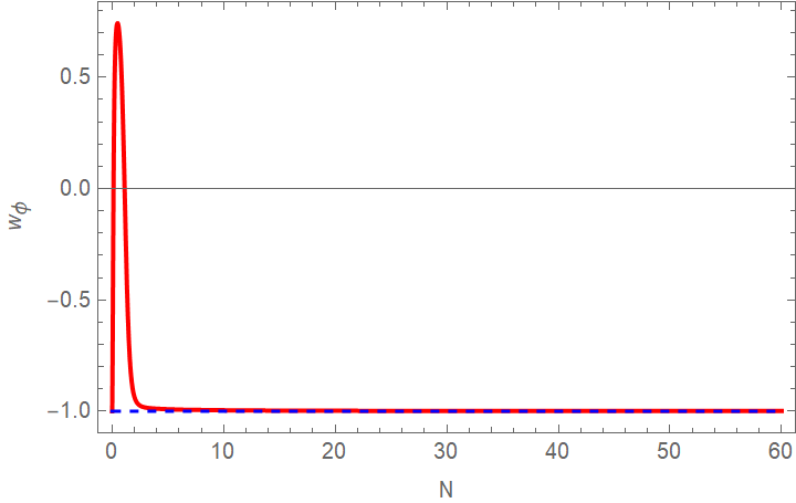
Figure 6: The scalar field EoS $w_{\phi}$ as a function of the $e$-foldings number, for the dynamical system (22) with initial conditions $x_{1}(0)=-5$, $x_{2}(0)=-5$, $x_{3}(0)=2.5$, $x_{4}(0)=-5$, $x_{5}(0)=-0.2$, $x_{6}(0)=1$, and for $m=0$ and $\beta=0.99$.

As it can be seen in Fig. 6 the behavior of the scalar field EoS is intriguing because after a few $e$-foldings it settles in the value $w_{\phi}\simeq-1$, which contradicts the expected value $w_{\phi}=-0.337793$ that it should have. Now it is worth recalling the pure $F(R)$ gravity phase space in order to completely understand what is going on in this obscure situation. The analysis of the pure $F(R)$ gravity phase space was performed in Ref. [61] so at this point we shall recall the essential features and results of that analysis. When the $F(R)$ gravity phase space is considered solely, the following variables are used,

$$x_{1}=-\frac{\dot{F_{R}}(R)}{F_{R}(R)H},\,\,\,x_{2}=-\frac{F(R)}{6F_{R}(R)H^{2}},\,\,\,x_{3}=\frac{R}{6H^{2}}\,,$$ (28)

and the pure $F(R)$ gravity dynamical system becomes,

$$\frac{\mathrm{d}x_{1}}{\mathrm{d}N}=-4-3x_{1}+2x_{3}-x_{1}x_{3}+x_{1}^{2}\,,$$ (29)

$$\frac{\mathrm{d}x_{2}}{\mathrm{d}N}=8+m-4x_{3}+x_{2}x_{1}-2x_{2}x_{3}+4x_{2}\,,$$

$$\frac{\mathrm{d}x_{3}}{\mathrm{d}N}=-8-m+8x_{3}-2x_{3}^{2}\,,$$

where $m$ is again,

$$m=-\frac{\ddot{H}}{H^{3}}\,.$$ (30)

The dynamical system of Eq. (29) has the following fixed points,

$$\phi_{*}^{1}=(-1,0,2),\,\,\,\phi_{*}^{2}=(0,-1,2)\,,$$ (31)

with $\phi_{*}^{1}$ being the stable fixed point and the other fixed point $\phi_{*}^{2}$ is the unstable one with both the fixed points being de Sitter fixed points, since , since for both $x_{3}=2$ and hence, the total EoS is $w_{eff}=-1$. Now let us compare the trajectories of the pure $F(R)$ gravity and the $F(R,\phi)$ gravity phase space. This is done in Fig. 7, where we plot the trajectories for the variables $x_{1}$, $x_{2}$ and $x_{3}$ for the pure $F(R)$ gravity dynamical system (29) and for the $F(R,\phi)$ dynamical system (22) with initial conditions $x_{1}(0)=-5$, $x_{2}(0)=-5$, $x_{3}(0)=2.5$, $x_{4}(0)=-5$, $x_{5}(0)=-0.2$, $x_{6}(0)=1$, and for $m=0$ and $\beta=0.99$. With red curves we plot the trajectories of the pure $F(R)$ gravity dynamical system (29) and with blue curves the $F(R,\phi)$ dynamical system (22). As it can be seen in Fig. 7, the two systems share the same fixed points, since the variables $x_{1}$, $x_{2}$ and $x_{3}$ have the same behavior after some $e$-foldings. However, we need to note that the fixed point is unstable in the combined $F(R,\phi)$ dynamical system (22) while it is stable in the pure $F(R)$ gravity dynamical system (29).

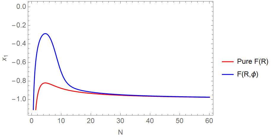
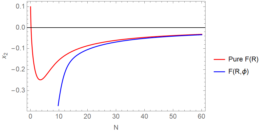
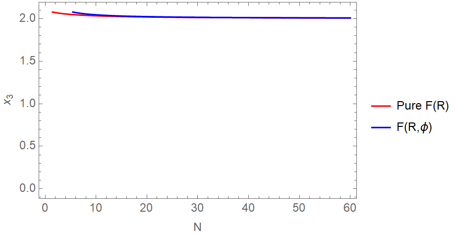
Figure 7: Plot of the trajectories for the variables $x_{1}$, $x_{2}$ and $x_{3}$ for the pure $F(R)$ gravity dynamical system (29) and for the combined $F(R,\phi)$ dynamical system (22) with the initial conditions being chosen as $x_{1}(0)=-5$, $x_{2}(0)=-5$, $x_{3}(0)=2.5$, $x_{4}(0)=-5$, $x_{5}(0)=-0.2$, $x_{6}(0)=1$. We used $m=0$ and $\beta=0.99$ for the case of the $F(R,\phi)$ dynamical system (22). The red curves correspond to the trajectories of the pure $F(R)$ gravity dynamical system (29) and the blue curves correspond to the $F(R,\phi)$ dynamical system (22). The two systems share the same fixed points, because the variables $x_{1}$, $x_{2}$ and $x_{3}$ converge to the same fixed point in the phase space.

By looking Fig. 7 one thing is certain, it seems that the $F(R)$ gravity controls the dynamics if the evolution is a de Sitter one, and as we saw earlier, for the power-law tail evolution, the dynamical system is strongly unstable with the trajectories blowing up and never reaching the existing unstable fixed points. Thus, in order for the power-law inflationary tail to solve the TCC problems of standard inflation, one needs to eliminate effectively the non-trivial $F(R)$ part from the field equations, thus leaving a pure scalar field dominated evolution. We present an effective theory of this sort in the next section.

IV A Way to Satisfy the TCC Requirements: Choice of a Suitable $F(R)$ Gravity that Ensures an Exact Scalar Field Driven Power-law Inflationary Tail

As we demonstrated in the previous sections, in order for the power-law tail to control the dynamics of inflation for the last $e$-foldings of the inflationary era, one must clearly cut off the non-linear $F(R)$ gravity part. In this section we shall use a phenomenological $F(R)$ gravity model which can actually allow the power-law tail to be realized. The model we shall use is a exponential deformation of the $R^{2}$ model, of the form,

$$F(R)=R+\frac{R^{2}}{2M^{2}}+\tanh\left(\frac{R-R_{c}}{\Lambda}\right)\,\frac{R^{2}}{2M^{2}}+f_{DE}(\frac{R}{\Lambda})\,.$$ (32)

These models are highly motivated by arguments related to the unified description of inflation with the dark energy era, as was demonstrated in Ref. [60]. The term $f_{DE}(\frac{R}{\Lambda})$ can be chosen on the phenomenological basis of Ref. [60] and can be a power-law term of the Ricci scalar, or some exponential model. This term however cannot dominate over the scalar field at late times, due to the fact that the scalar field potential parameter $V_{0}$ in Eq. (9) is constrained by the Planck data [62] to be $V_{0}\simeq 9\times 10^{-11}M_{p}^{4}$ thus the scalar potential would certainly dominate over a wide range of dark energy driving $F(R)$ gravity terms. So let us focus on the inflationary era, in which case the $f_{DE}(\frac{R}{\Lambda})$ part is strongly subdominant and both the scalar field and $R^{2}$ terms dominate over it. Now let us demonstrate how the $F(R)$ gravity behaves during the inflationary era. The critical scalar curvature $R_{c}$ in Eq. (32) corresponds to the value of the curvature scalar when the power-law tail should take over the control of the dynamics of the cosmological evolution, so it corresponds to some curvature near the end of the slow-roll era. The behavior of the term $\tanh\left(\frac{R-R_{c}}{\Lambda}\right)$ during the inflationary era is,

$$\tanh\left(\frac{R-R_{c}}{\Lambda}\right)=\left\{\begin{array}[]{c}1,\,\,\,\mathrm{when}\,\,\,R>R_{c}\\ 0,\,\,\,\mathrm{when}\,\,\,R\sim R_{c}\\ -1,\,\,\,\mathrm{when}\,\,\,R<R_{c}\,,\end{array}\right.$$ (33)

Thus the $F(R)$ gravity function of Eq. (32) behaves in the following way during the inflationary era,

$$F(R)=\left\{\begin{array}[]{c}R+\frac{R^{2}}{M^{2}},\,\,\,\mathrm{when}\,\,\,R>R_{c}\\ R+\frac{R^{2}}{2M^{2}},\,\,\,\mathrm{when}\,\,\,R\sim R_{c}\\ R,\,\,\,\mathrm{when}\,\,\,R<R_{c}\,,\end{array}\right.$$ (34)

Hence, with the phenomenological choice of Eq. (32) the $R^{2}$ part of the $F(R)$ gravity is effectively switched off during the last stages of inflation. At the beginning of the inflationary era, the $F(R)$ gravity controls the dynamics with the dominant $R^{2}$ term driving the evolution, then once the curvature lowers down to the critical value $R_{c}$ the $F(R)$ gravity is basically described by an Einstein-Hilbert term. We have shown this in Fig. 8 where we present the behavior of the $F(R)$ gravity during the inflationary era, taking $R_{c}\sim 10^{10}\,$eV² as an example, and using the phenomenological values of $M$ and $\Lambda$. As it can be seen in Fig. 8, when the curvature lowers below the critical curvature, $R_{c}\sim 10^{10}\,$eV², the $R^{2}$ term is switched off and the effective $F(R)$ gravity is described by the Einstein-Hilbert term solely.

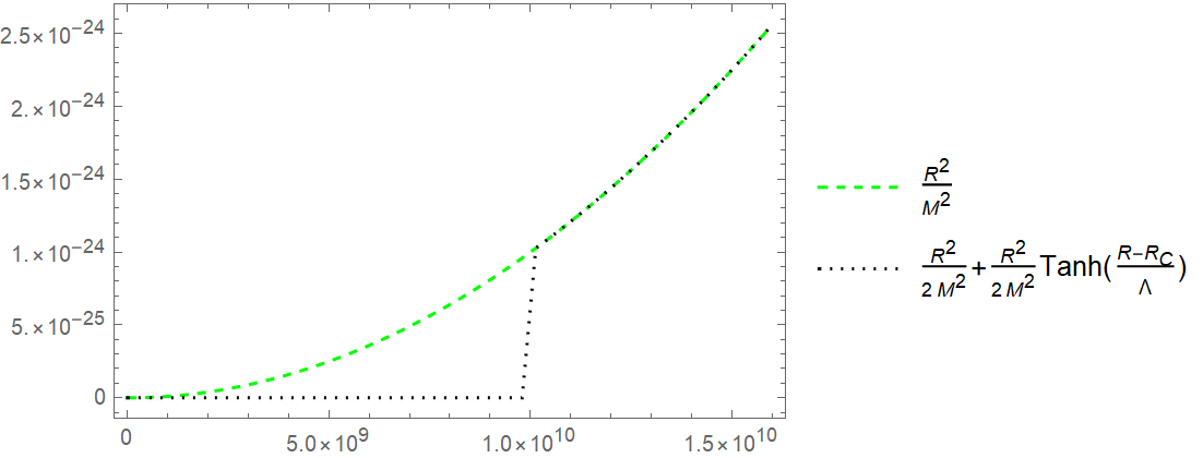
Figure 8: The comparison of the $\frac{R^{2}}{2M^{2}}+\tanh\left(\frac{R-R_{c}}{\Lambda}\right)\,\frac{R^{2}}{2M^{2}}$ and $\frac{R^{2}}{M^{2}}$ terms for $R_{c}\sim 10^{10}\,$eV². As it can be seen, when the curvature lowers below the critical value $R_{c}$, the $\frac{R^{2}}{2M^{2}}+\tanh\left(\frac{R-R_{c}}{\Lambda}\right)\,\frac{R^{2}}{2M^{2}}$ term is effectively zero.

Thus with the choice of Eq. (32), the scalar field basically dominates the evolution for values of the curvature lower the critical curvature $R_{c}$, and therefore, the Friedmann equation becomes,

$$3H^{2}=\frac{\kappa^{2}\dot{\phi}^{2}}{2}+V\,.$$ (35)

Also the total EoS parameter $w_{tot}$ for the scalar field dominated inflationary epoch is,

$$w_{tot}=\frac{P_{\phi}}{\rho_{\phi}}=w_{\phi}\Omega_{\phi}\,,$$ (36)

Using the dimensionless variables,

$$x^{2}=\frac{\kappa^{2}\dot{\phi}^{2}}{6H^{2}},\,\,\,y^{2}=\frac{\kappa^{2}V}{3H^{2}}\,,$$ (37)

we have for the scalar EoS parameter and the energy density,

$$w_{\phi}=\frac{x^{2}-y^{2}}{x^{2}+y^{2}},\,\,\,\Omega_{\phi}=x^{2}+y^{2}=1\,,$$ (38)

and we can construct the following autonomous dynamical system for the scalar field [63],

$$\frac{\mathrm{d}x}{\mathrm{d}N}=-3x+\frac{\lambda\sqrt{6}}{2}y^{2}+\frac{3x}{2}\left(1+x^{2}-y^{2}\right)\,,$$ (39)

$$\frac{\mathrm{d}y}{\mathrm{d}N}=-\frac{\lambda\sqrt{6}}{2}x\,y+\frac{3y}{2}\left(1+x^{2}-y^{2}\right)\,,$$

using again the $e$-foldings number $N$ as the dynamical variable. For $\beta=0.99$ the fixed points of the system, their stability, and their physical significance are presented in Table 3. As it can be seen, the only physically acceptable fixed points are $P_{1}^{*}$, $P_{3}^{*}$ and $P_{4}^{*}$ and from these the only stable are $P_{3}^{*}$ and $P_{4}^{*}$ which perfectly describe the desired EoS parameter value $w_{tot}=-0.337793$ which corresponds to the scalar field for $\beta=0.99$.

Table 3: Phase Space Fixed Points, Stability and Physical Significance of the Dynamical System (39) for $\beta=0.99$.

Name of Fixed Point	Fixed Point Values for $\beta=0.99$	Stability	$\Omega_{\phi}$	$w_{\phi}$
$P_{1}^{*}$	$(x_{*},y_{*})=(-1,0)$	unstable	1	1
$P_{2}^{*}$	$(x_{*},y_{*})=(0,0)$	unstable
$P_{3}^{*}$	$(x_{*},y_{*})=(0.575416,-0.817861)$	stable	1	-0.337793
$P_{4}^{*}$	$(x_{*},y_{*})=(0.575416,0.817861)$	stable	1	-0.337793
$P_{5}^{*}$	$(x_{*},y_{*})=(0.868936,0.868936)$	unstable	1.5101	0
$P_{6}^{*}$	$(x_{*},y_{*})=(0.868936,-0.868936)$	unstable	1.5101	0

Also, in Fig. 9 we present the phase space trajectories of the dynamical system (39), including with red dots the fixed points $P_{3}^{*}=(x_{*},y_{*})=(0.575416,-0.817861)$ and $P_{4}^{*}=(x_{*},y_{*})=(0.575416,0.817861)$ as red dots. As it can be seen in Fig. 9, all the trajectories in the phase space of the dynamical system (39) are attracted to the stable fixed points $P_{3}^{*}$ and $P_{4}^{*}$. Thus, in this section we showed that if the non-linear part of the $F(R)$ gravity is switched off near the end of the slow-roll era, the dynamics of the cosmological system is clearly dominated by the scalar field, driving the system to the fixed points $P_{3}^{*}=(x_{*},y_{*})=(0.575416,-0.817861)$ and $P_{4}^{*}=(x_{*},y_{*})=(0.575416,0.817861)$ which yield an EoS parameter $w_{tot}=-0.337793$.

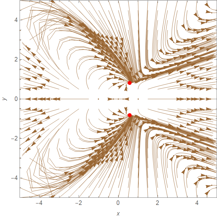
Figure 9: Phase space trajectories for the dynamical system (39) for various initial conditions. The red dots represent the fixed points $P_{3}^{*}=(x_{*},y_{*})=(0.575416,-0.817861)$ and $P_{4}^{*}=(x_{*},y_{*})=(0.575416,0.817861)$.

Now as a final comment it would be interesting to consider the late-time dynamics of the resulting quintessence-like theory which is controlled by the scalar field. The scalar field potential would dominate over a wide range of dark energy $F(R)$ gravity models as we mentioned at the beginning of this section, if the scalar field values are close to the Planck scale $M_{p}$. This study however exceeds the purposes of this work and we leave it for future work.

V The Graceful Exit from Inflation Issue with Power-law Inflation

The power-law inflationary regime yields a constant first slow-roll index, thus it is not possible to end inflation in this scenario, if the scalar field $\phi$ that drives the power-law era is considered by itself without the presence of other fields. However, the scalar field $\phi$ is a remnant of some ultraviolet completion of the standard model, thus it may have couplings to other scalar fields and also to fermions. These couplings may actually end the inflationary regime controlled by the scalar field. In this section we shall present two mechanisms that may end the inflationary era controlled by the scalar field, the first mechanism employs an auxiliary scalar field $\chi$, a so-called waterfall field, thus giving rise to some sort of hybrid inflation [69, 70, 71, 72, 73], and the second employs the coupling of the scalar field $\phi$ to a fermion [74, 75]. Let us analyze in detail these two mechanisms.

Before starting, it is important to discuss why ending the power-law inflationary era is important. Specifically, why the graceful exit from inflation is important, and how this will help resolving completely the Trans-Planckian issues of inflation. The exit from inflation is important. So after the power-law inflationary era is realized, the Hubble horizon still shrinks, but in a slower way compared with the slow-roll era. Hence the Hubble horizon shrinks slowly, thus if inflation lasted for ever, the Trans-Planckian modes would exit the horizon eventually. Thus inflation must end, this is why we proposed two mechanisms that may end the power-law inflation era, and thus provide a complete resolution for the Trans-Planckian issue.

V.1 Hybrid Inflation with a Waterfall Field

For the Hybrid inflation we shall consider the scalar field $\phi$ and its coupling to a waterfall-type auxiliary scalar field $\chi$. The scalar field $\phi$ will play the role of the inflaton and slowly rolls in a power-law way and drives inflation, while the waterfall field $\chi$ will end the inflationary regime of the field $\phi$ through a symmetry-breaking instability caused by the effective potential of the two scalars. The proposed potential could have the following form, the potential is given by:

$$V(\phi,\chi)=V_{0}e^{-\lambda\phi/M_{p}}+\frac{1}{2}g^{2}\phi^{2}\chi^{2}+\frac{\lambda_{\chi}}{4}\left(\chi^{2}-v^{2}\right)^{2},$$ (40)

where $g$ is the coupling constant between the scalar field $\phi$ and the waterfall field $\chi$. The interaction coupling $\lambda_{\chi}$ and also $v$ define the symmetry-breaking sector of the waterfall field $\chi$. During the power-law inflation, the field $\chi$ is stabilized at $\chi=0$ due to its large positive effective mass for sufficiently large $\phi$. Hence, the inflationary trajectory follows the line $\chi=0$ and the effective mass of the waterfall field is,

$$m_{\chi}^{2}(\phi)=\frac{\partial^{2}V(\phi,\chi)}{\partial\chi^{2}}\Big|_{\chi=0}=-\lambda_{\chi}v^{2}+g^{2}\phi^{2}\,,$$ (41)

and the critical inflaton value $\phi_{c}$ at which the effective mass of the waterfall field is zero is equal to,

$$m_{\chi}^{2}(\phi_{c})=0\quad\Rightarrow\quad\phi_{c}=\frac{\sqrt{\lambda_{\chi}}}{g}v.$$ (42)

Then we have the following symmetry breaking pattern in the $\chi$-sector: For $\phi>\phi_{c}$, we have $m_{\chi}^{2}>0$ and $\chi=0$, thus the waterfall scalar is stable around the origin in the $\chi$ direction of the effective potential. For $\phi<\phi_{c}$, we have $m_{\chi}^{2}<0$ and therefore the $\chi=0$ minimum becomes unstable, thus this instability triggers a rapid symmetry-breaking transition. Hence in this mechanism, inflation ends when the scalar field $\phi$ reaches the critical value $\phi_{c}$ at which point, the effective mass squared of the waterfall field $\chi$ becomes negative. The field $\chi$ rapidly rolls to its true vacuum situated at the value $\chi=\pm v$, thus ending the inflationary regime of the scalar field $\phi$ via a second-order (or sometimes first-order) phase transition, hence the name waterfall scalar field [69, 73]. In the context of this mechanism one can even have a grasp on the total duration of the power-law regime, because inflation ends on the critical value of the scalar field $\phi_{c}$ which depends on the symmetry breaking in the $\chi$ sector. Note that in this case, the free couplings of the inflation $\phi$ to the waterfall scalar does not affect the power-law inflationary phase, it affects only though the ending of the power-law phase which can be controlled by $\phi_{c}=\frac{\sqrt{\lambda_{\chi}}}{g}v$. Thus the model is open for rich phenomenology in the post-power-law inflationary phase.

V.2 Ending Power-law Inflation with Fermion Loops

Another way to terminate the power-law inflation regime of the scalar field $\phi$ is to add interactions of the scalar field with fermions, and consider quantum corrections arising from the fermionic interactions which can modify the inflaton potential and thus provide a graceful exit to the power-law regime [74, 75]. Let us introduce a Yukawa interaction between the scalar field $\phi$ and a Dirac fermion $\psi$, of the form

$$\mathcal{L}_{\text{int}}=-y\phi\bar{\psi}\psi,$$ (43)

where $y$ is the Yukawa coupling. This Yukawa interaction gives the following effective mass to the Dirac fermion $m_{\psi}(\phi)=y\phi$. At the quantum level, the Yukawa interaction modifies the scalar field potential through one-loop radiative corrections, and specifically, through the Coleman-Weinberg one-loop effective potential. This Dirac fermion one-loop correction to the scalar field effective potential has the following form [74, 75],

$$\Delta V_{\text{1-loop}}(\phi)=-\frac{N_{f}}{8\pi^{2}}m_{\psi}^{4}(\phi)\ln\left(\frac{m_{\psi}^{2}(\phi)}{\mu^{2}}\right),$$ (44)

where $N_{f}$ is the number of fermionic degrees of freedom and $\mu$ is the renormalization scale. Substituting $m_{\psi}(\phi)=y\phi$, the total scalar field effective potential becomes

$$V_{\text{eff}}(\phi)=V_{0}e^{-\lambda\phi/M_{p}}-\frac{N_{f}y^{4}\phi^{4}}{8\pi^{2}}\ln\left(\frac{y^{2}\phi^{2}}{\mu^{2}}\right)\,,$$ (45)

therefore, the first slow-roll index is no longer constant, and thus inflation can come to an end. Both the fermion loop and the waterfall mechanism have their inherent appeal, however the waterfall mechanism offers more possibilities for model building. Also it is possible to end inflation by using particle creation, although this type of scenarios is used in warm inflation frameworks. Finally, we need to note that in the fermion loop case, the Yukawa coupling might affect the duration of the inflationary phase, in order to have a significant duration for the power-law case, one must choose the Yukawa coupling accordingly. For example we plotted the effective potential $V_{eff}(\phi)$ versus the ordinary potential $V(\phi)$ for various values of the Yukawa coupling $y$ in Fig. 10 and it can clearly be seen how the Yukawa coupling affects the form of the potential.

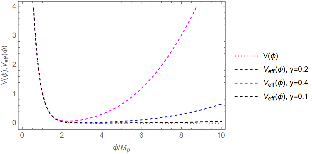
Figure 10: The effective potential $V_{eff}(\phi)$ versus the ordinary potential $V(\phi)$ for various values of the Yukawa coupling $y$. We used $y=0.1$ (black curve), $y=0.4$ (blue curve) and $y=0.9$ (magenta curve), while we chose the renormalization scale to be $\mu=10\,M_{p}$.

As it can be seen in Fig. 10, the exponential potential is similar for all the cases for small values of the scalar field, sub-Planck ones specifically, but the potential deviates significantly for large values of the Yukawa coupling for trans-Planckian values of the scalar field, when the Yukawa coupling is larger than $y\sim 0.1$. Hence, one must choose small values of the Yukawa coupling, if this mechanism is to function properly, without significantly affecting the power-law inflationary regime. However, the presence of the logarithm always affects the final form of the potential and even terminates the power-law era, which is the important feature of these radiative fermion loops. Specifically, the most optimal scenario for our analysis, based on Fig. 10 would be the case with $y=0.1$ or even smaller Yukawa coupling. The scenario does not deviate from the power-law evolution, and also it is also possible to terminate the power-law inflationary era. To see this, let us recall that the first slow-roll index has the form, $\epsilon=\frac{M_{p}^{2}}{2}\left(\frac{V^{\prime}(\phi)}{V(\phi)}\right)^{2}$, so for the effective potential (45) the first slow-roll index takes the form,

$$\epsilon=\frac{2M_{p}^{2}\left(4\pi^{2}\lambda V_{0}+2y^{4}\phi^{3}e^{\lambda\phi}\log\left(\frac{y^{2}\phi^{2}}{\mu^{2}}\right)+y^{4}\phi^{3}e^{\lambda\phi}\right)^{2}}{\left(y^{4}\phi^{4}e^{\lambda\phi}\log\left(\frac{y^{2}\phi^{2}}{\mu^{2}}\right)-8\pi^{2}V_{0}\right)^{2}}\,,$$ (46)

so solving the equation $\epsilon(\phi)=1$ might be impossible in order to see whether inflation terminates. We can do a numerical plot to reveal this, so in Fig. 11 we plot the behavior of the first slow-roll index (46) as a function of the scalar field for $\mu=10\,M_{p}$ and $y=0.1$.

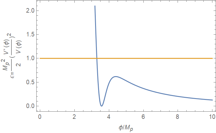
Figure 11: The first slow-roll index, $\epsilon=\frac{M_{p}^{2}}{2}\left(\frac{V^{\prime}(\phi)}{V(\phi)}\right)^{2}$ for the effective potential $V_{eff}(\phi)$ for $y=0.1$ and $\mu=10\,M_{p}$. As it can be seen, the first slow-roll index crosses the $\epsilon=1$ line and thus the power-law inflationary era is possible to end.

As it can be seen in Fig. 11, the first slow-roll index $\epsilon$ has the desirable behavior since it is smaller than unity for larger values of the scalar field, and as the scalar field values drop, it becomes unity (it crosses the $\epsilon=1$ orange line) for some model-dependent value of the scalar field, which for the case at hand is $\phi\sim 3.5\,M_{p}$. Hence, it is possible for this fermion-loop mechanism to end the power-law inflationary era, without affecting significantly the power-law behavior of the potential. One can also choose much smaller Yukawa couplings to achieve a better behavior of the potential too, and also appropriately choose the renormalization scale. However this analysis exceeds by far the aims of this work, so we refrain from going into details.

VI Conclusions and Discussion

In this work we analyzed quantitatively a scenario which can solve the TCC problems of standard slow-roll inflation. Specifically we considered an $R^{2}$-corrected scalar field theory with an exponential scalar potential. This theoretical framework can remedy the TCC problems of slow-roll inflation, if the $R^{2}$ gravity drives the slow-roll era and, near its end, it is followed by a power-law inflationary era generated by the scalar field with exponential potential. This scenario was developed in Ref. [41] using a qualitative approach which focused on the phenomenology and in this work we aimed to quantitatively study the $R^{2}$-corrected scalar field theory with an exponential scalar potential using a detailed phase space analysis. We constructed an autonomous dynamical system for the $F(R,\phi)$ system using appropriate dimensionless variables and the field equations and we studied two solution subspaces of the total phase space, the de Sitter subspace and the power-law evolution subspace. The study of the de Sitter subspace validated our approach that the $F(R)$ gravity would indeed dominate the evolution if it is described by a quasi-de Sitter Hubble rate. Specifically, we showed that the trajectories in the phase space are attracted to the same fixed points that vacuum $F(R)$ gravity has. On the contrary, the power-law evolution cannot be realized by the $F(R,\phi)$ system because the phase space is highly unstable. To this end, we indicated that in order to solve the TCC problems of standard slow-roll inflation, one needs an exact power-law tail following the standard $R^{2}$-driven slow-roll era, which can be solely realized by a scalar field. Thus, when the curvature reaches a critical value near the end of the slow-roll era, the $R^{2}$ gravity term in the $F(R,\phi)$ system must be switched off. We presented a well-motivated phenomenological $F(R)$ gravity model of this sort and we demonstrated that for curvatures below a critical curvature near the end of the slow-roll era, the cosmological system is composed by an Einstein-Hilbert term and a scalar field with exponential potential, which can realize the desired power-law tail of the $R^{2}$ gravity slow-roll era, and thus solve the TCC problems of the latter.

We also briefly discussed some implications of this work, having to do with the existence of a quintessential scalar field theory in the post inflationary era. This scalar field is also present at late times and thus could be responsible for the dark energy era, but we did not analyze this scenario in detail because it is out of the context of the present work. Another interesting feature of the scenario discussed in this work is related to the total EoS of the system in the post-inflationary era and specifically during the reheating, which can in principle have even observational implications, for example in gravitational waves, see for example [64]. Also in this work we essentially considered a quantum corrected scalar field action with the scalar field being in its vacuum configuration, hence one can in principle consider more general quantum corrections [65, 66, 67] and the phenomenology of such models could give us interesting insights on the primordial Universe. Finally, let us note that this realization of a slow-roll era ending up to a power-law evolution could also be realized by a constant-roll to slow-roll transition as was performed in Ref. [68]. We aim to discuss whether such a transition can resolve the TCC issues of standard slow-roll inflation in a future work. This extension may incorporate methods and fixed points that emerged from Refs. [76, 77], which contain extensions of the modified gravity sector, which we did not considered in this work.

References

- [1] A. D. Linde, Lect. Notes Phys. 738 (2008) 1 [arXiv:0705.0164 [hep-th]].
- [2] D. S. Gorbunov and V. A. Rubakov, “Introduction to the theory of the early universe: Cosmological perturbations and inflationary theory,” Hackensack, USA: World Scientific (2011) 489 p;
- [3] A. Linde, arXiv:1402.0526 [hep-th];
- [4] S. D. Odintsov, V. K. Oikonomou, I. Giannakoudi, F. P. Fronimos and E. C. Lymperiadou, Symmetry 15 (2023) no.9, 1701 doi:10.3390/sym15091701 [arXiv:2307.16308 [gr-qc]].
- [5] S. Nojiri, S. D. Odintsov and V. K. Oikonomou, Phys. Rept. 692 (2017) 1 [arXiv:1705.11098 [gr-qc]].
-
[6]
S. Capozziello, M. De Laurentis,
Phys. Rept. 509, 167 (2011);
V. Faraoni and S. Capozziello, Fundam. Theor. Phys. 170 (2010). - [7] S. Nojiri, S.D. Odintsov, eConf C0602061, 06 (2006) [Int. J. Geom. Meth. Mod. Phys. 4, 115 (2007)].
- [8] S. Nojiri, S.D. Odintsov, Phys. Rept. 505, 59 (2011);
- [9] S. Nojiri and S. D. Odintsov, Phys. Rev. D 68 (2003), 123512 doi:10.1103/PhysRevD.68.123512 [arXiv:hep-th/0307288 [hep-th]].
- [10] S. Capozziello, V. F. Cardone and A. Troisi, Phys. Rev. D 71 (2005), 043503 doi:10.1103/PhysRevD.71.043503 [arXiv:astro-ph/0501426 [astro-ph]].
- [11] J. c. Hwang and H. Noh, Phys. Lett. B 506 (2001), 13-19 doi:10.1016/S0370-2693(01)00404-X [arXiv:astro-ph/0102423 [astro-ph]].
- [12] G. Cognola, E. Elizalde, S. Nojiri, S. D. Odintsov and S. Zerbini, JCAP 02 (2005), 010 doi:10.1088/1475-7516/2005/02/010 [arXiv:hep-th/0501096 [hep-th]].
- [13] Y. S. Song, W. Hu and I. Sawicki, Phys. Rev. D 75 (2007), 044004 doi:10.1103/PhysRevD.75.044004 [arXiv:astro-ph/0610532 [astro-ph]].
- [14] T. Faulkner, M. Tegmark, E. F. Bunn and Y. Mao, Phys. Rev. D 76 (2007), 063505 doi:10.1103/PhysRevD.76.063505 [arXiv:astro-ph/0612569 [astro-ph]].
- [15] G. J. Olmo, Phys. Rev. D 75 (2007), 023511 doi:10.1103/PhysRevD.75.023511 [arXiv:gr-qc/0612047 [gr-qc]].
- [16] I. Sawicki and W. Hu, Phys. Rev. D 75 (2007), 127502 doi:10.1103/PhysRevD.75.127502 [arXiv:astro-ph/0702278 [astro-ph]].
- [17] V. Faraoni, Phys. Rev. D 75 (2007), 067302 doi:10.1103/PhysRevD.75.067302 [arXiv:gr-qc/0703044 [gr-qc]].
- [18] S. Carloni, P. K. S. Dunsby and A. Troisi, Phys. Rev. D 77 (2008), 024024 doi:10.1103/PhysRevD.77.024024 [arXiv:0707.0106 [gr-qc]].
- [19] S. Nojiri and S. D. Odintsov, Phys. Lett. B 657 (2007), 238-245 doi:10.1016/j.physletb.2007.10.027 [arXiv:0707.1941 [hep-th]].
- [20] N. Deruelle, M. Sasaki and Y. Sendouda, Prog. Theor. Phys. 119 (2008), 237-251 doi:10.1143/PTP.119.237 [arXiv:0711.1150 [gr-qc]].
- [21] S. A. Appleby and R. A. Battye, JCAP 05 (2008), 019 doi:10.1088/1475-7516/2008/05/019 [arXiv:0803.1081 [astro-ph]].
- [22] P. K. S. Dunsby, E. Elizalde, R. Goswami, S. Odintsov and D. S. Gomez, Phys. Rev. D 82 (2010), 023519 doi:10.1103/PhysRevD.82.023519 [arXiv:1005.2205 [gr-qc]].
- [23] M. Abdul Karim et al. [DESI], [arXiv:2503.14738 [astro-ph.CO]].
- [24] M. H. Abitbol et al. [Simons Observatory], Bull. Am. Astron. Soc. 51 (2019), 147 [arXiv:1907.08284 [astro-ph.IM]].
- [25] S. Hild, M. Abernathy, F. Acernese, P. Amaro-Seoane, N. Andersson, K. Arun, F. Barone, B. Barr, M. Barsuglia and M. Beker, et al. Class. Quant. Grav. 28 (2011), 094013 doi:10.1088/0264-9381/28/9/094013 [arXiv:1012.0908 [gr-qc]].
- [26] J. Baker, J. Bellovary, P. L. Bender, E. Berti, R. Caldwell, J. Camp, J. W. Conklin, N. Cornish, C. Cutler and R. DeRosa, et al. [arXiv:1907.06482 [astro-ph.IM]].
- [27] T. L. Smith and R. Caldwell, Phys. Rev. D 100 (2019) no.10, 104055 doi:10.1103/PhysRevD.100.104055 [arXiv:1908.00546 [astro-ph.CO]].
- [28] J. Crowder and N. J. Cornish, Phys. Rev. D 72 (2005), 083005 doi:10.1103/PhysRevD.72.083005 [arXiv:gr-qc/0506015 [gr-qc]].
- [29] T. L. Smith and R. Caldwell, Phys. Rev. D 95 (2017) no.4, 044036 doi:10.1103/PhysRevD.95.044036 [arXiv:1609.05901 [gr-qc]].
- [30] N. Seto, S. Kawamura and T. Nakamura, Phys. Rev. Lett. 87 (2001), 221103 doi:10.1103/PhysRevLett.87.221103 [arXiv:astro-ph/0108011 [astro-ph]].
- [31] S. Kawamura, M. Ando, N. Seto, S. Sato, M. Musha, I. Kawano, J. Yokoyama, T. Tanaka, K. Ioka and T. Akutsu, et al. [arXiv:2006.13545 [gr-qc]].
- [32] A. Weltman, P. Bull, S. Camera, K. Kelley, H. Padmanabhan, J. Pritchard, A. Raccanelli, S. Riemer-Sørensen, L. Shao and S. Andrianomena, et al. Publ. Astron. Soc. Austral. 37 (2020), e002 doi:10.1017/pasa.2019.42 [arXiv:1810.02680 [astro-ph.CO]].
- [33] P. Auclair et al. [LISA Cosmology Working Group], [arXiv:2204.05434 [astro-ph.CO]].
- [34] G. Agazie et al. [NANOGrav], doi:10.3847/2041-8213/acdac6 [arXiv:2306.16213 [astro-ph.HE]].
- [35] J. Antoniadis, P. Arumugam, S. Arumugam, S. Babak, M. Bagchi, A. S. B. Nielsen, C. G. Bassa, A. Bathula, A. Berthereau and M. Bonetti, et al. [arXiv:2306.16214 [astro-ph.HE]].
- [36] D. J. Reardon, A. Zic, R. M. Shannon, G. B. Hobbs, M. Bailes, V. Di Marco, A. Kapur, A. F. Rogers, E. Thrane and J. Askew, et al. doi:10.3847/2041-8213/acdd02 [arXiv:2306.16215 [astro-ph.HE]].
- [37] H. Xu, S. Chen, Y. Guo, J. Jiang, B. Wang, J. Xu, Z. Xue, R. N. Caballero, J. Yuan and Y. Xu, et al. doi:10.1088/1674-4527/acdfa5 [arXiv:2306.16216 [astro-ph.HE]].
- [38] S. Vagnozzi, JHEAp 39 (2023), 81-98 doi:10.1016/j.jheap.2023.07.001 [arXiv:2306.16912 [astro-ph.CO]].
- [39] V. K. Oikonomou, Phys. Rev. D 108 (2023) no.4, 043516 doi:10.1103/PhysRevD.108.043516 [arXiv:2306.17351 [astro-ph.CO]].
- [40] A. Codello and R. K. Jain, Class. Quant. Grav. 33 (2016) no.22, 225006 doi:10.1088/0264-9381/33/22/225006 [arXiv:1507.06308 [gr-qc]].
- [41] S. D. Odintsov and V. K. Oikonomou, [arXiv:2504.04561 [gr-qc]].
- [42] Y. Ema, Phys. Lett. B 770 (2017), 403-411 doi:10.1016/j.physletb.2017.04.060 [arXiv:1701.07665 [hep-ph]].
- [43] Y. Ema, K. Mukaida and J. Van De Vis, JHEP 02 (2021), 109 doi:10.1007/JHEP02(2021)109 [arXiv:2008.01096 [hep-ph]].
- [44] V. R. Ivanov and S. Y. Vernov, [arXiv:2108.10276 [gr-qc]].
- [45] S. Gottlober, J. P. Mucket and A. A. Starobinsky, Astrophys. J. 434 (1994), 417-423 doi:10.1086/174743 [arXiv:astro-ph/9309049 [astro-ph]].
- [46] V. M. Enckell, K. Enqvist, S. Rasanen and L. P. Wahlman, JCAP 01 (2020), 041 doi:10.1088/1475-7516/2020/01/041 [arXiv:1812.08754 [astro-ph.CO]].
- [47] J. Kubo, J. Kuntz, M. Lindner, J. Rezacek, P. Saake and A. Trautner, JHEP 08 (2021), 016 doi:10.1007/JHEP08(2021)016 [arXiv:2012.09706 [hep-ph]].
- [48] D. Gorbunov and A. Tokareva, Phys. Lett. B 788 (2019), 37-41 doi:10.1016/j.physletb.2018.11.015 [arXiv:1807.02392 [hep-ph]].
- [49] X. Calmet and I. Kuntz, Eur. Phys. J. C 76 (2016) no.5, 289 doi:10.1140/epjc/s10052-016-4136-3 [arXiv:1605.02236 [hep-th]].
- [50] V. K. Oikonomou, Annals Phys. 432 (2021), 168576 doi:10.1016/j.aop.2021.168576 [arXiv:2108.04050 [gr-qc]].
- [51] V. K. Oikonomou and I. Giannakoudi, Nucl. Phys. B 978 (2022), 115779 doi:10.1016/j.nuclphysb.2022.115779 [arXiv:2204.02454 [gr-qc]].
- [52] J. Martin and R. H. Brandenberger, Phys. Rev. D 63 (2001), 123501 doi:10.1103/PhysRevD.63.123501 [arXiv:hep-th/0005209 [hep-th]].
- [53] R. H. Brandenberger and J. Martin, Mod. Phys. Lett. A 16 (2001), 999-1006 doi:10.1142/S0217732301004170 [arXiv:astro-ph/0005432 [astro-ph]].
- [54] A. Bedroya and C. Vafa, JHEP 09 (2020), 123 doi:10.1007/JHEP09(2020)123 [arXiv:1909.11063 [hep-th]].
- [55] R. Brandenberger, LHEP 2021 (2021), 198 doi:10.31526/lhep.2021.198 [arXiv:2102.09641 [hep-th]].
- [56] R. Brandenberger and V. Kamali, Eur. Phys. J. C 82 (2022) no.9, 818 doi:10.1140/epjc/s10052-022-10783-2 [arXiv:2203.11548 [hep-th]].
- [57] V. Kamali and R. Brandenberger, Phys. Rev. D 101 (2020) no.10, 103512 doi:10.1103/PhysRevD.101.103512 [arXiv:2002.09771 [hep-th]].
- [58] A. Berera, Phys. Rev. Lett. 75 (1995), 3218-3221 doi:10.1103/PhysRevLett.75.3218 [arXiv:astro-ph/9509049 [astro-ph]].
- [59] R. Brandenberger, [arXiv:2503.17659 [astro-ph.CO]].
- [60] V.K. Oikonomou, [arXiv:2504.00915 [gr-qc]].
- [61] S. D. Odintsov and V. K. Oikonomou, Phys. Rev. D 96 (2017) no.10, 104049 doi:10.1103/PhysRevD.96.104049 [arXiv:1711.02230 [gr-qc]].
- [62] Y. Akrami et al. [Planck], Astron. Astrophys. 641 (2020), A10 doi:10.1051/0004-6361/201833887 [arXiv:1807.06211 [astro-ph.CO]].
- [63] C. G. Boehmer, G. Caldera-Cabral, R. Lazkoz and R. Maartens, Phys. Rev. D 78 (2008), 023505 doi:10.1103/PhysRevD.78.023505 [arXiv:0801.1565 [gr-qc]].
- [64] S. Pi, M. Sasaki, A. Wang and J. Wang, Phys. Rev. D 110 (2024) no.10, 103529 doi:10.1103/PhysRevD.110.103529 [arXiv:2407.06066 [astro-ph.CO]].
- [65] S. P. Miao, N. C. Tsamis and R. P. Woodard, [arXiv:2409.12003 [gr-qc]].
- [66] S. P. Miao, N. C. Tsamis and R. P. Woodard, [arXiv:2405.01024 [gr-qc]].
- [67] S. P. Miao, N. C. Tsamis and R. P. Woodard, JHEP 07 (2024), 099 doi:10.1007/JHEP07(2024)099 [arXiv:2405.00116 [gr-qc]].
- [68] S. D. Odintsov and V. K. Oikonomou, JCAP 04 (2017), 041 doi:10.1088/1475-7516/2017/04/041 [arXiv:1703.02853 [gr-qc]].
- [69] G. N. Felder, L. Kofman and A. D. Linde, Phys. Rev. D 64 (2001), 123517 doi:10.1103/PhysRevD.64.123517 [arXiv:hep-th/0106179 [hep-th]].
- [70] A. D. Linde, Phys. Rev. D 49 (1994), 748-754 doi:10.1103/PhysRevD.49.748 [arXiv:astro-ph/9307002 [astro-ph]].
- [71] E. J. Copeland, A. R. Liddle, D. H. Lyth, E. D. Stewart and D. Wands, Phys. Rev. D 49 (1994), 6410-6433 doi:10.1103/PhysRevD.49.6410 [arXiv:astro-ph/9401011 [astro-ph]].
- [72] E. J. Copeland, A. R. Liddle and J. E. Lidsey, Phys. Rev. D 64 (2001), 023509 doi:10.1103/PhysRevD.64.023509 [arXiv:astro-ph/0006421 [astro-ph]].
- [73] H. M. Lee and A. G. Menkara, Phys. Rev. D 107 (2023) no.11, 115019 doi:10.1103/PhysRevD.107.115019 [arXiv:2304.08686 [hep-ph]].
- [74] S. R. Coleman and E. J. Weinberg, Phys. Rev. D 7 (1973), 1888-1910 doi:10.1103/PhysRevD.7.1888
- [75] N. Bostan and V. N. Şenoğuz, JCAP 10 (2019), 028 doi:10.1088/1475-7516/2019/10/028 [arXiv:1907.06215 [astro-ph.CO]].
- [76] S. Capozziello, F. Occhionero and L. Amendola, Int. J. Mod. Phys. D 1 (1993), 615-639 doi:10.1142/S0218271892000318
- [77] S. Carloni, P. K. S. Dunsby, S. Capozziello and A. Troisi, Class. Quant. Grav. 22 (2005), 4839-4868 doi:10.1088/0264-9381/22/22/011 [arXiv:gr-qc/0410046 [gr-qc]].