SymTFT for Continuous Symmetries: Non-linear Realizations and Spontaneous Breaking

Abstract

It is well known that continuous symmetries of quantum fields can be realized non-linearly, e.g. in the context of sigma models, and can also be spontaneously broken on non-compact spacetimes. In this note we study how these effects are realized in the context of the topological symmetry theory for continuous symmetries. In particular, we explain cosets realizations and their higher $p$-form symmetry versions from this perspective, as well as uplifts to higher groups and non-invertible symmetries. Moreover, using a setup with boundaries and corners, we explore spontaneous symmetry breaking scenarios for higher $p$-form symmetries as well as non-Abelian $0$-form symmetries.

1 Introduction

Symmetry plays a foundational role in modern theoretical physics, governing the structure of fundamental interactions and the behavior of phases in quantum and classical systems. In particular, continuous symmetries and their spontaneous breaking underpin a wide range of physical phenomena – from chiral symmetry breaking in particle physics to Goldstone modes in condensed matter systems. Traditionally, the non-linear realization of spontaneously broken symmetries has been described using coset constructions developed by Coleman, Wess, and Zumino Coleman:1969sm, and Callan et al. Callan:1969sn, which explicitly parameterize the space of Goldstone fields associated with the symmetry breaking pattern $G\to H$.

More recently, a shift in perspective has emerged, wherein symmetries of quantum field theory are generalized by topological defects and operators of various codimensions Gaiotto:2014kfa. Within this framework, symmetries generalize widely beyond their mere actions on local fields, leading to an effort to understand symmetries via their global and categorical structure – see e.g. Gomes:2023ahz; Schafer-Nameki:2023jdn; Brennan:2023mmt; Bhardwaj:2023kri; Shao:2023gho; Carqueville:2023jhb; Luo:2023ive; Costa:2024wks; Iqbal:2024pee for some recent reviews and further references on this rapidly developing subject. A powerful strategy to capture topological defects and operators is to exploit an isomorphism of the theory of interest, $\mathcal{T}_{d}$, with a bulk-boundary system Kapustin:2014gua; Ji:2019jhk; Gaiotto:2020iye; Apruzzi:2021nmk; Freed:2022qnc; Kaidi:2022cpf, consisting of a bulk topological field theory in one higher dimension, $\mathcal{S}_{d+1}$, the topological symmetry theory (or SymTFT for short), placed along a finite interval with two boundaries

(1)

where $B^{d}_{\rm sym}$ is a topological boundary condition encoding the generalized symmetry of the theory and $B^{d}_{\rm phys}$ is a boundary condition that typically supports a relative field theory that couples to the topological bulk, responsible for realizing the dynamics of $\mathcal{T}_{d}$. Originally developed in the context of finite symmetries, recently some proposals to include the continuous symmetries in this formalism have appeared in the literature Brennan:2024fgj; Antinucci:2024zjp; Bonetti:2024cjk; Antinucci:2024bcm – see also Arbalestrier:2025poq; Jia:2025jmn. The SymTFT constructions so far have dealt with linearly realized continuous symmetries (with some notable exceptions, e.g. Argurio:2024ewp; Paznokas:2025auw; Apruzzi:2025mdl), so it is natural to ask how to generalize the construction in the context of non-linear realization of the symmetries, which happens e.g. when $\mathcal{T}_{d}$ is a non-linear $\sigma$-model (which are also known to have interesting higher symmetry structures Hsin:2022heo; Chen:2022cyw – see also Chen:2023czk). In this work we address this question and recover the Callan-Coleman-Wess-Zumino universal effective actions from a SymTFT perspective, leading to the non-linearly realized symmetries for all coset models of type $G/H$.

Another interesting aspect of the structure of symmetries in quantum field theory is given by their spontaneous breaking, which can happen when the field theory is placed on a non-compact spacetime. In this context, the fields acquire boundary conditions at infinity which transform non-trivially with respect to the symmetry action, leading to a vacuum degeneracy that can be detected by suitable order parameters picking non-trivial vevs. In the theory of generalized symmetries the spontaneous breaking is among the key applications, leading to hierarchies associated with higher structures Cordova:2018cvg; Cordova:2022rer; Cordova:2022ieu as well as interpreting various massless fields with higher spins in terms of generalized Nambu-Goldstone bosons Gaiotto:2014kfa – see also Lake:2018dqm; Hofman:2018lfz. However, the isomorphisms leading to the SymTFT for continuous symmetries discussed in the literature so far typically involve only compact spacetimes, thus defying the symmetry breaking scenarios. In the case of finite symmetries, SymTFT with boundaries and corners have been introduced which served as a strong inspiration for our work here Copetti:2024onh; Cordova:2024iti; Cvetic:2024dzu; Copetti:2024dcz; GarciaEtxebarria:2024jfv; Choi:2024tri; Das:2024qdx; Bhardwaj:2024igy; Heymann:2024vvf; Choi:2024wfm. In this paper we begin an exploration of spontaneous symmetry breaking (SSB) of continuous symmetries from the perspective of the SymTFT precisely by studying it in a setup with boundaries and corners. We stress this is just the tip of an iceberg and we expect many further applications from the methods we begin developing here. In particular even if we limit ourselves to considering the simplest cases of higher form symmetries and non-Abelian zero form symmetries, our techniques apply uniformly to models with more complicated symmetry categories. We expect to be able to learn more about the SSB of non-invertible symmetries using this approach in future work, focusing on the implications of SSB on the higher structures building on Copetti:2023mcq; DelZotto:2024ngj; DelZotto:2024arv; Cordova:2025eim; Gagliano:2025gwr.

This work is organized as follows. In Section 2 we revisit the construction of the SymTFT for continuous zero-form symmetries. These models are non-Abelian BF theories Horowitz:1989ng, which in particular have topological Wilson line operators and codimension two defects, whose worldvolume theory is a non-trivial BF theory of its own Cattaneo:1996pz; Cattaneo:2000mc; Cattaneo:2002tk. We present alternative derivations for several of the properties of these topological defects, including their linking, which we bring to a test in some examples of interest – we explain how in presence of Chern-Simons terms, higher linking invariants can be detected by the Horowitz theory. We also discuss a proposal to describe non-flat backgrounds in the context of the non-Abelian BF theory. Along the way we also present some preliminary remarks about the fusion ring for the codimension two defects that these theories have. In Section 3 we present our first core result, describing boundary conditions for the SymTFTs with continuous symmetries giving rise to non-linearly realized symmetries. We present several examples where our formalism can be used to derive well-known effective actions à la Callan-Coleman-Wess-Zumino. In particular, we recover EM dualities (and T-dualities) from the action of a bulk EM duality defect in the SymTFT. Finally in Section 4 we present some comments about SSB, which forces to consider a setup where the continuous SymTFT is placed on a space with boundaries and corners. This gives rise to further possible boundary conditions at infinity. We find boundary conditions corresponding to unbroken symmetries that are left invariant by the symmetry action, as well as boundary conditions associated to spontaneous breaking that indeed come in families organized by the action of the symmetry (and leading to the correct geometry expected for Nambu-Goldstone degrees of freedom). In particular, this setup allows to recover the well-known spontaneous symmetry breaking Ward identities, forcing one-point functions of order parameters to zero when the symmetry is unbroken by the choice of boundary conditions.

Note added: While this work was being finalized, the paper Apruzzi:2025hvs appeared, which has some minor overlap with our results in Section 3.

2 Revisiting the continuous SymTFT

In this section we revisit the construction of the SymTFT with continuous symmetries. The purpose is to streamline properties of the bulk non-Abelian BF theory and its topological operators, and present some alternative derivations. Among the results which follow from this analysis we recover the interpretation suggested in Bonetti:2024cjk that codimension two defects of BF theory act as Gukov-Witten operators on Wilson lines. Along the way we also discuss some slight generalizations. For example we discuss the topological defects that arise when the bulk BF theory couple to a non-Abelian Chern-Simons term, and give a proposal how to couple the non-Abelian BF theory to non-flat backgrounds.

2.1 Bulk topological operators

2.1.1 BF action in the bulk

Let $G$ be a compact Lie group. Its Lie algebra $\mathfrak{g}$ admits an Ad-invariant positive definite inner product, which we denote Tr and which gives an isomorphism $\mathfrak{g}^{*}\cong\mathfrak{g}$ between the Lie algebra and its dual. The action for the BF theory based on the gauge group $G$ reads Horowitz:1989ng

$$S=\frac{1}{2\pi}\int_{X^{d+1}}{\rm Tr}(B\wedge F_{A})\ .$$ (2)

The field $A$ is a $G$-connection with field strength

$$F_{A}=dA+\tfrac{1}{2}[A,A]\ .$$ (3)

The field $B$ is a $\mathfrak{g}$-valued $(d-1)$-form. The action (2) is invariant under the following gauge transformations of $A$ and $B$,

$$A \mapsto g(d+A)g^{-1}\ , F_{A} \mapsto gF_{A}g^{-1}\ ,$$     hence (4)

$$B \mapsto g(B-d_{A}\tau)g^{-1}\ .$$

In the above expressions, $g$ is a $G$-valued 0-form, $\tau$ is a $\mathfrak{g}$-valued $(d-2)$-form, and

$$d_{A}\tau=d\tau+[A,\tau]\ .$$ (5)

Invariance of (2) under transformations (4) with $\tau\neq 0$ hinges on the Bianchi identity

$$0=d_{A}F_{A}=dF_{A}+[A,F_{A}]\ .$$ (6)

The bulk equations of motion derived from varying (2) read

$$F_{A}=0\ ,\qquad 0=d_{A}B=dB+[A,B]\ .$$ (7)

The field $B$ can be rescaled by any nonzero constant. We have chosen a convenient normalization.

2.1.2 Wilson line operators

The theory (2) admits topological Wilson loop operators

$${\mathbf{W}}_{\mathbf{R}}(\gamma)={\rm Tr}_{\mathbf{R}}{\rm Pexp}\int_{\gamma}(-A)\ ,$$ (8)

where $\gamma$ is a loop in $X^{d+1}$ and $\mathbf{R}$ is an irreducible representation of $G$. The operator (8) is topological because the connection $A$ is flat on-shell.

For future reference, we recall that the path-ordered exponential in (8) is defined in terms of the parallel transport operator. For $\gamma:[0,1]\rightarrow X^{d+1}$ a piecewise smooth path, we introduce the $G$-valued quantity

$$\Gamma(\gamma)_{0}^{s}\;:\;\;\text{parallel transport with connection $A$ from $\gamma(0)$ to $\gamma(s)$.}$$ (9)

The quantity $\Gamma(\gamma)_{0}^{s}$ satisfies the $\mathfrak{g}$-valued ODE

$$\frac{d\Gamma(\gamma)_{0}^{s}}{ds}\,\Big(\Gamma(\gamma)_{0}^{s}\Big)^{-1}+A_{\mu}(x(s))\frac{dx^{\mu}(s)}{ds}=0\ ,$$ (10)

where $x^{\mu}(s)$ are the coordinates of the point $\gamma(s)$, together with the initial condition

$$\Gamma(\gamma)_{0}^{0}=1\ ,$$ (11)

where $1$ denotes the identity element in $G$. Under a gauge transformation (4),

$$\Gamma(\gamma)^{s}_{0}\mapsto g(\gamma(s))\;\Gamma(\gamma)^{s}_{0}\;g(\gamma(0))^{-1}\ .$$ (12)

For an infinitesimal displacement,

$$\Gamma(\gamma)_{0}^{s}=1-sA_{\mu}(x(0))\frac{dx^{\mu}(0)}{ds}+\mathcal{O}(s^{2})\ .$$ (13)

If we specialize to the case of a loop with basepoint $\gamma(0)=\gamma(1)=P$, we have

$${\rm Pexp}\int_{\gamma}(-A)=\Gamma(\gamma)^{1}_{0}\ ,\qquad{\rm Pexp}\int_{\gamma}(-A)\mapsto g(P)\bigg[{\rm Pexp}\int_{\gamma}(-A)\bigg]g(P)^{-1}\ .$$ (14)

Non-Abelian Stokes’ formula.

Below we will need a formula for the variation of the parallel transport operator under a deformation of the path $\gamma$, which is sometimes referred to as the non-Abelian Stokes’ formula Polyakov:1980ca; Bralic:1980ra; Fishbane:1980eq. To make our exposition self-contained, we briefly review its derivation.

Let us fix two points $P$, $Q$ on $X^{d+1}$ (not necessarily distinct) and let us consider a homotopy $\gamma_{t}(s)$ between two paths $\gamma_{0}(s)$, $\gamma_{1}(s)$ connecting $P$ and $Q$,

$$t\in[0,1]\ ,\qquad s\in[0,1]\ ,\qquad\gamma_{t}(s)\in X^{d+1}\ ,\qquad\gamma_{t}(0)=P\ ,\qquad\gamma_{t}(1)=Q\ .$$ (15)

We define

$$\Gamma(\gamma_{t})_{0}^{s}\;=\;\begin{array}[]{l}\text{parallel transport with connection $A$ }\\ \text{along the path $s\mapsto\gamma_{t}(s)$ from $\gamma_{t}(0)$ to $\gamma_{t}(s)$.}\end{array}$$ (16)

From (10) we know that, for each fixed $t$,

$$\frac{\partial\Gamma(\gamma_{t})_{0}^{s}}{\partial s}\,\Big(\Gamma(\gamma_{t})_{0}^{s}\Big)^{-1}+A_{\mu}(x(s,t))\frac{\partial x^{\mu}(s,t)}{\partial s}=0\ ,$$ (17)

where $x^{\mu}(s,t)$ are the coordinates of the point $\gamma_{t}(s)$. Taking a derivative with respect to $t$, and rearranging some terms by collecting a total $s$ derivative, we get

$$0 =\frac{\partial}{\partial s}\bigg[\Big(\Gamma(\gamma_{t})_{0}^{s}\Big)^{-1}\frac{\partial\Gamma(\gamma_{t})_{0}^{s}}{\partial t}+\frac{\partial x^{\mu}(s,t)}{\partial t}\Big(\Gamma(\gamma_{t})_{0}^{s}\Big)^{-1}A_{\mu}\Gamma(\gamma_{t})_{0}^{s}\bigg]$$ (18)

$$+\frac{\partial x^{\mu}(s,t)}{\partial t}\frac{\partial x^{\nu}(s,t)}{\partial s}\Big(\Gamma(\gamma_{t})_{0}^{s}\Big)^{-1}F_{\mu\nu}(x(s,t))\Gamma(\gamma_{t})_{0}^{s}\ ,$$

where $F_{\mu\nu}=\partial_{\mu}A_{\nu}-\partial_{\nu}A_{\mu}+[A_{\mu},A_{\nu}]$ are the components of the field strength of $A$. Next, we integrate in $s$ from $0$ to $1$,

$$0 =\Big(\Gamma(\gamma_{t})_{0}^{1}\Big)^{-1}\frac{\partial\Gamma(\gamma_{t})_{0}^{1}}{\partial t}+\int_{0}^{1}ds\frac{\partial x^{\mu}(s,t)}{\partial t}\frac{\partial x^{\nu}(s,t)}{\partial s}\Big(\Gamma(\gamma_{t})_{0}^{s}\Big)^{-1}F_{\mu\nu}(x(s,t))\Gamma(\gamma_{t})_{0}^{s}\ .$$ (19)

We have recalled that $\Gamma(\gamma_{t})_{0}^{0}=1$ for any $t$, hence $\partial_{t}\Gamma(\gamma_{t})_{0}^{0}=0$, and similarly that $\gamma_{t}(0)=P$, $\gamma_{t}(1)=Q$ for any $t$, hence $\partial_{t}x^{\mu}(0,t)=0$, $\partial_{t}x^{\mu}(1,t)=0$. Equation (19) is the sought-for non-Abelian Stokes’ formula.

As a trivial application, let us specialize to a flat connection. From (19) we recover the well-known fact that the parallel transport $\Gamma(\gamma_{t})_{0}^{1}$ is independent of $t$, namely, that the result of parallel transport depends on the initial and final points $P$, $Q$, but does not change if we perform a small deformation of the path connecting them. A slightly less trivial application of (19) is discussed in Section 2.1.4.

2.1.3 $B$-operators

The theory (2) also admits a class of codimension-2 topological operators, which we refer to as $B$-operators. They are supported on submanifolds without boundary, are labeled by an element $X_{0}\in\mathfrak{g}$, and we denote them $\mathbf{Q}_{X_{0}}(\Sigma^{d-1})$. They can be described by the following exponentiated action Cattaneo:2002tk; Jia:2025jmn,

$$\mathbf{Q}_{X_{0}}(\Sigma^{d-1})\;:\;\;\int[\mathcal{D}U][\mathcal{D}\beta]\exp\bigg\{i\int_{\Sigma^{d-1}}{\rm Tr}\bigg[(B+d_{A}\beta)UX_{0}U^{-1}\bigg]\bigg\}\ .$$ (20)

The bulk fields $A$, $B$ are pulled back from $X^{d+1}$ to $\Sigma^{d-1}$, but in our notation the pullback is implicit. The fields $U$, $\beta$ are localized on the support $\Sigma^{d-1}$ of the $B$-operator. In particular, $U$ is a $G$-valued 0-form and $\beta$ is a $\mathfrak{g}$-valued $(d-2)$-form. The action in (20) is invariant under bulk gauge transformations (4) accompanied by the following transformations of the localized fields $U$, $\beta$,

$$U \mapsto gU\ , \beta \mapsto g(\beta+\tau)g^{-1}\ , d_{A}\beta \mapsto g(d_{A}\beta+d_{A}\tau)g^{-1}\ .$$   hence (21)

We assume that the path integral measure $[\mathcal{D}U]$ is left-invariant, and that $[\mathcal{D}\beta]$ is translation and Ad-invariant. The action (20) enjoys another local redundancy. To describe it, we define the subgroup of $G$ that stabilizes $X_{0}$ under the adjoint action $X_{0}\mapsto hX_{0}h^{-1}$,

$${\rm Stab}(X_{0}):=\{h\in G|hX_{0}h^{-1}=X_{0}\}\ .$$ (22)

With this notation, (20) is invariant under

$$U\mapsto Uh\ ,$$ (23)

where $h$ is any ${\rm Stab}(X_{0})$-valued 0-form on $\Sigma^{d-1}$.

$B$-operators are labeled by adjoint orbits.

Let us now discuss in greater detail the constant parameter $X_{0}$ labeling the operator $\mathbf{Q}_{X_{0}}(\Sigma^{d-1})$. We can always perform a field redefinition of $U$ of the form $U=\widetilde{U}g_{0}$, where $g_{0}$ is a constant element of $G$. After this redefinition, the action in terms of $\widetilde{U}$ has the same form as (20) with $X_{0}$ replaced by $g_{0}X_{0}g_{0}^{-1}$. This shows that the operator $\mathbf{Q}_{X_{0}}(\Sigma^{d-1})$ depends on $X_{0}$ only via its adjoint orbit

$$\mathcal{O}_{X_{0}}:=\{g_{0}X_{0}g_{0}^{-1},g_{0}\in G\}\subset\mathfrak{g}\ .$$ (24)

The adjoint orbit $\mathcal{O}_{X_{0}}$ is isomorphic to the coset $G/{\rm Stab}(X_{0})$, with ${\rm Stab}(X_{0})$ as in (22).

We are mainly interested in the case in which $G$ is a compact connected Lie group. In this setting, it is known (see e.g. Chapter 5, Lemma 3 in kirillov2004lectures) that every adjoint orbit of $G$ intersects each Weyl chamber in the Cartan subalgebra $\mathfrak{t}$ of $\mathfrak{g}$ in exactly one point. Thus, without loss of generality, we can choose the fundamental Weyl chamber and take

$$X_{0}\in\text{fundamental Weyl chamber}\subset\mathfrak{t}\ .$$ (25)

Worldvolume theory on a $B$-operator.

Due to the local redundancy (23), the $G$-valued scalar field $U$ in the $(d-1)$-dimensional system with action (20) describes a sigma model with target space $G/{\rm Stab}(X_{0})$. In particular, we have the map

$$G/{\rm Stab}(X_{0})\xrightarrow{\sim}\mathcal{O}_{X_{0}}\ ,\qquad\text{(coset of $U$)}\mapsto UX_{0}U^{-1}\ ,$$ (26)

which describes the embedding of the abstract coset $G/{\rm Stab}(X_{0})$ into the adjoint orbit $\mathcal{O}_{X_{0}}$ as a submanifold of $\mathfrak{g}$. For example, for $G=SU(2)$ the Lie algebra $\mathfrak{g}$ is $\mathbb{R}^{3}$ as a vector space and the adjoint orbits are 2-spheres centered at the origin of $\mathbb{R}^{3}$.

We can also describe this system in the language that is often used for sigma models onto a coset space. To this end, we choose a decomposition of $\mathfrak{g}$ of the form

$$\mathfrak{g}=\mathfrak{stab}(X_{0})\oplus\mathfrak{f}\ ,$$ (27)

where $\mathfrak{stab}(X_{0})$ is the Lie algebra of the subgroup ${\rm Stab}(X_{0})$ of $G$, thus a subalgebra of $\mathfrak{g}$. When $G$ is a connected, simple, compact Lie group we select a decomposition that is orthogonal with respect to the Cartan-Killing metric on $\mathfrak{g}$. The decompose the $\mathfrak{g}$-valued 1-form $U^{-1}(d+A)U$ as

$$U^{-1}(d+A)U=Q+P\ ,\qquad Q\in\mathfrak{stab}(X_{0})\ ,\qquad P\in\mathfrak{f}\ .$$ (28)

Under a combined gauge transformation (21) and local redundancy (23), $Q$ transforms as a ${\rm Stab}(X_{0})$-connection while $P$ transforms homogeneously,

$$U\mapsto gUh\ ,\qquad P\mapsto h^{-1}Ph\ ,\qquad Q\mapsto h^{-1}(d+Q)h\ .$$ (29)

Notice how $P$ and $Q$ are inert under $g$ transformations.

We now discuss the equations of motions for $U$ and $\beta$. Let us first consider the variation of (20) with respect to $\beta$. Upon integration by parts, we get

$$d_{A}(UX_{0}U^{-1})=0\ .$$ (30)

This condition shows that, on-shell, the profile of the sigma model scalars corresponds to a (covariantly) constant position $UX_{0}U^{-1}$ on the orbit $\mathcal{O}_{X_{0}}$, see (26). Now, we compute

$$d_{A}(UX_{0}U^{-1})=U[U^{-1}(d+A)U,X_{0}]U^{-1}\ ,$$ (31)

where we have used the fact that $X_{0}$ is a constant parameter. We learn that $U^{-1}(d+A)U$ commutes with $X_{0}$, hence $U^{-1}(d+A)U\in\mathfrak{stab}(X_{0})$. As a result, in the decomposition (28), on-shell we have

$$P=0\ .$$ (32)

In other words, (20) describes a topological sigma model, without the familiar ${\rm Tr}(P\wedge*P)$ kinetic term for the scalars parametrizing the coset. Correspondingly, the scalars satisfy the “flatness” condition $P=0$ on-shell.

Finally, let us record the equation of motion deriving from the variation of (20) with respect to $U$. It can be written as

$$[B+d_{A}\beta,UX_{0}U^{-1}]=0\ .$$ (33)

Alternative description of $B$-operators.

We have seen above that the $\beta$ equation of motion imposes $P=0$. For simplicity, let us consider the case in which $A$ restricted to the support of the $B$-defect is zero. Then, the condition $P=0$ states that $U^{-1}dU$ has no component along $\mathfrak{f}$. This implies that $U$ can be written as $U=U_{0}h$, where $U_{0}\in G$ is constant and $h\in{\rm Stab}(X_{0})$. (While we do not have a proof of the last statement, we have checked several examples.) By means of a local ${\rm Stab}(X_{0})$ transformation, we can then set $U=U_{0}$. The path integral over $U$ then reduces to an ordinary integral over the group $G$ with the Haar measure $d\mu$. We arrive at the following presentation of the $B$-operator (see also Cordova:2022rer; Jia:2025jmn),

$$\mathbf{Q}_{X_{0}}(\Sigma^{d-1})\;:\;\;\int_{G}d\mu(U)\exp\bigg\{i\int_{\Sigma^{d-1}}{\rm Tr}(B\,UX_{0}U^{-1})\bigg\}\ .$$ (34)

We refrain from fixing the precise normalization of the operator $\mathbf{Q}_{X_{0}}(\Sigma^{d-1})$. Notice that we could alternatively integrate over constant $U$ valued in $G/{\rm Stab}(X_{0})$, since the integrand is invariant under $U\rightarrow Uh_{0}$ with $h_{0}\in{\rm Stab}(X_{0})$ constant.

In the case of general $A$, we expect that $P=0$ implies that $U$ can be written in the form $U=U_{0}h$ where $h\in{\rm Stab}(X_{0})$ and $U_{0}\in G$ is covariantly constant, in the sense that it satisfies $U_{0}^{-1}(d+A)U_{0}=0$. Then, the path integral over $U$ reduces to integrating over covariantly constant $U_{0}$ configurations. The resulting operator is still of the form (34), but now $\int_{G}d\mu(U)$ is understood as the integral over the space of solutions to the classical differential equation $U_{0}^{-1}(d+A)U_{0}=0$, modulo local ${\rm Stab}(X_{0})$-invariance.

2.1.4 $B$-operators as Gukov-Witten operators

Let us insert a $B$-operator $\mathbf{Q}_{X_{0}}(\Sigma^{d-1})$ and consider the total action of the bulk plus operator system,

$$S=\int_{X^{d+1}}\bigg\{\frac{1}{2\pi}{\rm Tr}(B\wedge F_{A})+{\rm Tr}\bigg[(B+d_{A}\beta)UX_{0}U^{-1}\,\delta_{2}(\Sigma^{d-1}\subset X^{d+1})\bigg]\bigg\}\ .$$ (35)

We have made use of the Poincaré dual $\delta_{2}(\Sigma^{d-1}\subset X^{d+1})$ to $\Sigma^{d-1}$ in $X^{d+1}$. Varying the total action with respect to $B$ gives

$$F_{A}+2\pi UX_{0}U^{-1}\,\delta_{2}(\Sigma^{d-1}\subset X^{d+1})=0\ .$$ (36)

We see that the $B$-operator sources a delta-function localized profile for the field strength, equal to $-2\pi X_{0}$ up to adjoint action of $G$.

We now argue that (36) allows us to characterize the operator $\mathbf{Q}_{X_{0}}(\Sigma^{d-1})$ as a disorder operator of Gukov-Witten type, namely, a codimension-2 operator defined by requiring a prescribed holonomy of the gauge field $A$ in a small loop encircling it in the transverse space. To this end we fix a point $P$ outside the support $\Sigma^{d-1}$ of the operator and we consider a 1-parameter family $\gamma_{t}(s)$ of loops based at $P$,

$$t\in[0,1]\ ,\quad s\in[0,1]\ ,\quad\gamma_{t}(s)\in X^{d+1}\ ,\quad\gamma_{t}(0)=P=\gamma_{t}(1)\ .$$ (37)

We choose the family $\gamma_{t}$ as depicted in Figure 1. In particular, $\gamma_{0}$ is homotopically trivial, while $\gamma_{1}$ links $\Sigma^{d-1}$ once.

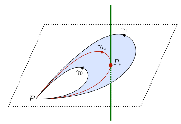
Figure 1: A one-parameter family $\gamma_{t}$ of loops based at $P$ interpolates between $\gamma_{0}$ and $\gamma_{1}$ in the 2-plane transverse to a $B$-operator, represented by the thick vertical line. We depict in red the path $\gamma_{t_{*}}$ corresponding to the critical value $t_{*}$ of $t$ for which the loop hits the $B$-operator.

As before, we use the notation $\Gamma(\gamma_{t})_{0}^{s}$ for the parallel transport along $\gamma_{t}$ from the point $s=0$ to the point with parameter $s$. We recall that the holonomy of a flat connection along a homotopically trivial loop is trivial, hence $\Gamma(\gamma_{0})_{0}^{1}=1$. Next, we apply the non-Abelian Stokes’ formula (19). As we vary $(s,t)$ parametrizing the surface swept by the 1-parameter family of loops $\gamma_{t}(s)$, $F_{\mu\nu}(x(s,t))$ is everywhere zero, except for a single point $(s_{*},t_{*})$. Indeed, there is a unique value $t_{*}\in(0,1)$ of $t$ such that the loop $\gamma_{t_{*}}$ touches the support $\Sigma^{d-1}$ of the $B$-operator; we use $s_{*}$ to denote the value of the $s$ parameter along the loop $\gamma_{t_{*}}(s)$ such that $\gamma_{t_{*}}(s_{*})$ is the point of contact with $\Sigma^{d-1}$. In other words, $F_{\mu\nu}(s,t)$ in (19) is proportional to $\delta(s-s_{*})\delta(t-t_{*})$. The factor $\delta(s-s_{*})$ allows us to do immediately the integral in the variable $s$. We are left with the following result,

$$\Big(\Gamma(\gamma_{t})_{0}^{1}\Big)^{-1}\frac{\partial\Gamma(\gamma_{t})_{0}^{1}}{\partial t}=2\pi\delta(t-t_{*})\Big(\Gamma(\gamma_{t_{*}})_{0}^{s_{*}}\Big)^{-1}U(x(s_{*},t_{*}))X_{0}U(x(s_{*},t_{*}))^{-1}\Gamma(\gamma_{t_{*}})_{0}^{s_{*}}\ .$$ (38)

We notice that the RHS is $\delta(t-t_{*})$ times a $t$-independent element in $\mathfrak{g}$. This suggests the parametrization

$$\Gamma(\gamma_{t})_{0}^{1}=\exp(f(t)Y)\ ,$$ (39)

for some function $f(t)$ and some constant $Y\in\mathfrak{g}$. Then, $(\Gamma(\gamma_{t})_{0}^{1})^{-1}\partial_{t}\Gamma(\gamma_{t})_{0}^{1}=\partial_{t}fY$. We can satisfy (38) together with the boundary condition $\Gamma(\gamma_{0})_{0}^{1}=1$ if we select

$$f(t)=\theta(t-t_{*})\ ,\qquad Y=2\pi\Big(\Gamma(\gamma_{t_{*}})_{0}^{s_{*}}\Big)^{-1}U(x(s_{*},t_{*}))X_{0}U(x(s_{*},t_{*}))^{-1}\Gamma(\gamma_{t_{*}})_{0}^{s_{*}}\ .$$ (40)

where $\theta$ is the Heaviside theta function. With these identifications we conclude that

$$\Gamma(\gamma_{t})_{0}^{1} =1\ , t<t_{*}\ ,$$ (41)

$$\Gamma(\gamma_{t})_{0}^{1} =\Big(\Gamma(\gamma_{t_{*}})_{0}^{s_{*}}\Big)^{-1}U(x(s_{*},t_{*}))e^{2\pi X_{0}}U(x(s_{*},t_{*}))^{-1}\Gamma(\gamma_{t_{*}})_{0}^{s_{*}}\ , t>t_{*}\ .$$

We have recalled $e^{gXg^{-1}}=ge^{X}g^{-1}$ for any $g\in G$, $X\in\mathfrak{g}$. The second line encodes the desired result, but we can formulate it in a more transparent way by introducing a more convenient notation. First, let us write

$$\Gamma(\gamma_{t})_{0}^{1}={\rm hol}_{\gamma_{t}}\ ,$$ (42)

in order to emphasize that the parallel transport operator $\Gamma(\gamma_{t})_{0}^{1}$ along the loop $\gamma_{t}$ is the same as the holonomy of the $A$ connection along $\gamma_{t}$. Moreover, let us denote as $P_{*}$ the contact point $\gamma_{t_{*}}(s_{*})$, and let us write

$$\Gamma_{P}^{P_{*}}:=\Gamma(\gamma_{t_{*}})_{0}^{s_{*}}\ .$$ (43)

Here we are using the fact that the connection is flat away from the support of the $B$-operator and hence $\Gamma(\gamma_{t_{*}})_{0}^{s_{*}}$ depends on $P$, $P_{*}$, but does not depend on the specific shape of the portion of path $\gamma_{t_{*}}$ connecting $P$ ($s=0$) to $P_{*}$ ($s=s_{*}$). Finally, let us write

$$U(P_{*})=U(x(s_{*},t_{*}))\ ,$$ (44)

and consider $t=1$. In conclusion, we get the equation

$${\rm hol}_{\gamma_{1}}=(\Gamma_{P}^{P_{*}})^{-1}U(P_{*})e^{2\pi X_{0}}U(P_{*})^{-1}\Gamma_{P}^{P_{*}}\ .$$ (45)

This confirms that inserting the $B$-operator implies that the connection $A$ has a non-trivial holonomy along a loop linking with it,

$${\rm hol}_{\gamma_{1}}\sim e^{2\pi X_{0}}\ ,$$ (46)

where $\sim$ is equality up to $G$-conjugation. This is the defining property of a disorder operator of Gukov-Witten type labeled by the conjugacy class $[e^{2\pi X_{0}}]$.

We recall that for $G$ a connected and compact Lie group, the exponential map $\exp:\mathfrak{g}\rightarrow G$ is surjective. In particular, this implies that any conjugacy class $[g_{0}]$ in $G$ can be written in the form

$$[g_{0}]=[e^{2\pi X_{0}}]\ ,$$ (47)

for some $X_{0}\in\mathfrak{g}$. In fact, $X_{0}$ is only defined up to the adjoint action of $G$. As a result, as already noted above, without loss of generality we can take $X_{0}$ to lie in the fundamental Weyl chamber inside the Cartan subalgebra of $\mathfrak{g}$.

Remark.

In the above derivation we set out to compute the holonomy around the loop $\gamma_{1}$ based at $P$, but the final formula (45) apparently depends on more data, namely the choice of interpolating loops via the point $P_{*}$ where the critical loop $\gamma_{t_{*}}$ meets the $B$-operator. In fact, we can argue that the holonomy of $\gamma$ based at $P$ is independent of this extra data (not merely up to conjugation, which is manifest, but as a $G$-valued object). To see this, we imagine repeating the same computation that led to (45) choosing a different one-parameter family of interpolating loops. In general, we will get an expression of the form

$${\rm hol}_{\gamma_{1}}=(\Gamma_{P}^{P_{*}^{\prime}})^{-1}U(P_{*}^{\prime})e^{2\pi X_{0}}U(P_{*}^{\prime})^{-1}\Gamma_{P}^{P_{*}^{\prime}}\ ,$$ (48)

for some point $P_{*}^{\prime}$ on the $B$-operator. Now, we have argued above that, on the worldvolume of the $B$-operator, the $\beta$ equation of motion and local ${\rm Stab}(X_{0})$ invariance allow us to set $U^{-1}(d+A)U=0$. In other words, $U$ is covariantly constant. This implies that, if we connect $P_{*}$ and $P_{*}^{\prime}$ using a path inside the worldvolume of the $B$-operator, we have the simple relation

$$U(P_{*}^{\prime})=(\Gamma_{P_{*}^{\prime}}^{P_{*}})^{-1}U(P_{*})\ .$$ (49)

Now, we plug (49) inside (48) to arrive at the expression

$${\rm hol}_{\gamma_{1}}=(\Gamma_{P}^{P_{*}^{\prime}})^{-1}(\Gamma_{P_{*}^{\prime}}^{P_{*}})^{-1}U(P_{*})e^{2\pi X_{0}}U(P_{*})\Gamma_{P_{*}^{\prime}}^{P_{*}}\Gamma_{P}^{P_{*}^{\prime}}=(\Gamma_{P}^{P_{*}})^{-1}U(P_{*})e^{2\pi X_{0}}U(P_{*})\Gamma_{P}^{P_{*}}\ ,$$ (50)

which is the same $G$ element as in (45).

2.1.5 Linking factor between $B$-operators and Wilson loops

We have seen above that inserting a $B$-operator with parameter $X_{0}$ induces a non-trivial holonomy (45) for the gauge field $A$ around the $B$-operator. With this result we can immediately write down the linking factor between the $B$-operator and a Wilson loop labeled by an irreducible representation $\mathbf{R}$ of $G$. It reads Cattaneo:2002tk; Heidenreich:2021xpr

$$\langle\mathbf{Q}_{X_{0}}(\Sigma^{d-1})\mathbf{W}_{\mathbf{R}}(\gamma)\rangle=\frac{\chi_{\mathbf{R}}(e^{2\pi X_{0}})}{\chi_{\mathbf{R}}(1)}\langle\mathbf{Q}_{X_{0}}(\Sigma^{d-1})\rangle\langle\mathbf{W}_{\mathbf{R}}(\gamma)\rangle\ ,$$ (51)

where the character $\chi_{\mathbf{R}}$ is defined as

$$\chi_{\mathbf{R}}(g):={\rm Tr}_{\mathbf{R}}(g)\;\;\;\text{for }g\in G\ .$$ (52)

The relation (51) encodes the fact that, if we go from a configuration with $B$-operator and Wilson loop linking, and we transition to a configuration in which they are not linked, we pick up a factor $\chi_{\mathbf{R}}(e^{2\pi X_{0}})/\chi_{\mathbf{R}}(1)$. In this language, trivial linking corresponds to the case $\chi_{\mathbf{R}}(e^{2\pi X_{0}})/\chi_{\mathbf{R}}(1)=1$.

2.1.6 Example: $G=SU(N)$

In this section we consider the example of $G=SU(N)$ and we describe explicit expressions for the parameter $X_{0}$ entering $B$-operators and for the conjugacy class $[e^{2\pi X_{0}}]$.

Conventions.

Our conventions for $G=SU(N)$ are as follows. The Lie algebra $\mathfrak{g}=\mathfrak{su}(N)$ consists of traceless antihermitian matrices. The standard maximal torus $T\subset G$ is comprised of diagonal $SU(N)$ matrices. The corresponding Cartan subalgebra $\mathfrak{t}$ consists of traceless diagonal antihermitian matrices. Any element of $\mathfrak{t}$ can be written as

$$X_{0}=i\,{\rm diag}(a_{1},\dots,a_{N})\ ,\qquad a_{1}+\dots+a_{N}=0\ ,\qquad a_{i}\in\mathbb{R}\ .$$ (53)

Alternatively, we can expand $X_{0}$ onto the basis of $\mathfrak{t}$ provided by the fundamental weights $\omega_{i}$, $i=1,\dots,N-1$,

$$X_{0}=\sum_{i=1}^{N-1}\lambda_{i}\omega_{i}\ ,\qquad\lambda_{i}\in\mathbb{R}\ .$$ (54)

The dictionary between (53) and (54) is encoded in the relations

$$\lambda_{i}=a_{i+1}-a_{i}\ ,\qquad i=1,\dots,N-1\ .$$ (55)

This is equivalent to the following definition of the fundamental weights,

$$\omega_{j}=\frac{1}{iN}{\rm diag}\Big(\underbrace{N-j,\dots,N-j}_{\text{$j$ times}},\underbrace{-j,\dots,-j}_{\text{$N-j$ times}}\Big)\ ,\qquad j=1,\dots,N-1\ .$$ (56)

We take the positive definite Ad-invariant inner product on $\mathfrak{g}$ to be

$$g(X,Y)=-{\rm tr}(XY)\ ,$$ (57)

where on the RHS tr is the trace in the defining representation (trace of $N\times N$ matrices). With this normalization, one can verify

$$g(\omega_{i},\omega_{j})=(A^{-1})_{ij}\ ,\qquad i,j=1,\dots,N-1\ ,$$ (58)

where $A$ is the Cartan matrix of $\mathfrak{su}(N)$ (the square matrix of dimension $N-1$ with $2$’s on the diagonals and $-1$’s right below and above).

The simple roots are

$$\alpha_{i}=\sum_{j=1}^{N-1}A_{ij}\omega_{j}\ ,\qquad i=1,\dots,N-1\ ,\qquad\text{with normalization $g(\alpha_{i},\alpha_{i})=2$}\ .$$ (59)

The Weyl group is generated by reflections with respect to the hyperplanes orthogonal to the simple roots, and is isomorphic to the symmetric group $S_{N}$. In terms of the parameters $a_{i}$, $S_{N}$ acts by permuting $(a_{1},\dots,a_{N})$. By acting with a suitable element of the Weyl group, any element $X_{0}\in\mathfrak{t}$ can be mapped into the fundamental Weyl chamber. The latter can be written in terms of the parametrization (53) as

$$\text{fund.\penalty 10000\ Weyl chamber:}\qquad a_{1}\leq a_{2}\leq\dots\leq a_{N}\ ,\qquad a_{1}+\dots+a_{N}=0\ .$$ (60)

Conjugacy classes and Weyl alcove.

Any element in $G$ is conjugate to an element in $T$. Hence, any conjugacy class in $G$ can be presented as

$$[g]=[e^{2\pi X_{0}}]\ ,\qquad\text{for some $X_{0}\in\mathfrak{t}$}\ .$$ (61)

Generically, there are infinitely many $X_{0}\in\mathfrak{t}$ that yield the same conjugacy class $[e^{2\pi X_{0}}]$. In fact, given

$$X_{0}=i{\rm diag}(a_{1},\dots,a_{N})\ ,\quad\sum_{i=1}^{N}a_{i}=0\ ,\quad X_{0}^{\prime}=i{\rm diag}(a_{1}^{\prime},\dots,a_{N}^{\prime})\ ,\quad\sum_{i=1}^{N}a_{i}^{\prime}=0\ ,$$ (62)

$X_{0}$ and $X_{0}^{\prime}$ yield the same $[e^{2\pi X_{0}}]$ if and only if

$$a^{\prime}_{i}=a_{\sigma(i)}+n_{i}\ ,\qquad i=1,\dots,N\ ,\qquad\text{for some $\sigma\in S_{N}$, $n_{i}\in\mathbb{Z}$}\ .$$ (63)

One can prove that elements $X_{0},X_{0}^{\prime}\in\mathfrak{t}$ satisfy (63) if and only if they are related by an affine reflection $r_{\alpha,k}$, namely, the reflection with respect to a hyperplane of the form

$$H_{\alpha,k}=\{\lambda\in\mathfrak{t}|g(\lambda,\alpha)=k\}\ ,$$ (64)

where $\alpha$ is a root and $k\in\mathbb{Z}$. (The case $k=0$ corresponds to a usual Weyl reflection with respect to the hyperplane orthogonal to the root $\alpha$). The group of reflections $r_{\alpha,k}$ is the affine Weyl group. It is generated by $r_{\alpha_{i},0}$, where $\alpha_{i}$ runs over the simple roots, together with $r_{\theta,1}$, where $\theta$ is the highest root.

Figure 2: The Cartan algebra $\mathfrak{t}$ of $G=SU(2)$. The half-line shaded in blue is the fundamental Weyl chamber. The interval shaded in green is the fundamental Weyl alcove. We include also the fundamental weight $\omega_{1}$. The blue points represent different elements $X_{0}\in\mathfrak{t}$ that yield the same conjugacy class $[e^{2\pi X_{0}}]$. They are all related by affine Weyl reflections, namely reflections with respect to the points $k\omega_{1}$, $k\in\mathbb{Z}$.

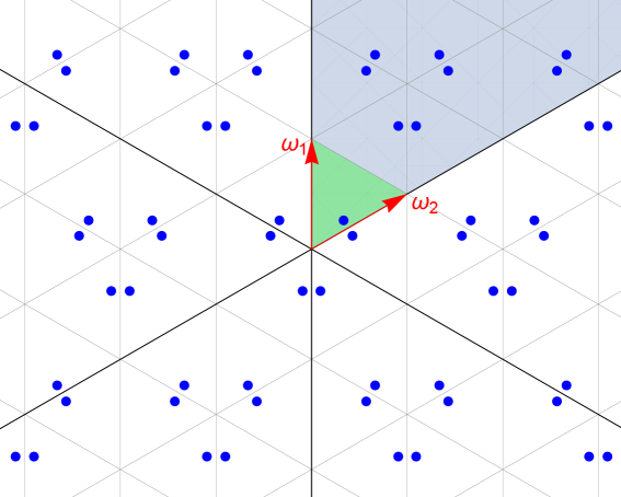
Figure 3: The Cartan algebra $\mathfrak{t}$ of $G=SU(3)$. The unbounded shaded region in blue is the fundamental Weyl chamber. The bounded shaded region in green is the fundamental Weyl alcove. We include also the fundamental weights $\omega_{1}$, $\omega_{2}$. The blue points represent different elements $X_{0}\in\mathfrak{t}$ that yield the same conjugacy class $[e^{2\pi X_{0}}]$. They are all related by affine Weyl reflections, namely reflections with respect to the hyperplanes $H_{\alpha,k}$ as in (64), depicted here as gray and black lines.

A fundamental domain for the action of the affine Weyl group is the fundamental Weyl alcove (of size 1). In terms of the parametrization (53), it is described as

$$\text{fund.\penalty 10000\ Weyl alcove:}\qquad a_{1}\leq a_{2}\leq\dots\leq a_{N}\leq a_{1}+1\ ,\qquad a_{1}+\dots+a_{N}=0\ .$$ (65)

The fundamental Weyl alcove is a bounded subset of the fundamental Weyl chamber.

The notion of Weyl alcove is useful for our discussion because any conjugacy class in $SU(N)$ can be presented in a unique way as

$$[e^{2\pi X_{0}}]\qquad\text{with $X_{0}\in$ fundamental Weyl alcove $\subset\mathfrak{t}$}\ .$$ (66)

We depict the fundamental Weyl chambers and alcoves for $G=SU(2)$ and $G=SU(3)$ in Figures 2 and 3.

2.2 Chern-Simons terms and higher linking

Depending on the gauge group $G$ and the spacetime dimension, one may be able to add extra topological couplings to the BF action (2). In particular, one may add Chern-Simons couplings constructed with the connection 1-form. These additional couplings modify some properties of the $B$-operators of the theory, for example they can induce non-trivial higher-linking correlators. Correspondingly, we shall see that the there can be more information in the label $X_{0}$ of a $B$-operator, than merely the conjugacy class $[e^{2\pi X_{0}}]$ that is detected by linking with Wilson loop operators.

In this section we demonstrate these phenomena with the case study $d=4$, $G=U(1)\times SU(2)$, adding a mixed five-dimensional Chern-Simons term to the BF action. We refer the reader to Antinucci:2024zjp for similar analyses in the Abelian case.

2.2.1 Case study: $d=4$, $G=U(1)\times SU(2)$ with mixed Chern-Simons term

The 5d topological BF action for $G=U(1)\times SU(2)$ can be written in terms of two pairs of fields, $(b,a)$ for the $U(1)$ factor, and $(B,A)$ for the $SU(2)$ factor. More precisely, $b$ is an $\mathbb{R}$-valued 3-form, $a$ is a $U(1)$ connection with field strength $f=da$ whose periods are in $2\pi\mathbb{Z}$. The fields $A$, $B$ are as in Section 2.1.1 with $d=5$, $G=SU(2)$. The action reads

$$S=\int_{X^{5}}\bigg[\frac{1}{2\pi}b\wedge f+\frac{1}{2\pi}{\rm Tr}(B\wedge F_{A})+ka\wedge c_{2}(F_{A})\bigg]\ ,$$ (67)

where $f=da$, $k\in\mathbb{Z}$, and the second Chern form constructed with the $SU(2)$ curvature $F_{A}$ reads

$$c_{2}(F_{A})=\frac{1}{2(2\pi)^{2}}{\rm Tr}(F_{A}\wedge F_{A})\ .$$ (68)

This theory admits topological $b$-operators and $B$-operators,

$$b \mathbf{Q}^{[b]}_{x_{0}}(\Sigma^{3}) \exp\bigg\{ix_{0}\int_{\Sigma^{3}}b\bigg\}\ ,$$-operator : (69)

$$B \mathbf{Q}^{[B]}_{X_{0}}(\Sigma^{3}) \int[\mathcal{D}U][\mathcal{D}\beta] \exp\bigg\{i\int_{\Sigma^{3}}{\rm Tr}\bigg[(B+d_{A}\beta)UX_{0}U^{-1}\bigg]\bigg\}\ ,$$-operator :

where $x_{0}\in\mathbb{R}$ and $X_{0}$ can be taken in the fundamental Weyl chamber of the Cartan algebra of $\mathfrak{su}(2)$. We also have Wilson loop operators for $a$ and $A$,

$$\mathbf{W}^{[a]}_{n}(\gamma)=\exp in\int_{\gamma}a\ ,\qquad{\mathbf{W}}^{[A]}_{\mathbf{R}}(\gamma)={\rm Tr}_{\mathbf{R}}{\rm Pexp}\int_{\gamma}(-A)\ ,$$ (70)

with $n\in\mathbb{Z}$ and $\mathbf{R}$ an irreducible representation of $SU(2)$.

The linking factors of the pairs $(\mathbf{Q}^{[b]}_{x_{0}}(\Sigma^{3}),\mathbf{W}^{[a]}_{n}(\gamma))$ and $(\mathbf{Q}^{[B]}_{X_{0}}(\Sigma^{3}),{\mathbf{W}}^{[A]}_{\mathbf{R}}(\gamma))$ are

$$\langle\mathbf{Q}^{[b]}_{x_{0}}(\Sigma^{3})\mathbf{W}^{[a]}_{\mathbf{R}}(\gamma)\rangle =e^{-2\pi inx_{0}}\langle\mathbf{Q}^{[b]}_{x_{0}}(\Sigma^{3})\rangle\langle\mathbf{W}^{[a]}_{\mathbf{R}}(\gamma)\rangle\ ,$$ (71)

$$\langle\mathbf{Q}^{[B]}_{X_{0}}(\Sigma^{3})\mathbf{W}^{[A]}_{\mathbf{R}}(\gamma)\rangle =\frac{\chi_{\mathbf{R}}(e^{2\pi X_{0}})}{\chi_{\mathbf{R}}(1)}\langle\mathbf{Q}^{[B]}_{X_{0}}(\Sigma^{3})\rangle\langle\mathbf{W}^{[A]}_{\mathbf{R}}(\gamma)\rangle\ .$$

We have assumed that the supports $\Sigma^{3}$, $\gamma$ have linking number one in $X^{5}$.

We now turn to an example of higher linking which detects the level $k$ of the Chern-Simons term in (67). To this end, we insert the operator $\mathbf{Q}^{[B]}_{X_{0}}(\Sigma^{3})$ and we consider the equations of motion of the bulk plus operator system. In particular, we focus on the $B$ and $a$ equations of motion,

$$F_{A}+2\pi UX_{0}U^{-1}\delta_{2}(\Sigma^{3})=0\ ,\qquad db+2\pi kc_{2}(F_{A})=0\ .$$ (72)

These relations together with (68) imply

$$db=-2\pi k\tfrac{1}{2}{\rm Tr}(X_{0}^{2})\delta_{4}(\mathcal{C}^{1})\ ,\qquad\delta_{4}(\mathcal{C}^{1}):=\delta_{2}(\Sigma^{3})\wedge\delta_{2}(\Sigma^{3})\ .$$ (73)

Here we interpret $\delta_{2}(\Sigma^{3})\wedge\delta_{2}(\Sigma^{3})$ as describing the Poincaré dual to the self-intersection $\mathcal{C}^{1}=\Sigma^{3}\cap\Sigma^{3}$. We observe that, for non-zero $k$, the insertion of the operator $\mathbf{Q}^{[B]}_{X_{0}}(\Sigma^{3})$ induces a source for the field $b$. We can probe it by introducing an operator $\mathbf{Q}^{[b]}_{x_{0}}(\widetilde{\Sigma}^{3})$. More precisely, we choose $\widetilde{\Sigma}^{3}=\partial\mathcal{B}^{4}$, with $\mathcal{B}^{4}$ a small 4-disk intersecting $\mathcal{C}^{1}$ once transversely. In other words, $\widetilde{\Sigma}^{3}$ has linking number one with the self-intersection $\mathcal{C}^{1}$. By an application of the usual Stokes’ theorem, the action for the operator $\mathbf{Q}^{[b]}_{x_{0}}(\widetilde{\Sigma}^{3})$ in the background sourced by $\mathbf{Q}^{[B]}_{X_{0}}(\Sigma^{3})$ reads

$$\int_{\widetilde{\Sigma}^{3}}x_{0}b=\int_{\mathcal{B}^{4}}x_{0}db=-2\pi k\tfrac{1}{2}x_{0}{\rm Tr}(X_{0}^{2})\int_{\mathcal{B}^{4}}\delta_{4}(\mathcal{C}^{1})=-2\pi k\tfrac{1}{2}x_{0}{\rm Tr}(X_{0}^{2})\ .$$ (74)

In conclusion, for non-zero $k$ we have a non-trivial higher linking involving the self-intersection of a $B$-operator and a $b$-operator, with linking factor

$$\begin{array}[]{l}\text{$\mathbf{Q}^{[b]}_{x_{0}}(\widetilde{\Sigma}^{3})$, $\mathbf{Q}^{[B]}_{X_{0}}(\Sigma^{3})$,}\\ \text{$\widetilde{\Sigma}^{3}$ links self-intersection of $\Sigma^{3}$:}\end{array}\qquad\exp\Big[-2\pi ik\tfrac{1}{2}x_{0}{\rm Tr}(X_{0}^{2})\Big]\ .$$ (75)

As a small sanity check, we recall that the label $X_{0}$ of the $B$-operator is only defined up to the adjoint action of $SU(2)$. The trace in (75) is indeed invariant under $X_{0}\mapsto gX_{0}g^{-1}$.

Further comments on the labels of $B$- and $b$-operators is in order. If we probe a $b$-operator by linking it with an $a$ Wilson line of arbitrary charge $n$, the result depends on the label $x_{0}$ of the $b$-operator only up to a shift $x_{0}\sim x_{0}+1$, namely only via $e^{2\pi ix_{0}}$. Similarly, if we probe a $B$-operator by linking it with an $A$ Wilson line in an arbitrary irrep $\mathbf{R}$, the result depends on the label $X_{0}$ of the $B$-operator only via the conjugacy class $[e^{2\pi X_{0}}]$. In contrast, for non-zero $k$ the expression (75) for the higher linking depends on $x_{0}$, $X_{0}$, and not only on $e^{2\pi ix_{0}}$ and $[e^{2\pi X_{0}}]$.

One may wonder if we can also have a higher linking involving two distinct $B$-operators, and one $b$-operator. Let us retrace the above steps in this case. Suppose we insert the operators $\mathbf{Q}^{[B]}_{X_{0}^{(1)}}(\Sigma^{3}_{(1)})$ and $\mathbf{Q}^{[B]}_{X_{0}^{(2)}}(\Sigma^{3}_{(2)})$. By reasoning as above, we see that for non-zero $k$ the quantity $db$ contains a source term of the form

$$db\supset-2\pi k{\rm Tr}\Big\{(U_{(1)}X_{0}^{(1)}U_{(1)}^{-1}U_{(2)}X_{0}^{(2)}U_{(2)}^{-1}\Big\}\delta_{2}(\Sigma^{3}_{(1)})\wedge\delta_{2}(\Sigma^{3}_{(2)})\ .$$ (76)

Here $U_{(i)}$, $i=1,2$ are the two independent $SU(2)$-valued 0-forms on the two $B$-operators. Following the same steps from (73) to (75), we infer a linking factor

$$e^{ix_{0}\int_{\mathcal{B}^{4}}db}=\exp\Big[-2\pi ikx_{0}{\rm Tr}\Big\{X_{0}^{(1)}\mathcal{U}X_{0}^{(2)}\mathcal{U}^{-1}\Big\}\Big]\ .$$ (77)

In the last step we have defined $\mathcal{U}=U_{(1)}^{-1}U_{(2)}$. The fields $U_{(i)}$ are integrated over. Recall that in the worldvolume theory of a $B$-operator we can take $U_{(i)}$ to be covariantly constant. The path integral over $U_{(i)}$ reduces effectively to a finite-dimensional integral over $SU(2)$ with the Haar measure. For this reason, the final expression for the sought-for triple linking factor is the average of (77) in $\mathcal{U}$,

$$\begin{array}[]{l}\text{$\mathbf{Q}^{[b]}_{x_{0}}(\widetilde{\Sigma}^{3})$, $\mathbf{Q}^{[B]}_{X_{0}^{(1)}}(\Sigma^{3}_{(1)})$, $\mathbf{Q}^{[B]}_{X_{0}^{(2)}}(\Sigma^{3}_{(2)})$,}\\ \text{$\widetilde{\Sigma}^{3}$ links intersection $\Sigma^{3}_{(1)}\cap\Sigma^{3}_{(2)}$:}\end{array}\qquad\int_{SU(2)}d\mu(\mathcal{U})\exp\Big[-2\pi ikx_{0}{\rm Tr}\Big\{X_{0}^{(1)}\mathcal{U}X_{0}^{(2)}\mathcal{U}^{-1}\Big\}\Big]\ .$$ (78)

Since the labels $X_{0}^{(i)}$ are only defined up to adjoint action, the linking factor ought to be invariant under $X_{0}^{(i)}\mapsto g_{(i)}X_{0}^{(i)}g_{(i)}^{-1}$ with constant $g_{(i)}\in SU(2)$. This is indeed the case, thanks to the fact that we are averaging over $\mathcal{U}$ with a left- and right-invariant measure.

We may say that the effects of the two $B$-operators combine coherently in the terminology introduced in Alford:1992yx for the discussion of non-Abelian vortices.

Finally, let us provide more explicit expressions for the results (75), (78). We set

$$X_{0}=i{\rm diag}(a,-a)\ ,\qquad X_{0}^{(1)}=i{\rm diag}(a^{(1)},-a^{(1)})\ ,\qquad X_{0}^{(2)}=i{\rm diag}(a^{(2)},-a^{(2)})\ .$$ (79)

A generic element of $SU(2)$ is parametrized as

$$\mathcal{U}=\exp(i\tfrac{1}{2}\psi\sigma_{3})\exp(i\tfrac{1}{2}\theta\sigma_{1})\exp(i\tfrac{1}{2}\phi\sigma_{3})\ ,$$ (80)

with $\theta\in[0,\pi]$, $\phi\sim\phi+2\pi$, $\psi\sim\psi+4\pi$. The Haar measure is the (normalized) measure induced by the bi-invariant metric on $SU(2)$, namely the round metric on the 3-sphere,

$$ds^{2}=-\frac{1}{2}{\rm Tr}((\mathcal{U}^{-1}d\mathcal{U})^{2})=\frac{1}{4}(d\theta^{2}+\sin^{2}\theta d\phi^{2})+\frac{1}{4}D\psi^{2}\ ,\qquad D\psi=d\psi+\cos\theta d\phi\ .$$ (81)

With this notation, we compute

$$\exp\Big[-2\pi ik\tfrac{1}{2}x_{0}{\rm Tr}(X_{0}^{2})\Big] =e^{2\pi ikx_{0}a^{2}}\ ,$$ (82)

$$\int_{SU(2)}d\mu(\mathcal{U})\exp\Big[-2\pi ikx_{0}{\rm Tr}\Big\{X_{0}^{(1)}\mathcal{U}X_{0}^{(2)}\mathcal{U}^{-1}\Big\}\Big] =\frac{\sin(4\pi kx_{0}a^{(1)}a^{(2)})}{4\pi kx_{0}a^{(1)}a^{(2)}}\ .$$

These expressions pass a couple of simple consistency checks. First, they are invariant under a sign flip of $a$, $a^{(1)}$, and/or $a^{(2)}$. (These sign flips are the action of the Weyl group $\mathbb{Z}_{2}$ of $SU(2)$ on the $a$ parameters.) Secondly, these linking factors approach 1 if we send any of the parameters $x_{0}$, $a$, $a^{(1)}$, or $a^{(2)}$ to zero.

2.3 Topological operators in the sandwich construction

The $B$-operators and the Wilson loops discussed in the previous section can be formulated without making assumptions on the spacetime $X^{d+1}$. In this section we discuss some additional operators that can be defined when we take $X^{d+1}$ to be the product of a $d$-manifold $M^{d}$ with an interval, $X^{d+1}=M^{d}\times[z_{0},z_{1}]$. The boundary component of $X^{d+1}$ at $z=z_{0}$ is identified with the symmetry boundary of the sandwich construction. On this component, we impose the Dirichlet boundary condition

$$A\Big|_{M^{d}\times\{z_{0}\}}=0\ .$$ (83)

Correspondingly, we restrict the parameter $g$ of bulk gauge transformations (4) to be trivial at the symmetry boundary. The boundary component of $X^{d+1}$ at $z=z_{1}$ is identified with the physical boundary.

2.3.1 Stretched Wilson line operators

A simple class of operators that can be defined on $X^{d+1}=M^{d}\times[z_{0},z_{1}]$ are open Wilson line operators labeled by an irreducible representation $\mathbf{R}$ and stretching along the interval direction $z$. This operator is constructed with the the parallel transport $\Gamma(\gamma)_{0}^{1}$ along a path $\gamma$ connecting a point $Q$ on the physical boundary to a point $P$ on the symmetry boundary,

$$\gamma:[0,1]\rightarrow X^{d+1}\ ,\qquad\gamma(0)=Q\in M^{d}\times\{z_{1}\}\ ,\qquad\gamma(1)=P\in M^{d}\times\{z_{0}\}\ ,$$ (84)

$$\text{(open Wilson line in irrep $\mathbf{R}$)}=\mathbf{W}_{\mathbf{R}}^{o}(\gamma)=D_{\mathbf{R}}(\Gamma(\gamma)_{0}^{1})\ .$$ (85)

Here the symbol $D_{\mathbf{R}}(g)$ denotes the linear map that represents the abstract group element $g\in G$ in the irrep $\mathbf{R}$. The operator $\mathbf{W}_{\mathbf{R}}^{o}(\gamma)$ (where ‘o’ stands for open) is matrix-valued, whereas its closed loop counterpart $\mathbf{W}_{\mathbf{R}}(\gamma)$ is real-valued. Under a gauge transformation,

$$\mathbf{W}_{\mathbf{R}}^{o}(\gamma)\mapsto\mathbf{W}_{\mathbf{R}}^{o}(\gamma)D_{\mathbf{R}}(g(Q)^{-1})\ ,$$ (86)

where we have used $g(P)=1$, hence $D_{\mathbf{R}}(g(P))=\mathbb{I}$, because $P$ lies on the symmetry boundary. The term $D_{\mathbf{R}}(g(Q)^{-1})$ in the gauge variation of $\mathbf{W}_{\mathbf{R}}^{o}(\gamma)$ is compensated by the non-topological endpoint on the physical boundary. Alternatively, we may consider a quiche-like configuration, in which the physical boundary at $z_{1}$ is pushed to infinity and $g(Q)=1$.

Since the connection $A$ is flat in the bulk (away from operator insertions), we already know that $\mathbf{W}_{\mathbf{R}}^{o}(\gamma)$ is invariant under small deformations of the path $\gamma$ that leave the endpoints $P$, $Q$ fixed. Moreover, $\mathbf{W}_{\mathbf{R}}^{o}(\gamma)$ is invariant if we move the point $P$ on the symmetry boundary. More precisely, let us consider a different path $\gamma^{\prime}$ connecting the same $Q$ on the physical boundary to some $P^{\prime}$ on the symmetry boundary. We can smoothly deform $\gamma^{\prime}$ to a path $\gamma^{\prime\prime}$ that first connects $Q$ to $P$ along the original path $\gamma$, and then $P$ to $P^{\prime}$ along the symmetry boundary The only potential difference in the final result can originate from the portion of the path $\gamma^{\prime\prime}$ connecting $P$ to $P^{\prime}$. But on the physical boundary the connection is identically zero due to the Dirichlet boundary condition, ensuring that parallel transport along any path inside the symmetry boundary is trivial. We then conclude that $\mathbf{W}_{\mathbf{R}}^{o}(\gamma)$ is invariant if we deform $\gamma$ and/or move the point $P$. In contrast, the operator is not invariant if we move the point $Q$ on the physical boundary. Indeed, upon closing the sandwich, $\mathbf{W}_{\mathbf{R}}^{o}(\gamma)$ yields a non-topological local operator in the QFT $\mathcal{T}$.

2.3.2 Non-genuine $B$-operators

Let us now discuss a different version of $B$-operators, that are non-genuine. More precisely, they are defined on $d$-dimensional cylinder $\Sigma^{d-1}\times[z_{0},z_{*}]$, where $\Sigma^{d-1}$ is a cycle in $M^{d}$ and $z_{*}\in(z_{0},z_{1})$ is a fixed value along the interval direction, see Figure 4.

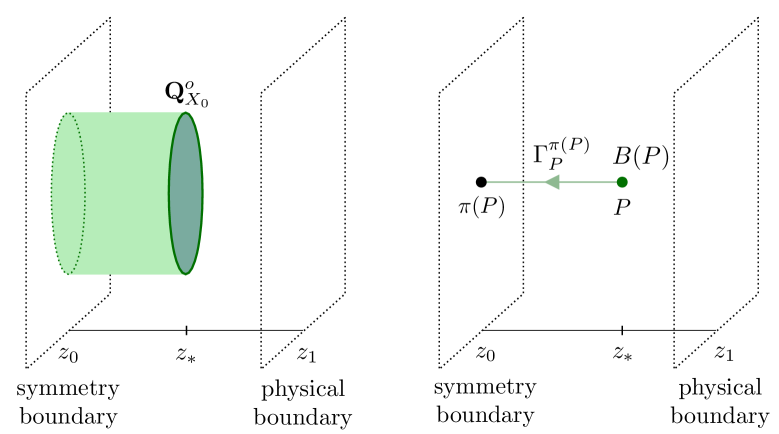
Figure 4: On the left: The non-genuine $B$-operator $\mathbf{Q}^{o}_{X_{0}}$ is supported on the cyclinder $\Sigma^{d-1}\times[z_{0},z_{*}]$. It is constructed by integrating the dressed $\mathcal{B}$ operator (87). On the right: the dressed operator $\mathcal{B}$ is defined combining the field $B$ at the point $P$ with the parallel transport operator along a segment connecting $P$ to its projection $\pi(P)$ onto the symmetry boundary.

We start with a preliminary definition. Let $P$ be a point in the interior of $X^{d+1}=M^{d}\times[z_{0},z_{1}]$, sitting at a value $z_{*}$ of the interval coordinate and a value $x$ for coordinates on $M^{d}$. Consider the path connecting the point $P$ to its projection $\pi(P)$ onto the symmetry boundary, which in coordinates has the same value $x$ as $P$, but $z=z_{0}$. We multiply the field $B$ at the point $P$ by the parallel transport operator from $P$ to $\pi(P)$ along a straight path stretching in the interval direction, see Figure 4. In this way we define a dressed version of $B$, denoted $\mathcal{B}$,

$$\mathcal{\mathcal{B}}(P)=\Gamma_{P}^{\pi(P)}B(P)(\Gamma_{P}^{\pi(P)})^{-1}\ .$$ (87)

We are using the compact notation $\Gamma_{P}^{\pi(P)}$ for the parallel transport from $P$ to $\pi(P)$. Under a bulk gauge transformation (4),

$$A\mapsto g(d+A)g^{-1}\ ,\qquad B\mapsto g(B-d_{A}\tau)g^{-1}\ ,\qquad\Gamma_{P}^{\pi(P)}\mapsto g(\pi(P))\Gamma_{P}^{\pi(P)}g(P)^{-1}\ .$$ (88)

Notice, however, that $g(\pi(P))=1$ because $\pi(P)$ lies on the symmetry boundary. As a result, we have

$$\mathcal{\mathcal{B}}(P)\mapsto\mathcal{\mathcal{B}}(P)-\Gamma_{P}^{\pi(P)}(d_{A}\tau)(P)(\Gamma_{P}^{\pi(P)})^{-1}\ .$$ (89)

Next, we use the dressed operator $\mathcal{B}$ to construct a non-genuine version of a $B$-operator. This is achieved by integrating $\mathcal{B}$ on $\Sigma^{d-1}\times\{z_{*}\}$. Each point $P$ on $\Sigma^{d-1}\times\{z_{*}\}$ comes with its interval attaching it to $\pi(P)$, so that result of the integration is not a genuine operator on $\Sigma^{d-1}\times\{z_{*}\}$, but rather an operator on the cylinder $\Sigma^{d-1}\times[z_{0},z_{*}]$, as anticipated. We can write this operator as

$$\mathbf{Q}^{o}_{X_{0}}(\Sigma^{d-1}\times[z_{0},z_{*}])\;:\;\;\exp\bigg\{\frac{i}{2\pi}\int_{P\in\Sigma^{d-1}\times\{z_{*}\}}{\rm Tr}(\mathcal{B}(P)X_{0})\bigg\}\ .$$ (90)

We may contrast this operator with the genuine $B$-operator in (20). We notice that the definition of $\mathbf{Q}^{o}_{X_{0}}$ does not require localized fields, in contrast to the fields $U$, $\beta$ in (20). Indeed, the expression in (90) is gauge invariant without the need of any additional compensating local fields. This follows from (89) and the identity

$$\Gamma_{P}^{\pi(P)}(d_{A}\tau)(P)(\Gamma_{P}^{\pi(P)})^{-1}=d\Big[\Gamma_{P}^{\pi(P)}\tau(P)(\Gamma_{P}^{\pi(P)})^{-1}]\ .$$ (91)

This identity ensures that the $d_{A}\tau$ shift in (89) yields a total derivative in the integrand of (90). It can be derived following steps analogous to those leading to the non-Abelian Stokes’ formula (19), using flatness of the connection.

We stress that $\mathbf{Q}^{o}_{X_{0}}$ depends on $X_{0}\in\mathfrak{g}$, while its genuine counterpart $\mathbf{Q}_{X_{0}}$ depends on $X_{0}\in\mathfrak{g}$ only up to the adjoint action of $G$ on $\mathfrak{g}$.

Operators restricted on the boundary.

Finally, we may also consider the limit in which the position $z_{*}$ along the interval direction approaches the value $z_{0}$ of the symmetry boundary. In this limit, the operator $\mathbf{Q}^{o}_{X_{0}}$ yields a genuine operator, albeit one that is restricted to lie inside the symmetry boundary. We denote this operator as

$$D_{X_{0}}(\Sigma^{d-1}\times\{z_{0}\})=\lim_{z_{*}\rightarrow z_{0}}\mathbf{Q}^{o}_{X_{0}}(\Sigma^{d-1}\times[z_{0},z_{*}])\ .$$ (92)

Comparing with (90), we see that this operator can be described by the exponentiated action

$$\exp\bigg\{\frac{i}{2\pi}\int_{P\in\Sigma^{d-1}\times\{z_{*}\}}{\rm Tr}(BX_{0})\bigg\}\ .$$ (93)

The presentation (92) will be useful below in discussing linking with Wilson lines.

Linking with Wilson lines.

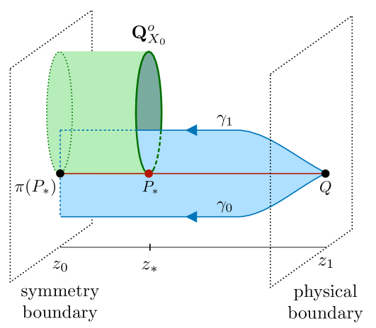
Figure 5: A one-parameter family of Wilson paths sweeps a surface intersecting a non-genuine $B$-operator on $\Sigma^{d-1}\times[z_{0},z_{*}]$. The point $P_{*}$ is the intersection of the surface swept by the one-parameter family of paths and $\Sigma^{d-1}\times\{z_{*}\}$.

Next, let us consider the linking factor between a non-genuine $B$-operator and a stretched Wilson line operator. We can analyze this linking by deforming the path of the Wilson line and applying the non-Abelian Stokes’ formula, see Figure 5. More precisely, we consider a one-parameter family $\gamma_{t}$ of paths with

$$t\in[0,1]\ ,\quad s\in[0,1]\ ,\quad\gamma_{t}(0)=Q\ ,\qquad\gamma_{t}(1)=P_{t}\ ,$$ (94)

where $Q$ is on the physical boundary, $P_{t}$ is on the symmetry boundary. The surface swept by this one-parameter family of paths intersects the support of the non-genuine $B$-operator at the point $P_{*}$, corresponding to values $t_{*}$, $s_{*}$ of the $t$, $s$ parameters. Without loss of generality, we can arrange the one-parameter family in such a way that the projection $\pi(P_{*})$ of $P_{*}$ onto the symmetry boundary is the same as the endpoint $P_{t_{*}}$ of the path $\gamma_{t_{*}}$.

After these preliminaries, we apply the non-Abelian Stokes’ formula (19). (We get no contribution from the variation of the endpoint $P_{t}$ on the symmetry boundary because the connection is zero there.) We get a non-zero contribution from a localized field strength,

$$F_{A}+(\Gamma_{P_{*}}^{\pi(P_{*})})^{-1}X_{0}\Gamma_{P_{*}}^{\pi(P_{*})}\delta_{1}(\Sigma^{d-1}\subset M^{d})\delta(z-z_{*})dz=0\ ,$$ (95)

as follows from the variation of the total action (2) plus (90) with respect to $B$. Plugging this field strength into (19) we get the equation

$$\Big(\Gamma(\gamma_{t})_{0}^{1}\Big)^{-1}\frac{\partial\Gamma(\gamma_{t})_{0}^{1}}{\partial t}=\delta(t-t_{*})\Big(\Gamma(\gamma_{t_{*}})_{0}^{s_{*}}\Big)^{-1}(\Gamma_{P_{*}}^{\pi(P_{*})})^{-1}X_{0}\Gamma_{P_{*}}^{\pi(P_{*})}\Gamma(\gamma_{t_{*}})_{0}^{s_{*}}\ .$$ (96)

We observe that the product $\Gamma_{P_{*}}^{\pi(P_{*})}\Gamma(\gamma_{t_{*}})_{0}^{s_{*}}$ amounts to parallel transport from the starting point $Q$ at $s=0$, to the contact point $P_{*}$ at $s=s_{*}$, followed by transport from $P_{*}$ to $\pi(P_{*})$. All in all, this is equal to $\Gamma(\gamma_{t_{*}})_{0}^{1}$. (Here we are using the fact the connection is flat away from $P_{*}$ and hence parallel transport depends on the initial and final points, but not on the specific shape of the path connecting them. Moreover, we recall that the endpoint $\gamma_{t_{*}}(1)$ is the same as $\pi(P_{*})$.) The above remarks shows that we can recast (96) in the form

$$\Big(\Gamma(\gamma_{t})_{0}^{1}\Big)^{-1}\frac{\partial\Gamma(\gamma_{t})_{0}^{1}}{\partial t}=\delta(t-t_{*})\Big(\Gamma(\gamma_{t_{*}})_{0}^{1}\Big)^{-1}X_{0}\Gamma(\gamma_{t_{*}})_{0}^{1}\ ,$$ (97)

or equivalently

$$\bigg[\Gamma(\gamma_{t})_{0}^{1}\Big(\Gamma(\gamma_{t_{*}})_{0}^{1}\Big)^{-1}\bigg]^{-1}\frac{\partial}{\partial t}\bigg[\Gamma(\gamma_{t})_{0}^{1}\Big(\Gamma(\gamma_{t_{*}})_{0}^{1}\Big)^{-1}\bigg]=\delta(t-t_{*})X_{0}\ .$$ (98)

Since the RHS is of the form $\delta(t-t_{*})$ times a constant element of $\mathfrak{g}$, we adopt the parametrization

$$\Gamma(\gamma_{t})_{0}^{1}\Big(\Gamma(\gamma_{t_{*}})_{0}^{1}\Big)^{-1}=\exp(f(t)X_{0})\ ,$$ (99)

where $f(t)$ is a scalar function of $t$. We see that, if we choose $f(t)=\theta(t-t_{*})$, we satisfy (98), as well as the consistency requirement $\Gamma(\gamma_{t})_{0}^{1}\Big(\Gamma(\gamma_{t_{*}})_{0}^{1}\Big)^{-1}=1$ for $t=t_{*}$. In conclusion,

$$\Gamma(\gamma_{t})_{0}^{1} =\Gamma(\gamma_{t_{*}})_{0}^{1}\ , t\leq t_{*}\ ,$$ (100)

$$\Gamma(\gamma_{t})_{0}^{1} =e^{X_{0}}\Gamma(\gamma_{t_{*}})_{0}^{1}\ , t>t_{*}\ .$$

In other words, upon sweeping the path across the $B$-surface, the value of parallel transport is multiplied on the left by $e^{X}_{0}\in G$. With this result we can immediately write down the effect of passing a non-genuine $B$-operator past a stretched Wilson line,

$$\text{swipe $\mathbf{Q}^{o}_{X_{0}}$ through $\mathbf{W}_{\mathbf{R}}^{o}$:}\qquad\mathbf{W}_{\mathbf{R}}^{o}(\gamma)\mapsto D_{\mathbf{R}}(e^{X_{0}})\mathbf{W}_{\mathbf{R}}^{o}(\gamma)\ .$$ (101)

Recall that $D_{\mathbf{R}}$ is the map that associates to an element of $G$ the matrix that represents it in the irrep $\mathbf{R}$.

It is straightforward to specialize the above results to the limit $z_{*}\rightarrow z_{0}$, in which the non-genuine operator $\mathbf{Q}_{X_{0}}(\Sigma^{d-1}\times[z_{0},z_{*}])$ yields the genuine operator $D_{X_{0}}(\Sigma^{d-1}\times\{z_{0}\})$ stuck at the symmetry boundary. In particular, (101) implies that passing an $D_{X_{0}}$ operator past a stretched Wilson line has the effect

$$\text{swipe $D_{X_{0}}$ through $\mathbf{W}_{\mathbf{R}}^{o}$:}\qquad\mathbf{W}_{\mathbf{R}}^{o}(\gamma)\mapsto D_{\mathbf{R}}(e^{X_{0}})\mathbf{W}_{\mathbf{R}}^{o}(\gamma)\ .$$ (102)

The operator $D_{X_{0}}(\Sigma^{d-1}\times\{z_{0}\})$ provides an explicit realization of a class of operators discussed in Bonetti:2024cjk, see also Jia:2025jmn. These operators are stuck on the symmetry boundary and are labeled by a group element (here $e^{X_{0}}$), as opposed to a conjugacy class. They act on stretched Wilson lines as in (102).

2.4 Some remarks on fusion

In this subsection we comment on some aspects of the fusion of topological operators of the bulk SymTFT described by (2).

2.4.1 Wilson line operators

For any $d$, the bulk $(d+1)$-dimensional BF theory (2) admits simple topological Wilson line operators labeled by irreducible representations of the group $G$, which is a compact Lie group. They close under fusion. Indeed, they fuse according to the tensor product of the representations that label them. In other words, the bulk $(d+1)$-dimensional topological theory contains a set of topological line operators described by the category ${\rm Rep}(G)$.

2.4.2 Observations on the fusion of $B$-defects

In this work we do not address systematically the fusion of $B$-defects in the bulk $(d+1)$-dimensional BF theory (2). To gain some preliminary intuition, however, we can first revisit the case of $G$ a finite non-Abelian group.

Finite non-Abelian group.

Let us consider a $(d+1)$-dimensional Dijkgraaf-Witten theory Dijkgraaf:1989pz with gauge group $G$. For simplicity, we restrict ourselves to the case of trivial cocycle. The theory contains topological codimension-two operators labeled by a conjugacy class $C$ in $G$, which we denote $D_{d-1}^{(C)}$. They can be thought of as Gukov-Witten operators, in the sense that inserting $D_{d-1}^{(C)}$ on $\Sigma^{d-1}$ amounts to imposing a holonomy for the (flat) discrete $G$ gauge field around $\Sigma^{d-1}$, given up to conjugation by the class $C$. We regard the operators $D_{d-1}^{(C)}$ as the finite-group analog of the $B$-defects studied earlier in this work.

Let us recall some properties of the fusion of the topological operators $D_{d-1}^{(C)}$, following Dijkgraaf:1989hb. The operator $D_{d-1}^{(C_{3})}$ is an allowed fusion channel in $D_{d-1}^{(C_{1})}\otimes D_{d-1}^{(C_{2})}$ if there exist $g_{1}\in C_{1}$, $g_{2}\in C_{2}$ such that $g_{1}g_{2}\in C_{3}$. More precisely, we can write

$$D_{d-1}^{(C_{1})}\otimes D_{d-1}^{(C_{2})}=\sum_{C_{3}}N_{C_{1}C_{2}}{}^{C_{3}}D_{d-1}^{(C_{3})}+\dots$$ (103)

The fusion coefficient $N_{C_{1}C_{2}}{}^{C_{3}}$ is the number of $G$-orbits in the set

$$\{(g_{1},g_{2},g_{3})\in C_{1}\times C_{2}\times C_{3}|g_{1}g_{2}=g_{3}\}\ ,$$ (104)

where $G$ acts on triples $(g_{1},g_{2},g_{3})$ by simultaneous conjugation.

The ellipses on the RHS of (103) indicate that generically we expect additional contributions in the fusion rule. To clarify this point we can focus on the case $d=2$. The 3d bulk topological theory admits simple line operators labeled by pairs $(C,\pi)$, where $C$ is a conjugacy class of $G$ and $\pi$ is an irreducible representation of the centralizer subgroup $N_{g}$ of $g\in C$. (Different choices of representatives $g\in C$ is give isomorphic centralizer subgroups.) Heuristically, we can think of the topological line labeled $(C,\pi)$ as a “pure” Gukov-Witten operator with label $C$ stacked with a Wilson line in the representation $\pi$ of the “unbroken gauge group” $N_{g}\subset G$ living on the worldvolume of the Gukov-Witten operator. The lines with label $(C=\{e\},\pi)$, namely with trivial conjugacy class, are topological Wilson line operators for the full gauge group $G$ in the 3d bulk.

Let us denote the topological line with label $(C,\pi)$ as $D_{1}^{(C,\pi)}$. The fusion algebra of the operators $D_{1}^{(C,\pi)}$ takes the form

$$D_{1}^{(C_{1},\pi_{1})}\otimes D_{1}^{(C_{2},\pi_{2})}=\sum_{(C_{3},\pi_{3})}N_{(C_{1},\pi_{1})(C_{2},\pi_{2})}{}^{(C_{3},\pi_{3})}D_{1}^{(C_{3},\pi_{3})}\ ,$$ (105)

where the fusion coefficients are known in closed form Dijkgraaf:1989hb; Roche:1990hs. For brevity, we refrain from writing down their expressions. Let us emphasize, however, two salient features of the fusion coefficients.

• If we consider the case in which $\pi_{1}$, $\pi_{2}$, $\pi_{3}$ are the trivial representation (denoted $\mathbf{1}$), then the fusion coefficient $N_{(C_{1},\mathbf{1})(C_{2},\mathbf{1})}{}^{(C_{3},\mathbf{1})}$ equals the fusion coefficient $N_{C_{1}C_{2}}{}^{C_{3}}$ described in (103), (104).

• If $\pi_{1}$ and $\pi_{2}$ are trivial, but $\pi_{3}$ is non-trivial, the fusion coefficient $N_{(C_{1},\mathbf{1})(C_{2},\mathbf{1})}{}^{(C_{3},\pi_{3})}$ can be different from zero. This can be checked, for example, in the case $G=S_{3}$.

The second point shows that the subset of “pure” Gukov-Witten operators with labels $(C,\pi=\mathbf{1})$ does not generically close under fusion. This substantiates the claim made earlier that additional terms are present in (103), besides those written down explicitly. In contrast, one can verify using the expressions of the fusion coefficients $N_{(C_{1},\pi_{1})(C_{2},\pi_{2})}{}^{(C_{3},\pi_{3})}$ that the lines with labels $(C=\{e\},\pi)$ (i.e. Wilson lines) do close under fusion, in accordance with our general claim above.

In categorical language, the topological line operators of the 3d Dijkgraaf-Witten theory with gauge group $G$ form a category, which is the Drinfeld center $\mathcal{Z}({\rm Vec}_{G})$ of ${\rm Vec}_{G}$. The discussion of the previous paragraphs is an informal account of some properties of $\mathcal{Z}({\rm Vec}_{G})$, see e.g. lusztig1984characters; lusztig1987leading, (bakalov2001lectures, Chapter 3), (etingof2015tensor, ex. 8.5.4). In particular, it is known that willerton2008twisted

$$\mathcal{Z}({\rm Vec}_{G})\cong\bigoplus_{[g]}{\rm Rep}(N_{g})\ ,$$ (106)

corresponding to the fact that simple lines in the Drinfeld center are labeled by a conjugacy class $[g]$ and an irreducible representation of the centralizer of $g$. (An analogous statement holds in the twisted case, see e.g. willerton2008twisted.)

An analog of (106) is available in the case $d=3$, namely for a 4d Dijkgraaf-Witten theory. In this case the topological surface operators in the 4d bulk form a 2-category, which is the Drinfeld center $\mathcal{Z}(2{\rm Vec}_{G})$ of the 2-category $2{\rm Vec}_{G}$. One has kong2020center

$$\mathcal{Z}(2{\rm Vec}_{G})\cong\bigoplus_{[g]}2{\rm Rep}(N_{g})\ .$$ (107)

(Once again, for simplicity we restrict to the untwisted case, but analogous results are available with twist.) This encodes the fact that simple topological surface operators in the 4d bulk are labeled by a conjugacy class $[g]$ and an irreducible 2-representation of the centralizer subgroup $N_{g}$. Now, an irreducible 2-representation of $N_{g}$ is labeled by: (i) a subgroup $H$ of $N_{g}$; (ii) a group cohomology class $\psi\in H^{2}(H,\mathbb{C}^{\times})$ ostrik2002module; kong2020center. These data also label irreducible 2d TQFTs with $N_{g}$ non-anomalous 0-form symmetry, see e.g. Bhardwaj:2023ayw. Thus, heuristically, we can think of the topological surface operators in the 4d bulk of the Dijkgraaf-Witten theory as “pure” Gukov-Witten operator labeled by the conjugacy class $[g]$ stacked with a 2d TQFT whose global symmetry equals the “unbroken gauge group” on the worldvolume of the Gukov-Witten operator.

The natural generalization of (106) for $d\geq 4$,

$$\mathcal{Z}((d-1){\rm Vec}_{G})\cong\bigoplus_{[g]}(d-1){\rm Rep}(N_{g})\ ,$$ (108)

has also been put forward in the mathematical literature kong2020center and motivated by physical arguments Bhardwaj:2023ayw. Heuristically, we interpret (108) as the statement that simple codimension-two topological operators in the bulk of the $(d+1)$-dimesional Dijkgraaf-Witten theory with gauge group $G$ are realized by starting from a “pure” Gukov-Witten operator labeled by a conjugacy class $[g]$ and stacking it with a simple $(d-1)$-dimensional TQFT with global symmetry $N_{g}$.

Building on the case $d=2$, we have the following expectations regarding the fusion of codimension-two operators in the $(d+1)$-dimesional Dijkgraaf-Witten theory.

• The fusion of “pure” Gukov-Witten operators follows the pattern (103) with the specified fusion coefficients $N_{C_{1}C_{2}}{}^{C_{3}}$.

• The set of “pure” Gukov-Witten operators may in general not close under fusion.

It would be interesting to test these claims in the case $d=3$, using the explicit fusion rules given in kong2020center, but this goes beyond the scope of this paper.

Continuous non-Abelian group.

The intuition coming from the case of finite non-Abelian group leads us to the following expectations for the fusion of $B$-defects (20) in the case of a compact Lie group $G$.

Recall that the $B$-defect $\mathbf{Q}_{X_{0}}(\Sigma^{d-1})$ is a Gukov-Witten operator inducing a holonomy labeled by the conjugacy class $[e^{2\pi X_{0}}]$. In analogy with (103), (104), we expect that the operator $\mathbf{Q}_{X_{0}^{(3)}}(\Sigma^{d-1})$ is an allowed fusion channel in $\mathbf{Q}_{X_{0}^{(1)}}(\Sigma^{d-1})\otimes\mathbf{Q}_{X_{0}^{(2)}}(\Sigma^{d-1})$ if there exist $g,\ell\in G$ such that

$$e^{2\pi X_{0}^{(1)}}ge^{2\pi X_{0}^{(2)}}g^{-1}=\ell e^{2\pi X_{0}^{(3)}}\ell^{-1}\ .$$ (109)

In particular, for generic $X_{0}^{(1)}$, $X_{0}^{(2)}$ we have a continuum of allowed fusion channels $X_{0}^{(3)}$.

For example, let $G=SU(2)$. As described in Section 2.1.6, without loss of generality the parameters $X_{0}^{(1)}$, $X_{0}^{(2)}$ take the form

$$X_{0}^{(1)}=i\,{\rm diag}(a^{(1)},-a^{(1)})\ ,\qquad-\tfrac{1}{2}\leq a^{(1)}\leq 0\ ,$$ (110)

namely we can take $a^{(1)}$ in the fundamental Weyl alcove, and similarly for $X_{0}^{(2)}$. A generic element $g\in SU(2)$ can be parametrized as

$$g=e^{i\frac{1}{2}\psi\sigma_{3}}e^{i\frac{1}{2}\theta\sigma_{1}}e^{i\frac{1}{2}\phi\sigma_{3}}\ ,\qquad\theta\in[0,\pi]\ ,\quad\phi\in[0,2\pi)\ ,\quad\psi\in[0,4\pi)\ ,$$ (111)

where $\sigma$’s denote the standard Pauli matrices. A direct computation shows that

$$e^{2\pi X_{0}^{(1)}}ge^{2\pi X_{0}^{(2)}}g^{-1}\sim{\rm diag}(e^{2\pi ia^{(3)}},e^{-2\pi ia^{(3)}})\ ,$$ (112)

where $\sim$ denotes equality up to conjugation in $SU(2)$ and $a^{(3)}$ satisfies

$$\cos(2\pi a^{(3)})=\cos(2\pi a^{(1)})\cos(2\pi a^{(2)})-\cos\theta\sin(2\pi a^{(1)})\sin(2\pi a^{(2)})\ .$$ (113)

As $\theta$ varies, we run over the possible fusion channels. The allowed values for $a_{3}$ in the fundamental Weyl alcove are

$$-\tfrac{1}{2}\leq\left|a^{(1)}+a^{(2)}+\tfrac{1}{2}\right|-\tfrac{1}{2}\leq a^{(3)}\leq-|a^{(1)}-a^{(2)}|\leq 0\ .$$ (114)

This proposal for the fusion of $B$-defects differs from analogous proposals, such as the fusion rule of averaged operators in Cordova:2022rer. According to that paper, for $G=SU(2)$ one finds only two fusion channels on the RHS, as opposed to a continuum of possible values. We hope to return to this point in the future to clarify it further.

As a final comment, the intuition from the case of finite $G$ suggests that the fusion of $B$-defects might not be closed. Additional topological operators might have to be included in the fusion algebra, which are the analog of the operators in the Dijkgraaf-Witten theory with a non-trivial (higher) representation label. Conjecturally, they might be obtained from a “pure” $B$-defect as in (20) by stacking a $(d-1)$-dimensional TQFT with global symmetry ${\rm Stab}(X_{0})\subset G$, which corresponds to the “unbroken gauge group” on the worldvolume of the $B$-defect, and performing a (flat) gauging of the diagonal ${\rm Stab}(X_{0})$. Carrying out this construction, however, is beyond the scope of this note.

2.5 Proposal to accommodate non-flat Dirichlet boundary conditions

According to the proposal of Brennan:2024fgj; Antinucci:2024zjp; Bonetti:2024cjk discussed in Section 2, the bulk-boundary description of a continuous global 0-form symmetry $G$ makes use of the topological BF theory (2) with gauge group $G$. This is equipped with Dirichlet boundary conditions for the gauge field $A$ on the symmetry boundary. Due to the bulk equations of motion, the boundary value of $A$ must necessarily be a flat connection. In this section we propose a generalization of the above framework, which allows us to impose Dirichlet boundary conditions with non-flat boundary values for $A$. To achieve this goal, we consider a family of bulk theories on $X^{d+1}$, all based on the same gauge group $G$. A member of the family is determined by a choice of background $G$-connection $\mathcal{A}$ on $X^{d+1}$. The proposed bulk action does not give rise to any propagating degrees of freedom (in contrast, say, to a standard Yang-Mills action).

Action, gauge symmetries, equations of motion.

The dynamical fields on $X^{d+1}$ are: a $G$-connection $A$; a $\mathfrak{g}$-valued $(d-1)$-form $B$; a $\mathfrak{g}$-valued $(d-2)$-form $\beta$; a $G$-valued 0-form $U$. We also need to choose a non-dynamical background $G$-connection $\mathcal{A}$. The action reads

$$S=\frac{1}{2\pi}\int_{X^{d+1}}{\rm Tr}\bigg[(B+d_{A}\beta)\wedge(F_{A}-U\mathcal{F}U^{-1})\bigg]\ .$$ (115)

This action is written in terms of the quantities

$$F_{A}=dA+\tfrac{1}{2}[A,A]\ ,\qquad d_{A}\beta=d\beta+[A,\beta]\ ,\qquad\mathcal{F}=d\mathcal{A}+\tfrac{1}{2}[\mathcal{A},\mathcal{A}]\ .$$ (116)

The action (115) is invariant under

$$A \mapsto g(d+A)g^{-1}\ , B \mapsto g(B-d_{A}\tau)g^{-1}\ , \beta \mapsto g(\beta+\tau)g^{-1}\ ,$$ (117)

$$\mathcal{A} \mapsto\overline{g}(d+\mathcal{A})\overline{g}^{-1}\ , U \mapsto gU\overline{g}^{-1}\ .$$

Here $g$, $\overline{g}$ are a $G$-valued 0-forms, with $g$ the parameter of a gauge transformation of the dynamical $A$, and $\overline{g}$ for $\mathcal{A}$. As usual, $\tau$ is a $\mathfrak{g}$-valued $(d-2)$-form.

The equations of motion for $A$, $B$, $U$, $\beta$ read

$$0 =d_{A}(B+d_{A}\beta)+[\beta,F_{A}-U\mathcal{F}U^{-1}]\ ,$$ (118)

$$0 =F_{A}-U\mathcal{F}U^{-1}\ ,$$

$$0 =[B+d_{A}\beta,U\mathcal{F}U^{-1}]\ ,$$

$$0 =d_{A}(U\mathcal{F}U^{-1})\ ,$$

respectively. We have made use of the Bianchi identity $d_{A}F_{A}=0$ and of $d_{A}d_{A}\beta=[F_{A},\beta]$. We also observe that the equations of motion for $U$ and $\beta$ (third and fourth equation) can be derived from those of $A$, $B$ (first and second equation) by acting with $d_{A}$ and using $d_{A}F_{A}=0$, $d_{A}d_{A}\beta=[F_{A},\beta]=[U\mathcal{F}U^{-1},\beta]$.

The bulk action (115) reduces to the standard BF bulk action (2) if $\mathcal{F}=0$. (The bulk term $d_{A}\beta\wedge F_{A}$ becomes purely a boundary term by integration by parts and $d_{A}F_{A}=0$.) For any $\mathcal{F}$, the equation of motion of $B$ fixes the field strength $F_{A}$ of $A$ to be equal to $\mathcal{F}$ up to conjugation. Thus, for non-zero $\mathcal{F}$, the modified action (115) can describe non-flat $G$-connections. On the other hand, we have no propagating degrees of freedom, because $F_{A}$ is completely fixed in terms of the $c$-number $\mathcal{F}$ up to gauge transformations.

Dirichlet boundary conditions.

We are interested in considering a theory of the form (115) on a spacetime of the form $X^{d+1}=M^{d}\times[z_{0},z_{1}]$. The boundary component $M^{d}\times\{z_{0}\}$ is interpreted as the symmetry boundary where we wish to impose the Dirichlet boundary condition.

We proceed as follows. First we select a background $G$-connection $\overline{\mathcal{A}}$ on $M^{d}\times\{z_{0}\}$. Next, we extend $\overline{\mathcal{A}}$ to a background $G$-connection $\mathcal{A}$ on $X^{d+1}$. This can be done because the interval direction is topologically trivial (contractible). We can now consider the BF theory (115) written in terms of this background $G$-connection $\mathcal{A}$. We equip the bulk action (115) with the following boundary condition at $z_{0}$,

$$A\Big|_{M^{d}\times\{z_{0}\}}=\overline{\mathcal{A}}\ ,\qquad U\Big|_{M^{d}\times\{z_{0}\}}=1\ .$$ (119)

Notice that we have to use a bulk action that is tailored to the chosen value boundary value $\overline{\mathcal{A}}$. This is in contrast to the standard SymTFT paradigm, in which the bulk is fixed and one scans over topological boundary conditions of the bulk theory at $B^{d}_{\rm sym}$.

We remark that, without loss of generality, we can work with an extension $\mathcal{A}$ of $\overline{\mathcal{A}}$ such that the field strength $\mathcal{F}$ has no legs along the interval direction $z$. If we use $\mu,\nu$ for spacetime indices along the $M^{d}$ directions,

$$\mathcal{F}_{\mu z}=0\ ,\qquad\mathcal{D}_{z}\mathcal{F}_{\mu\nu}=0\ .$$ (120)

In the second equation, $\mathcal{D}_{z}=\partial_{z}+[\mathcal{A}_{z},\cdot]$ is the covariant derivative constructed with $\mathcal{A}$. Note that the second relation in (120) follows form the first and the Bianchi identity.

The considerations of the previous paragraphs apply also to the Abelian setting $G=U(1)$. In this case, the 2-form $\mathcal{F}$ is a gauge-invariant closed 2-form with integral periods. We do not need to introduce the fields $U$, $\beta$.

Heuristic picture: from (2) to (115) in terms of $B$-defects.

Let us reconsider the standard BF action (2), and insert one $B$-defect (20) along a submanifold $\Sigma^{d-1}$ of $X^{d+1}$. The total action can be written as

$$S=\frac{1}{2\pi}\int_{X^{d+1}}{\rm Tr}\bigg[B\wedge F_{A}+(B+d_{A}\beta)\wedge U\Big(2\pi X_{0}\delta_{2}(\Sigma^{d-1}\subset X^{d+1})\Big)U^{-1}\bigg]\ .$$ (121)

Suppose that $\Sigma^{d-1}$ is of the form $\Sigma^{d-1}=\widehat{\Sigma}^{d-2}\times[z_{0},z_{1}]$, namely, that the $B$-defect extends along the interval direction. Then, the 2-form $\delta_{2}(\Sigma^{d-1}\subset X^{d+1})$ has no leg along the interval direction, and can be taken to be independent of the interval coordinate $z$. Next, we can imagine inserting a smeared collection of $B$-defects, all extending along the interval direction. Heuristically, the net result is to replace the delta-function localized $\mathfrak{g}$-valued quantity $X_{0}\delta_{2}(\Sigma^{d-1}\subset X^{d+1})$ with a smooth $\mathfrak{g}$-valued 2-form $\mathcal{F}$, which has no legs along the interval direction, and is independent of the interval coordinate. At the same time, the fields $\beta$, $U$, which are originally only living on the worldvolume of the $B$-defect, can now be regarded as a bulk fields. All in all, we get a structure like the proposed modified bulk action (115). (To get a precise match, we need to add a term of the form $F_{A}d_{A}\beta$, which is a total derivative.) The idea of using $B$-defects stretching along the interval direction to implement non-flat connections has been advanced in Brennan:2024fgj in the Abelian setting.

2.5.1 Comments on topological operators

Let us comment briefly on some aspects of topological operators in the BF theory (115) with non-trivial $\mathcal{F}$. We focus on two classes of operators that are arguably the most important in the sandwich construction: Wilson lines that stretch in the interval direction, and $B$-operators living inside the Dirichlet boundary.

Wilson lines.

The theory with action (115) admits standard Wilson line operators, defined in terms of the path ordered exponential of the dynamical connection $A$. For generic background 2-form $\mathcal{F}$ and generic support, however, these Wilson lines are not topological, since the dynamical connection $A$ is not flat on-shell.

Our main application of Wilson line operators is in the sandwich construction, where we take them to stretch from one boundary to the other. Upon closing the sandwich, this configuration in general corresponds to a non-topological local operator. We can consider what happens if we deform the support of the stretched Wilson line in the bulk, keeping its endpoints fixed. We argue that, if (120) holds, the Wilson line is actually invariant under such deformations, even if $\mathcal{F}$ is nonzero. This can be seen as follows. Let us consider a Wilson line stretched along a straight line, parametrized by $z$ and located at some fixed $x(z)=x_{*}$ in the $M^{d}$ directions. We can imagine to deform the support of the Wilson line, introducing a small “bump” pointing, say, in the $x^{1}$ direction. In other words, the new support of the Wilson line is described by the equations $x^{1}(z)=x^{1}_{*}+f(z)$, $x^{\mu}(z)=x_{*}^{\mu}$, $\mu=2,\dots,d$, where $f(z)$ is supported on a small interval centered around some value of $z$, and zero outside. The change in the Wilson line due to the change in its support is related to the integral of the component $\mathcal{F}_{1z}$ of $\mathcal{F}$, which however is zero, thanks to (120). A more detailed version of the above argument can be made using the non-Abelian Stokes’ formula, leading to the same conclusions.

$B$-defects inside the Dirichlet boundary.

In the usual setting with flat Dirichlet boundary conditions, we know that the $G$ symmetry is implemented by $(d-1)$-dimensional topological operators inside $B^{d}_{\rm sym}$. They were denoted $D_{X_{0}}$ in Section 2.3.2, where they were defined as limits of non-genuine $B$-defects, see (92).

We can repeat a similar analysis in the present setting. The non-genuine $B$-defect extends along $[z_{0},z_{*}]$ in the interval direction. It has the same form as (90). The quantity $\mathcal{B}$ is constructed as in (87), but using the combination $B+d_{A}\beta$ in place of $B$ only. When we consider the limit $z_{*}\rightarrow z_{0}$, we get an operator stuck on the Dirichlet boundary, which can be described by the action

$$\frac{1}{2\pi}\int_{\Sigma^{d-1}\times\{z_{0}\}}{\rm Tr}\Big[(B+d_{\overline{\mathcal{A}}}\beta)X_{0}\Big]\ .$$ (122)

We have used the fact that $A=\overline{\mathcal{A}}$ at the Dirichlet boundary. This operator should be topological under deformations of its support that keep it inside the Dirichlet boundary. This leads us to consider the exterior derivative of the integrand in (122),

$$d{\rm Tr}\Big[(B+d_{\overline{\mathcal{A}}}\beta)X_{0}\Big]=(-1)^{d-1}{\rm Tr}(B+d_{\overline{\mathcal{A}}}\beta)d_{\overline{\mathcal{A}}}X_{0}\ .$$ (123)

We have used $d_{\overline{\mathcal{A}}}(B+d_{\overline{\mathcal{A}}}\beta)=0$, which follows from the bulk equations of motion (118) restricted to the Dirichlet boundary. We are led to demand that the constant parameter $X_{0}$ is covariantly constant with respect to the background connection,

$$d_{\overline{\mathcal{A}}}X_{0}=0\ .$$ (124)

Thanks to this relation, we can actually drop the $d_{\overline{\mathcal{A}}}\beta$ term in (122).

Field theory comments.

The fact that the parameter $X_{0}$ should be convariantly constant with respect to $\overline{\mathcal{A}}$ can also be seen purely in field theory. Suppose we have a system with a non-anomalous $G$ symmetry. The associated current $*J$ is a $(d-1)$-form valued in the adjoint representation of $G$. Let us couple the system to a background $G$-connection $\overline{\mathcal{A}}$. In the presence of $\overline{\mathcal{A}}$, the conservation equation for $*J$ reads

$$d_{\overline{\mathcal{A}}}*J=0\ .$$ (125)

Our goal is to construct a $(d-1)$-dimensional topological operator to implement $G$ transformations. Our strategy is to build it by exponentiating a quantity constructed from $*J$. Since $*J$ is in the adjoint, we consider

$$*j={\rm Tr}(X_{0}*J)\ ,$$ (126)

where $X_{0}$ is a $\mathfrak{g}$-valued parameter. We require $*j$ to be closed,

$$d*j={\rm Tr}(d_{\overline{\mathcal{A}}}X_{0}\wedge*J+X_{0}\wedge d_{\overline{\mathcal{A}}}*J)={\rm Tr}(d_{\overline{\mathcal{A}}}X_{0}\wedge*J)\ .$$ (127)

We see that the parameter $X_{0}$ must be covariantly constant with respect to $\overline{\mathcal{A}}$. If this is the case, $*j$ is closed and can be exponentiated to give a topological operators (modulo caveats associated to regularization, see Bah:2024ucp).

3 SymTFT and non-linearly realized symmetries

This section is devoted to the study of bulk-boundary realizations of QFTs admitting a global symmetry that is realized non-linearly. We stress that the standard sandwich construction, based on a bulk BF theory and Dirichlet boundary conditions at $B^{d}_{\rm sym}$, does not capture non-linear realizations. Indeed, charged operators in the QFT are realized by open Wilson lines, stretched from $B^{d}_{\rm sym}$ to $B^{d}_{\rm phys}$, and the enpoint of the Wilson line on $B^{d}_{\rm sym}$ trasforms linearly upon linking with the topological operators on $B^{d}_{\rm sym}$ that implement the global $G$ symmetry Bonetti:2024cjk.

Our analysis builds on Antinucci:2024bcm; Argurio:2024ewp; Paznokas:2025auw. The rest of this section is structured as follows. First, we consider an Abelian setting, with a non-linearly realized $p$-form symmetry, discussing general $p$ and dimension $d$. Next, we turn to the discussion of a non-linearly realized non-Abelian 0-form symmetry $G$. In general, a subgroup $H\subset G$ may be linearly realized. We start by studying the case in which $H$ is trivial. After that, we analyze the case of non-trivial $H$. We proceed studying some examples of symmetry structures that are beyond ordinary groups: 2-groups, and $\mathbb{Q}/\mathbb{Z}$ symmetry. We close the section by exhibiting a club sandwich construction Bhardwaj:2023bbf that engineers the Callan-Coleman-Wess-Zumino action associated to a non-Abelian group $G$ and an Abelian subgroup $H$ of $G$.

3.1 Non-linearly realized $U(1)$ $p$-form symmetry

3.1.1 Field theory preliminaries

Let us consider a QFT in $d$ dimensions with a non-linearly realized $U(1)$ $p$-form symmetry. By this we mean that the QFT contains a dynamical field $\varphi_{p}$ that shifts under the action of the global symmetry $U(1)^{(p)}$. More precisely, let $A_{p+1}$ be a background gauge field for $U(1)^{(p)}$. The variations of $A_{p+1}$ and $\varphi_{p}$ under background gauge transformations read

$$A_{p+1}\rightarrow A_{p+1}+d\Lambda_{p}\ ,\qquad\varphi_{p}\rightarrow\varphi_{p}-\Lambda_{p}\ .$$ (128)

Both the dynamical field $\varphi_{p}$ and the gauge parameter $\Lambda_{p}$ are $U(1)$ $p$-form gauge fields. In the presence of the background gauge field $A_{p+1}$, the field strength of $\varphi_{p}$ is

$$D\varphi_{p}=d\varphi_{p}+A_{p+1}\ .$$ (129)

Let us define

$$*_{d}J_{d-p-1}=\frac{D\varphi_{p}}{2\pi}\ .$$ (130)

The quantity $*_{d}J_{d-p-1}$ satisfies

$$d*_{d}J_{d-p-1}=\frac{dA_{p+1}}{2\pi}\ .$$ (131)

This is interpreted as follows. If we turn off the background gauge field $A_{p+1}$ for $U(1)^{(p)}$, $J_{d-p-1}$ is a conserved current. It signals a global $U(1)^{(d-p-2)}$ symmetry of the system. In the presence of a generic background field $A_{p+1}$, the conservation of the current $J_{d-p-1}$ is violated by a c-number proportional to $dA_{p+1}$. This means that the two global symmetries $U(1)^{(p)}$ and $U(1)^{d-p-2}$ have a mixed ’t Hooft anomaly. This anomaly can be captured by descent via the anomaly polynomial

$$\mathcal{I}_{d+2}=\frac{1}{(2\pi)^{2}}d\widetilde{A}_{d-p-1}\wedge A_{p+1}\ ,$$ (132)

where $\widetilde{A}_{d-p-1}$ is the background gauge field for $U(1)^{(d-p-2)}$. Equivalently, the anomaly is captured via inflow by the 5d topological action

$$\frac{1}{2\pi}\int_{X^{d+1}}\widetilde{A}_{d-p-1}\wedge dA_{p+1}\ ,$$ (133)

where $X^{d+1}$ bounds physical spacetime.

3.1.2 SymTFT description

Building on Argurio:2024ewp; Paznokas:2025auw, we describe a sandwich construction for the system described above. As we close the sandwich, we will reproduce the action for $\varphi_{p}$, including background fields for both $U(1)^{(p)}$ and $U(1)^{d-p-2}$. We also comment on electromagnetic duality for $d=2p+2$.

Bulk TQFT.

As we have seen, the physical theory has a global $U(1)^{(p)}\times U(1)^{(d-p-2)}$ global symmetry with the mixed ’t Hooft anomaly (133). To capture these global symmetry structures we can use a bulk $(d+1)$-dimensional TQFT consisting of two mixed $\mathbb{R}$-$U(1)$ BF theories, coupled via an additional term in the action,

$$S_{\rm bulk}=\frac{1}{2\pi}\int_{X^{d+1}}\bigg[B_{d-p-1}\wedge dA_{p+1}+C_{p+1}\wedge d\widetilde{A}_{d-p-1}+\widetilde{A}_{d-p-1}\wedge dA_{p+1}\bigg]\ .$$ (134)

Here $B_{d-p-1}$, $C_{p+1}$ are $\mathbb{R}$ gauge fields, while $A_{p+1}$, $\widetilde{A}_{d-p-1}$ are $U(1)$ gauge fields. This TQFT admits an equivalent description in terms of a single BF term, where both field are $\mathbb{R}$ gauge fields Antinucci:2024zjp,

$$S_{\rm bulk}=\frac{1}{2\pi}\int_{X^{d+1}}B_{d-p-1}\wedge dC_{p+1}\ .$$ (135)

The gauge transformations are

$$B_{d-p-1}\mapsto B_{d-p-1}+d\omega_{d-p-2}\ ,\qquad C_{p+1}\mapsto C_{p+1}+d\mu_{p}\ ,$$ (136)

where $\omega_{d-p-2}$, $\mu_{p}$ are globally defined forms.

Topological boundary condition on $B^{d}_{\rm sym}$.

We consider the following topological boundary condition on $B^{d}_{\rm sym}$, labeled by a real parameter $R$,

$$S_{\rm sym} =\frac{1}{2\pi}\int_{B^{d}_{\rm sym}}\bigg\{\Big[B_{d-p-1}-R^{-1}(d\widetilde{\varphi}_{d-p-2}+\widetilde{\mathcal{A}}_{d-p-1})\Big]\wedge\widetilde{\lambda}_{p+1}$$ (137)

$$+\lambda_{d-p-1}\wedge\Big[C_{p+1}-R(d\varphi_{p}+\mathcal{A}_{p+1})\Big]+(-1)^{d-p}\widetilde{\mathcal{A}}_{d-p-1}\wedge(d\varphi_{p}+\mathcal{A}_{p+1})\bigg\}\ .$$

We have introduced the dynamical fields $\widetilde{\lambda}_{p+1}$, $\lambda_{d-p-1}$, $\varphi_{p}$, and $\widetilde{\varphi}_{d-p-2}$ on $B^{d}_{\rm sym}$. The Lagrange multipliers $\widetilde{\lambda}_{p+1}$, $\lambda_{d-p-1}$ are forms, while $\varphi_{p}$, $\widetilde{\varphi}_{d-p-2}$ are $U(1)$ gauge fields. The gauge transformations of the dynamical fields on $B^{d}_{\rm sym}$ are taken to be

$$\varphi_{p} \mapsto\varphi_{p}+d\alpha_{p-1}+R^{-1}\mu_{p}\ , \widetilde{\varphi}_{d-p-2} \mapsto\widetilde{\varphi}_{d-p-2}+d\widetilde{\alpha}_{d-p-3}+R\omega_{d-p-2}\ ,$$ (138)

$$\lambda_{d-p-1} \mapsto\lambda_{d-p-1}+(-1)^{d-p}d\omega_{d-p-2}\ , \widetilde{\lambda}_{p+1} \mapsto\widetilde{\lambda}_{p+1}\ .$$

The quantities $\mathcal{A}_{p+1}$, $\widetilde{\mathcal{A}}_{d-p-1}$ are non-dynamical $U(1)$ gauge fields on $B^{d}_{\rm sym}$, which we take to be flat,

$$d\mathcal{A}_{p+1}=0\ ,\qquad d\widetilde{\mathcal{A}}_{d-p-1}=0\ .$$ (139)

In our approach, they do not transform under gauge transformations of the dynamical fields in the bulk and on $B^{d}_{\rm sym}$.

The gauge variation of the bulk action (135) produces a boundary term. Combined with the gauge variation of the action (137), we get in total (we suppress for degrees and wedge products for brevity)

$$\Delta S_{\rm bulk}+\Delta S_{\rm sym} =\frac{1}{2\pi}\int_{Y^{d}}\bigg[(-1)^{d-p-1}Rd\omega d\varphi+(-1)^{d-p-1}Rd\omega\mathcal{A}+(-1)^{d-p}R^{-1}\widetilde{\mathcal{A}}d\mu\bigg]\ .$$ (140)

We notice the cancellation of all terms with $C$. The remaining terms can be collected into a total derivative. (In each term we have at least one $\mu$ or $\omega$, which are globally defined forms.) We have thus verified that we have a gauge invariant combined action $S_{\rm bulk}+S_{\rm sym}$.

Next, let us consider the variations of $S_{\rm bulk}$, $S_{\rm sym}$ under arbitrary variations of the fields. In particular, we observe that the variation of $S_{\rm bulk}$ gives rise to boundary terms,

$$\delta S_{\rm bulk}=\frac{1}{2\pi}\int_{\partial X^{d+1}}(-1)^{d-p-1}B_{d-p-1}\wedge\delta C_{p+1}\ .$$ (141)

We use the orientation convention $\partial X^{d+1}=B^{d}_{\rm sym}-B^{d}_{\rm phys}$. We collect all terms on $B^{d}_{\rm sym}$, and we get

$$\delta S_{\rm bulk}+\delta S_{\rm sym}=\frac{1}{2\pi}\int_{Y^{d}}\bigg\{\Big[B-R^{-1}(d\widetilde{\varphi}+\widetilde{\mathcal{A}})\Big]\delta\widetilde{\lambda}+\delta\lambda\Big[C-R(d\varphi+\mathcal{A})\Big]$$ (142)

$$+\delta B\widetilde{\lambda}+\Big[\lambda+(-1)^{d-p-1}B\Big]\delta C+(-1)^{d-p}R^{-1}\delta\widetilde{\varphi}d\widetilde{\lambda}+(-1)^{d-p-1}d(R\lambda-(-1)^{d-p}\widetilde{\mathcal{A}})\delta\varphi\bigg\}\ .$$

From the terms with $\delta B$, $\delta C$, $\delta\lambda$, $\delta\widetilde{\lambda}$ we infer

on $$B^{d}_{\rm sym} B_{d-p-1} =R^{-1}(d\widetilde{\varphi}_{d-p-2}+\widetilde{\mathcal{A}}_{d-p-1})\ , C_{p+1} =R(d\varphi_{p}+\mathcal{A}_{p+1})\ ,$$: (143)

$$\lambda_{d-p-1} =(-1)^{d-p}B_{d-p-1}\ , \widetilde{\lambda}_{p+1} =0\ .$$

We get no new information from the terms with $\delta\varphi$, $\delta\widetilde{\varphi}$. However, the sum over the fluxes of $d\varphi$, $d\widetilde{\varphi}$ in the boundary action (137) imposes that

$$\int_{\Sigma^{p+1}}R^{-1}\widetilde{\lambda}_{p+1}\in 2\pi\mathbb{Z}\ ,\qquad\int_{\Sigma^{d-p-1}}\Big[R\lambda_{d-p-1}-(-1)^{d-p}\widetilde{\mathcal{A}}_{d-p-1}\Big]\in 2\pi\mathbb{Z}\ ,$$ (144)

where $\Sigma^{p+1}$, $\Sigma^{d-p-1}$ are cycles in $B^{d}_{\rm sym}$. Let us consider the integrands in (144) and use (143). We get the expressions

$$R^{-1}\widetilde{\lambda}_{p+1}=0\ ,\qquad R\lambda_{d-p-1}-(-1)^{d-p}\widetilde{\mathcal{A}}_{d-p-1}=(-1)^{d-p}d\widetilde{\varphi}_{d-p-2}\ .$$ (145)

In the second equality we have a cancellation of the terms with $\widetilde{\mathcal{A}}$. Indeed, this is how we have fixed the coefficient of the term $\widetilde{c}A(d\varphi+\mathcal{A})$ in (135). Thanks to (145), we see that (144) are automatically satisfied, without imposing any new constraints.

The choice of topological boundary action (137) implies that:

• an open operator $e^{inR\int B_{d-p-1}}$ with $n\in\mathbb{Z}$ can end perpendicularly on $B^{d}_{\rm sym}$;

• a closed operator $e^{inR\int B_{d-p-1}}$ with $n\in\mathbb{Z}$ is trivialized if projected parallel onto $B^{d}_{\rm sym}$;

• an open operator $e^{imR^{-1}\int C_{p+1}}$ with $m\in\mathbb{Z}$ can end perpendicularly on $B^{d}_{\rm sym}$;

• a closed operator $e^{imR^{-1}\int C_{p+1}}$ with $m\in\mathbb{Z}$ is trivialized if projected parallel onto $B^{d}_{\rm sym}$.

We can see this as follows. On $B^{d}_{\rm sym}$ we can construct operators of the form

$$e^{in\int\widetilde{\varphi}_{d-p-2}}\ ,\qquad e^{im\int\varphi_{p}}\ ,\qquad n,m\in\mathbb{Z}\ ,$$ (146)

where the integrality requirement on $n$, $m$ stems from the fact that $\varphi_{p}$, $\widetilde{\varphi}_{d-p-2}$ are $U(1)$ gauge fields. From the gauge transformations of $\varphi_{p}$, $\widetilde{\varphi}_{d-p-2}$, we see that the operators in (146) can be at the endpoint of open operators $e^{i\alpha\int B_{d-p-1}}$, $e^{i\beta\int C_{p+1}}$ in the bulk, but only provided that $\alpha=nR$, $\beta=mR^{-1}$. By a similar token, let us consider a closed $e^{i\beta\int C_{p+1}}$ operator, and project it parallel onto $B^{d}_{\rm sym}$. There, we can make use of (143). We get

$$e^{i\beta\int C_{p+1}}=e^{i\beta R\int\mathcal{A}_{p+1}}e^{i\beta R\int d\varphi_{p}}\ .$$ (147)

The first factor is a c-number, well-defined for $\beta R\in\mathbb{Z}$ because $\mathcal{A}_{p+1}$ is a $U(1)$ gauge field. The second factor is trivialized if $\beta R\in\mathbb{Z}$, because $\int d\varphi_{p}\in 2\pi\mathbb{Z}$. The same argument applies to $e^{i\alpha\int B_{d-p-1}}$ operators. We close by noticing that the operators

$$e^{inR\int B_{d-p-1}}\ ,\qquad e^{imR^{-1}\int C_{p+1}}\ ,\qquad n,m\in\mathbb{Z}\ ,$$ (148)

have trivial mutual braiding in the bulk, as can be verified from the bulk action (135). In fact, they constitute a Lagrangian algebra, labeled by $R$ Antinucci:2024zjp. The sign of $R$ can be flipped by a flipping the sign of $\varphi_{p}$. Without loss of generality we can take $R>0$. Then, different values of $R$ correspond to distinct topological boundary conditions for the bulk TQFT. The limits $R\rightarrow 0$, $R\rightarrow+\infty$ correspond to pure Dirichlet boundary conditions for $C_{p+1}$, $B_{d-p-1}$.

Physical boundary conditions on $B^{d}_{\rm phys}$.

On the physical boundary we impose a non-topological boundary condition. To do so, we assume that $B^{d}_{\rm phys}$ is equipped with a metric. We do not include any localized degrees of freedom on $B^{d}_{\rm phys}$. The action is written in terms of the bulk field $C_{p+1}$ and reads

$$S_{\rm phys}=\frac{1}{2\pi}\int_{B^{d}_{\rm phys}}\bigg[-\frac{1}{2}C_{p+1}\wedge*_{d}C_{p+1}\bigg]\ .$$ (149)

Recall that $B_{d-p-1}$ and $C_{p+1}$ can be rescaled at will. We have implicitly used this freedom to fix the prefactors of the bulk action (135) and of the $B^{d}_{\rm phys}$ action (149). The action $S_{\rm phys}$ is not invariant under the bulk gauge transformations (136). Hence, the bulk gauge parameter $\mu_{p}$ must be restricted to be trivial on $B^{d}_{\rm phys}$.

The variation of $S_{\rm phys}$ with respect to $C_{p+1}$ combines with a $B\delta C$ contribution from $\partial X^{d+1}$, see (141). In total, we infer that

$$\text{on $B^{d}_{\rm phys}$:}\qquad*_{d}C_{p+1}+(-1)^{pd}B_{d-p-1}=0\ .$$ (150)

Closing the sandwich.

Upon closing the sandwich, we obtain the sought-for physical action on $M^{d}$. It receives contributions from the action (137) on $B^{d}_{\rm sym}$, and from the action (149) on $B^{d}_{\rm phys}$. We evaluate these contributions making use of (143). The total action upon closing the sandwich reads

$$S=\frac{1}{2\pi}\int_{M^{d}}\bigg[-\frac{1}{2}R^{2}(d\varphi_{p}+\mathcal{A}_{p+1})\wedge*_{d}(d\varphi_{p}+\mathcal{A}_{p+1})+(-1)^{d-p}\widetilde{\mathcal{A}}_{d-p-1}\wedge(d\varphi_{p}+\mathcal{A}_{p+1})\bigg]\ .$$ (151)

This is the expected action for the mode $\varphi_{p}$, coupled to background fields $\mathcal{A}_{p+1}$, $\widetilde{\mathcal{A}}_{d-p-1}$ for $U(1)^{(p)}$ and $U(1)^{d-p-2}$ (see e.g. Brennan:2022tyl). We can also combine (150) and (143) to see that $\widetilde{\varphi}_{d-p-2}$ is the electromagnetic dual of $\varphi_{p}$ in $d$ dimensions,

$$d\widetilde{\varphi}_{d-p-2}+\widetilde{\mathcal{A}}_{d-p-1}=(-1)^{pd}R^{-2}*_{d}(d\varphi_{p}+\mathcal{A}_{p})\ .$$ (152)

Comments on electromagnetic duality.

Let us specialize to the case $d=2p+2$, in which $B$ and $C$ both have form degree $p+1$. The bulk action in invariant under a discrete 0-form symmetry exchanging $B$ and $C$. More precisely, let us consider the transformation

$$B\rightarrow C\ ,\qquad C\rightarrow(-1)^{p}B\ .$$ (153)

It squares to $(-1)^{p}$ times the identity. Under this transformation,

$$S_{\rm bulk}\rightarrow S_{\rm bulk}+\frac{1}{2\pi}\int_{\partial X^{d+1}}(-1)^{p}B_{p+1}\wedge C_{p+1}\ .$$ (154)

Let us now consider the action on $B^{d}_{\rm sym}$. To find the new action, we have to implement (153), and take into account the additional term from (154). The result reads

$$S_{\rm sym} =\frac{1}{2\pi}\int_{B^{d}_{\rm sym}}\bigg\{\Big[B_{p+1}-R^{\prime-1}(d\widetilde{\varphi}_{p}^{\prime}+\widetilde{\mathcal{A}}_{p+1}^{\prime})\Big]\wedge\widetilde{\lambda}^{\prime}_{p+1}$$ (155)

$$+\lambda^{\prime}_{p+1}\wedge\Big[C_{p+1}-R^{\prime}(d\varphi^{\prime}_{p}+\mathcal{A}^{\prime}_{p+1})\Big]+\mathcal{A}^{\prime}_{p+1}\wedge(d\widetilde{\varphi}_{p}^{\prime}+\widetilde{\mathcal{A}}_{p+1}^{\prime})+(-1)^{p}B_{p+1}\wedge C_{p+1}\bigg\}\ .$$

We have introduced the notation

$$R^{-1} =R^{\prime}\ , \widetilde{\lambda}_{p+1} =(-1)^{p+1}\lambda_{p+1}^{\prime}\ , \lambda_{p+1} =\widetilde{\lambda}_{p+1}^{\prime}\ , \widetilde{\varphi}_{p} =\varphi^{\prime}_{p}\ , \varphi_{p} =(-1)^{p}\widetilde{\varphi}^{\prime}_{p}\ ,$$ (156)

$$\widetilde{\mathcal{A}}_{p+1} =\mathcal{A}^{\prime}_{p+1}\ , \mathcal{A}_{p+1} =(-1)^{p}\widetilde{\mathcal{A}}^{\prime}_{p+1}\ .$$

The new action on the symmetry boundary can be analyzed as we have done above for the original action. We find that it leads to the equations of motion

on $$B^{d}_{\rm sym} B_{p+1} =R^{\prime-1}(d\widetilde{\varphi}^{\prime}_{p}+\widetilde{\mathcal{A}}^{\prime}_{p+1})\ , C_{p+1} =R^{\prime}(d\varphi^{\prime}_{p}+\mathcal{A}^{\prime}_{p+1})\ ,$$: (157)

$$\lambda^{\prime}_{p+1} =0\ , \widetilde{\lambda}^{\prime}_{p+1} =(-1)^{p+1}C_{p+1}\ .$$

We also verify that the sum over fluxes of $d\varphi^{\prime}$, $d\widetilde{\varphi}^{\prime}$ does not lead to any new constraint. Even though the functional form of the new boundary action (155) is not identical to that of (137), we see that both actions implement the same class of boundary conditions for $B$ and $C$. The parameter $R$ of the old boundary action is mapped to the new parameter $R^{\prime}=R^{-1}$.

Let us now briefly discuss the effect of the transformation (153) on the action on the physical boundary. We apply (153) to (149), and keep track of the boundary additional term in (154) (with a minus sign due to orientation). We get the new action

$$S_{\rm phys}=\int_{B^{d}_{\rm phys}}\bigg[-\frac{1}{2}B_{p+1}\wedge*_{d}B_{p+1}-(-1)^{p}B_{p+1}\wedge C_{p+1}\bigg]\ .$$ (158)

The presence of the second term is important to have a well-defined variational problem. Indeed, taking into account the terms from integration by parts in the variation of the bulk action, we have

$$\delta S_{\rm bulk}+\delta S_{\rm phys}\supset\frac{1}{2\pi}\int_{B^{d}_{\rm phys}}-\delta B_{p+1}\wedge(*_{d}B_{p+1}+(-1)^{p}C_{p+1})\ ,$$ (159)

where the terms with $\delta C$ have canceled. The terms with $\delta B$ give the relation $*_{d}B_{p+1}+(-1)^{p}C_{p+1}=0$, which is actually equivalent to (150). In other words, even though the functional forms of (149) and (158) are not identical, they impose the same relation (150) on $B^{d}_{\rm phys}$. This relation is invariant under the exchange (153) on $B$ and $C$.

In summary, our explicit formulae confirm that the exchange (153) maps a symmetry boundary condition with parameter $R$ to one with parameter $R^{-1}$, and leaves the physical boundary condition invariant. The bulk 0-form symmetry (153) can be implemented by codimension-one topological operators in $X^{d+1}$, constructed by condensation of holonomies of $B$ and $C$. By considering an open version of these condensation defects, one can construct a topological operator implementing the duality between (151) and the same theory with $R\mapsto R^{-1}$. This program has been carried out for $p=0$, $d=2$ (T-duality of the compact boson) Argurio:2024ewp and for $p=1$, $d=4$ (S-duality in Maxwell theory) Paznokas:2025auw – see also Arbalestrier:2024oqg; Hasan:2024aow.

3.2 Review on non-linear realizations of non-Abelian 0-form symmetries

Let us consider an effective field theory in $d$ dimensions on which the global 0-form symmetry group $G$ acts non-linearly, with the Lie subgroup $H$ of $G$ realized linearly. It is proven in Coleman:1969sm; Callan:1969sn that, up to field redefinitions, the action of $G$ can always be described in terms of a set of scalar fields $\phi$ parameterizing the coset $G/H$, together with a collection of fields $\Psi$ that transform in a linear representation of $H$, as reviewed below in some detail.

We take $G$ to be a compact, connected, semisimple Lie group. The Lie algebra $\mathfrak{g}$ of $G$ can be decomposed as

$$\mathfrak{g}\cong\mathfrak{h}\oplus\mathfrak{h}^{\perp}\ ,$$ (160)

where $\mathfrak{h}$ is the Lie algebra of the subgroup $H$ and $\mathfrak{h}^{\perp}$ is the orthogonal complement of $\mathfrak{h}$ with respect to the Cartan-Killing metric on $\mathfrak{g}$. Notice that $[\mathfrak{h},\mathfrak{h}]\subset\mathfrak{h}$, $[\mathfrak{h},\mathfrak{h}^{\perp}]\subset\mathfrak{h}^{\perp}$, while in general $[\mathfrak{h}^{\perp},\mathfrak{h}^{\perp}]\subset\mathfrak{g}$. (The special case $[\mathfrak{h}^{\perp},\mathfrak{h}^{\perp}]\subset\mathfrak{h}$ corresponds to $G/H$ being a symmetric space.)

Let us consider the coset $G/H$, i.e. the set of equivalence classes of the equivalence relation $g\sim gh$, $g\in G$, $h\in H$. Any element of $G$ can be written uniquely in the form $\mathcal{V}(\phi)h$, where $\phi$ are coordinates on the coset space $G/H$, $\mathcal{V}(\phi)\in G$ is the standard representative for the coset element with coordinates $\phi$, and $h$ is an element of $H$. We sometimes refer to $\mathcal{V}(\phi)$ as the scalar vielbein on the coset space $G/H$.

The group $G$ acts on $G/H$ from the left. More precisely, a $G$ transformation with constant parameter $g_{0}$ takes the form

$$g_{0}\mathcal{V}(\phi)=\mathcal{V}(\phi^{\prime})h(\phi;g_{0})\ .$$ (161)

The above equation defines the transformed coordinate $\phi^{\prime}$ on $G/H$ as well as the element $h(\phi;g_{0})\in H$, which plays the role of a compensating $H$ transformation. We observe that it is always possible to choose the coset representative $\mathcal{V}(\phi)$ in such a way that

$$h(\phi;g_{0})=g_{0}\qquad\text{for $g_{0}\in H\subset G$}\ ,$$ (162)

namely, the compensating $H$ transformation is independent of the fields $\phi$ for transformations in the subgroup $H$.

From the coset representative $\mathcal{V}(\phi)$ we construct the 1-forms $P$, $Q$ as follows,

$$\mathcal{V}(\phi)^{-1}d\mathcal{V}(\phi)=P+Q\ ,\qquad P\in\mathfrak{h}^{\perp}\ ,\qquad Q\in\mathfrak{h}\ .$$ (163)

Under the $G$ action (161) on $\phi$, $P$ and $Q$ transform as

$$P^{\prime}=h(\phi;g_{0})Ph(\phi;g_{0})^{-1}\ ,\qquad Q^{\prime}=h(\phi;g_{0})(d+Q)h(\phi;g_{0})^{-1}\ .$$ (164)

In particular, $Q$ transforms as a connection for the group $H$ and can be used to construct covariant derivatives and curvatures. For instance, the covariant derivative of $P$ and the curvature of $Q$ are given respectively as

$$d_{Q}P=dP+[Q,P]=dP+Q\wedge P+P\wedge Q\ ,\qquad F_{Q}=dQ+\tfrac{1}{2}[Q,Q]=dQ+Q\wedge Q\ .$$ (165)

Under (161) they transform as

$$(d_{Q}P)^{\prime}=h(\phi;g_{0})d_{Q}Ph(\phi;g_{0})^{-1}\ ,\qquad(F_{Q})^{\prime}=h(\phi;g_{0})F_{Q}h(\phi;g_{0})^{-1}\ .$$ (166)

Next, suppose $\Psi$ is a field or a collection of fields transforming in a linear (unitary, not necessarily irreducible) representation $D$ of $H$. Using the scalar fields $\phi$ we can define an action of the full group $G$ on $\Psi$: under (161), $\Psi$ transforms as

$$\Psi^{\prime}=D(h(\phi;g_{0}))\Psi\ .$$ (167)

The covariant derivative of $\psi$ is defined as

$$d_{Q}\Psi=d\Psi+D(Q)\Psi\ ,$$ (168)

where, by abuse of notation, we have used the same symbol $D$ to denote the representation of $\mathfrak{h}$ induced by the representation $D$ of $H$.

After these preliminaries, we may now state the main results of Coleman:1969sm; Callan:1969sn. Firstly, any effective action which is constructed from $P$, $F_{Q}$, $\Psi$ and their covariant derivatives $d_{Q}$, and which is invariant under the subgroup $H$, is automatically invariant under the action (161) of the full group $G$. Secondly, any non-linear realization of $G$, with $H$ realized linearly, arises in this way. If the effective action describes the IR dynamics of a system that exhibits spontaneous symmetry breaking of $G$ to $H$, the scalars $\phi$ are identified with the massless Goldstone modes.

3.3 Non-linearly realized non-Abelian 0-form symmetry

We now discuss a sandwich construction for a non-linearly realized non-Abelian symmetry $G$. For ease of exposition, we treat first the case in which the subgroup $H\subset G$ of linearly realized symmetries is trivial. We discuss the most general case in the second part of this section.

3.3.1 The case of trivial $H$

Bulk TQFT.

For non-Abelian 0-form symmetries there is no obvious analog of the global symmetry $U(1)^{(d-p-2)}$ or the mixed anomaly in the Abelian discussion. For these reasons, in the SymTFT description, we use the standard non-Abelian BF theory (2) as bulk TQFT, repeated here for convenience,

$$S_{\rm bulk}=\frac{1}{2\pi}\int_{X^{d+1}}{\rm Tr}(B\wedge F_{A})\ .$$ (169)

We also repeat the bulk gauge transformations,

$$A\mapsto g(d+A)g^{-1}\ ,\qquad B\mapsto g(B-d_{A}\tau)g^{-1}\ ,$$ (170)

where the gauge parameter $g$ is a $G$-valued 0-form, while $\tau$ is a $\mathfrak{g}$-valued $(d-2)$-form.

Topological boundary condition on $B^{d}_{\rm sym}$.

We consider the action

$$S_{\rm sym}=\frac{1}{2\pi}\int_{B^{d}_{\rm sym}}{\rm Tr}\bigg((\mathcal{V}^{-1}d\mathcal{V}+\mathcal{V}^{-1}\mathcal{A}\mathcal{V}-A)\wedge(B+d_{A}\beta)+\beta\wedge F_{A}\bigg)\ .$$ (171)

The fields $\mathcal{V}$ and $\beta$ are localized on $B^{d}_{\rm sym}$, with $\mathcal{V}$ a $G$-valued 0-form and $\beta$ a $\mathfrak{g}$-valued $(d-2)$-form. (In Section 2.1, we have used the symbol $\beta$ for the localized field on a $B$-defect. It should be clear from context if we are referring to a $B$-defect or to the symmetry boundary $B^{d}_{\rm sym}$.) Their gauge transformations are

$$\mathcal{V}\mapsto\mathcal{V}g^{-1}\ ,\qquad\beta\mapsto g(\beta+\tau)g^{-1}\ .$$ (172)

The quantity $\mathcal{A}$ is a non-dynamical $G$ gauge field, which we take to be flat,

$$d\mathcal{A}+\tfrac{1}{2}[\mathcal{A},\mathcal{A}]=0\ .$$ (173)

In our approach, $\mathcal{A}$ does not transform under the gauge transformations of the dynamical fields. The action $S_{\rm bulk}+S_{\rm sym}$ is invariant under gauge transformations with arbitrary parameters $g$, $\tau$. This is checked in Appendix LABEL:app_nonAb_boundary_conditions, where we also study the variation of $S_{\rm bulk}+S_{\rm sym}$ under arbitrary variations of the fields. The variational problem is well-posed and leads to

$$\text{bulk:}\quad F_{A}=0\ ,\quad d_{A}B=0\ ,\qquad\text{on $B^{d}_{\rm sym}:$}\quad A=\mathcal{V}^{-1}d\mathcal{V}+\mathcal{V}^{-1}\mathcal{A}\mathcal{V}\ .$$ (174)

The bulk equations of motion are familiar. We observe that the boundary relation $A=\mathcal{V}^{-1}d\mathcal{V}+\mathcal{V}^{-1}\mathcal{A}\mathcal{V}$ is compatible with $F_{A}=0$ by virtue of the Maurer-Cartan equation

$$d(\mathcal{V}^{-1}d\mathcal{V})+\tfrac{1}{2}[\mathcal{V}^{-1}d\mathcal{V},\mathcal{V}^{-1}d\mathcal{V}]=0\ ,$$ (175)

and of flatness of $\mathcal{A}$, (173).

From the point of view of the topological Wilson line operators in the bulk, the boundary condition (171) acts as a Dirichlet boundary condition, in the sense that:

• closed bulk Wilson loops projected parallel onto $B^{d}_{\rm sym}$ give trivial operators;

• open bulk Wilson lines can end perpendicularly on $B^{d}_{\rm sym}$.

This can be seen as follows. We know that $A=\mathcal{V}^{-1}d\mathcal{V}+\mathcal{V}^{-1}\mathcal{A}\mathcal{V}$ on $B^{d}_{\rm sym}$. This means that $A$ is a gauge transform of the c-number $\mathcal{A}$. It follows that a bulk Wilson loop, which is invariant under gauge transformations, becomes a c-number if projected parallel onto $B^{d}_{\rm sym}$. Next, let us consider an the open Wilson operator in the irrep $\mathbf{R}$ of $G$. It is a matrix-valued operator. If the Wilson line connects points $P_{0}$ and $P_{1}$, its gauge transformation is

$$\mathbf{W}_{\mathbf{R}}^{(P_{1}\leftarrow P_{0})}\mapsto D_{\mathbf{R}}(g(P_{1}))\mathbf{W}_{\mathbf{R}}^{(P_{1}\leftarrow P_{0})}D_{\mathbf{R}}(g(P_{0}))^{-1}\ .$$ (176)

The function $D_{\mathbf{R}}$ assigns to an abstract group element the matrix representing in the irrep $\mathbf{R}$. For definiteness, suppose $P_{0}$ is on $B^{d}_{\rm sym}$. Then, we insert at $P_{0}$ the local operator $D_{\mathbf{R}}(\mathcal{V}^{-1})$ to compensate the gauge transformation at $P_{0}$,

$$\bigg(\mathbf{W}_{\mathbf{R}}^{(P_{1}\leftarrow P_{0})}D_{\mathbf{R}}(\mathcal{V}^{-1}(P_{0}))\bigg)\mapsto D_{\mathbf{R}}(g(P_{1}))\bigg(\mathbf{W}_{\mathbf{R}}^{(P_{1}\leftarrow P_{0})}D_{\mathbf{R}}(\mathcal{V}^{-1}(P_{0}))\bigg)\ .$$ (177)

As usual, the other endpoint of the Wilson line is either pushed to infinity (in the quiche picture), or ends on the other boundary (sandwich construction).

Physical boundary conditions on $B^{d}_{\rm phys}$.

On the physical boundary we impose a non-topological boundary condition. To do so, we assume that $B^{d}_{\rm phys}$ is equipped with a metric. We do not include any localized degrees of freedom on $B^{d}_{\rm phys}$. The action is written in terms of the bulk field $A$ restricted to $B^{d}_{\rm phys}$ and reads

$$S_{\rm phys}=\frac{1}{2\pi}\int_{B^{d}_{\rm phys}}\bigg[-\frac{1}{2}f^{2}{\rm Tr}(A\wedge*_{d}A)\bigg]\ ,$$ (178)

where $f$ is a real parameter. The action $S_{\rm phys}$ is not invariant under bulk gauge transformations of $A$. Hence, the bulk gauge parameter $g$ is restricted to be trivial on $B^{d}_{\rm phys}$. In principle we could consider a more general action $S^{\rm phys}$, including higher powers of $A$ and/or derivatives of $A$. In this section we study simply (178), and we comment on this issue in the next section for general $H$.

We observe that the variation of bulk action $S_{\rm bulk}$ includes a boundary term

$$\delta S_{\rm bulk}\supset\frac{1}{2\pi}\int_{\partial X^{d+1}}{\rm Tr}(\delta A\wedge B)\ ,$$ (179)

which originates from an integration by parts. The variation of $S_{\rm phys}$ with respect to $A$ combines with this term. In total, we infer that

$$\text{on $B^{d}_{\rm phys}$:}\qquad B+f^{2}*_{d}A=0\ .$$ (180)

Closing the sandwich.

If we collapse the interval direction, the dynamical $G$-valued 0-form $\mathcal{V}$, which was originally localized on $B^{d}_{\rm sym}$, becomes a field in physical spacetime $M^{d}$. Its action is determined by (178), plugging in the expression for $A$ in terms of $\mathcal{V}$ from (174),

$$S=\frac{1}{2\pi}\int_{M^{d}}-\frac{1}{2}f^{2}{\rm Tr}\bigg[\Big(\mathcal{V}^{-1}d\mathcal{V}+\mathcal{V}^{-1}\mathcal{A}\mathcal{V}\Big)\wedge*_{d}\Big(\mathcal{V}^{-1}d\mathcal{V}+\mathcal{V}^{-1}\mathcal{A}\mathcal{V}\Big)\bigg]\ .$$ (181)

This is the standard kinetic term for a $G$-valued scalar $\mathcal{V}$, including the coupling to a background gauge field $\mathcal{A}$.

3.3.2 The case of non-trivial $H$

We repeat the analysis of the previous subsection in the case of non-trivial subgroup $H$. We still have a bulk-boundary realization in terms of a TQFT on the slab $X^{d+1}$, the symmetry boundary $B^{d}_{\rm sym}$, and the physical boundary $B^{d}_{\rm phys}$.

Bulk and symmetry boundary.

These are exactly as in the case of trivial $H$, see (169) and (171). We already know that $S_{\text{bulk}}+S_{\rm sym}$ is gauge-invariant and that it gives rise to a well-defined variational problem, with the result that on-shell

$$\text{bulk $X^{d+1}$:}\quad F_{A}=0\ ,\quad d_{A}B=0\ ,\qquad\text{on $B^{d}_{\rm sym}:$}\quad A=\mathcal{V}^{-1}d\mathcal{V}+\mathcal{V}^{-1}\mathcal{A}\mathcal{V}\ .$$ (182)

Physical boundary.

The action on $B^{d}_{\rm phys}$ is non-topological. We do not require it to be invariant under a generic bulk gauge transformation (170) on $X^{d+1}$. We do require, however, that $B^{d}_{\rm phys}$ be invariant under transformations (170) in which the gauge parameter $g$ is restricted to take values in $H\subset G$.

It is convenient to think about the action on $B^{d}_{\rm phys}$ as the sum of universal terms (whose form depend only on the choice of $G$ and $H\subset G$), and non-universal terms (which depend on the specific theory with non-linearly realized $G$ symmetry). We discuss them in turn.

The universal terms on $B^{d}_{\rm phys}$ are not written in terms of dynamical fields on $B^{d}_{\rm phys}$. Rather, they are written entirely in terms of the restriction of the bulk field $A$ to $B^{d}_{\rm phys}$. To discuss them, we decompose the $\mathfrak{g}$-valued field $A$ into its $\mathfrak{h}$ and $\mathfrak{h}^{\perp}$ components,

$$A=a+\mathscr{A}\ ,\qquad a\in\mathfrak{h}\ ,\qquad\mathscr{A}\in\mathfrak{h}^{\perp}\ .$$ (183)

Under a gauge transformation (170) in which the gauge parameter $g$ takes values in $H$, $a$ and $\mathscr{A}$ do not mix. Indeed, we have

$$\text{$H$-valued $g$:}\qquad a\mapsto g(a+d)g^{-1}\ ,\qquad\mathscr{A}\mapsto g\mathscr{A}g^{-1}\ .$$ (184)

We see that the component $\mathscr{A}$ transforms homogeneously as a field in the adjoint representation of $H$, while the component $a$ transforms inhomogeneously as an $H$ connection. We are led to define the quantities

$$d_{a}\mathscr{A}=d\mathscr{A}+[a,\mathscr{A}]\ ,\qquad f_{a}=da+\tfrac{1}{2}[a,a]\ .$$ (185)

They transform homogeneously in the adjoint representation of $H$,

$$\text{$H$-valued $g$:}\qquad d_{a}\mathscr{A}\mapsto gd_{a}\mathscr{A}g^{-1}\ ,\qquad f_{a}\mapsto gf_{a}g^{-1}\ .$$ (186)

With this notation, the universal terms in the action on $B^{d}_{\rm phys}$ are constructed from a Lagrangian $\mathcal{L}_{\rm univ}$,

$$S_{\rm phys,univ}=\frac{1}{2\pi}\int_{B^{d}_{\rm phys}}\mathcal{L}_{\rm univ}[\mathscr{A},d_{a}\mathscr{A},f_{a}]\ .$$ (187)

Here $\mathcal{L}_{\rm univ}$ is a local functional to $\mathscr{A}$, $d_{a}\mathscr{A}$, $f_{a}$ (and higher $d_{a}$ covariant derivatives thereof) restricted from $X^{d+1}$ onto $B^{d}_{\rm phys}$. We also require that $\mathcal{L}_{\rm univ}$ be invariant under the $H$ transformations of $\mathscr{A}$, $d_{a}\mathscr{A}$, $f_{a}$, see (184), (186). We regard $\mathcal{L}_{\rm univ}$ as an effective Lagrangian, organized as a derivative expansion. To lowest order in derivatives we have the term

$$\mathcal{L}_{\rm univ}=-\frac{f^{2}}{2}{\rm Tr}\Big(\mathscr{A}\wedge*_{d}\mathscr{A}\Big)\ ,$$ (188)

where $*_{d}$ is the Hodge star operator of the metric on $B^{d}_{\rm phys}$ and $f$ is a constant.

Let us now turn to non-universal terms. They can be written down if $B^{d}_{\rm phys}$ supports additional localized degrees of freedom, denoted collectively $\Psi$. We assume that the fields $\Psi$ transform linearly under $H$. This allows us to define a standard covariant derivative $d_{a}\Phi$ using $a$ as connection, schematically $d_{a}\Psi=d\Psi+D(a)\Psi$, if $D$ is the representation of $\mathfrak{h}$ induced by the representation of $H$ in which $\Psi$ transforms. Then, we consider non-universal terms of the form

$$S_{\text{phys,non-univ}}=\frac{1}{2\pi}\int_{B^{d}_{\rm phys}}\mathcal{L}_{\text{non-univ}}[\Psi;\mathscr{A},d_{a}\mathscr{A},f_{a}]\ .$$ (189)

Here $\mathcal{L}_{\text{non-univ}}$ is the most general local Lagrangian that is invariant under $H$ and is constructed with $\Psi$, $\mathscr{A}$, $d_{a}\mathscr{A}$, $f_{a}$ (and $d_{a}$ covariant derivatives thereof). As before, $\mathcal{L}_{\text{non-univ}}$ is understood as an effective action in a derivative expansion.

Let us now comment on the variational problem from $S_{\text{bulk}}+S_{\rm phys}$, with $S_{\rm phys}$ the total action on $B^{d}_{\rm phys}$. Recall from (179) that the variation $\delta S_{\rm bulk}$ induces a boundary term of the form $\delta AB$. To write this term it is convenient to split the field $B$ into its $\mathfrak{h}$ and $\mathfrak{h}^{\perp}$ components,

$$B=b+\mathscr{B}\ ,\qquad b\in\mathfrak{h}\ ,\qquad\mathscr{B}\in\mathfrak{h}^{\perp}\ .$$ (190)

With this notation, the term from $\delta S_{\rm bulk}$ on $B^{d}_{\rm phys}$ reads

$$\delta S_{\rm bulk}\supset-\frac{1}{2\pi}\int_{I^{d}_{\rm int}}{\rm Tr}(\delta a\wedge b+\delta\mathscr{A}\wedge\mathscr{B})\ .$$ (191)

We have recalled that the decomposition $\mathfrak{g}=\mathfrak{h}\oplus\mathfrak{h}^{\perp}$ is orthogonal with respect to Tr. On the other hand, we can parametrize the variation of $S_{\rm phys}$ with respect to $a$, $\mathscr{A}$ as

$$\delta S_{\rm phys}\supset\frac{1}{2\pi}\int_{B^{d}_{\rm phys}}{\rm Tr}\bigg[\delta a\wedge\frac{\delta S_{\rm phys}}{\delta a}+\delta\mathscr{A}\wedge\frac{\delta S_{\rm phys}}{\delta\mathscr{A}}\bigg]\ .$$ (192)

We see that the variational problem for $S_{\text{bulk}}+S_{\rm phys}$ gives us the conditions

$$\text{on $B^{d}_{\rm phys}$:}\qquad b-\frac{\delta S_{\rm phys}}{\delta a}=0\ ,\qquad\mathscr{B}-\frac{\delta S_{\rm phys}}{\delta\mathscr{A}}=0\ .$$ (193)

Closing the sandwich.

We start with some preliminary remarks. We know that $A=\mathcal{V}^{-1}d\mathcal{V}+\mathcal{V}^{-1}\mathcal{A}\mathcal{V}$ on $B^{d}_{\rm sym}$. For any $G$-valued 0-form $\mathcal{V}$, the 1-form $\mathcal{V}^{-1}d\mathcal{V}+\mathcal{V}^{-1}\mathcal{A}\mathcal{V}$ can be decomposed into its $\mathfrak{h}$ and $\mathfrak{h}^{\perp}$ pieces,

$$\mathcal{V}^{-1}d\mathcal{V}+\mathcal{V}^{-1}\mathcal{A}\mathcal{V}=P+Q\ ,\qquad P\in\mathfrak{h}^{\perp}\ ,\qquad Q\in\mathfrak{h}\ .$$ (194)

This is the same as (163), with the inclusion of a background field $\mathcal{A}$. We have a similar decomposition for $A$, see (183). We conclude that

$$\text{on $B^{d}_{\rm sym}$:}\qquad Q=a\ ,\qquad P=\mathscr{A}\ .$$ (195)

Let us now close the sandwich. The resulting system living on physical spacetime $M^{d}$ is captured by the action

$$\frac{1}{2\pi}\int_{M^{d}}\bigg[\mathcal{L}_{\rm univ}[P,d_{Q}P,F_{Q}]+\mathcal{L}_{\text{non-univ}}[\Psi;P,d_{Q}P,F_{Q}]\bigg]\ .$$ (196)

This comes from the action on the physical boundary, in which the bulk gauge field components $a$, $\mathscr{A}$ are replaced by their expressions in terms of the scalar vielbein $\mathcal{V}$. Our bulk-boundary system reproduces the most general effective action with non-linearly realized symmetry $G$ of the Callan-Coleman-Wess-Zumino form Coleman:1969sm; Callan:1969sn, including the coupling to the background gauge field $\mathcal{A}$.

3.4 Non-linearly realized Abelian 2-group symmetry

In this section we study a four-dimensional QFT with a $U(1)$ 0-form symmetry and a $U(1)$ 1-form symmetry participating in a 2-group.

Bulk TQFT.

The SymTFT that captures this symmetry structure is Antinucci:2024zjp

$$S_{\rm bulk}=\frac{1}{2\pi}\int_{X^{5}}\bigg[B_{3}\wedge dA_{1}+B_{2}\wedge dA_{2}+\kappa B_{2}\wedge A_{1}\wedge dA_{1}\bigg]\ ,$$ (197)

where $\kappa=k/(2\pi)$, $k$ integer. The fields $B_{3}$, $B_{2}$ are $\mathbb{R}$ gauge fields, while $A_{1}$, $A_{2}$ are $U(1)$ gauge fields. The gauge transformations of the bulk fields read

$$A_{1} \mapsto A_{1}+d\Lambda_{0}\ ,$$ (198)

$$A_{2} \mapsto A_{2}+d\Lambda_{1}+\kappa d\Lambda_{0}\wedge A_{1}\ ,$$

$$B_{2} \mapsto B_{2}+d\Omega_{1}\ ,$$

$$B_{3} \mapsto B_{3}+d\Omega_{2}-\kappa d\Omega_{1}\wedge A_{1}\ ,$$

where the gauge parameters $\Lambda_{0}$, $\Lambda_{1}$ are $U(1)$ gauge fields, while $\Omega_{1}$, $\Omega_{2}$ are globally defined forms. Under the above gauge transformation, the bulk action varies into a boundary term,

$$\Delta S_{\rm bulk}=\frac{1}{2\pi}\int_{\partial X^{5}}\bigg[\Omega_{1}\wedge dA_{2}+\Omega_{2}\wedge dA_{1}\bigg]\ .$$ (199)

If we consider a variation of the bulk action under arbitrary variations of the fields, we infer the following bulk equations of motion,

$$dA_{1}=0\ ,\qquad dA_{2}+\kappa A_{1}\wedge dA_{1}=0\ ,\qquad dB_{2}=0\ ,\qquad dB_{3}=0\ .$$ (200)

Integration by parts generate the following boundary terms,

$$\delta S_{\rm bulk}\supset\frac{1}{2\pi}\int_{\partial X^{5}}\bigg[\delta A_{1}\wedge B_{3}+\delta A_{2}\wedge B_{2}+\kappa\delta A_{1}\wedge B_{2}\wedge A_{1}\bigg]\ .$$ (201)

It is also useful to observe that the sum over the fluxes of $A_{2}$ in the bulk action imposes that the closed form $B_{2}$ has integral periods. As a result, we can write it on-shell as the field strength of a $U(1)$ gauge field $v_{1}$,

$$\text{on-shell:}\qquad B_{2}=dv_{1}\ .$$ (202)

Topological boundary conditions on $B^{4}_{\rm sym}$.

We consider the following action,

$$S_{\rm sym} =\frac{1}{2\pi}\int_{B^{4}_{\rm sym}}\bigg[-B_{2}\wedge(A_{2}-d\varphi_{1}-\mathcal{A}_{2})+B_{3}\wedge(A_{1}-d\varphi_{0}-\mathcal{A}_{1})$$ (203)

$$-\kappa B_{2}\wedge A_{1}\wedge(d\varphi_{0}+\mathcal{A}_{1})+r\kappa B_{2}\wedge\mathcal{A}_{1}\wedge d\varphi_{0}\bigg]\ .$$

The quantities $\varphi_{0}$, $\varphi_{1}$ are dynamical $U(1)$ gauge fields on $B^{4}_{\rm sym}$. The quantities $\mathcal{A}_{1}$, $\mathcal{A}_{2}$ are non-dynamical $U(1)$ gauge fields on $B^{4}_{\rm sym}$, which we take to be flat,

$$d\mathcal{A}_{1}=0\ ,\qquad d\mathcal{A}_{2}=0\ .$$ (204)

The parameter $r$ is a constant, which will be determined below. The gauge transformations of $\varphi_{0}$, $\varphi_{1}$ read

$$\varphi_{0}\mapsto\varphi_{0}+\Lambda_{0}\ ,\qquad\varphi_{1}\mapsto\varphi_{1}+d\sigma_{0}+\Lambda_{1}+\kappa\Lambda_{0}(d\varphi_{0}+\mathcal{A}_{1})+r\kappa\mathcal{A}_{1}\Lambda_{0}\ .$$ (205)

We have verified that the combined $S_{\rm bulk}+S_{\rm sym}$ is gauge invariant, up to total derivatives. This holds for any value of $r$.

Next, let us consider the variational problem from $S_{\rm bulk}+S_{\rm sym}$. We keep (201) into account. The terms with $\delta B_{2}$, $\delta B_{3}$ impose the relations

on $$B^{4}_{\rm sym} A_{1} =d\varphi_{0}+\mathcal{A}_{1}\ , A_{2} =d\varphi_{1}+\mathcal{A}_{2}-r\kappa d\varphi_{0}\wedge\mathcal{A}_{1}\ .$$: (206)

All other variations do not give any new information and/or confirm the bulk equations of motion. Let us consider, however, the sum over fluxes $d\varphi_{0}$, $d\varphi_{1}$. These impose

$$\int_{\Sigma^{2}}B_{2}\in 2\pi\mathbb{Z}\ ,\qquad\int_{\Sigma^{3}}(B_{3}+\kappa B_{2}\wedge A_{1}-r\kappa B_{2}\wedge\mathcal{A}_{1})\in 2\pi\mathbb{Z}\ ,$$ (207)

where $\Sigma^{1}$, $\Sigma^{3}$ are cycles in $B^{4}_{\rm sym}$. The first relation is already true on-shell in the bulk. To analyze the second relation, we plug the expression for $A_{1}$ in the integrand,

$$B_{3}+\kappa B_{2}\wedge A_{1}-r\kappa B_{2}\wedge\mathcal{A}_{1}=B_{3}+\kappa B_{2}\wedge d\varphi_{0}+(1-r)\kappa B_{2}\wedge\mathcal{A}_{1}\ .$$ (208)

We already know that $B_{2}$ and $d\varphi_{0}$ have periods in $2\pi\mathbb{Z}$. We want to get a relation for the field $B_{3}$ without constraining $\mathcal{A}_{1}$. This selects the value of the parameter $r$ to be

$$r=1\ .$$ (209)

Physical boundary condition on $B^{4}_{\rm phys}$.

We consider the following action,

$$S_{\rm phys}=\frac{1}{2\pi}\int_{B^{4}_{\rm phys}}\bigg[-\frac{1}{2}f^{2}A_{1}\wedge*_{4}A_{1}-\frac{1}{2}g^{2}B_{2}\wedge*_{4}B_{2}+A_{2}\wedge B_{2}\bigg]\ .$$ (210)

To motivate the last term, we consider the total variation of $S_{\rm bulk}+S_{\rm phys}$. The terms (201) enter with a minus sign, due to orientation. In total, we find

$$\frac{1}{2\pi}\int_{B^{4}_{\rm phys}}\bigg[-\delta A_{1}\wedge\Big(f^{2}*_{4}A_{1}+B_{3}+\kappa B_{2}\wedge A_{1}\Big)-\delta B_{2}\wedge\Big(g^{2}*_{4}B_{2}-A_{2}\Big)\bigg]\ ,$$ (211)

while the terms with $\delta A_{2}$ cancel. We have a well-posed variational problem, which gives the relations

$$\text{on $B^{4}_{\rm phys}$:}\qquad f^{2}*_{4}A_{1}+B_{3}+\kappa B_{2}\wedge A_{1}=0\ ,\qquad g^{2}*_{4}B_{2}-A_{2}=0\ .$$ (212)

Closing the sandwich.

We want to determine the total action on physical spacetime $M^{4}$ upon closing the sandwich. Potential contributions originate from the actions (203) and (210). We evaluate them using (206). The action (203) on the symmetry boundary gives a vanishing contribution. From the action (210) on the physical boundary we obtain instead

$$S =\frac{1}{2\pi}\int_{M^{4}}\bigg[-\frac{1}{2}f^{2}(d\varphi_{0}+\mathcal{A}_{1})\wedge*_{4}(d\varphi_{0}+\mathcal{A}_{1})-\frac{1}{2}g^{2}B_{2}\wedge*B_{2}$$ (213)

$$+(d\varphi_{1}+\mathcal{A}_{2}-\kappa d\varphi_{0}\wedge\mathcal{A}_{1})\wedge B_{2}\bigg]\ .$$

We are effectively integrating out to bulk, so we put the bulk field $B_{2}$ on-shell and use (202). The topological terms on the second line become

$$\frac{1}{2\pi}\int_{M^{4}}\bigg[d\varphi_{1}\wedge dv_{1}+\mathcal{A}_{2}\wedge dv_{1}-\kappa d\varphi_{0}\wedge\mathcal{A}_{1}\wedge dv_{1}\bigg]\ .$$ (214)

The first term can be dropped, because it has an integer coefficient and both $d\varphi_{1}$ and $dv_{1}$ have periods in $2\pi\mathbb{Z}$. (The term with $\mathcal{A}_{2}$ is not a total derivative because $v_{1}$ is not a globally defined form.) In total, we arrive at the action

$$S =\frac{1}{2\pi}\int_{M^{4}}\bigg[-\frac{1}{2}f^{2}(d\varphi_{0}+\mathcal{A}_{1})\wedge*_{4}(d\varphi_{0}+\mathcal{A}_{1})-\frac{1}{2}g^{2}dv_{1}\wedge*dv_{1}$$ (215)

$$+\mathcal{A}_{2}\wedge dv_{1}-\kappa d\varphi_{0}\wedge\mathcal{A}_{1}\wedge dv_{1}\bigg]\ .$$

This describes the compact scalar $\varphi_{0}$ coupled to the 0-form symmetry background field $\mathcal{A}_{1}$, as well as a photon $v_{1}$ whose magnetic 1-form symmetry is coupled to $\mathcal{A}_{2}$. The non-trivial 2-group structure is encoded in the last term, which can be regarded as a non-standard coupling between $\varphi_{0}$ and $v_{1}$ that is turned on in the presence of the background $\mathcal{A}_{1}$. This action is derived in a holographic context in Antinucci:2024bcm, where it is demonstrated that it indeed captures the desired 2-group symmetry.

3.5 Non-linearly realized non-Abelian 2-group symmetry

In this section we study a four-dimensional QFT that enjoys a non-Abelian 0-form symmetry and a $U(1)$ 1-form symmetry that participate in a 2-group. For definiteness, we consider the case $G=SU(N)$.

Bulk TQFT.

The SymTFT that captures the non-Abelian 2-group was derived in Antinucci:2024bcm using the methods of Antinucci:2024zjp. The bulk action reads

$$S_{\rm bulk}=\frac{1}{2\pi}\int_{X^{5}}\bigg[b_{2}\wedge da_{2}+{\rm Tr}(B\wedge F_{A})+\tfrac{1}{2}\kappa b_{2}\wedge{\rm Tr}(A\wedge dA+\tfrac{2}{3}A^{3})\bigg]\ ,$$ (216)

where $\kappa=k/(2\pi)$, $k$ integer. The dynamical fields in the bulk are: a $U(1)$ gauge field $a_{2}$; an $\mathbb{R}$ gauge field $b_{2}$; a $G$-connection $A$; a $\mathfrak{g}$-valued 3-form $B$. The gauge transformation of $A$ is standard,

$$A\mapsto g(A+d)g^{-1}\ ,$$ (217)

with $g$ a $G$-valued 0-form. This implies

$${\rm Tr}(AdA+\tfrac{2}{3}A^{3})\mapsto{\rm Tr}(AdA+\tfrac{2}{3}A^{3})+d\Big[\Theta_{2}-{\rm Tr}(Ag^{-1}dg)\Big]\ .$$ (218)

The quantity $\Theta_{2}$ is a locally-defined 2-form with the property

$$d\Theta_{2}=\tfrac{1}{3}{\rm Tr}\Big[(g^{-1}dg)^{3}\Big]\ .$$ (219)

(It exists because $d(g^{-1}dg)=-(g^{-1}dg)^{2}$ implies $d{\rm Tr}[(g^{-1}dg)^{3}]=0$.) With this notation, the gauge transformations of the remaining bulk fields are

$$b_{2} \mapsto b_{2}+d\Omega_{1}\ ,$$ (220)

$$a_{2} \mapsto a_{2}+d\Lambda_{1}-\tfrac{1}{2}\kappa\Big[\Theta_{2}-{\rm Tr}(Ag^{-1}dg)\Big]\ ,$$

$$B \mapsto g\Big(B-d_{A}\tau-\tfrac{1}{2}\kappa\Omega_{1}\wedge F_{A}\Big)g^{-1}\ .$$

The gauge parameters are: a globally defined form $\Omega_{1}$; a $U(1)$ gauge field $\Lambda_{1}$; a $\mathfrak{g}$-valued 2-form $\tau$. The gauge variation of the bulk action yields a boundary term,

$$\Delta S_{\rm bulk}=\frac{1}{2\pi}\int_{\partial X^{5}}\bigg[\Omega_{1}da_{2}-{\rm Tr}(\tau F_{A})+\tfrac{1}{2}\kappa\Omega_{1}{\rm Tr}(AdA+\tfrac{2}{3}A^{3})\bigg]\ .$$ (221)

The bulk equations of motion read

$$db_{2}=0\ ,\qquad F_{A}=0\ ,\qquad d_{A}B=0\ ,\qquad da_{2}+\tfrac{1}{2}\kappa{\rm Tr}(A\wedge dA+\tfrac{2}{3}A^{3})=0\ .$$ (222)

The variation of the bulk action generates also boundary terms,

$$\delta S_{\rm bulk}\supset\frac{1}{2\pi}\int_{\partial X^{5}}\bigg[b_{2}\delta a_{2}+{\rm Tr}(\delta AB)-\tfrac{1}{2}\kappa b_{2}{\rm Tr}(A\delta A)\bigg]\ .$$ (223)

We also notice that, due to the sum over the fluxes of $da_{2}$ in the path integral, on-shell $b_{2}$ has periods in $2\pi\mathbb{Z}$. Hence, we can write $b_{2}$ as field strength of a $U(1)$ gauge field $v_{1}$,

$$\text{on-shell:}\qquad b_{2}=dv_{1}\ .$$ (224)

Topological boundary conditions on $B^{4}_{\rm sym}$.

We propose the following action,

$$S_{\rm sym} =\int_{B^{4}_{\rm sym}}\bigg\{-b_{2}\wedge(a_{2}-\mathcal{A}_{2}-d\varphi_{1})+{\rm Tr}\Big[(\omega-A)\wedge(B+d_{A}\beta)+\beta\wedge F_{A}\Big]$$ (225)

$$-\tfrac{1}{2}\kappa b_{2}\wedge{\rm Tr}(A\omega)-\tfrac{1}{2}\kappa b_{2}\wedge{\rm Tr}(\mathcal{A}d\mathcal{V}\mathcal{V}^{-1})+\tfrac{1}{2}\kappa b_{2}\wedge\Psi_{2}\bigg\}\ .$$

Some remarks on our notation are in order. The dynamical fields on the boundary are: a $G$-valued 0-form $\mathcal{V}$; a $\mathfrak{g}$-valued 2-form $\beta$; a $U(1)$ gauge field $\varphi_{1}$. We also have a non-dynamical $U(1)$ gauge field $\mathcal{A}_{2}$ and a non-dynamical $G$ gauge field $\mathcal{A}$, which are both flat,

$$d\mathcal{A}_{2}=0\ ,\qquad d\mathcal{A}+\tfrac{1}{2}[\mathcal{A},\mathcal{A}]=0\ .$$ (226)

In writing (225) we have adopted the shorthand notation

$$\omega:=\mathcal{V}^{-1}d\mathcal{V}+\mathcal{V}^{-1}\mathcal{A}\mathcal{V}\ .$$ (227)

This quantity satisfies the relation $d\omega=-\omega^{2}$ thanks to the flatness of $\mathcal{A}$. We have also introduced the locally defined 2-form $\Psi_{2}$ with the property

$$d\Psi_{2}=\tfrac{1}{3}{\rm Tr}\Big[(\mathcal{V}^{-1}d\mathcal{V})^{3}\Big]\ .$$ (228)

The gauge transformations of the dynamical boundary fields are

$$\mathcal{V}\mapsto\mathcal{V}g^{-1}\ ,\qquad\varphi_{1}\mapsto\varphi_{1}+d\sigma_{0}+\Lambda_{1}\ ,$$ (229)

with $g$ and $\Lambda_{1}$ as in the bulk gauge transformations, and $\sigma_{0}$ a compact scalar on the boundary. By studying the gauge transformation of the quantity ${\rm Tr}[(\mathcal{V}^{-1}d\mathcal{V})^{3}]$, we can infer the gauge transformation of $\Psi_{2}$,

$$\tfrac{1}{3}{\rm Tr}[(\mathcal{V}^{-1}d\mathcal{V})^{3}] \rightarrow\tfrac{1}{3}{\rm Tr}[(\mathcal{V}^{-1}d\mathcal{V})^{3}]-\tfrac{1}{3}{\rm Tr}[(g^{-1}dg)^{3}]+d{\rm Tr}(\mathcal{V}^{-1}d\mathcal{V}g^{-1}dg)\ ,$$ (230)

$$\Psi_{2} \mapsto\Psi_{2}-\Theta_{2}+{\rm Tr}(\mathcal{V}^{-1}d\mathcal{V}g^{-1}dg)\ .$$

(We are implicitly making a choice for $\Psi_{2}$, which is only defined modulo addition of closed forms.) We have verified that the combined action $S_{\rm bulk}+S_{\rm sym}$ is gauge invariant, provided that we restrict the gauge parameter $\Omega_{1}$ to be trivial on $B^{4}_{\rm sym}$. This restriction still allows us to capture the interesting symmetry structures related to the 2-group.

Next, let us consider the variation of the boundary action. We also have to take into account the terms originating from the bulk variation, see (223). The terms in the total variation with $\delta B$ and $\delta b_{2}$ impose the following relations,

on $$B^{4}_{\rm sym} A =\mathcal{V}^{-1}d\mathcal{V}+\mathcal{V}^{-1}\mathcal{A}\mathcal{V}\ ,$$: (231)

$$a_{2} =d\varphi_{1}+\mathcal{A}_{2}-\tfrac{1}{2}\kappa{\rm Tr}(\mathcal{A}d\mathcal{V}\mathcal{V}^{-1})+\tfrac{1}{2}\kappa\Psi_{2}\ .$$

The other variations do not give rise to any additional constraint.

Physical boundary condition on $B^{4}_{\rm phys}$.

We consider the non-topological action

$$S_{\rm phys}=\frac{1}{2\pi}\int_{B^{4}_{\rm phys}}\bigg[-\frac{1}{2}f^{2}{\rm Tr}(A\wedge*_{4}A)-\frac{1}{2}g^{2}b_{2}\wedge*_{4}b_{2}+a_{2}\wedge b_{2}\bigg]\ .$$ (232)

The last term is motivated by the need to have a cancellation of $\delta a_{2}b_{2}$ terms in $\delta S_{\rm phys}$ against the similar term that originates from the bulk, see (223). The variation of $S_{\rm bulk}+S_{\rm phys}$ gives the relations

$$\text{on $B^{4}_{\rm phys}$:}\qquad f^{2}*_{4}A+B+\tfrac{1}{2}\kappa b_{2}\wedge A=0\ ,\qquad g^{2}*_{4}b_{2}-a_{2}=0\ .$$ (233)

Closing the sandwich.

Upon closing the sandwich, the total action on physical spacetime $M^{4}$ can a priori receive contributions from (225) and (232). Moreover, we put the bulk field $b_{2}$ on shell, and then use (224). We find that the action on the symmetry boundary gives a vanishing contribution. The action on the physical boundary gives us the expected non-topological terms, together with a non-trivial set of topological terms from $a_{2}b_{2}$. To analyze them, we need some integration by parts and the property (228). In the computation, we generate a term $\tfrac{1}{2\pi}\int dv_{1}\wedge d\varphi_{1}$; it can be dropped because both $dv_{1}$ and $d\varphi_{1}$ have periods in $2\pi\mathbb{Z}$. The final result for the action reads

$$S =\frac{1}{2\pi}\int_{M^{4}}\bigg\{-\tfrac{1}{2}f^{2}{\rm Tr}\Big[(\mathcal{V}^{-1}d\mathcal{V}+\mathcal{V}^{-1}\mathcal{A}\mathcal{V})\wedge*_{4}(\mathcal{V}^{-1}d\mathcal{V}+\mathcal{V}^{-1}\mathcal{A}\mathcal{V})\Big]-\tfrac{1}{2}g^{2}dv_{1}\wedge*_{4}dv_{1}$$ (234)

$$+dv_{1}\wedge\mathcal{A}_{2}-\tfrac{1}{2}\kappa dv_{1}\wedge{\rm Tr}(\mathcal{A}d\mathcal{V}\mathcal{V}^{-1})+\tfrac{1}{6}\kappa v_{1}\wedge{\rm Tr}[(\mathcal{V}^{-1}d\mathcal{V})^{3}]\bigg\}\ .$$

We have obtained the action for a $G$-valued 0-form $\mathcal{V}$, coupled to the $G$ background gauge field $\mathcal{A}$, together with a photon $v_{1}$, coupled to a background $\mathcal{A}_{2}$ for its magnetic symmetry. Interestingly, we also have a Wess-Zumino-like coupling $v_{1}{\rm Tr}[(\mathcal{V}^{-1}d\mathcal{V})^{3}]$. This action was derived in Antinucci:2024bcm in a holographic context.

3.6 Non-linearly realized $\mathbb{Q}/\mathbb{Z}$ symmetry

In this section we discuss a $\mathbb{Q}/\mathbb{Z}$ 0-form symmetry in four dimensions. A notable example of system exhibiting this symmetry is massless QED. At the classical level, the model has an axial $U(1)$ global symmetry, but at the quantum level it suffers from an ABJ anomaly. For rational values of the axial rotation angle, the symmetry can be recovered, albeit as a non-invertible symmetry Choi:2022jqy; Cordova:2022ieu.

Growing evidence shows that the spontaneous breaking of $\mathbb{Q}/\mathbb{Z}$ symmetry leads to axion-Maxwell theory Cordova:2022ieu; Choi:2022fgx; Pace:2023mdo; Antinucci:2024bcm. Below, we confirm this picture, by constructing an explicit sandwich realization, which is based on the bulk SymTFT appropriate for $\mathbb{Q}/\mathbb{Z}$ symmetry, and yields axion-Maxwell upon closing the sandwich.

Bulk TQFT.

The SymTFT for $\mathbb{Q}/\mathbb{Z}$ symmetry was derived in Antinucci:2024zjp. It is described by the action

$$S_{\rm bulk}=\frac{1}{2\pi}\int_{X^{5}}\bigg[B_{3}\wedge dA_{1}+B_{2}\wedge dA_{2}+\tfrac{1}{2}\kappa A_{1}\wedge B_{2}\wedge B_{2}\bigg]\ ,$$ (235)

where $\kappa=k/(2\pi)$ with integer $k$. The fields $A_{3}$, $A_{1}$ are $U(1)$ gauge fields, while $B_{3}$, $B_{2}$ are $\mathbb{R}$ gauge fields. The gauge transformations read

$$A_{1} \mapsto A_{1}+d\Lambda_{0}\ ,$$ (236)

$$A_{2} \mapsto A_{2}+d\Lambda_{1}-\kappa\Omega_{1}\wedge A_{1}-\kappa B_{2}\Lambda_{0}-\kappa d\Omega_{1}\Lambda_{0}\ ,$$

$$B_{2} \mapsto B_{2}+d\Omega_{1}\ ,$$

$$B_{3} \mapsto B_{3}+d\Omega_{2}-\kappa\Omega_{1}\wedge B_{2}-\tfrac{1}{2}\kappa\Omega_{1}\wedge d\Omega_{1}\ .$$

The bulk equations of motion are

$$dA_{1}=0\ ,\qquad dB_{2}=0\ ,\qquad dB_{3}+\tfrac{1}{2}\kappa B_{2}\wedge B_{2}=0\ ,\qquad dA_{2}+\kappa A_{1}\wedge B_{2}=0\ .$$ (237)

It is also be useful to observe that, due to the sum over $dA_{2}$ fluxes in the bulk action (235), the closed 2-form $B_{2}$ has periods in $2\pi\mathbb{Z}$. As a result, on-shell we can write $B_{2}$ as the field strength of a $U(1)$ 1-form gauge field. We write

$$\text{on-shell:}\qquad B_{2}=dv_{1}\ .$$ (238)

The action (235) gives the genuine bulk topological operators Antinucci:2024zjp

$$\mathbf{W}^{(n)} =e^{in\int_{\Sigma^{1}}A_{1}}\ ,$$ (239)

$$\mathbf{B}^{(\alpha)} =e^{i\alpha\int_{\Sigma^{2}}B_{2}}\ ,$$

$$\widehat{\mathbf{W}}^{(m)} =e^{im\int_{\Sigma^{2}}A_{2}}\mathcal{T}^{m}[\Sigma^{2};A_{1},B_{2}]\ ,$$

$$\widehat{\mathbf{B}}^{(\frac{p}{kq})} =e^{i\frac{p}{kq}\int_{\Sigma^{3}}B_{3}}\mathcal{A}^{p,q}[\Sigma^{3};B_{2}]\ ,$$

where $n,m\in\mathbb{Z}$, $\alpha\in\mathbb{R}/\mathbb{Z}$, $p$, $q$ are coprime integers, with $p\sim p+kq$. Since $A_{1}$, $B_{2}$ are closed on-shell, their holonomies give rise to standard operators. In contrast, the non-closure of $A_{2}$ on-shell implies that the naïve operator $e^{im\int A_{2}}$ must be dressed with a non-trivial TQFT. Here, $\mathcal{T}^{km}[\Sigma^{2};A_{1},B_{2}]$ denotes the minimal 2d discrete $\mathbb{Z}_{km}$ gauge theory, coupled to $A_{1}$, $B_{2}$. The naïve operator $e^{i\beta\int_{\Sigma^{3}}B_{3}}$ is treated in a similar fashion. Upon restricting its parameter $\beta$ to be rational ($p/(qk)$), we dress it with $\mathcal{A}^{p,q}[\Sigma^{3};B_{2}]$, which denotes the minimal TQFT $\mathcal{A}^{p,q}$ of Hsin:2018vcg coupled to $B_{2}$.

For our discussion below, it will be useful to have a more explicit description of the dressed operator $\widehat{\mathbf{W}}^{(m)}$. It can be described by the following total 2d topological action

$$\widehat{\mathbf{W}}^{(m)}=e^{iS}\ ,\qquad S=m\int_{\Sigma^{2}}\bigg[A_{2}+\kappa\Big(\psi_{1}\wedge d\psi_{0}+B_{2}\psi_{0}+A_{1}\wedge\psi_{1}\Big)\bigg]\ ,$$ (240)

where $\psi_{0}$, $\psi_{1}$ are $U(1)$ gauge fields on $\Sigma^{2}$, with gauge transformations

$$\psi\mapsto\psi+d\lambda_{0}-\Omega_{1}\ ,\qquad\psi_{0}\mapsto\psi_{0}+\Lambda_{0}\ ,$$ (241)

where $\lambda_{0}$ is a gauge parameter on $\Sigma^{2}$. In fact, we can check that the gauge variation of the action $S$ in (240) under (241) and (236) reads

$$\Delta S=\int_{\Sigma_{2}}m\kappa\lambda_{0}dA_{1}+m\int_{\partial\Sigma^{2}}\bigg[\Lambda_{1}+\kappa\Omega_{1}\psi_{0}-\kappa A_{1}\lambda_{0}-\kappa\psi_{0}d\lambda_{0}\bigg]\ .$$ (242)

If we use the bulk equation of motion $dA_{1}=0$, we see that the operator is gauge invariant on a closed $\Sigma^{2}$. We discuss the case of open $\Sigma^{2}$ below.

Symmetry boundary.

We propose to consider the following topological action on the symmetry boundary,

$$S_{\rm sym}=\frac{1}{2\pi}\int_{B^{4}_{\rm sym}}\bigg[B_{3}\wedge(A_{1}-d\varphi_{0})-B_{2}\wedge(A_{2}-\mathcal{A}_{2}-d\varphi_{1})-\tfrac{1}{2}\kappa\varphi_{0}B_{2}\wedge B_{2}\bigg]\ .$$ (243)

The quantities $\varphi_{0}$, $\varphi_{1}$ are dynamical fields on $B^{4}_{\rm sym}$. They are $U(1)$ gauge fields ($\varphi_{0}$ is a compact scalar). The non-dynamical quantity $\mathcal{A}_{2}$ is locally a 2-form, which we take to be closed,

$$d\mathcal{A}_{2}=0\ .$$ (244)

The gauge transformations of the fields $\varphi_{0}$, $\varphi_{1}$ read

$$\varphi_{0}\mapsto\varphi_{0}+\Lambda_{0}\ ,\qquad\varphi_{1}\mapsto\varphi_{1}+d\sigma_{0}+\Lambda_{1}+\kappa\varphi_{0}\Omega_{1}\ ,$$ (245)

where $\sigma_{0}$ is a parameter on $B^{4}_{\rm sym}$, while $\Lambda_{0}$, $\Lambda_{1}$, $\Omega_{1}$ are as in (236). In Appendix LABEL:app_QmodZ we verify that the combined bulk and boundary action is gauge invariant. The equations of motion originating from the boundary action (243) read

$$\text{on $B^{4}_{\rm sym}$:}\qquad A_{1}=d\varphi_{0}\ ,\qquad A_{2}=\mathcal{A}_{2}+d\varphi_{1}-\kappa\varphi_{0}B_{2}\ .$$ (246)

With the choice (243) for the action on the symmetry boundary:

• an open operator $\mathbf{W}^{(n)}$ can end perpendicularly on $B^{4}_{\rm sym}$;

• a closed operator $\mathbf{W}^{(n)}$ is trivialized if projected parallel onto $B^{4}_{\rm sym}$;

• an open operator $\widehat{\mathbf{W}}^{(m)}$ can end perpendicularly on $B^{4}_{\rm sym}$;

• a closed operator $\widehat{\mathbf{W}}^{(m)}$ is trivialized if projected parallel onto $B^{4}_{\rm sym}$.

Indeed, if we have an open operator $\mathbf{W}^{(n)}=e^{in\int A_{1}}$, it is clear from the gauge transformation (245) of $\varphi_{0}$ that it can end on $B^{4}_{\rm sym}$, on an operator of the form $e^{in\varphi_{0}}$. On the other hand, if we have a closed $\mathbf{W}^{(n)}$ and we project it onto $B^{4}_{\rm sym}$, we get a trivial operator because $\int d\varphi_{0}\in 2\pi\mathbb{Z}$. Let us now turn to the $\widehat{\mathbf{W}}^{(m)}$ operators. If the support of $\widehat{\mathbf{W}}^{(m)}$ is an open $\Sigma^{2}$, with $\partial\Sigma^{2}\subset B^{4}_{\rm sym}$, its gauge variation is obtained from (242), using $A_{1}=d\varphi_{0}$,

$$\Delta S=m\int_{\partial\Sigma^{2}}\bigg[\Lambda_{1}+\kappa\Omega_{1}\psi_{0}-\kappa d\varphi_{0}\lambda_{0}-\kappa\psi_{0}d\lambda_{0}\bigg]\ .$$ (247)

This gauge variation can be canceled (up to total derivatives) by inserting the following operator on $\partial\Sigma^{2}$,

$$m\int_{\partial\Sigma^{2}}\bigg[-\varphi_{1}+\kappa\psi_{0}\psi_{1}-\kappa\varphi_{0}\psi_{1}\bigg]\ .$$ (248)

Thus, we have verified that an open $\widehat{\mathbf{W}}^{(m)}$ operator can end perpendicularly on $B^{4}_{\rm sym}$. Finally, we turn to a closed $\widehat{\mathbf{W}}^{(m)}$ operator, projected onto $B^{4}_{\rm sym}$. We go back to the action (240), and we make use of of (238) and (246). After some integration by parts, we get

$$\int_{\Sigma^{2}}\bigg[m\mathcal{A}_{2}+md\varphi_{1}-m\kappa v_{1}\wedge d\varphi_{0}+m\kappa v_{1}\wedge d\psi_{0}-m\kappa\psi_{1}d\varphi_{0}+m\kappa\psi_{1}\wedge d\psi_{0}\bigg]\ .$$ (249)

Finally, we perform a redefinition of the fields $\psi_{0}$, $\psi_{1}$ localized on $\Sigma^{2}$,

$$\psi_{0}=\widetilde{\psi}_{0}+\varphi_{0}\ ,\qquad\psi_{1}=\widetilde{\psi}_{1}-v_{1}\ .$$ (250)

The action becomes

$$\int_{\Sigma^{2}}\bigg[m\mathcal{A}_{2}+md\varphi_{1}+m\kappa\widetilde{\psi}_{1}\wedge d\widetilde{\psi}_{0}\bigg]\ .$$ (251)

The term $m\mathcal{A}_{2}$ is a c-number. The term $md\varphi_{1}$ drops away because $\int_{\Sigma^{2}}d\varphi_{1}\in 2\pi\mathbb{Z}$. The term $m\kappa\widetilde{\psi}_{1}\wedge d\widetilde{\psi}_{0}$ describes a completely decoupled discrete $\mathbb{Z}_{km}$ gauge theory.

We close with a comment about $\mathcal{A}_{2}$. One might wonder if it is possible to turn on an analogous quantity $\mathcal{A}_{1}$ for $A_{1}$. The pair $(\mathcal{A}_{1},\mathcal{A}_{2})$ should satisfy

$$d\mathcal{A}_{1}=0\ ,\qquad d\mathcal{A}_{2}+\kappa\mathcal{A}_{1}\wedge B_{2}=0\ .$$ (252)

On $B^{4}_{\rm sym}$, however, $B_{2}$ is fluctuating/summed over. Hence, it does not seem possible to have a non-zero $\mathcal{A}_{1}$. This remark fits with the expectation that it should not be possible to turn on background fields for a non-invertible symmetry.

Physical boundary.

We propose the following non-topological action on the physical boundary,

$$S_{\rm phys}=\frac{1}{2\pi}\int_{B^{4}_{\rm phys}}\bigg[-\tfrac{1}{2}f^{2}A_{1}\wedge*A_{1}-\tfrac{1}{2}g^{2}B_{2}\wedge*B_{2}+A_{2}\wedge B_{2}\bigg]\ .$$ (253)

The quantities $f^{2}$, $g^{2}$ are constant parameters. The last term $A_{2}B_{2}$ is motivated as follows. Upon varying the bulk action (235), we get the boundary term

$$\delta S_{\rm bulk}\supset\frac{1}{2\pi}\int_{\partial X^{5}}\bigg[\delta A_{2}\wedge B_{2}+\delta A_{1}\wedge B_{3}\bigg]\ .$$ (254)

We use the orientation convention $\partial X^{5}=B^{4}_{\rm sym}-B^{4}_{\rm phys}$. As a result, the combined variation of $S_{\rm bulk}$ and $S_{\rm phys}$ yields the following terms on $B^{4}_{\rm phys}$,

$$\frac{1}{2\pi}\int_{B^{4}_{\rm phys}}\bigg[-f^{2}\delta A_{1}\wedge*A_{1}-g^{2}\delta B_{2}\wedge*B_{2}+\delta B_{2}\wedge A_{2}-\delta A_{1}\wedge B_{3}\bigg]\ .$$ (255)

Thanks to the $A_{2}B_{2}$ term in (253), we have no terms with $\delta A_{2}$. We have a well-posed variational problem, which gives

$$\text{on $B^{4}_{\rm phys}$:}\qquad B_{3}+f^{2}*A_{1}=0\ ,\qquad A_{2}-g^{2}*B_{2}=0\ .$$ (256)

Closing the sandwich.

We now want to discuss the outcome of collapsing the sandwich constructed above. The final action is obtained combing the contributions on the symmetry and physical boundaries. Moreover, we put the bulk fields on-shell. A first contribution to the final action on $M^{4}$ after closing the sandwich comes from (243). If we make use of (246) and (238), we get

$$\frac{1}{2\pi}\int_{M^{4}}\tfrac{1}{2}\kappa\varphi_{0}dv_{1}\wedge dv_{1}\ .$$ (257)

A second contribution comes from (253). Using (246) and (238), it reads

$$\frac{1}{2\pi}\int_{M^{4}}\bigg[-\tfrac{1}{2}f^{2}d\varphi_{0}\wedge*d\varphi_{0}-\tfrac{1}{2}g^{2}dv_{1}\wedge*dv_{1}+\mathcal{A}_{2}\wedge dv_{1}+d\varphi_{1}\wedge dv_{1}-\kappa\varphi_{0}dv_{1}\wedge dv_{1}\bigg]\ .$$ (258)

The term $d\varphi_{1}dv_{1}$ can be dropped, since its integral is in $(2\pi)^{2}\mathbb{Z}$. We keep the term $\mathcal{A}_{2}\wedge dv_{1}$, which is not a total derivative because $v_{1}$ is not a globally defined 1-form. In conclusion, the final action reads

$$S=\frac{1}{2\pi}\int_{M^{4}}\bigg[-\tfrac{1}{2}f^{2}d\varphi_{0}\wedge*d\varphi_{0}-\tfrac{1}{2}g^{2}dv_{1}\wedge*dv_{1}-\tfrac{1}{2}\kappa\varphi_{0}dv_{1}\wedge dv_{1}+\mathcal{A}_{2}dv_{1}\bigg]\ .$$ (259)

This is the expected axion-Maxwell system in four dimensions. We also recover the coupling of the conserved current $*J=\tfrac{1}{2\pi}dv_{1}$ of the magnetic 1-form symmetry to the background $\mathcal{A}_{2}$. In closing, we remark that axion-Maxwell enjoys an emergent electric 1-form symmetry, which is non-invertible Choi:2022fgx; Yokokura:2022alv. This is not encoded in the bulk SymTFT (235). It would be interesting to explore if it can be captured by selecting a different TQFT in the bulk.

3.7 Callan-Coleman-Wess-Zumino and a club sandwich construction

In this subsection we consider the following problem. Suppose we are given a $d$-dimensional QFT $\mathcal{T}_{d}$ with a linearly realized global 0-form symmetry $H$. Now, we fix a Lie group embedding $H\subset G$. Our goal is to construct an extension $\mathcal{T}^{\prime}_{d}$ of the given QFT $\mathcal{T}_{d}$, such that the full symmetry group $G$ acts on $\mathcal{T}^{\prime}_{d}$. The $G$-action is non-linear, with the $H$ subgroup realized linearly. Moreover, $\mathcal{T}^{\prime}_{d}$ should be minimal, in the sense that its degrees of freedom consist of those of $\mathcal{T}_{d}$, plus the scalar vielbein $\mathcal{V}$ that parametrizes the coset space $G/H$, see review in Section 3.2.

Our goal is to exhibit a bulk-boundary description of the relationship between $\mathcal{T}_{d}$ and $\mathcal{T}^{\prime}_{d}$. For technical reasons, which should become clear in due course, we restrict ourselves to the case in which the subgroup $H$ is Abelian.

Let us start with the original theory $\mathcal{T}_{d}$. It can be engineered by a sandwich construction of the form

(260)

In the spirit of the SymTh proposal Apruzzi:2024htg, we choose a bulk-boundary realization in which the bulk is not topological, but rather the free Maxwell theory in $(d+1)$ dimensions with Abelian gauge group $H$. This choice is motivated by the fact that we need a construction that can support non-flat $H$-connections in the slab, for reasons explained below.

Using (260) as starting point, we propose a bulk-boundary construction of $\mathcal{T}^{\prime}_{d}$, in the spirit of the “club sandwich” construction of Bhardwaj:2023bbf. The proposed realization of $\mathcal{T}^{\prime}_{d}$ is

(261)

We will describe all ingredients of the above diagram in detail below. We collect here some general comments on the construction.

• The right-most slab ($H$ Maxwell) and $B^{d}_{\rm phys}$ are the same as in (260).

• The left-most slab supports a topological BF theory with gauge group $G$.

• The boundary condition at $B^{d}_{\rm sym}$ is topological and supports a $G$-valued 0-form $\mathcal{V}$. Together with the left-most slab, it describes a “quiche” that captures a global 0-form symmetry $G$.

• The interface $I^{d}_{\rm int}$ is not topological. It does not support localized fields. The action on $I^{d}_{\rm int}$ is universal, in the sense its functional form only depends on the group-theory data $G$ and $H\subset G$.

We can imagine collapsing the left-most slab in (261). If we do so, we obtain

(262)

Here $B^{d}_{\text{non-lin}}$ is a non-topological boundary condition. It originates from the collapse of $(B^{d}_{\rm sym}|\text{$G$ BF on $X^{d+1}$}|I^{d}_{\rm int})$. The $G$-valued 0-form $\mathcal{V}$, which originally lived on $B^{d}_{\rm sym}$, now lives on $B^{d}_{\text{non-lin}}$. It combines with the non-topological terms on $I^{d}_{\rm int}$. As a result, $\mathcal{V}$ is now interpreted as the scalar vielbein for the coset $G/H$. The boundary $B^{d}_{\text{non-lin}}$ admits an action of the full group $G$, which is non-linear, with $H$ realized linearly.

We now give a more detailed account of the elements of the diagram (261). The analysis bears many technical similarities with Section 3.3.2, so we will be brief. Explicit expressions for the example $G=SU(2)$, $H=U(1)$ are reported in Appendix LABEL:app_GH_example.

First slab and symmetry boundary.

The first (left-most) slab is described by the standard non-Abelian BF theory. The symmetry boundary $B^{d}_{\rm sym}$ is as in Sections 3.3.1, 3.3.2. For convenience, we repeat them here,

$$S_{\text{slab 1}} =\frac{1}{2\pi}\int_{X^{d+1}}{\rm Tr}(B\wedge F_{A})\ ,$$ (263)

$$S_{\rm sym} =\frac{1}{2\pi}\int_{B^{d}_{\rm sym}}{\rm Tr}\bigg((\mathcal{V}^{-1}d\mathcal{V}+\mathcal{V}^{-1}\mathcal{A}\mathcal{V}-A)\wedge(B+d_{A}\beta)+\beta\wedge F_{A}\bigg)\ .$$

The total action $S_{\text{slab 1}}+S_{\rm sym}$ is gauge invariant and its equations of motion imply

$$\text{first slab $X^{d+1}$:}\quad F_{A}=0\ ,\quad d_{A}B=0\ ,\qquad\text{on $B^{d}_{\rm sym}:$}\quad A=\mathcal{V}^{-1}d\mathcal{V}+\mathcal{V}^{-1}\mathcal{A}\mathcal{V}\ .$$ (264)

Interface between the slabs.

The action on $I^{d}_{\rm int}$ is non-topological. We assume that $I^{d}_{\rm int}$ is equipped with a metric. We do not include any localized fields on $I^{d}_{\rm int}$. The action is written only in terms of the bulk field $A$ of the first slab $X^{d+1}$. To write the action we use the same notation as in Section 3.3.2. We decompose $A$ as

$$A=a+\mathscr{A}\ ,\qquad a\in\mathfrak{h}\ ,\qquad\mathscr{A}\in\mathfrak{h}^{\perp}\ .$$ (265)

We do not require the action on $I^{d}_{\rm int}$ to be invariant under a generic bulk gauge transformation (170) on the first slab $X^{d+1}$. We do require, however, that $I^{d}_{\rm int}$ be invariant under transformations (170) in which the gauge parameter $g$ is restricted to take values in $H\subset G$. As we have already discussed in Section 3.3.2, $a$ and $\mathscr{A}$ are not mixed by these transformations. $\mathscr{A}$ transforms linearly in a representation of $H$, while $a$ transforms as an $H$-connection. As in Section 3.3.2, we make use of the quantities

$$d_{a}\mathscr{A}=d\mathscr{A}+[a,\mathscr{A}]\ ,\qquad f_{a}=da\ .$$ (266)

In the first equation, the commutator is in $\mathfrak{g}$. We notice the absence of the commutator term in $f_{a}$, due to the assumption of Abelian $H$.

The action on the interface is completely analogous to (187),

$$S_{\rm int}=\frac{1}{2\pi}\int_{I^{d}_{\rm int}}\mathcal{L}_{\rm univ}[\mathscr{A},d_{a}\mathscr{A},f_{a}]\ .$$ (267)

The Lagrangian $\mathcal{L}_{\rm univ}$ is a generic $H$-invariant functional of $\mathscr{A},d_{a}\mathscr{A},f_{a}$ (and their $d_{a}$ derivatives), understood as a derivative expansion. The leading term is as in (188).

The field $B$ is also decomposed in its $\mathfrak{h}$ and $\mathfrak{h}^{\perp}$ parts,

$$B=b+\mathscr{B}\ ,\qquad b\in\mathfrak{h}\ ,\qquad\mathscr{B}\in\mathfrak{h}^{\perp}\ .$$ (268)

The variation of $S_{\text{slab 1}}+S_{\rm int}$ contains terms on $I^{d}_{\rm int}$ of the form

$$\delta S_{\text{slab 1}}+\delta S_{\rm int} =\frac{1}{2\pi}\int_{I^{d}_{\rm int}}{\rm Tr}\bigg[-\delta a\wedge b-\delta\mathscr{A}\wedge\mathscr{B}+\delta a\wedge\frac{\delta S_{\rm int}}{\delta a}+\delta\mathscr{A}\wedge\frac{\delta S_{\rm int}}{\delta\mathscr{A}}\bigg]\ ,$$ (269)

where the first two terms originate from the variation of the bulk action, see (179), while the last two terms originate from the interface action. To deal with the terms $\delta\mathscr{A}$, we impose

$$\text{on $I^{d}_{\rm int}$:}\quad\mathscr{B}+\frac{\delta S_{\rm phys}}{\delta\mathscr{A}}=0\ .$$ (270)

This is as in Section 3.3.2. In contrast, we now treat differently the terms with $\delta a$, exploiting the presence of the second slab in the club sandwich construction.

Action in the second slab.

Our proposed action for the second (right-most) slab $\widehat{X}^{d+1}$ in (261) is Maxwell theory with gauge group $H$. We denote the $H$ gauge field as $\widehat{A}$. If $H\cong U(1)^{r}$, the action is of the form

$$S_{\text{slab 2}}=\frac{1}{2\pi}\int_{\widehat{X}^{d+1}}\bigg[-\frac{1}{2}\tau_{ij}\widehat{F}^{i}\wedge*_{d+1}\widehat{F}^{j}\bigg]\ ,$$ (271)

where $i,j=1,\dots,r$, $\widehat{F}^{i}=d\widehat{A}^{i}$ are the components of the $H\cong U(1)^{r}$ field strength, and $\tau_{ij}$ are the gauge coupling constants.

Matching conditions across $I^{d}_{\rm int}$.

Let us now consider the variational problem for $S_{\text{slab 1}}+S_{\rm int}+S_{\text{slab 2}}$. The $\delta a$ terms in (269) are yet uncanceled. We write them as

$$-\frac{1}{2\pi}\int_{I^{d}_{\rm int}}C_{ij}\delta a^{i}\wedge\widetilde{b}^{j}\ .$$ (272)

Some comments on our notation are in order. We have introduced the quantity

$$\widetilde{b}:=b-\frac{\delta S_{\rm int}}{\delta a}\ .$$ (273)

We have also chosen a basis $T_{i}$ of $\mathfrak{h}$ and used

$$a=a^{i}T_{i}\ ,\qquad\widetilde{b}=\widetilde{b}^{i}T_{i}\ ,\qquad{\rm Tr}(T_{i}T_{j})=:C_{ij}\ .$$ (274)

The variation of the Maxwell action in the second slab is another source of terms on $I^{d}_{\rm int}$, via integration by parts (with a relative minus sign due to orientation),

$$\frac{1}{2\pi}\int_{I^{d}_{\rm int}}\tau_{ij}\delta\widehat{A}^{i}\wedge\widetilde{b}^{j}\ .$$ (275)

Comparison of (272) and (275) suggest to impose the following matching conditions on the interface,

$$\text{on $I^{d}_{\rm int}$:}\qquad a^{i}=\widehat{A}^{i}\ ,\qquad C_{ij}\widetilde{b}^{j}=\tau_{ij}*_{d+1}\widehat{F}^{j}\ .$$ (276)

In these relations, the LHSs are bulk fields on the first slab restricted to $I^{d}_{\rm int}$, and the RHSs are bulk fields on the second slab restricted to $I^{d}_{\rm int}$. Due to the gluing condition (276), we also have a match the gauge parameters. On the side of the first slab, we have $g$, which was originally $G$-valued, but then restricted to be valued in $H\subset G$. On the side of the second slab, we have the standard Abelian gauge transformations of Maxwell theory with gauge group $H$. The gauge parameters from the two sides must agree on the interface.

A simple corollary of the gluing condition (276) is

$$\text{on $I^{d}_{\rm int}$:}\qquad f_{a}=\widehat{F}^{i}T_{i}\ .$$ (277)

As explained in the next paragraph, $f_{a}$ is non-zero. Hence, on the second slab we must accommodate for non-flat $H$-gauge field $\widehat{A}^{i}$. This is the reason why we have selected Maxwell theory as filling for the second slab of the sandwich.

Comment on non-vanishing of $f_{a}$.

In the first slab, we know that $F_{A}=0$. In terms of the decomposition (183) of $A$ into $a$ and $\mathscr{A}$, this condition reads

$$d_{a}\mathscr{A}+\tfrac{1}{2}[\mathscr{A},\mathscr{A}]+f_{a}=0\ .$$ (278)

This is a $\mathfrak{g}$-valued equation. While $d_{a}\mathscr{A}$ takes values in $\mathfrak{h}^{\perp}$ and $f_{a}$ takes values in $\mathfrak{h}$, in general the term $[\mathscr{A},\mathscr{A}]$ has components both in $\mathfrak{h}$ and $\mathfrak{h}^{\perp}$. Thus, if we separate the $\mathfrak{h}$ and $\mathfrak{h}^{\perp}$ components of (278) we get

$$d_{a}\mathscr{A}+\tfrac{1}{2}{\rm proj}_{\mathfrak{h}^{\perp}}[\mathscr{A},\mathscr{A}]=0\ ,\qquad f_{a}+\tfrac{1}{2}{\rm proj}_{\mathfrak{h}}[\mathscr{A},\mathscr{A}]=0\ .$$ (279)

In particular, we see that $f_{a}$ is not set to zero by the dynamics in the first slab. Demanding $f_{a}=0$ by hand would impose a condition on $\mathscr{A}$ that is too restrictive. (This is exemplified for $G=SU(2)$, $H=U(1)$ in Appendix LABEL:app_GH_example.)

Physical boundary.

The physical boundary $B^{d}_{\rm phys}$ can support any QFT with a global $H$ symmetry, linearly realized. This corresponds to the fields $\Psi$ in the review of Section 3.2. Since we assume that the theory on $B^{d}_{\rm phys}$ has an $H$ symmetry, we can couple it to a background $H$ connection. This gives us a prescription to couple $B^{d}_{\rm phys}$ to the second slab: we take the $H$ gauge field $\widehat{A}$ on the second slab, we restrict it to the physical boundary $B^{d}_{\rm sym}$, and we regard it as a background $H$-connection. Let us write schematically

$$S_{\rm phys}=\frac{1}{2\pi}\int_{B^{d}_{\rm phys}}\mathcal{L}_{\rm phys}[\Psi;\widehat{A}]\ .$$ (280)

Closing the sandwich.

We know that $A=\mathcal{V}^{-1}d\mathcal{V}+\mathcal{V}^{-1}\mathcal{A}\mathcal{V}$ on $B^{d}_{\rm sym}$. As above, we write

$$\mathcal{V}^{-1}d\mathcal{V}+\mathcal{V}^{-1}\mathcal{A}\mathcal{V}=P+Q\ ,\qquad P\in\mathfrak{h}^{\perp}\ ,\qquad Q\in\mathfrak{h}\ .$$ (281)

As a result, we have

$$\text{on $B^{d}_{\rm sym}$:}\qquad Q=a\ ,\qquad P=\mathscr{A}\ .$$ (282)

Let us now collapse the first slab of the sandwich. We get a new boundary for the second slab, which we denote $B^{d}_{\text{non-lin}}$. The action that describes it is

$$S=\frac{1}{2\pi}\int_{B^{d}_{\text{non-lin}}}\mathcal{L}_{\rm univ}[P,d_{Q}P,F_{Q}]\ .$$ (283)

This is the interface action, in which we plug in $P$ and $Q$ constructed from the field $\mathcal{V}$ that was originally living on $B^{d}_{\rm sym}$. The fields $P$, $Q$ now live on $B^{d}_{\text{non-lin}}$. They are matched to the bulk fields of the second slab, in such a way that

$$Q=\widehat{A}^{i}T_{i}\ ,\qquad\text{hence}\quad F_{Q}=\widehat{F}^{i}T_{i}\ ,$$ (284)

which follow from (276).

The name $B^{d}_{\text{non-lin}}$ is motivated by the fact that this is a boundary for $H$ Maxwell theory, but it encodes a non-linear realization of the full group $G$, thanks to the scalar $\mathcal{V}$ and the 1-forms $P$, $Q$ constructed out of $\mathcal{V}$.

Finally, let us collapse the second slab. We get a $d$ dimensional system formulated on the physical spacetime $M^{d}$. The total action that describes the resulting system is

$$S=\frac{1}{2\pi}\int_{M^{d}}\bigg[\mathcal{L}_{\rm univ}[P,d_{Q}P,F_{Q}]+\mathcal{L}_{\rm phys}[\Psi;Q]\bigg]\ .$$ (285)

Here we have used the fact that $\widehat{A}$ collapses to $Q$ because of (284). We have constructed an effective action with non-linearly realized symmetry $G$ of the Callan-Coleman-Wess-Zumino form Coleman:1969sm; Callan:1969sn.

Comments on non-Abelian $H$.

We close this section with some speculative remarks on how to repeat the above construction if the subgroup $H$ is non-Abelian. The point that requires care is the choice of a suitable theory to fill the second slab. Crucially, the theory must be able to support non-flat connections. A first candidate could be Yang-Mills theory with group $H$. Yet, this is not a free theory, and its use in a sandwich construction appears to be subtle and to depend in crucial ways on the dimension $d$. Another approach, which might be better-behaved, is to use a semi-Abelian gauge theory in place of Yang-Mills theory. More precisely, the semi-Abelian gauge theory of interest has gauge group $U(1)^{{\rm rank}(H)}\rtimes\mathcal{W}_{\mathfrak{h}}$, with ${\rm rank}(H)$ the rank of $H$ and $\mathcal{W}_{\mathfrak{h}}$ the Weyl group of $\mathfrak{h}$. This semi-Abelian theory has a rich spectrum of topological operators with non-trivial fusion rules Antinucci:2022eat. Its potential application to a club sandwich construction lies beyond the scope of this work and is left for the future.

4 Comments on spontaneous symmetry breaking

In this Section we propose a scenario to realize spontaneous symmetry breaking of contionuous symmetries from a topological symmetry theory perspective. Our construction is strongly inspired by the construction of strip algebras for symmetry categories in two dimensions after Cordova:2024iti; Bhardwaj:2024igy; Choi:2024tri.

To have a spontaneously broken global symmetry it is necessary to study the field theory on a non-compact spacetime, so that allowed field configurations relax to energy-minimizing boundary conditions at infinity. To proceed with our analysis we focus on field theory formulated in Euclidean spacetimes, where we can still detect spontaneous symmetry breaking by considering the behavior of order parameters, charged field configurations which, if the symmetry is preserved, must all have zero 1-point functions. Of course the value of the 1-point functions in Euclidean spacetimes depends on choices of boundary conditions, which allows to detect spontaneous breaking in this setting. Our focus in this section is to give the SymTFT counterpart of this well-known phenomenon.

4.1 SSB and SymTFT with boundaries and corners: schematic description

As we have reviewed in the section above, spontaneous breaking of symmetries occurs when an order parameter acquires a non-trivial one-point function. In this context therefore we obtain a family of QFT, parametrized by the choice of boundary conditions. We focus on a non-compact $d$-dimensional spacetime with boundary at infinity $\partial M^{d}\neq 0$. Therefore, in the SymTFT description the space $X^{d+1}=M^{d}\times[z_{0},z_{1}]$ now is a space with boundaries and corners. This setup is close to the one considered in Cordova:2024iti; Choi:2024tri in the construction of the strip algebras for two dimensional field theories. The same scenario is expected to generalize in other dimensions – see e.g. Gagliano:2025gwr for a recent application in four-dimensions. Let us review here briefly this idea. In presence of boundaries, the symmetry category $\mathcal{C}$ of the QFT of interest have an action on boundary conditions, which makes them into a $\mathcal{C}$-module, denoted $\mathcal{M}$. The precise structure of the module depends on the topology of $\partial M^{d}$. The action of the symmetry category for field configurations in presence of boundary conditions is then encoded in a suitably generalized version of strip algebra depending on the topology of $M^{d}$. Boundary conditions along $\partial M^{d}$ form a module $\mathcal{M}$ of the latter, and the spontaneous breaking of the symmetry is understood in terms of the choice of $\mathcal{M}$. Charged field configurations transform according to $\mathcal{C}^{*}_{\mathcal{M}}=\text{Hom}_{\mathcal{C}}(\mathcal{M},\mathcal{M})$. In this context, the symmetry is fully broken if $\mathcal{M}\simeq\mathcal{C}$, while it is unbroken if $\mathcal{M}\simeq\text{Vec}$. Other choices of modules lead to partial symmetry breaking scenarios. Here we want to reproduce this logic in terms of our continuous SymTFT.

More precisely, we place the SymTFT on $X^{d+1}=M^{d}\times[z_{0},z_{1}]$, where $M^{d}$ now has a non-trivial boundary $\partial M^{d}$. The resulting space then has three boundaries of codimension one

$$B^{d}_{\text{lat}}:=\partial M^{d}\times[z_{0},z_{1}]\,,\quad B^{d}_{\text{sym}}:=M^{d}\times\{z_{0}\}\,,\quad B^{d}_{\text{phys}}:=M^{d}\times\{z_{1}\}\,,$$ (286)

and two codimension-two corners

$$C^{d-1}_{\text{sym}}:=B^{d}_{\text{lat}}\cap B^{d}_{\text{sym}}=\partial M^{d}\times\{z_{0}\}\quad\text{and}\quad C^{d-1}_{\text{phys}}:=B^{d}_{\text{lat}}\cap B^{d}_{\text{phys}}=\partial M^{d}\times\{z_{1}\}\,.$$ (287)

See Figure 6. In presence of boundaries of higher codimension, the collection of morphisms that are computed by the TFT in the bulk involves now also higher morphisms, related to the glueing conditions of $B^{d}_{\text{lat}}$, $B^{d}_{\text{sym}}$ and $B^{d}_{\text{phys}}$ along the codimension-two corners above. We obtain a family of theories because the system of interfaces $C^{d-1}_{\text{sym}}|B^{d}_{\text{lat}}|C^{d-1}_{\text{phys}}$ ends up being labeled by the choices boundary conditions for the physical theory – see Figure 6.

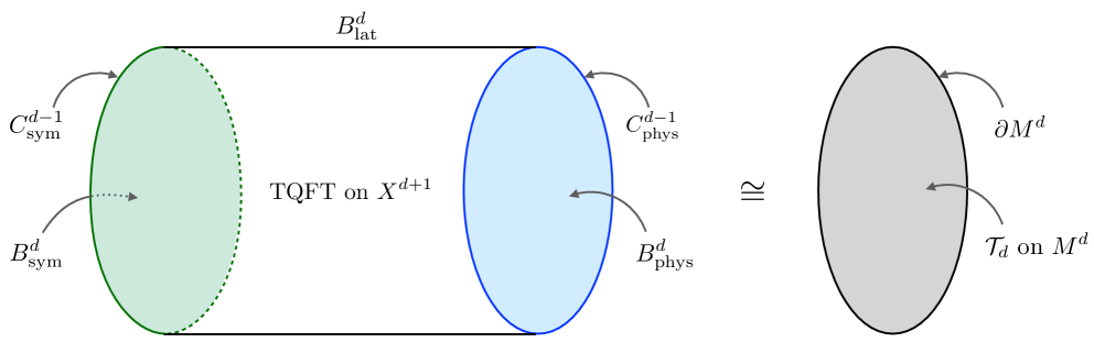
Figure 6: SymTFT realization of a theory $\mathcal{T}_{d}$ formulated on a spacetime $M^{d}$ with boundary. The bulk TQFT is formulated on $X^{d+1}=M^{d}\times[z_{0},z_{1}]$. The symmetry boundary $B^{d}_{\rm sym}=M^{d}\times\{z_{0}\}$ and the lateral boundary $B^{d}_{\rm lat}=\partial M^{d}\times[z_{0},z_{1}]$ support topological boundary conditions. They are joined along the topological interface $C^{d-1}_{\rm sym}=\partial M^{d}\times\{z_{0}\}$. The physical boundary $B^{d}_{\rm phys}=M^{d}\times\{z_{1}\}$ supports a non-topological boundary condition in general. It is joined to $B^{d}_{\rm lat}$ along the interface $C^{d-1}_{\rm phys}=\partial M^{d}\times\{z_{1}\}$, which is also non-topological in general.

The SymTFT isomorphism is well defined only if the bulk of the SymTFT is completely topological. This implies that also the boundary conditions along $B^{d}_{\text{lat}}$ must be topological. Therefore we expect that $B^{d}_{\text{sym}}$ and $B^{d}_{\text{lat}}$ are each labeled by a choice of gapped boundary conditions for the bulk SymTFT, such that $B^{d}_{\text{sym}}$ encodes the symmetry of the theory, while the choice of $B^{d}_{\text{lat}}$ dictates which part of the symmetry is left unbroken. There are now two corners, of which only one is fully topological, namely $C^{d-1}_{\text{sym}}$. The latter is a topological interface of codimension two that intertwines the symmetry boundary condition with the unbroken part of the symmetry dictated by $B^{d}_{\text{lat}}$. This is the analogue of the choice of the module $\mathcal{M}$ for $\mathcal{C}$. The latter is encoded by the corner $C^{d-1}_{\text{sym}}$. The resulting algebra $\mathcal{C}^{*}_{\mathcal{M}}$ arises along $\mathcal{B}^{d}_{\text{lat}}$. On the other side of the SymTFT interval we have $C^{d-1}_{\text{phys}}$ which is a non-topological interface between $B^{d}_{\text{lat}}$ and the physical boundary. This corner connecting the physical boundary to $\mathcal{B}^{d}_{\text{lat}}$ is then responsible for the explicit action of the symmetry on boundary conditions, encoding the spontaneous breaking on the physical theory from the bulk SymTFT description.

Let us remark that the SymTFT setup with boundaries and corners described above and depicted in Figure 6 can be used to study a physical theory $\mathcal{T}_{d}$ with a boundary that can be at infinity, or at a finite distance. The difference between these two cases is captured by the metric on the physical boundary $B^{d}_{\rm phys}$ and physical corner $C^{d-1}_{\rm phys}$. In contrast, the topological elements of the SymTFT construction – namely the bulk, $B^{d}_{\rm lat}$, $B^{d}_{\rm sym}$, and $C^{d-1}_{\rm sym}$ – do not discriminate between boundaries at infinity or at a finite distance. Our main objective in this work is to study spontaneous symmetry breaking. Therefore, we consider setups in which the metric on $B^{d}_{\rm phys}$ is such that the boundary is at infinity, which allows us to probe the long-distance infrared physics of the model, and hence the SSB.

The above is meant to give a schematic description, let us make it concrete with some examples in detail.

4.2 The case of an Abelian $p$-form symmetry

For ease of exposition, here we focus on the case of a (non-anomalous) $U(1)$ $p$-form symmetry in $d$ dimensions. We discuss the non-Abelian case for $p=0$ in Section LABEL:sec_corners_nonAb below.

4.2.1 Selected topological boundary conditions

The bulk TQFT on $X^{d+1}$ is the BF theory

$$S_{\rm bulk}=\frac{1}{2\pi}\int_{X^{d+1}}B_{d-p-1}\wedge dA_{p+1}\ ,$$ (288)

where $A_{p+1}$ is a $U(1)$ gauge field and $B_{d-p-1}$ is an $\mathbb{R}$ gauge field. Our focus is on the following topological operators of the bulk TQFT,

$$\mathbf{W}^{(n)}_{p+1}=\exp in\int_{\Sigma^{p+1}}A_{p+1}\ ,\qquad\mathbf{Q}^{(\alpha)}_{d-p-1}=\exp i\alpha\int_{\widehat{\Sigma}^{d-p-1}}B_{d-p-1}\ ,$$ (289)

where $n\in\mathbb{Z}$, $\alpha\in\mathbb{R}$, with $\alpha\sim\alpha+1$.

For concreteness, in this work we only consider two topological boundary conditions for the bulk TQFT, which we denote $\mathcal{D}_{A}$ and $\mathcal{D}_{B}$ — we refrain from attempting a classification and we do not explore the option of dressing the boundary conditions and interfaces we find with additional TQFTs. We now comment on some properties of $\mathcal{D}_{A}$, $\mathcal{D}_{B}$ and on the relevant topological interfaces between them. More details can be found in Appendix LABEL:app_Dir_and_Neu.

Topological boundary condition $\mathcal{D}_{A}$.

This is described by the action

$$S_{\rm bdy}^{\mathcal{D}_{A}}=\frac{1}{2\pi}\int_{Y^{d}}(-1)^{d-p}B_{d-p-1}\wedge(A_{p+1}-\mathcal{A}_{p+1}-d\varphi_{p})\ ,$$ (290)

where $Y^{d}=\partial X^{d+1}$, $\varphi_{p}$ is a dynamical $U(1)$ gauge field on $Y^{d}$, $\mathcal{A}_{p+1}$ is a non-dynamical $U(1)$ gauge field on $Y^{d}$, which we take to be flat,

$$d\mathcal{A}_{p+1}=0\ .$$ (291)

The sum of the bulk action and (290) is invariant under the gauge transformations

$$A_{p+1} \mapsto A_{p+1}+d\Lambda_{p}\ , B_{d-p-1} \mapsto B_{d-p-1}+d\Omega_{d-p-2}\ , \varphi_{p} \mapsto\varphi_{p}+d\sigma_{p-1}+\Lambda_{p}\ .$$ (292)

The bulk gauge parameters $\Lambda_{p}$, $\Omega_{d-p-2}$ are a $U(1)$ gauge field and a globally-defined form, respectively. The boundary gauge parameter $\sigma_{p-1}$ is a $U(1)$ gauge field. The equations of motion of the boundary action imply

$$\text{on $Y^{d}$:}\qquad A_{p+1}=d\varphi_{p}+\mathcal{A}_{p+1}\ .$$ (293)

The choice of boundary condition $\mathcal{D}_{A}$ implies that:

• An open bulk operator $\mathbf{W}_{p+1}^{(n)}$ can end perpendicularly on $Y^{d}$, on an operator of the form $e^{in\int\varphi_{p}}$.

• A closed bulk operator $\mathbf{W}_{p+1}^{(n)}$ becomes a c-number if it is projected parallel onto $Y^{d}$.

• A closed bulk operator $\mathbf{Q}_{d-p-1}^{(\alpha)}$ remains a non-trivial operator if it is projected parallel onto $Y^{d}$. We write

  $$\text{$\mathbf{Q}_{d-p-1}^{(\alpha)}$ projected onto $\mathcal{D}_{A}$:}\quad D_{d-p-1}^{(\alpha)}\ .$$ (294)

From the point of view of the bulk topological operators $\mathbf{W}_{p+1}^{(n)}$, $\mathbf{Q}_{d-p-1}^{(\alpha)}$, the topological boundary condition $\mathcal{D}_{A}$ is effectively the same as a Dirichlet boundary condition for $A_{p+1}$, and a free boundary condition for $B_{d-p-1}$. The boundary condition $\mathcal{D}_{A}$ differs from the usual Dirichlet boundary condition for $A_{p+1}$ because it is formulated including the mode $\varphi_{p}$ on the boundary. For our purposes, this is useful to study interfaces (see below).

Topological boundary condition $\mathcal{D}_{B}$.

This is described by the action

$$S_{\rm bdy}^{\mathcal{D}_{B}}=\frac{1}{2\pi}\int_{Y^{d}}(-1)^{d-p}(d\Phi_{d-p-2}+\mathcal{B}_{d-p-1})\wedge A_{p+1}\ ,$$ (295)

where $Y^{d}=\partial X^{d+1}$, $\Phi_{d-p-2}$ is a dynamical $\mathbb{R}$ gauge field on $Y^{d}$, $\mathcal{B}_{d-p-1}$ is a non-dynamical form on $Y^{d}$, which we take to be closed,

$$d\mathcal{B}_{d-p-1}=0\ .$$ (296)

The sum of the bulk action and (295) is invariant under the same bulk gauge transformations as in (292), together with

$$\Phi_{d-p-2}\mapsto\Phi_{d-p-2}+d\rho_{d-p-3}+\Omega_{d-p-2}\ ,$$ (297)

where boundary gauge parameter $\rho_{d-p-3}$ is a globally defined form. The equations of motion of the boundary action imply

$$\text{on $Y^{d}$:}\qquad B_{d-p-1}=d\Phi_{d-p-2}+\mathcal{B}_{d-p-1}\ .$$ (298)

The choice of boundary condition $\mathcal{D}_{B}$ implies that:

• An open bulk operator $\mathbf{Q}_{d-p-1}^{(\alpha)}$ can end perpendicularly on $Y^{d}$, on an operator of the form $e^{i\alpha\int\Phi_{d-p-2}}$.

• A closed bulk operator $\mathbf{Q}_{d-p-1}^{(\alpha)}$ becomes a c-number if it is projected parallel onto $Y^{d}$.

• A closed bulk operator $\mathbf{W}_{p+1}^{(n)}$ remains a non-trivial operator if it is projected parallel onto $Y^{d}$. We write

  $$\text{$\mathbf{W}_{p+1}^{(n)}$ projected onto $\mathcal{D}_{B}$:}\quad\widetilde{D}_{p+1}^{(n)}\ .$$ (299)

From the point of view of the bulk topological operators $\mathbf{W}_{p+1}^{(n)}$, $\mathbf{Q}_{d-p-1}^{(\alpha)}$, the topological boundary condition $\mathcal{D}_{B}$ is effectively the same as a Dirichlet boundary condition for $B_{d-p-1}$, and a free boundary condition for $A_{p+1}$. The boundary condition $\mathcal{D}_{B}$ differs from the usual Dirichlet boundary condition for $B_{d-p-1}$ because it is formulated including the mode $\Phi_{d-p-2}$ on the boundary.

$\mathcal{D}_{A}$-$\mathcal{D}_{A}$ interfaces.

Let us partition the boundary $\partial X^{d+1}$ into two regions $Y^{d}_{1}$ and $Y^{d}_{2}$, and impose $\mathcal{D}_{A}$ boundary conditions on both regions. The two regions meet at the interface $Z^{d-1}=\partial Y^{d}_{1}=-\partial Y^{d}_{2}$, with the minus denoting orientation reversal. We can construct a family of topological interfaces on $Z^{d-1}$. They are described by the action

$$S_{\rm int}^{\mathcal{D}_{A}\,\mathcal{D}_{A}}=\frac{1}{2\pi}\int_{Z^{d-1}}B_{d-p-1}\wedge(\varphi_{p}^{(2)}-\varphi_{p}^{(1)}-d\nu_{p-1}-\xi_{p})\ .$$ (300)

Each component $Y^{d}_{i}$ ($i=1,2$) comes with its dynamical fields $\varphi_{p}^{(i)}$ (with gauge parameters $\sigma_{p-1}^{(i)}$ as in (292)) and its non-dynamical $\mathcal{A}_{p+1}^{(i)}$. The quantity $\nu_{p-1}$ is a dynamical $U(1)$ gauge field localized on $Z^{d-1}$ with gauge transformation

$$\nu_{p-1}\mapsto\nu_{p-1}+du_{p-2}+\sigma^{(2)}_{p-1}-\sigma^{(1)}_{p-1}\ ,$$ (301)

where the parameter $u_{p-2}$ is a $U(1)$ gauge field on $Z^{d-1}$. The quantity $\xi_{p}$ in (300) is a non-dynamical form on $Z^{d-1}$, which we take such that

$$\text{on $Z^{d-1}$:}\qquad d\xi_{p}=\mathcal{A}^{(1)}_{p+1}-\mathcal{A}^{(2)}_{p+1}\ .$$ (302)

We regard $\xi_{p}$ as a parameter that labels various possible $\mathcal{D}_{A}$-$\mathcal{D}_{A}$ interfaces. We give more comments on its physical interpretation in Section LABEL:sec_Goldstone below, where we connect it to the degeneracy of vacua expected for a theory with SSB of a continous symmetry.

An important property of $\mathcal{D}_{A}$-$\mathcal{D}_{A}$ interfaces of the form (300) is the following. On either side of the interface we can insert an operator $D^{(\alpha)}_{d-p-1}$ (see (294) for the definition) supported on a cycle $\Sigma^{d-p-1}$. If we project $D^{(\alpha)}_{d-p-1}$ parallel to the interface, the interface absorbs it. In the process, the interface parameter $\xi_{p}$ shifts

$$\xi_{p}\rightarrow\xi^{\prime}_{p}=\xi_{p}+2\pi\alpha\delta_{p}(\Sigma^{d-p-1}\subset Z^{d-1})\ ,$$ (303)

where $\delta_{p}(\Sigma^{d-p-1}\subset Z^{d-1})$ is the Poincaré dual to $\Sigma^{d-p-1}$ in $Z^{d-1}$. We refer the reader to Appendix LABEL:app_Dir_and_Neu for more details.

$\mathcal{D}_{A}$-$\mathcal{D}_{B}$ interface.

Let us partition the boundary $\partial X^{d+1}$ into two regions $Y^{d}_{1}$ and $Y^{d}_{2}$, and impose $\mathcal{D}_{A}$ boundary conditions on $Y^{d}_{1}$ and $\mathcal{D}_{B}$ on $Y^{d}_{2}$. As above, the two regions meet at the interface $Z^{d-1}=\partial Y^{d}_{1}=-\partial Y^{d}_{2}$. This time we construct a single topological interface, described by the action

$$S_{\rm int}^{\mathcal{D}_{A}\,\mathcal{D}_{B}}=\frac{1}{2\pi}\int_{Z^{d-1}}\bigg[(-1)^{d-p}\Phi_{d-p-2}\wedge d\varphi_{p}+(-1)^{d-p}\Phi_{d-p-2}\wedge\mathcal{A}_{p+1}-\mathcal{B}_{d-p-1}\wedge\varphi_{p}\bigg]\ .$$ (304)

We notice the BF coupling between the mode $\varphi_{p}$ from the $\mathcal{D}_{A}$ side, and the mode $\Phi_{d-p-2}$ from the $\mathcal{D}_{B}$ side.

An important property of the $\mathcal{D}_{A}$-$\mathcal{D}_{B}$ interface is the following. On the $\mathcal{D}_{A}$ side of the interface, we can insert an operator $D^{(\alpha)}_{d-p-1}$. If we project it parallel to the interface, it becomes a c-number. Alternatively, we can have an open $D^{(\alpha)}_{d-p-1}$ operator inside $Y^{d}_{1}$ ending perpendicularly on the interface, on an operator of the form $e^{i\alpha\int\Phi_{d-p-2}}$.

Similarly, on $\mathcal{D}_{B}$ side of the interface, we can insert an operator $\widetilde{D}^{(n)}_{p+1}$ (see (299) for the definition). If we project it parallel to the interface, it becomes a c-number. Alternatively, we can have an open $\widetilde{D}^{(n)}_{p+1}$ operator inside $Y^{d}_{2}$ ending perpendicularly on the interface, on an operator of the form $e^{in\int\varphi_{p}}$.

4.2.2 Scenarios for unbroken and broken symmetry

In this subsection we adopt the general picture described in Section 4.1 and we describe the choices of $B^{d}_{\rm sym}$, $B^{d}_{\rm lat}$, $C^{d-1}_{\rm sym}$ that correspond to different scenarios for a $U(1)$ $p$-form symmetry. For simplicity, we focus on two the extreme scenarios in which the symmetry is either completely unbroken, or completely broken. Our proposal to describe these scenarios is encoded in the following table

$$\begin{array}[]{|l|>{\centering}p{1.2cm}| >{\centering}p{1.2cm}| >{\centering\arraybackslash}p{3.2cm}|}\hline\cr&$B^{d}_{\rm sym}$ \rule[-7.11317pt]{0.0pt}{19.91684pt}\@add@centering&$B^{d}_{\rm lat}$\@add@centering&\end{array}$$ (407)