Dual-Backend Multibeam Position Switching Targeted SETI Observations toward Nearby Active Planet-Hosting Systems with FAST

Abstract

The Five-hundred-meter Aperture Spherical Telescope (FAST), the world’s largest single-dish radio telescope, lists the search for extraterrestrial intelligence (SETI) as one of its key scientific objectives. In this work, we present a targeted SETI observation for 7 nearby active stars utilizing the FAST L-band multibeam receiver, employing a observational strategy that combines position switching with multibeam tracking to balance on-source integration time with the accuracy of the beam response. Using both pulsar and SETI backends, we perform a comprehensive search for narrowband drifting signals with Doppler drift rates within $\pm 4\ \mathrm{Hz\ s^{-1}}$ and channel-width periodic signal with periods between 0.12 and 100 s and duty cycles between 10% and 50%. No credible radio technosignatures were detected from any of the target systems. Based on this null result, we place constraints on the presence of transmitters at a 95% confidence level, ruling out narrowband transmitters with with EIRP above $3.98\times 10^{8}\,\mathrm{W}$ and periodic transmitter with EIRP above $1.80\times 10^{10}\,\mathrm{W}$,respectively, within the observation band.

1 Introduction

The Search for Extraterrestrial Intelligence (SETI) endeavors to detect evidence of technologically advanced civilizations beyond Earth by looking for technosignatures, especially in radio frequency. To maximize the chances of discovery, many SETI programs focus on targeted observations of selected targets. In practice, this means pointing sensitive radio telescopes at certain celestial locations where the potential for detecting an artificial signal can be enhanced, such as planet-hosting stars (Siemion et al., 2013; Tingay et al., 2016; Harp et al., 2016; Enriquez et al., 2017a; Pinchuk et al., 2019; Price et al., 2020; Sheikh et al., 2020; Traas et al., 2021; Smith et al., 2021; Margot et al., 2021; Gajjar et al., 2022; Tao et al., 2022, 2023; Luan et al., 2025), Galactic center (Tremblay & Tingay, 2020; Gajjar et al., 2021; Brzycki et al., 2024), and nearby galaxies (Gray & Mooley, 2017; Choza et al., 2024). Despite decades of targeted SETI observations, no confirmed technosignature has been found, underscoring the need for continued searches with ever-improving instruments and strategies.

The detection for thousands of exoplanets over the past three decades reflects a transformative period in astronomy, revealing that planetary systems are ubiquitous around most stars in the Milky Way (MW). Cassan et al. (2012) suggested that, in our Galaxy, at least one planet per star averagly, and Petigura et al. (2013) found that approximately 22% of Sun-like stars contain an Earth-sized planet within their temperate habitable zones (HZ). Many of the known exoplanets in or near HZ orbit M dwarf, which are smaller and cooler than the Sun, and consist about 75% of all stars in the Galaxy. Notably, such stars often exhibit stronger magnetic fields (Johns-Krull & Valenti, 1996; Reiners et al., 2009; Shulyak et al., 2017; Kochukhov, 2021) and higher activity levels (Kiraga & Stepien, 2007). Particularly, they can powerful flares and bursts from X-rays to radio waves (Kowalski, 2024), hence affect the planetary habitability. Strong and frequent flare stellar activities and coronal mass ejections (CMEs) can erode planetary atmospheres, making the planet uninhabitable (Khodachenko et al., 2007; Kay et al., 2016; Vida et al., 2017; Garcia-Sage et al., 2017). On the other hand, it is still debated that tidally locked planets might still retain habitable for some certain suitable conditions (Tarter et al., 2007; Yang et al., 2013; Wandel, 2023). Thus, M dwarf star systems remain central to exoplanet habitability studies and SETI target lists. Beyond M dwarfs, other types of star can also provide habitable environments around their orbit. Closely adjacent to the Sun on the stellar spectrum are K-type and F-type stars, both recognized as potentially promising hosts for life-bearing worlds. K dwarfs, comprising about 15% of main-sequence stars, are also known as “Goldilock” stars since they can exhibit moderate stellar activity, as well as relatively stable and gentle radiation environments, which enhance their suitability for hosting planets with stable atmospheres and climates (Cockell, 1999; Cuntz & Guinan, 2016). F-type stars, though comparatively rare, possess broader and farther HZ allowing Earth-like planets to avoid tidal locking (Sato et al., 2017), while their stronger ultraviolet radiation could be harmful to DNA (Sato et al., 2014). Although F-type stars are paid less habitability consideration, the above circumstellar environments features are still potential for life existstence (Patel et al., 2024).

The unprecedented sensitivity of FAST (Nan, 2006; Nan et al., 2011; Li & Pan, 2016; Jiang et al., 2020) provides a valuable opportunity to expand SETI research (Li et al., 2020; Chen et al., 2021). Previous SETI efforts with FAST have primarily focused on looking for continuous narrow-band signals using the 19-beam L-band receiver in a single-pointing tracking mode. A given star system is observed by one of the beams while the others serve as reference beams and the candidate should only appear in the on-target beam but not in the reference beams (Tao et al., 2022, 2023; Luan et al., 2023, 2025; Huang et al., 2023), which can reject a considerable part of radio frequency interference (RFI). Neverthless, the gains and leakages of different beams can vary remarkably, which may lead ambiguity in distinguish candidate and RFI. These earlier FAST observations employed single dedicated SETI backend for narrowband signal expected to be Doppler-drifted (Sheikh et al., 2019; Li et al., 2022; Li et al., 2023). Recently, It has been suggested that broadband signal might be preferred than narrowband signal duw to the terrestrial economics of beacon transmitter (Benford et al., 2010a, b), the employing of frequency-shift keying (Fridman, 2011) and the consideration of robustness to RFI (Messerschmitt & Morrison, 2012; Messerschmitt, 2012). In observations, Gajjar et al. (2021, 2022) have carried out boardband signal search in SETI observation by identifying artificial dispersion, and Suresh et al. (2023) have searched the periodic technosignatures by the repeating period of the signal. Overall, the fundamental principle in SETI is to identify signals that are distinguishable from natural astrophysical emission, not merely limited to narrowband features.

In this paper, we propose a combination of multibeam method and position switching observations. The central beam serves as on-target beam and the edge beams serve as reference beams in the on-source observation. When switching telescope direction, one of the edge beam point at the target source to serve as on-target beam, while the other beams serve as reference beam. The instrumental factors can be calibrated by on-off switching, and the RFI rejection efficiency can be enhanced both by on-off and multibeam. Furthermore, We also utilize pulsar (psr) backend and SETI backend to record high temporal resolution data and high-frequency resolution data simultaneously during SETI observations. The dual-backend approach allows us to conduct two complementary searches on the same observation targets. The high-frequency resolution data is for the conventional narrowband, continuous-wave drifting signals, while the high temporal resolution data is for channel-width periodic signal search. In section 2, we discuss the observation targets and strategy in this work. The data process pipeline and princeple are introduced in section 3, and the corresponding results are presented in section 4. Section 5 is the implication of our results and section 6 lists the conclusion of this work.

2 Observations

2.1 Targets

We prioritize 7 stellar systems for our SETI survey based on their astrobiological potential, observability, as well as relative proximities to Earth. Targets are chosen for their high astrobiological potential to increase the likelihood of life. Nearby stellar systems are prioritized to enhance signal detectability. We also confirme that all targets are practically observable, with celestial positions falling within the accessible sky of our telescope. A comprehensive summary of these targets is provided in Table 1, with their sky distribution visualized in Figure 1. We also observe 3C286, 3C48 and 3C147 as flux calibrators.

Table 1: Information of the Observation Targets in This Work.

Source Name	R.A. (J2000.0)(1)	Decl. (J2000.0)(1)	Distance (pc)(1)	Spectral Type	Luminosity ($L_{\odot}$)	Temperature (K)	Exoplanet Candidate
Barnard’s Star	17:57:48.50	+04:41:36.11	1.83	M4V(2)	0.00340(9)	3195(13)	Barnard’s Star b, c, d, e(15)
Ross 128	11:47:44.40	+00:48:16.40	3.37	M4V(3)	0.00366(9)	3189(9)	Ross 128 b(16)
Gliese 581	15:19:26.83	-07:43:20.19	6.30	M3V(4)	0.012365(10)	3500(10)	Gliese 581 b, c , d, e, f, g(17)
Upsilon Andromedae A	01:36:47.84	+41:24:19.65	13.48	F8V(5)	3.1(11)	6614(11)	Upsilon Andromedae A b, c, d(18)
55 Cancri A	08:52:35.81	+28:19:50.96	12.59	K0IV-V(6)	0.617(12)	5172(14)	55 Cancri A b, c, d, e, f(19)
Lalande 21185	11:03:20.19	+35:58:11.58	2.55	M2V(7)	0.02194(9)	3547(9)	Lalande 21185 b, c, d(20)
Wolf 359	10:56:28.92	+07:00:53.00	2.41	M6V(8)	0.00106(9)	2749(9)	Wolf 359 b(21)

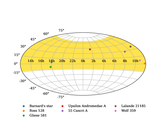
Figure 1: Observation targets in equatorial coordinates. The observable sky coverage of FAST is filled by yellow color.

2.1.1 Planetary Habitability

Planetary habitability is one of the key factors prioritizing target selection for SETI observations (Tarter, 2001, 2004; Turnbull & Tarter, 2003). Stars with planets located within HZ are considered prime candidates which are possible to maintain liquid water on planetary surfaces, increasing the likelihood of life and, consequently, potential technosignatures. We also estimate the planetary habitabilities around these stars using the stellar flux HZ model in Kopparapu et al. (2013) and the “Habitable Zone for Complex Life (HZCL)” model in Schwieterman et al. (2019), in which the stellar effective temperatures, stellar luminosity, $\text{H}{\vphantom{\text{X}}}_{\smash[t]{\text{2}}}\text{O}$ and $\text{CO}{\vphantom{\text{X}}}_{\smash[t]{\text{2}}}$ absorption coefficients, as well as the planetary atmospheric $\text{CO}{\vphantom{\text{X}}}_{\smash[t]{\text{2}}}$ pressure are taken in to consideration. Figure 2 illustrates the boundaries of the HZ.

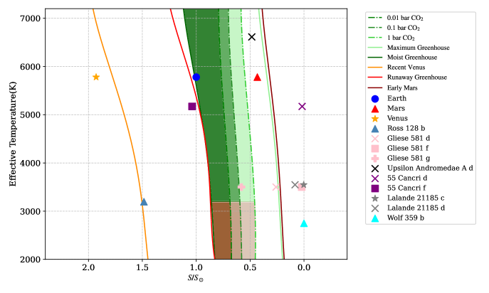
Figure 2: Various HZ boundaries for stars with different effective temperatures. The five solid lines are the HZ boundaries determined by stellar flux HZ model of Kopparapu et al. (2013), and the green and brown shaded regions are the HZCL model of Schwieterman et al. (2019) assuming limiting $\text{CO}{\vphantom{\text{X}}}_{\smash[t]{\text{2}}}$ concentrations of 0.01 bar (dark green), 0.1 bar (lighter green), and 1 bar (lightest green). The brown contours denote regions around low-temperature stars where photochemical effects could allow CO concentrations to exceed short-term human safety thresholds ($>100$ ppm) at the moist greenhouse boundary, under an assumed surface flux of $3\times 10^{11}$ molecules cm^-2 s^-1. The planetary parameters are from Basant et al. (2025) for Barnard’s star, Liebing et al. (2024) for Ross 128, von Stauffenberg et al. (2024); Vogt et al. (2010) for Gliese 581, Ligi et al. (2012) for Upsilon Andromedae A, Dawson & Fabrycky (2010); Winn et al. (2011); Bourrier et al. (2018) for 55 Cancri A, Hurt et al. (2022) for Lalande 21185, and Tuomi et al. (2019); Bowens-Rubin et al. (2023) for Wolf 359.

We can see that Upsilon Andromedae A d and Gliese 581 d are near the edge of maximum greenhouse, and Gliese 581 g, if it exists, falls in the HZCL. The estimation of habitabilities of exoplanets would be one of the crucial factors in our target selection for targeted SETI observations.

2.1.2 Stellar Activities

Stellar magnetic activities, especially stellar flare activities, can significantly impact the radiation environment encountered by planets, making it an essential role in promoting or destroying planetary habitabilities. Generally, intense stellar flares and radiation bursts are viewed negatively, as they may severely erode planetary atmospheres or expose surfaces to sterilizing radiation (Airapetian et al., 2017; Garcia-Sage et al., 2017), consequently threaten the habitability for complex life-forms. It is proposed that, on the other hands, moderate, or even intense, energetic eruptive stellar activity might drive the planetary atmosphere dynamics via interactive photochemistry, thereby affect the climate and atmospheric evolution of the planet (Konings et al., 2022; Berger et al., 2024; Chen et al., 2025). Moerover, the synthesis of some vital biochemical products for complex life, such as Vitamin D (Spinelli et al., 2023), amino acids (Sarker et al., 2013), and ribonucleic acid (Powner et al., 2009; Ranjan & Sasselov, 2016; Rimmer et al., 2018), can be triggered under the condition of ultraviolet (UV) light from stellar radiation and flare.

Most of flare stars are M dwarfs (Pettersen & Hawley, 1989; Giampapa, 2000), and many flare activities are detected from the selected observation targets, including Barnard’s star (Paulson et al., 2006; France et al., 2020), Ross 128 (Lee & Hoxie, 1972), Lalande 21185 (Schmitt et al., 1995; Pye et al., 2015) and Wolf 359 (Gershberg & Shakhovskaia, 1983; Robinson et al., 1995; Schmitt et al., 1995; Liefke et al., 2007), while Gliese 581 exhibits relatively low stellar activity, reducing the threat to atmospheric retention and making it comparatively more favorable for sustaining habitable environments. K-type star 55 Cancri A and F-type star also show stable, moderate activities.

2.1.3 SETI Search for the Targets

Some of the observation targets are also listed in some SETI related project. A digital radio signal named “A Message from Earth” has been sent towards Gliese 581, and a message call “Cosmic call 2” has been sent towords 55 Cancri, respectively, by the Yevpatoria RT-70 radio telescope. Gliese 581 is targeted by the first Very Long Baseline Interferometric (VLBI) SETI experiment, while no candidate was found (Rampadarath et al., 2012). A anomalous unpolarized radio emission was detected during the observation of Ross 128 , which is confirmed to be RFI by the follow-up observation (Enriquez et al., 2017b, a). Previous FAST SETI observations also attempt to search radio technosignature from Barnard’s star (Tao et al., 2023) and Wolf 359 (Luan et al., 2025).

2.2 Strategy

Currently, there are 10 categories of observation mode and 3 digital backend for FAST, working at the frequency range of 1.05 GHz-1.45 GHz with full-polarization measurements from two linear feeds. Previously, drifting scan (Zhang et al., 2020), tracking (Tao et al., 2022, 2023; Luan et al., 2023, 2025), and multibeamOTF (Huang et al., 2023) modes are employed in the FAST SETI observation. To make full use of the layout of the 19-beam receiver and the digital backends of FAST, as well as to improve the RFI rejection process by instrumental calibration, we employ position switching observation mode and record data with both psr backend and SETI backend. For flux and polarization calibration, we also inject linearly polarized noise diode signals with temperature of $\sim 12.5\,\mathrm{K}$ for $\sim 5\,\mathrm{s}$ at the beginning of the first and last ON and OFF observations, respectively.

2.2.1 Multibeam Position Switching Mode

The on-off strategy, or generally, position switching, is a standard observation mode for targeted SETI and spectral line studies, which implements repetitive paired cycles of telescope movements between on-source and adjacent off-source positions at matched airmass. For SETI applications, artificial technosignatures are expected to manifest exclusively in on-source observations while remaining statistically absent in off-source reference data, providing critical discrimination against terrestrial RFI and instrumental artifacts (Enriquez et al., 2017a). For large single-dish radio telescopes, multibeam observations are often used in large sky serveys for high efficiency (Staveley-Smith et al., 1996; Cordes et al., 2006; Li et al., 2018).

Multibeam strategy has also been implemented in targeted SETI observations using FAST’s 19-beam receiver, significantly enhancing temporal efficiency and RFI mitigation capabilities (Tao et al., 2022; Luan et al., 2023). Spatial beam diversity provides multiple concurrent reference positions, enabling advanced RFI discrimination through coverage pattern analysis. Nevertheless, beam variations in gain, aperture efficiency, system temperature, and polarization leakage can compromise RFI rejection validity without rigorous per-beam calibration.

The position switching observation is also a fundamental calibration technique essential for radio astronomy. By pointing the telescope at the target (on) and then at a nearby empty patch of sky (off), the background noise the atmosphere and the instrument itself can be measured and subtracted, which enable us to calculate the system’s true sensitivity. The observation modes we use in this work are OnOff mode and PhaseReferencing mode, the observation details of the sources are listed in Table 2. The basic position switching for FAST is OnOff mode, where the on-source point and off-source point are observed with equal time, while PhaseReferencing, one of the OnOff mode extension, enables us to set the observation time and the positions for the on-source point and off-source point separately.

Table 2: Observation Details of the Targets in This Work.

Target	Observation Date	Observation Mode	OFF R.A. (J2000.0)	OFF Decl. (J2000.0)	Off-source Beam
3C286	2024-11-15	OnOff	13:31:08.28	+30:00:32.9	–
Barnard’s Star	2024-11-15	OnOff	17:57:47.67	+04:14:16.7	–
Ross 128	2024-11-15	OnOff	11:47:45.02	+00:17:57.4	–
3C48	2025-07-09	PhaseReferencing	01:38:08.58	+33:19:32.7	12
3C147	2025-07-09	PhaseReferencing	05:43:11.56	+50:01:04.8	12
3C286	2025-07-09	PhaseReferencing	13:32:01.68	+30:30:34.8	14
Gliese 581	2025-07-09	PhaseReferencing	15:20:13.25	$-$07:43:18.4	14
Upsilon Andromedae A	2025-07-09	PhaseReferencing	01:37:49.17	+41:24:21.5	14
55 Cancri A	2025-07-09	PhaseReferencing	08:53:28.07	+28:19:52.8	14
Lalande 21185	2025-07-09	PhaseReferencing	11:04:17.03	+35:58:13.4	14
Wolf 359	2025-07-09	PhaseReferencing	10:56:51.93	+07:10:50.6	12

References. — (1) Gaia Collaboration et al. (2023); (2) Gizis (1997); (3) Gautier et al. (2004); (4) Bonfils et al. (2005); (5) Abt (2009); (6) Gray et al. (2003); (7) Keenan & McNeil (1989); (8) Henry et al. (1994); (9) Pineda et al. (2021); (10) von Stauffenberg et al. (2024); (11) Baines et al. (2021); (12) Soubiran et al. (2024); (13) González Hernández et al. (2024); (14) Bourrier et al. (2018); (15) The four planets orbiting Barnard’s star are proposed by González Hernández et al. (2024) and comfirmed by Basant et al. (2025); (16) Ross 128 b is discovered by Bonfils et al. (2018), and Liebing et al. (2024) comfirms that this planet retains status as hosting lonely; (17) Currently, the existstence of Gliese 581 b, c and e have been comfirmed (Robertson et al., 2014; Trifonov et al., 2018; von Stauffenberg et al., 2024), the existstence of Gliese 581 f and g are refuted (Robertson et al., 2014, 2013), and the existstence of Gliese 581 d still remains doubtful and under vigorous debate as it is thought to be a false positive result from stellar activity (Robertson et al., 2014; Suárez Mascareño et al., 2015; Hatzes, 2016; Trifonov et al., 2018; Dodson-Robinson et al., 2022; von Stauffenberg et al., 2024), whlie some studies still support its existstence (Vogt et al., 2012; Hatzes, 2016; Cuntz et al., 2024); (18) Upsilon Andromedae A has once been thought to host four planets (Barnes & Greenberg, 2008; Curiel et al., 2011), but the existstence of Upsilon Andromedae e is still suggested to be instrumental artifact (McArthur et al., 2014; Deitrick et al., 2015); (19) The 55 Cancri A planetary system is confirmed by Butler et al. (1997); Marcy et al. (2002); McArthur et al. (2004); Fischer et al. (2008), and it is suggested that a hypothetical planet g exist in the gap between planets f and d Raymond et al. (2008); (20) Lalande 21185 b is comfirmed by Stock et al. (2020) and Lalande 21185 c is comfirmed by Rosenthal et al. (2021), planet d is suspected to orbit between planet b and c Hurt et al. (2022); (21) Wolf 359 b is reported by Tuomi et al. (2019) while its existence is unable to be either confirmed or refuted (Bowens-Rubin et al., 2023).

Our observation strategy employs a on-off cycle with 3 repetitions for each target. In the On-Off observations, we set the observation time for each On/Off as 6 minutes. The off-source position is defined by a $0.5^{\circ}$ offset in declination from the on-source target. The angular separation is significantly larger than the Full-Width Half-Maximum (FWHM) beamwidth of FAST at 1.4 GHz (approximately $2.9^{\prime}$), ensuring that the target source is well outside the primary beam of FAST during off-source measurements. Such configuration guarantees that any signals detected in the off-source across multiple beams can be identified as RFI. While the PhaseReferencing observations consist of 6-minute on-source time and 30-second off-source time. By carefully setting the off-source coordinates, the telescope’s pointing is optimized such that when the central beam is positioned on the off-source location, a designated edge beam simultaneously points at the on-source target (See Figure 3 (b)).

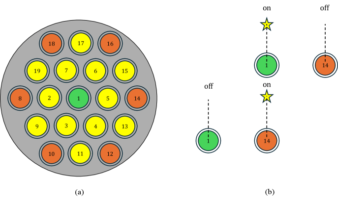
Figure 3: A simple diagram for (a) the multibeam layout of FAST and (b) an example of multibeam position switching method. In the on-source observations, the central beam 1 points at the target, serving as “On”. In the off-source, one of the edge beam 14 switchs to the location pointing at the target, serving as “On”, while beam 1 serves as “Off”.

This interleaved approach allows us to conduct a necessary off-source observation for one beam while simultaneously performing an on-source observation for another, effectively increasing the on-target integration time within a given observing window.

2.2.2 FAST Digital Backend

There are three kinds of backends for FAST : psr, spectral (spec) and SETI, which can be in different combinations with single or multiple backend configuration. Since the SETI and spec backends use the same computing resources, the SETI and spec data cannot be recorded simultaneously. For sake of high temporal resolution and high-frequency resolution, we select SETI backend with $\sim 10\,\mathrm{s}$ sampling time and 65536k channels, and psr backend with $49.152\,\mathrm{\mu s}$ sampling time and 4096 channels. The details of FAST multibeam digital backend are described in Zhang et al. (2020); Li et al. (2020). After the observations, we can obtain psrfits files with psr backend and sdfits files with SETI backend. All these FITS files are merged in order for each beam, and converted into Filterbank files containing two dimensional time-frequency power spectra of the four polarization channels: XX, YY, XY and YX, which are derived from self-correlation and cross correlation of the data in two orthogonal linear polarization directions X and Y. The psrfits files are converted into Filterbank files by digifil in DSPSR (van Straten & Bailes, 2011), and the sdfits files are converted into Filterbank files by filterbank package in PRESTO (Ransom, 2011). All these Filterbank files are accessible to the Blimpy package (Price et al., 2019).

3 Data Process and Analysis

Given that the duration of noise diode signals is shorter than the backend sampling time in SETI observations, we explicitly subtract these signals from PSRFITS data based on their precise injection timestamps. The noise diode injections correct amplitude mismatches between the two linear polarization feeds. Digitized outputs are converted to antenna temperature $T_{a}$ using the noise diode calibration report, with flux density scaling achieved through observations of calibrators. We flag RFI channels by firstly identifying and masking significant outliers in the time-averaged spectrum, defined as channels with intensities deviating from the global median and median absolute deviation (MAD). Subsequently, a smooth spectral baseline is estimated by applying a median filter to the remaining unflagged channels. This baseline is used to identify weaker RFI by flagging any channels where the residual spectrum exceeds the fluctuation threshold (See Appendix A for details).

Narrowband drifting signal search can be done by TurboSETI, a python-cython package to search for narrowband signals via Taylor-tree de-doppler algorithm (Taylor, 1974; Siemion et al., 2013; Enriquez et al., 2017a; Enriquez & Price, 2019). Narrowband continuous signals of extraterrestrial origin should exhibit Doppler frequency drift at a rate $\mathrm{d}\nu/\mathrm{d}t$ due to the relative motion in the line of sight (Li et al., 2022). Over short observational timescales, this drift rate is effectively constant, producing a linear frequency variation. TurboSETI amis to search such drifting signal above the signal-to-noise ratio (SNR) threshold within a given maximum drift rate (MDR). Following many previous targeted SETI observations, we set the SNR threshold as 10 and the MDR as 4 Hz/s.

We employ the blipss pipeline (Suresh et al., 2023) to search for periodic pulsed signals from the psr backend data, utilizing a Fast Folding Algorithm (FFA) for channel-wide periodicity detection. The parameters used in the search are listed in Table 3.

Table 3: Parameter values used in blipss search in this work.

Parameter	Value
Running median width, $W_{\mathrm{med}}$	12 s
Range of trial periods $P$	0.12-100 s
Pulse duty cycle resolution	10%
Range of trial duty cycles $\delta$	10%-50%
S/N threshold for ON pointings	8
S/N threshold for OFF pointings	6

While most parameters adopt the default configurations from Suresh et al. (2023), the minimum trial period is explicitly set to 0.12 s, which still satisfies the fundamental constrain $P_{\min}\geqslant N_{\mathrm{bins}}t_{\mathrm{samp}}$ with $N_{\mathrm{bins}}=10$ being the minimum bin number across a folding period. Valid candidates must exhibit statistically significant folded pulse profiles detected exclusively in on-source observations.

To avoid ambiguity and maintain consistency, we define signals detected above signal-to-noise ratio threshold as hit. A set of hits present in “On” observations with relatively noticeable continuities in time or frequency are grouped into an event. Event that contain no hits in all “Off” observations are defined as candidate. For narrowband drifting signal, the definations of event $\epsilon_{\mathrm{NB}}$ and candidate $\mathcal{C}_{\mathrm{NB}}$ can be formulated by Equation (1) and (2) via hits $h$ (Traas et al., 2021):

$$\epsilon_{\mathrm{NB}}=\{h\in\mathrm{On_{k}}:\nu_{0}-\dot{\nu}_{0}\tau_{\mathrm{obs}}\leqslant\nu_{h}\leqslant\nu_{0}+\dot{\nu}_{0}\tau_{\mathrm{obs}}\},$$ (1)

$$\mathcal{C}_{\mathrm{NB}}=\{h\in\mathrm{On_{k}}:h\notin\mathrm{Off}\cap\nu_{0}-\dot{\nu}_{0}\tau_{\mathrm{obs}}\leqslant\nu_{h}\leqslant\nu_{0}+\dot{\nu}_{0}\tau_{\mathrm{obs}}\},$$ (2)

where $\nu_{h}$ is the frequency of a hit in the kth “On” observation, $\nu_{0}$ and $\dot{\nu}_{0}$ are the central frequency and corresponding drift, respectively. For periodic signal, event $\epsilon_{\mathrm{P}}$ and candidate $\mathcal{C}_{\mathrm{P}}$ can be defined by

$$\epsilon_{\mathrm{P}}=\{h\in\mathrm{On_{k}}:P_{\min}\leqslant P_{h}\leqslant P_{\max}\},$$ (3)

$$\mathcal{C}_{\mathrm{P}}=\{h\in\mathrm{On_{k}}:h\notin\mathrm{Off}\cap P_{\min}\leqslant P_{h}\leqslant P_{\max}\},$$ (4)

where $P_{h}$ refers to the period of the hits’ appearance in the frequency channel.

4 Results

4.1 Narrowband Signal Search

In the narrowband drifting signal search, we found 492921 hits in XX polarization channel and 470851 hits in YY polarization channel after running turboSETI. Among these hits, 9323 events in XX and 9407 events in YY are detected in the on-source observations. The distributions of frequency, drift rate, and signal-to-noise ratio are illustrated in Figure 4 and 5, and some known RFI sources within the observation frequency ranges (Wang et al., 2021) are also shown in the plots.

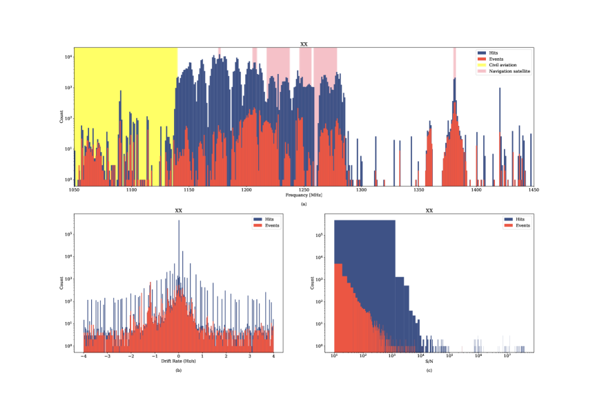
Figure 4: Histograms of the distributions of frequency, drift rate and signal-to-noise ratio in XX channel. The frequency bands of some known interference sources are displayed on the frequency panel.

Figure 5: Similar histograms of the distributions of frequency, drift rate and signal-to-noise ratio in YY channel.

A considerable amount of hits fall in the frequency ranges of civil aviations (1.27% for XX and 1.71% for YY, respectively) and navigation satellites (24.11% for XX and 24.84% for YY, respectively), implying that about 30% RFIs may come from these knows sources. 195 events in XX and 217 events in YY fall near the frequencies of the clock oscillators used by the Roach 2 FPGA board, wihch can be calculated by the linear combinations ofthe nominal frequencies 33.3333 and 125.00 MHz. We also reexamine the selected events by visual inspection of the time-frequency spectra. Almost all of the selected events are false positives mentioned in Tao et al. (2022), which can be directly excluded. We also find some events that only occupy several time-frequency pixels, instead of spanning the full on-source time. Figure 6 (a) is one of the examples of such event. These events can be excluded by examining other events with similar feature that also appear within frequency ranges of known RFI sources (See the b panel of Figure 6).

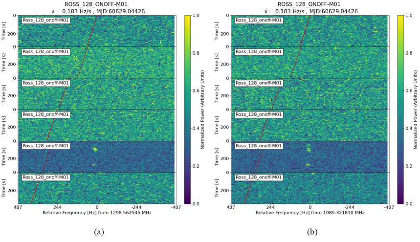
Figure 6: Examples of RFIs that only occupy several time-frequency pixels. Panel (a) is an event that appears in 1298.562058 MHz, which is not the categorized as RFI frequency ranges. Panel (b) is an event that appears in 085.321323 MHz, which fall in the frequency of civil aviations.

4.2 Periodic Pulsed Signal Search

For the OnOff observations in 2024 November 15, we divide observation data into 3 On and Off 6-minute series respectively and carry out FFA search in single beam. For the PhaseReferencing observations in 2025 July 9, the central and reference beams alternate roles as asymmetric On and Off observation, we can conduct FFA search for the 6-minute and 30-second series composed by the two beams. The results of the FFA search are listed in Table 4, including 1830177 $F_{1}$ candidates and 585178 $F_{2}$ candidates in total. The candidate differences in number may be caused by the seasonal RFI environment at FAST, and the diverse gain responses in different beams.

Table 4: Candidate Statistics for Target Sources

Source	$F_{1}$	$F_{2}$	$N_{\mathrm{event}}$
Barnard’s Star	6283	0	55135
Ross128	7603	0	59777
55 Cancri A	898530	276513	5155016
Gliese 581	351232	130461	5211503
Lalande 21185	218800	81791	987255
Upsilon uAndromedae A	206928	69961	1329432
Wolf 359	192133	72336	1186105
Total	1881509	631062	13984223

Figure 7 exhibits the statistical distribution of candidates in $\nu-P$ and $\nu-\mathrm{S/N}$ diagrams. The statistics reveals that most of the candidates are predominantly populated by RFI, wihch is evidenced by the nearly identical statistical distributions of $F_{1}$ and $F_{2}$ candidates across both period and signal-to-noise ratio, strongly suggesting a common origin. Crucially, both populations densely populate almost the whole frequency-period parameter space, and cluster within narrow, persistent radio frequency channels.

Figure 7: Statistical distribution of $F_{1}$ (blue) and $F_{2}$ (red) in the search.Top left panel: histogram of the candidate periods. Top right panel: histogram of the signal-to-noise ratio of the candidates. Bottom left panel: scatter of candidates in $\nu-P$ plane. Bottom right panel: scatter of candidates in $\nu-\mathrm{S/N}$ plane.

To substantially reduce the candidates, we entirely discard candidates from frequency channels with severe persistent RFI within 1140 MHz to 1290 MHz. Specifically, for the remaining candidates, we perform a comparison with candidates detected during "Off" observations. A candidate should be excluded as RFI if its period and signal-to-noise ratio (S/N) are similar to those of a events found in the same frequency channel during an “Off” scan, assuming they share a common terrestrial origin. Figure 8 shows the statistical distribution of the candidate population after this comprehensive filtering process.

Figure 8: Statistical distribution of $F_{1}$ (pink) and $F_{2}$ (yellow) in the search silimar to Figure 7 but after filtering.

A subset of remaining candidates still clustered at specific periods after applying the filtering, wihch means broadband pulses may appear in the observation. We generated phase-resolved spectra for each source by folding at the most probable period identified from the candidates’ probability density of density. An example of the period probability density distribution for the remaining candidates, derived from the Lalande 21185 observation, is presented in the left panel of Figure 9. Visual inspection of these spectra yields no evidence of periodic signal or dispersed pulse in the corresponding frequency channel. Consequently, we attribute these remaining candidates to stochastic fluctuations in the noise. The right panel in Figure 9 is the example for the phase-resolved spectrum of Lalande 21185. Except shade in the frequency channels that contaminated by RFI severely, no obvious pulse or periodicity is found in it.

Figure 9: Left panel: The probability density profile for the periods of the remaining candidates in the observation of Lalande 21185. The peak of the probability density is $P=7.45293$ s. Right panel: The phase-resolved spectrum of the observation of Lalande 21185 for the most probable period identified from the probability density in the left panel.

5 Discussion

5.1 Sensitivity

The sensitivity of a radio observation can be determined by system equivalent flux density (Wilson et al., 2013; Thompson et al., 2017)

$$\mathrm{SEFD}=\frac{2k_{\mathrm{B}}T_{\mathrm{sys}}}{A_{\mathrm{eff}}},$$ (5)

where $k_{\mathrm{B}}$ is the Boltzmann constant, $T_{\mathrm{sys}}$ is the system temperature, and $A_{\mathrm{eff}}$ is the effective collecting area. The sensitivity $A_{\mathrm{eff}}/T_{\mathrm{sys}}$ of FAST L-band 19 beam receiver is $\sim 2000\,\mathrm{m^{2}\,K^{-1}}$ (Nan et al., 2011; Li & Pan, 2016; Jiang et al., 2019). For narrowband signal detection (i.e., the signal bandwidth is narrower or equal to the observing spectral resolution), the minimum detectable flux density $S_{\min}$ can be given by (Enriquez et al., 2017a)

$$S_{\min,\mathrm{N}}=\mathrm{SNR}_{\min}\mathrm{SEFD}\sqrt{\frac{\delta\nu_{\mathrm{ch}}}{n_{\mathrm{pol}}\tau_{\mathrm{obs}}}},$$ (6)

where $\mathrm{SNR}_{\min}$ is the signal-to-noise ratio threshold, $\tau_{\mathrm{obs}}$ is the effective observing duration, $\delta\nu_{\mathrm{ch}}$ is the frequency channel bandwidth and $n_{\mathrm{pol}}$ represents the number of polarization channels of the telescope. While for channel-width periodic signal detection, $S_{\min}$ should be (Morello et al., 2020; Suresh et al., 2023)

$$S_{\min,\mathrm{P}}=\mathrm{SNR}_{\min}\frac{\mathrm{SEFD}}{\mathcal{E}}\sqrt{\frac{\delta\nu_{\mathrm{ch}}}{n_{\mathrm{pol}}\tau_{\mathrm{obs}}}}\sqrt{\frac{\delta}{1-\delta}},$$ (7)

where $\mathcal{E}=0.93$ is a function of effective pulse duty cycle $\delta=t_{\mathrm{pulse}}/P$ for practical use. For $\mathrm{SNR}_{\min}=10$ and $\tau_{\mathrm{obs}}\sim 6\,\mathrm{min}$, the minimum detectable flux density for narrowband signal $S_{\min,\mathrm{N}}$ is $0.99\,\mathrm{Jy}$, and the minimum detectable flux density for channel-width periodic signal $S_{\min,\mathrm{P}}$ is $45.56\,\mathrm{Jy}$.

The minimum detectable flux density can be used to estimate the minimum luminosity detection threshold based on the distance of the source $d$, which can be quantified by minimum equivalent isotropic radiated power (EIRP) of the antenna:

$$\mathrm{EIRP}_{\min}=4\pi d^{2}S_{\min}.$$ (8)

For the closest target, Barnard’s star, the $\mathrm{EIRP}_{\min}$ is $3.98\times 10^{8}\,\mathrm{W}$ for narrowband signal search, and the $\mathrm{EIRP}_{\min}$ is $1.80\times 10^{10}\,\mathrm{W}$ for channel-width periodic signal search.

5.2 Figures of Merit

There are numerous figures of merit (FoM) for characterizing the performance of SETI observations, and one of the most famous FoM is the Drake Figure-of-Merit (Drake, 1984, DFM) which is commonly defined as

$$\mathrm{DFM}=\frac{\Omega\Delta\nu}{S_{\min}^{3/2}},$$ (9)

where $\Omega$ is the total sky coverage. Figure 10 shows the survey rate $(\Omega\Delta\nu)$ and sensitivity for different SETI works. Since the FAST observations only focus on several or tens of stars, the sky coverages and survey rate of these works are relatively small.

Figure 10: $S_{\min}$ versus survey rate $(\Omega\Delta\nu)$ for this work and some previous SETI projects.

Enriquez et al. (2017a) introduced a Survey Speed Figure-of-Merit (SSFM) to describe the efficiency of surveys in relation to the telescope and instrumentation used, which can be defined as

$$\mathrm{SSFM}\propto\frac{\Delta\nu}{\mathrm{SEFD}^{2}\delta\nu},$$ (10)

where $\Delta\nu/\delta\nu$ is the frequency channel number. Figure 11 illustrates the relative survey speed comparison in frequency for different SETI works.

Figure 11: SEFD versus frequency channel number $(\Delta\nu/\delta\nu)$ for this work and some previous SETI projects.

For continuous narrowband signal search, a better figures-of-merit, continuous wave transmitter figure of merit (CWTFM) can be applied in targeted observations, which is defined as (Enriquez et al., 2017a)

$$\mathrm{CWTFM}=\zeta_{\mathrm{ref}}\frac{\mathrm{EIRP}}{N\Delta\nu/\nu_{c}},$$ (11)

where $N$ is the number of stars in a given pointing to which one can detect a signal of strength EIRP, $\nu_{c}$ si the central frequency of the observation and $\zeta_{\mathrm{ref}}$ is a normalization factor. Figure 12 is the comparison of this work with some historic SETI projects.

Figure 12: EIRP versus transmitter rate $(N\Delta\nu/\nu_{c})^{-1}$ for this work and some previous SETI projects. The solid yellow line indicates the EIRP of the AO planetary radar, and the dotted line indicates the typical energy usage of a Kardashev Type I civilization. The gray thick line is a fit between the most constraining data points for the transmitter rate (Gray & Mooley, 2017) and $\mathrm{EIRP_{\min}}$ (Tao et al., 2022).

The extraordinary sensitivity of FAST guarantees that even the weakest signals it can detect would be readily achievable by contemporary human technology. We also make a comprehansive comparison for these SETI works using normalized DFM, SSFM and CWTFM^-1 in log scale, which is illustrated in Figure 13.

Figure 13: Ternary plot of the normalized FoM dominances for the SETI works. Each FoM dominance is the percentage of its normalized log value divided by the sum of three normalized log values.

This ternary plot reveals the trade-offs made between instrumental capabilities and observational strategies for each SETI works. The FAST observations are positioned near the center of the SSFM axis, indicating that the primary strengths lie in a combination of the survey speed with log(SSFM) dominance $\sim$ 50% and efficacy of the observational strategy with log(CWTFM^-1) dominance $\sim$ 50%, wihch is mainly contributed by unprecedented sensitivity.

For the periodic signal search, Suresh et al. (2023) define a periodic spectral signaltransmitter figure of merit (PSSTFM) to quantify the completeness of the observation, wihch can be expressed as

$$\mathrm{PSSTFM}=\zeta_{\mathrm{ref}}\frac{\mathrm{EIRP}}{N\Delta\nu/\nu_{c}\log\left(P_{\max}/P_{\min}\right)\log\left(\delta_{\max}/\delta_{\min}\right)}.$$ (12)

Following the normalization in Suresh et al. (2023), we can calculate that the PSSTFM of our observation is about 0.315, which is slightly lower than the corresponding CWTFM value of 0.321 due to the larger ranges in periods and duty cycles, meaning that the periodic signal search is more complete.

5.3 Bayesian Limits on the Detection of Technosignatures

It is reasonable to assume that detecting an ETI signal should be an independent and extremely rare event, and each observation towards a star can be treated as an independent Bernoulli trial. Let $f$ be the fraction of planetary systems that have technology to emit radio detectable signs, and $\mathcal{P}$ be the probability of detecting an ETI signal within our observation frequency band and the observation time above the $\mathrm{EIRP_{\min}}$. The conditional probability of finding an ETI signal from the data, also called posterior, can be given by

$$p(f,\mathcal{P}|\mathrm{data})=\frac{p(\mathrm{data}|f,\mathcal{P})\pi(f,\mathcal{P})}{p(\mathrm{data})}=\frac{\mathcal{L}(f,\mathcal{P}|\mathrm{data})\pi(f)\pi(\mathcal{P})}{\int{\mathcal{L}(f,\mathcal{P}|\mathrm{data})\pi(f)\pi(\mathcal{P})}\mathrm{d}f\mathrm{d}\mathcal{P}},$$ (13)

where $p(\mathrm{data}|f,\mathcal{P})=\mathcal{L}(f,\mathcal{P}|\mathrm{data})$ is the likelihood of zero detections in $N$ trials for the given $f$ and $\mathcal{P}$, $\pi(f,\mathcal{P})$ is the joint prior of the given $f$ and $\mathcal{P}$, wihch can be expressed as $\pi(f,\mathcal{P})=\pi(f)\pi(\mathcal{P})$ based on the independence of $f$ and $\mathcal{P}$, and $p(\mathrm{data})$ is the probability of evidence. The marginal posterior of $f$ should be

$$p(f|\mathrm{data})=\frac{\int_{0}^{1}\mathcal{L}(f,\mathcal{P}|\mathrm{data})\pi(f)\pi(\mathcal{P})\mathrm{d}\mathcal{P}}{\int{\mathcal{L}(f,\mathcal{P}|\mathrm{data})\pi(f)\pi(\mathcal{P})}\mathrm{d}f\mathrm{d}\mathcal{P}}.$$ (14)

The likelihood of zero detection from the independent observations towards $N$ targets can be given by binomial distribution

$$\mathcal{L}(f,\mathcal{P}|\mathrm{data})=(1-f\mathcal{P})^{N}.$$ (15)

5.3.1 Uninformative Prior

To reflect a state of prior ignorance, we assign log-uniform prior for $\pi(f)\propto 1/f$ due to our lack of knowledge about its fundamental scale, and uniform prior $\pi(\mathcal{P})=1$ for $\mathcal{P}$. There are 7 targets were observed, and each observation is regarded as discrete trial, then we can place a limit with 95% confidence interval that fewer than 5.98% of the stars we observe have narrowband transmitter above $\mathrm{EIRP_{\min}}$ of $3.98\times 10^{8}$ W or periodic transmitter above $\mathrm{EIRP_{\min}}$ of $1.80\times 10^{10}\,\mathrm{W}$ (See Appendix B.1 for analytic calculation).

5.3.2 Updated Prior

We involve the observations for 33 targets in Tao et al. (2022) to update the belief of the prior. The initial priors for $f$ and $\mathcal{P}$ are still the same as Section 5.3.1, while the posterior obtained from the observations of Tao et al. (2022) serves as a new prior of this work, i.e., $\pi(f,\mathcal{P})=p(f,\mathcal{P}|\mathrm{data_{1}})$. By updating the prior of $f$ and $\mathcal{P}$ via two targeted observations with FAST, we can place a limit with 95% confidence interval that fewer than 1.41% of the stars we observe have narrowband transmitter above an $\mathrm{EIRP_{\min}}$ of $3.98\times 10^{8}$ W or periodic transmitter above $\mathrm{EIRP_{\min}}$ of $1.80\times 10^{10}\,\mathrm{W}$ (See Appendix B.2 for analytic calculation).

5.4 Multibeam Observation Comparison

The multibeam methods can comprehensively utilize the beams of the telescope,which dramatically increase observing efficiency by providing simultaneous, wide-area sky coverage. Although they share the same major reflecting surface, each individual beam path possesses unique instrumental characteristics. Properties such as system temperatures, gains, and polarization leakages can vary distinctly from beam to beam. Some of the signal can arise due to fluctuations or differences of these properties among the beams, which may potentially lead to the misinterpretation of data and false positives. The MBCM tracking observation can guarantees uninterrupted on-target integration for the central beam, it creates a fundamental calibration ambiguity. All beams cannot be calibrated since the central beam can only acquire on-source sample while other beam can obtain off-source sample. A valid calibration for the on-source beam is impossible in this state, as it lacks a corresponding background noise measurement.

Therefore, to make calibration and validate any candidate signal, switching the central beam to an empty space during the observation is imperative. An alternative calibration strategy is multibeam point-source scanning, often executed using an MultiBeamOTF mode. In this technique, the telescope slews continuously, allowing the beams to scan across a source in R.A. or decl. direction, reconstructing on-source and off-source from a continuous scan. This scanning method is highly effective for observing calibrators, as it allows for the simultaneous characterization of all beams that pass over the source. However, its primary drawback is that the effective on-source integration time for any single beam is inherently brief, limited to the few moments it takes for the beam to transit across the source. When considering both calibration accuracy and the need to maximize on-source integration time for our science targets, multibeam position switching emerges as the superior choice. This interleaved On-Off approach yields a credible positive sample (on-source beam) and a corresponding negative sample (off-source beam observing empty sky) simultaneously. This duality is critical for efficiently gathering calibrated data and for reliably distinguishing signals of interest from instrumental artifacts or RFI, making it the optimal strategy for our targeted SETI observations.

5.5 Ancillary Science in the Future

Considering the activities of the target stars, stellar radio bursts can be also included as an ancillary scientific goal in our SETI observation. Stellar radio bursts are typically characterized by a high degree of circular polarization. After RFI flagging, polarization calibration, and flux calibration mentioned in Section 3, we detected no significant stellar radio bursts with these features in our dynamic spectra. Although our target stars are known for their magnetic activities, this does not guarantee they were in an active state during our limited observation window. In the future, we plan to conduct long-term monitoring for some of these sources, which will not only enhance the probability of detecting potential ETI signals from these exoplanetary systems but also increase the likelihood of capturing stellar radio bursts. Some of the physical features, such as pseudosinusoidal frequency drift (Li et al., 2022) and polarization variation (Li et al., 2024) with parallactic angle can be applied for the analysis for signals of interest in long-term observation.

Furthermore, the asymmetric On/Off observational strategy employed in this observation, while challenging our visual inspection process with an increased number of RFI, has yielded a valuable legacy dataset. This extensive RFI sample library can be systematically analyzed the physical properties of RFIs and be utilized it for the training set for machine learning in the future.

6 Conclusion

We perform the first SETI observation with dual digital backends toward nearby planet-hosting systems using position switching observation mode, with FAST L-band multibeam receiver in the frequency range of 1.05-1.45 GHz. The data was recorded on SETI backend with 7.5 Hz frequency resolution and 10 s sample time, as well as on psr backend with 49.152 $\nu$s sample time and 0.122 MHz frequency resoltion, respectively. We search for narrowband drifting signal with drift rate within $\pm 4\ \mathrm{Hz\ s^{-1}}$ and S/N above 10, as well as periodic pulsed signal with $P\in[0.12\ s,100\ s]$ and $\delta\in[0.1,0.5]$.

Almost all of the candidates we obtain are obvious RFIs in false positives or in the range of known frequencies of RFI sources. After frequency exclusion and visual inspections, we can place a constrain no solid evidence for any narrowband transmitters with EIRP above $3.98\times 10^{8}\,\mathrm{W}$ or periodic transmitter with EIRP above $1.80\times 10^{10}\,\mathrm{W}$ emitting radio signal within the observation band at the 95% confidence interval. Stellar radio bursts are neither detected in the observations for these active stars.

In the future, we plan to carry out long-term observation for some of nearby stars, so that we can increase the probability for detecting ETI signals and some useful physical criteria can be applied in the analysis. The probability of detecting stellar radio bursts, which are tightly relavant to the planetary habitabilities around active stars. We also plan to explore the physical properties of RFIs statistically or via machine learning.

Appendix A RFI Flagging

The processes of persistent RFI regions flagging in this work are as follows:

1. We take the time average of the 2D dynamic spectrum to produce a 1D spectrum $\mathcal{S}(\nu_{i})$, and subsequently calculate the median $m_{0}$ and the MAD $\mathrm{median}(|\mathcal{S}(\nu_{i})-m_{0}|)$ of the averaged spectrum.

2. Strong RFI regions are preliminarily identified by $\mathcal{S}(\nu_{i})>m_{0}+5\cdot\mathrm{MAD}$ with their corresponding region width $w_{k}$. The characteristic width of RFI region can be determined by $W_{c}=\mathrm{median}\{w_{1},w_{2},\dots,w_{k}\}$.

3. The MAD filter is applied to the rest of the unflagged averaged spectrum again to obtain a set of relatively quiescent channels $\mathcal{C}_{q}$, which are used to produced a continuous interpolated spectrum $\mathcal{S}_{\mathrm{interp}}(\nu_{j})$.

4. The window size for baseline smoothing, set to be significantly larger than this characteristic width, can be adaptively determined by $W_{\mathrm{smo}}=\mathrm{odd}(\lfloor 5W_{c}\rfloor)$ to ensure the baseline estimation is not biased by the RFI morphology. The smooth background baseline is then derived by applying a median filter of this width to the interpolated spectrum: $\mathcal{B}(\nu_{i})=\mathrm{median}\{\mathcal{S}_{\mathrm{interp}}|j\in[i-w,i+w]\}$,where $w=(W_{\mathrm{smo}}-1)/2$.

5. The residuals can be obtained from the quiescent channels by $\mathcal{R}(\nu_{i})=\mathcal{S}(\nu_{i})-\mathcal{B}(\nu_{i})$, with the corresponding robust standard deviation of these residuals $\sigma_{\mathrm{res}}=1.4826\cdot\mathrm{median}\{|\mathcal{R}(\nu_{i})|,j\in\mathcal{C}_{q}\}$. Any frequency channel with residual larger than $3\sigma_{\mathrm{res}}$ threshold are flagged as the weak RFI.

In all observations, frequency channels with severe RFI contamination predominantly occurred within the range of approximately 1140 MHz to 1290 MHz, where RFI levels are extremely elevated compared to normal level. Additionally, weak RFI could also appear in over a dozen frequency channels around approximately 1090 MHz in some observations. This result is consistent with the RFI monitoring reports of FAST.

Appendix B Calculation for Bayesian Limits

B.1 Uninformative Prior Case

The probability of the evidence can be calculated by

$$p(\mathrm{data}) \propto\iint_{0}^{1}{(1-f\mathcal{P})^{N}f^{-1}}dfd\mathcal{P},$$ (B1)

$$=\int_{0}^{1}{\frac{1-(1-f)^{N+1}}{f^{2}(N+1)}\mathrm{d}f},$$

$$=\int_{0}^{1}{\sum_{n=1}^{N+1}\binom{N+1}{n}\frac{(-1)^{n+1}f^{n-2}}{N+1}\mathrm{d}f},$$

$$=\int_{0}^{1}f^{n-2}\mathrm{d}f+\sum_{n=1}^{N+1}\binom{N+1}{n}\frac{(-1)^{n+1}}{N+1}\mathrm{d}f.$$

Then, the 95% credible upper limit can be obtained by solving

$$\int_{0}^{f_{\mathrm{upper}}}\frac{p(f|\mathrm{data})}{p(\mathrm{data})}\mathrm{d}f=\int_{0}^{f_{\mathrm{upper}}}\frac{1-(1-f)^{N+1}}{p(\mathrm{data})f^{2}(N+1)}\mathrm{d}f=0.95$$ (B2)

Since $f=0$ is the mathematical singularity, in practice, we introduce a small positive constant $\epsilon$ as the lower bound for integration.

B.2 Updated Prior Case

Since the data of the first observation fundamentally introduces correlation between $f$ and $\mathcal{P}$, the posterior after the first observation $p(f,\mathcal{P}|\mathrm{data_{1}})$ should be treated as a whole joint posterior instead of two separate marginals. The final posterior can be written as

$$p(f,\mathcal{P}|\mathrm{data}_{1},\mathrm{data}_{2}) \propto\mathcal{L}(f,\mathcal{P}|\mathrm{data_{1}})\mathcal{L}(f,\mathcal{P}|\mathrm{data_{2}})\pi(f)\pi(\mathcal{P}),$$ (B3)

$$=(1-fp)^{N_{1}+N_{2}}f^{-1}.$$

The 95% credible upper limit can be obtained by solving

$$\int_{0}^{f_{\mathrm{upper}}}\int_{0}^{1}\frac{p(f,\mathcal{P}|\mathrm{data}_{1},\mathrm{data}_{2})}{p(\mathrm{data_{1},data_{2}})}\mathrm{d}\mathcal{P}\mathrm{d}f=\int_{0}^{f_{\mathrm{upper}}}\frac{1-(1-f)^{N_{1}+N_{2}+1}}{p(\mathrm{data_{1},data_{2}})f^{2}(N_{1}+N_{2}+1)}\mathrm{d}f=0.95.$$ (B4)

The introduction of small positive constant $\epsilon$ is also applied in solving Equation (B4).

References

- Abt (2009) Abt, H. A. 2009, ApJS, 180, 117, doi: 10.1088/0067-0049/180/1/117
- Airapetian et al. (2017) Airapetian, V. S., Jackman, C. H., Mlynczak, M., Danchi, W., & Hunt, L. 2017, Scientific Reports, 7, 14141, doi: 10.1038/s41598-017-14192-4
- Baines et al. (2021) Baines, E. K., Thomas Armstrong, J., Clark, J. H., et al. 2021, AJ, 162, 198, doi: 10.3847/1538-3881/ac2431
- Barnes & Greenberg (2008) Barnes, R., & Greenberg, R. 2008, in IAU Symposium, Vol. 249, Exoplanets: Detection, Formation and Dynamics, ed. Y.-S. Sun, S. Ferraz-Mello, & J.-L. Zhou, 469–478, doi: 10.1017/S1743921308016980
- Basant et al. (2025) Basant, R., Luque, R., Bean, J. L., et al. 2025, ApJ, 982, L1, doi: 10.3847/2041-8213/adb8d5
- Benford et al. (2010a) Benford, G., Benford, J., & Benford, D. 2010a, Astrobiology, 10, 491, doi: 10.1089/ast.2009.0394
- Benford et al. (2010b) Benford, J., Benford, G., & Benford, D. 2010b, Astrobiology, 10, 475, doi: 10.1089/ast.2009.0393
- Berger et al. (2024) Berger, V. L., Hinkle, J. T., Tucker, M. A., et al. 2024, MNRAS, 532, 4436, doi: 10.1093/mnras/stae1648
- Bonfils et al. (2005) Bonfils, X., Forveille, T., Delfosse, X., et al. 2005, A&A, 443, L15, doi: 10.1051/0004-6361:200500193
- Bonfils et al. (2018) Bonfils, X., Astudillo-Defru, N., Díaz, R., et al. 2018, A&A, 613, A25, doi: 10.1051/0004-6361/201731973
- Bourrier et al. (2018) Bourrier, V., Dumusque, X., Dorn, C., et al. 2018, A&A, 619, A1, doi: 10.1051/0004-6361/201833154
- Bowens-Rubin et al. (2023) Bowens-Rubin, R., Akana Murphy, J. M., Hinz, P. M., et al. 2023, AJ, 166, 260, doi: 10.3847/1538-3881/ad03e5
- Brzycki et al. (2024) Brzycki, B., Siemion, A. P. V., de Pater, I., et al. 2024, AJ, 168, 284, doi: 10.3847/1538-3881/ad7e18
- Butler et al. (1997) Butler, R. P., Marcy, G. W., Williams, E., Hauser, H., & Shirts, P. 1997, ApJ, 474, L115, doi: 10.1086/310444
- Cassan et al. (2012) Cassan, A., Kubas, D., Beaulieu, J. P., et al. 2012, Nature, 481, 167, doi: 10.1038/nature10684
- Chen et al. (2025) Chen, H., De Luca, P., Hochman, A., & Komacek, T. D. 2025, AJ, 170, 40, doi: 10.3847/1538-3881/add33e
- Chen et al. (2021) Chen, Y.-X., Liu, W.-F., Zhang, Z.-S., & Zhang, T.-J. 2021, Research in Astronomy and Astrophysics, 21, 178, doi: 10.1088/1674-4527/21/7/178
- Choza et al. (2024) Choza, C., Bautista, D., Croft, S., et al. 2024, AJ, 167, 10, doi: 10.3847/1538-3881/acf576
- Cockell (1999) Cockell, C. S. 1999, Icarus, 141, 399, doi: 10.1006/icar.1999.6167
- Cordes et al. (2006) Cordes, J. M., Freire, P. C. C., Lorimer, D. R., et al. 2006, ApJ, 637, 446, doi: 10.1086/498335
- Cuntz et al. (2024) Cuntz, M., Engle, S. G., & Guinan, E. F. 2024, Research Notes of the American Astronomical Society, 8, 20, doi: 10.3847/2515-5172/ad1de4
- Cuntz & Guinan (2016) Cuntz, M., & Guinan, E. F. 2016, ApJ, 827, 79, doi: 10.3847/0004-637X/827/1/79
- Curiel et al. (2011) Curiel, S., Cantó, J., Georgiev, L., Chávez, C. E., & Poveda, A. 2011, A&A, 525, A78, doi: 10.1051/0004-6361/201015693
- Dawson & Fabrycky (2010) Dawson, R. I., & Fabrycky, D. C. 2010, ApJ, 722, 937, doi: 10.1088/0004-637X/722/1/937
- Deitrick et al. (2015) Deitrick, R., Barnes, R., McArthur, B., et al. 2015, ApJ, 798, 46, doi: 10.1088/0004-637X/798/1/46
- Dodson-Robinson et al. (2022) Dodson-Robinson, S. E., Delgado, V. R., Harrell, J., & Haley, C. L. 2022, AJ, 163, 169, doi: 10.3847/1538-3881/ac52ed
- Drake (1984) Drake, F. 1984, SETI Science Working Group Report.
- Enriquez & Price (2019) Enriquez, E., & Price, D. 2019, turboSETI: Python-based SETI search algorithm, Astrophysics Source Code Library, record ascl:1906.006
- Enriquez et al. (2017a) Enriquez, J. E., Siemion, A., Foster, G., et al. 2017a, ApJ, 849, 104, doi: 10.3847/1538-4357/aa8d1b
- Enriquez et al. (2017b) Enriquez, J. E., Siemion, A., Dana, R., et al. 2017b, International Journal of Astrobiology, arXiv:1710.08404, doi: 10.1017/S1473550417000465
- Fischer et al. (2008) Fischer, D. A., Marcy, G. W., Butler, R. P., et al. 2008, ApJ, 675, 790, doi: 10.1086/525512
- France et al. (2020) France, K., Duvvuri, G., Egan, H., et al. 2020, AJ, 160, 237, doi: 10.3847/1538-3881/abb465
- Fridman (2011) Fridman, P. A. 2011, Acta Astronautica, 69, 777, doi: 10.1016/j.actaastro.2011.05.034
- Gaia Collaboration et al. (2023) Gaia Collaboration, Vallenari, A., Brown, A. G. A., et al. 2023, A&A, 674, A1, doi: 10.1051/0004-6361/202243940
- Gajjar et al. (2021) Gajjar, V., Perez, K. I., Siemion, A. P. V., et al. 2021, AJ, 162, 33, doi: 10.3847/1538-3881/abfd36
- Gajjar et al. (2022) Gajjar, V., LeDuc, D., Chen, J., et al. 2022, ApJ, 932, 81, doi: 10.3847/1538-4357/ac6dd5
- Garcia-Sage et al. (2017) Garcia-Sage, K., Glocer, A., Drake, J. J., Gronoff, G., & Cohen, O. 2017, ApJ, 844, L13, doi: 10.3847/2041-8213/aa7eca
- Gautier et al. (2004) Gautier, T. N., Beichman, C. A., Bryden, G., et al. 2004, in American Astronomical Society Meeting Abstracts, Vol. 205, American Astronomical Society Meeting Abstracts, 55.03
- Gershberg & Shakhovskaia (1983) Gershberg, R. E., & Shakhovskaia, N. I. 1983, Ap&SS, 95, 235, doi: 10.1007/BF00653631
- Giampapa (2000) Giampapa, M. 2000, in Encyclopedia of Astronomy and Astrophysics, ed. P. Murdin (CRC Press), 1866, doi: 10.1888/0333750888/1866
- Gizis (1997) Gizis, J. E. 1997, AJ, 113, 806, doi: 10.1086/118302
- González Hernández et al. (2024) González Hernández, J. I., Suárez Mascareño, A., Silva, A. M., et al. 2024, A&A, 690, A79, doi: 10.1051/0004-6361/202451311
- Gray & Mooley (2017) Gray, R. H., & Mooley, K. 2017, AJ, 153, 110, doi: 10.3847/1538-3881/153/3/110
- Gray et al. (2003) Gray, R. O., Corbally, C. J., Garrison, R. F., McFadden, M. T., & Robinson, P. E. 2003, AJ, 126, 2048, doi: 10.1086/378365
- Harp et al. (2016) Harp, G. R., Richards, J., Tarter, J. C., et al. 2016, AJ, 152, 181, doi: 10.3847/0004-6256/152/6/181
- Hatzes (2016) Hatzes, A. P. 2016, A&A, 585, A144, doi: 10.1051/0004-6361/201527135
- Henry et al. (1994) Henry, T. J., Kirkpatrick, J. D., & Simons, D. A. 1994, AJ, 108, 1437, doi: 10.1086/117167
- Huang et al. (2023) Huang, B.-L., Tao, Z.-Z., & Zhang, T.-J. 2023, AJ, 166, 245, doi: 10.3847/1538-3881/ad06b1
- Hurt et al. (2022) Hurt, S. A., Fulton, B., Isaacson, H., et al. 2022, AJ, 163, 218, doi: 10.3847/1538-3881/ac5c47
- Jiang et al. (2019) Jiang, P., Yue, Y., Gan, H., et al. 2019, Science China Physics, Mechanics, and Astronomy, 62, 959502, doi: 10.1007/s11433-018-9376-1
- Jiang et al. (2020) Jiang, P., Tang, N.-Y., Hou, L.-G., et al. 2020, Research in Astronomy and Astrophysics, 20, 064, doi: 10.1088/1674-4527/20/5/64
- Johns-Krull & Valenti (1996) Johns-Krull, C. M., & Valenti, J. A. 1996, ApJ, 459, L95, doi: 10.1086/309954
- Kay et al. (2016) Kay, C., Opher, M., & Kornbleuth, M. 2016, ApJ, 826, 195, doi: 10.3847/0004-637X/826/2/195
- Keenan & McNeil (1989) Keenan, P. C., & McNeil, R. C. 1989, ApJS, 71, 245, doi: 10.1086/191373
- Khodachenko et al. (2007) Khodachenko, M. L., Ribas, I., Lammer, H., et al. 2007, Astrobiology, 7, 167, doi: 10.1089/ast.2006.0127
- Kiraga & Stepien (2007) Kiraga, M., & Stepien, K. 2007, Acta Astron., 57, 149, doi: 10.48550/arXiv.0707.2577
- Kochukhov (2021) Kochukhov, O. 2021, A&A Rev., 29, 1, doi: 10.1007/s00159-020-00130-3
- Konings et al. (2022) Konings, T., Baeyens, R., & Decin, L. 2022, A&A, 667, A15, doi: 10.1051/0004-6361/202243436
- Kopparapu et al. (2013) Kopparapu, R. K., Ramirez, R., Kasting, J. F., et al. 2013, ApJ, 765, 131, doi: 10.1088/0004-637X/765/2/131
- Kowalski (2024) Kowalski, A. F. 2024, Living Reviews in Solar Physics, 21, 1, doi: 10.1007/s41116-024-00039-4
- Lee & Hoxie (1972) Lee, T. A., & Hoxie, D. T. 1972, Information Bulletin on Variable Stars, 707, 1
- Li & Pan (2016) Li, D., & Pan, Z. 2016, Radio Science, 51, 1060, doi: 10.1002/2015RS005877
- Li et al. (2018) Li, D., Wang, P., Qian, L., et al. 2018, IEEE Microwave Magazine, 19, 112, doi: 10.1109/MMM.2018.2802178
- Li et al. (2020) Li, D., Gajjar, V., Wang, P., et al. 2020, Research in Astronomy and Astrophysics, 20, 078, doi: 10.1088/1674-4527/20/5/78
- Li et al. (2024) Li, J.-K., Chen, Y., Huang, B.-L., et al. 2024, AJ, 167, 8, doi: 10.3847/1538-3881/ad0be8
- Li et al. (2022) Li, J.-K., Zhao, H.-C., Tao, Z.-Z., Zhang, T.-J., & Xiao-Hui, S. 2022, ApJ, 938, 1, doi: 10.3847/1538-4357/ac90bd
- Li et al. (2023) Li, M. G., Sheikh, S. Z., Gilbertson, C., et al. 2023, AJ, 166, 182, doi: 10.3847/1538-3881/acf83d
- Liebing et al. (2024) Liebing, F., Jeffers, S. V., Gorrini, P., et al. 2024, A&A, 690, A234, doi: 10.1051/0004-6361/202347902
- Liefke et al. (2007) Liefke, C., Reiners, A., & Schmitt, J. H. M. M. 2007, Mem. Soc. Astron. Italiana, 78, 258
- Ligi et al. (2012) Ligi, R., Mourard, D., Lagrange, A. M., et al. 2012, A&A, 545, A5, doi: 10.1051/0004-6361/201219467
- Luan et al. (2025) Luan, X.-H., Huang, B.-L., Tao, Z.-Z., et al. 2025, AJ, 169, 217, doi: 10.3847/1538-3881/adbaef
- Luan et al. (2023) Luan, X.-H., Tao, Z.-Z., Zhao, H.-C., et al. 2023, AJ, 165, 132, doi: 10.3847/1538-3881/acb706
- Marcy et al. (2002) Marcy, G. W., Butler, R. P., Fischer, D. A., et al. 2002, ApJ, 581, 1375, doi: 10.1086/344298
- Margot et al. (2021) Margot, J.-L., Pinchuk, P., Geil, R., et al. 2021, AJ, 161, 55, doi: 10.3847/1538-3881/abcc77
- McArthur et al. (2014) McArthur, B. E., Benedict, G. F., Henry, G. W., et al. 2014, ApJ, 795, 41, doi: 10.1088/0004-637X/795/1/41
- McArthur et al. (2004) McArthur, B. E., Endl, M., Cochran, W. D., et al. 2004, ApJ, 614, L81, doi: 10.1086/425561
- Messerschmitt (2012) Messerschmitt, D. G. 2012, Acta Astronautica, 81, 227, doi: 10.1016/j.actaastro.2012.07.024
- Messerschmitt & Morrison (2012) Messerschmitt, D. G., & Morrison, I. S. 2012, Acta Astronautica, 78, 80, doi: 10.1016/j.actaastro.2011.10.005
- Morello et al. (2020) Morello, V., Barr, E. D., Stappers, B. W., Keane, E. F., & Lyne, A. G. 2020, MNRAS, 497, 4654, doi: 10.1093/mnras/staa2291
- Nan (2006) Nan, R. 2006, Science in China: Physics, Mechanics and Astronomy, 49, 129, doi: 10.1007/s11433-006-0129-9
- Nan et al. (2011) Nan, R., Li, D., Jin, C., et al. 2011, International Journal of Modern Physics D, 20, 989, doi: 10.1142/S0218271811019335
- Patel et al. (2024) Patel, S. D., Cuntz, M., & Weinberg, N. N. 2024, ApJS, 274, 20, doi: 10.3847/1538-4365/ad65eb
- Paulson et al. (2006) Paulson, D. B., Allred, J. C., Anderson, R. B., et al. 2006, PASP, 118, 227, doi: 10.1086/499497
- Petigura et al. (2013) Petigura, E. A., Howard, A. W., & Marcy, G. W. 2013, Proceedings of the National Academy of Science, 110, 19273, doi: 10.1073/pnas.1319909110
- Pettersen & Hawley (1989) Pettersen, B. R., & Hawley, S. L. 1989, A&A, 217, 187
- Pinchuk et al. (2019) Pinchuk, P., Margot, J.-L., Greenberg, A. H., et al. 2019, AJ, 157, 122, doi: 10.3847/1538-3881/ab0105
- Pineda et al. (2021) Pineda, J. S., Youngblood, A., & France, K. 2021, ApJ, 918, 40, doi: 10.3847/1538-4357/ac0aea
- Powner et al. (2009) Powner, M. W., Gerland, B., & Sutherland, J. D. 2009, Nature, 459, 239, doi: 10.1038/nature08013
- Price et al. (2019) Price, D., Enriquez, J., Chen, Y., & Siebert, M. 2019, The Journal of Open Source Software, 4, 1554, doi: 10.21105/joss.01554
- Price et al. (2020) Price, D. C., Enriquez, J. E., Brzycki, B., et al. 2020, AJ, 159, 86, doi: 10.3847/1538-3881/ab65f1
- Pye et al. (2015) Pye, J. P., Rosen, S., Fyfe, D., & Schröder, A. C. 2015, A&A, 581, A28, doi: 10.1051/0004-6361/201526217
- Rampadarath et al. (2012) Rampadarath, H., Morgan, J. S., Tingay, S. J., & Trott, C. M. 2012, AJ, 144, 38, doi: 10.1088/0004-6256/144/2/38
- Ranjan & Sasselov (2016) Ranjan, S., & Sasselov, D. D. 2016, Astrobiology, 16, 68, doi: 10.1089/ast.2015.1359
- Ransom (2011) Ransom, S. 2011, PRESTO: PulsaR Exploration and Search TOolkit, Astrophysics Source Code Library, record ascl:1107.017
- Raymond et al. (2008) Raymond, S. N., Barnes, R., & Gorelick, N. 2008, ApJ, 689, 478, doi: 10.1086/592772
- Reiners et al. (2009) Reiners, A., Basri, G., & Browning, M. 2009, ApJ, 692, 538, doi: 10.1088/0004-637X/692/1/538
- Rimmer et al. (2018) Rimmer, P. B., Xu, J., Thompson, S. J., et al. 2018, Science Advances, 4, eaar3302, doi: 10.1126/sciadv.aar3302
- Robertson et al. (2013) Robertson, P., Endl, M., Cochran, W. D., & Dodson-Robinson, S. E. 2013, ApJ, 764, 3, doi: 10.1088/0004-637X/764/1/3
- Robertson et al. (2014) Robertson, P., Mahadevan, S., Endl, M., & Roy, A. 2014, Science, 345, 440, doi: 10.1126/science.1253253
- Robinson et al. (1995) Robinson, R. D., Carpenter, K. G., Percival, J. W., & Bookbinder, J. A. 1995, ApJ, 451, 795, doi: 10.1086/176266
- Rosenthal et al. (2021) Rosenthal, L. J., Fulton, B. J., Hirsch, L. A., et al. 2021, ApJS, 255, 8, doi: 10.3847/1538-4365/abe23c
- Sarker et al. (2013) Sarker, P. K., Takahashi, J.-i., Obayashi, Y., Kaneko, T., & Kobayashi, K. 2013, Advances in Space Research, 51, 2235, doi: 10.1016/j.asr.2013.01.029
- Sato et al. (2014) Sato, S., Cuntz, M., Guerra Olvera, C. M., Jack, D., & Schröder, K. P. 2014, International Journal of Astrobiology, 13, 244, doi: 10.1017/S1473550414000020
- Sato et al. (2017) Sato, S., Wang, Z., & Cuntz, M. 2017, Astronomische Nachrichten, 338, 413, doi: 10.1002/asna.201613279
- Schmitt et al. (1995) Schmitt, J. H. M. M., Fleming, T. A., & Giampapa, M. S. 1995, ApJ, 450, 392, doi: 10.1086/176149
- Schwieterman et al. (2019) Schwieterman, E. W., Reinhard, C. T., Olson, S. L., Harman, C. E., & Lyons, T. W. 2019, ApJ, 878, 19, doi: 10.3847/1538-4357/ab1d52
- Sheikh et al. (2020) Sheikh, S. Z., Siemion, A., Enriquez, J. E., et al. 2020, AJ, 160, 29, doi: 10.3847/1538-3881/ab9361
- Sheikh et al. (2019) Sheikh, S. Z., Wright, J. T., Siemion, A., & Enriquez, J. E. 2019, ApJ, 884, 14, doi: 10.3847/1538-4357/ab3fa8
- Shulyak et al. (2017) Shulyak, D., Reiners, A., Engeln, A., et al. 2017, Nature Astronomy, 1, 0184, doi: 10.1038/s41550-017-0184
- Siemion et al. (2013) Siemion, A. P. V., Demorest, P., Korpela, E., et al. 2013, ApJ, 767, 94, doi: 10.1088/0004-637X/767/1/94
- Smith et al. (2021) Smith, S., Price, D. C., Sheikh, S. Z., et al. 2021, Nature Astronomy, 5, 1148, doi: 10.1038/s41550-021-01479-w
- Soubiran et al. (2024) Soubiran, C., Creevey, O. L., Lagarde, N., et al. 2024, A&A, 682, A145, doi: 10.1051/0004-6361/202347136
- Spinelli et al. (2023) Spinelli, R., Borsa, F., Ghirlanda, G., Ghisellini, G., & Haardt, F. 2023, MNRAS, 522, 1411, doi: 10.1093/mnras/stad928
- Staveley-Smith et al. (1996) Staveley-Smith, L., Wilson, W. E., Bird, T. S., et al. 1996, PASA, 13, 243, doi: 10.1017/S1323358000020919
- Stock et al. (2020) Stock, S., Nagel, E., Kemmer, J., et al. 2020, A&A, 643, A112, doi: 10.1051/0004-6361/202038820
- Suárez Mascareño et al. (2015) Suárez Mascareño, A., Rebolo, R., González Hernández, J. I., & Esposito, M. 2015, MNRAS, 452, 2745, doi: 10.1093/mnras/stv1441
- Suresh et al. (2023) Suresh, A., Gajjar, V., Nagarajan, P., et al. 2023, AJ, 165, 255, doi: 10.3847/1538-3881/acccf0
- Tao et al. (2023) Tao, Z.-Z., Huang, B.-L., Luan, X.-H., et al. 2023, AJ, 166, 190, doi: 10.3847/1538-3881/acfc1e
- Tao et al. (2022) Tao, Z.-Z., Zhao, H.-C., Zhang, T.-J., et al. 2022, AJ, 164, 160, doi: 10.3847/1538-3881/ac8bd5
- Tarter (2001) Tarter, J. 2001, ARA&A, 39, 511, doi: 10.1146/annurev.astro.39.1.511
- Tarter (2004) Tarter, J. C. 2004, New A Rev., 48, 1543, doi: 10.1016/j.newar.2004.09.019
- Tarter et al. (2007) Tarter, J. C., Backus, P. R., Mancinelli, R. L., et al. 2007, Astrobiology, 7, 30, doi: 10.1089/ast.2006.0124
- Taylor (1974) Taylor, J. H. 1974, A&AS, 15, 367
- Thompson et al. (2017) Thompson, A. R., Moran, J. M., & Swenson, Jr., G. W. 2017, Interferometry and Synthesis in Radio Astronomy, 3rd Edition (Springer), doi: 10.1007/978-3-319-44431-4
- Tingay et al. (2016) Tingay, S. J., Tremblay, C., Walsh, A., & Urquhart, R. 2016, ApJ, 827, L22, doi: 10.3847/2041-8205/827/2/L22
- Traas et al. (2021) Traas, R., Croft, S., Gajjar, V., et al. 2021, AJ, 161, 286, doi: 10.3847/1538-3881/abf649
- Tremblay & Tingay (2020) Tremblay, C. D., & Tingay, S. J. 2020, PASA, 37, e035, doi: 10.1017/pasa.2020.27
- Trifonov et al. (2018) Trifonov, T., Kürster, M., Zechmeister, M., et al. 2018, A&A, 609, A117, doi: 10.1051/0004-6361/201731442
- Tuomi et al. (2019) Tuomi, M., Jones, H. R. A., Butler, R. P., et al. 2019, arXiv e-prints, arXiv:1906.04644, doi: 10.48550/arXiv.1906.04644
- Turnbull & Tarter (2003) Turnbull, M. C., & Tarter, J. C. 2003, ApJS, 145, 181, doi: 10.1086/345779
- van Straten & Bailes (2011) van Straten, W., & Bailes, M. 2011, PASA, 28, 1, doi: 10.1071/AS10021
- Vida et al. (2017) Vida, K., Kővári, Z., Pál, A., Oláh, K., & Kriskovics, L. 2017, ApJ, 841, 124, doi: 10.3847/1538-4357/aa6f05
- Vogt et al. (2012) Vogt, S. S., Butler, R. P., & Haghighipour, N. 2012, Astronomische Nachrichten, 333, 561, doi: 10.1002/asna.201211707
- Vogt et al. (2010) Vogt, S. S., Butler, R. P., Rivera, E. J., et al. 2010, ApJ, 723, 954, doi: 10.1088/0004-637X/723/1/954
- von Stauffenberg et al. (2024) von Stauffenberg, A., Trifonov, T., Quirrenbach, A., et al. 2024, A&A, 688, A112, doi: 10.1051/0004-6361/202449375
- Wandel (2023) Wandel, A. 2023, Nature Communications, 14, 2125, doi: 10.1038/s41467-023-37487-9
- Wang et al. (2021) Wang, Y., Zhang, H.-Y., Hu, H., et al. 2021, Research in Astronomy and Astrophysics, 21, 018, doi: 10.1088/1674-4527/21/1/18
- Wilson et al. (2013) Wilson, T. L., Rohlfs, K., & Hüttemeister, S. 2013, Tools of Radio Astronomy (Springer), doi: 10.1007/978-3-642-39950-3
- Winn et al. (2011) Winn, J. N., Matthews, J. M., Dawson, R. I., et al. 2011, ApJ, 737, L18, doi: 10.1088/2041-8205/737/1/L18
- Yang et al. (2013) Yang, J., Cowan, N. B., & Abbot, D. S. 2013, ApJ, 771, L45, doi: 10.1088/2041-8205/771/2/L45
- Zhang et al. (2020) Zhang, Z.-S., Werthimer, D., Zhang, T.-J., et al. 2020, ApJ, 891, 174, doi: 10.3847/1538-4357/ab7376