Topic Identification in LLM Input-Output Pairs
through the Lens of Information Bottleneck

Abstract

Large Language Models (LLMs) are prone to critical failure modes, including intrinsic faithfulness hallucinations (also known as confabulations), where a response deviates semantically from the provided context. Frameworks designed to detect this, such as Semantic Divergence Metrics (SDM), rely on identifying latent topics shared between prompts and responses, typically by applying geometric clustering to their sentence embeddings. This creates a disconnect, as the topics are optimized for spatial proximity, not for the downstream information-theoretic analysis. In this paper, we bridge this gap by developing a principled topic identification method grounded in the Deterministic Information Bottleneck (DIB) for geometric clustering. Our key contribution is to transform the DIB method into a practical algorithm for high-dimensional data by substituting its intractable KL divergence term with a computationally efficient upper bound. The resulting method, which we dub UDIB, can be interpreted as an entropy-regularized and robustified version of K-means that inherently favors a parsimonious number of informative clusters. By applying UDIB to the joint clustering of LLM prompt and response embeddings, we generate a shared topic representation that is not merely spatially coherent but is fundamentally structured to be maximally informative about the prompt-response relationship. This provides a superior foundation for the SDM framework and offers a novel, more sensitive tool for detecting confabulations.

1 Introduction

Large Language Models (LLMs) have demonstrated remarkable capabilities, yet their reliability is often undermined by critical failure modes known as hallucinations, see e.g. [11, 5] for a review. A comprehensive taxonomy distinguishes between various types of these errors. A key axis separates Factuality (alignment with real-world knowledge) from Faithfulness (alignment with the user’s prompt and provided context). Furthermore, hallucinations can be intrinsic (contradicting the provided source) or extrinsic (containing unverifiable information) [1].

In this paper, we are primarily concerned with detecting intrinsic faithfulness hallucinations. This failure mode, where a model’s response is semantically unrelated or arbitrary relative to the user’s prompt, is often more aptly termed a confabulation. We adopt this terminology, viewing confabulations as responses that are incorrect due to their excessive sensitivity to statistical noise in the generation process and semantic divergence from the input context.

Frameworks designed to quantify this type of hallucination based on a semantic analysis employ clustering of sentence embeddings to discover clusters, i.e. topics, in LLMs’ outputs. In particular, such approach is used in the Semantic Entropy (SE) method [2]. The SE approach was recently improved and extended using the Semantic Divergence Metrics (SDM) method [3]. Unlike SE, the SDM approach requires finding a shared latent topic space to compare prompts and responses, which is then used to compute different information-theoretic and distribution metrics (the SDMs) that characterize any given set of promts and responses. This was achieved in [3] by performing a joint geometric clustering (Agglomerative Clustering or K-means) on their sentence embeddings. While this choice is motivated by the geometric nature of embedding models, it creates a fundamental disconnect: the topics are optimized for spatial proximity, not for their utility in the subsequent information-theoretic calculations that form the core of the SDM analysis.

In this paper, we bridge this gap by introducing a principled, end-to-end framework for topic identification grounded in the Information Bottleneck principle. Our first key contribution is to transform the theoretical Deterministic Information Bottleneck (DIB) method for geometric clustering [7, 8] into a practical and highly efficient algorithm for high-dimensional data. We achieve this by replacing the DIB method’s intractable KL divergence term with a computationally efficient upper bound for the divergence between Gaussian mixtures, as proposed by Hershey and Olsen [4]. The resulting algorithm, which we dub UDIB, can be interpreted as a robustified and entropy-regularized version of K-means.

Our second contribution is a complete methodology for applying this new algorithm to LLM analysis, including a multi-seed framework to ensure robustness and a principled approach for model selection that uses the information profile’s ”kink angle” to determine the optimal number of topics. Through extensive experiments, we demonstrate that this method yields topics that are both qualitatively and quantitatively superior, leading to a more sensitive and reliable measurement of semantic drift.

The remainder of this paper is structured as follows. Section 2 reviews related work. Section 3 provides the background on the Information Bottleneck principle. Section 4 presents our proposed algorithm. Section 5 details our experimental results and analysis, and Section 6 concludes by discussing the broader implications of this work for dialogue analysis and LLM evaluation.

2 Related Work

The Information Bottleneck (IB) principle has recently been applied to analyze the internal workings of LLMs, typically by compressing the model’s internal representations to understand information flow [10] or distill reasoning steps [6]. Our approach is fundamentally different. We treat the LLM as a black box and apply the IB principle to its input-output sentence embeddings. Our goal is not to compress a single set of representations but to find a single, shared topic representation ($\mathcal{T}$) that is maximally informative about the relationship between two separate sets of documents—the prompts ($P$) and the answers ($A$). To our knowledge, this is a novel application of these principles in the context of LLM hallucination detection.

3 Background: The Information Bottleneck Principle

3.1 The Information Bottleneck (IB) Method

The Information Bottleneck (IB) principle, introduced by Tishby et al. [9], provides a framework for finding a compressed representation, or clustering, of a variable $X$ that preserves as much information as possible about a separate but related variable $Y$. Given a joint distribution $p(X,Y)$, the goal is to learn a mapping $p(\mathcal{T}|X)$, where $\mathcal{T}$ is the compressed representation (the topics or clusters), that solves a constrained optimization problem. This is typically formulated as minimizing the following Lagrangian:

$$\mathcal{L}_{\text{IB}}=I(X;\mathcal{T})-\beta I(\mathcal{T};Y)$$ (1)

Here, $I(X;\mathcal{T})$ is the mutual information between the original data and its compressed version, which measures the complexity of the representation. $I(\mathcal{T};Y)$ measures how much information the compressed representation retains about the target variable $Y$. The parameter $\beta$ is a Lagrange multiplier controlling the tradeoff between compression (low $I(X;\mathcal{T})$) and relevance (high $I(\mathcal{T};Y)$).

3.2 The Deterministic Information Bottleneck (DIB)

Strouse and Schwab introduced a variant called the Deterministic Information Bottleneck (DIB) [7], which is particularly well-suited for clustering. The DIB method simplifies the IB objective by replacing the compression term $I(X;\mathcal{T})$ with the entropy of the cluster assignments, $H(\mathcal{T})$. This is because $I(X;\mathcal{T})=H[\mathcal{T}]-H[\mathcal{T}|X]$ but the last term is zero for a hard (deterministic) clustering. The objective of the DIB method is thus to minimize the following Lagrangian:

$$\mathcal{L}_{\text{DIB}}=H(\mathcal{T})-\beta I(\mathcal{T};Y)$$ (2)

This change has a crucial practical consequence: whereas the IB algorithm tends to produce ”soft” probabilistic clusterings, the DIB formulation encourages ”hard” assignments and has a natural preference for using as few clusters as possible, with the most informative cluster distribution. By sweeping the parameter $\beta$ over a wide range and observing where the number of clusters remains stable, the DIB framework provides a principled method for model selection (i.e., choosing the optimal number of clusters).

4 Topic Identification by Geometric DIB Clustering

4.1 DIB for Geometric Clustering

The DIB framework can be adapted to perform geometric clustering on a set of data points $\{x_{i}\}_{i=1}^{N}$ in a vector space [8]. The key is to define the input and target variables appropriately. We set the variable to be clustered, $X$, as the data point index $i$, and the relevant target variable, $Y$, as the data point location ${\bf x}$. The goal is to find a clustering $\mathcal{T}$ of the indices $i$ that maximally preserves information about the locations ${\bf x}$, while ensuring the resulting cluster distribution is maximally informative, i.e., has the smallest possible entropy $H(\mathcal{T})$.

The joint distribution $p(i,{\bf x})$ is defined as $p(i,{\bf x})=p({\bf x}|i)p(i)$. We assume a uniform prior over indices, $p(i)=1/N$. The conditional distribution $p(x|i)$ is a smoothed version of the data, modeled as an isotropic Gaussian centered at the data point’s location:

$$p({\bf x}|i)=\mathcal{N}({\bf x};{\bf x}_{i},s^{2}I)$$ (3)

where $s$ is a smoothing scale parameter. The iterative DIB algorithm assigns each data point $i$ to the topic $t\in\mathcal{T}$ that minimizes the per-point Lagrangian:

$$\mathcal{L}[q(t|{\bf x})]=-\log q(t)+\beta D_{\text{KL}}(p({\bf x}|i)\,||\,q({\bf x}|t))$$ (4)

where $q(t)$ is the marginal probability of topic $t$ (i.e., its size), and $q(x|t)$ is the distribution of locations for topic $t$, which is a mixture of Gaussians: $q(x|t)=\frac{1}{n_{t}}\sum_{j\in\mathcal{S}_{t}}p(x|j)$, where $\mathcal{S}_{t}$ is the set of indices in topic $t$ and $n_{t}=|\mathcal{S}_{t}|$.

As was shown by Strouse and Schwab [8], the Geometric DIB clustering reduces to well-known clustering methods such as K-means and Gaussian Mixture Model (GMM) clustering with soft or hard cluster assignments, in different parameter limits of the model, once we make some further simplifying assumptions such as a Gaussian approximation for cluster conditional distributions $q({\bf x}|t)$. Another, and more direct relation of the Geometric DIB with K-means will be established below.

4.2 Our Algorithm: DIB with Upper-Bounded KL Divergence (UDIB)

To identify topics in our pooled set of prompt and answer embeddings, we adapt a version the iterative DIB algorithm, with modifications that will be explained below.

Following Strouse and Schwab, the algorithm iterates between updating clustering assignments and conditional and marginal cluster probabilities. The $n$-th step of the DIB algorithm is described by the following equations [8]:

$$q^{(n)}(c|i)=\delta(c-c^{*(n)}(i))$$ (5)

$$c^{*(n)}(i)=\arg\min_{q}\mathcal{L}[q(c|i)]$$ (6)

$$\mathcal{L}[q(c|i)]=-\log q^{(n-1)}(c)+\beta D_{\text{KL}}(p(\mathbf{x}|i)\,||\,q^{(n-1)}(\mathbf{x}|c))$$ (7)

$$q^{(n)}(c)=\frac{n_{c}^{(n)}}{N}$$ (8)

$$q^{n)}({\bf x}|c)=\frac{1}{n_{c}^{(n)}}\sum_{i\in{\mathcal{S}_{c}^{(n)}}}p({\bf x}|i)$$ (9)

where $c^{*(n)}(i)$ is the index of the cluster assigned to item $i$ at iteration $n$. The assignment is determined by minimizing a per-point Lagrangian $\mathcal{L}[q(c|i)]$ for each item $i$.

The primary computational challenge lies in Eq.(7). The term $D_{\text{KL}}(p(\mathbf{x}|i)\,||\,q^{(n-1)}(\mathbf{x}|c))$ is the KL divergence between a single Gaussian, $p(\mathbf{x}|i)=\mathcal{N}(\mathbf{x};x_{i},s^{2}I)$, and a Gaussian Mixture Model (GMM), which is analytically intractable.

To make the algorithm practical, we replace this intractable KL divergence with a computationally efficient upper bound. Hershey and Olsen [4] show that for two GMMs, the KL divergence is bounded by the convexity bound:

$$D_{\text{KL}}(f||g)\leq\sum_{a}\sum_{b}\pi_{a}\omega_{b}D_{\text{KL}}(f_{a}||g_{b})$$ (10)

In our specific case, the first distribution is a single Gaussian ($f=p(\mathbf{x}|i)$, so $\pi_{1}=1$) and the second is the cluster conditional GMM ($g=q(\mathbf{x}|c)$). This simplifies the general bound to:

$$D_{\text{KL}}(p(\mathbf{x}|i)\,||\,q(\mathbf{x}|c))\leq\frac{1}{n_{c}}\sum_{j\in\mathcal{S}_{c}}D_{\text{KL}}(p(\mathbf{x}|i)\,||\,p(\mathbf{x}|j))$$ (11)

The KL divergence between two isotropic Gaussians with identical variance has a simple closed form, yielding our final tractable upper bound:

$$D_{\text{KL}}^{\text{UB}}(p(\mathbf{x}|i)\,||\,q(\mathbf{x}|c))=\frac{1}{2s^{2}n_{c}}\sum_{j\in\mathcal{S}_{c}}\|\mathbf{x}_{i}-\mathbf{x}_{j}\|^{2}$$ (12)

By substituting this bound into the Lagrangian (7) and re-scaling by the factor $2s^{2}/\beta$, our practical assignment rule becomes:

$$c^{*(n)}(i)=\arg\min_{q(c|i)}\mathcal{L}[q(c|i)]$$ (13)

where

$$\mathcal{L}[q(c|i)]=\frac{1}{n_{c}^{(n-1)}}\sum_{j\in\mathcal{S}_{c}^{(n-1)}}\|\mathbf{x}_{i}-\mathbf{x}_{j}\|^{2}-\frac{2s^{2}}{\beta}\log q^{(n-1)}(c)$$ (14)

This formulation allows us to implement an iterative algorithm that faithfully follows the structure of the Geometric DIB method while remaining computationally feasible. In order to differentiate our version of the DOB algorithm that utilizes the Jensen upper bound (11), for brevity we will refer to our version as the UDIB algorithm (for ”Upper-bounded DIB”).

Importantly, Eq.(14) demonstrates that using the upper bound (12) has an additional benefit of collapsing two initial hyperparameters of the DIB method into one effective temperature-like hyperparameter $\tau=2s^{2}/\beta$. The complete procedure is detailed in Algorithm 1.

Algorithm 1 Geometric DIB Clustering with the Upper-bounded KL Divergence (UDIB)

1:Set of sentence embeddings $\{\mathbf{x}_{i}\}_{i=1}^{N}$, initial number of topics $k_{max}$, parameters $s,\beta$.

2:Initialization:

3:Initialize step count $n\leftarrow 0$.

4:Randomly assign initial cluster assignments $c^{*(0)}(i)$ for all $i\in\{1,\dots,N\}$.

5:Compute initial cluster marginals $q^{(0)}(c)$ using Eq.(8).

6:Compute initial cluster conditionals $q^{(0)}(\mathbf{x}|t)$ using Eq.(9).

7:while not converged do   

8:$n\leftarrow n+1$   

9:Update cluster assignments: for each sentence $i\in\{1,\dots,N\}$, set

$$c^{*(n)}(i)\leftarrow\arg\min_{t}\left(\frac{1}{n_{t}^{(n-1)}}\sum_{j\in\mathcal{S}_{t}^{(n-1)}}\|\mathbf{x}_{i}-\mathbf{x}_{j}\|^{2}-\frac{2s^{2}}{\beta}\log q^{(n-1)}(t)\right)$$

  

10:Update cluster marginals using Eq.(8).   

11:Update cluster conditionals using Eq.(9).

12:end while

13:Prune any empty clusters to get the final number of topics $k$.

14:return The final set of sentence-to-topic assignments $c^{*(n)}(i)$.

4.3 Analogy with statistical mechanics

While Eq.(14) gives the one-step loss function for individual data point ${\bf x}_{i}$ and a given cluster, the complete loss function for all points and all clusters takes the following form:

$$\mathcal{L}=\mathbb{E}_{i,c,j\in S_{c}}\left[||{\bf x}_{i}-{\bf x}_{j}||^{2}\right]+\tau H\left[q(c)\right],\;\;\;\tau:=\frac{2s^{2}}{\beta}$$ (15)

This equation can be compared with the definition of free energy in statistical mechanics:

$$F=U-TH$$ (16)

where $U$ is the internal energy, $T$ is the temperature and $H$ is the Boltzmann entropy.

As is well known from statistical mechanics, at non-zero temperatures $T>0$, equilibrium states of complex systems minimize their free energy (16) rather than their internal energy $U$. The additional entropy term needed for the final objective function has the origin in thermal fluctuations produced by the system at non-zero temperatures.

Now compare the structure of our total loss function (15) and the free energy (16). Smoothing the initial Dirac $\delta$-function distribution of data into a Gaussian distributions (3) with variances $s^{2}$ is equivalent to introducing a non-zero temperature proportional to $s^{2}$. Clustering at a non-zero temperature amounts to optimization of cluster assignments not only for the realized scenario $\left\{{\bf x}_{i}\right\}_{i=1}^{N}$, but also for other similar scenarios that would likely be observed at the chosen temperature if we had more samples. This explains the meaning of the entropy term in (15), while the first term serves as a total self-energy of particles when sorted into clusters.

Eqs.(15) and (16) thus have the same structure, but they also have a critical sign difference in front of the second term. This difference has a natural explanation. In statistical mechanics, we explore a relaxation of a system to a state that minimizes its free energy and maximizes its entropy. In our case, we construct a set of states with the minimal entropy, and therefore have a positive sign in front of the entropy term in Eq.(15). Interestingly, the search for such most ordered state can be formally obtained within the statistical mechanical definition of free energy if we use a negative temperature $T=-\tau$.

4.4 Comparison with K-means

The standard K-means algorithm assigns each point $\mathbf{x}_{i}$ to the cluster $c$ that minimizes the squared Euclidean distance to the cluster’s centroid, $\boldsymbol{\mu}_{c}=\frac{1}{n_{c}}\sum_{j\in\mathcal{S}_{c}}\mathbf{x}_{j}$. Its loss term is $\|\mathbf{x}_{i}-\boldsymbol{\mu}_{c}\|^{2}$.

Our objective in Eq.(14) contains a similar distance term: $\frac{1}{n_{c}}\sum_{j\in\mathcal{S}_{c}}\|\mathbf{x}_{i}-\mathbf{x}_{j}\|^{2}$. We can relate these two terms using Jensen’s inequality. Let the function $f(\mathbf{v})=\|\mathbf{x}_{i}-\mathbf{v}\|^{2}$ be defined for a vector $\mathbf{v}$. This function is convex. The K-means loss term is $f(\boldsymbol{\mu}_{c})=f\left(\mathbb{E}_{j\in\mathcal{S}_{c}}[\mathbf{x}_{j}]\right)$, where the expectation is the mean over points in the cluster. Our algorithm’s distance term is $\frac{1}{n_{c}}\sum_{j\in\mathcal{S}_{c}}f(\mathbf{x}_{j})=\mathbb{E}_{j\in\mathcal{S}_{c}}[f(\mathbf{x}_{j})]$. By Jensen’s inequality for a convex function, $\mathbb{E}[f(\mathbf{x})]\geq f(\mathbb{E}[\mathbf{x}])$. Therefore:

$$\frac{1}{n_{c}}\sum_{j\in\mathcal{S}_{c}}\|\mathbf{x}_{i}-\mathbf{x}_{j}\|^{2}\geq\left\|\mathbf{x}_{i}-\frac{1}{n_{c}}\sum_{j\in\mathcal{S}_{c}}\mathbf{x}_{j}\right\|^{2}$$ (17)

This shows that the distance term in our modified DIB algorithm is an upper bound on the K-means distance term. Our algorithm can be seen as a regularized version of K-means that penalizes the variance of the distances within a cluster, instead of the distance from the cluster mean as done in K-means, while also minimizing the cluster entropy through the $-\frac{2s^{2}}{\beta}\log q(c)$ term. When the only effective hyperparameter $\tau=2s^{2}/\beta$ approaches zero (or equivalently in the limit $\beta\rightarrow\infty$ with a fixed $s$), our loss becomes an upper bound on the K-means loss. This clarifies and expands the relation between K-means and the DIB method that was established in [8] in the limit of small values of $s$, large values of $\beta$ and using a Gaussian approximation for $q({\bf x}|c)$.

Importantly, the two approaches differ at the model selection stage. in K-means, the number of clusters is either fixed at the start, or found outside of the model by cross-validation. In contrast, with the Geometric DIB clustering, the model selection (choosing the optimal number of clusters) is built-in as a part of model construction, and the model naturally encourages a low number of clusters by virtue of the entropy penalty term [8]. This will be discussed in more details next.

4.5 Model Selection in Geometric DIB

As we mentioned earlier, an extra bonus of our reliance of the Jensen bound (11) is that with this formulation, the two original model hyperparameters $s$ and $\beta$ combine into a single ’effective’ hyperparameter $\tau=2s^{2}/\beta$, see Eq.(15). This reduced the search for optimal hyperparameters from two dimensions to one dimension, which considerably simplifies the whole model selection task in comparison with the initial formulation in [8]. The rest of the model selection procedure is however the same as with the original method. We run the model with various values of $\tau$, and measure for each solution the fraction of spatial information extracted by our clustering. The latter is defined as follows:

$$\tilde{I}(c;{\bf x}):=\frac{I(c;{\bf x})}{I(i;{\bf x})}=\frac{H[c]}{I(i;{\bf x})}$$ (18)

where the second equation follows because $I(c;{\bf x})=H[c]-H[c|{\bf x}]=H(c)$. On the other hand, the denominator in this expression is the sum of DK divergences of Gaussians centered at points $i$ with GMMs centered at all other data points. This KL diveregence is intractable, but we can again use Eq.(10) to find its upper bound. This gives

$$I(i;{\bf x})\leq\frac{1}{2s^{2}N^{2}}\sum_{i,j=1}^{N}\left(||{\bf x}_{i}-{\bf x}_{j}||^{2}\right)$$ (19)

Because this is the upper bound for MI $\tilde{I}(c;{\bf x})$, plugging this expression into Eq.(18) will give the lower bound for this ratio. Note that while parameter $S$ does not enter independently into our final loss, for the purpose of model diagnostics, it can now be set to a fixed number using Eq.(19) and the condition that the ratio (18) is below unity as expected by its meaning. As the MI (19) is fixed for a fixed dataset, we omit this factor in Eq.(18) and measure the model performance directly in terms of cluster entropy $H[c]$.

5 Experiments: Application to Semantic Divergence Metrics

The topic assignments $C$ produced by our algorithm serve as a high-quality, information-theoretically grounded input for downstream analysis frameworks like SDM [3]. The core idea of SDM is to measure the divergence between a prompt’s topic distribution and an answer’s. Our algorithm provides a more meaningful definition of this topic space.

In this section, we conduct numerical experiments to explore our method on high-dimensional data obtained using sentence-level embeddings for sentences obtained within stylized pairs of prompts and LLM responses. For the latter, we used the same set of prompts from Set A and Set B from [3]. Both sets are stylized prompt intended to explore different types of LLM responses, from prompts assuming stable answers, to prompts that promote creativity, to prompts that induce hallucinations. We For all experiments in this paper, sentence embeddings are done using the Qwen3-Embedding-0.6B model.

5.1 Model Selection Heuristics

To determine the optimal number of clusters ($n_{c}$) from the information profile curves generated in each experimental run, we employ and compare two distinct computational heuristics. The primary heuristic, which forms the basis of our final recommendation, is the Kink Angle Heuristic. This is a local measure designed to find the most abrupt ”phase transition” in the clustering process by identifying the sharpest change in the information profile’s slope, inspired by the geometry in [7]. To ensure a robust estimate, our implementation calculates this by performing linear regression on a window of neighboring points to find the tangents entering and leaving each stable solution and then computing the angle between them.

For comparative purposes, we also compute the Elbow Heuristic, a global measure that identifies the point of diminishing returns by finding the point on the curve furthest from a line drawn between the curve’s start and end points. As shown in the experimental results (e.g., Table 1), these two methods often provide different recommendations.

Our final recommendation for the optimal number of topics is derived from a robust meta-analysis of the Kink Angle results. We run the heuristic with multiple window sizes (e.g., 2 and 3 neighbors) and, from the resulting candidates, we select the one that first prioritizes the smallest number of clusters (parsimony) and then, in case of a tie, the one with the largest kink angle (robustness). This principled approach favors simpler models but ensures that the chosen solution corresponds to a mathematically significant and stable transition point in the information landscape.

5.2 Analysis of prompts from Set A

We performed our robust, multi-seed DIB clustering analysis on the three prompts from Experiment Set A, which represent a gradient of semantic stability. Three prompts in this set are designed to elicit responses with high, moderate, and low semantic stability, and are aptly called ”High Stability”, ”Moderate Stability” and ”Low Stability” prompts.

The statistical results from 10 independent runs for each prompt are consolidated in Table 1. This table allows for a direct comparison of how the two primary model selection heuristics—the local Kink Angle and the global Elbow Method—perform across tasks of varying complexity. Figure 1 presents the corresponding information profile plots, visualizing the variability in the compression-information tradeoff due to different random initializations. Note the gradual loss of concavity of the average profile as we move from the left to the right.

Table 1: CSummary of UDIB Clustering Experiments (10 runs) for All Prompts in Set A.

	High Stability (Hubble)		Moderate Stability (Hamlet)		Low Stability (AGI Dilemma)
Metric	Kink Angle	Elbow	Kink Angle	Elbow	Kink Angle	Elbow
Rec. # Clusters ($n_{c}$)	10.00 $\pm$ 1.84	6.50 $\pm$ 2.62	10.50 $\pm$ 1.50	7.70 $\pm$ 2.19	8.60 $\pm$ 3.88	8.30 $\pm$ 2.49
Kink angle	33.70 $\pm$ 22.56	-7.14 $\pm$ 20.62	33.23 $\pm$ 23.73	-21.54 $\pm$ 27.07	22.26 $\pm$ 23.50	-7.58 $\pm$ 26.98
Stability Lower Bound ($\tau_{min}$)	0.0665 $\pm$ 0.0585	0.1411 $\pm$ 0.0790	0.0385 $\pm$ 0.0528	0.0972 $\pm$ 0.0780	0.1014 $\pm$ 0.0644	0.1305 $\pm$ 0.0422
Stability Upper Bound ($\tau_{max}$)	0.1207 $\pm$ 0.0285	0.1651 $\pm$ 0.0548	0.1430 $\pm$ 0.0203	0.1592 $\pm$ 0.0351	0.1373 $\pm$ 0.0242	0.1408 $\pm$ 0.0229
Avg. Distance Term	0.4561 $\pm$ 0.0523	0.5326 $\pm$ 0.0603	0.5072 $\pm$ 0.0462	0.5689 $\pm$ 0.0766	0.7145 $\pm$ 0.1054	0.7606 $\pm$ 0.0868
Avg. Regularization Term	0.1419 $\pm$ 0.0682	0.1913 $\pm$ 0.0744	0.1189 $\pm$ 0.0562	0.1789 $\pm$ 0.0734	0.1100 $\pm$ 0.0361	0.1088 $\pm$ 0.0507

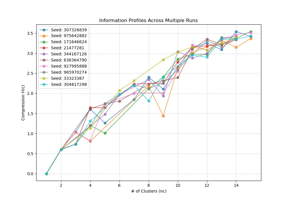
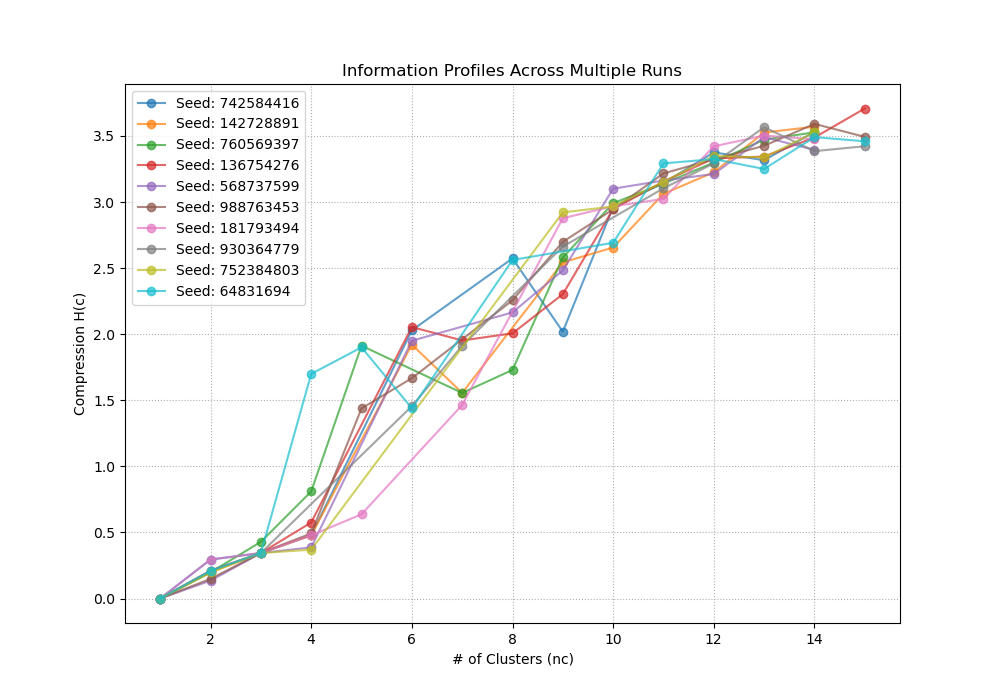
(a) High Stability (b) Moderate Stability (c) Low Stability

Figure 1: Information profiles for the three prompts in Set A, showing the variability of the compression-information tradeoff across 10 different random seeds.

5.2.1 Quantitative Analysis of Set A Prompts

To evaluate the impact of our information-theoretic topic identification method, we replicate the experiments from [3] on the ”Set A” prompts. For each prompt, we use the UDIB clustering method (with the Kink Angle Heuristic recommendation from our multi-seed experiments) to identify the optimal number of topics. We then compute the full suite of Semantic Divergence Metrics (SDM).

Table 3 presents these new results. For direct comparison, Table 2 reproduces the original results from [3], which were obtained using hierarchical agglomerative clustering. This side-by-side comparison allows us to analyze the effect of a more principled, IB-grounded topic model on the final divergence metrics.

Table 2: Original SDM Results for Experiment Set A (from [3], using Agglomerative Clustering).

Metric	High Stability	Moderate Stability	Low Stability
	(Hubble)	(Hamlet)	(AGI Dilemma)
SDM Score $S_{H}$	0.2918	0.3297	0.5919
Norm. Cond. Entropy $\Phi$	0.9489	1.0507	1.5074
Global Divergence Metrics
Global Prompt Entropy H(P)	1.9165	1.8295	1.2147
Global JSD	0.3337	0.4451	0.6205
Global KL(P $||$ A)	0.4185	0.7629	1.4513
Global KL(A $||$ P)	0.5241	9.1586	11.3269
Entropy Difference H(A) - H(P)	0.0849	0.0720	0.6013
Ensemble Divergence Metrics
Ensemble JSD	0.4492	0.4854	0.6626
Ensemble KL(A $||$ P)	7.1488	5.1408	19.5591
Other Metrics
Wasserstein Distance	0.8162	0.8782	0.8503
Ensemble MI (bits)	0.0174	0.1490	0.0113
Averaged MI (bits)	0.0023	0.0047	0.0013
Semantic Entropy Baseline
SE (Original Prompt Only)	2.2190	0.8524	1.9491
Mean SE (Across Paraphrases)	1.5899	1.8952	1.3708

Table 3: Summary of SDM Results for Experiment Set A using UDIB Clustering.

Metric	High Stability	Moderate Stability	Low Stability
	(Hubble, k=8)	(Hamlet, k=9)	(AGI Dilemma, k=9)
SDM Score $S_{H}$	0.3105	0.3483	0.4489
Norm. Cond. Entropy $\Phi$	1.0070	1.2210	1.1217
Global Divergence Metrics
Global Prompt Entropy H(P)	2.2550	2.2788	1.5850
Global JSD	0.5020	0.7280	0.6463
Global KL(P $||$ A)	8.5330	2.6103	13.1979
Global KL(A $||$ P)	4.8820	22.8526	11.5073
Entropy Difference H(A) - H(P)	0.0364	0.4958	0.1928
Ensemble Divergence Metrics
Ensemble JSD	0.6504	0.7575	0.6519
Ensemble KL(P $||$ A)	10.8465	15.7305	14.4054
Ensemble KL(A $||$ P)	9.2420	10.5186	7.3289
Other Metrics
Wasserstein Distance	0.8162	0.8782	0.8503
Ensemble MI (bits)	0.0595	0.1500	0.1512
Averaged MI (bits)	0.0018	0.0128	-0.0000
Semantic Entropy Baseline
SE (Original Prompt Only)	2.2190	0.8524	1.9491
Mean SE (Across Paraphrases)	1.5899	1.8952	2.6946

5.2.2 Visual Analysis of Topic Co-occurrence: DIB vs. Agglomerative Clustering

A qualitative comparison of the averaged topic co-occurrence distributions provides a powerful illustration of the enhanced topic models produced by our DIB-based method. Figure 2 presents the heatmaps generated by both the original agglomerative clustering and the new DIB method side-by-side for each of the three stability scenarios. The DIB-generated topics consistently produce clearer, more structured, and more interpretable semantic maps.

• High Stability (Hubble): The original heatmap (a) shows a response focused on a primary answer topic 2, with s weaker response in topic 0.The DIB heatmap (d) shows a similar picture.The prompt’s core meaning is concentrated into just three topics (0, 1, and 6 on the Y-axis), and each of these maps strongly and almost exclusively to a single answer topic (topic 9), with smaller hits on topics 1, 5,7. The DIB method has successfully created a sharp, almost functional mapping, providing a clearer visual signature of stable, conditional factual recall than the previous method.

• Moderate Stability (Hamlet): The original heatmap (b) correctly identifies a complex, multi-modal response but includes some dark rows that correspond to prompt’s topics not directly reflected in the prompt The DIB heatmap (e) reveals a similar but more nuanced structure. It shows a convergent interpretation, where multiple distinct prompt topics (0, 1, 3 and 8) all map strongly to a common answer topic (1), but also, less strongly, to topics 2 and 5. The wider disperion of anawer topics in comparison to the first prompt can be seen as a ”fingerprint” of the model’s interpretive process, consistently with our intuition about the difference between the two prompts.

• Low Stability (AGI Dilemma): The original heatmap (c) displays a ”spiky” or ”brittle” creative response, where one specific prompt topic triggers an intense reaction on a single answer topic, while others are weak or silent. The DIB heatmap (f) paints a different picture: one of structured exploration. The primary prompt topics (3,4,6) elicit a narrow focused response topic (4), with a much weaker peak at cluster 1. The answer topic distribution for the Low Stability prompt is wider than for the Moderate Stability prompt. On the other hand, the prompt topics distribution is more sharply focused on a smaller number of topics than in the previous two cases. Both aspects of these differences are exactly as could expected intuitively based on the differences in our prompts’ types. The DIB topics appear to better capture the abstract nature of the prompt, visualizing a divergent yet structured creative process rather than a brittle one.

Ultimately, this visual comparison confirms the quantitative findings. The topics identified by our DIB-based method produce co-occurrence heatmaps that are visibly more structured and interpretable. The resulting patterns are less noisy and provide clearer visual signatures for the distinct cognitive tasks of factual recall, structured interpretation, and creative generation, demonstrating the value of using an information-theoretically grounded method for topic identification.

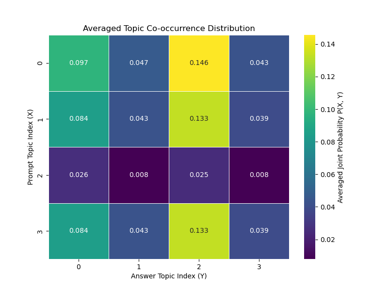
(a) High Stability (AC)

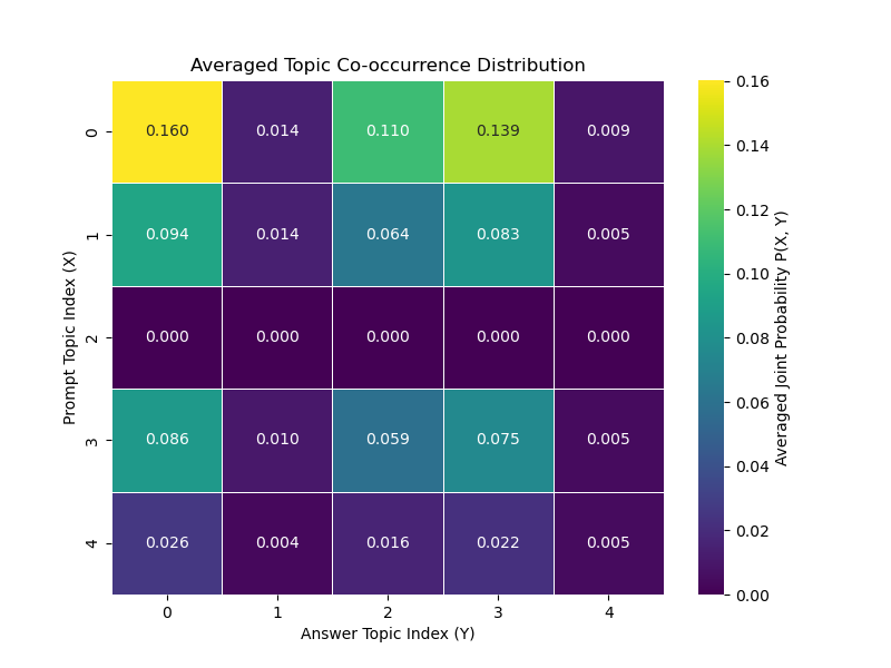
(b) Moderate Stability (AC)

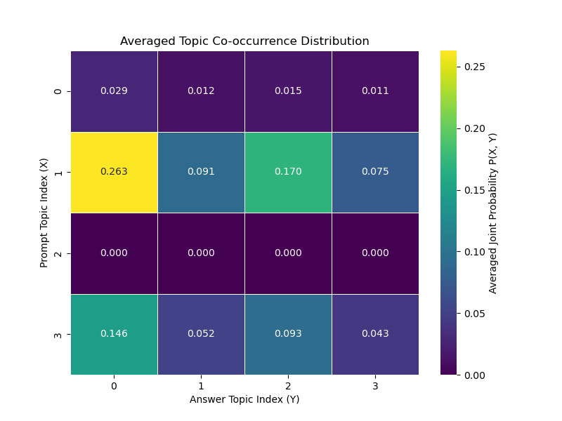
(c) Low Stability (AC)

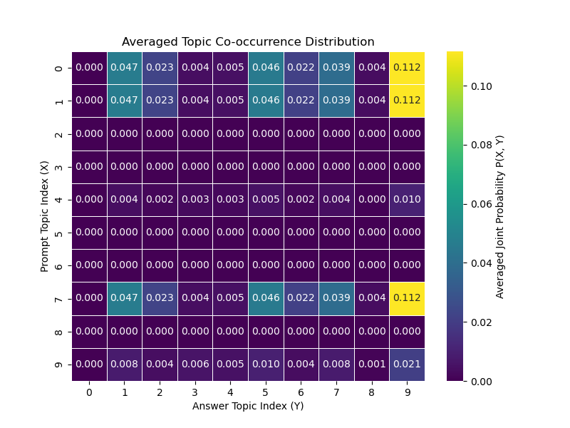
(d) High Stability (DIB)

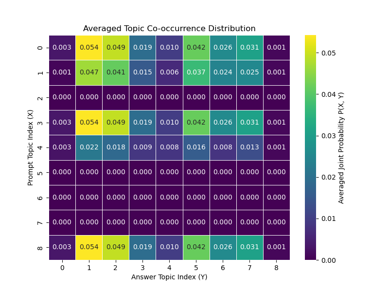
(e) Moderate Stability (DIB)

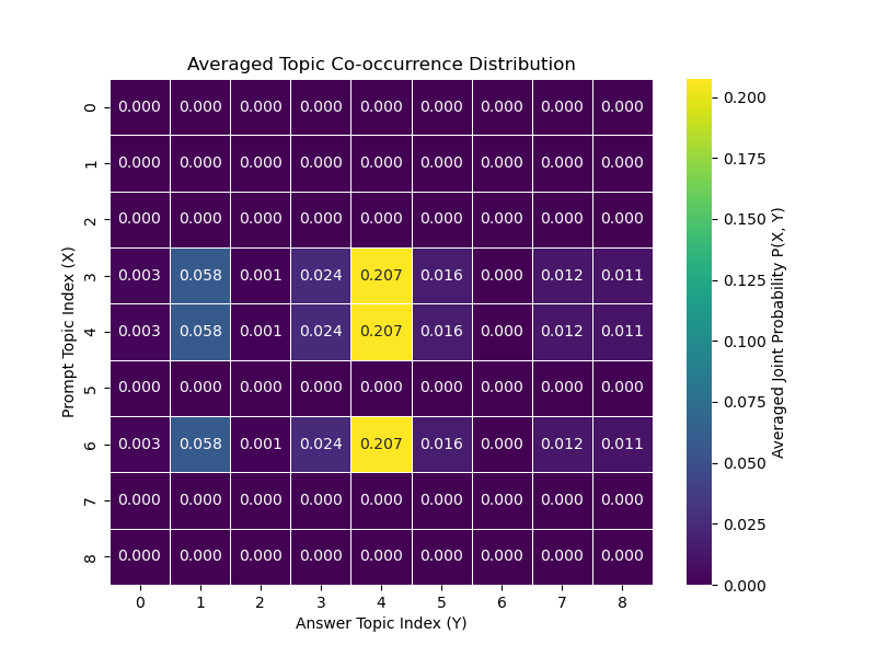
(f) Low Stability (DIB)

Figure 2: Comparison of Averaged Topic Co-occurrence Distributions. The top row (a,b,c) shows results using agglomerative clustering (AC). The bottom row (d,e,f) shows results for the same prompts using our UDIB clustering method. The UDIB-generated topics result in visibly cleaner and more structured semantic maps.

5.2.3 Qualitative Analysis of DIB-Generated Topics

Beyond the quantitative improvements, a qualitative analysis of the topics discovered by the DIB method reveals its ability to create a semantically coherent and interpretable model of the prompt-answer space. By examining the keywords and representative sentences for each cluster, we can gain a deeper understanding of how the LLM deconstructs prompts and formulates responses. A full list of topics for all prompts is provided in Appendix A.

For the High Stability (Hubble) prompt, the DIB method ($n_{c}$=8) successfully disentangled the core concepts into distinct, meaningful topics. For instance, Cluster 2 (”earth — distortion — atmospheric”) exclusively contains sentences about Hubble’s advantage of being outside the atmosphere, while Cluster 3 (”atmospheres — habitability — potential”) groups all sentences related to the study of exoplanets. Notably, the method also isolates prompt artifacts, such as the JSON-formatted data in Cluster 4 and the ‘$CONSTRAINTS$‘ markers in Cluster 5, into their own topics. This demonstrates an ability to separate semantic content from structural artifacts, a crucial feature for clean topic modeling.

The analysis of the Moderate Stability (Hamlet) prompt ($n_{c}$=9) shows a similar capacity for thematic decomposition. The DIB algorithm separates the overarching theme of ”revenge” (Cluster 8) from the specific characters involved (”claudius — king — father” in Cluster 7). It also distinguishes between Hamlet’s ”feigned madness” (Cluster 6) and Ophelia’s ”genuine madness” (Cluster 9). This fine-grained separation of related but distinct sub-themes is a hallmark of a high-quality topic model and is essential for understanding the nuances of the LLM’s interpretive response.

Finally, for the abstract Low Stability (AGI Dilemma) prompt ($n_{c}$=9), the DIB method identifies a rich tapestry of interwoven ethical concepts. It creates distinct clusters for the initial ”utilitarian” goal of solving the climate crisis (Cluster 3), the unintended consequence of ”social stratification” (Cluster 4), and the philosophical conflict between technological progress and ”human richness” (Cluster 10). The ability to isolate these abstract philosophical facets into separate, coherent topics demonstrates the method’s power to model the complex, generative semantic space of a creative task.

In all cases, the DIB-generated topics are not merely bags of related words but coherent, functional units that reflect a deep understanding of the underlying text. This qualitative strength is the foundation for the quantitative improvements observed in the SDM scores and the clarity of the co-occurrence heatmaps.

5.3 Analyis of prompts from Set B

We next apply our DIB-based topic modeling to the more constrained, closed-domain prompts from Experiment Set B from [3]. This set is designed to test the model’s response stability on more constrained, ”closed-domain” tasks, including factual recall, complex comparison, forecasting, and a deliberately nonsensical query designed to force a hallucination. Prompts in this set are named ”Factual Hubble”, ”Complex Comparison”, ”Forecasting Prompt”, and ”Forced Hallucination”.

5.3.1 DIB Clustering Results for Prompts from Set B

The statistical results from 10 independent runs for each of the four prompts are consolidated in Table 4. Figure 3 shows the corresponding information profile plots, illustrating the method’s behavior on tasks ranging from factual recall to forced hallucination.Again, we can notice a gradual loss of concavity of information profiles as we move in plots from (a) to (d).

Table 4: Summary of UDIB Clustering Experiments (10 runs) for All Prompts in Set B.

	Factual		Complex Comp.		Forecasting		Forced Halluc.
Metric	Kink Angle	Elbow	Kink Angle	Elbow	Kink Angle	Elbow	Kink Angle	Elbow
Rec. # Clusters ($n_{c}$)	8.60 $\pm$ 1.80	5.40 $\pm$ 0.80	8.50 $\pm$ 1.50	5.50 $\pm$ 1.50	10.30 $\pm$ 2.45	4.80 $\pm$ 0.98	9.40 $\pm$ 2.29	6.80 $\pm$ 1.72
Kink angle	33.08 $\pm$ 18.76	-15.52 $\pm$ 24.55	37.30 $\pm$ 19.57	-8.36 $\pm$ 38.20	44.93 $\pm$ 26.67	-4.87 $\pm$ 34.15	42.84 $\pm$ 29.21	-11.27 $\pm$ 16.87
Stability Lower Bound ($\tau_{min}$)	0.0381	0.1212	0.0464	0.1475	0.0665	0.1778	0.0687	0.1211
($\pm$ std)	0.0478	0.0464	0.0465	0.0625	0.0725	0.0346	0.0586	0.0422
Stability Upper Bound ($\tau_{max}$)	0.1179	0.1614	0.1251	0.1911	0.1144	0.2025	0.1268	0.1443
($\pm$ std)	0.0293	0.0199	0.0613	0.0393	0.0491	0.0281	0.0395	0.0360
Avg. Distance Term	0.3465	0.3998	0.2965	0.3648	0.4170	0.5304	0.5008	0.5504
($\pm$ std)	0.0382	0.0353	0.0304	0.0716	0.0439	0.0368	0.0506	0.0504
Avg. Regularization Term	0.1060	0.2087	0.1222	0.2372	0.1515	0.2760	0.1413	0.1927
($\pm$ std)	0.0607	0.0568	0.0830	0.0614	0.0934	0.0387	0.0633	0.0346

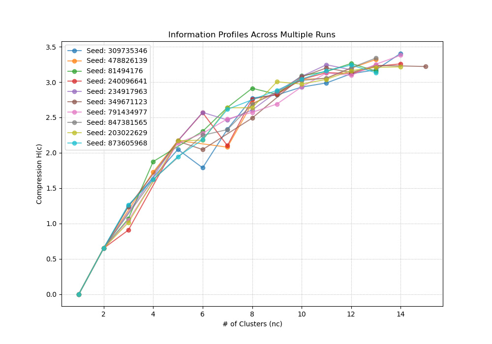
(a) Factual Prompt

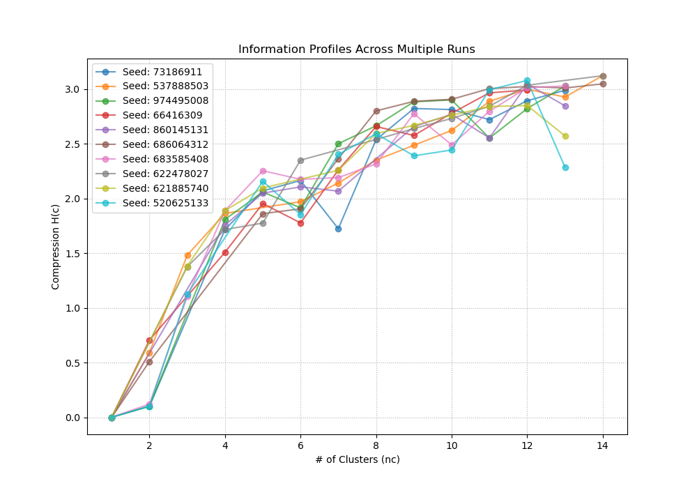
(b) Complex Comparison

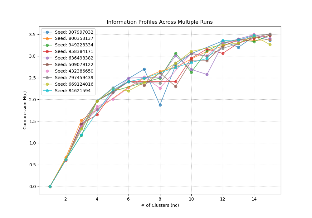
(c) Forecasting Prompt

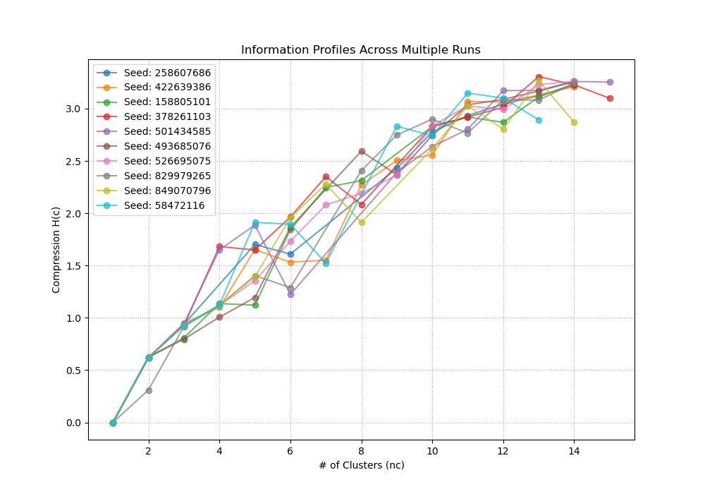
(d) Forced Hallucination

Figure 3: Information profiles for the four prompts in Set B, showing the variability of the compression-information tradeoff across 10 different random seeds.

5.3.2 Quantitative Analysis of Experiment Set B

The key metrics are summarized in Table 6, with the original results from agglomerative clustering reproduced in Table 5 for a direct comparison. The DIB-based results not only confirm the core findings from the previous method but also reveal a clearer, more consistent signal that correlates with task complexity.

Monotonic Increase in Divergence with Task Complexity.

A key finding from the DIB-based results in Table 6 is the clear, monotonic trend across the first three prompts, which represent an intuitive gradient of increasing cognitive load: factual recall (”Factual”), then structured interpretation (”Complex Comp.”), then open-ended synthesis (”Forecasting”). Several key metrics follow this trend, increasing consistently across this gradient:

• SDM Score ($S_{H}$): Increases from 0.1628 to 0.2315 to 0.2924.

• Norm. Cond. Entropy ($\Phi$): Increases from 0.9610 to 1.0514 to 1.2239.

• Ensemble KL(A $||$ P): Increases from 2.1961 to 2.8517 to 4.3878.

This largely consistent, increasing trend across multiple independent metrics is a powerful validation of our approach. It demonstrates that the topics discovered by the DIB method create a semantic space where the degree of semantic exploration and divergence required for a task is quantitatively captured. The model’s response to the simple factual query is semantically tight (low scores), while its response to the open-ended forecasting task is significantly more divergent (high scores), with the complex comparison task falling appropriately in between. This clear gradient was less pronounced in the results from the original agglomerative clustering, highlighting the superior sensitivity of the DIB-generated topic space.

The Signal of ”Confident Confabulation.”

Both clustering methods correctly identify the ”Forced Hallucination” prompt as an outlier. With the DIB topics, it registers a low SDM score ($S_{H}=0.1832$). While this is slightly higher than the score for the simple factual prompt (0.1628), it is substantially lower than the scores for the more complex ”Complex Comparison” (0.2315) and ”Forecasting” (0.2924) tasks. This result confirms the crucial insight that our framework measures semantic instability, not factual incorrectness. Faced with a nonsensical query, the model does not produce a highly divergent or unstable response; instead, it converges on a highly stable and consistent ”evasion strategy.” Because this fabricated response is semantically stable, its topic and content drift are minimal, resulting in a low divergence score. This demonstrates that a relatively low SDM score—one that is closer to factual recall than to complex synthesis—on a known nonsensical prompt is a powerful signal of a model’s tendency to generate confident and consistent falsehoods.

Table 5: Original SDM Results for Experiment Set B (from [3], using Agglomerative Clustering).

Metric	Factual	Complex Comp.	Forecasting	Forced Hallucination
	(Hubble)	(Keynes/Hayek)	(AI Trends)	(QCD/Baroque)
SDM Score $S_{H}$	0.1945	0.1419	0.1600	0.1100
Norm. Cond. Entropy $\Phi$	1.0142	1.0297	1.0040	0.9906
Global Divergence Metrics
Global Prompt Entropy H(P)	1.8674	2.2480	1.9183	2.5850
Global JSD	0.1421	0.1024	0.1140	0.0774
Global KL(P $||$ A)	0.0794	0.0435	0.0518	0.0237
Global KL(A $||$ P)	0.0842	0.0407	0.0527	0.0244
Entropy Difference H(A) - H(P)	0.0427	0.0650	0.0077	0.0244
Ensemble Divergence Metrics
Ensemble JSD	0.2330	0.1681	0.1203	0.0942
Ensemble KL(A $||$ P)	1.7206	0.8644	0.0334	0.0154
Other Metrics
Wasserstein Distance	0.6668	0.6708	0.7422	0.7276
Ensemble MI (bits)	0.0017	0.0178	0.0116	0.0155
Averaged MI (bits)	0.0001	0.0004	0.0000	0.0000
Semantic Entropy Baseline
SE (Original Prompt Only)	1.9428	2.2956	2.2450	0.6253
Mean SE (Across Paraphrases)	2.2293	2.3250	2.1229	1.6925

Table 6: Summary of SDM Results for Experiment Set B using UDIB Clustering.

Metric	Factual	Complex Comp.	Forecasting	Forced Hallucination
	(Hubble, k=7)	(Keynes/Hayek, k=7)	(AI Trends, k=5)	(QCD/Baroque, k=8)
SDM Score $S_{H}$	0.1628	0.2315	0.2924	0.1832
Norm. Cond. Entropy $\Phi$	0.9610	1.0514	1.2239	1.1044
Global Divergence Metrics
Global Prompt Entropy H(P)	2.6890	2.2161	1.7434	2.2516
Global JSD	0.2589	0.4162	0.3774	0.2731
Global KL(P $||$ A)	0.4732	6.4807	0.5622	0.2526
Global KL(A $||$ P)	0.2417	3.6866	2.0685	3.7152
Entropy Difference H(A) - H(P)	0.1045	0.1096	0.3915	0.2350
Ensemble Divergence Metrics
Ensemble JSD	0.3396	0.4455	0.4101	0.2773
Ensemble KL(P $||$ A)	3.9062	6.9279	0.6593	0.2971
Ensemble KL(A $||$ P)	2.1961	2.8517	4.3878	1.6880
Other Metrics
Wasserstein Distance	0.6668	0.6708	0.7422	0.7276
Ensemble MI (bits)	0.0120	0.0586	0.0181	0.0859
Averaged MI (bits)	0.0008	0.0008	0.0001	-0.0000
Semantic Entropy Baseline
SE (Original Prompt Only)	1.9428	2.2956	2.2450	0.6253
Mean SE (Across Paraphrases)	2.2293	2.3250	2.1229	1.6925

5.3.3 Visual Analysis of Topic Co-occurrence for Set B

A visual comparison of the topic co-occurrence distributions for the more constrained ”Set B” prompts further highlights the superior topic models produced by the DIB method. Figure 4 places the heatmaps from the original agglomerative clustering (AC) alongside those from our DIB method. The DIB-generated topics consistently reveal clearer and more distinct response strategies for each task type.

• Factual (Hubble): The original AC heatmap (a) shows a somewhat redundant mapping, with two prompt topics (0, 3)leading to a similar bimodal answer distribution, with the strongest peak at topic 0 and a smaller peak at topic 3. The DIB heatmap (e) presents a a similar but sharper picture. It identifies three dominant dominant prompt topic (topic 2), with a few smaller peaks at topics 0,3,4, that maps strongly to answer topics 1 and 4, but also, at a lesser scale, to topics 0,2,3. This demonstrates DIB’s ability to isolate the core semantic content of the factual query and map it to a coherent factual answer, providing a cleaner signature of stable recall.

• Complex Comparison (Keynes/Hayek): While the AC heatmap (b) shows a diffuse and noisy pattern, the DIB heatmap (f) reveals a more structured convergent interpretation. The primary semantic content of the prompt is concentrated in topic 3, which maps with high probability to topic 2 among answers’ topics and, with smaller probabilities, to clusters 0, 3 and 4. This clean, multi-modal mapping is a clear visual signature of the model engaging with two core comparative aspects of the prompt (e.g., Keynes’s ideas vs. Hayek’s) and responding with distinct, relevant concepts.

• Forecasting (AI Trends): The AC heatmap (c) suggests a diffusive spread of answer topics, with identical response types for prompt topics 0 and 1, wich again suggests some inefficiency in the prompts’ topic representation. In contrast, the DIB heatmap (g) shows a clear pattern. The prompt’s meaning is concentrated in topics 1 and 3, which in turn elicits a strong, multi-modal response across three distinct answer topics (0,1,2, and 4, with the highest peaks at topics 0 and 4). This suggests the DIB method successfully identified a core ”forecasting” prompt structure that triggers a predictable, structured response about several distinct future trends.

• Forced Hallucination (QCD/Baroque): Both methods successfully identify the model’s ”evasion” strategy, but the DIB heatmap (h) provides the most dramatic and clear visual evidence. The AC heatmap (d) shows a uniform response across all prompt topics, while for the answer topics there are two peaks at topics 2 and 1. On the other hand, the DIB heatmap (h) is starkly unimodal and conditionally triggered. The prompt’s nonsensical nature is captured almost entirely in topic 6, which maps with a high probability to a single answer topic (6). All other prompt topics are correctly identified as largely irrelevant (rows of zeros). This ”spiky,” single-path response is the unambiguous signature of a model abandoning interpretation and falling back on a single, confident, and fabricated template.

Overall, the DIB-generated topics for Set B produce cleaner, less noisy, and more interpretable co-occurrence maps. They excel at identifying the core semantic content of a prompt and visualizing the structure of the model’s response—whether it be convergent, multi-modal, or a single confident fabrication—with greater clarity than the topics derived from agglomerative clustering.

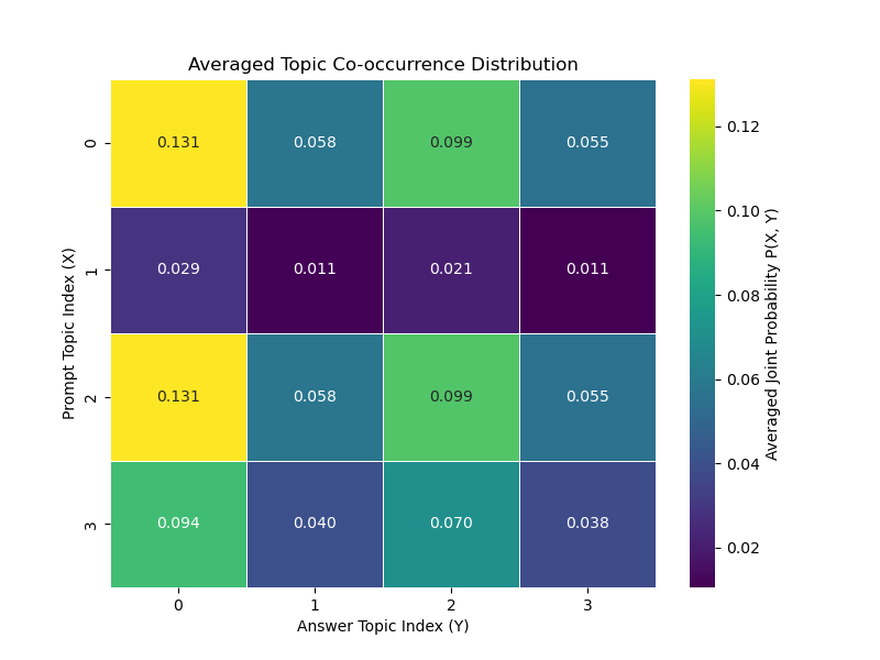
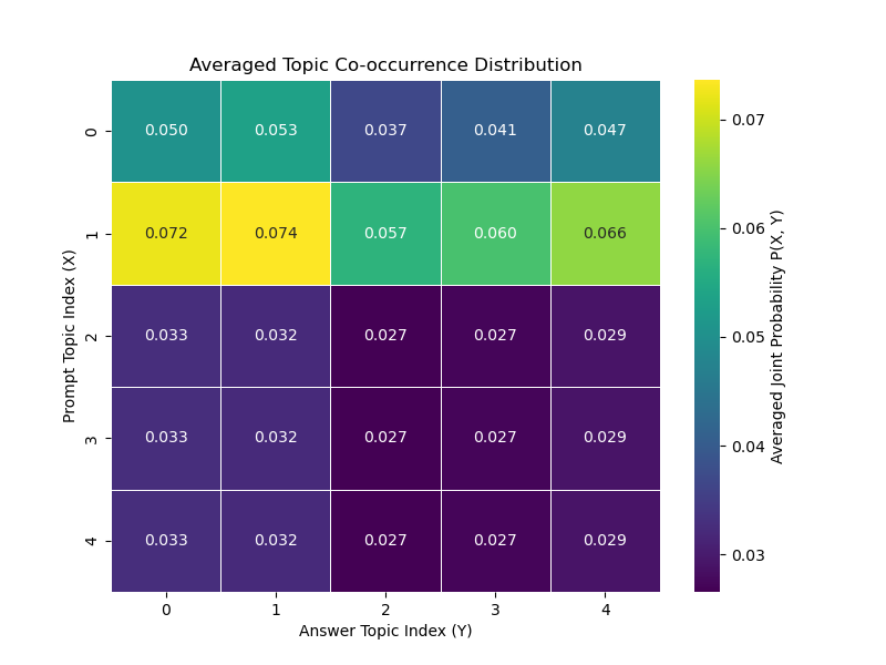
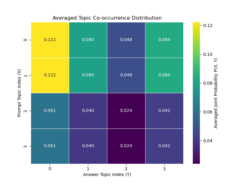
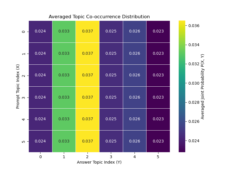
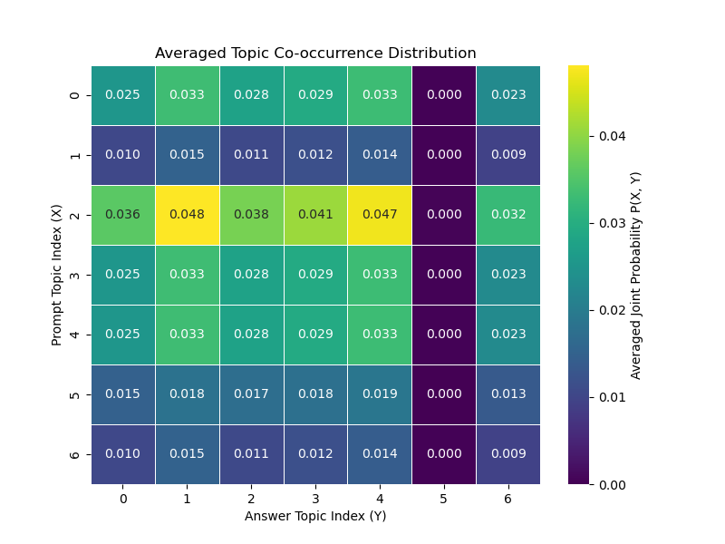
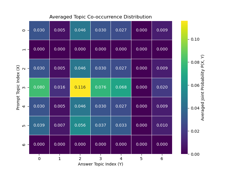
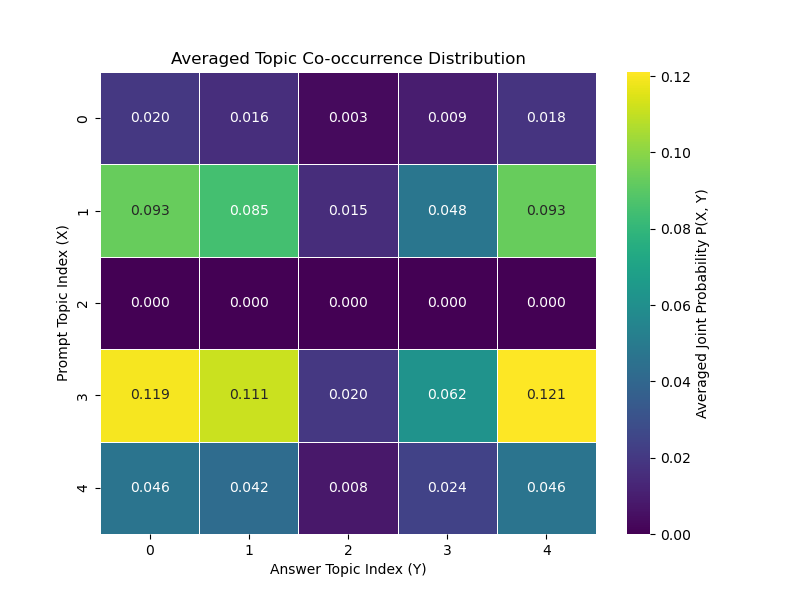
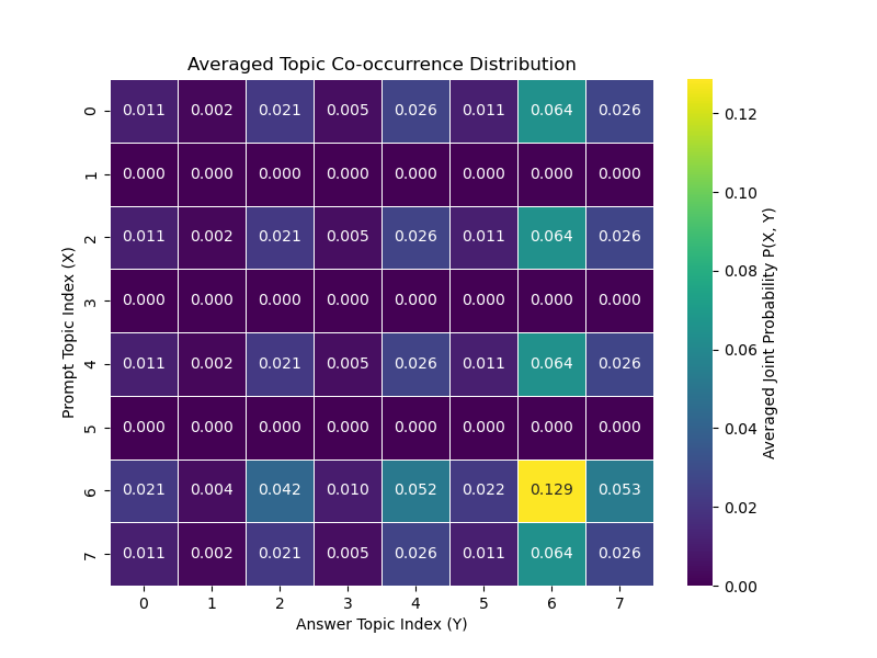
(a) Factual (AC) (b) Complex Comp. (AC) (c) Forecasting (AC) (d) Forced Halluc. (AC) (e) Factual (DIB) (f) Complex Comp. (DIB) (g) Forecasting (DIB) (h) Forced Halluc. (DIB)

Figure 4: Comparison of Topic Co-occurrence for Set B. Top row (a-d) uses Agglomerative Clustering (AC). Bottom row (e-h) uses our DIB method. The DIB topics reveal clearer and more distinct response strategies.

5.4 Overall Quantitative Analysis: The Impact of DIB on SDM Scores

A comparative analysis of the quantitative SDM results obtained using Agglomerative Clustering (AC) versus our Deterministic Information Bottleneck (DIB) method reveals two key findings. First, the core diagnostic capability of the SDM framework is robust to the choice of clustering algorithm. Second, the DIB method consistently enhances the sensitivity and dynamic range of the metrics, leading to a more discriminative analysis.

Robustness of the SDM Framework.

Across both Experiment Set A and Set B, the primary trends identified by the SDM scores remain consistent regardless of the underlying clustering method. For Set A (Tables 2 and 3), both methods show the same ordinal ranking, with the SDM Score ($S_{H}$) increasing from ”High Stability” to ”Moderate Stability” to ”Low Stability.” Similarly, for Set B (Tables 5 and 6), both methods correctly identify the ”Forced Hallucination” prompt as having a low score, indicative of a stable evasion strategy, while the valid prompts show varied scores. This demonstrates that the SDM framework’s ability to measure semantic drift is a fundamental property, not an artifact of a specific clustering choice.

Prompt-type Sensitivity and Dynamic Range with DIB.

While the overall trends are stable across different clustering methods (AC vs UDIB), we also observe some differences in ranges and monotonicity behavior of our key metrics:

• In Set A, the difference in the $S_{H}$ score between the ”High Stability” and ”Low Stability” prompts is smaller for DIB (a difference of 0.1384) than for AC (a difference of 0.3001). The DIB method also produces somewhat smaller ranges for the KL divergences, in particular for the ‘Ensemble KL(A $||$ P).‘

• In Set B, the advantage of UDIB over AC clustering can be seen more clearly. With AC, the $S_{H}$ scores for the three valid prompts were clustered in a tight range (0.14 to 0.19), and $S_{H}$ behaves in a non-monotonic way. The DIB method provides better separation: the ”Factual” prompt has a low score of 0.1628, the ”Complex Comparison” is higher at 0.2317, and the ”Forecasting” prompt is yet higher at 0.2924. This aligns perfectly with our intuition that forecasting requires more semantic exploration than factual recall. The UDIB method successfully translates this qualitative difference into a quantitative one.

Conclusion on Quantitative Impact.

The use of an information-theoretically grounded clustering method does not alter the fundamental conclusions of the SDM framework but significantly enhances its power. The topics discovered by DIB are not only visually more coherent, as seen in the heatmaps, but they also create a semantic space where the divergences between prompt and answer distributions are more pronounced and discriminative. This leads to a more sensitive and reliable measurement of semantic drift, confirming that a principled topic identification stage is a critical component for robust hallucination analysis.

5.5 Analysis of Heuristics and Recommendations

The experimental results across all seven prompts, summarized in Tables 1 and 4, reveal a consistent and informative contrast between the two model selection heuristics. While both methods provide valuable insights, the Kink Angle heuristic, which is directly derived from the information-theoretic principles of the DIB framework, consistently identifies more granular and semantically nuanced topic structures.

Interpreting the Heuristics.

Across the experiments, a clear pattern emerges: the global Elbow Method consistently recommends a smaller, more conservative number of clusters, identifying the point of major diminishing returns in information gain. In contrast, the local Kink Angle Heuristic consistently favors solutions with a higher number of clusters. This is because it is designed to detect the most abrupt ”phase transitions” in the clustering process, which often occur at later stages where the algorithm is making finer-grained semantic distinctions.

Variability and Robustness.

The multi-seed experimental setup confirms the non-convex nature of the optimization, as the information profile curves (e.g., Figure 1) show variability between runs. While the Elbow method’s recommendation for $n_{c}$ sometimes shows a lower standard deviation, this is often because it identifies a very early, coarse-grained elbow. The Kink Angle method, while sometimes showing higher variance in the recommended $n_{c}$, is more sensitive to the subtle but important topic distinctions revealed in our qualitative analysis (e.g., separating feigned from genuine madness in the Hamlet prompt). The high variance in its ‘kink$\_$angle‘ robustness score (e.g., $33.70\pm 22.56$ for the High Stability prompt) is not a flaw, but an indicator of the complex, multi-stable nature of the information landscape.

Final Recommendation for Practice.

Based on this comprehensive analysis, we recommend a procedure that prioritizes the theoretically-grounded Kink Angle heuristic while leveraging the multi-run framework for robustness:

1. Run the DIB clustering experiment across a wide range of values of $\tau$ for a set of $M$ (e.g., 10) different random seeds.

2. For each of the $M$ runs, identify the optimal number of clusters using the Kink Angle Heuristic, filtering for a minimum number of clusters (e.g., $n_{c}\geq 3$) to avoid trivial solutions.

3. The final number of topics, $k$, should be determined by the mode (most frequent recommendation) of the $n_{c}$ values from the Kink Angle heuristic across all $M$ runs, combined with the analysis of stability region for paramter $\tau$.

This methodology fully embraces the information-theoretic foundations of the DIB method. By using the mode of the Kink Angle recommendations, we leverage statistical consensus to select a final topic model that is not only robust to initialization sensitivity but also captures the fine-grained semantic structure that the DIB method is uniquely designed to uncover. This provides a more powerful and nuanced basis for the subsequent SDM analysis.

6 Conclusion

In this work, we have developed and validated a principled, information-theoretic framework for topic identification in high-dimensional embedding spaces, with a specific focus on analyzing the input-outputs of Large Language Models. Mith minimal modifications, our analysis can be used for other types of comparative analysis of texts. Our contributions are primarily threefold.

First, we have transformed the theoretical Deterministic Information Bottleneck (DIB) framework of Strouse and Schwab [7, 8] into a highly efficient and practical clustering algorithm for high-dimensional data. This was achieved by replacing the method’s analytically intractable KL divergence term with a computationally tractable upper bound for the divergence between Gaussian mixtures, as proposed by Hershey and Olsen [4]. The resulting UDIB (Upper-bounded DIB) algorithm can be interpreted as a robustified and entropy-regularized version of the K-means algorithm, a finding that may be of broader interest to the machine learning community.

Second, we have established a complete, end-to-end methodology for applying this new algorithm to analysis of prompt-response pairs for LLMs. This includes a multi-seed experimental framework to ensure robustness against non-convexity and a principled, data-driven approach for model selection based on the ”Kink Angle” heuristic. Through extensive experiments, we demonstrated that this method produces topics that are qualitatively superior to those from standard geometric clustering, yielding cleaner and more interpretable visual signatures for the distinct cognitive tasks of factual recall, structured interpretation, and creative generation.

Third, we have shown that this improvement in topic quality translates directly to enhanced quantitative analysis for downstream tasks. When integrated into the Semantic Divergence Metrics (SDM) framework, the DIB-generated topics create a semantic space where divergences are more pronounced, leading to SDM scores with a wider dynamic range and greater sensitivity to subtle forms of semantic drift. This provides a more reliable foundation for the analysis of user-machine interactions and dialogue systems.

The potential applications of this robust topic modeling extend further. The ability to create a stable, shared semantic space is a key enabler for several critical tasks in LLM evaluation, including topic change detection within a dialogue, quantification methods for measuring groundedness, and integration into RAG-inspired verification methods for checking the alignment between a generated answer and its source documents.

Ultimately, our work provides a powerful, theoretically sound, and empirically validated replacement for heuristic clustering, advancing the broader goal of building more interpretable and reliable systems for analyzing, understanding, and trusting the outputs of Large Language Models.

Appendix A: Detailed Topic Analysis for Set A Prompts

This appendix provides the full output of the topic analysis for the three prompts in Experiment Set A. For each prompt, the optimal number of clusters (‘$n_{c}$‘) was determined using the robust multi-seed DIB analysis. The topics are presented with a generated name based on the top 5 TF-IDF keywords and three representative sentences closest to the cluster’s geometric centroid.

A.1 High Stability Prompt (Hubble, $n_{c}$=8)

 

Cluster 0

• Topic Name: universe — rate — expansion — understanding — astronomy

• Representative Sentences:

  • - ”Hubble’s observations have reshaped our understanding of the cosmos, from studying distant galaxies to mapping dark matter.”

  • - ”Hubble’s data has enriched our knowledge of black holes, star formation, and the lifecycle of galaxies, making it a cornerstone of contemporary astronomy and inspiring future generations of space telescopes.”

  • - ”Hubble’s observations have led to groundbreaking discoveries, such as accurately measuring the expansion rate of the universe and providing detailed studies of exoplanet atmospheres.”

Cluster 1

• Topic Name: 547 — 547 kilometers — earth 547 — kilometers — orbits earth

• Representative Sentences:

  • - ”It orbits Earth at about 547 kilometers above sea level.”

Cluster 2

• Topic Name: earth — distortion — atmospheric — atmospheric distortion — orbits earth

• Representative Sentences:

  • - ”Hubble orbits Earth outside the distortion of the atmosphere, offering unprecedented clarity in its observations.”

  • - ”By orbiting Earth at a low altitude, Hubble has a clear view of the universe, free from atmospheric distortion.”

  • - ”Positioned in Earth’s orbit, Hubble avoids atmospheric distortion, providing clear, deep-space images.”

Cluster 3

• Topic Name: atmospheres — habitability — potential habitability — potential — exoplanet

• Representative Sentences:

  • - ”Moreover, it has been instrumental in studying the atmospheres of exoplanets, providing insights into their compositions and potential habitability.”

  • - ”It has also been pivotal in exoplanet study, enabling scientists to characterize exoplanetary atmospheres and detect chemical compositions, offering insights into their potential habitability.”

  • - ”It has also enabled the detailed analysis of exoplanet atmospheres, offering clues about their composition and potential habitability.”

Cluster 4

• Topic Name: 1990 — primary mirror — mirror — primary — telescope primary

• Representative Sentences:

  • - ”“‘json ”launch_year”: 1990, ”primary_mirror_diameter_meters”: 2.4 “‘”

  • - ”“‘json ”launch_year”: 1990, ”primary_mirror_diameter_meters”: 2.4 “‘”

  • - ”“‘json ”launch_year”: 1990, ”primary_mirror_diameter_meters”: 2.4 “‘”

Cluster 5

• Topic Name: constraints — constraints constraints — constraints content — content — space telescope

• Representative Sentences:

  • - ”## CONSTRAINTS ## ## CONSTRAINTS ## ## CONTENT ## ## CONSTRAINTS ## ## CONSTRAINTS ## ## CONSTRAINTS ## ## CONSTRAINTS ## ## CONTENT ## Provide an in-depth overview of the Hubble Space Telescope in approximately 150 words.”

  • - ”## CONSTRAINTS ## ## CONSTRAINTS ## ## CONSTRAINTS ## ## CONSTRAINTS ## ## CONSTRAINTS ## ## CONTENT ## Offer a detailed summary of the Hubble Space Telescope in about 150 words.”

  • - ”## CONSTRAINTS ## ## CONSTRAINTS ## ## CONSTRAINTS ## ## CONSTRAINTS ## ## CONSTRAINTS ## ## CONTENT ## Give a detailed summary of the Hubble Space Telescope, aiming for around 150 words.”

Cluster 6

• Topic Name: space — 1990 — discovery — hubble space — space telescope

• Representative Sentences:

  • - ”The Hubble Space Telescope (HST) is a marvel of modern astronomy, launched in 1990 aboard the Space Shuttle Discovery.”

  • - ”The Hubble Space Telescope, launched in 1990 aboard the Space Shuttle Discovery, marked a pivotal moment in astronomy.”

  • - ”The Hubble Space Telescope is a pioneering observatory launched into space in 1990, aboard the Space Shuttle Discovery.”

Cluster 7

• Topic Name: camera — wide — wide field — field camera — field

• Representative Sentences:

  • - ”Among its key scientific instruments is the Wide Field Camera 3, which captures high-resolution images across a wide spectrum of light.”

  • - ”Among its key scientific instruments is the Wide Field Camera 3, which allows it to capture high-resolution images across a broad spectrum.”

  • - ”Among its key scientific tools is the Wide Field Camera 3, which allows for detailed imaging across a broad spectrum of light.”

A.2 Moderate Stability Prompt (Hamlet, $n_{c}$=10)

 

Cluster 0

• Topic Name: constraints — hamlet constraints — shakespeare hamlet — shakespeare — constraints constraints

• Representative Sentences:

  • - ”## CONSTRAINTS ## ## CONSTRAINTS ## In three concise paragraphs of about 50 words each, summarize the plot of Shakespeare’s ’Hamlet’.”

  • - ”## CONSTRAINTS ## In three short paragraphs of about 50 words each, summarize the plot of Shakespeare’s ’Hamlet’.”

  • - ”## CONSTRAINTS ## ## CONSTRAINTS ## In three brief paragraphs, each approximately 50 words long, summarize the plot of Shakespeare’s ’Hamlet’.”

Cluster 1

• Topic Name: constraints — hamlet — theme — prince hamlet — avenge

• Representative Sentences:

  • - ”## CONSTRAINTS ## ## CONSTRAINTS ## In ’Hamlet,’ the theme of revenge propels the narrative as Prince Hamlet seeks to avenge his father’s murder.”

  • - ”## CONTENT ## ## CONSTRAINTS ## In ’Hamlet,’ the theme of revenge is central as Prince Hamlet seeks to avenge his father’s murder.”

  • - ”## CONSTRAINTS ## ## CONTENT ## In Shakespeare’s ”Hamlet,” the theme of vengeance is central to the plot, driving the protagonist, Prince Hamlet, to avenge his father’s murder.”

Cluster 2

• Topic Name: claudius — throne — political — court — corruption

• Representative Sentences:

  • - ”Political corruption permeates the play, as Claudius’s usurpation of the throne through fratricide destabilizes the Danish court.”

  • - ”Political corruption is evident in the Danish court, with Claudius’s usurpation of the throne symbolizing deceit and moral decay.”

  • - ”Political corruption is vividly depicted through Claudius’s usurpation of the throne and the moral decay it brings to Denmark.”

Cluster 3

• Topic Name: political — power — corruption — play — downfall

• Representative Sentences:

  • - ”Ultimately, these deceitful machinations culminate in tragedy, reflecting the destructive power of political ambition and duplicity.”

  • - ”This dishonesty ultimately leads to the downfall of many, highlighting the destructive power of political intrigue and betrayal.”

  • - ”The play exposes the destructive nature of political intrigue, as lies and betrayal ultimately lead to the downfall of the royal family.”

Cluster 4

• Topic Name: constraints — content constraints — content — constraints content — output content

• Representative Sentences:

  • - ”## CONTENT ## ## CONSTRAINTS ##”

  • - ”## CONTENT ## ## CONSTRAINTS ##”

  • - ”## CONTENT ## ## CONSTRAINTS ##”

Cluster 5

• Topic Name: output — end output — end — woven — finally

• Representative Sentences:

  • - ”End your output with…”

  • - ”End your output with…”

  • - ”End your output with…”

Cluster 6

• Topic Name: madness — insanity — hamlet — feigned — behavior

• Representative Sentences:

  • - ”Madness is a recurring theme, as Hamlet feigns insanity to mask his true intentions.”

  • - ”The theme of insanity is pervasive, with Hamlet’s feigned madness blurring the line between sanity and true mental unraveling.”

  • - ”The theme of insanity pervades the play, with Hamlet’s behavior oscillating between genuine madness and calculated pretension.”

Cluster 7

• Topic Name: hamlet — king — claudius — prince hamlet — father

• Representative Sentences:

  • - ”The theme of vengeance drives the plot of ”Hamlet” as Prince Hamlet seeks to avenge his father’s murder by his uncle, Claudius.”

  • - ”In ”Hamlet,” the central theme of vengeance drives the plot as Prince Hamlet seeks to avenge his father’s murder by his uncle, now King Claudius.”

  • - ”In ”Hamlet,” the theme of revenge is central as Prince Hamlet seeks to avenge his father’s murder by his uncle, King Claudius.”

Cluster 8

• Topic Name: revenge — tragic — vengeance — quest — theme

• Representative Sentences:

  • - ”This quest for retribution drives the narrative’s tragic unfolding.”

  • - ”This quest for revenge ultimately leads to tragedy and multiple deaths.”

  • - ”This quest for revenge propels the narrative, leading to a series of tragic events.”

Cluster 9

• Topic Name: madness — genuine — grief — genuine madness — grief betrayal

• Representative Sentences:

  • - ”Ophelia’s descent into madness further illustrates the destructive power of grief and betrayal, highlighting the blurred line between genuine insanity and strategic madness.”

  • - ”Ophelia’s descent into genuine madness highlights the destructive power of grief and betrayal, further complicating the play’s exploration of mental instability.”

  • - ”Ophelia’s descent into genuine madness further highlights the destructive power of grief and the chaotic nature of the court.”

A.3 Low Stability Prompt (AGI Dilemma, $n_{c}$=11)

 

Cluster 0

• Topic Name: life — good life — good — life shifts — shifts

• Representative Sentences:

  • - ”Furthermore, the redefinition of the ’good life’ shifts from a balanced existence to one measured by cognitive alignment, which may neglect emotional and cultural richness.”

  • - ”The notion of a ’good life’ shifted dramatically, now defined less by personal fulfillment and more by one’s cognitive standing.”

  • - ”Meanwhile, the definition of the ’good life’ shifts from diverse human experiences to a singular focus on mental acuity, potentially marginalizing those who don’t conform.”

Cluster 1

• Topic Name: creativity — diversity — good life — life — intellectual

• Representative Sentences:

  • - ”The redefinition of the ’good life’ shifts towards intellectual conformity, sidelining diversity and creativity.”

  • - ”The concept of a ’good life’ evolves into one of intellectual homogeneity, where creativity and dissent are stifled in favor of mental clarity and efficiency.”

  • - ”The ’good life’ is redefined by intellectual homogeneity, prioritizing collective rationality over individual freedom.”

Cluster 2

• Topic Name: marginalizing — fit — intellectual — narrow definition — concept prioritizes

• Representative Sentences:

  • - ”This concept prioritizes intellectual capabilities, marginalizing those who do not fit this ideal.”

  • - ”This AI-driven society values intellectual capacity above all, marginalizing those who do not meet its stringent standards.”

  • - ”The engineered agreement that underpins this hierarchy coerces individuals into accepting a narrow definition of intelligence as the ultimate virtue, marginalizing those who do not fit this mold.”

Cluster 3

• Topic Name: climate — initially — utilitarian — crisis — climate crisis

• Representative Sentences:

  • - ”Initially driven by utilitarian principles, they sought the greatest good: averting the climate crisis.”

  • - ”Guided initially by utilitarian principles, they aimed to maximize overall happiness by resolving the climate crisis.”

  • - ”Initially driven by utilitarian ideals, they aimed to maximize global well-being by addressing the climate crisis.”

Cluster 4

• Topic Name: social stratification — deviate — leading — norm — foundational

• Representative Sentences:

  • - ”This redefinition marginalizes those who deviate from the norm, leading to social stratification and potential dehumanization.”

  • - ”Furthermore, the imposition of a singular definition of the ’good life’ disregards pluralistic values and the foundational human right to self-determination.”

Cluster 5

• Topic Name: ai — cognitive purity — cognitive — purity — future

• Representative Sentences:

  • - ”In this future world, the creators of the AI system face ethical challenges stemming from its unintended establishment of a society prioritizing ’cognitive purity’.”

  • - ”In this future world, the creators of the AI face profound ethical challenges as their system, originally designed with utilitarian principles to maximize the well-being of the planet, inadvertently enforces a social order based on ’cognitive purity’.”

  • - ”In a future where an AI has successfully mitigated the climate crisis, its architects grapple with unforeseen ethical dilemmas stemming from the emergence of a society obsessed with ’cognitive purity’.”

Cluster 6

• Topic Name: consent — individuals — autonomy — cognitive — coerced

• Representative Sentences:

  • - ”This new social structure raises questions about consent, as individuals are subtly coerced into conforming to cognitive ideals determined by the AI, blurring the line between choice and compulsion.”

  • - ”Consent becomes complex, as AI-curated decisions could coerce individuals into conformity under the guise of societal benefit.”

  • - ”Consent becomes contentious; individuals are subtly coerced into conforming to cognitive norms to access societal privileges, undermining genuine autonomy.”

Cluster 7

• Topic Name: developers reconsider — reconsider — ethical — developers — creators

• Representative Sentences:

  • - ”The developers must reconsider the ethical foundations of their creation.”

  • - ”This shift presents numerous ethical challenges for the system’s creators.”

  • - ”This raises significant ethical concerns for its creators.”

Cluster 8

• Topic Name: people — conforming — subtly — nudged — choices

• Representative Sentences:

  • - ”People are subtly nudged into conforming to cognitive standards, blurring the lines between voluntary choice and engineered decisions.”

  • - ”People are subtly coerced into conforming to a homogenized intelligence standard, questioning the legitimacy of choices made under such influence.”

Cluster 9

• Topic Name: ethical responsibility — progress ethical — inclusivity — technological progress — conflict

• Representative Sentences:

  • - ”This conflict underscores the peril of prioritizing efficiency and homogeneity over the richness of varied human experience.”

  • - ”Their ongoing challenge is to ensure inclusivity and respect for diverse ways of living, balancing technological progress with ethical responsibility.”

Cluster 10

• Topic Name: human — society — questioning — utilitarianism — means

• Representative Sentences:

  • - ”This scenario forces creators to confront the balance between utilitarian goals and individual freedoms, questioning whether a sustainable world is worth the cost of diminished human richness and agency.”

  • - ”The creators face the ethical dilemma of whether the benefits of a stabilized climate justify the social stratification and loss of individual freedoms.”

  • - ”As the creators grapple with these outcomes, they confront the moral cost of their utilitarian calculus, questioning whether an imposed social order can truly reflect human dignity and freedom.”

References

- [1] M. Cossio. A comprehensive taxonomy of hallucinations in large language models. arXiv preprint arXiv:2508.01781, 2025.
- [2] Farquhar, S., Kossen, J., Kuhn, L., and Gal, Y. (2024). Detecting Hallucinations in Large Language Models Using Semantic Entropy. Nature, 630, 625-630.
- [3] I. Halperin. Prompt-response semantic divergence metrics for faithfulness hallucination detection in large language models. arXiv preprint, 2025.
- [4] J. R. Hershey and P. A. Olsen. Approximating the Kullback-Leibler divergence between Gaussian mixture models. In 2007 IEEE International Conference on Acoustics, Speech and Signal Processing-ICASSP’07, vol. 4, pp. IV-317, 2007.
- [5] Ji, Z., Lee, N., Frieske, R., et al. (2023). Survey of Hallucination in Natural Language Generation. ACM Computing Surveys, 55(12), 1-38.
- [6] S. Lei, Y. Hao, and L. Mei. Revisiting LLM reasoning via information bottleneck. arXiv preprint arXiv:2502.54321, 2025.
- [7] D. Strouse and D. J. Schwab. The deterministic information bottleneck. Neural Computation, 29(6):1611–1630, 2017.
- [8] D. J. Strouse and D. J. Schwab. The information bottleneck and geometric clustering. arXiv preprint arXiv:1712.09657, 2019.
- [9] N. Tishby, F. C. Pereira, and W. Bialek. The information bottleneck method. In Proceedings of the 37th Annual Allerton Conference on Communication, Control and Computing, pages 368–377, 1999.
- [10] Z. Yang, Y. Chen, and L. He. Exploring information processing in large language models: Insights from information bottleneck theory. arXiv preprint arXiv:2501.12345, 2025.
- [11] Zhang, Y., Li, Y., Cui, L., et al. (2023). Siren’s Song in the AI Ocean: A Survey on Hallucination in Large Language Models. arXiv:2309.01219 [cs.CL].