Quantum Tomography of Suspended Carbon Nanotubes

Abstract

We present an all-mechanical protocol for coherent control and full quantum-state reconstruction of the fundamental flexural mode of a suspended carbon nanotube (CNT). Calibrated impulses from a nearby atomic force microscope (AFM) tip serve a dual role: they implement mechanical $\pi/2$ rotations for Ramsey interferometry and realize phase-space displacements for Wigner function tomography via displaced-parity sampling. The same actuator thus unifies control and tomography while avoiding optical heating and eliminating on-chip microwave drive lines at the resonator. We derive explicit control pulse sequences and a master-equation description that map measured signals onto the energy-relaxation and phase-coherence times, as well as onto parity-based quantum signatures, including negative regions of the Wigner function. The approach is compatible with several readout modalities: direct AFM deflection, dispersive coupling to a Cooper-pair box, and dispersive microwave cavity probing. Together, these techniques provide complete access to populations, coherence, and parity within a single device architecture. This minimal scheme provides a practical route to all-mechanical quantum control and state-resolved characterization of decoherence in mesoscopic mechanical systems.

I I. Introduction

Probing quantum decoherence in mesoscopic mechanical systems is a fundamental challenge for quantum technologies and for tests of macroscopic quantum phenomena [1, 2, 3, 4]. Nanomechanical oscillators provide a natural platform for such investigations because they are highly sensitive to environmental interactions and can exhibit nonclassical behavior [5, 6, 7, 8, 9]. An extensive literature has established the key ingredients for reaching the quantum regime in nanomechanics, including dilution-temperature operation, sideband or feedback cooling, high-$Q$ suspension, and dispersive readout, across optomechanical membranes, bulk-acoustic modes, and phononic crystals. These techniques encompass sideband cooling to the ground state [10], quantum ground-state preparation and single-phonon control [11], ultralong phonon lifetimes in engineered high-$Q$ resonators [12], and measurement-based quantum control of mechanical motion [13].

Within these platforms, suspended carbon nanotubes (CNTs) stand out as some of the lightest high-$Q$ mechanical resonators, with zero-point motion amplitudes $x_{\mathrm{zpf}}$ in the picometer range and large frequency-to-mass ratios [14, 15, 16, 17]. Their small dimensions and strong coupling to external forces enable precise manipulation and detection of vibrational states, which makes them well suited to probing quantum decoherence mechanisms in mechanical systems [18, 19, 20, 21]. Bringing such resonators into the regime of coherent control enables tests of macroscopic quantum behavior and opens opportunities for ultrasensitive force and field sensing.

At present, however, actuation, control, and tomography are often implemented through separate physical channels, for example optical drive with microwave readout, or on-chip microwave control paired with a distinct tomographic protocol [11, 13, 10, 6]. This partitioning poses challenges for experiments at the mesoscopic scale and can introduce additional dissipation [2, 7, 9]. Despite advances in cooling and dispersive sensing, a compact and experimentally simple route to both coherent control and full quantum-state reconstruction of a CNT mechanical mode has remained difficult to achieve.

In this paper, we propose and analyze an all-mechanical protocol that achieves coherent control and tomography of a single suspended CNT. Short, calibrated impulses from a nearby atomic force microscope (AFM) tip serve a dual role: they implement mechanical $\pi/2$ rotations for Ramsey interferometry and realize phase-space displacements for the reconstruction of the Wigner function via displaced-parity sampling. This purely mechanical actuation avoids optical heating and eliminates on-chip microwave drive lines at the resonator, while retaining nanometer-scale spatial selectivity and sub-femtonewton scale force resolution. The readout is compatible with three complementary transducers: direct AFM deflection, dispersive coupling to a Cooper-pair box (CPB), and dispersive microwave cavity probing, allowing single-mode populations, coherence, and parity to be measured within the same device architecture.

The novelty of our approach is in the integration of Ramsey interferometry and Wigner tomography for a mesoscopic CNT mechanical resonator using a single, precisely controlled actuator. This unified, all-mechanical scheme provides a minimal, experimentally implementable toolbox for preparing, manipulating, and characterizing quantum states of motion. By linking the Ramsey fringe envelope to the phase-coherence time $T_{2}$ and the ringdown to the energy-relaxation time $T_{1}$, and by extracting displaced-parity maps directly from measured populations, the protocol provides a quantitative, state-resolved measure of decoherence and quantum behavior, including negative regions of the Wigner function, in a minimal and scalable experimental platform. Establishing coherent control and tomography in CNT resonators opens a new route to precision tests of macroscopic quantum phenomena and to ultrasensitive sensing modalities that harness quantum resources in nanomechanics.

II II. Effective Two-Level Model and Hamiltonian

Physical system and mechanical drive – A single‑walled CNT of length $L$ is doubly clamped across a nanofabricated trench (Fig. 1). At dilution-refrigerator temperatures ($T=50\,\mathrm{mK}$), in ultrahigh vacuum ($P<10^{-7}\,\mathrm{Torr}$), and after sideband or feedback cooling to a mean phonon occupancy $\bar{n}\ll 1$, the CNT fundamental flexural mode behaves as a quantized harmonic oscillator of angular frequency $\omega_{0}$, with only the ground and first excited states occupied [3, 6, 22, 23]. By restricting the Hilbert space to the lowest two states $\{\ket{0},\ket{1}\}$, the CNT can be treated as an effective two‑level system (TLS), described using the Pauli operators $\sigma_{z}=\ket{1}\!\bra{1}-\ket{0}\!\bra{0}$ and $\sigma_{x}=\ket{0}\!\bra{1}+\ket{1}\!\bra{0}$.

A nearby AFM tip applies a controllable, near-resonant force $F(t)=F_{0}\cos(\omega_{d}t)$ on the CNT displacement (Fig. 1), which couples to the nanotube displacement $\hat{x}=x_{\mathrm{zpf}}(a+a^{\dagger})$. Projecting onto the two‑level subspace gives $\hat{x}\to x_{\mathrm{zpf}}\sigma_{x}$, so the system Hamiltonian with drive is:

$$H_{\mathrm{D}}=\frac{\hbar\omega_{0}}{2}\,\sigma_{z}+\hbar g\cos(\omega_{d}t)\,\sigma_{x},$$ (1)

where $\hbar\omega_{0}$ is the level splitting, and $g\equiv F_{0}x_{\mathrm{zpf}}/\hbar$ is the drive strength set by the AFM force and the zero-point amplitude $x_{\!\mathrm{zpf}}$.

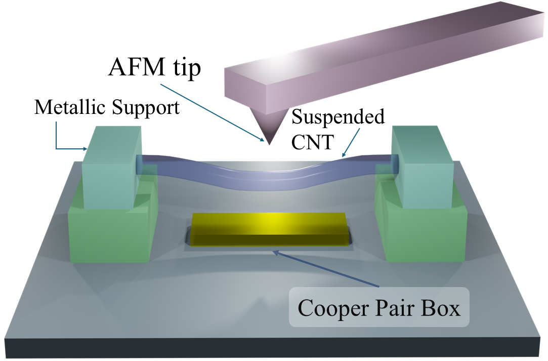
Figure 1: Schematic of the proposed experimental setup. A doubly clamped single-walled carbon nanotube (CNT) of length $L=100\text{--}1000\,\mathrm{nm}$ is suspended over a $200\,\mathrm{nm}$ trench and coherently driven by sub-femtonewton forces from a nearby atomic force microscope (AFM) tip. This experimental configuration provides a fully mechanical platform for implementing Ramsey interferometry and Wigner-function tomography of a nanomechanical mode under dilution-refrigerator conditions ($T=50\,\mathrm{mK}$, $P<10^{-7}\,\mathrm{Torr}$). Also indicated schematically is a Cooper-pair box patterned on the $\mathrm{SiO_{2}}/\mathrm{Si}$ substrate, illustrating one possible dispersive-coupling readout scheme for the CNT.

Environmental bath – The surrounding bosonic environment is modeled as a set of independent harmonic oscillators in thermal equilibrium, $H_{B}=\sum_{k}\hbar\omega_{k}b_{k}^{\dagger}b_{k}$. To lowest order, the CNT-environment coupling is described by the Hamiltonian [24]

$$H_{I}=\hbar\sigma_{z}\sum_{k}g_{k}\bigl(b_{k}^{\dagger}+b_{k}\bigr),$$ (2)

which induces both energy relaxation and dephasing. The coefficients $g_{k}$ in Eq. (2) represent coupling to bath mode $k$ with frequency $\omega_{k}$.

Combining the system, drive, and bath contributions, the laboratory‑frame Hamiltonian is:

$$H_{\text{lab}} =\frac{\hbar\omega_{0}}{2}\,\sigma_{z}+\hbar g\cos(\omega_{d}t)\,\sigma_{x}+\sum_{k}\hbar\omega_{k}b_{k}^{\dagger}b_{k}$$ (3)

$$\quad+\hbar\sigma_{z}\!\sum_{k}g_{k}\bigl(b_{k}^{\dagger}+b_{k}\bigr).$$

This expression represents the full Hamiltonian in the laboratory frame, containing a harmonically modulated $\sigma_{x}$ drive and longitudinal coupling to a bosonic bath.

System Hamiltonian in the rotating wave approximation. For weak driving, $g\ll\omega_{0}$ we transform the above Hamiltonian into a rotating frame and use the rotating wave approximation (RWA). First, introduce the unitary operator

$$U(t)=\exp\!\Bigl(i\frac{\omega_{d}t}{2}\sigma_{z}\Bigr),$$ (4)

which rotates the TLS about the $z$-axis at the drive frequency. Operators transform according to $\tilde{A}(t)=U(t)A\,U^{\dagger}(t)$ and by applying Eq. (4) to the free and drive Hamiltonians we get:

$$UH_{0}U^{\dagger} =\frac{\hbar}{2}(\omega_{0}-\omega_{d})\,\sigma_{z}\equiv\frac{\hbar\Delta}{2}\,\sigma_{z},$$ (5)

$$UH_{\mathrm{drv}}(t)U^{\dagger} =\hbar g\cos(\omega_{d}t)\Bigl[\sigma_{x}\cos(\omega_{d}t)+\sigma_{y}\sin(\omega_{d}t)\Bigr],$$ (6)

where $\Delta\equiv\omega_{0}-\omega_{d}$ is the detuning. Expanding the product of cosines/sines and applying the RWA we obtain the static contribution:

$$UH_{\mathrm{drv}}(t)U^{\dagger}\;\xrightarrow{\mathrm{RWA}}\;\frac{\hbar\Omega_{R}}{2}\,\sigma_{x},$$

with the Rabi frequency: $\Omega_{R}=g=F_{0}x_{\mathrm{zpf}}/{\hbar}$. Thus, the system Hamiltonian in the RWA approximation is:

$$H_{S}=\frac{\hbar\Delta}{2}\,\sigma_{z}+\frac{\hbar\Omega_{R}}{2}\,\sigma_{x}$$ (7)

Because $U(t)$ commutes with $H_{B}$ and $\sigma_{z}$, the environment Hamiltonian is unchanged: $\tilde{H}_{\mathrm{env}}=H_{B}+H_{I}$. Collecting all the terms we arrive at the rotating‑frame Hamiltonian:

$$\tilde{H}=\frac{\hbar\Delta}{2}\,\sigma_{z}+\frac{\hbar\Omega_{R}}{2}\,\sigma_{x}+\sum_{k}\hbar\omega_{k}b_{k}^{\dagger}b_{k}+\hbar\sigma_{z}\sum_{k}g_{k}\bigl(b_{k}^{\dagger}+b_{k}\bigr).$$ (8)

Physical picture – Because the AFM force couples linearly to the displacement operator, and only the co‑rotating component of the drive survives in the RWA, the AFM drive does work of order $F_{0}x_{\mathrm{zpf}}$ per cycle, setting a natural frequency scale. When the drive is on resonance ($\Delta=0$), the nanotube oscillates between $\ket{0}$ and $\ket{1}$ at the natural frequency scale given by the Rabi frequency $\Omega_{R}$. Off resonance ($\Delta\neq 0$) the oscillation frequency generalizes to $\Omega=\sqrt{\Delta^{2}+\Omega_{R}^{2}}$.

The bath coupling (last term in Eq. (8)) produces both energy relaxation and dephasing, which in the Born–Markov treatment leads to the Bloch relaxation and phase-coherence rates $\Gamma_{1}$ and $\Gamma_{2}$, discussed below. Eq. (8) is the starting point for analyzing Ramsey and Wigner‑tomography protocols for the mechanically driven CNT resonator.

III III. Lindblad Master Equation and Bloch Dynamics

Born-Markov approximation – The RWA Hamiltonian reads $\tilde{H}=H_{S}+H_{B}+H_{I}$ (Eq. (8)). In the interaction picture generated by $H_{S}+H_{B}$ the density matrix transforms as [24]: $\tilde{\rho}_{I}(t)=e^{i(H_{S}+H_{B})t/\hbar}\,\tilde{\rho}(t)\,e^{-i(H_{S}+H_{B})t/\hbar}$, and the interaction Hamiltonian becomes

$$H_{I}(t)=\hbar\sigma_{z}(t)\,\!B(t),\quad\begin{cases}\sigma_{z}(t)=e^{iH_{S}t/\hbar}\sigma_{z}e^{-iH_{S}t/\hbar},\\[4.0pt] B(t)=\displaystyle\sum_{k}g_{k}\bigl(b_{k}^{\dagger}e^{i\omega_{k}t}+b_{k}e^{-i\omega_{k}t}\bigr).\end{cases}$$ (9)

We make the following assumptions commonly employed in the theory of open quantum systems [24, 9]:

1. Born approximation: the composite state factorizes, $\tilde{\rho}_{I}(t)\approx\rho_{S}(t)\otimes\rho_{B}$, where $\rho_{B}=e^{-H_{B}/k_{B}T}/\Tr(e^{-H_{B}/k_{B}T})$ is stationary.

2. Markov approximation: bath correlations decay much faster than the timescale over which $\rho_{S}(t)$ changes appreciably.

3. RWA approximation: retain only terms oscillating slowly compared with the TLS transition frequencies.

These assumptions lead to the following time evolution equation for the reduced density matrix $\rho_{S}$ [24, 9]:

$$\dot{\rho}_{S}(t) =-\frac{1}{\hbar^{2}}\int_{0}^{\infty}\!d\tau\;\Tr_{B}\!\Bigl[\,H_{I}(t),\,\bigl[H_{I}(t-\tau),\,\rho_{S}(t)\otimes\rho_{B}\bigr]\Bigr].$$ (10)

Introducing the bath correlation function $C(\tau)=\langle B(\tau)B(0)\rangle_{B}$ and performing the $\tau$‐integral in Eq.  (10) one arrives at the standard Gorini–Kossakowski–Sudarshan–Lindblad (GKSL) equation [24, 9]:

$$\dot{\rho_{S}}=-\frac{i}{\hbar}[H_{S},\rho_{S}]+\gamma_{\downarrow}\,\mathcal{D}[\sigma_{-}]\rho_{S}+\gamma_{\uparrow}\,\mathcal{D}[\sigma_{+}]\rho_{S}+\gamma_{\varphi}\,\mathcal{D}[\sigma_{z}]\rho_{S},$$ (11)

with $\sigma_{+}=\ket{1}\!\bra{0}$, $\sigma_{-}=\ket{0}\!\bra{1}$, and the dissipator defined as:

$$\mathcal{D}[\sigma]\rho_{S}\equiv\sigma\rho_{S}\sigma^{\dagger}-\tfrac{1}{2}\{\sigma^{\dagger}\sigma,\rho_{S}\}.$$ (12)

Here $\gamma_{\downarrow}$ ($\gamma_{\uparrow}$) is the relaxation (thermal excitation) rate set by the bath spectral density at $\omega_{0}$, and $\gamma_{\varphi}$ accounts for pure dephasing, typically dominated by low-frequency phase noise.

Physical picture – Starting from the Hamiltonian in Eq. (8), the Born–Markov approximation yields the GKSL master equation (Eq. (11)). The system Hamiltonian $H_{S}$ (Eq. (7)) describes the unitary evolution for the driven CNT resonator. The commutator $-i[H_{S},\rho_{S}]/\hbar$ is the familiar Liouville–von Neumann term $\partial_{t}\rho_{S}=-i[H_{S},\rho_{S}]/\hbar$ for an isolated quantum system. Coherent excitation by the AFM drive is included in $H_{S}$. Each additional term in Eq. (11) has the structure $\gamma_{j}\,\mathcal{D}[\sigma_{j}]\rho_{S}$ with the dissipator $\mathcal{D}[\sigma]\rho_{S}$ defined in Eq. (12). The dissipator generates irreversible, stochastic jumps associated with processes in the environment. The operators $\sigma\in\{\sigma_{-},\,\sigma_{+},\,\sigma_{z}\}$ serve as Lindblad jump operators, and capture specific physical processes (incoherent population jumps, dephasing) induced by the environment:

$\bullet$ $\sigma_{-}$ ($=\ket{0}\!\bra{1}$) : energy relaxation ($\ket{1}\to\ket{0}$).

$\bullet$ $\sigma_{+}$ ($=\ket{1}\!\bra{0}$) : incoherent excitation ($\ket{0}\to\ket{1}$).

$\bullet$ $\sigma_{z}$ : pure dephasing that leaves populations unchanged.

The gain term $\sigma\rho_{S}\sigma^{\dagger}$ in Eq. (12) adds population or coherence consistent with the jump. The loss term $-\tfrac{1}{2}\{\sigma^{\dagger}\sigma,\rho_{S}\}$ subtracts terms such that the total evolution preserves $\Tr\rho_{S}=1$. This competition between coherent drive and dissipative processes sets the visibility of Rabi oscillations, Ramsey fringes, and the regions where the Wigner function is negative for the CNT oscillator.

The resulting rates describe incoherent (e.g. thermal) excitation ($\gamma_{\uparrow}$), relaxation ($\gamma_{\downarrow}$), and slow longitudinal frequency noise ($\gamma_{\varphi}$), thereby establishing a quantitative connection between the microscopic properties of the environment and the observable relaxation and dephasing times for the mechanically driven CNT resonator. These dissipative rates have dimensions of inverse time, and are set by the bath spectral density and temperature. For a transition at frequency $\omega_{0}$ [24, 9]:

$$\gamma_{\uparrow}=2\pi J(\omega_{0})\,n(\omega_{0}),\qquad\gamma_{\downarrow}=2\pi J(\omega_{0})\,[n(\omega_{0})+1]$$ (13)

where $J(\omega)=2\alpha\,\omega\,e^{-\omega/\omega_{c}}$ is the Ohmic spectral density (with dimensionless coupling $\alpha$ and cutoff $\omega_{c}$), and $n(\omega)=\bigl[e^{\hbar\omega/k_{B}T}-1\bigr]^{-1}$ is the thermal occupation number.

Bloch dynamics for the AFM-driven CNT under dissipation – The Bloch decay parameters and the corresponding time constants are defined as:

$$T_{1}\equiv\frac{1}{\Gamma_{1}},\qquad T_{2}\equiv\frac{1}{\Gamma_{2}},\qquad\Gamma_{1}\equiv\gamma_{\downarrow}+\gamma_{\uparrow},\quad\Gamma_{2}\equiv\frac{\Gamma_{1}}{2}+2\gamma_{\varphi},$$ (14)

The corresponding time constants quantify longitudinal energy relaxation ($T_{1}$) and transverse phase coherence ($T_{2}$) [9, 24].

A pure-dephasing rate arises from slow longitudinal frequency noise and, for an Ohmic bath, scales as $\gamma_{\varphi}\;\simeq\;2\pi\alpha\,k_{B}T/\hbar$ [24, 9]. Therefore, in the relaxation-limited regime (i.e., when slow longitudinal fluctuations are negligible on the experimental timescale), we have $\gamma_{\varphi}\approx 0$ and thus $\Gamma_{2}=\Gamma_{1}/2$.

By introducing the Bloch vector components:

$$\,X\equiv\Tr(\sigma_{x}\rho_{S}),\qquad Y\equiv\Tr(\sigma_{y}\rho_{S}),\qquad Z\equiv\Tr(\sigma_{z}\rho_{S})\,$$ (15)

the expression for the reduced density matrix becomes [24]:

$$\rho_{S}=\tfrac{1}{2}\bigl(\openone+X\sigma_{x}+Y\sigma_{y}+Z\sigma_{z}\bigr).$$ (16)

We substitute the Bloch representation (Eq. (16)) into the GKSL equation (Eq. (11)) and explicitly evaluate each term in the dissipator (Eq. (12)) using the commutation relations $[\,\sigma_{i},\sigma_{j}\,]=2i\varepsilon_{ijk}\sigma_{k}$. Straightforward algebra yields the Bloch equations for a mechanically driven CNT coupled to its environment:

$$\dot{X} =-\Gamma_{2}X+\Delta Y,$$ (17)

$$\dot{Y} =-\Gamma_{2}Y-\Delta X+\Omega_{R}Z,$$ (18)

$$\dot{Z} =-\Gamma_{1}(Z-Z_{\!\mathrm{eq}})-\Omega_{R}Y,$$ (19)

with the thermal inversion $Z_{\!\mathrm{eq}}=(\gamma_{\uparrow}-\gamma_{\downarrow})/(\gamma_{\uparrow}+\gamma_{\downarrow})=-\tanh\!\bigl(\hbar\omega_{0}/2k_{B}T\bigr)$ [24]. For an Ohmic spectral density at dilution temperatures we obtain $Z_{\!\mathrm{eq}}\approx-1$.

Physical picture – The longitudinal relaxation time $T_{1}$ characterizes population relaxation towards thermal equilibrium, energy decay from $\ket{1}$ to $\ket{0}$ and thermal repopulation. Physically, $T_{1}$ quantifies how rapidly an excited nanotube state $\ket{1}$ decays to $\ket{0}$ (via $\gamma_{\downarrow}$) while the thermal bath repopulates $\ket{1}$ with rate $\gamma_{\uparrow}$. The phase‑coherence time $T_{2}$, governs the exponential decay of the off‑diagonal density‑matrix elements. In the relaxation-limited regime $\gamma_{\varphi}\approx 0$, and $T_{2}\simeq 2T_{1}$

Eqs. (14)–(19) clarify the relevant control and decay scales: the oscillator frequency $\omega_{0}$ defines the intrinsic timescale, the Rabi frequency $\Omega_{R}$ controls the coherent rotation rate induced by AFM driving, and the detuning $\Delta$ determines the Bloch vector precession during free evolution (Ramsey phase accumulation). The transverse coherence time $T_{2}$ fixes the fringe contrast, while the longitudinal relaxation time $T_{1}$ governs the free decay of the population (”ringdown”) once the drive is switched off. Under continuous resonant drive, the steady state reflects competition between the drive strength and two relaxation channels: energy exchange with the bath ($T_{1}$) and loss of phase coherence ($T_{2}$). Operationally, $T_{1}$ sets the rate of energy dissipation/repopulation, whereas $T_{2}$ determines how long the relative phase between $\ket{0}$ and $\ket{1}$ is maintained, thereby controlling the visibility of Ramsey fringes and limiting the spectroscopic linewidth.

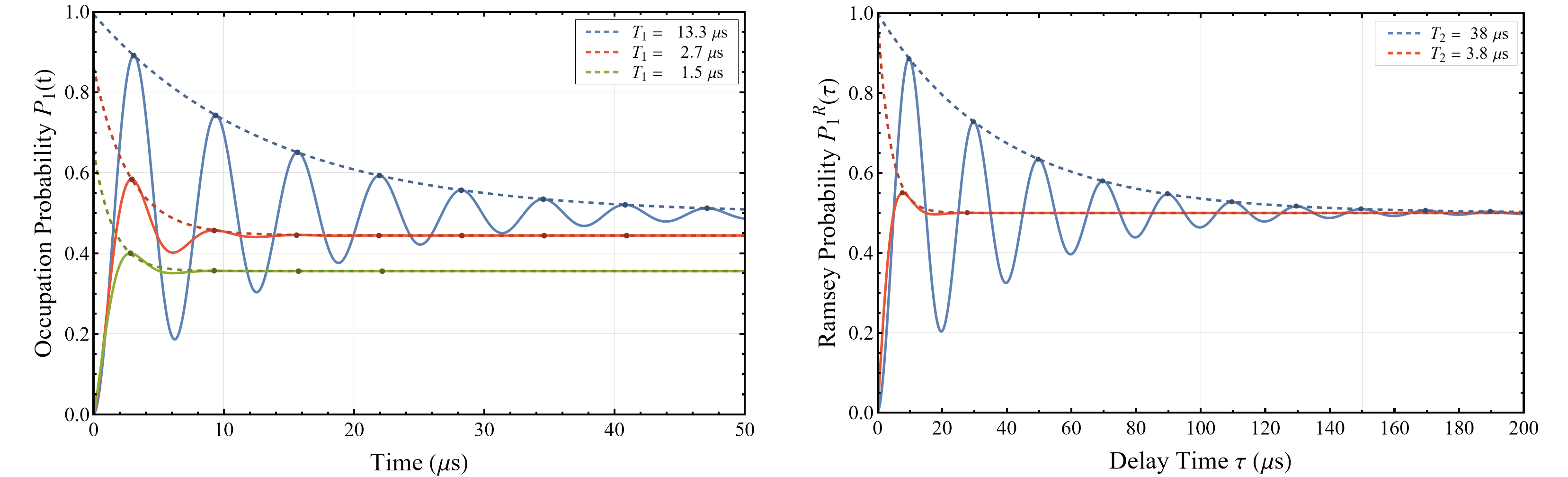
(a) (b)

Figure 2: (a) Excited-state population $P_{1}(t)$ of a driven CNT in three damping regimes: strong driving ($\Gamma_{1}/\Omega_{R}=0.1$, blue), underdamped ($\Gamma_{1}/\Omega_{R}=0.5$, red), and near-critical ($\Gamma_{1}/\Omega_{R}=0.9$, green). The Rabi frequency is $\Omega_{R}=$0.75\text{\,}\mathrm{M}\mathrm{H}\mathrm{z}$$ for all curves. Dotted lines are fits to Eq. (24) used to extract $T_{1}$. (b) Ramsey population $P_{1}^{\mathrm{R}}(\tau)$ versus delay for detuning $\Delta=$300\text{\,}\mathrm{k}\mathrm{H}\mathrm{z}$$ in two CNT devices of different lengths: $L=$800\text{\,}\mathrm{nm}$$ (blue) and $L=$250\text{\,}\mathrm{nm}$$ (red). Dotted lines are fits to Eq. (29) used to extract $T_{2}$.

IV IV. Rabi Oscillations and Ramsey Interferometry

We show that on resonance ($\Delta=0$), at dilution temperatures ($\sim 50$ mK), and with the system initialized in the ground state $\ket{0}$, the mechanically driven CNT undergoes damped Rabi oscillations. By choosing zero detuning $\Delta=\omega_{0}-\omega_{d}=0$ and shift $z(t)=Z(t)-Z_{\!\mathrm{eq}}$, the Bloch equations (17)–(19) become:

$$\dot{X}=-\Gamma_{2}\,X,\;\dot{Y}=-\Gamma_{2}\,Y+\Omega_{R}(z+Z_{\!\mathrm{eq}}),\;\dot{z}=-\Gamma_{1}\,z-\Omega_{R}\,Y$$

which are homogeneous in $(Y,z)$ apart from the constant term $\Omega_{R}Z_{\!\mathrm{eq}}$. After eliminating $X$ and $Y$, the shifted $z$–component satisfies the following equation:

$$\ddot{z}+2\lambda\dot{z}+(\lambda^{2}+\Omega_{d}^{2})z=-\,\Omega_{R}^{2}Z_{\text{eq}},$$ (20)

with $\lambda=({\Gamma_{1}+\Gamma_{2}})/{2}$ and the damped frequency $\Omega_{d}\equiv\ \sqrt{\Omega_{R}^{2}-(\Gamma_{1}-\Gamma_{2})^{2}/4}$. The physical $Z$–Bloch component is:

$$Z(t)=z(t)+Z_{\text{eq}}.$$ (21)

Once $Z(t)$ is known, the probability of occupying the first excited vibrational state $\ket{1}$ is given by [24]:

$$\;P_{1}(t)=\frac{1+Z(t)}{2}\;,$$ (22)

We assume the CNT is initially in the ground state $\{\ket{0}\}$, so the Bloch vector starts at the south pole:

$$Z(0)=-1\;\Longrightarrow\;z(0)=-1-Z_{\text{eq}},\ \dot{z}(0)=\Gamma_{1}(1+Z_{\text{eq}}).$$ (23)

Moreover, we assume that the system is at cryogenic temperatures ($\sim 50$mK) such that the thermal inversion $Z_{\!\mathrm{eq}}\approx-1$, as discussed in the previous section. Solving Eq. (20) with these conditions, and using Eq. (22) we obtain the following expression for the excited-state occupation probability:

$$P_{1}(t) =\frac{\Omega_{R}^{2}}{2\big(\Omega_{R}^{2}+\Gamma_{1}\Gamma_{2}\big)}\cdot$$ (24)

$$\cdot\Big[1-e^{-(\Gamma_{1}+\Gamma_{2})t/2}\Big(\cos(\Omega_{d}t)+\frac{\Gamma_{1}-\Gamma_{2}}{2\,\Omega_{d}}\sin(\Omega_{d}t)\Big)\Big],$$

with the on-resonance steady state

$$P_{1}^{(\infty)}=\Omega_{R}^{2}/{\big(2\Omega_{R}^{2}+2\Gamma_{1}\Gamma_{2}\big)}.$$

In the relaxation-limited regime with negligible pure dephasing ($\gamma_{\varphi}\!\approx\!0$), one has $\Gamma_{2}\!\approx\!\Gamma_{1}/2$, and the Rabi oscillation envelope decays at rate $3\Gamma_{1}/4$. Additional pure dephasing increases $\Gamma_{2}$ while leaving $\Gamma_{1}$ unchanged, thereby reducing the oscillation visibility and shrinking the underdamped window $\Omega_{R}>\tfrac{1}{2}|\Gamma_{1}-\Gamma_{2}|$. The free population ringdown time remains set by $T_{1}$. Fig. 2(a) displays the time evolution of the excited-state occupation probability for different values of the oscillation parameters.

Ramsey Interferometry – provides a phase-sensitive probe of coherence complementary to the driven dynamics of Rabi oscillations. In the present scheme a calibrated AFM tip generates two mechanical $\pi/2$ pulses separated by a free-evolution interval $\tau$. The pulse sequence is:

$$\ket{0}\xrightarrow{\pi/2}\frac{\ket{0}+\ket{1}}{\sqrt{2}}\xrightarrow{\text{free }\tau}\rho(\tau)\xrightarrow{\pi/2}\rho_{\mathrm{out}}(\tau)\xrightarrow{\text{readout}}P_{1}^{R}(\tau).$$

The first pulse creates a $\pi/2$ rotation for a short resonant drive $t_{\pi/2}=\pi/(2\Omega_{R})$, and prepares the CNT in a coherent superposition $\ket{\psi(0)}=(\ket{0}+\ket{1})/\sqrt{2}$. We choose the phase of the first resonant $\pi/2$ pulse such that the Bloch vector becomes: $(1,0,0)$. During the subsequent delay interval $\tau$ the Bloch vector precesses at the detuning frequency $\Delta$, and the system acquires a relative phase $\Delta\tau$ induced by the unitary evolution. Since during this free interval the drive is off, $\Omega_{R}(t)=0$, and the Bloch equations (17)–(19) decouple. With initial condition $(X,Y)=(1,0)$ at $t=0$ one obtains:

$$X(\tau) =e^{-\tau/T_{2}}\cos(\Delta\tau),$$ (25)

$$Y(\tau) =e^{-\tau/T_{2}}\sin(\Delta\tau),$$ (26)

independent of $T_{1}$. The longitudinal component $Z(\tau)$ does not enter the ideal Ramsey signal below.

The second $\pi/2$ pulse converts the accumulated phase into a population difference. Let this pulse have phase $\phi_{0}$ (set by the programmed phase between the two AFM pulses). A $\pi/2$ rotation about an equatorial axis with azimuth $\phi_{0}$ maps the equatorial projection $(X,Y)$ onto the $Z$ axis according to

$$Z_{\mathrm{f}}=X(\tau)\cos\phi_{0}+Y(\tau)\sin\phi_{0},$$ (27)

and the excited-state probability after the second pulse is

$$P_{1}^{\mathrm{R}}(\tau)=\frac{1+Z_{\mathrm{f}}}{2}.$$ (28)

Substituting Eqs. (25)–(26) into Eq. (27) and then into Eq. (28) yields the Ramsey excited-state probability:

$$P_{1}^{\mathrm{R}}(\tau)=\tfrac{1}{2}\Big[1+e^{-\tau/T_{2}}\cos(\Delta\tau+\phi_{0})\Big],$$ (29)

where $\phi_{0}$ captures any programmed phase shift between AFM pulses. In our protocol $P_{1}^{\mathrm{R}}(\tau)$ is measured immediately after the second pulse, using any of the compatible transducers described below (AFM deflection, dispersive Cooper-pair box, or cavity reflectometry). Sweeping $\tau$ produces Ramsey fringes whose frequency is set by the detuning $\Delta$ and whose envelope decays with $T_{2}$. We operate with $\Omega_{R},\Delta\ll\omega_{0}$ (RWA regime) and use short pulses, $t_{\pi/2}\ll\tau,T_{2}$, so decoherence during the pulses is negligible. The relative phase $\phi_{0}$ is set by timing the second pulse with respect to the drive. On resonance ($\Delta=0$) this enables phase scans at fixed $\tau$. Projective measurements in the $\left\{\ket{0},\ket{1}\right\}$ basis then return $P_{1}^{\mathrm{R}}(\tau)$ with explicit dependence on the accumulated phase $\Delta\tau$ or the programmed phase $\phi_{0}$ (Eq. (29)). Fig. 2(b) shows the plot of the Ramsey probability as a function of the delay time for different drive and dephasing parameters. The $\tau$-dependent modulation of the measurement statistics provides direct evidence of a coherent superposition of the two levels. The energy-relaxation time $T_{1}$ can be obtained independently from the ringdown, $T_{1}=Q/\omega_{0}$, where $Q$ is the CNT mechanical quality factor [18]. This all-mechanical implementation eliminates on-chip microwave drive lines at the resonator, avoids optical heating, and uses the same actuator to deliver phase-space displacements for Wigner tomography, thereby unifying control and state reconstruction in a single device, as we show in the next section.

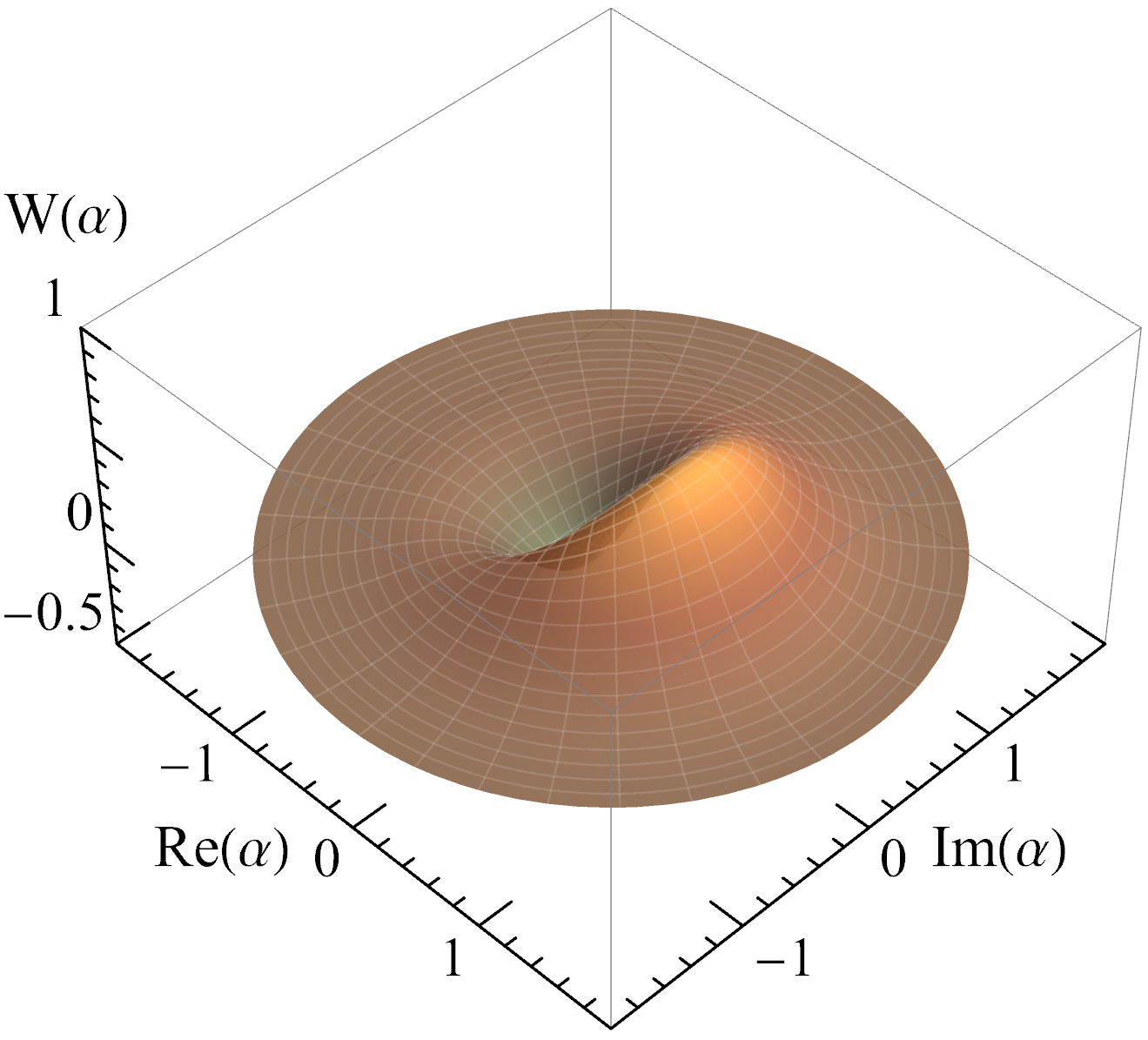
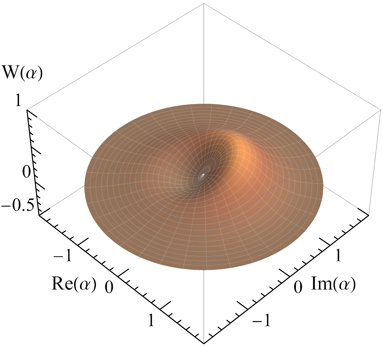
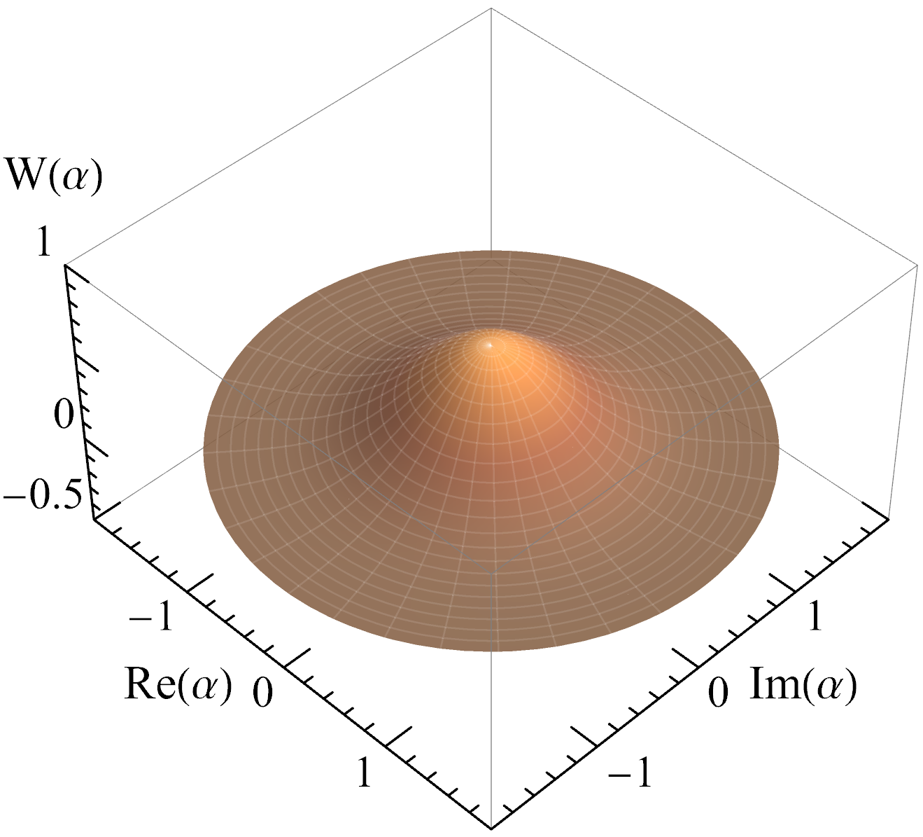
(a)   (b) (c)

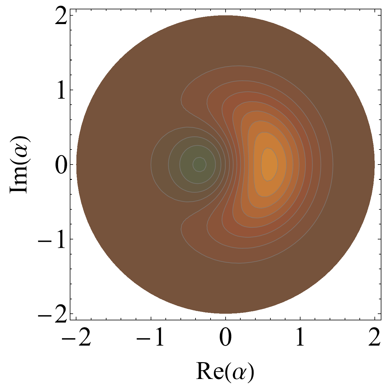
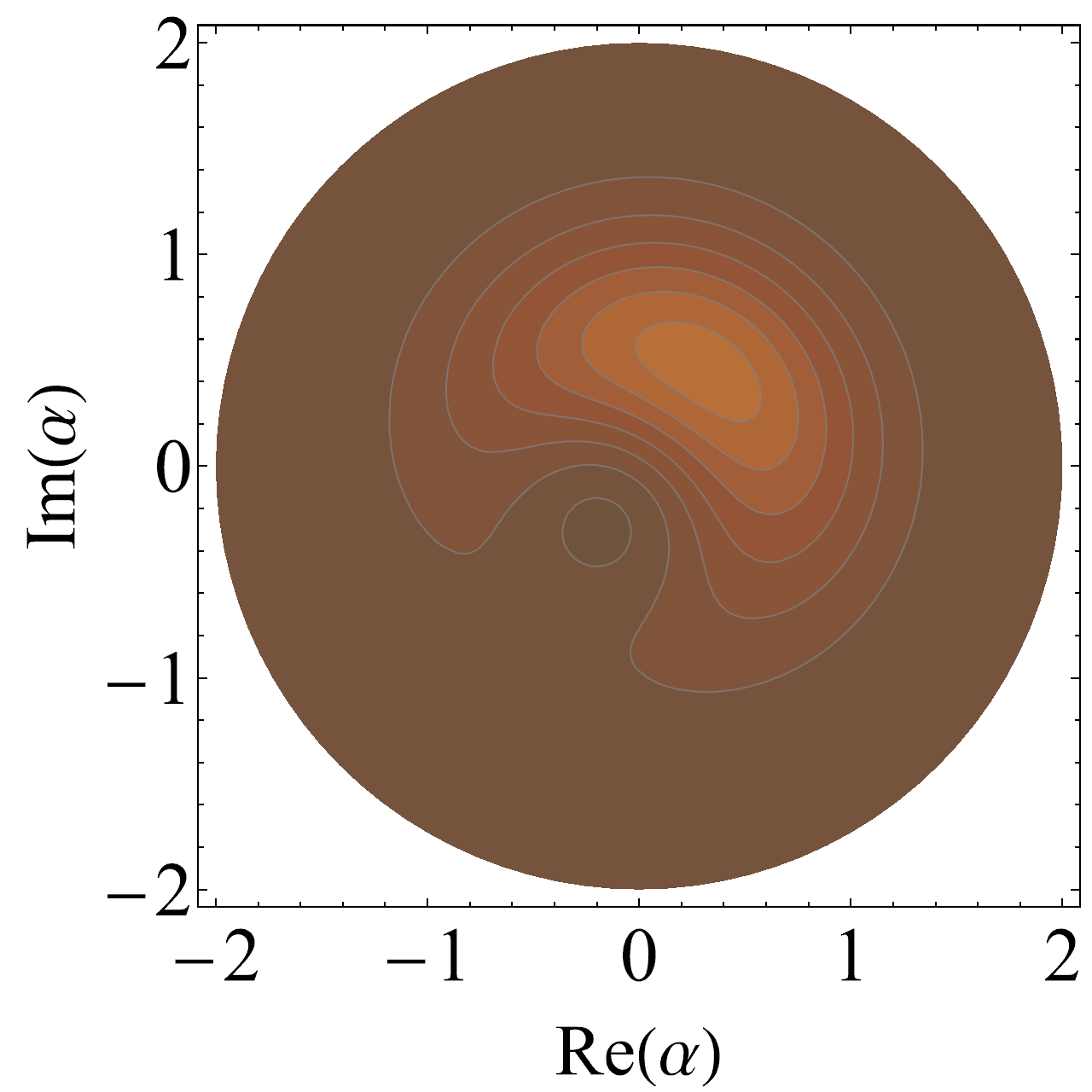
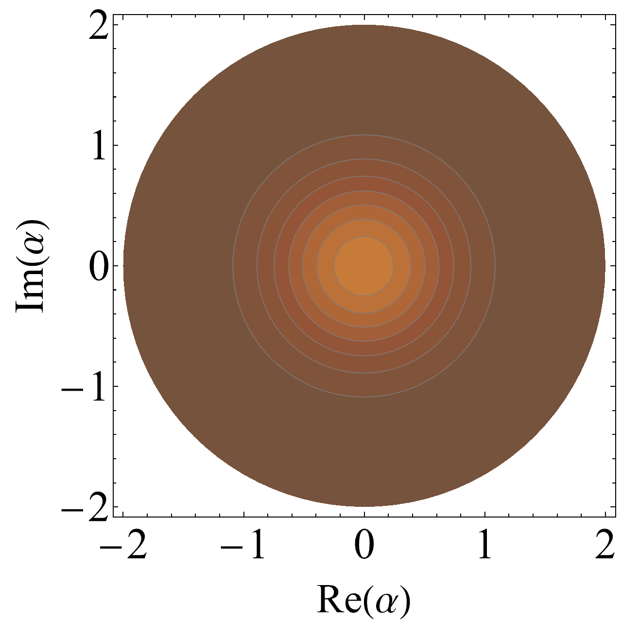
(d)    (e) (f)

Figure 3: Time evolution of the calculated Wigner function $W(\alpha)$. For all panels, $T_{1}=5/\omega_{0}$. Top row: 3D surfaces showing $W(\alpha)$ at $t=0$ (a), $t=T_{1}$ (b), and $t=5T_{1}$ (c). Bottom row: corresponding 2D plots at $t=0$ (d), $t=T_{1}$ (e), and $t=5T_{1}$ (f). A single color scale is shown on the right, applying to all six panels.

V V. Wigner Tomography

The Wigner function $W$ provides a complete quasi-probability description of the CNT flexural mode in phase space, formally equivalent to the density matrix description [25, 26]. Because it is not a true probability distribution, $W$ can take on negative values, which provide clear signatures of nonclassicality and quantum interference, and this makes it especially useful for visualizing and tracking decoherence. Experimentally, $W$ can be reconstructed (“Wigner tomography”) from repeated measurements on identically prepared states by recording projections along rotated or skewed phase-space axes and inverting them (for example, via an inverse Radon transform), or, equivalently by measuring displaced parity. These approaches are well established in platforms such as matter-wave interferometry and trapped-ion motion [21, 8, 27, 28, 29, 30, 25].

We now calculate the Wigner function explicitly for the CNT flexural mode. As established in the previous section, immediately after preparation the CNT is in the coherent superposition $\ket{\psi(0)}=(\ket{0}+\ket{1})/\sqrt{2}$ with density matrix

$$\rho_{S}(0)=\frac{1}{2}\begin{pmatrix}1&1\\[2.0pt] 1&1\end{pmatrix}$$

Coupling to a bath produces longitudinal relaxation at rate $\Gamma_{1}=1/T_{1}$ and transverse decay at rate $\Gamma_{2}=1/T_{2}$. Within the Born–Markov approximation, and in the relaxation-limited regime (negligible pure dephasing, such that $T_{2}\simeq 2T_{1}$) and cold-bath limit ($n_{\mathrm{th}}\!\ll\!1$), the density-matrix elements evolve as [24]:

$$\rho_{11}(t) =\rho_{11}(0)\,e^{-\Gamma_{1}t},\quad\rho_{00}(t)=1-\rho_{11}(t),$$ (30)

$$\rho_{01}(t) =\rho_{01}(0)\,e^{-(\Gamma_{1}/2+i\omega_{0})t},\quad\rho_{10}(t)=\rho_{01}^{\ast}(t).$$

The Wigner function associated with $\rho_{S}$ is [24]:

$$W(\alpha)=\frac{2}{\pi}\,e^{-2|\alpha|^{2}}\Bigl[\rho_{00}+\rho_{11}\bigl(4|\alpha|^{2}-1\bigr)+2\,\real\!\bigl(2\alpha\,\rho_{10}\bigr)\Bigr],$$ (31)

where $\alpha=(X+iP)/\sqrt{2}$ is the phase-space coordinate. Writing $\alpha=r\,e^{i\theta}$ with $r\geq 0$, and inserting Eq. (30) yields the time-dependent Wigner function

$$W(r,\theta;t) =\frac{2}{\pi}\,e^{-2r^{2}}\Bigl[(1-P(t))+P(t)\,(4r^{2}-1)$$ (32)

$$\quad+2r\,e^{-t/T_{2}}\cos\!\bigl(\theta-\omega_{0}t\bigr)\Bigr],$$

with $P(t)=\rho_{11}(t)=\tfrac{1}{2}\,e^{-t/T_{1}}$.

Fig. 3 shows the time evolution of the calculated $W(\alpha)$ for the CNT. Regions with $W(\alpha)<0$ are a hallmark of nonclassicality arising from interference between coherently superposed vibrational states and are clearly visible at early times (panels (a), (b), (d), (e)). As the CNT mode evolves under environmental decoherence (energy relaxation and dephasing), these interference features are progressively washed out, and $W(\alpha)$ approaches a positive, broadened Wigner distribution that tends to the ground state Gaussian at long times (panels (c) and (f)). In the limiting cases:

• Initial state $(t=0)$: $P(0)=\tfrac{1}{2}$$e^{-t/T_{1}}=1/2$,

  $$W(r,\theta;0)=\frac{2}{\pi}e^{-2r^{2}}\Bigl[\,2r^{2}+2r\cos\theta\Bigr],$$ (33)

  showing a negative lobe near the origin (quantum-interference signature).

• Intermediate times ($t\sim T_{1}$): the coherence term decays as $e^{-t/T_{2}}$, and the state approaches a positive mixture of $\ket{0}$ and $\ket{1}$.

• Long times $(t\gg T_{1})$: $P(t)\to 0$ and $e^{-t/T_{2}}\to 0$, so $W\approx\dfrac{2}{\pi}e^{-2r^{2}},$ the Gaussian Wigner function of the ground state $\ket{0}$.

Building on these results, we propose a measurement scheme that applies a short, near-resonant AFM impulse to implement the phase-space displacement

$$D(\alpha)=\exp(\alpha a^{\dagger}-\alpha^{*}a),\qquad\alpha=\frac{F_{0}t_{d}}{\sqrt{2m_{\!\mathrm{eff}}\hbar\omega_{0}}}\,e^{i\phi_{d}},$$ (34)

where $F_{0}$ and $t_{d}$ are the pulse amplitude and duration, $\phi_{d}$ is the phase of the AFM drive relative to the oscillator, and $m_{\!\mathrm{eff}},\,\omega_{0}$ are the effective mass and frequency of the CNT fundamental flexural mode. After the calibrated displacement, measuring the parity operator $\hat{\Pi}=e^{i\pi a^{\dagger}a}=(-1)^{\hat{n}}$ yields the displaced-parity form of the Wigner function [28, 27, 29]:

$$W(\alpha)=\frac{2}{\pi}\mathrm{Tr}\big[D(-\alpha)\,\rho_{S}\,D(\alpha)\,\hat{\Pi}\big]\quad.$$ (35)

Thus, the same AFM actuator that generates $\pi/2$ rotations (Rabi/Ramsey calibration) also provides the controlled phase-space displacements $D(\alpha)$ required for Wigner tomography. Parity is converted to a measured excited state population by a Ramsey-type sequence $\{\pi/2,\ t_{\pi},\ -\pi/2\}$ that accumulates a number-dependent phase $\chi\hat{n}t_{\pi}$. Here, $-\pi/2$ denotes a $\pi/2$ pulse with a $\pi$-phase flip of the drive. Choosing $t_{\pi}=\pi/\chi$ implements the parity phase $e^{i\pi\hat{n}}$. The parameter $\chi$ is the effective parity-mapping rate per phonon set by the CPB-CNT or cavity-CNT dispersive coupling (details in the next section). This yields the excited–state probability [28, 27, 29]:

$$P_{1}(\alpha)=\tfrac{1}{2}\big[1-\frac{\pi}{2}W(\alpha)\big],\qquad 2\pi/\omega_{0}\ll t_{\pi}\ll T_{2}.$$ (36)

Sweeping $\alpha$ on a grid maps $W(\alpha)$ directly via displaced-parity measurements, without any inverse transform or numerical reconstruction. The contrast across the map is limited by $T_{2}$ during the parity mapping window $t_{\pi}$ and by any displacement-induced dephasing.

VI VI. Readout modalities

We propose four different readout schemes: AFM deflection, Dispersive CPB, Dispersive cavity, and Direct mechanics cavity. All four methods share the same all-mechanical basic controls (AFM $\pi/2$ rotations and displacements), extending the Ramsey interferometer into a full, state-resolved characterization of the phase space.

VI.1 A. AFM deflection and direct population readout

Immediately after the Ramsey sequence, the CNT displacement is transduced by the AFM probe (optical/electrical deflection or weak probe force) described by

$$H_{\rm meas}(t)=-F_{\rm probe}(t)\,x=-F_{\rm probe}(t)\,x_{\!{\rm zpf}}(a+a^{\dagger}).$$ (37)

Linear demodulation of the deflection quadrature distinguishes $\ket{1}$ from $\ket{0}$, returning $P_{1}$ in a single readout. The mechanical ringdown of the demodulated signal yields the longitudinal relaxation time $T_{1}$, while sweeping the Ramsey delay $\tau$ gives the detuning frequency $\Delta$ and phase coherence time $T_{2}$. This channel is used to measure population and characterize decoherence. Practical implementation follows the Ramsey calibration: (i) set $\omega_{d}\approx\omega_{0}$ and determine $\Omega_{R}$ via a Rabi scan; (ii) choose $t_{\pi/2}=\pi/(2\Omega_{R})$, (iii) synchronize two identical $\pi/2$ pulses with programmable delay $\tau$, and (iv) demodulate the AFM signal during a short integration window after the second pulse. Typical operating times are $t_{\pi/2}\sim 0.1$–$0.3\,\mu$s, $\tau=0.1$–$50\,\mu$s. Readout is performed via lock-in or IQ demodulation referenced to the drive frequency $\omega_{d}$.

VI.2 B. Dispersive CPB readout and parity mapping

A Cooper–pair box dispersively coupled to the CNT implements a phase proportional to the phonon-number operator $\hat{n}=a^{\dagger}a$ during the Ramsey free-evolution window [1, 4]. The Jaynes–Cummings interaction is

$$\frac{H}{\hbar}=\omega_{0}\,a^{\dagger}a+\frac{\omega_{q}}{2}\sigma_{z}+g_{m}\big(a\sigma_{+}+a^{\dagger}\sigma_{-}\big),$$ (38)

where $\omega_{0}$ is the CNT flexural-mode frequency, $\omega_{q}$ is the CPB qubit transition frequency, and $g_{m}$ is the CPB–CNT coupling. The CPB–CNT mechanical-mode detuning is $\Delta_{q}\equiv\omega_{q}-\omega_{0}$. For $|\Delta_{q}|\gg g_{m}$, the interaction reduces to the dispersive Hamiltonian [31, 32, 33, 34]:

$$\frac{H_{\rm int}^{(\rm CPB)}}{\hbar}\simeq\chi\,a^{\dagger}a\,\frac{\sigma_{z}}{2},\qquad\chi\simeq\frac{2g_{m}^{2}}{\Delta_{q}}\ .$$ (39)

Mechanical implementations of such dispersive couplings have been demonstrated with CPB/transmon devices [35, 36, 2]. During a calibrated window $t_{\pi}=\pi/\chi$, the CPB acquires the number-dependent phase $\chi t_{\pi}\,\hat{n}$, implementing $e^{i\pi\hat{n}}$. When the Ramsey sequence is preceded by a mechanical displacement $D(\alpha)$ and performed with the pulse sequence $\{\pi/2,\,t_{\pi},\,-\pi/2\}$ (where $-\pi/2$ denotes a $\pi/2$ rotation with a $\pi$-phase flip of the drive), the excited-state probability encodes the displaced parity signal as given in Eq. (36). High-contrast mapping requires $2\pi/\omega_{0}\ll t_{\pi}\ll T_{2}$, and dephasing during $t_{\pi}$ limits the contrast.

In a purely mechanical variant, a weak Duffing (self-Kerr) term arising from tension-induced geometric effects and/or electrostatic forces [31, 32, 33, 34, 37] yields an effective number-dependent phase rate $\chi$ and realizes the same parity gate $e^{i\pi\hat{n}}$, with $t_{\pi}=\pi/\chi$. For typical CNT resonators $(L\sim 0.1\text{–}1~\mu\mathrm{m})$, this corresponds to $t_{\pi}\sim 1\text{–}20~\mu\mathrm{s}$.

VI.3 C. Dispersive cavity readout

A microwave cavity operated in the dispersive regime provides phase-sensitive readout of the CPB qubit state during the Ramsey sequence. The effective readout Hamiltonian is

$$\frac{H_{\rm read}}{\hbar}=\omega_{c}\,a_{c}^{\dagger}a_{c}+\frac{\tilde{\omega}_{q}}{2}\,\sigma_{z}+\chi_{c}\,a_{c}^{\dagger}a_{c}\,\frac{\sigma_{z}}{2}.$$ (40)

Here, $\omega_{c}$ is the bare cavity angular frequency; $a_{c}$ ($a_{c}^{\dagger}$) annihilates (creates) a cavity photon; $\tilde{\omega}_{q}$ is the dressed CPB qubit transition frequency (including static Lamb/AC-Stark shifts); and $\chi_{c}$ is the dispersive coupling (“cavity pull”) that produces a CPB state–dependent cavity shift $\omega_{c}\!\to\!\omega_{c}\pm\chi_{c}/2$ for $\sigma_{z}=\pm 1$ [31, 32, 33, 34].

Homodyne detection – The cavity is driven near $\omega_{c}$ and the transmitted (or reflected) field is routed through cryogenic circulators/isolators and a high electron mobility transistor (HEMT) low-noise amplifier [38, 39]. The signal is mixed with a local oscillator (LO) phase-locked to the cavity probe in an IQ mixer to yield baseband voltages $I(t)$ and $Q(t)$. The instantaneous phase $\phi(t)=\arctan[Q(t)/I(t)]$ (or an appropriate quadrature) tracks the CPB qubit observable $\sigma_{z}$, since the CPB state–dependent pull $\pm\chi_{c}/2$ rotates the cavity response in the complex plane [38, 39]. Integration over a window set by the cavity linewidth provides the Ramsey or parity-mapped population used in the analysis.

VI.4 D. Direct mechanics cavity readout

As an alternative to CPB-based readout, one may couple the cavity directly to the CNT mode to produce either a cross-Kerr interaction [40]:

$$\frac{H_{\rm int}^{(\rm mc)}}{\hbar}\simeq\chi_{mc}\,a^{\dagger}a\,a_{c}^{\dagger}a_{c},$$ (41)

or a radiation-pressure interaction [32, 40]:

$$\frac{H_{\rm rp}}{\hbar}=-g_{0}\,a_{c}^{\dagger}a_{c}\,(a+a^{\dagger}),$$ (42)

where $a,a^{\dagger}$ denote the CNT mechanical modes and $a_{c}$, $a_{c}^{\dagger}$ the cavity modes. During the Ramsey free-evolution window, these couplings generate an effective phase rate $\chi_{\rm eff}$ proportional to the CNT phonon number $\hat{n}$, so the same parity gate $e^{i\pi\hat{n}}$ is realized by choosing $t_{\pi}=\pi/\chi_{\rm eff}$. The tomography framework and normalization are the same as described above.

VI.5 E. Practical timing, calibration, and acquisition

Mechanical rotations are kept short $(t_{\pi/2}\!\ll\!\tau,\,T_{2})$ to minimize pulse-induced dephasing. The relative phase of the second $\pi/2$ rotation is set either by a $\pi$ phase flip of the drive or by a half-period timing slip $t=\pi/\omega_{d}$. The parity-mapping window $t_{\pi}$ is chosen using an estimate of $\chi$ and then fine-tuned by maximizing contrast, subject to the condition $2\pi/\omega_{0}\ll t_{\pi}\ll T_{2}$ (see part (b) above). The Ramsey population $P_{1}^{R}(\tau)$ is fitted to the expressions given in Eq. (29).

Calibration follows the sequence summarized in (a): Rabi scans set $\Omega_{R}$ and $t_{\pi/2}$, Ramsey scans determine $\Delta$ and $T_{2}$, and mechanical ringdown yields $T_{1}$. The displacement for $D(\alpha)$ is obtained from the small-signal transfer function. The waveform generator, digitizer, and LO share a common frequency reference. Hardware gating minimizes relative jitter and slow LO-phase drift is tracked with interleaved references [38, 39].

For cavity readout, the I/Q record (part (c) above) is integrated with a matched filter over a window on the order of the cavity photon lifetime, chosen to remain well within the CPB $T_{1}$. For AFM deflection readout, the demodulated quadrature at $\omega_{d}$ is integrated over a short $\mu$s-scale window placed after the second pulse to avoid drive transients, while remaining much shorter than $T_{1}$.

VII VII. Estimated device parameters

Geometry, material constants, and assumptions – We model the suspended CNT as a uniform Euler–Bernoulli beam of length $L$, radius $r$, cross-section area $A$ and moment of inertia $I$. Material parameters used throughout are Young’s modulus $E=1$TPa and mass density $\rho=2200\ {\text{kg}/\text{m}^{-3}}$. For a thin-walled nanotube $I/A\!\simeq\!r^{2}/2$, yielding a fundamental flexural frequency [15]:

$$\omega_{0}\simeq\frac{\beta_{1}^{2}r}{\sqrt{2}\,L^{2}}\sqrt{\frac{E}{\rho}}.$$ (43)

with $\beta_{1}\approx 4.73$ for the fundamental mode. The linear frequency is $f_{0}=\omega_{0}/2\pi$ and scales as $f_{0}\propto L^{-2}$.

Effective mass and zero-point motion – Let $\phi_{1}(x)$ be the normalized fundamental mode shape and choose the readout/drive coordinate as the midpoint displacement $q(t)=w(x=L/2,t)$. The associated effective mass is

$$m_{\mathrm{eff}}=\mu\int_{0}^{L}\!\frac{\phi_{1}(x)^{2}}{\phi_{1}(L/2)^{2}}\,dx\equiv c_{\mathrm{c}}\,\rho AL,$$ (44)

where $c_{\mathrm{c}}\simeq 0.735$ is a dimensionless geometric factor for the double-clamped beam [15].

The zero-point motion of this mode is then

$$x_{\mathrm{zpf}}=\sqrt{\frac{\hbar}{2\,m_{\mathrm{eff}}\,\omega_{0}}}=\sqrt{\frac{\hbar}{2\,c_{\mathrm{c}}\,\rho AL\,\omega_{0}}}\;\propto\;L^{1/2}.$$ (45)

A resonant AFM force $F(t)$ couples as $-F(t)x$, giving a Rabi frequency $\Omega_{R}(t)=F(t)\,x_{\mathrm{zpf}}/\hbar$. To realize a $\pi/2$ pulse of duration $t_{\pi/2}$ one requires $\Omega_{R}=\pi/({2t_{\pi/2}})$ and therefore an applied force $F_{\pi/2}\simeq\pi\hbar/(2t_{\pi/2}\cdot x_{\mathrm{zpf}})$. Thus, the force scale is set by $x_{\mathrm{zpf}}$ (decreasing as $\sqrt{L}$ for fixed geometry) and is conveniently calibrated from a Rabi scan. Ramsey fringes yield the detuning $\Delta$ and transverse coherence time $T_{2}$. Ringdown of the demodulated AFM signal returns $T_{1}=Q/\omega_{0}$. Taking $Q=10^{4}$ (reported for suspended CNTs at tens of mK [41, 42]), $r=1$ nm, and $t_{\pi/2}=100$ ns we calculate the parameter scalings with CNT length $L$ as summarized in Table 1 below:

$L$	$\omega_{0}/2\pi$	$x_{\mathrm{zpf}}$	$F_{\pi/2}$	$T_{1}$	$T_{2}$
(nm)	(MHz)	(pm)	(fN)	($\mu$s)	($\mu$s)
100	5370	2.14	0.77	0.29	0.58
500	221	4.79	0.35	7.4	14.8
1000	54	6.78	0.24	29.6	59.2

Table 1: Representative parameters as a function of CNT length. Calculated values use $Q=10^{4}$, $t_{\pi/2}=$100\text{\,}\mathrm{n}\mathrm{s}$$ and the Euler–Bernoulli beam model discussed in the main text. Here $T_{2}\simeq 2T_{1}$ assuming negligible pure dephasing.

Because the force required for $\pi/2$ pulses scales as $F_{\pi/2}\propto L^{-1/2}$, mechanically driven rotations require a weaker drive in longer tubes. For fixed $Q$ and negligible pure dephasing, the energy-relaxation time grows as $T_{1}=Q/\omega_{0}\propto L^{2}$. The trade-off is a lower $\omega_{0}$ (hence higher thermal occupation at a given temperature) for larger $L$. Short CNTs favor ground-state occupation at $50\text{\,}\mathrm{m}\mathrm{K}$, whereas longer CNTs favor extended coherence. The table quantifies this balance.

VIII VIII. Conclusions

We have presented and analyzed a unified, all–mechanical protocol for coherent control and full quantum-state reconstruction of the fundamental flexural mode of a suspended CNT. Short, calibrated impulses delivered by a nearby AFM tip act as the sole actuator for both functions: they implement mechanical $\pi/2$ rotations for Rabi and Ramsey interferometry and they realize controlled phase-space displacements for Wigner tomography via displaced-parity sampling. By eliminating on-chip microwave drive lines at the resonator and by avoiding optical fields at the device, the scheme reduces instrumentation complexity and suppresses additional heating and dissipation pathways while retaining nanometer–scale spatial selectivity and sub-femtonewton force resolution.

Within a Gorini–Kossakowski–Sudarshan–Lindblad (GKSL) master-equation framework, we derived explicit pulse sequences and readout mappings that connect directly measured signals to the energy-relaxation and phase-coherence times, $T_{1}$ and $T_{2}$. The Ramsey fringe envelope yields $T_{2}$ through the excited-state probability $P_{1}^{R}(\tau)$, whereas displaced–parity measurements return the Wigner function $W(\alpha)$ point-by-point without inverse reconstruction. Negative regions of $W(\alpha)$ constitute an unambiguous signature of nonclassical motion, and their decay provides a state-resolved diagnostic of environmental decoherence channels acting on a mesoscopic mechanical mode.

The single-actuator strategy offers practical advantages beyond conceptual simplicity. The impulse amplitudes required for $\pi/2$ rotations decrease with increasing CNT length through the $x_{\mathrm{zpf}}$ scaling, and the same Ramsey sequences used for drive calibration define the coherence windows set by $T_{1}$ and $T_{2}$. Our approach is compatible with several complementary readout modalities within one device architecture: direct AFM deflection, dispersive coupling to a Cooper–pair box (CPB), and dispersive microwave cavity probing. This flexibility enables cross-validation of populations, coherence, and parity, and it makes the scheme transferable across laboratories with different cryogenic measurement platforms.

Quantitative estimates indicate that the relevant forces and timescales lie within the reach of present cryogenic AFM and mesoscopic electromechanics. Because both control and tomography are implemented mechanically at the resonator, the platform avoids additional microwave or optical wiring at the CNT and thereby minimizes added loss and heating. In practice, the same pulse sequences that enable coherent rotations also implement phase-coherent parity mapping, so calibration and tomography proceed within a common control framework.

More broadly, the protocol closes an outstanding gap between cooling/linear sensing demonstrations and full state–resolved control in mesoscopic mechanics. It provides a minimal yet complete route to state preparation, control, and reconstruction in a single, scalable device, enabling quantitative studies of decoherence that access $T_{1}$, $T_{2}$, and negative values of the Wigner function in one platform. The resulting toolbox establishes a concrete experimental blueprint for mesoscopic quantum mechanics using CNT resonators and related nanomechanical systems.

Several promising directions follow from this work. First, the same AFM-mediated control can be used to prepare and verify non-Gaussian mechanical states, including Fock states and Schrödinger–cat superpositions, by sequencing calibrated displacements with free evolution and parity detection. Second, parity–based diagnostics naturally interface with bosonic–code concepts, suggesting error-sensitive benchmarks for mechanically encoded quantum information. Third, because the actuation is local and mechanical, the scheme extends to coupled multi–mode CNT arrays and to hybrid electromechanical devices where the mechanical mode dispersively interfaces with superconducting qubits and microwave cavities. In these settings, parity contrast and its decay provide a direct, quantitative probe of decoherence sources such as two–level defects, charge and flux noise, and excess phonon populations.

Finally, the framework highlights specific technical considerations that will inform next–generation experiments. Pulse shaping and timing precision of the AFM drive will set the ultimate fidelity of coherent rotations and displacements. Careful treatment of electrostatic backgrounds is required to minimize electrostatic force noise, and cryogenic stability of the tip-sample gap will determine the reproducibility of impulse calibration. Addressing these experimental challenges will enable robust demonstrations of coherent rotations, Ramsey interferometry, and displaced–parity tomography in CNT devices operating deep in the quantum regime, thereby opening new avenues for quantum-enhanced force and field sensing with mechanically encoded nonclassical states.

IX acknowledgments

CS acknowledges support for this work from a Tufts Faculty Research Award (FRAC).

X Data Availability

All data supporting the findings of this study are available within the article.

References

- Armour et al. [2002] A. D. Armour, M. P. Blencowe, and K. C. Schwab, Entanglement and Decoherence of a Micromechanical Resonator via Coupling to a Cooper-Pair Box, Physical Review Letters 88, 148301 (2002).
- Lee et al. [2023] N. R. Lee, Y. Guo, A. Y. Cleland, E. A. Wollack, R. G. Gruenke, T. Makihara, Z. Wang, T. Rajabzadeh, W. Jiang, F. M. Mayor, P. Arrangoiz-Arriola, C. J. Sarabalis, and A. H. Safavi-Naeini, Strong Dispersive Coupling Between a Mechanical Resonator and a Fluxonium Superconducting Qubit, PRX Quantum 4, 040342 (2023).
- Schwab and Roukes [2005] K. C. Schwab and M. L. Roukes, Putting Mechanics into Quantum Mechanics, Physics Today 58, 36 (2005).
- Blencowe [2004] M. Blencowe, Quantum electromechanical systems, Physics Reports 395, 159 (2004).
- Samanta et al. [2023] C. Samanta, S. L. De Bonis, C. B. Møller, R. Tormo-Queralt, W. Yang, C. Urgell, B. Stamenic, B. Thibeault, Y. Jin, D. A. Czaplewski, F. Pistolesi, and A. Bachtold, Nonlinear nanomechanical resonators approaching the quantum ground state, Nature Physics 19, 1340 (2023).
- LaHaye et al. [2004] M. D. LaHaye, O. Buu, B. Camarota, and K. C. Schwab, Approaching the quantum limit of a nanomechanical resonator, Science 304, 74 (2004).
- Remus et al. [2009] L. G. Remus, M. P. Blencowe, and Y. Tanaka, Damping and decoherence of a nanomechanical resonator due to a few two-level systems, Physical Review B 80, 174103 (2009).
- Wollack et al. [2022] E. A. Wollack, A. Y. Cleland, R. G. Gruenke, Z. Wang, P. Arrangoiz-Arriola, and A. H. Safavi-Naeini, Quantum state preparation and tomography of entangled mechanical resonators, Nature 604, 463 (2022).
- Schlosshauer [2007] M. Schlosshauer, Decoherence and the Quantum-To-Classical Transition, Frontiers Collection (Springer Berlin Heidelberg, Berlin, Heidelberg, 2007).
- Teufel et al. [2011] J. D. Teufel, T. Donner, D. Li, J. H. Harlow, M. S. Allman, K. Cicak, A. J. Sirois, J. D. Whittaker, K. W. Lehnert, and R. W. Simmonds, Sideband cooling of micromechanical motion to the quantum ground state, Nature 475, 359 (2011).
- O’Connell et al. [2010] A. D. O’Connell, M. Hofheinz, M. Ansmann, R. C. Bialczak, M. Lenander, E. Lucero, M. Neeley, D. Sank, H. Wang, M. Weides, J. Wenner, J. M. Martinis, and A. N. Cleland, Quantum ground state and single-phonon control of a mechanical resonator, Nature 464, 697 (2010).
- MacCabe et al. [2020] G. S. MacCabe, H. Ren, J. Luo, J. D. Cohen, H. Zhou, A. Sipahigil, M. Mirhosseini, and O. Painter, Nano-acoustic resonator with ultralong phonon lifetime, Science 370, 840 (2020).
- Rossi et al. [2018] M. Rossi, D. Mason, J. Chen, Y. Tsaturyan, and A. Schliesser, Measurement-based quantum control of mechanical motion, Nature 563, 53 (2018).
- Sazonova et al. [2004] V. Sazonova, Y. Yaish, H. Ustünel, D. Roundy, T. A. Arias, and P. L. McEuen, A tunable carbon nanotube electromechanical oscillator, Nature 431, 284 (2004).
- Garcia-Sanchez et al. [2007] D. Garcia-Sanchez, A. San Paulo, M. J. Esplandiu, F. Perez-Murano, L. Forró, A. Aguasca, and A. Bachtold, Mechanical Detection of Carbon Nanotube Resonator Vibrations, Physical Review Letters 99, 085501 (2007).
- Hüttel et al. [2008] A. K. Hüttel, M. Poot, B. Witkamp, and H. S. J. van der Zant, Nanoelectromechanics of suspended carbon nanotubes, New Journal of Physics 10, 095003 (2008).
- Tavernarakis et al. [2018] A. Tavernarakis, A. Stavrinadis, A. Nowak, I. Tsioutsios, A. Bachtold, and P. Verlot, Optomechanics with a hybrid carbon nanotube resonator, Nature Communications 9, 662 (2018).
- Schneider et al. [2014] B. H. Schneider, V. Singh, W. J. Venstra, H. B. Meerwaldt, and G. A. Steele, Observation of decoherence in a carbon nanotube mechanical resonator, Nature Communications 5, 5819 (2014).
- Pályi et al. [2012] A. Pályi, P. R. Struck, M. Rudner, K. Flensberg, and G. Burkard, Spin-Orbit-Induced Strong Coupling of a Single Spin to a Nanomechanical Resonator, Physical Review Letters 108, 206811 (2012).
- Wang et al. [2017] X. Wang, A. Miranowicz, H.-R. Li, and F. Nori, Hybrid quantum device with a carbon nanotube and a flux qubit for dissipative quantum engineering, Physical Review B 95, 205415 (2017).
- Wang and Burkard [2016] H. Wang and G. Burkard, Creating arbitrary quantum vibrational states in a carbon nanotube, Physical Review B 94, 205413 (2016).
- Wilson-Rae et al. [2007] I. Wilson-Rae, N. Nooshi, W. Zwerger, and T. J. Kippenberg, Theory of ground state cooling of a mechanical oscillator using dynamical backaction, Phys. Rev. Lett. 99, 093901 (2007).
- Urgell et al. [2020] C. Urgell, W. Yang, S. L. De Bonis, C. Samanta, M. J. Esplandiu, Q. Dong, Y. Jin, and A. Bachtold, Cooling and self-oscillation in a nanotube electromechanical resonator, Nat. Phys. 16, 32 (2020).
- Breuer and Petruccione [2009] H.-P. Breuer and F. Petruccione, The Theory of Open Quantum Systems, 1st ed. (Clarendon Press, Oxford, 2009).
- Weinbub and Ferry [2018] J. Weinbub and D. K. Ferry, Recent advances in Wigner function approaches, Applied Physics Reviews 5, 041104 (2018).
- Case [2008] W. B. Case, Wigner functions and Weyl transforms for pedestrians, American Journal of Physics 76, 937 (2008).
- Lougovski et al. [2003] P. Lougovski, E. Solano, Z. M. Zhang, H. Walther, H. Mack, and W. P. Schleich, Fresnel Representation of the Wigner Function: An Operational Approach, Physical Review Letters 91, 010401 (2003).
- Bertet et al. [2002] P. Bertet, A. Auffeves, P. Maioli, S. Osnaghi, T. Meunier, M. Brune, J. M. Raimond, and S. Haroche, Direct Measurement of the Wigner Function of a One-Photon Fock State in a Cavity, Physical Review Letters 89, 200402 (2002).
- Leibfried et al. [1996] D. Leibfried, D. M. Meekhof, B. E. King, C. Monroe, W. M. Itano, and D. J. Wineland, Experimental Determination of the Motional Quantum State of a Trapped Atom, Physical Review Letters 77, 4281 (1996).
- Karlovets and Serbo [2017] D. V. Karlovets and V. G. Serbo, Possibility to Probe Negative Values of a Wigner Function in Scattering of a Coherent Superposition of Electronic Wave Packets by Atoms, Physical Review Letters 119, 173601 (2017).
- Blais et al. [2004] A. Blais, R.-S. Huang, A. Wallraff, S. M. Girvin, and R. J. Schoelkopf, Cavity quantum electrodynamics for superconducting electrical circuits: An architecture for quantum computation, Physical Review A 69, 062320 (2004).
- Blais et al. [2021] A. Blais, A. L. Grimsmo, S. M. Girvin, and A. Wallraff, Circuit quantum electrodynamics, Reviews of Modern Physics 93, 025005 (2021).
- Boissonneault et al. [2009] M. Boissonneault, J. M. Gambetta, and A. Blais, Dispersive regime of circuit QED: Photon-dependent qubit dephasing and relaxation rates, Physical Review A 79, 013819 (2009).
- Zueco et al. [2009] D. Zueco, G. M. Reuther, S. Kohler, and P. Hänggi, Qubit-oscillator dynamics in the dispersive regime: Analytical theory beyond the rotating-wave approximation, Physical Review A 80, 033846 (2009).
- LaHaye et al. [2009] M. D. LaHaye, J. Suh, P. M. Echternach, K. C. Schwab, and M. L. Roukes, Nanomechanical measurements of a superconducting qubit, Nature 459, 960 (2009).
- Pirkkalainen et al. [2015] J.-M. Pirkkalainen, S. U. Cho, F. Massel, J. Tuorila, T. T. Heikkilä, P. J. Hakonen, and M. A. Sillanpää, Cavity optomechanics mediated by a quantum two-level system, Nature Communications 6, 6981 (2015).
- Eichler et al. [2011] A. Eichler, J. Moser, J. Chaste, M. Zdrojek, I. Wilson-Rae, and A. Bachtold, Nonlinear damping in mechanical resonators made from carbon nanotubes and graphene, Nature Nanotechnology 6, 339 (2011).
- Cui et al. [2013] W. Cui, Z. Zhang, and K. Mølmer, Feedback control of rabi oscillations in circuit qed, Physical Review A 88, 063823 (2013).
- Ristè et al. [2012] D. Ristè, J. G. van Leeuwen, H.-S. Ku, K. W. Lehnert, and L. DiCarlo, Initialization by measurement of a superconducting quantum bit circuit, Physical Review Letters 109, 050507 (2012).
- Aspelmeyer et al. [2014] M. Aspelmeyer, T. J. Kippenberg, and F. Marquardt, Cavity optomechanics, Reviews of Modern Physics 86, 1391 (2014).
- Steele et al. [2009] G. A. Steele, A. K. Hüttel, B. Witkamp, M. Poot, H. B. Meerwaldt, L. P. Kouwenhoven, and H. S. J. van der Zant, Strong coupling between single-electron tunneling and nanomechanical motion, Science 325, 1103 (2009).
- Cirio et al. [2012] M. Cirio, G. K. Brennen, and J. Twamley, Quantum magnetomechanics: Ultrahigh--levitated mechanical oscillators, Phys. Rev. Lett. 109, 147206 (2012).