The kaon off-shell generalized parton distributions

Abstract

We investigate the off-shell generalized parton distributions (GPDs) of kaons within the framework of the Nambu–Jona-Lasinio model, employing proper time regularization. In comparison to pion off-shell GPDs, the effects of off-shellness in kaons are found to be comparable. The influence of these off-shell effects on GPDs is approximately $10\%$ to $25\%$, which is significant. Additionally, the $x$-moments of off-shell GPDs exhibit odd powers due to a lack of crossing symmetry, leading to the emergence of new off-shell form factors. We explore the relationships among the off-shell form factors for kaons, drawing an analogy with their electromagnetic counterparts. Our findings extend pion off-shell GPDs to include those for kaons while simultaneously addressing their associated off-shell form factors. Furthermore, we examine and compare the off-shell gravitational form factors of kaons with their on-shell counterparts.

I Introduction

One of the most important topics in hadronic physics is understanding the internal structures of hadrons in terms of quarks and gluons. The partonic structure of a hadron is effectively characterized by various light-cone partonic distribution functions, such as parton distribution functions (PDFs) Xu et al. (2025); Wu et al. (2025); Tanisha et al. (2025). PDFs represent the diagonal matrix elements of specific operators and serve as essential inputs for theoretical calculations of physical observables in deep inelastic scattering (DIS) high-energy processes. However, PDFs only describe the longitudinal momentum distribution of partons within hadrons. To gain insight into the three-dimensional internal structure of a hadron, one must consider non-diagonal or off-forward matrix elements. These non-diagonal matrix elements can be parameterized using generalized parton distributions (GPDs) Muller et al. (1994); Ji (1997); Radyushkin (1997); Ji (1998); Theussl et al. (2004); Diehl (2003); Zhang et al. (2021a, b, c); Zhang and Ping (2021); Zhang et al. (2022a, b); Mezrag (2022); Qiu and Yu (2022); Zhang (2024); Goharipour et al. (2025).

Since their proposal, GPDs have been extensively studied because they elucidate the partonic probability densities concerning longitudinal momentum, transverse position, and angular momentum. This means that GPDs contain information about how partons are distributed in a plane perpendicular to the direction of motion of the hadron. Consequently, one can derive the three-dimensional structure of hadrons through GPDs. On one hand, different Mellin moments of GPDs are associated with various hadron form factors (FFs) Zhang (2025a); Bondarenko and Slautin (2025); Hernández-Pinto et al. (2024); Puhan and Dahiya (2025), including electromagnetic FFs Cheng et al. (2025), axial FFs, gravitational FFs (GFFs), and transition FFs Zhang and Wu (2024). The GFFs are linked to the energy-momentum tensor Ji and Yang (2025), which facilitates a gauge-invariant spin decomposition of hadrons. Furthermore, these distributions encompass mass and pressure profiles as well as their Fourier transforms related to Breit-frame pressure distributions and shear pressure distributions. On the other hand, in the forward limit, GPDs reduce to conventional PDFs. For GPDs at zero skewness, by performing a Fourier transform on the transverse component of momentum transfer, one can derive the impact parameter distribution (IPD). The IPD elucidates the probability density of locating a parton at a transverse distance $\bm{b}$ from the center of momentum of the hadron with longitudinal momentum fraction $x$. In general, GPDs contain substantial information regarding angular momentum, mass, and mechanical properties of hadrons. They provide critical insights into spatial distributions as well as spin and orbital motion of quarks within these particles.

These features render GPDs a crucial component in various types of hard exclusive and elastic scattering processes, including deeply virtual Compton scattering (DVCS) Goeke et al. (2001); Radyushkin (1996); Hobart (2023); Xie et al. (2023), deep virtual meson production (DVMP) Müller et al. (2014); Favart et al. (2016); Čuić et al. (2023), and timelike Compton scattering (TCS) Berger et al. (2002); Boër et al. (2015); Xie and Goncalves (2023); Chatagnon et al. (2021); Peccini et al. (2021). Through these experimental processes, researchers gain valuable insights into GPDs. Recently, GPDs have been extracted by analyzing global electron scattering data Hashamipour et al. (2022, 2020).

The phenomenological determination of GPDs is less advanced than the contemporary analyses of PDFs and FFs. However, interest in GPDs is rapidly increasing due to the recent approval of the U.S. Electron-Ion Collider (EIC) and the electron-ion colliders in China (EicC). Additionally, lattice QCD has made first-principle calculations of GPDs more accessible.

The studies presented in Refs. Aguilar et al. (2019); Chávez et al. (2022) investigate the accessibility of pion GPDs through the Sullivan process Sullivan (1972) at future electron-ion colliders. They conclude that experimental access may soon be feasible. The amplitude associated with the Sullivan process involves an off-shell pion, necessitating careful consideration of potential off-shellness issues both within the process and in the GPDs themselves.

In addition, transverse momentum dependent parton distributions (TMDs) Zhang and Wu (2025); Liu and Zahed (2025) provide a more comprehensive understanding of parton structures, particularly the transverse characteristics of hadrons. Therefore, we also compute the off-shell TMDs for kaons.

In Refs. Shastry et al. (2023); Broniowski et al. (2023a, b), investigations into the off-shell behavior of pion GPDs are conducted using a chiral quark model. In this paper, we extend our analysis from pion off-shell GPDs to kaon off-shell GPDs within the framework of the Nambu–Jona-Lasinio (NJL) model Klevansky (1992); Buballa (2005); Zhang et al. (2018, 2016); Cui et al. (2016). The NJL model incorporates global symmetries inherent to Quantum Chromodynamics (QCD), particularly emphasizing chiral symmetry. In this effective model, gluonic degrees of freedom have been integrated out, resulting in point-like interactions between quarks; however, this characteristic renders the NJL model non-renormalizable. Consequently, it is imperative to select an appropriate regularization scheme to fully define this model. The NJL framework has been extensively employed for studying hadronic structure Bentz et al. (1999); Noguera and Scopetta (2015); Carrillo-Serrano et al. (2015); Ceccopieri et al. (2018); Freese et al. (2019); Shastry et al. (2022); Broniowski et al. (2008); Bissey et al. (2004); Ruiz Arriola (2001); Davidson and Ruiz Arriola (2002); Noguera and Vento (2006); Volkov et al. (2024); Yu and Wang (2023).

This paper is organized as follows: In Section II, we provide a concise introduction to the NJL model, followed by the definition and calculation of kaon off-shell GPDs. Additionally, we will examine the fundamental properties of off-shell kaon GPDs in this section. In Section III, the off-shell TMDs of the kaon are evaluated. In Section IV, we present a brief summary and outlook.

II The off-shell GPDs

II.1 Nambu–Jona-Lasinio Model

The SU(3) flavor NJL Lagrangian in the $\bar{q}q$ interaction channel is presented in the form described in Ishii et al. (1993),

$$\mathcal{L} =\bar{\psi}\left(i\gamma^{\mu}\partial_{\mu}-\hat{m}\right)\psi+G_{\pi}[\left(\bar{\psi}\lambda_{a}\psi\right)^{2}-\left(\bar{\psi}\gamma_{5}\lambda_{a}\psi\right)^{2}],$$ (1)

The quark field is represented by the flavor components $\psi^{T}=(u,d,s)$. The matrices $\lambda_{a}$, where $a=0,...,8$, denote the eight Gell-Mann matrices in flavor space. Notably, $\lambda_{0}$ is defined as $\sqrt{2/3}$ $\mathbb{1}$. The current quark mass matrix is represented as $\hat{m}=\text{diag}\left(m_{u},m_{d},m_{s}\right)$. The parameter $G_{\pi}$ denotes the effective coupling strength associated with the scalar interaction channel ($\bar{q}\lambda_{a}q$) and the pseudoscalar interaction channel ($\bar{q}\gamma_{5}\lambda_{a}q$).

The dressed quark propagator within the framework of the NJL model is derived by solving the gap equation illustrated in Fig. 1

$$S_{q}(k)=\frac{1}{{\not\!k}-M_{q}+i\varepsilon},$$ (2)

the dressed quark mass is denoted as $M_{q}=(M_{u},M_{d},M_{s})$. The interaction kernel of the gap equation illustrated in Fig. 1 is local; therefore, we obtain a constant dressed quark mass $M_{q}$, which satisfies the following condition:

$$M_{q}=m_{q}+12iG_{\pi}\int\frac{d^{4}l}{(2\pi)^{4}}\text{Tr}_{D}[S_{q}(l)],$$ (3)

the trace is taken over Dirac indices. From the preceding equation, it is evident that the SU(3) flavor case contrasts with the SU(2) flavor scenario, as flavor mixing is absent Klevansky (1992); Carrillo-Serrano et al. (2016). Furthermore, dynamical chiral symmetry breaking can occur only when the coupling constant $G_{\pi}>G_{critical}$, which yields a nontrivial solution where $M_{q}>0$.

In the NJL model, mesons are described as bound states of $\bar{q}q$, which is derived from the Bethe-Salpeter equation (BSE). The solution to the BSE in each meson channel is represented by a two-body $t$-matrix that varies according to the specific nature of the interaction channel. For instance, the reduced $t$-matrices for kaon mesons can be expressed as follows:

$$\tau_{K}(q)=\frac{-2i\,G_{\pi}}{1+2G_{\pi}\Pi_{PP}(q^{2})},$$ (4)

the bubble diagram $\Pi_{PP}(q^{2})$ is defined as

$$\Pi_{PP}(q^{2})\delta_{ij}=3i\int\frac{d^{4}k}{(2\pi)^{4}}\text{Tr}[\gamma^{5}\tau_{i}S_{u}(k)\gamma^{5}\tau_{j}S_{s}(k+q)],$$ (5)

the traces are taken over Dirac and isospin indices. The mass of the kaon is determined by the pole in the reduced $t$-matrix

$$1+2\,G_{\pi}\Pi_{PP}(q^{2}=m_{K}^{2})=0.$$ (6)

Expanding the complete $t$-matrix around the pole yields the homogeneous Bethe-Salpeter vertex for the kaon

$$\Gamma_{K}^{i}=\sqrt{Z_{K}}\gamma_{5}\lambda_{i},$$ (7)

the normalization factor is defined as follows:

$$Z_{K}^{-1} =-\frac{\partial}{\partial q^{2}}\Pi_{PP}(q^{2})|_{q^{2}=m_{K}^{2}}.$$ (8)

This residue can be interpreted as the square of the effective meson-quark-quark coupling constant. Homogeneous Bethe-Salpeter vertex functions are essential components in, for instance, triangle diagrams that determine the form factors of mesons.

The NJL model is a non-renormalizable framework, necessitating the implementation of a regularization scheme. In this context, we will employ the PTR scheme Ebert et al. (1996); Hellstern et al. (1997); Bentz and Thomas (2001).

$$\frac{1}{X^{n}} =\frac{1}{(n-1)!}\int_{0}^{\infty}d\tau\,\tau^{n-1}e^{-\tau X}$$

$$\rightarrow\frac{1}{(n-1)!}\int_{1/\Lambda_{\text{UV}}^{2}}^{1/\Lambda_{\text{IR}}^{2}}d\tau\,\tau^{n-1}e^{-\tau X},$$ (9)

The expression $X$ denotes a product of propagators that have been interconnected through Feynman parametrization. The symbol $\Lambda_{\text{UV}}$ represents the ultraviolet cutoff. It is important to note that the NJL model does not incorporate confinement; thus, an infrared cutoff is employed to simulate this effect. Consequently, it should be on the order of $\Lambda_{\text{QCD}}$. For our purposes, we select $\Lambda_{\text{IR}}=0.240$ GeV.

For the dressed masses of light quarks, we select $M_{u}=M_{d}=0.4$ GeV, the strange quark mass $M_{s}=0.59$ GeV. The ultraviolet cutoff $\Lambda_{\text{UV}}$ and the coupling constant $G_{\pi}$ are constrained by empirical values for the pion decay constant and pion mass. The kaon is treated as a relativistic bound state composed of a dressed quark and a dressed antiquark, with its properties determined by solving the Bethe-Salpeter equation in the pseudoscalar channel for the $\bar{q}q$ system. In Table 1, we present the parameters utilized in this study.

In the subsequent sections, we will employ the $\mathcal{C}$ functions and formulas as detailed in the appendix.

Table 1: The parameter set utilized in our study is presented here. The dressed quark mass and regularization parameters are expressed in units of GeV, while the coupling constants are measured in units of GeV^-2.

$\Lambda_{\text{IR}}$	$\Lambda_{\text{UV}}$	$M_{u}$	$M_{s}$	$G_{\pi}$	$m_{K}$	$Z_{K}$
0.240	0.645	0.40	0.59	19.0	0.47	20.47

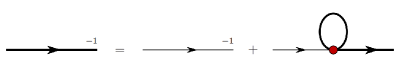
Figure 1: The NJL gap equation, formulated within the Hartree-Fock approximation, is depicted with a thin line representing the elementary quark propagator and a shaded circle denoting the $\bar{q}q$ interaction kernel. It is important to note that higher-order terms, such as those arising from meson loops, are not incorporated into the kernel of the gap equation.

II.2 The Off-shell Kaon GPDs

In the NJL model, the kaon off-shell GPDs are illustrated in Fig. 2. Here, $p$ represents the initial kaon momentum, while $p^{\prime}$ denotes the final kaon momentum. In the case of off-shell conditions where $p^{2}\neq p^{\prime 2}\neq m_{K}^{2}$, the kinematics and related quantities pertinent to this process are defined as follows:

$$t=q^{2}=(p^{\prime}-p)^{2}=-Q^{2},$$ (10)

$$P=\frac{p+p^{\prime}}{2},\quad\xi=\frac{p^{+}-p^{\prime+}}{p^{+}+p^{\prime+}},\quad n^{2}=0,$$ (11)

where $\xi$ represents the skewness parameter, and $n$ denotes the light-cone four-vector defined as $n=(1,0,0,-1)$ in the context of light-cone coordinates

$$v^{\pm} =(v^{0}\pm v^{3}),\quad\mathbf{v}=(v^{1},v^{2}),$$ (12)

for any four-vector $v^{+}$, it can be defined in light-cone coordinates as follows:

$$v^{+}=v\cdot n,$$ (13)

The vector and tensor quark GPDs of kaon are defined as

$$H^{q}(x,\xi,t,p^{2},p^{\prime 2}) =\frac{1}{2}\int\frac{dz^{-}}{2\pi}e^{\frac{i}{2}x(p^{+}+p^{\prime+})z^{-}}$$

$$\times\langle p^{\prime}|\bar{q}(-\frac{1}{2}z)\gamma^{+}q(\frac{1}{2}z)|p\rangle\mid_{z^{+}=0,\bm{z}=0},$$ (14)

$$\quad\frac{P^{+}q^{j}-P^{j}q^{+}}{P^{+}m_{K}}E^{q}(x,\xi,t,p^{2},p^{\prime 2})$$

$$=\frac{1}{2}\int\frac{dz^{-}}{2\pi}e^{\frac{i}{2}x(p^{+}+p^{\prime+})z^{-}}$$

$$\times\langle p^{\prime}|\bar{q}(-\frac{1}{2}z)i\sigma^{+j}q(\frac{1}{2}z)|p\rangle\mid_{z^{+}=0,\bm{z}=0},$$ (15)

where $x$ represents the longitudinal momentum fraction. The function $H^{q}(x,\xi,t,p^{2},p^{\prime 2})$ denotes the non-spin-flip or vector GPD, while $E^{q}(x,\xi,t,p^{2},p^{\prime 2})$ corresponds to the spin-flip or tensor GPD.

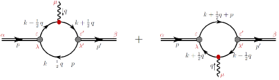
Figure 2: Diagrams of off-shell GPDs for kaons, where $p^{2}\neq p^{\prime 2}\neq m_{K}^{2}$.

The operators depicted in Fig. 2 for off-shell kaon GPDs are structured as follows:

$${\color[rgb]{1,0,0}\bullet}_{1} =\gamma^{+}\delta(x-\frac{k^{+}}{P^{+}})\,,$$ (16a)

$${\color[rgb]{1,0,0}\bullet}_{2} =i\sigma^{+j}\delta(x-\frac{k^{+}}{P^{+}}),$$ (16b)

where the first for vector GPD and the second for tensor GPD.

In the NJL model, the vector and tensor GPDs of the $u$ quark in the $K^{+}$ meson are defined as follows:

$$H^{u}\left(x,\xi,t,p^{2},p^{\prime 2}\right) =2iN_{c}Z_{K}\int\frac{d^{4}k}{(2\pi)^{4}}\delta_{n}^{x}(k)$$

$$\times\text{Tr}\left[\gamma_{5}S_{u}\left(k_{+}\right)\gamma^{+}S_{u}\left(k_{-}\right)\gamma_{5}S_{s}\left(k_{P}\right)\right],$$ (17)

$$\quad\frac{P^{+}q^{j}-P^{j}q^{+}}{P^{+}m_{K}}E^{u}\left(x,\xi,t,p^{2},p^{\prime 2}\right)$$

$$=2iN_{c}Z_{K}\int\frac{d^{4}k}{(2\pi)^{4}}\delta_{n}^{x}(k)$$

$$\times\text{Tr}\left[\gamma_{5}S_{u}\left(k_{+}\right)i\sigma^{+j}S_{u}\left(k_{-}\right)\gamma_{5}S_{s}\left(k_{P}\right)\right],$$ (18)

where $\delta_{n}^{x}(k)=\delta(xP^{+}-k^{+})$ $k_{+}=k+\frac{q}{2}$, $k_{-}=k-\frac{q}{2}$, $k_{P}=k-P$.

Here we use the notations

$$\mathcal{D}_{k_{+}}^{u} =\left(k+\frac{q}{2}\right)^{2}-M_{u}^{2}\,,$$ (19a)

$$\mathcal{D}_{k_{-}}^{u} =\left(k-\frac{q}{2}\right)^{2}-M_{u}^{2}\,,$$ (19b)

$$\mathcal{D}_{k_{P}}^{s} =\left(k-p-\frac{q}{2}\right)^{2}-M_{s}^{2},$$ (19c)

one can derive the following simplified formulas

$$p\cdot q =\frac{p^{\prime 2}-p^{2}-q^{2}}{2}\,,$$ (20a)

$$k\cdot q =\frac{1}{2}\left(\mathcal{D}_{k_{+}}^{u}-\mathcal{D}_{k_{-}}^{u}\right)\,,$$ (20b)

$$k\cdot p =-\frac{1}{2}\left(\mathcal{D}_{k_{P}}^{s}-\mathcal{D}_{k_{-}}^{u}-M_{u}^{2}+M_{s}^{2}-\frac{p^{\prime 2}+p^{2}-q^{2}}{2}\right)\,,$$ (20c)

$$k^{2} =\frac{1}{2}\left(\mathcal{D}_{k_{+}}^{u}+\mathcal{D}_{k_{-}}^{u}\right)+M_{u}^{2}-\frac{q^{2}}{4},$$ (20d)

after some calculation we arrive at

$$\quad H^{u}\left(x,\xi,t,p^{2},p^{\prime 2}\right)$$

$$=\frac{N_{c}Z_{K}}{8\pi^{2}}\left[\theta_{\bar{\xi}1}\bar{\mathcal{C}}_{1}(\sigma_{4})+\theta_{\xi 1}\bar{\mathcal{C}}_{1}(\sigma_{5})+\frac{\theta_{\bar{\xi}\xi}}{\xi}x\bar{\mathcal{C}}_{1}(\sigma_{6})\right]$$

$$+\frac{N_{c}Z_{K}}{8\pi^{2}}\int_{0}^{1}d\alpha\frac{\theta_{\alpha\xi}}{\xi}\frac{1}{\sigma_{7}}\bar{\mathcal{C}}_{2}(\sigma_{7})$$

$$\times((p^{\prime 2}-p^{2})\xi+(1-x)t+x(p^{2}+p^{\prime 2})-2x\left(M_{u}-M_{s}\right)^{2}),$$ (21)

$$E^{u}\left(x,\xi,t,p^{2},p^{\prime 2}\right)$$

$$= \frac{N_{c}Z_{K}}{4\pi^{2}}\int_{0}^{1}d\alpha\frac{\theta_{\alpha\xi}m_{K}}{\xi}((M_{s}-M_{u})\alpha+M_{u})\frac{\bar{\mathcal{C}}_{2}(\sigma_{7})}{\sigma_{7}},$$ (22)

and

$$\theta_{\bar{\xi}1} =x\in[-\xi,1]\,,$$ (23a)

$$\theta_{\xi 1} =x\in[\xi,1]\,,$$ (23b)

$$\theta_{\bar{\xi}\xi} =x\in[-\xi,\xi]\,,$$ (23c)

$$\theta_{\alpha\xi} =x\in[\alpha(\xi+1)-\xi,\alpha(1-\xi)+\xi]\cap x\in[-1,1].$$ (23d)

We denote the step function by $\theta$. It takes the value of $1$ in the corresponding region, and is otherwise equal to zero. These results pertain to the region where $\xi>0$. Under the transformation $\xi\rightarrow-\xi$, we observe that: $\theta_{\bar{\xi}1}\leftrightarrow\theta_{\xi 1}$; furthermore, both $\theta_{\bar{\xi}\xi}/\xi$ and $\theta_{\alpha\xi}/\xi$ remain invariant.

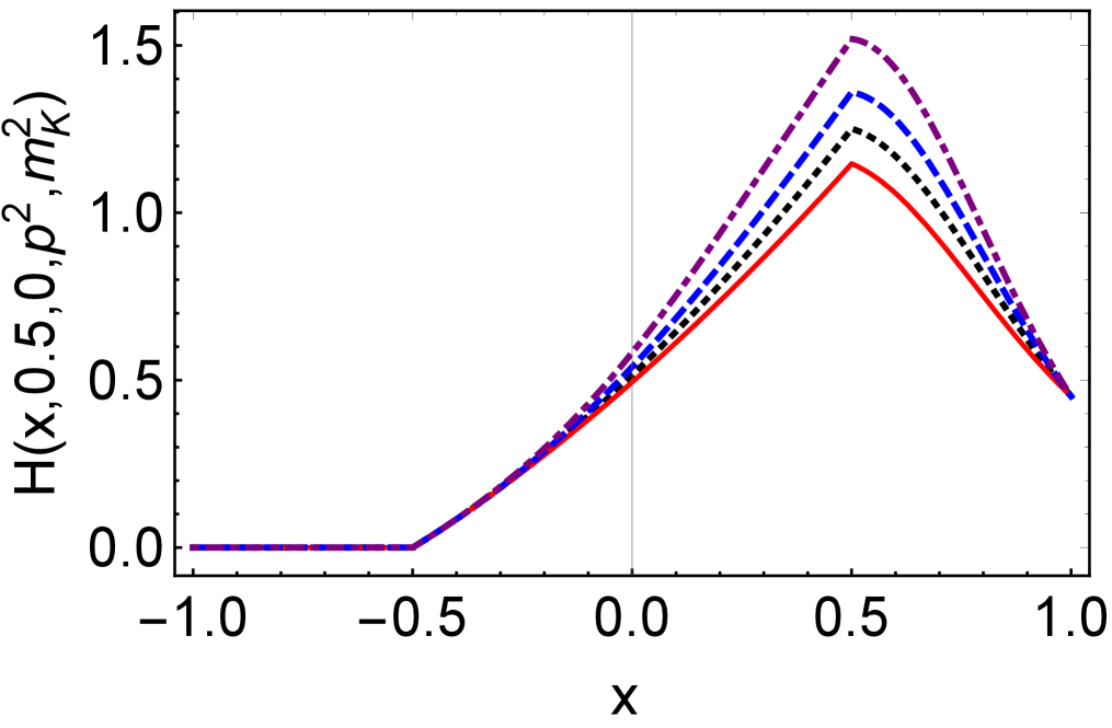
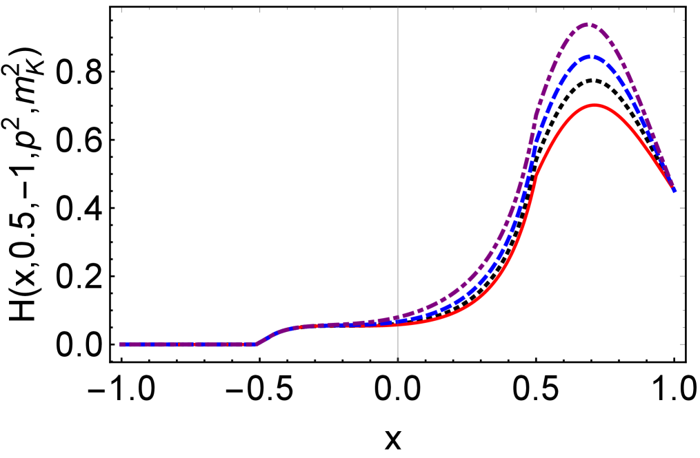
Figure 3: Kaon off-shell vector GPD: $H(x,\xi,t,p^{2},p^{\prime 2})$ in Eq. (II.2), we only plot $\xi>0$. upper panel – The off-shell GPDs $H(x,0.5,0,p^{2},m_{K}^{2})$. $H(x,0.5,0,m_{K}^{2},m_{K}^{2})$ – black dotted line; $H(x,0.5,0,0,m_{K}^{2})$ – red solid line; $H(x,0.5,0,0.4,m_{K}^{2})$ – blue dashed line; $H(x,0.5,0,0.6,m_{K}^{2})$ – purple dotdashed line. lower panel – The off-shell GPDs $H(x,0.5,-1,p^{2},m_{K}^{2})$. $H(x,0.5,-1,m_{K}^{2},m_{K}^{2})$ – black dotted line; $H(x,0.5,-1,0,m_{K}^{2})$ – red solid line; $H(x,0.5,0,-1,0.4,m_{K}^{2})$ – blue dashed line; $H(x,0.5,-1,0.6,m_{K}^{2})$ – purple dotdashed line.

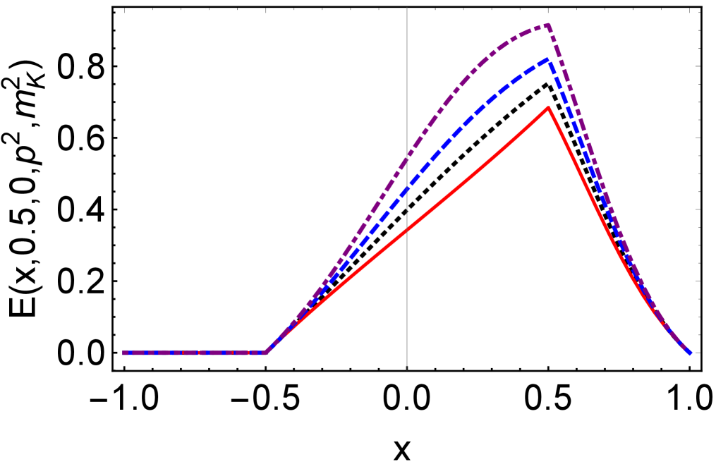
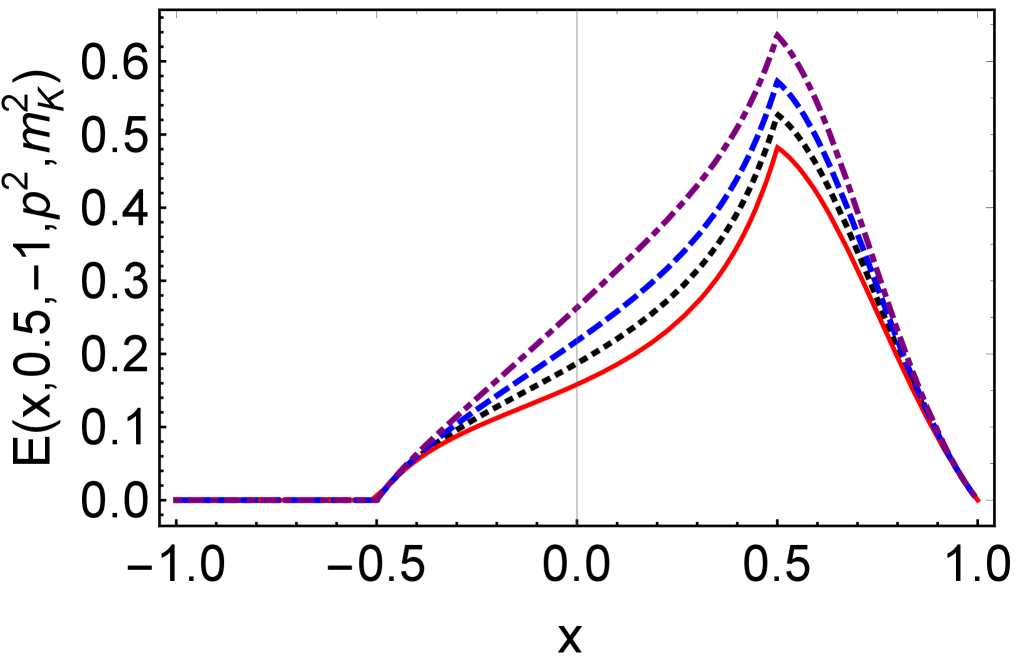
Figure 4: Pion off-shell tensor GPD: $E(x,\xi,t,p^{2},p^{\prime 2})$ in Eq. (II.2), we only plot $\xi>0$. upper panel – The off-shell GPDs $E(x,0.5,0,p^{2},m_{K}^{2})$. $H(x,0.5,0,m_{K}^{2},m_{K}^{2})$ – black dotted line; $E(x,0.5,0,0,m_{K}^{2})$ – red solid line; $E(x,0.5,0,0.4,m_{K}^{2})$ – blue dashed line; $E(x,0.5,0,0.6,m_{K}^{2})$ – purple dotdashed line. lower panel – The off-shell GPDs $E(x,0.5,0,p^{2},m_{K}^{2})$. $E(x,0.5,-1,m_{K}^{2},m_{K}^{2})$ – black dotted line; $E(x,0.5,-1,0,m_{K}^{2})$ – red solid line; $E(x,0.5,0,-1,0.4,m_{K}^{2})$ – blue dashed line; $E(x,0.5,-1,0.6,m_{K}^{2})$ – purple dotdashed line.

The diagrams of $H(x,\xi,t,p^{2},m_{\pi}^{2})$ and $E(x,\xi,t,p^{2},m_{\pi}^{2})$ are presented in Figs. 3 and 4. The off-shellness is influenced by $p^{2}$ at the condition where $p^{\prime 2}=m_{\pi}^{2}$. The diagrams illustrate that as $p^{2}$ increases, the off-shell effects of half-off-shell pion GPDs become increasingly pronounced. Specifically, at $p^{2}=0.4\text{GeV}^{2}$, this relative effect reaches approximately $10\%$, while at $p^{2}=0.6\text{GeV}^{2}$, it escalates to about $25\%$. These findings are consistent with those observed for off-shell pion GPDs.

II.3 The Properties of Kaon off-shell GPDs

II.3.1 Forward Limit

In the case the initial and final kaon have the same momentum $p=p^{\prime}$, which means $\xi=0$, $t=0$, vector GPD reduces to kaon PDF,

$$\quad u_{K}(x,p^{2})$$

$$=\frac{3Z_{K}}{4\pi^{2}}\bar{\mathcal{C}}_{1}(\sigma_{1})$$

$$+\frac{3Z_{K}}{2\pi^{2}}x(1-x)(p^{2}-\left(M_{u}-M_{s}\right)^{2})\frac{\bar{\mathcal{C}}_{2}(\sigma_{1})}{\sigma_{1}},$$ (24)

when the skewness parameter $\xi=0$, the function $H^{u}(x,0,0,p^{2},p^{2})$ vanishes in the region where $x\in[-1,0]$. In contrast, for the region where $x\in[0,1]$, this off-shell PDF of the $u$ quark in kaons differs from that of pions as described in the NJL model Zhang et al. (2021c); Zhang (2025b).

In Fig. 5, we present the diagram of the off-shell $u$ quark PDF. It is evident that when $p^{2}=0$ and $p^{2}=m_{K}^{2}$, the lines are nearly straight. As $p^{2}$ increases, particularly in the context of an off-shell kaon, a more pronounced dependence on $x$ emerges. The NJL model effectively describes low-energy properties within QCD. At high values of $Q^{2}$, however, evolution becomes necessary; consequently, the dependence on $x$ will vary as a result of this evolution. Different from the pion PDF, the position of $x$ corresponding to the maximum value of the function has shifted to a region where $x$ is less than $0.5$.

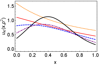
Figure 5: The off-shell $u$ quark PDFs of kaon: $u\left(x,p^{2}\right)$ with $p^{2}=0$ GeV² — orange dotted curve, $p^{2}=m_{K}^{2}=0.47^{2}$ GeV² — red solid curve, $p^{2}=0.4$ GeV^-2 — blue dashed curve, $p^{2}=0.6$ GeV² — purple dot-dashed curve, $p^{2}=0.8$ GeV² — black solid thick curve.

II.3.2 Polynomiality Condition

The $x$-moments of the off-shell GPDs also include odd powers of the skewness parameter $\xi$.

$$\int_{-1}^{1}x^{n}H^{q}(x,\xi,t,p^{2},p^{\prime 2})dx =\sum_{i=0}^{(n+1)}A_{n,i}(t,p,p^{\prime})\xi^{i}\,,$$ (25a)

$$\int_{-1}^{1}x^{n}dxE^{q}(x,\xi,t,p^{2},p^{\prime 2})dx =\sum_{i=0}^{(n+1)}B_{n,i}^{q}(t,p^{2},p^{\prime 2})\xi^{i}.$$ (25b)

When $n=0$, we obtain FFs

$$\int_{-1}^{1}x^{0}H^{u}dx =A_{1,0}^{u}+\xi A_{1,1}^{u}=F^{u}-G^{u}\xi\,,$$ (26a)

$$\int_{-1}^{1}x^{0}E^{u}dx =B_{1,0}^{u}+\xi B_{1,1}^{u},$$ (26b)

where $A_{1,0}^{u}$ and $B_{1,0}^{u}$ are the $u$ quark vector and tensor FFs. $A_{1,1}^{u}$ and $B_{1,1}^{u}$ are FFs due to the off-shellness. $A_{1,0}^{u}$ and $B_{1,0}^{u}$ are symmetry about the $p$ and $p^{\prime}$, but $A_{1,1}^{u}$ and $B_{1,1}^{u}$ are antisymmetry about $p$ and $p^{\prime}$.

The functions $F(t,p^{2},p^{\prime 2})$ and $G(t,p^{2},p^{\prime 2})$ are defined in the general covariant structure of the kaon-photon vertex:

$$\Gamma^{\mu}(p,p^{\prime})=2P^{\mu}F(t,p^{2},p^{\prime 2})+q^{\mu}G(t,p^{2},p^{\prime 2}),$$ (27)

at $t=0$, the relationship Broniowski et al. (2023b)

$$G(t,p^{2},p^{\prime 2})=\frac{(p^{\prime 2}-p^{2})}{t}\left[F(0,p^{2},p^{\prime 2})-F(t,p^{2},p^{\prime 2})\right],$$ (28)

where $G(0,p^{2},p^{\prime 2})=(p^{\prime 2}-p^{2})dF(t,p^{2},p^{\prime 2})/dt|_{t=0}$ indicates that, due to crossing symmetry, one can conclude that $G(t,p^{2},p^{2})=0$. Here, $F(t,p^{2},p^{\prime 2})$ represents the electromagnetic FFs, and it is noted that $F(0,m_{K}^{2},m_{K}^{2})=1$. From the off-shell kaon GPDs, one can derive

$$\quad A_{1,0}^{u}(Q^{2},p^{2},p^{\prime 2})$$

$$=\frac{N_{c}Z_{K}}{8\pi^{2}}\int_{0}^{1}dx\,\bar{\mathcal{C}}_{1}(\sigma_{1})+\frac{N_{c}Z_{K}}{8\pi^{2}}\int_{0}^{1}dx\,\bar{\mathcal{C}}_{1}(\sigma_{2})$$

$$+\frac{N_{c}Z_{K}}{4\pi^{2}}\int_{0}^{1}dx\int_{0}^{1-x}dy\frac{1}{\sigma_{8}}\bar{\mathcal{C}}_{2}(\sigma_{8})$$

$$\times((1-x-y)((p^{2}+p^{\prime 2})-2(M_{u}^{2}-M_{s})^{2})-(x+y)Q^{2}),$$ (29)

$$\quad A_{1,1}^{u}(Q^{2},p^{2},p^{\prime 2})$$

$$=\frac{N_{c}Z_{K}}{8\pi^{2}}\int_{0}^{1}dx\,\bar{\mathcal{C}}_{1}(\sigma_{1})-\frac{N_{c}Z_{K}}{8\pi^{2}}\int_{0}^{1}dx\,\bar{\mathcal{C}}_{1}(\sigma_{2})$$

$$-\frac{N_{c}Z_{K}}{4\pi^{2}}\int_{0}^{1}dx\int_{0}^{1-x}dy(p^{2}-p^{\prime 2})\frac{\bar{\mathcal{C}}_{2}(\sigma_{8})}{\sigma_{8}}$$

$$-\frac{N_{c}Z_{K}}{4\pi^{2}}\int_{0}^{1}dx\int_{0}^{1-x}dy\frac{\bar{\mathcal{C}}_{2}(\sigma_{8})}{\sigma_{8}}$$

$$\times((p^{2}-p^{\prime 2})+(y-x)(p^{2}+p^{\prime 2}+Q-2(M_{u}-M_{s})^{2})),$$ (30)

$$\quad B_{1,0}^{u}(Q^{2},p^{2},p^{\prime 2})$$

$$=\frac{N_{c}Z_{K}}{2\pi^{2}}\int_{0}^{1}dx\int_{0}^{1-x}dy$$

$$\times m_{K}\left((M_{s}-M_{u})(1-x-y)+M_{u}\right)\frac{\bar{\mathcal{C}}_{2}(\sigma_{8})}{\sigma_{8}},$$ (31)

where $B_{1,1}^{u}(Q^{2},p^{2},p^{\prime 2})=0$.

We demonstrate that our $A_{1,1}^{u}(Q^{2},p^{2},p^{\prime 2})$ is equivalent to $-G^{u}(Q^{2},p^{2},p^{\prime 2})$ as presented in Eq. (28), consistent with the findings of Ref. Broniowski et al. (2023b).

For $n=1$, GPDs should follow the sum rule:

$$\quad\int_{-1}^{1}x\,dxH^{u}(x,\xi,t,p^{2},p^{\prime 2})$$

$$=A_{2,0}^{u}(t,p^{2},p^{\prime 2})+\xi A_{2,1}^{u}(t,p^{2},p^{\prime 2})+\xi^{2}A_{2,2}^{u}(t,p^{2},p^{\prime 2})$$

$$=\theta_{2}^{u}(t,p^{2},p^{\prime 2})-\xi\theta_{3}^{u}(t,p^{2},p^{\prime 2})-\xi^{2}\theta_{1}^{u}(t,p^{2},p^{\prime 2})\,,$$ (32a)

$$\quad\int_{-1}^{1}x\,dxE^{u}(x,\xi,t,p^{2},p^{\prime 2})$$

$$=B_{2,0}^{u}(t,p^{2},p^{\prime 2})+\xi B_{2,1}^{u}(t,p^{2},p^{\prime 2})+\xi^{2}B_{2,2}^{u}(t,p^{2},p^{\prime 2}),$$ (32b)

where $\theta_{2}^{u}$ pertains to the mass distribution of the $u$ quark within the kaon, while $\theta_{1}^{u}$ is associated with the pressure distribution of the $u$ quark. The polynomial contains only the terms $\xi^{0}$ and $\xi^{2}$, thereby satisfying Eqs. (25). The generalized FFs for $n=1$ are as follows:

$$A_{2,0}^{u}(Q^{2},p^{2},p^{\prime 2})$$

$$= \frac{N_{c}Z_{K}}{8\pi^{2}}\int_{0}^{1}dxx\bar{\mathcal{C}}_{1}(\sigma_{1})+\frac{N_{c}Z_{K}}{8\pi^{2}}\int_{0}^{1}dxx\bar{\mathcal{C}}_{1}(\sigma_{2})$$

$$+ \frac{N_{c}Z_{K}}{4\pi^{2}}\int_{0}^{1}dx\int_{0}^{1-x}dy(1-x-y)\frac{1}{\sigma_{8}}\bar{\mathcal{C}}_{2}(\sigma_{8})$$

$$\times (((p^{2}+p^{\prime 2})-2(M_{s}-M_{u})^{2})(1-x-y)-Q^{2}(x+y)),$$ (33)

$$A_{2,1}=\frac{N_{c}Z_{K}}{8\pi^{2}}\left(\frac{1}{p^{2}}-\frac{1}{p^{\prime 2}}\right)(\mathcal{C}_{0}(M_{u}^{2})-\mathcal{C}_{0}(M_{s}^{2}))$$

$$+\frac{N_{c}Z_{K}}{8\pi^{2}}\int_{0}^{1}dx\bar{\mathcal{C}}_{1}(\sigma_{1})$$

$$\times\left(2x-1+\frac{2x(p^{2}+p^{\prime 2}-2(M_{u}-M_{s})^{2})}{Q^{2}}-\frac{M_{s}^{2}-M_{u}^{2}}{p^{2}}\right)$$

$$-\frac{N_{c}Z_{K}}{8\pi^{2}}\int_{0}^{1}dx\bar{\mathcal{C}}_{1}(\sigma_{2})$$

$$\times\left(2x-1+\frac{2x(p^{2}+p^{\prime 2}-2(M_{u}-M_{s})^{2})}{Q^{2}}-\frac{M_{s}^{2}-M_{u}^{2}}{p^{\prime 2}}\right)$$

$$+\frac{N_{c}Z_{K}}{2\pi^{2}}\int_{0}^{1}dx\int_{0}^{1-x}dy(1-x-y)(p^{\prime 2}-p^{2})\frac{\bar{\mathcal{C}}_{2}(\sigma_{8})}{\sigma_{8}}$$

$$\times\left((x+y)-\frac{(p^{\prime 2}+p^{2}-2(M_{u}-M_{s})^{2})(1-x-y)}{Q^{2}}\right),$$ (34)

$$A_{2,2}=-\frac{N_{c}Z_{K}}{2\pi^{2}}\int_{0}^{1}dxx(1-2x)\bar{\mathcal{C}}_{1}(\sigma_{3})$$

$$+\frac{N_{c}Z_{K}}{8\pi^{2}}\int_{0}^{1}dx(\bar{\mathcal{C}}_{1}(\sigma_{2})-\bar{\mathcal{C}}_{1}(\sigma_{1}))(p^{2}-p^{\prime 2})$$

$$\times\left(\frac{x-1}{Q^{2}}+\frac{x(p^{\prime 2}+p^{2}-2(M_{u}-M_{s})^{2})}{Q^{4}}\right)$$

$$+\frac{N_{c}Z_{\pi}}{8\pi^{2}}\int_{0}^{1}dx(\bar{\mathcal{C}}_{1}(\sigma_{2})+\bar{\mathcal{C}}_{1}(\sigma_{1}))$$

$$\times(1-x)\frac{(p^{\prime 2}+p^{2}-2(M_{u}-M_{s})^{2})}{Q^{2}}$$

$$-\frac{N_{c}Z_{K}}{4\pi^{2}}\int_{0}^{1}dx\int_{0}^{1-x}dy\bar{\mathcal{C}}_{1}(\sigma_{8})$$

$$\times\left(\frac{(p^{\prime 2}+p^{2}-2(M_{u}-M_{s})^{2})}{Q^{2}}+1\right)$$

$$+\frac{N_{c}Z_{K}}{4\pi^{2}}\int_{0}^{1}dx\int_{0}^{1-x}dy(1-x-y)(p^{\prime 2}-p^{2})^{2}\frac{\bar{\mathcal{C}}_{2}(\sigma_{8})}{\sigma_{8}}$$

$$\times\left(\frac{(p^{\prime 2}+p^{2}-2(M_{u}-M_{s})^{2})(1-x-y)}{Q^{4}}-\frac{(x+y)}{Q^{2}}\right),$$ (35)

$$B_{2,0}^{u}(Q^{2},p^{2},p^{\prime 2})$$

$$= \frac{N_{c}Z_{K}}{2\pi^{2}}\int_{0}^{1}dx\int_{0}^{1-x}dy\frac{1}{\sigma_{8}}\bar{\mathcal{C}}_{2}(\sigma_{8})$$

$$\times m_{K}((1-x-y)^{2}(M_{s}-M_{u})+(1-x-y)M_{u}),$$ (36)

$$\quad B_{2,1}^{u}(Q^{2},p^{2},p^{\prime 2})$$

$$=-\frac{N_{c}Z_{K}}{4\pi^{2}}\int_{0}^{1}dx\frac{m_{K}(x(M_{s}-M_{u})+M_{u})}{Q^{2}}\bar{\mathcal{C}}_{1}(\sigma_{1})$$

$$+\frac{N_{c}Z_{K}}{4\pi^{2}}\int_{0}^{1}dx\frac{m_{K}(x(M_{s}-M_{u})+M_{u})}{Q^{2}}\bar{\mathcal{C}}_{1}(\sigma_{2})$$

$$-\frac{N_{c}Z_{K}}{2\pi^{2}}\int_{0}^{1}dx\int_{0}^{1-x}dy(1-x-y)\frac{\bar{\mathcal{C}}_{2}(\sigma_{8})}{\sigma_{8}}$$

$$\times m_{K}((1-x-y)(M_{s}-M_{u})+M_{u})\frac{(p^{\prime 2}-p^{2})}{Q^{2}}.$$ (37)

For the $u$ quark tensor GPD $E^{u}(x,\xi,t,p^{2},p^{\prime 2})$ of the kaon within the NJL model, it is noted that $B_{2,2}^{u}(Q^{2},p^{2},p^{\prime 2})=0$.

II.3.3 Impact Parameter Denpendent PDFs

The impact parameter dependent PDFs are given by,

$$\quad q\left(x,\bm{b}_{\perp}^{2},p^{2},p^{\prime 2}\right)$$

$$=\int\frac{d^{2}\bm{q}_{\perp}}{(2\pi)^{2}}e^{-i\bm{b}_{\perp}\cdot\bm{q}_{\perp}}H^{q}\left(x,0,-\bm{q}_{\perp}^{2},p^{2},p^{\prime 2}\right).$$ (38)

This means that the impact parameter dependent PDFs defined above are the Fourier transform of $H^{u}\left(x,0,-\bm{q}_{\perp}^{2}\right)$, therefore, when we obtain $H^{u}\left(x,0,-\bm{q}_{\perp}^{2}\right)$, parton distribution as a function of the distance $\bm{b}_{\perp}$ and the light-cone momentum fraction $x$ can be determined.

When $\xi\rightarrow 0$ and $t\neq 0$, GPDs become

$$\quad H^{u}\left(x,0,-\bm{q}_{\perp}^{2},p^{2},p^{\prime 2}\right)$$

$$=\frac{3Z_{K}}{8\pi^{2}}(\bar{\mathcal{C}}_{1}(\sigma_{1})+\bar{\mathcal{C}}_{1}(\sigma_{2}))$$

$$+\frac{3Z_{K}}{4\pi^{2}}\int_{0}^{1-x}d\alpha\frac{1}{\sigma_{9}}\bar{\mathcal{C}}_{2}(\sigma_{9})$$

$$\times((x-1)\bm{q}_{\perp}^{2}+x((p^{\prime 2}+p^{2})-2(M_{u}-M_{s})^{2})),$$ (39)

$$\quad E^{u}\left(x,0,-\bm{q}_{\perp}^{2},p^{2},p^{\prime 2}\right)$$

$$=\frac{N_{c}Z_{K}}{2\pi^{2}}\int_{0}^{1-x}d\alpha\,m_{K}((M_{s}-M_{u})\alpha+M_{u})\frac{\bar{\mathcal{C}}_{2}(\sigma_{9})}{\sigma_{9}},$$ (40)

where $x$ is defined within the interval $x\in[0,1]$, we can derive the following:

$$u_{K}\left(x,\bm{b}_{\perp}^{2},p^{2},p^{\prime 2}\right) =\frac{N_{c}Z_{K}}{8\pi^{2}}\int\frac{d^{2}\bm{q}_{\perp}}{(2\pi)^{2}}e^{-i\bm{b}_{\perp}\cdot\bm{q}_{\perp}}(\bar{\mathcal{C}}_{1}(\sigma_{1})+\bar{\mathcal{C}}_{1}(\sigma_{2}))$$

$$+\frac{N_{c}Z_{K}}{32\pi^{3}}\int_{0}^{1-x}d\alpha\int d\tau\left(\frac{(x-1)+\alpha\tau x(1-\alpha-x)((p^{\prime 2}+p^{2})-2(M_{u}-M_{s})^{2})}{\alpha^{2}\tau^{2}(1-\alpha-x)^{2}}+\frac{(x-1)\bm{b}_{\perp}^{2}}{4\alpha^{3}\tau^{3}(1-\alpha-x)^{3}}\right)$$

$$\times e^{-\tau\left((1-x)M_{u}^{2}+xM_{s}^{2}-(x\alpha p^{2}+x(1-\alpha-x)p^{\prime 2})\right)}e^{-\frac{\bm{b}_{\perp}^{2}}{4\tau\alpha(1-\alpha-x)}},$$ (41)

$$u_{K}^{T}\left(x,\bm{b}_{\perp}^{2},p^{2},p^{\prime 2}\right) =\frac{N_{c}Z_{K}}{16\pi^{3}}\int_{0}^{1-x}d\alpha\int d\tau\frac{m_{K}((M_{s}-M_{u})\alpha+M_{u})}{\alpha\left(1-\alpha-x\right)\tau}e^{-\frac{1}{4\tau(1-\alpha-x)\alpha}\bm{b}_{\perp}^{2}}e^{-\tau\left((1-x)M_{u}^{2}+xM_{s}^{2}-(x\alpha p^{2}+x(1-\alpha-x)p^{\prime 2})\right)},$$ (42)

when integrating $\bm{b}_{\perp}$, we can obtain the $u$ quark PDF as presented in Eq. (II.3.1).

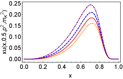
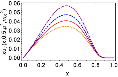
Figure 6: Impact parameter space PDFs : upper panel – $xu\left(x,0.5,p^{2},m_{\pi}^{2}\right)$, the $\delta^{2}(\bm{b}_{\perp})$ component first line of Eq. (II.3.3) – is suppressed in the image, and lower panel – $xu_{T}\left(x,0.5,p^{2},m_{\pi}^{2}\right)$ both panels with $p^{2}=0$ GeV² — orange dotted curve, $p^{2}=0.14^{2}$ GeV² — red solid curve, $p^{2}=0.2$ GeV^-2 — blue dashed curve, $p^{2}=0.4$ GeV² — purple dot-dashed curve.

Fig. 6 illustrates the off-shell impact parameter space PDFs multiplied by $x$ at $\bm{b}_{\perp}^{2}=0.5$ GeV^-2 for various values of $p^{2}$. From the diagram, it is evident that the maximum value of $xu\left(x,0.5,p^{2},m_{\pi}^{2}\right)$ corresponds to a larger value of $x$ compared to that associated with the maximum value of $xu_{T}\left(x,0.5,p^{2},m_{\pi}^{2}\right)$. As the value of $p^{2}$ increases, the maximum values of $xu\left(x,0.5,p^{2},m_{\pi}^{2}\right)$ and $xu_{T}\left(x,0.5,p^{2},m_{\pi}^{2}\right)$ also rise. Concurrently, with the increase in $p^{2}$, the position $x$ that corresponds to the maximum value of $xu\left(x,0.5,p^{2},m_{\pi}^{2}\right)$ decreases, while maintaining a coordinate where $x>0.5$. In contrast, for $xu_{T}\left(x,0.5,p^{2},m_{\pi}^{2}\right)$, as $p^{2}$ increases, the position of $x$ corresponding to its maximum values remains relatively unchanged, hovering around approximately $x=0.5$.

III The kaon off-shell TMDs

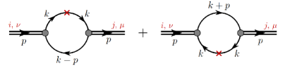
Figure 7: Feynman diagrams illustrating the kaon TMDs within the NJL model are presented. The shaded circles denote the kaon Bethe-Salpeter vertex functions, while the solid lines represent the dressed quark propagator. The operator insertion takes the form $\gamma^{+}\delta(x-\frac{k^{+}}{p^{+}})$. The left diagram corresponds to the TMDs of the up $u$ quark, whereas the right diagram pertains to those of the strange $s$ quark in relation to the kaon.

The kaon TMD is depicted in Fig. 7. Within the context of the Nambu-Jona-Lasinio (NJL) model, it is defined as follows:

$$\langle\Gamma\rangle(x,\bm{k}_{\perp}^{2})=-\frac{iN_{c}Z_{K}}{p^{+}}\int\frac{\mathrm{d}k^{+}\mathrm{d}k^{-}}{(2\pi)^{4}}\delta(x-\frac{k^{+}}{p^{+}})$$

$$\times\text{tr}_{\text{D}}\left[\gamma^{5}S_{u}\left(k\right)\gamma^{+}S_{u}\left(k\right)\gamma^{5}S_{s}\left(k-p\right)\right],$$ (43)

where $\text{tr}_{\text{D}}$ represents a trace over spinor indices. As a result, we have successfully derived the final expression for the off-shell kaon TMD.

$$\quad f(x,\bm{k}_{\perp}^{2},p^{2})$$

$$=\frac{N_{c}Z_{K}}{2\pi^{3}}\frac{\bar{\mathcal{C}}_{2}(\sigma_{10})}{\sigma_{10}}$$

$$+\frac{N_{c}Z_{K}}{4\pi^{3}}x(1-x)(p^{2}-(M_{u}-M_{s})^{2})\frac{6\bar{\mathcal{C}}_{3}(\sigma_{10})}{\sigma_{10}^{2}},$$ (44)

in Fig. 8, we plot a three-dimensional diagram of the on-shell and off-shell kaon TMD at $p^{2}=0.6$ GeV². For the on-shell case, it is evident that as $x\rightarrow 0$, the function $f(x,\bm{k}_{\perp}^{2})$ reaches its maximum value. This behavior contrasts with that of the pion on-shell TMD. The off-shell TMD exhibits a more pronounced dependence on $x$, resembling the characteristics of the pion off-shell TMD. However, it is noteworthy that the value of $x$ corresponding to the maximum has shifted to a position less than $0.5$, which distinguishes it from both the pion on-shell and off-shell TMDs, as those are symmetric about $x=0.5$. The off-shell kaon PDF as articulated in Eq. (II.3.1) can be derived through the integration over $\bm{k}_{\perp}$.

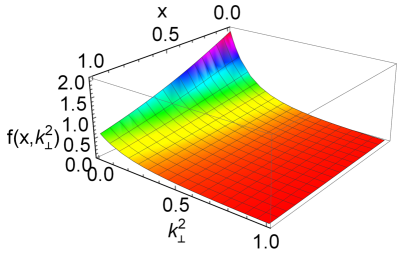
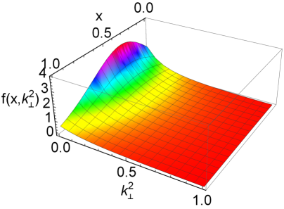
Figure 8: Kaon TMDs: Upper Panel – The on-shell kaon TMDs represented as $f(x,\bm{k}_{\perp}^{2},m_{K}^{2})$; Lower Panel – The off-shell kaon TMDs denoted by $f(x,\bm{k}_{\perp}^{2},0.6)$

IV Summary and Outlook

In this paper, we investigate the off-shell generalized parton distributions (GPDs) and transverse momentum dependent parton distributions (TMDs) of kaons within the framework of the Nambu–Jona-Lasinio (NJL) model, employing proper time regularization. We derive off-shell form factors (FFs), off-shell parton distribution functions (PDFs), and impact parameter-dependent PDFs. Subsequently, we compare these distributions with their on-shell counterparts and examine their properties.

Unlike on-shell GPDs, the lack of crossing symmetry in off-shell GPDs results in their Mellin moments exhibiting not only even powers of the skewness parameter but also odd powers. This indicates the emergence of new off-shell FFs. Our findings indicate the modifications in kaon GPDs resulting from off-shell effects. Unlike their on-shell counterparts, certain properties may not hold in the off-shell scenario; for instance, symmetry properties and polynomiality conditions may no longer be applicable.

For the off-shell kaon GPDs, the relative off-shell effect ranges from approximately $15\%$ to $25\%$. We have also conducted a comparison between the off-shell kaon GPDs and those of pions. By analyzing the Mellin moments of kaon GPDs, we derive both the off-shell FFs and gravitational FFs. Furthermore, we compare the off-shell FFs of kaons with those of pions.

In summary, the NJL model has been demonstrated to effectively describe the off-shell characteristics of pion and kaon structures. In future work, we can extend these calculations to encompass the off-shell GPDs and FFs of vector mesons such as $\rho$ and $K^{*}$, as well as protons and neutrons. Furthermore, we can replicate the results for off-shell GPDs obtained in this study using models that incorporate more realistic interactions; this may provide additional insights into the underlying physics.

Appendix A APPENDIX 1: USEFUL FORMULAE

Here we use the gamma-functions ($n\in\mathbb{Z}$, $n\geq 0$)

$$\mathcal{C}_{0}(z) =\int_{0}^{\infty}ds\,s\int_{\tau_{uv}^{2}}^{\tau_{ir}^{2}}d\tau e^{-\tau(s+z)}$$

$$=z[\Gamma(-1,z\tau_{uv}^{2})-\Gamma(-1,z\tau_{ir}^{2})]\,,$$ (45a)

$$\mathcal{C}_{n}(z) =(-)^{n}\frac{\sigma^{n}}{n!}\frac{d^{n}}{d\sigma^{n}}\mathcal{C}_{0}(\sigma)\,,$$ (45b)

$$\bar{\mathcal{C}}_{i}(z) =\frac{1}{z}\mathcal{C}_{i}(z).$$ (45c)

where $\tau_{uv,ir}=1/\Lambda_{\text{UV},\text{IR}}$ are, respectively, the infrared and ultraviolet regulators described above.

The functions denoted by $\sigma$ are defined as follows:

$$\sigma_{1} =(1-x)M_{u}^{2}+xM_{s}^{2}-x(1-x)p^{2}\,,$$ (46a)

$$\sigma_{2} =(1-x)M_{u}^{2}+xM_{s}^{2}-x(1-x)p^{\prime 2}\,,$$ (46b)

$$\sigma_{3} =M_{u}^{2}-x(1-x)t\,,$$ (46c)

$$\sigma_{4} =\frac{1-x}{1+\xi}M_{u}^{2}+\frac{x+\xi}{1+\xi}M_{s}^{2}-\frac{x+\xi}{1+\xi}\frac{1-x}{1+\xi}p^{2}\,,$$ (46d)

$$\sigma_{5} =\frac{1-x}{1-\xi}M_{u}^{2}+\frac{x-\xi}{1-\xi}M_{s}^{2}-\frac{x-\xi}{1-\xi}\frac{1-x}{1-\xi}p^{\prime 2}\,,$$ (46e)

$$\sigma_{6} =M_{u}^{2}-\frac{1}{4}(1+\frac{x}{\xi})(1-\frac{x}{\xi})t\,,$$ (46f)

$$\sigma_{7} =(1-\alpha)M_{u}^{2}+\alpha M_{s}^{2}$$

$$-\alpha\left(\left(\frac{\xi-x}{2\xi}+\alpha\frac{1-\xi}{2\xi}\right)p^{2}+\left(\frac{\xi+x}{2\xi}-\alpha\frac{1+\xi}{2\xi}\right)p^{\prime 2}\right)$$

$$-\left(\frac{\xi+x}{2\xi}-\alpha\frac{1+\xi}{2\xi}\right)\left(\frac{\xi-x}{2\xi}+\alpha\frac{1-\xi}{2\xi}\right)t\,,$$ (46g)

$$\sigma_{8} =x(x-1)p^{\prime 2}+y(y-1)p^{2}+xy(p^{2}+p^{\prime 2})$$

$$+(x+y)M_{u}^{2}+(1-x-y)M_{s}^{2}\,,$$ (46h)

$$\sigma_{9} =(1-x)M_{u}^{2}+xM_{s}^{2}+(1-\alpha-x)\alpha\bm{q}_{\perp}^{2}$$

$$-(x\alpha p^{2}+x(1-\alpha-x)p^{\prime 2})\,,$$ (46i)

$$\sigma_{10} =\bm{k}_{\bot}^{2}+(1-x)M_{u}^{2}+xM_{s}^{2}-x(1-x)p^{2},$$ (46j)

References

- Xu et al. (2025) Z.-N. Xu, D. Binosi, C. Chen, K. Raya, C. D. Roberts, and J. Rodríguez-Quintero, Phys. Lett. B 865, 139451 (2025), arXiv:2411.15376 [hep-ph] .
- Wu et al. (2025) Q. Wu, Z.-F. Cui, and J. Segovia, Phys. Rev. D 111, 116023 (2025), arXiv:2503.07055 [hep-ph] .
- Tanisha et al. (2025) Tanisha, S. Puhan, A. Yadav, and H. Dahiya, (2025), arXiv:2505.09213 [hep-ph] .
- Muller et al. (1994) D. Muller, D. Robaschik, B. Geyer, F. M. Dittes, and J. Horejsi, Fortsch. Phys. 42, 101 (1994), arXiv:hep-ph/9812448 [hep-ph] .
- Ji (1997) X.-D. Ji, Phys. Rev. D 55, 7114 (1997), arXiv:hep-ph/9609381 .
- Radyushkin (1997) A. V. Radyushkin, Phys. Rev. D 56, 5524 (1997), arXiv:hep-ph/9704207 .
- Ji (1998) X.-D. Ji, J. Phys. G 24, 1181 (1998), arXiv:hep-ph/9807358 .
- Theussl et al. (2004) L. Theussl, S. Noguera, and V. Vento, Eur. Phys. J. A 20, 483 (2004), arXiv:nucl-th/0211036 .
- Diehl (2003) M. Diehl, Phys. Rept. 388, 41 (2003), arXiv:hep-ph/0307382 .
- Zhang et al. (2021a) J.-L. Zhang, Z.-F. Cui, J. Ping, and C. D. Roberts, Eur. Phys. J. C 81, 6 (2021a), arXiv:2009.11384 [hep-ph] .
- Zhang et al. (2021b) J.-L. Zhang, K. Raya, L. Chang, Z.-F. Cui, J. M. Morgado, C. D. Roberts, and J. Rodríguez-Quintero, Phys. Lett. B 815, 136158 (2021b), arXiv:2101.12286 [hep-ph] .
- Zhang et al. (2021c) J.-L. Zhang, M.-Y. Lai, H.-S. Zong, and J.-L. Ping, Nucl. Phys. B 966, 115387 (2021c).
- Zhang and Ping (2021) J.-L. Zhang and J.-L. Ping, Eur. Phys. J. C 81, 814 (2021).
- Zhang et al. (2022a) J.-L. Zhang, G.-Z. Kang, and J.-L. Ping, Chin. Phys. C 46, 063105 (2022a), arXiv:2110.06463 [hep-ph] .
- Zhang et al. (2022b) J.-L. Zhang, G.-Z. Kang, and J.-L. Ping, Phys. Rev. D 105, 094015 (2022b), arXiv:2204.14032 [hep-ph] .
- Mezrag (2022) C. Mezrag, Few Body Syst. 63, 62 (2022), arXiv:2207.13584 [hep-ph] .
- Qiu and Yu (2022) J.-W. Qiu and Z. Yu, JHEP 08, 103 (2022), arXiv:2205.07846 [hep-ph] .
- Zhang (2024) J.-L. Zhang, (2024), arXiv:2409.04105 [hep-ph] .
- Goharipour et al. (2025) M. Goharipour, M. H. Amiri, F. Irani, H. Hashamipour, and K. Azizi (MMGPDs), (2025), arXiv:2508.15073 [hep-ph] .
- Zhang (2025a) J.-L. Zhang, Chin. Phys. C 49, 043104 (2025a), arXiv:2409.19525 [hep-ph] .
- Bondarenko and Slautin (2025) S. Bondarenko and M. Slautin, (2025), arXiv:2506.22153 [hep-ph] .
- Hernández-Pinto et al. (2024) R. J. Hernández-Pinto, L. X. Gutiérrez-Guerrero, M. A. Bedolla, and A. Bashir, Phys. Rev. D 110, 114015 (2024), arXiv:2410.23813 [hep-ph] .
- Puhan and Dahiya (2025) S. Puhan and H. Dahiya, Phys. Rev. D 111, 114039 (2025), arXiv:2505.02507 [hep-ph] .
- Cheng et al. (2025) P. Cheng, Z.-Q. Yao, D. Binosi, and C. D. Roberts, Phys. Lett. B 862, 139323 (2025), arXiv:2412.10598 [hep-ph] .
- Zhang and Wu (2024) J.-L. Zhang and J. Wu, Chin. Phys. C 48, 083106 (2024), arXiv:2402.12757 [hep-ph] .
- Ji and Yang (2025) X. Ji and C. Yang, (2025), arXiv:2508.16727 [hep-ph] .
- Goeke et al. (2001) K. Goeke, M. V. Polyakov, and M. Vanderhaeghen, Prog. Part. Nucl. Phys. 47, 401 (2001), arXiv:hep-ph/0106012 .
- Radyushkin (1996) A. V. Radyushkin, Phys. Lett. B 380, 417 (1996), arXiv:hep-ph/9604317 .
- Hobart (2023) A. Hobart (CLAS), EPJ Web Conf. 290, 06001 (2023).
- Xie et al. (2023) G. Xie, W. Kou, Q. Fu, Z. Ye, and X. Chen, Eur. Phys. J. C 83, 900 (2023), arXiv:2306.02357 [hep-ph] .
- Müller et al. (2014) D. Müller, T. Lautenschlager, K. Passek-Kumericki, and A. Schaefer, Nucl. Phys. B 884, 438 (2014), arXiv:1310.5394 [hep-ph] .
- Favart et al. (2016) L. Favart, M. Guidal, T. Horn, and P. Kroll, Eur. Phys. J. A 52, 158 (2016), arXiv:1511.04535 [hep-ph] .
- Čuić et al. (2023) M. Čuić, G. Duplančić, K. Kumerički, and K. Passek-K., JHEP 12, 192 (2023), [Erratum: JHEP 02, 225 (2024)], arXiv:2310.13837 [hep-ph] .
- Berger et al. (2002) E. R. Berger, M. Diehl, and B. Pire, Eur. Phys. J. C 23, 675 (2002), arXiv:hep-ph/0110062 .
- Boër et al. (2015) M. Boër, M. Guidal, and M. Vanderhaeghen, Eur. Phys. J. A 51, 103 (2015).
- Xie and Goncalves (2023) Y.-P. Xie and V. P. Goncalves, Phys. Lett. B 839, 137762 (2023), arXiv:2212.07657 [hep-ph] .
- Chatagnon et al. (2021) P. Chatagnon et al. (CLAS), Phys. Rev. Lett. 127, 262501 (2021), arXiv:2108.11746 [hep-ex] .
- Peccini et al. (2021) G. M. Peccini, L. S. Moriggi, and M. V. T. Machado, Phys. Rev. D 103, 054009 (2021), arXiv:2101.08338 [hep-ph] .
- Hashamipour et al. (2022) H. Hashamipour, M. Goharipour, K. Azizi, and S. V. Goloskokov, Phys. Rev. D 105, 054002 (2022), arXiv:2111.02030 [hep-ph] .
- Hashamipour et al. (2020) H. Hashamipour, M. Goharipour, and S. S. Gousheh, Phys. Rev. D 102, 096014 (2020), arXiv:2006.05760 [hep-ph] .
- Aguilar et al. (2019) A. C. Aguilar et al., Eur. Phys. J. A 55, 190 (2019), arXiv:1907.08218 [nucl-ex] .
- Chávez et al. (2022) J. M. M. Chávez, V. Bertone, F. De Soto Borrero, M. Defurne, C. Mezrag, H. Moutarde, J. Rodríguez-Quintero, and J. Segovia, Phys. Rev. Lett. 128, 202501 (2022), arXiv:2110.09462 [hep-ph] .
- Sullivan (1972) J. D. Sullivan, Phys. Rev. D 5, 1732 (1972).
- Zhang and Wu (2025) J.-L. Zhang and J. Wu, Eur. Phys. J. C 85, 13 (2025), arXiv:2408.13569 [hep-ph] .
- Liu and Zahed (2025) W.-Y. Liu and I. Zahed, (2025), arXiv:2503.11959 [hep-ph] .
- Shastry et al. (2023) V. Shastry, W. Broniowski, and E. Ruiz Arriola, Phys. Rev. D 108, 114024 (2023), arXiv:2308.09236 [hep-ph] .
- Broniowski et al. (2023a) W. Broniowski, V. Shastry, and E. Ruiz Arriola, Acta Phys. Polon. Supp. 16, 7 (2023a), arXiv:2304.02097 [hep-ph] .
- Broniowski et al. (2023b) W. Broniowski, V. Shastry, and E. Ruiz Arriola, Phys. Lett. B 840, 137872 (2023b), arXiv:2211.11067 [hep-ph] .
- Klevansky (1992) S. P. Klevansky, Rev. Mod. Phys. 64, 649 (1992).
- Buballa (2005) M. Buballa, Phys. Rept. 407, 205 (2005), arXiv:hep-ph/0402234 .
- Zhang et al. (2018) J.-L. Zhang, C.-M. Li, and H.-S. Zong, Chin. Phys. C 42, 123105 (2018).
- Zhang et al. (2016) J.-L. Zhang, Y.-M. Shi, S.-S. Xu, and H.-S. Zong, Mod. Phys. Lett. A 31, 1650086 (2016).
- Cui et al. (2016) Z.-F. Cui, I. C. Cloet, Y. Lu, C. D. Roberts, S. M. Schmidt, S.-S. Xu, and H.-S. Zong, Phys. Rev. D 94, 071503 (2016), arXiv:1604.08454 [nucl-th] .
- Bentz et al. (1999) W. Bentz, T. Hama, T. Matsuki, and K. Yazaki, Nucl. Phys. A 651, 143 (1999), arXiv:hep-ph/9901377 .
- Noguera and Scopetta (2015) S. Noguera and S. Scopetta, JHEP 11, 102 (2015), arXiv:1508.01061 [hep-ph] .
- Carrillo-Serrano et al. (2015) M. E. Carrillo-Serrano, W. Bentz, I. C. Cloët, and A. W. Thomas, Phys. Rev. C 92, 015212 (2015), arXiv:1504.08119 [nucl-th] .
- Ceccopieri et al. (2018) F. A. Ceccopieri, A. Courtoy, S. Noguera, and S. Scopetta, Eur. Phys. J. C 78, 644 (2018), arXiv:1801.07682 [hep-ph] .
- Freese et al. (2019) A. Freese, A. Freese, I. C. Cloët, and I. C. Cloët, Phys. Rev. C 100, 015201 (2019), [Erratum: Phys.Rev.C 105, 059901 (2022)], arXiv:1903.09222 [nucl-th] .
- Shastry et al. (2022) V. Shastry, W. Broniowski, and E. Ruiz Arriola, Phys. Rev. D 106, 114035 (2022), arXiv:2209.02619 [hep-ph] .
- Broniowski et al. (2008) W. Broniowski, E. Ruiz Arriola, and K. Golec-Biernat, Phys. Rev. D 77, 034023 (2008), arXiv:0712.1012 [hep-ph] .
- Bissey et al. (2004) F. Bissey, J. R. Cudell, J. Cugnon, J. P. Lansberg, and P. Stassart, Phys. Lett. B 587, 189 (2004), arXiv:hep-ph/0310184 .
- Ruiz Arriola (2001) E. Ruiz Arriola, in Workshop on Lepton Scattering, Hadrons and QCD (2001) pp. 37–44, arXiv:hep-ph/0107087 .
- Davidson and Ruiz Arriola (2002) R. M. Davidson and E. Ruiz Arriola, Acta Phys. Polon. B 33, 1791 (2002), arXiv:hep-ph/0110291 .
- Noguera and Vento (2006) S. Noguera and V. Vento, Eur. Phys. J. A 28, 227 (2006), arXiv:hep-ph/0505102 .
- Volkov et al. (2024) M. K. Volkov, A. A. Pivovarov, and K. Nurlan, Phys. Rev. D 109, 016016 (2024), arXiv:2307.09228 [hep-ph] .
- Yu and Wang (2023) X. Yu and X. Wang, Chin. Phys. C 47, 123103 (2023), arXiv:2305.00507 [hep-ph] .
- Ishii et al. (1993) N. Ishii, W. Bentz, and K. Yazaki, Phys. Lett. B301, 165 (1993).
- Carrillo-Serrano et al. (2016) M. E. Carrillo-Serrano, W. Bentz, I. C. Cloët, and A. W. Thomas, Phys. Lett. B 759, 178 (2016), arXiv:1603.02741 [nucl-th] .
- Ebert et al. (1996) D. Ebert, T. Feldmann, and H. Reinhardt, Phys. Lett. B388, 154 (1996), arXiv:hep-ph/9608223 [hep-ph] .
- Hellstern et al. (1997) G. Hellstern, R. Alkofer, and H. Reinhardt, Nucl. Phys. A625, 697 (1997), arXiv:hep-ph/9706551 [hep-ph] .
- Bentz and Thomas (2001) W. Bentz and A. W. Thomas, Nucl. Phys. A696, 138 (2001), arXiv:nucl-th/0105022 [nucl-th] .
- Zhang (2025b) J.-L. Zhang, (2025b), arXiv:2507.09557 [hep-ph] .