Cohort-Anchored Robust Inference for Event-Study with Staggered Adoption

Abstract

This paper proposes a cohort-anchored framework for robust inference in event studies with staggered adoption, building on rambachan2023more. Robust inference based on event-study coefficients aggregated across cohorts can be misleading due to the dynamic composition of treated cohorts, especially when pre-trends differ across cohorts. My approach avoids this problem by operating at the cohort-period level. To address the additional challenge posed by time-varying control groups in modern DiD estimators, I introduce the concept of block bias: the parallel-trends violation for a cohort relative to its fixed initial control group. I show that the biases of these estimators can be decomposed invertibly into block biases. Because block biases maintain a consistent comparison across pre- and post-treatment periods, researchers can impose transparent restrictions on them to conduct robust inference. In simulations and a reanalysis of minimum-wage effects on teen employment, my framework yields better-centered (and sometimes narrower) confidence sets than the aggregated approach when pre-trends vary across cohorts. The framework is most useful in settings with multiple cohorts, sufficient within-cohort precision, and substantial cross-cohort heterogeneity.

Keywords: panel data, two-way fixed effects, parallel-trends, pre-trend, event-study plot, difference-in-differences, robust inference, confidence set

1. Introduction

Difference-in-differences (DiD) methods are among the most widely used tools for causal inference with panel data in the social sciences. The credibility of these designs hinges on the parallel-trends (PT) assumption, which posits that treated and control groups would have evolved in parallel in the absence of treatment. Because the assumption is untestable, it has become standard practice for researchers to assess its plausibility by examining pre-treatment trends, either by eyeballing or testing whether pre-treatment event-study coefficients are jointly zero.

However, a growing literature has highlighted limitations of the pre-testing approach: such tests often have low power against meaningful violations of PT, and conditioning on passing a pre-test can introduce statistical distortions (roth2022pretest). This motivates an inference procedure that does not require PT to hold exactly. The robust inference framework of rambachan2023more (hereafter RR (rambachan2023more)) provides such a solution: rather than treating PT as a binary condition, it uses the observable pre-treatment series to impose restrictions on the magnitude of potential post-treatment PT violations (intuitively, post-treatment violations of PT cannot differ too much from those in pre-treatment periods). Under these restrictions, the average treatment effect is set-identified, and one can construct a confidence set for it.

While the RR (rambachan2023more) framework is a crucial tool for robust inference, its reliance on event-study coefficients aggregated across cohorts creates complications under staggered adoption designs because of the dynamic composition of treated and control cohorts. I identify three distinct challenges for applying the robust inference framework in this setting.

The first challenge arises when applying robust inference to coefficients from a two-way fixed effects (TWFE) regression that includes relative-period dummies, which is not robust to heterogeneous treatment effects (HTE). The coefficient on a relative-period dummy can be contaminated by a weighted average of treatment effects across multiple cohorts and periods, with weights that may be negative (sun2021-event). Because these coefficients are confounded by HTE, the pre-treatment coefficients do not validly measure violations of PT, undermining the rationale for robust inference. This issue can be addressed by a class of “HTE-robust” estimators (de2020two; sun2021-event; callaway2021-did; gardner2022two; liu2024practical; borusyak2024revisiting; de2024difference), which estimate cohort-period level average treatment effects and then aggregate them by relative period across cohorts to obtain event-study coefficients.

Second, while these new estimators address the first challenge, applying the robust inference framework to these event-study coefficients aggregated across cohorts introduces a mechanical problem of dynamic treated composition. Under staggered adoption, the set of treated cohorts contributing to the identification of event-study coefficients changes across relative periods. As a result, aggregated pre-treatment and post-treatment coefficients are not directly comparable, since they are based on different treated cohort compositions. For example, coefficients in distant pre-treatment periods are identified exclusively from late-treated cohorts, whereas coefficients in distant post-treatment periods are identified exclusively from early-treated cohorts. Differences in event-study coefficients between adjacent periods may therefore reflect shifts in cohort composition rather than changes in PT violations or dynamic treatment effects. The problem is particularly severe when cohorts exhibit heterogeneous pre-trends, as aggregation can mask important cohort-level variation and produce a distorted pre-treatment benchmark that does not fit the cohort compositions in post-treatment periods.

Given the issue of dynamic treated composition when using event-study coefficients aggregated across cohorts, one might ask if robust inference can be conducted at the cohort level. However, a third challenge arises for some popular “HTE-robust” estimators: the problem of dynamic control group. These estimators use not-yet-treated cohorts as controls. Examples include the imputation estimator (borusyak2024revisiting; liu2024practical)—which, as I show in Section 2, employs not-yet-treated cohorts implicitly—and the callaway2021-did estimator with not-yet-treated controls (hereafter the CS-NYT estimator). For these estimators, the not-yet-treated comparison groups for earlier-treated cohorts shrink over time. Consequently, it is difficult to impose credible restrictions linking pre- and post-treatment violations of PT, as the very definition of the PT assumption changes as the control group evolves. This challenge does not arise for estimators that use a fixed, universal control group, such as sun2021-event and the callaway2021-did estimator that uses never-treated units as controls (hereafter the CS-NT estimator).

Figure 1 uses a toy example to illustrate the latter two challenges. The left panel shows the treatment adoption status and relative periods for each observation, where $s$ denotes the relative period and $s=1$ is the first post-treatment period. The data includes two treated cohorts, $\mathcal{G}_{5}$ (treated at $t=5$) and $\mathcal{G}_{7}$ (treated at $t=7$), and a never-treated cohort, $\mathcal{G}_{\infty}$. I use the CS-NYT estimator to calculate cohort-period coefficients. The aggregated event-study coefficients are obtained by aggregating these cohort-period estimates by relative period, weighted by cohort sizes.

The center panel plots the aggregated event-study coefficients and illustrates the problem of dynamic treated composition. The composition of cohorts that identifies the aggregated coefficients changes over relative time. In distant pre-treatment periods ($s\leq-4$), the coefficients are identified exclusively from the late-adopting cohort, $\mathcal{G}_{7}$. In periods $-3\leq s\leq 2$, both cohorts contribute to the coefficients. In distant post-treatment periods ($s\geq 3$), the coefficients are identified exclusively from the early-adopting cohort, $\mathcal{G}_{5}$. This shifting composition makes it inconsistent to use pre-trends of one cohort composition to benchmark post-treatment PT violations for another composition. For example, the pre-trend in $s\leq-4$ (identified from $\mathcal{G}_{7}$ alone) is not a valid benchmark for the potential violation of PT in post-treatment periods $s\geq 3$ (identified from $\mathcal{G}_{5}$ alone). Furthermore, this compositional dynamism means that the change in the aggregated coefficient between consecutive periods, such as from $s=-4$ to $s=-3$, is confounded by the entry of cohort $\mathcal{G}_{5}$ into the composition of treated cohorts, which makes such a change in coefficients an invalid benchmark for the period-to-period evolution of PT violations.

The right panel illustrates the dynamic control group issue for cohort $\mathcal{G}_{5}$ under the CS-NYT estimator. In its post-treatment periods, the control group for this cohort initially consists of $\mathcal{G}_{7}\cup\mathcal{G}_{\infty}$ (for $s=1,2$), but shrinks to only $\mathcal{G}_{\infty}$ for later periods ($s=3,4$) after $\mathcal{G}_{7}$ itself becomes treated. Since its pre-treatment coefficients are based on a comparison between $\mathcal{G}_{5}$ and the larger, initial control group ($\mathcal{G}_{7}\cup\mathcal{G}_{\infty}$), this pre-trend is not a suitable benchmark for potential PT violations in the later periods where the control group has changed.

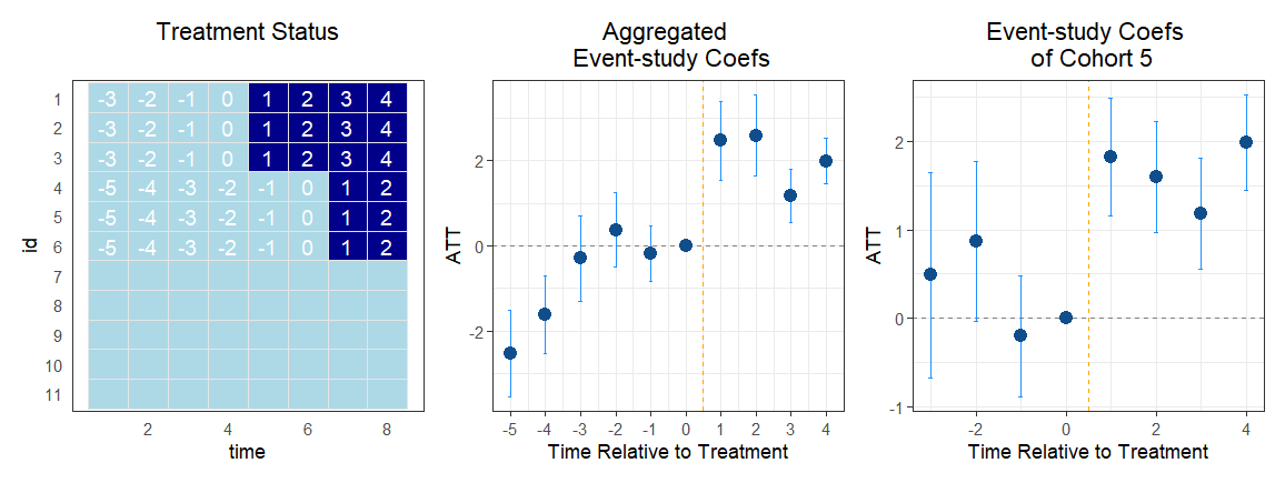
Figure 1: Challenges to Robust Inference: a Toy Example

Notes: The data are from a simulation with two treated cohorts, $\mathcal{G}_{5}$ and $\mathcal{G}_{7}$, and a never-treated cohort, $\mathcal{G}_{\infty}$. The plots show coefficients from the CS-NYT estimator. The left panel illustrates the treatment adoption status and relative periods for each observation. The center panel displays the event-study coefficients aggregated by relative period. The right panel displays the event-study coefficients for cohort $\mathcal{G}_{5}$.

To address these two challenges in robust inference under staggered adoption, I propose a cohort-anchored robust inference framework, building on the work of RR (rambachan2023more). The primary difference from RR (rambachan2023more) is that my framework bases inference on cohort-period level coefficients rather than on aggregated event-study coefficients. To address the dynamic control group issue, I introduce the concept of the block bias. Each block bias is defined at the cohort-period level and compares a treated cohort in a given period to its initial control group—the units that are untreated when this cohort first adopts treatment—relative to a reference period (or set of reference periods). Conceptually, this comparison operates within a block-adoption structure formed by the cohort and its initial control group—hence the term “block bias.” Because a treated cohort’s initial control group does not vary over time, its block biases are “anchored” to this control group and thus have a consistent interpretation in both pre- and post-treatment periods, capturing the PT violation of the treated cohort with respect to this fixed control group.

The block bias concept enables robust inference through a bias decomposition that links block biases to estimators’ biases at the cohort-period level. Formally, I define the overall bias in any post-treatment cohort-period cell as the difference between the expected value of the estimated average treatment effect and the true average treatment effect. For both the imputation and CS-NYT estimators, this overall bias can be written as a linear combination of that cohort’s own block bias and the block biases of later-treated cohorts that have begun treatment by that period. Denoting the stacked cohort-period overall biases by $\vec{\delta}$ and the stacked block biases by $\vec{\Delta}$, this decomposition implies an invertible linear mapping between them: $\vec{\delta}=\mathbf{W}\vec{\Delta}$. Appendix LABEL:sec:appendix_bias_decompose_toy provides the explicit bias decomposition for the toy example discussed previously.

In each post-treatment cohort-period cell, what can be estimated is the sum of the true treatment effect and the overall bias; neither component is separately identified. The rationale for robust inference is to impose a restriction set on the possible values of the post-treatment overall bias and, under this restriction, set-identify the true effect. This restriction set bounds the post-treatment overall bias using a benchmark learned from pre-treatment periods. Ideally, this benchmark should have the same interpretation as the overall bias in post-treatment periods. However, for the imputation estimator and the CS-NYT estimator, such benchmarks for the overall bias do not exist because the control group underlying the definition of overall bias can vary over time as discussed above.

Unlike the overall bias, block biases are defined consistently in pre- and post-treatment periods; consequently, for each cohort, observable pre-treatment block biases provide valid benchmarks for their unobservable post-treatment counterparts. The cohort-anchored robust inference framework therefore imposes restrictions on cohort-period level block biases, requiring that for each cohort, the potential block bias in post-treatment periods should not differ dramatically from the observed block bias in its pre-treatment periods. Consistent with RR (rambachan2023more), these restriction sets on block biases are specified to take the form of a single polyhedron or a union of polyhedra. Using the invertible linear mapping $\vec{\delta}=\mathbf{W}\vec{\Delta}$, the framework then translates the restriction set on the block biases into a corresponding restriction set on the overall biases. Finally, it feeds these translated restriction sets into the robust inference algorithm in RR (rambachan2023more), such as the hybrid method developed by andrews2023inference, to construct a confidence set for the average treatment effects.

The restriction sets from RR (rambachan2023more) carry over seamlessly to the cohort-anchored framework, where they become more transparent and interpretable when applied to block biases rather than to aggregated estimates. This paper focuses on two such restrictions: Relative Magnitudes (RM) and Second Differences (SD). The RM restriction bounds post-treatment changes in a cohort’s block bias between consecutive periods by a benchmark learned from pre-treatment trends. I consider both a computationally simple global benchmark, based on the maximum pre-treatment change across all cohorts, and a more theoretically sound (but computationally intensive) cohort-specific benchmark based on each cohort’s own pre-trends. The SD restriction, which is well-suited for linear pre-trends, bounds the change in the slope of the block bias path and is computationally simple as it forms a single polyhedron.

I use two simulated examples with heterogeneous pre-trends to compare my cohort-anchored framework to the robust inference framework that relies on aggregated event-study coefficients (hereafter the aggregated framework). First, in a simulation illustrating the RM restriction where one cohort has an oscillating pre-trend, the cohort-anchored framework yields markedly narrower confidence sets. This occurs because the aggregated framework adopts an overly conservative benchmark dictated by the cohort with the substantial pre-trend. Second, in a simulation illustrating the SD restriction where one cohort has a linear pre-trend, the cohort-anchored framework produces better-centered confidence sets. The aggregated framework, by contrast, uses an averaged pre-treatment slope ill-suited for any individual cohort, leading to sets centered away from the true effect. In both scenarios, the cohort-anchored approach provides more credible inference by properly accounting for cohort-level heterogeneity.

I revisit the empirical application from callaway2021-did on the effect of minimum-wage increases on teen employment, a setting with heterogeneous cohort-specific linear pre-trends that can mislead the robust inference based on aggregated coefficients. The advantages of the cohort-anchored framework are starkest under the SD restriction. While the aggregated framework produces a confidence set centered at zero, the cohort-anchored framework’s set remains centered well below zero. This demonstrates that the negative employment effect is robust to cohort-specific linear trend violations, a conclusion obscured by the aggregated framework.

Compared with robust inference based on aggregated event–study coefficients à la RR (rambachan2023more), the proposed cohort-anchored framework resolves the problems of dynamic treated composition and dynamic control group in staggered adoption settings, imposes more transparent and interpretable restriction sets, and yields better-centered confidence sets. The approach is particularly useful when there are multiple cohorts, each large enough to deliver reasonably precise cohort–period estimates, and when violations of PT differ meaningfully across cohorts.

These gains come with trade-offs. Computation can be heavier when the restriction set is a union of polyhedra because inference must be carried out across multiple benchmark configurations. Second, cohort–period estimates typically exhibit higher statistical uncertainty than aggregated coefficients, which can widen confidence sets. Finally, aggregation tends to smooth volatility in the pre-treatment series; under a fixed sensitivity parameter, the pre-treatment benchmark used by the cohort-anchored framework can sometimes be larger in magnitude than the benchmark obtained from aggregated estimates, increasing identification uncertainty and further widening confidence sets. I do not view these trade-offs as “cons” of the method; they are the price of conducting robust inference in a more transparent and interpretable way. However, in practice, although the proposed framework has many advantages, researchers may face settings with many cohorts of small size—so that cohort–period coefficients have high statistical uncertainty—in which case robust inference based on aggregated coefficients may still be preferred.

The contribution of this paper is twofold. In addition to the proposed cohort-anchored robust inference framework, the bias decomposition itself is of independent interest. While a variant of this property is first documented in aguilar2025comparative, I derive it for the imputation estimator from a different perspective. My derivation leverages the equivalence between the imputation estimator and a sequential imputation procedure, as shown in arkhangelsky2024sequential. Furthermore, the pre-treatment block bias provides a way to visualize pre-treatment coefficients for the imputation estimator that are directly comparable to their post-treatment counterparts, addressing recent discussions about the asymmetric construction and interpretation of pre- versus post-treatment coefficients in event studies (Roth2024interpret; li2025benchmarking).

The remainder of the paper proceeds as follows. Section 2 derives the bias decompositions for the imputation estimator and the CS-NYT estimator. Section LABEL:sec:inference_framework then formally lays out my robust inference framework and details how restrictions are placed on block biases. In Section LABEL:sec:illustrative_example, I use two simulated examples to illustrate the practical implementation of my framework. Section LABEL:sec:empirical_example applies the framework to the empirical application of callaway2021-did. Section LABEL:sec:conclusion concludes. All proofs appear in the Appendix. Table LABEL:tab:notation lists all notation.

2. Bias Decomposition

This section develops the bias decomposition for the imputation and CS-NYT estimators, two widely used and representative HTE-robust methods. I begin by reviewing these estimators, then formally define the concepts of block bias and overall bias, and show that the overall bias in any post-treatment cohort–period cell can be expressed as a linear combination of block biases. Next, I provide intuition for this decomposition, and finally, I discuss the estimation of block bias in pre-treatment periods and its implications for interpreting pre- and post-treatment coefficients in event studies.

2.1 Setup

I consider a DiD design with staggered treatment adoption. I observe a panel of $N$ units over $T$ time periods. Units are classified into $G$ treated cohorts, $\mathcal{G}_{g}$ for $g\in\{1,\ldots,G\}$, and a never-treated cohort $\mathcal{G}_{\infty}$. The treated cohort $\mathcal{G}_{g}$ starts to be treated in period $t_{g}$, and the number of units in each cohort is denoted by $N_{g}$ (and $N_{\infty}$ for the never-treated group). Without loss of generality, assume $1<t_{1}<\cdots<t_{G}\leq T$. The treatment status for a unit $i\in\mathcal{G}_{g}$ is thus $D_{it}=\mathbf{1}\{t\geq t_{g}\}$, while for never-treated units, $D_{it}=0$ for all $t$. The observed outcome is $Y_{it}=D_{it}Y_{it}(1)+(1-D_{it})Y_{it}(0)$, where $Y_{it}(1)$ and $Y_{it}(0)$ are the potential outcomes under treatment and control, respectively. I use $t\in\{1,\ldots,T\}$ to denote the calendar period and $s$ to denote the period relative to the treatment date. For a given cohort $\mathcal{G}_{g}$, $s=1$ corresponds to the first post-treatment period ($t=t_{g}$), while $s=0$ corresponds to the last pre-treatment period ($t=t_{g}-1$).

Throughout this paper, I assume a balanced panel in a staggered adoption setting without covariates. My analysis therefore focuses on the unconditional, rather than the conditional, PT assumption. I also assume the existence of a never-treated cohort.

Assumption 1 (Model Setup).

2. Staggered Adoption: $1<t_{1}<\cdots<t_{G}\leq T$.

3. Never-Treated Cohort: The set of never-treated units is non-empty, i.e., $|\mathcal{G}_{\infty}|=N_{\infty}>0$.

4. Balanced Panel: The data matrix $\{Y_{it}\}$ is complete for all units $i\in\bigcup_{g=1}^{G}\mathcal{G}_{g}\cup\mathcal{G}_{\infty}$ and all time periods $t\in\{1,\dots,T\}$.

The potential outcome notation, $Y_{it}(0)$, is a simplification that implicitly bundles some identifying assumptions as one unit’s potential outcome could depend on the entire vector of treatment assignments across all units and time. I therefore formally separate the assumptions required to simplify this general case. They can be understood as two facets of the no interference principle: one that restricts interference across units (SUTVA) and another that restricts interference across time (no anticipation).

Assumption 2 (No Interference).

2. Across Units (SUTVA): The potential outcomes for any unit $i$ do not depend on the treatment status of any other unit $j\neq i$. This rules out spillover effects across units.

3. Across Time (No Anticipation): The potential outcomes for any unit $i$ in period $t$ do not depend on its treatment status in future periods.

Imputation Estimator

The imputation estimator, proposed by borusyak2024revisiting and liu2024practical, is a popular approach for DiD designs. The procedure begins by estimating unit and time fixed effects, $(\hat{\alpha}_{i},\hat{\xi}_{t})$, from a two-way fixed effects model fitted using only the untreated observations in the panel. These estimates are then used to impute the counterfactual outcome for each treated observation: $\hat{Y}_{i,t_{g}+s-1}(0)=\hat{\alpha}_{i}+\hat{\xi}_{t_{g}+s-1}$. The estimated average treatment effect for cohort $\mathcal{G}_{g}$ at relative period $s$ is the average difference between the observed and imputed outcomes: ^τ_G_g,s^Imp = 1Ng∑_i∈G_g [ Y_i,t_g+s-1 - ^Y_i,t_g+s-1(0) ]. This estimator has several attractive properties that make it a popular alternative to traditional TWFE regression. Most importantly, because the fixed effects are estimated using only untreated observations, the resulting treatment effect estimates are robust to HTE and avoid the negative weighting problems that can bias standard TWFE estimators in staggered designs. Furthermore, borusyak2024revisiting show that the imputation estimator is the most efficient linear unbiased estimator under the assumption of homoskedastic and serially uncorrelated errors (spherical errors).

The CS-NYT Estimator

callaway2021-did provides alternative estimators for $\tau_{\mathcal{G}_{g},s}$. One of them compares the change in the average outcome for a treated cohort $\mathcal{G}_{g}$ to the corresponding change for a control group consisting of not-yet-treated units, denoted $\mathcal{C}_{g,s}=\left(\cup_{k:t_{k}>t}\mathcal{G}_{k}\right)\cup\mathcal{G}_{\infty}$, where $t=t_{g}+s-1$. A key feature of this method is that the control group $\mathcal{C}_{g,s}$ is defined contemporaneously and therefore shrinks as later cohorts receive treatment. The initial control group for cohort $\mathcal{G}_{g}$ is the set of not-yet-treated units at its first period of treatment ($s=1$), which I denote as $\mathcal{C}_{g,1}$.

The estimator compares the change between the last pre-treatment period, $t_{g}-1$, and a given post-treatment period, $t_{g}+s-1$. The estimated average treatment effect for cohort $\mathcal{G}_{g}$ at relative period $s$ is ^τ_G_g,s^CS-NYT = 1Ng∑_i∈G_g(Y_i,t_g+s-1-Y_i,t_g-1) - 1NCg,s∑_i∈C_g,s(Y_i,t_g+s-1-Y_i,t_g-1), where the time-varying control group $\mathcal{C}_{g,s}$ is defined on each relative post-treatment period $s\geq 1$. callaway2021-did also discuss extensions that incorporate covariates using outcome regression, inverse probability weighting, and doubly robust techniques.

Other HTE-Robust Estimators

The landscape of HTE-robust DiD estimators also includes several other important methods. For instance, the CS-NT estimator in callaway2021-did that uses the never treated as controls and the regression-based estimator of sun2021-event both identify treatment effects using a fixed, never-treated control group. Another key approach, the $\text{DID}_{l}$ estimator of de2024difference, is closely related to the CS-NYT estimator I focus on.

In the setting of a balanced panel with staggered adoption and no covariates, the estimator of sun2021-event is equivalent to the CS-NT estimator. My framework’s core theoretical results can therefore be readily applied to this wider class of estimators. For methods that use a uniform control group, the bias decomposition becomes trivial, as adjustment for the varying control group is no longer needed.

2.2 Overall bias and Block Bias

I now formally define the overall bias ($\delta_{\mathcal{G}_{g},s}$) and the block bias ($\Delta_{\mathcal{G}_{g},s}$). Both concepts are defined on each cohort-period cell $(g,s)$ and form the foundation of the bias decomposition and robust inference framework that follows.

Overall bias

For the imputation estimator, I define the overall bias for cohort $\mathcal{G}_{g}$ in a post-treatment period $s\geq 1$, denoted $\delta^{\text{Imp}}_{\mathcal{G}_{g},s}$, as the difference between the expectation of the estimated treatment effect and the true treatment effect in that cohort-period cell. As the derivation below shows, this simplifies to the difference between the true and the imputed counterfactuals:

$$\begin{split}\delta^{\text{Imp}}_{\mathcal{G}_{g},s}&\equiv\mathbb{E}[\hat{\tau}_{\mathcal{G}_{g},s}^{\text{Imp}}]-\tau_{\mathcal{G}_{g},s}\\ &=\left(\mathbb{E}[Y_{i,t_{g}+s-1}\mid i\in\mathcal{G}_{g}]-\mathbb{E}[\hat{Y}_{i,t_{g}+s-1}(0)\mid i\in\mathcal{G}_{g}]\right)\\ &\quad-\left(\mathbb{E}[Y_{i,t_{g}+s-1}\mid i\in\mathcal{G}_{g}]-\mathbb{E}[Y_{i,t_{g}+s-1}(0)\mid i\in\mathcal{G}_{g}]\right)\\ &=\mathbb{E}[Y_{i,t_{g}+s-1}(0)\mid i\in\mathcal{G}_{g}]-\mathbb{E}[\hat{Y}_{i,t_{g}+s-1}(0)\mid i\in\mathcal{G}_{g}].\end{split}$$ (Overall-Bias-Imp)

The overall bias for the CS-NYT estimator can be defined analogously in post-treatment periods:

$$\begin{split}\delta^{\text{CS-NYT}}_{\mathcal{G}_{g},s}&\equiv\mathbb{E}[\hat{\tau}_{\mathcal{G}_{g},s}^{\text{CS-NYT}}]-\tau_{\mathcal{G}_{g},s}\\ &=\left(\mathbb{E}[Y_{i,t_{g}+s-1}\mid i\in\mathcal{G}_{g}]-\mathbb{E}[Y_{i,t_{g}-1}(0)\mid i\in\mathcal{G}_{g}]\right)-\left(\mathbb{E}[Y_{i,t_{g}+s-1}(0)\mid i\in\mathcal{C}_{g,s}]-\mathbb{E}[Y_{i,t_{g}-1}(0)\mid i\in\mathcal{C}_{g,s}]\right)\\ &\quad-\left(\mathbb{E}[Y_{i,t_{g}+s-1}\mid i\in\mathcal{G}_{g}]-\mathbb{E}[Y_{i,t_{g}+s-1}(0)\mid i\in\mathcal{G}_{g}]\right)\\ &=\left(\mathbb{E}[Y_{i,t_{g}+s-1}(0)\mid i\in\mathcal{G}_{g}]-\mathbb{E}[Y_{i,t_{g}-1}(0)\mid i\in\mathcal{G}_{g}]\right)\\ &\quad-\left(\mathbb{E}[Y_{i,t_{g}+s-1}(0)\mid i\in\mathcal{C}_{g,s}]-\mathbb{E}[Y_{i,t_{g}-1}(0)\mid i\in\mathcal{C}_{g,s}]\right).\end{split}$$ (Overall-Bias-CS-NYT)

Note that $Y_{i,t_{g}+s-1}(0)=Y_{i,t_{g}+s-1}$ for $i\in\mathcal{C}_{g,s}$ and $Y_{i,t_{g}-1}(0)=Y_{i,t_{g}-1}$ for $i\in\mathcal{C}_{g,s}\bigcup\mathcal{G}_{g}$. The bias term $\delta^{\text{CS-NYT}}_{\mathcal{G}_{g},s}$ therefore represents the difference between two trends from the reference period $t_{g}-1$ to the post-treatment period $t_{g}+s-1$: (1) the counterfactual trend for cohort $\mathcal{G}_{g}$ under no treatment, and (2) the observed trend for the not-yet-treated control group, $\mathcal{C}_{g,s}$. The condition that this bias term is zero, $\delta^{\text{CS-NYT}}_{\mathcal{G}_{g},s}=0$, is precisely the PT assumption required for the unbiased estimation of $\tau_{\mathcal{G}_{g},s}$.

The overall bias terms, $\delta^{\text{Imp}}_{\mathcal{G}_{g},s}$ and $\delta^{\text{CS-NYT}}_{\mathcal{G}_{g},s}$, represent the bias in the estimated treatment effect for a given post-treatment cohort-period cell $(g,s)$. The goal of robust inference is to use observable pre-trends to form a restriction set on these unobservable post-treatment biases. For the restriction to be interpretable and credible, the benchmark derived from pre-trends should have the same interpretation as the post-treatment biases. However, the overall bias is ill-suited for this task. Specifically, one cannot find a measure of the pre-trend that best mirrors the overall bias in post-treatment periods. For the imputation estimator, the overall bias lacks a symmetrically defined pre-treatment analog. For the CS-NYT estimator, the control group’s composition changes in post-treatment periods, meaning no single pre-treatment comparison can serve as a consistent benchmark for all post-treatment periods. These challenges motivate my introduction of the block bias.

Block Bias

The block bias, $\Delta_{\mathcal{G}_{g},s}$, captures the violation of PT for a cohort $\mathcal{G}_{g}$ relative to its fixed, initial control group, $\mathcal{C}_{g,1}=\left(\bigcup_{k:t_{k}>t_{g}}\mathcal{G}_{k}\right)\cup\mathcal{G}_{\infty}$. This group consists of all units not-yet-treated at the moment cohort $\mathcal{G}_{g}$ first receives treatment ($s=1$). Because this comparison group is, by definition, fixed for all relative periods $s$, the block bias provides a consistent measure of the trend difference between $\mathcal{G}_{g}$ and $\mathcal{C}_{g,1}$ in both pre- and post-treatment periods. I use the term “block” because this comparison operates within a classic block-adoption structure formed by $\mathcal{G}_{g}$ and its initial control group $\mathcal{C}_{g,1}$.

The exact definition of the block bias depends on the estimator. For the imputation estimator, the block bias is defined as:

$$\begin{split}\Delta_{\mathcal{G}_{g},s}^{\text{Imp}}&=\left(\mathbb{E}[Y_{i,t_{g}+s-1}(0)\mid i\in\mathcal{G}_{g}]-\mathbb{E}[\bar{Y}_{i,\text{pre}_{g}}(0)\mid i\in\mathcal{G}_{g}]\right)\\ &\quad-\left(\mathbb{E}[Y_{i,t_{g}+s-1}(0)\mid i\in\mathcal{C}_{g,1}]-\mathbb{E}[\bar{Y}_{i,\text{pre}_{g}}(0)\mid i\in\mathcal{C}_{g,1}]\right),\end{split}$$ (Block-Bias-Imp)

where $\text{pre}_{g}=\{1,\dots,t_{g}-1\}$ denotes the set of pre-treatment periods for cohort $\mathcal{G}_{g}$, and $\bar{Y}_{i,\text{pre}_{g}}(0)=\frac{1}{t_{g}-1}\sum_{t\in\text{pre}_{g}}Y_{it}(0)$ is the average potential outcome for unit $i$ over those periods. By definition, no units in cohort $\mathcal{G}_{g}$ or its initial control group $\mathcal{C}_{g,1}$ are treated during the $\text{pre}_{g}$ window. Therefore, their potential outcomes are equal to their observed outcomes during periods $\text{pre}_{g}$ (i.e., $Y_{i,t}(0)=Y_{i,t}$ for $i\in\mathcal{G}_{g}\bigcup\mathcal{C}_{g,1}$ and $t\in\text{pre}_{g}$).

The term $\Delta_{\mathcal{G}_{g},s}^{\text{Imp}}$ takes a classic DiD-like structure. The first component, $\mathbb{E}[Y_{i,t_{g}+s-1}(0)\mid i\in\mathcal{G}_{g}]-\mathbb{E}[\bar{Y}_{i,\text{pre}_{g}}(0)\mid i\in\mathcal{G}_{g}]$ represents the trend in cohort $\mathcal{G}_{g}$’s potential outcome, measuring its value in a given period relative to the average over all its pre-treatment periods. The block bias, $\Delta_{\mathcal{G}_{g},s}^{\text{Imp}}$, is the difference between this trend for cohort $\mathcal{G}_{g}$ and the corresponding trend for its initial control group, $\mathcal{C}_{g,1}$. A key feature of this definition is that the block bias is directly observable in all pre-treatment periods ($s\leq 0$), while in post-treatment periods ($s>0$) it becomes unobservable. This unobservability arises because not only the potential outcomes for the treated cohort $\mathcal{G}_{g}$ are unknown by definition, but also the potential outcomes for some units in the initial control group $\mathcal{C}_{g,1}$ may become unobservable once they themselves are treated at later dates.

Crucially, the definition and interpretation of the block bias remain identical across all pre- and post-treatment periods. It always compares the trend of the treated cohort with the trend of its anchored initial control group. This consistency allows observable pre-treatment block biases to serve as valid benchmarks for unobservable post-treatment block biases.

The block bias for the CS-NYT estimator takes a similar form, but uses the last pre-treatment period of the target cohort, $t_{g}-1$, as the reference period. Formally, it is defined as:

$$\begin{split}\Delta_{\mathcal{G}_{g},s}^{\text{CS-NYT}}&=\left(\mathbb{E}[Y_{i,t_{g}+s-1}(0)\mid i\in\mathcal{G}_{g}]-\mathbb{E}[Y_{i,t_{g}-1}(0)\mid i\in\mathcal{G}_{g}]\right)\\ &\quad-\left(\mathbb{E}[Y_{i,t_{g}+s-1}(0)\mid i\in\mathcal{C}_{g,1}]-\mathbb{E}[Y_{i,t_{g}-1}(0)\mid i\in\mathcal{C}_{g,1}]\right).\end{split}$$ (Block-Bias-CS-NYT)

This definition closely resembles that of the overall bias in Equation (Overall-Bias-CS-NYT). The critical difference is that the block bias compares cohort $\mathcal{G}_{g}$ to its fixed initial control group, $\mathcal{C}_{g,1}$, whereas the overall bias uses the time-varying not-yet-treated control group, $\mathcal{C}_{g,s}$. The same as the imputation estimator, this definition allows the observable pre-treatment estimates of $\Delta_{\mathcal{G}_{g},s}^{\text{CS-NYT}}$ to serve as a valid benchmark for its unobservable post-treatment counterparts.

For any treated cohort, the overall bias and block bias are equivalent in the first post-treatment period ($s=1$), $\delta_{\mathcal{G}_{g},1}=\Delta_{\mathcal{G}_{g},1}$. For the CS-NYT estimator, this result is straightforward. At the first post-treatment period, the not-yet-treated control group is, by definition, identical to the initial control group. For the imputation estimator, this equality follows directly from the lemma below.

Lemma 1.

For any treated unit $i\in\mathcal{G}_{g}$ in its first post-treatment period $t_{g}$, the counterfactual imputed by the imputation estimator, $\hat{Y}^{\text{Imp}}_{i,t_{g}}(0)$, is algebraically equivalent to a simple block-DiD expression:

$$\hat{Y}_{i,t_{g}}^{\text{Imp}}(0)=\overline{Y}_{i,\text{pre}_{g}}+\bigl(\overline{Y}_{\mathcal{C}_{g,1},t_{g}}-\overline{Y}_{\mathcal{C}_{g,1},\text{pre}_{g}}\bigr),$$

where $\mathcal{C}_{g,1}$ is the initial control group, $\overline{Y}_{\mathcal{C}_{g,1},t_{g}}$ is the average outcome for this group at time $t_{g}$, and $\overline{Y}_{\mathcal{C}_{g,1},\text{pre}_{g}}$ is this group’s average outcome over cohort $\mathcal{G}_{g}$’s pre-treatment periods.

Proof of Lemma 1 is provided in the Appendix LABEL:proof:initial_period_equivalence.

This lemma establishes an exact algebraic identity for the imputed counterfactual in the first post-treatment period. Taking the expectation of the expression in Lemma 1 implies that the overall bias, $\delta^{\text{Imp}}_{\mathcal{G}_{g},1}$, is equivalent to the block bias, $\Delta^{\text{Imp}}_{\mathcal{G}_{g},1}$, for every treated cohort. This equivalence provides a crucial link between the full, staggered panel and the simpler block structure consisting of cohort $\mathcal{G}_{g}$ and its initial control group, furnishing the first step for the bias decomposition that follows.

2.3 The Bias Decomposition

For relative periods beyond the first post-treatment period ($s>1$), the overall bias is no longer identical to the block bias. For both the imputation and the CS-NYT estimators, the control group for an early-adopting cohort changes over time as some cohorts in the initial control group receive treatment later. This dynamic produces a recursive structure where the overall bias of one cohort depends on the block biases of those treated after it.

The following proposition formalizes this relationship for the imputation estimator, decomposing the overall bias for any cohort-period cell into its own block bias plus a linear combination of the block biases of later-adopting cohorts. This result is a variant of the Corollary 1 in aguilar2025comparative, though my formulation and proof—which leverages the sequential nature of the imputation estimator—are distinct.

Proposition 2.1 (Bias Decomposition for the Imputation Estimator).

Let $t=t_{g}+s-1$ be the calendar time corresponding to post-treatment period $s\geq 1$ for cohort $\mathcal{G}_{g}$. Then the overall bias $\delta^{\text{Imp}}_{\mathcal{G}_{g},s}$ satisfies

$$\delta^{\text{Imp}}_{\mathcal{G}_{g},s}=\Delta^{\text{Imp}}_{\mathcal{G}_{g},s}+\sum_{k\in\mathcal{K}_{g}(t)}\left(\frac{N_{k}}{\sum_{j=k}^{G}N_{j}+N_{\infty}}\right)\Delta^{\text{Imp}}_{\mathcal{G}_{k},s_{k}(t)}$$

where the set of later-treated cohorts that contributes to $\delta^{\text{Imp}}_{\mathcal{G}_{g},s}$ is $\mathcal{K}_{g}(t)=\bigl\{k\,\big|\,t_{g}<t_{k}\leq t\bigr\}$ and the relative period for such a cohort $\mathcal{G}_{k}$ is $s_{k}(t)=t-(t_{k}-1)$.

Proof. See Appendix LABEL:proof:bias-decompose-impute.

Proposition 2.1 shows that the overall bias from the imputation estimator for cohort $\mathcal{G}_{g}$ at a post-treatment period $s$, $\delta^{\text{Imp}}_{\mathcal{G}_{g},s}$, equals its own block bias, $\Delta^{\text{Imp}}_{\mathcal{G}_{g},s}$, plus a weighted sum of block biases from a specific set of later-adopting cohorts. These cohorts, which I term adjustment cohorts, are those that begin treatment after $\mathcal{G}_{g}$ and no later than calendar time $t=t_{g}+s-1$, denoted by the set $\mathcal{K}_{g}(t)=\bigl\{k\,\big|\,t_{g}<t_{k}\leq t\bigr\}$. The weight assigned to each adjustment cohort $\mathcal{G}_{k}$ depends on its size, $N_{k}$, relative to the total size of $\mathcal{G}_{k}$ and $\mathcal{G}_{k}$’s initial control group, $\mathcal{C}_{k,1}$, which is $\frac{N_{k}}{N_{k}+N_{\mathcal{C}_{k,1}}}=\frac{N_{k}}{\sum_{j=k}^{G}N_{j}+N_{\infty}}$. Finally, the relative period for each adjustment cohort, $s_{k}(t)=t-t_{k}+1$, ensures its block bias is evaluated at the same calendar time $t$ as the overall bias it adjusts.

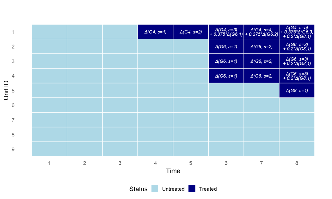
Figure 2: Bias Decomposition of the Imputation Estimator

Notes: The figure illustrates the bias decomposition from Proposition 2.1 using an example with three treated cohorts ($\mathcal{G}_{4}$ at $t=4$, $\mathcal{G}_{6}$ at $t=6$, $\mathcal{G}_{8}$ at $t=8$) and a never-treated group (units 6-9). Each treated (dark blue) cell shows how the overall bias ($\delta$) for a given cohort-period is the sum of the cohort’s own block bias ($\Delta$) and the weighted block biases of later-adopting cohorts.

To illustrate the bias-decomposition formula from Proposition 2.1, Figure 2 presents an illustrative panel with three treated cohorts and one never-treated group. Cohort $\mathcal{G}_{4}$ (unit 1) is treated at $t=4$, Cohort $\mathcal{G}_{6}$ (units 2–4) at $t=6$, and Cohort $\mathcal{G}_{8}$ (unit 5) at $t=8$. Each dark-blue cell denotes a treated observation, and the expression inside displays how the overall bias, $\delta^{\text{Imp}}$, for that observation’s cohort, is decomposed into its constituent block biases, $\Delta^{\text{Imp}}$.

In each cohort’s first post-treatment period, as Lemma 1 suggests, the overall bias equals the cohort’s own block bias. In later periods, the overall bias for early adopters becomes the sum of their own block bias and the block biases from their adjustment cohorts. For instance, at $t=6$, Cohort $\mathcal{G}_{6}$ begins to receive treatment, and the overall bias for Cohort $\mathcal{G}_{4}$ becomes $\delta^{\text{Imp}}_{\mathcal{G}_{4},s=3}=\Delta^{\text{Imp}}_{\mathcal{G}_{4},s=3}+0.375\,\Delta^{\text{Imp}}_{\mathcal{G}_{6},s=1}$. The weight of 0.375 is determined by Cohort $\mathcal{G}_{6}$’s size ($N_{6}=3$) relative to the total size of Cohort $\mathcal{G}_{6}$ and its initial control group, calculated as $0.375=\frac{N_{6}}{N_{6}+N_{8}+N_{\infty}}=\frac{3}{3+1+4}$. Similarly, when $\mathcal{G}_{8}$ is treated at $t=8$, its block bias, $\Delta^{\text{Imp}}_{\mathcal{G}_{8},s=1}$, contributes to the overall bias of $\mathcal{G}_{4}$ ($\delta^{\text{Imp}}_{\mathcal{G}_{4},s=5}$) and $\mathcal{G}_{6}$ ($\delta^{\text{Imp}}_{\mathcal{G}_{6},s=3}$) with a weight of $\frac{N_{8}}{N_{8}+N_{\infty}}=\frac{1}{1+4}=0.2$.

The bias decomposition for the CS-NYT estimator takes a slightly different form, as stated in Proposition 2.2. This result is also a variant to the Corollary 3 in aguilar2025comparative, albeit with a different formulation and proof.

Proposition 2.2 (Bias Decomposition for the CS-NYT Estimator).

Let $t=t_{g}+s-1$ be the calendar time corresponding to post-treatment period $s\geq 1$ for cohort $\mathcal{G}_{g}$. Then the overall bias $\delta^{\text{CS-NYT}}_{\mathcal{G}_{g},s}$ satisfies

$$\delta^{\text{CS-NYT}}_{\mathcal{G}_{g},s}=\Delta^{\text{CS-NYT}}_{\mathcal{G}_{g},s}+\sum_{k\in\mathcal{K}_{g}(t)}\left(\frac{N_{k}}{\sum_{j=k}^{G}N_{j}+N_{\infty}}\right)(\Delta^{\text{CS-NYT}}_{\mathcal{G}_{k},s_{k}(t)}-\Delta^{\text{CS-NYT}}_{\mathcal{G}_{k},s_{k}(t_{g}-1)})$$

where the set of adjustment cohorts is $\mathcal{K}_{g}(t)=\{k\mid t_{g}<t_{k}\leq t\}$, and the relative periods for cohort $\mathcal{G}_{k}$ are $s_{k}(t)=t-t_{k}+1$ and $s_{k}(t_{g}-1)=(t_{g}-1)-(t_{k}-1)=t_{g}-t_{k}$.

Proof. See Appendix LABEL:proof:bias-decompose-CS.

While the definitions of the bias terms ($\delta^{\text{CS-NYT}}$ and $\Delta^{\text{CS-NYT}}$) differ from the imputation estimator, the weights on the adjustment terms, $\frac{N_{k}}{\sum_{j=k}^{G}N_{j}+N_{\infty}}$, are identical. The distinction lies in the structure of the adjustment term. For the imputation estimator, the adjustment is a single block bias, $\Delta^{\text{Imp}}_{\mathcal{G}_{k},s_{k}}$. For the CS-NYT estimator, the adjustment term from $\mathcal{G}_{k}$ is the difference between two of its block biases: $\Delta^{\text{CS-NYT}}_{\mathcal{G}_{k},s_{k}(t)}-\Delta^{\text{CS-NYT}}_{\mathcal{G}_{k},s_{k}(t_{g}-1)}$. This structure arises because the block biases of $\mathcal{G}_{g}$ and $\mathcal{G}_{k}$ are measured with respect to different reference periods. The block bias for cohort $\mathcal{G}_{g}$ is defined relative to its reference period ($t_{g}-1$), while the block bias for a later cohort $\mathcal{G}_{k}$ is defined relative to $\mathcal{G}_{k}$’s reference period ($t_{k}-1$). To make them comparable, the adjustment term for cohort $\mathcal{G}_{k}$ must be re-calibrated to cohort $\mathcal{G}_{g}$’s baseline. The term $\Delta^{\text{CS-NYT}}_{\mathcal{G}_{k},s_{k}(t_{g}-1)}$ serves as this baseline correction. Since $s_{k}(t_{g}-1)=t_{g}-t_{k}<0$, this correction term is simply a pre-treatment block bias of $\mathcal{G}_{k}$. Subtracting this term isolates the component of the block bias from $\mathcal{G}_{k}$ that is properly aligned with $\mathcal{G}_{g}$’s block bias.

A key component of the bias decompositions in Propositions 2.1 and 2.2 is the weights placed on the adjustment cohort, $\mathcal{K}_{g}(t)$. The form, $w_{k}=\frac{N_{k}}{\sum_{j=k}^{G}N_{j}+N_{\infty}}$, implies that in $\mathcal{K}_{g}(t)$, (i) cohorts with larger population sizes $N_{k}$ receive larger weights; and (ii) with fixed cohort sizes, later-treated cohorts (larger $k$) in $\mathcal{K}_{g}(t)$ receive larger weights, since $\sum_{j=k}^{G}N_{j}$ decreases in $k$. The identical weights in both propositions highlight a similarity between the two estimators. Although they take different forms and have different implementations, both the imputation estimator and the CS-NYT estimator compare the trend of a treated cohort to that of its not-yet-treated control group. The primary distinction lies in how they use pre-treatment information: the imputation estimator uses the average of outcomes across all pre-treatment periods as the reference, while the CS-NYT estimator uses only the last pre-treatment period as the reference period. chen2025efficient provides a detailed discussion on the differences between these two estimators from this perspective.

Both propositions show that the overall bias of any post-treatment cohort-period cell can be expressed as a linear combination of block biases. For notational simplicity, I extend this relationship across all periods by defining the overall bias in pre-treatment periods to be equal to the block bias in the same periods. With this convention in place, the entire system of biases can be written compactly in matrix form. The stacked vectors of overall biases ($\vec{\delta}$) and block biases ($\vec{\Delta}$) are then related by the invertible linear mapping: $\vec{\delta}=\mathbf{W}\vec{\Delta}$.

Order the cohort–period cells $(g,s)$ by increasing calendar time $t=t_{g}+s-1$ and, within each $t$, by increasing adoption time $t_{g}$. Under this stacking, the mapping matrix $\mathbf{W}$ is block diagonal for the imputation estimator and block triangular for the CS-NYT estimator across calendar times:

$$\mathbf{W}=\begin{cases}\mathrm{diag}(A_{1},\dots,A_{T}),&\text{(Imputation)}\\[6.0pt] \begin{bmatrix}A_{1}&0&\cdots&0\\ *&A_{2}&\ddots&\vdots\\ \vdots&\ddots&\ddots&0\\ *&\cdots&*&A_{T}\end{bmatrix},&\text{(CS-NYT),}\end{cases}$$

where for each $t$ the diagonal block $A_{t}$ is unit upper–triangular. Hence $\mathrm{det}(A_{t})=1$ for all $t$, and by the block–triangular determinant identity, $\mathrm{det}(\mathbf{W})=\prod_{t=1}^{T}\mathrm{det}(A_{t})=1\neq 0$. Therefore $\mathbf{W}$ is square and invertible (with $\mathbf{W}^{-1}$ block–diagonal in the imputation case and block lower–triangular in the CS-NYT case). Appendix LABEL:sec:appendix_bias_decompose_toy provides the explicit form of the $\mathbf{W}$ matrix for the CS-NYT estimator as applied to the toy example in the introduction.

2.4 Intuition of the Bias Decomposition

The intuition behind the bias decomposition for the imputation estimator becomes clear by conceptualizing it as a sequential procedure that constructs the counterfactual panel one relative period at a time. The equivalence between the imputation estimator and sequential procedures is studied by arkhangelsky2024sequential that considers a more general form with unit- or period-specific weights. My derivation of the bias decomposition follows this sequential approach, providing an alternative perspective to the direct matrix algebra used in aguilar2025comparative.

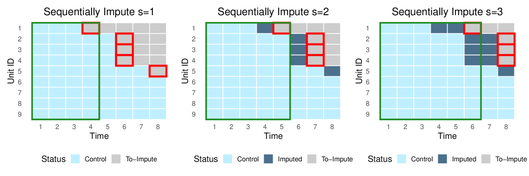
Figure 3: Sequential Procedure of the Imputation Estimator

Notes: The figure visualizes the imputation estimator as a sequential procedure that proceeds one relative period at a time. In each step (panel), the counterfactuals for the cells to be imputed (gray with red outlines) are calculated using all available control (light blue) and previously imputed (dark blue) data. This illustrates how imputations for early-adopting cohorts in later periods (e.g., unit 1 at $t=6$) depend on the imputed values of later-adopting cohorts (e.g., units 2-4 at $t=6$). The green rectangle marks the block comprising unit 1 (cohort $\mathcal{G}_{4}$) and its initial control group, which is used to construct the imputed counterfactual for unit 1 in the corresponding post-treatment period.

Figure 3 illustrates this sequential procedure with the example in Figure 2. Imagine starting with a data matrix containing only the observed outcomes of untreated cells (light blue). The procedure begins by imputing all cells corresponding to the first post-treatment period, $s=1$ (highlighted in red in the left panel). For each such cohort-period cell, the counterfactual is imputed using a block structure that consists of the cohort and its initial controls, utilizing data from the current and all prior periods (marked by the green rectangle). For example, the counterfactual for unit 1 (cohort $\mathcal{G}_{4}$) at $t=4$ is constructed as $\hat{Y}_{1,4}(0)=\bar{Y}_{1,\text{pre}_{4}}(0)+[\bar{Y}_{\mathcal{C}_{4,1},4}(0)-\bar{Y}_{\mathcal{C}_{4,1},\text{pre}_{4}}(0)]$, where $\text{pre}_{4}=\{1,2,3\}$ and the initial control group $\mathcal{C}_{4,1}$ consists of units 2 through 9. After this step, the imputed values for all $s=1$ cells fill their corresponding entries in the matrix.

The procedure continues by imputing cells for $s=2$ (middle panel), then $s=3$ (right panel), and so on. The key feature of these later rounds is that the construction of counterfactuals may rely on previously imputed values. For instance, to impute the counterfactual for unit 1 at $t=6$ (in the $s=3$ round), the procedure uses the formula: $\hat{Y}_{1,6}(0)=\bar{Y}_{1,\text{pre}_{6}}(0)+[\bar{Y}_{\mathcal{C}_{4,1},6}(0)-\bar{Y}_{\mathcal{C}_{4,1},\text{pre}_{6}}(0)]$ where $\text{pre}_{6}=\{1,2,3,4,5\}$. However, units 2, 3, and 4 are treated at this time, the calculation of $\bar{Y}_{\mathcal{C}_{4,1},6}(0)$ thus uses their imputed counterfactuals—$\hat{Y}_{2,6}(0),\hat{Y}_{3,6}(0),$ and $\hat{Y}_{4,6}(0)$—which were already imputed during the $s=1$ round. Similarly, the calculation of $\bar{Y}_{1,\text{pre}_{6}}(0)$ also uses values for unit 1 that were imputed during the earlier $s=1$ and $s=2$ rounds.

This iterative process continues over all cohort-period cells from $s=1$ to the largest post-treatment relative periods. I prove in Appendix LABEL:prop:impute-seq-impute-equivalence that this sequential procedure yields results that are numerically equivalent to the standard imputation estimator that solves for and uses all fixed effects simultaneously.

The equivalence between the imputation estimator and the sequential procedure implies that every cohort-period level imputed counterfactual can be expressed as a DiD-style comparison within the block structure formed by the cohort and its initial controls. Specifically, for any post-treatment cell $(g,s)$ at calendar time $t=t_{g}+s-1$, the average imputed counterfactual can be constructed with: ^Y_G_g, t(0) = ¯Y^*_G_g, pre_t(0) + [¯Y^*_C_g,1, t(0) - ¯Y^*_C_g,1, pre_t(0)] where the terms on the right-hand side are: (i) $\bar{Y}^{*}_{\mathcal{G}_{g},\text{pre}_{t}}(0)$ is the average untreated outcome for cohort $\mathcal{G}_{g}$ over all prior periods; (ii) $\bar{Y}^{*}_{\mathcal{C}_{g,1},t}(0)$ is the average untreated outcome for its initial control group at the current time $t$; and (iii) $\bar{Y}^{*}_{\mathcal{C}_{g,1},\text{pre}_{t}}(0)$ is the average untreated outcome for the initial control group over all prior periods. The star (${}^{*}$) signifies that these averages are taken over observed untreated outcomes or, if unavailable, over counterfactuals imputed in previous imputation rounds.

The overall bias for a post-treatment cell $(g,s)$ with calendar time $t$ is the expected difference between the true and imputed counterfactuals for cohort $\mathcal{G}_{g}$. Its finite-sample expression is: ¯Y_G_g,t(0)-^Y_G_g, t(0) = [¯Y_G_g,t(0)-¯Y^*_G_g, pre_t(0)] - [