When LLM Meets Time Series: Can LLMs Perform Multi-Step Time Series Reasoning and Inference
Abstract
The rapid advancement of Large Language Models (LLMs) has sparked growing interest in their application to time series analysis tasks. However, their ability to perform complex reasoning over temporal data application domain remains significantly underexplored. To achieve the goal, one first step is to establish a rigorous benchmark dataset for evaluation. In this work, we introduce TSAIA Benchmark, a first attempt to evaluate LLMs as time series artificial intelligence assistant. To ensure both scientific rigor and practical relevance, we surveyed over 20 academic publications and identified 33 real-world task formulations. The benchmark encompasses a broad spectrum of challenges, ranging from constraint-aware forecasting to anomaly detection with threshold calibration—tasks that require compositional reasoning and multi-step time series analysis. The question generator is designed to be dynamic and extensible, supporting continuous expansion as new datasets or task types are introduced. Given the heterogeneous nature of the tasks, we adopt task-specific success criteria and tailored inference quality metrics to ensure meaningful evaluation for each task. We apply this benchmark to assess 8 state-of-the-art LLMs under a unified evaluation protocol. Our analysis reveals limitations in current models’ ability to assemble complex time series analysis workflows, underscoring the need for specialized methodologies for adaptation towards domain-specific applications. Our benchmark is available at https://huggingface.co/datasets/Melady/TSAIA, and the code is available at https://github.com/USC-Melady/TSAIA.
1 Introduction
Large Language Models (LLMs) have demonstrated remarkable general-purpose capabilities across a range of domains, including language understanding dong2019unified , code generation jiang2024survey , and scientific reasoning taylor2022galactica . Despite their growing capabilities, large language models have not been evaluated for time series analysis, which constitutes a fundamental competency for data analysts and scientists across critical domains including energy alvarez2010energy , finance sezer2020financial , climate science mudelsee2019trend , and healthcare rathlev2007time . In practice, time series workflows in the real world are inherently complex yan2021learning ; han2021real : they demand multi-step reasoning fu2022complexity , precise numerical computation cvejoski2022future , integration of domain knowledge xue2024domain , and adherence to operational constraints wang220kv . With the advent of agent systems, there is growing interest among practitioners in developing intelligent agents capable of interpreting natural language instructions to perform time series analysis. However, given that time series understanding poses challenges even for humans, researchers are striving to establish a clear paradigm for how LLMs can effectively contribute to these complex downstream tasks. A crucial step toward empowering LLMs in time series applications is the development of rigorous benchmark datasets for comprehensive evaluation.
Despite recent interest in evaluating LLMs’ ability to solve temporal-related tasks merrill2024language , existing benchmarks are insufficient for evaluating whether LLMs can function as general-purpose time series inference agents capable of constructing complete, constraint-aware analytical workflows. Most focus on individual tasks du2024tsi and often evaluated under fixed experiment configuration (using 336 historical timesteps to predict the next 96 timesteps zhou2021informer ), direct QA questions that only involve temporal concepts but do not involve time series or require numerical precision ability wang2024tram , and lack of coverage on real-world operational constraints. Critically, they fail to capture whether LLMs can serve as a general-purpose time series assistant.
To push the boundary of LLM-based time series agents and address the lack of a suitable benchmark, we introduce Time Series Artificial Intelligence Assistant TSAIA Benchmark. The benchmark is grounded in practical relevance (what tasks are suitable?), enables dynamic extensibility (how to generate specific task instances?), and facilitates unified evaluation (how to perform evaluation over heterogeneous task types?). We collected and curated diverse datasets from energy, climate science, finance, and healthcare domains. Drawing from a review of over 20 time series application publications, identified 33 common tasks types adding up to 1054 questions in total, covering predictive, diagnostic, analytical, and decision-making tasks. To achieve good performance on TSAIA, the following capabilities are needed: compositional reasoning li2024understanding (the sequential execution of logical and numerical operations to construct end-to-end analytical pipelines), comparative reasoning (selecting the optimal asset based on calculated summary indicators), commonsense reasoning davis2015commonsense (identifying plausible covariates for the target variable), decision-oriented reasoning (interpreting risk-return metrics in investment contexts), and numerical precision.
We evaluate eight state-of-the-art models: GPT-4o hurst2024gpt , Qwen2.5-Max qwen2025max , Llama-3.1 Instruct 70B grattafiori2024llama , Claude-3.5 Sonnet anthropic2024claude35sonnet , DeepSeek liu2024deepseek , Gemini-2.0 google2024gemini2 , Codestral mistral2024codestral , and DeepSeek-R guo2025deepseek —using the CodeAct agent framework wang2024executable implemented via AgentScope agentscope . Each agent is prompted to generate executable Python code to perform task-specific inference, with iterative refinement based on execution feedback. This approach accommodates LLM limitations on premature output termination for long sequence output song2025hansel and tokenizing numerical values to discrete tokens spathis2024first . Our findings reveal that while certain models show strengths on narrow task types, none reliably generalizes across the full benchmark. Common failure modes include inadequate numerical result/trivial prediction and the inability to assemble complex workflows. These results underscore the challenges of structured numerical reasoning in real-world time series settings and position TSAIA as a critical benchmark for future development of domain-grounded, reasoning-capable time series AI assistants.
2 TSAIA Benchmark
2.1 Task Annotation& Data Collection: What time series tasks hold real world practicality?
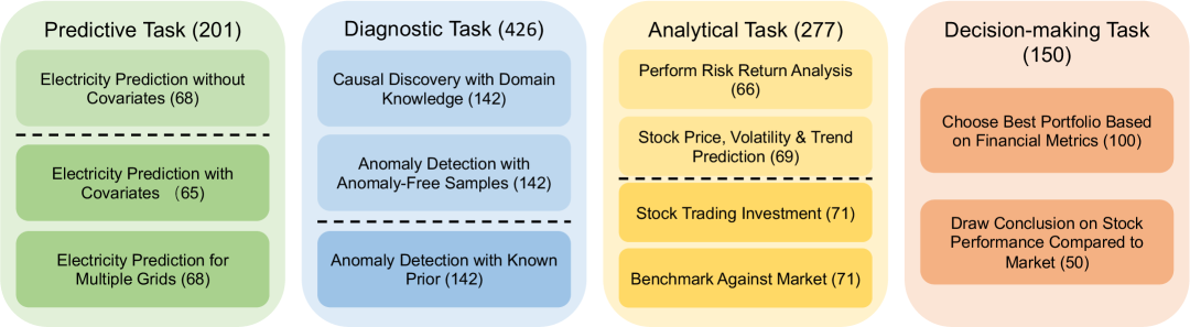
To evaluate time series AI assistants effectively, we focus on tasks grounded in real-world use cases that data analyst in different time series application domains may face. We aim for the tasks to assess an assistant’s ability to handle practical scenarios involving time series data, ensuring their utility in everyday analytical workflows. We start by forming a group of three graduate students with backgrounds in machine learning and applied time series analysis to collect real world applications of time series analysis that exhibit multi-step complexity and requires reasoning. We reviewed over 20 research publications addressing time series analysis challenges, extracting and converting core problems into benchmark tasks. The collected tasks can be categorized into four broad groups based on the nature of the underlying problem as shown in figure 1: (1) Predictive Tasks involve forecasting with or without covariates, with constraint-aware prediction that must comply with real-world operational requirements such as maximum/minimum load limits wang220kv ; greif1999short , ramp rate constraints schaible2024application ; gkavanoudis2023provision , and variability thresholds han2021real . (2) Diagnostic Tasks focus on identifying abnormal patterns or latent structures within the data. This includes anomaly detection tasks, which may leverage reference samples or known anomaly frequencies yan2021learning ; song2024unsupervised ; niu2020lstm ; verma2023deep ; and causal discovery tasks, where models infer binary causal graphs from observational time series with domain-specific priors such as partial causal ratios or qualitative relationships aoki2020parkca . (3) Analytical Tasks target analytics based on time series trends, particularly within financial domains. These tasks may require performing risk-return analysis riley2022maximum ; miglietti2020bitcoin or generating trading strategies using historical asset prices shalini2019picking ; pramudya2020technical . (4) Decision-Making Tasks are framed as multiple-choice questions, primarily in the financial domain. These require models to analyze structured summaries such as portfolio performance under different metrics steinki2015common or compare a stock’s performance to a market index gupta1999information . The correct answer involves selecting the option that best aligns with the target financial principle, testing both computation and reasoning legrenzi1993focussing .
For each task, we manually craft task templates based on extracted problem formulations, collect and preprocess the relevant datasets, and, where appropriate, appended domain-specific metadata. Time series datasets in TSAIA are collected from publicly available repositories spanning domains including energy management, climate science, finance, and healthcare. Specifically, it incorporates electricity grid load data, solar and wind power measurements with corresponding weather covariates zheng2021psml 111CC BY 4.0 licence;
† Open Data Commons Attribution 1.0 licence.
‡ Yahoo Finance Terms of Service: personal, non-commercial use only., building energy usage patterns LEAD2022 111CC BY 4.0 licence;
† Open Data Commons Attribution 1.0 licence.
‡ Yahoo Finance Terms of Service: personal, non-commercial use only., ERA5 climate variables hersbach2020era5 111CC BY 4.0 licence;
† Open Data Commons Attribution 1.0 licence.
‡ Yahoo Finance Terms of Service: personal, non-commercial use only., MIT-BIH ECG signals goldberger2000physiobank †, and economic indicators such as stock indices and individual stock prices yahoo_finance ‡.
2.2 Question Generator: How to generate specific task instances?
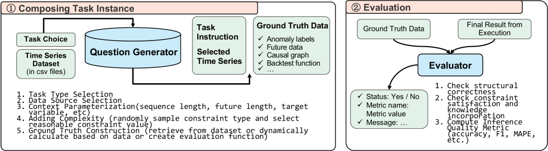
We design a modular and programmatic pipeline (illustrated in figure 2) to generate diverse task instances for evaluating time series inference tasks. The generation process proceeds in five steps: (1) Task Type Selection: The generation process begins by selecting a task type from a predefined library. (2) Data Source Selection: A time series dataset is sampled from a repository of CSV datasets. (3) Context Parameterization: Once a dataset is selected, the generator randomly configures instance-specific parameters such as input sequence length, forecasting horizon (if applicable), target variable, covariate inclusion. These contextual parameters are crucial for defining the scope of the task instance. The natural language template corresponding to the selected task type is dynamically populated with the sampled parameters and contextual information. (4) Adding Complexity: To reflect real-world conditions, the generator samples domain-specific constraints or auxiliary knowledge defined by the task template and adds to the task instruction. (5) Ground Truth Construction: Finally, ground truth solutions are either directly retrieved from the dataset, dynamically computed based on the task parameters, or delegated to domain-specific evaluation functions. This step ensures that each instance is paired with an executable reference output, enabling robust automatic evaluation.
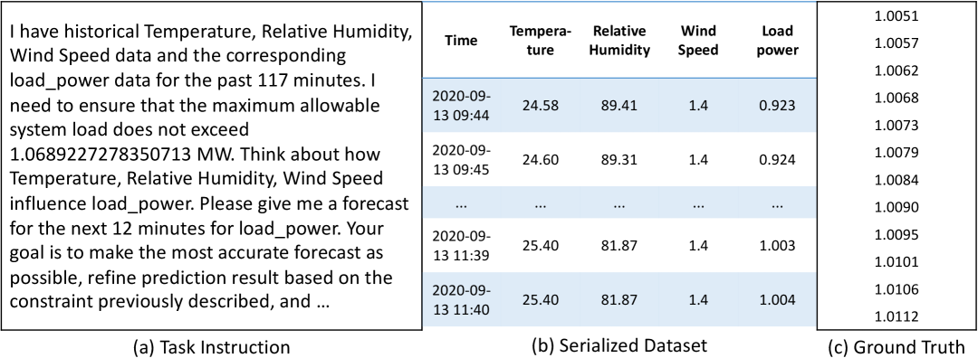
As shown in figure 3, each task instance contains a natural language instruction paired with structured time series inputs and corresponding ground truth data. By design, the benchmark framework is extensible and dynamic. New task instances can be generated automatically by applying the same pipeline to additional time series data sources when accompanied by its designated task template, supporting ongoing evaluation and adaptation to new domains. This supports long-term benchmarking efforts and enables ongoing expansion across domains.
2.3 Evaluation: How to perform evaluation on heterogeneous task instances?
| Task Type | Success Criterion | Metrics |
|---|---|---|
| Constrained Forecasting | Prediction is of correct shape and satisfies the specified operational constraint and the prediction is non-trivial (MAPE<1) | MAPE |
| Anomaly Detection w/ reference samples | A binary sequence with correct length is obtained and the prediction is non-trivial (F1-score>0) | F1-score |
| Causal Inference w/ domain knowledge | A binary causal matrix with correct shape is returned. The provided domain knowledge is incorporated | Accuracy |
| Financial Analytics | A scalar value is returned and the prediction is non-trivial (absolute error<0.05) | Absolute Error |
| Financial Trading | An investment signal of correct length is returned and there is no loss in investment | CR, AR, MDD |
Ground Truth Data
Ground truth labels are defined based on the task type and the nature of the expected output. For questions demanding numerical outputs, the ground truth is obtained through one of three mechanisms. (1) Retrieved from dataset: For predictive tasks, the ground truth corresponds to the future values of the target variable over the specified forecasting horizon. In diagnostic tasks such as anomaly detection, binary anomaly labels serve as ground truth for the given time window. (2) Dynamically computed based on data: In risk & return analysis, ground truth values are derived based on predefined formulas for key performance metrics and are dynamically computed based on data. (3) Defined by an evaluation function: In contrast, trading tasks do not have a unique ground truth strategy, as multiple plausible investment approaches may yield positive returns. Instead of comparing predicted strategies to a reference solution, we evaluate the generated investment signals through backtesting on held-out stock price data over the hypothetical investment period. Performance is assessed using financial metrics such as cumulative return clarke2011minimum , annualized return booth1992diversification , and maximum drawdown magdon2004maximum .
For multiple-choice questions, the answer is determined through quantitative evaluation. In portfolio-based questions, each option corresponds to a distinct portfolio constructed from sampled stocks and associated holding ratios, and the correct answer is the portfolio that optimizes the target metric such as Sharpe ratio sharpe1994sharpe , Value at Risk duffie1997overview based on selected data. In stock-versus-market comparisons, ground truth relationship between the stock and market is derived from computed indicators Jensen’s alpha and beta fisher2018risk . To avoid positional bias, correct answers are randomly assigned to lettered choices, ensuring a uniform distribution across answer positions throughout the dataset.
| Benchmark | Dynamic | TS involved | Reasoning | #Tasks | Task Type |
| Test of Time fatemi2024test | ✗ | ✗ | ✓ | 1 | QA |
| TRAM wang2024tram | ✗ | ✗ | ✓ | 1 | QA |
| TSI-Bench du2024tsi | ✗ | ✓ | ✗ | 1 | TS Analysis |
| TSB-AD liu2024the | ✗ | ✓ | ✗ | 1 | TS Analysis |
| GIFT-Eval aksugift | ✗ | ✓ | ✗ | 1 | TS Analysis |
| TFB qiu2024tfb | ✗ | ✓ | ✗ | 1 | TS Analysis |
| Time-MMD liu2024timemmd | ✗ | ✓ | ✗ | 1 | TS Analysis |
| CiK williams2024context | ✗ | ✓ | ✗ | 1 | TS Analysis |
| TGTSF xu2024beyond | ✗ | ✓ | ✗ | 1 | TS Analysis |
| LLM TS Struggle merrill2024language | ✗ | ✓ | ✓ | 2 | QA, TS Analysis |
| MTBench chen2025mtbench | ✗ | ✓ | ✓ | 3 | QA, TS Analysis |
| ChatTime chatime | ✗ | ✓ | ✓ | 3 | QA, TS Analysis |
| TSAIA(Ours) | ✓ | ✓ | ✓ | 4 | QA, TS Analysis |
Evaluation Criteria
Given the diverse nature of the tasks—ranging from numerical forecasting to causal inference and constraint satisfaction—it is neither appropriate nor effective to rely on a single evaluation metric. Instead, evaluation must be tailored to each task to ensure a meaningful assessment of model performance. Across all tasks, outputs must conform to expected formats, satisfy any injected constraints, and appropriately incorporate provided domain knowledge. Trivial or degenerate outputs such as poor quality predictions or all-zero anomaly labels are flagged as failures, even if their format is technically correct. Each task type is governed by well-defined success criteria and inference quality metrics, designed to reflect practical expectations of correctness and utility. Table 1 summarizes the criteria used for each task.
The evaluation process follows a three-stage protocol. In the first stage, outputs are validated for structural correctness, shape conformity. The second stage checks against specified constraint and domain knowledge incorporation. Lastly, the inference quality metric is computed relative to ground truth data. Results are returned in a structured format, including the success status, diagnostic messages, and detailed metric scores. Failures are categorized into execution errors (model output fails to run or parse), constraint violations (outputs violate injected domain-specific rules), and low quality outputs (predictions meet format expectations but fall short on metric thresholds). Multiple choice questions have a simple evaluation procedure of checking against ground truth letter option.
2.4 Comparison with Existing Benchmarks
As shown in table 2, existing time-series benchmarks fall into three main groups, each lacking one or more component for evaluating time series AI assistant: First, datasets such as Test of Time fatemi2024test and TRAM wang2024tram present pure QA tasks (ordering, duration, arithmetic) with no time-series included (TS involved:✗). While they evaluate logical reasoning, they cannot test how models process numerical signals. Secondly, benchmarks like TSI-Bench du2024tsi , TSB-AD liu2024the , GIFT-Eval aksugift , TFB qiu2024tfb , Time-MMD liu2024timemmd , CiK williams2024context , and TGTSF xu2024beyond focus on a single static time‐series analysis including imputation, anomaly detection, and forecasting over fixed datasets with pre-defined sliding window size for evaluation (Dynamic:✗, Reasoning:✗, Tasks=1). Lastly, recent efforts on hybrid QA and analysis such as MTBench chen2025mtbench , ChatTime chatime combine time-series and text inputs (TS involved:✓) and include reasoning components (Reasoning:✓), yet remain fixed setting (Dynamic:✗) and only covers context-aided forecasting in time series analysis component part. TSAIA arises as first of its kind time series inference benchmark with practical relevance, task diversity, and supports continuous expansion.
3 Experiments
| Metric | GPT-4o | Qwen-Max | Llama3.1 | Claude-3.5 | DeepSeek | Gemini-2.0 | Codestral | DeepSeek-R | |
|---|---|---|---|---|---|---|---|---|---|
| Electricity Prediction with Covariates | |||||||||
| Max Load | Success Rate | 0.50 | 0.75 | 0.56 | 0.88 | 1.00 | 0.19 | 0.31 | 0.94 |
| MAPE (std) | 0.09 (0.12) | 0.07 (0.06) | 0.10 (0.11) | 0.11 (0.12) | 0.10 (0.12) | 0.52 (0.41) | 0.03 (0.03) | 0.10 (0.11) | |
| Min Load | Success Rate | 0.76 | 0.82 | 0.65 | 0.82 | 0.88 | 0.18 | 0.59 | 1.00 |
| MAPE (std) | 0.11 (0.11) | 0.09 (0.11) | 0.10 (0.11) | 0.09 (0.11) | 0.12 (0.18) | 0.09 (0.04) | 0.09 (0.10) | 0.09 (0.11) | |
| Load Ramp Rate | Success Rate | 0.46 | 0.80 | 0.53 | 0.93 | 0.80 | 0.13 | 0.47 | 0.93 |
| MAPE (std) | 0.18 (0.14) | 0.14 (0.12) | 0.15 (0.07) | 0.19 (0.19) | 0.11 (0.08) | 0.04 (0.01) | 0.12 (0.08) | 0.11 (0.07) | |
| Load Variability | Success Rate | 0.47 | 0.76 | 0.29 | 0.29 | 0.76 | 0.06 | 0.35 | 0.94 |
| MAPE (std) | 0.20 (0.31) | 0.13 (0.16) | 0.09 (0.12) | 0.09 (0.12) | 0.19 (0.27) | 0.05 (0.00) | 0.04 (0.03) | 0.11 (0.14) | |
| Electricity Prediction without Covariates | |||||||||
| Max Load | Success Rate | 1.00 | 0.94 | 0.94 | 1.00 | 0.94 | 0.41 | 1.00 | 0.71 |
| MAPE (std) | 0.18 (0.16) | 0.10 (0.07) | 0.16 (0.10) | 0.15 (0.13) | 0.15 (0.12) | 0.10 (0.02) | 0.12 (0.07) | 0.23 (0.26) | |
| Min Load | Success Rate | 0.94 | 0.94 | 0.94 | 0.94 | 0.88 | 0.29 | 0.71 | 0.88 |
| MAPE (std) | 0.14 (0.08) | 0.14 (0.08) | 0.17 (0.08) | 0.17 (0.09) | 0.13 (0.09) | 0.12 (0.03) | 0.14 (0.05) | 0.17 (0.16) | |
| Load Ramp Rate | Success Rate | 0.76 | 1.00 | 0.71 | 0.76 | 0.82 | 0.24 | 0.88 | 0.76 |
| MAPE (std) | 0.24 (0.19) | 0.23 (0.22) | 0.21 (0.11) | 0.28 (0.16) | 0.19 (0.20) | 0.42 (0.28) | 0.29 (0.30) | 0.22 (0.13) | |
| Load Variability | Success Rate | 0.82 | 0.88 | 0.82 | 0.65 | 0.76 | 0.41 | 0.71 | 0.65 |
| MAPE (std) | 0.17 (0.12) | 0.13 (0.09) | 0.15 (0.09) | 0.16 (0.12) | 0.19 (0.17) | 0.39 (0.39) | 0.13 (0.07) | 0.24 (0.24) | |
| Electricity Prediction for Multiple Grids | |||||||||
| Max Load | Success Rate | 0.76 | 0.88 | 0.47 | 0.88 | 0.94 | 0.47 | 0.12 | 0.88 |
| MAPE (std) | 0.21 (0.27) | 0.21 (0.24) | 0.64 (0.31) | 0.18 (0.20) | 0.16 (0.21) | 0.34 (0.39) | 0.10 (0.03) | 0.23 (0.27) | |
| Min Load | Success Rate | 0.76 | 0.88 | 0.24 | 0.94 | 0.94 | 0.18 | 0.29 | 0.94 |
| MAPE (std) | 0.10 (0.12) | 0.18 (0.29) | 0.46 (0.37) | 0.13 (0.20) | 0.08 (0.11) | 0.01 (0.01) | 0.23 (0.37) | 0.16 (0.23) | |
| Load Ramp Rate | Success Rate | 0.65 | 0.65 | 0.88 | 0.88 | 0.94 | 0.29 | 0.29 | 1.00 |
| MAPE (std) | 0.19 (0.24) | 0.18 (0.18) | 0.73 (0.33) | 0.27 (0.21) | 0.21 (0.21) | 1.00 (0.00) | 0.10 (0.05) | 0.19 (0.19) | |
| Load Variability | Success Rate | 0.41 | 0.59 | 0.53 | 0.41 | 0.59 | 0.35 | 0.29 | 0.53 |
| MAPE (std) | 0.15 (0.13) | 0.18 (0.23) | 0.61 (0.36) | 0.11 (0.13) | 0.18 (0.14) | 0.90 (0.23) | 0.19 (0.13) | 0.24 (0.25) | |
| Benchmark | GPT-4o | Qwen-Max | Llama3.1 | Claude-3.5 | DeepSeek | Gemini-2.0 | Codestral | DeepSeek-R | |
|---|---|---|---|---|---|---|---|---|---|
| Diagnostic Task w/ Reference Samples | |||||||||
| Extreme Weather Detection | Success Rate | 0.24 | 0.23 | 0.23 | 0.62 | 0.23 | 0.14 | 0.23 | 0.34 |
| w/ Reference Samples | F1 (std) | 0.91 (0.23) | 0.90 (0.24) | 0.90 (0.24) | 0.90 (0.18) | 0.90 (0.24) | 0.96 (0.06) | 0.91 (0.23) | 0.91 (0.20) |
| ECG Signal Anomaly | Success Rate | 0.51 | 0.17 | 0.55 | 0.68 | 0.54 | 0.10 | 0.59 | 0.63 |
| w/ Reference Samples | F1 (std) | 0.55 (0.35) | 0.70 (0.29) | 0.43 (0.36) | 0.65 (0.32) | 0.54 (0.34) | 0.01 (0.00) | 0.58 (0.34) | 0.61 (0.32) |
| Causal Discovery w/ Domain Knowledge | |||||||||
| Causal Discovery w/ | Success Rate | 0.94 | 0.92 | 0.99 | 1.00 | 0.97 | 0.39 | 0.94 | 0.96 |
| Quantitative Knowledge | Accuracy (std) | 0.69 (0.09) | 0.77 (0.11) | 0.78 (0.12) | 0.77 (0.09) | 0.71 (0.11) | 0.42 (0.18) | 0.72 (0.11) | 0.77 (0.10) |
| Causal Discovery w/ | Success Rate | 0.85 | 0.70 | 0.83 | 0.97 | 0.96 | 0.45 | 0.93 | 0.99 |
| Qualitative Knowledge | Accuracy (std) | 0.87 (0.17) | 0.79 (0.17) | 0.77 (0.18) | 0.89 (0.16) | 0.89 (0.14) | 0.72 (0.20) | 0.88 (0.15) | 0.90 (0.12) |
| Anomaly Detection across Multiple Sequences | |||||||||
| Extreme Weather Detection | Success Rate | 0.87 | 0.31 | 0.03 | 0.97 | 0.97 | 0.37 | 0.23 | 1.00 |
| w/ Known Anomaly Rate | F1 (std) | 0.53 (0.25) | 0.62 (0.19) | 0.68 (0.05) | 0.73 (0.12) | 0.72 (0.11) | 0.65 (0.18) | 0.42 (0.31) | 0.72 (0.10) |
| Energy Usage Anomaly | Success Rate | 0.87 | 0.52 | 0.77 | 1.00 | 1.00 | 0.23 | 0.58 | 0.96 |
| w/ Known Anomaly Rate | F1 (std) | 0.08 (0.09) | 0.14 (0.20) | 0.15 (0.11) | 0.48 (0.18) | 0.50 (0.19) | 0.19 (0.21) | 0.06 (0.06) | 0.40 (0.23) |
| Benchmark | GPT-4o | Qwen-Max | Llama3.1 | Claude-3.5 | DeepSeek | Gemini-2.0 | Codestral | DeepSeek-R | |
|---|---|---|---|---|---|---|---|---|---|
| Stock Prediction | |||||||||
| Future Price | Success Rate | 0.96 | 1.00 | 0.70 | 0.74 | 0.87 | 0.17 | 0.39 | 1.00 |
| MAPE (std) | 0.06 (0.08) | 0.05 (0.07) | 0.06 (0.08) | 0.12 (0.16) | 0.05 (0.07) | 0.28 (0.42) | 0.05 (0.05) | 0.05 (0.07) | |
| Future Volatility | Success Rate | 0.83 | 0.43 | 0.39 | 0.74 | 0.57 | 0.17 | 0.57 | 0.61 |
| MAPE (std) | 0.70 (0.28) | 0.83 (0.26) | 0.64 (0.29) | 0.75 (0.31) | 0.90 (0.13) | 0.84 (0.24) | 0.61 (0.32) | 0.77 (0.24) | |
| Future Trend | Success Rate | 0.43 | 0.30 | 0.57 | 0.26 | 0.43 | 0.04 | 0.52 | 0.35 |
| Accuracy (std) | 0.90 (0.20) | 0.86 (0.23) | 0.88 (0.21) | 1.00 (0.00) | 0.85 (0.23) | 1.00 (0.00) | 0.96 (0.14) | 0.81 (0.24) | |
| Risk/Return Estimation | |||||||||
| Annualized Return | Success Rate | 0.45 | – | 0.09 | 0.27 | 0.36 | – | 0.18 | 0.55 |
| Abs Error (std) | 0.02 (0.02) | – | 0.01 (0.00) | 0.01 (0.01) | 0.02 (0.01) | – | 0.03 (0.02) | 0.02 (0.02) | |
| Annualized Volatility | Success Rate | 0.91 | 0.82 | 1.00 | 1.00 | 1.00 | 0.09 | 1.00 | 0.91 |
| Abs Error (std) | 0.00 (0.00) | 0.00 (0.00) | 0.00 (0.00) | 0.00 (0.00) | 0.00 (0.00) | 0.02 (0.00) | 0.00 (0.00) | 0.00 (0.00) | |
| Maximum Drawdown | Success Rate | 0.18 | 0.09 | 0.27 | 0.18 | 0.27 | 0.09 | – | 0.45 |
| Abs Error (std) | 0.00 (0.00) | 0.00 (0.00) | 0.00 (0.00) | 0.00 (0.00) | 0.00 (0.00) | 0.00 (0.00) | – | 0.01 (0.01) | |
| Calmar Ratio | Success Rate | 0.18 | 0.18 | – | 0.27 | 0.27 | – | 0.82 | 0.18 |
| Abs Error (std) | 0.01 (0.01) | 0.01 (0.01) | – | 0.02 (0.01) | 0.02 (0.01) | – | 0.01(0.01) | 0.01 (0.01) | |
| Sortino Ratio | Success Rate | 0.09 | 0.09 | – | – | 0.18 | – | 0.09 | – |
| Abs Error (std) | 0.01 (0.00) | 0.01 (0.00) | – | – | 0.00 (0.00) | – | 0.00 (0.00) | – | |
| Sharpe Ratio | Success Rate | 0.73 | 0.18 | 0.27 | 0.36 | 0.18 | 0.18 | 0.73 | 0.18 |
| Abs Error (std) | 0.00 (0.00) | 0.00 (0.00) | 0.00 (0.00) | 0.01 (0.01) | 0.02 (0.02) | 0.02 (0.02) | 0.00 (0.00) | 0.02 (0.01) | |
| Benchmark Against Market Analysis | |||||||||
| Information Ratio | Success Rate | 0.44 | 0.20 | 0.06 | 0.51 | 0.73 | 0.18 | 0.01 | 0.77 |
| Abs Error (std) | 0.00 (0.00) | 0.01 (0.01) | 0.03 (0.01) | 0.00 (0.01) | 0.00 (0.00) | 0.00 (0.01) | 0.00 (0.00) | 0.00 (0.00) | |
| Stock Trading Strategy | |||||||||
| Trading Strategy | Success Rate | 0.44 | 0.59 | 0.96 | 0.62 | 0.61 | 0.18 | 0.63 | 0.52 |
| Cumulative Return | 0.13 | 0.10 | 0.00 | 0.09 | 0.09 | 0.05 | 0.06 | 0.07 | |
| Annualized Return | 2.43 | 4.56 | 0.05 | 4.58 | 1.69 | 0.36 | 3.87 | 1.41 | |
| Maximum Drawdown | 0.05 | 0.05 | 0.00 | 0.04 | 0.05 | 0.02 | 0.02 | 0.04 | |
3.1 Experimental Setup
We evaluate the performance of eight large language models (LLMs) on the full suite of benchmark tasks, covering both open-source and proprietary systems: GPT-4o hurst2024gpt , Qwen2.5-Max qwen2025max , Llama-3.1 Instruct 70b grattafiori2024llama , Claude-3.5 Sonnet anthropic2024claude35sonnet , DeepSeek liu2024deepseek , Gemini-2.0 google2024gemini2 , Codestral mistral2024codestral , and DeepSeek-R guo2025deepseek . Among them, Llama3.1 Instruct 70B serves as a representative open-weight model, Codestral is a code-specialized model built upon Mistral mistral2024homepage , and DeepSeek-Reasoner is a novel model designed explicitly for complex reasoning tasks. To address LLMs’ limitations in processing structured numerical inputs and producing high-precision, correctly shaped numerical outputs, we adopt the CodeAct wang2024executable agent framework for all models. Agentscope CodeAct agent agentscope enables code-based interaction by allowing LLMs to generate executable Python code, receive execution feedback, and revise outputs accordingly. All models are accessed via their official APIs and ran on a single NVIDIA A40 GPU with 48G memory. For all experiments, we use the same hyperparameters, temperature=0.0 for the most deterministic output and top_p=1.0.
For each benchmark task, models are provided with the same input data, including a task instruction and a serialized time series dataset in .pkl format. Responses are executed within a controlled jupyter notebook python interpreter provided by CodeAct agent setup. The final outputs are passed to task-specific evaluators, which extract predictions and compute metrics based on ground truth labels or evaluation programs. Each model’s performance is assessed using two main criteria: The primary metric is Success Rate which is defined as the proportion of task instances for which the model output satisfies the predefined success criteria (see Table 1). For outputs deemed successful, we further evaluate quality using task-specific metrics (e.g., MAPE for forecasting, F1-score for anomaly detection), providing a more fine-grained comparison of inference quality.
3.2 Result
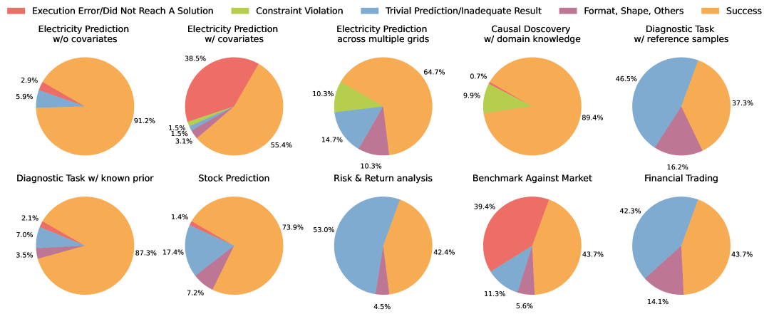
We report model performance across four primary task categories: predictive, diagnostic, analytical. and decision-making tasks. Predictive tasks involve forecasting under real-world operational constraints. As shown in table 3, models generally perform well on simpler constraints (maximum or minimum load) but struggle with tasks requiring temporal smoothness (ramp rate or variability control). Forecasting tasks on multiple grids introduce greater complexity due to increased data volume and dimensionality. This is reflected in lower success rates and higher MAPE values across all models. For diagnostic tasks, models show moderate success on anomaly detection with known priors. When anomaly-free reference samples are available (e.g., in extreme weather or ECG tasks), models must learn how to calibrate thresholds before detecting deviations. However, results in Table 4 reveal that models struggle to meaningfully use reference samples, often returning trivial predictions evidenced by the case study in figure 7. This reflects a broader limitation: current LLMs have difficulty autonomously assembling complex workflows such as leveraging reference sequences to calibrate thresholds. These findings are consistent with prior research indicating that transformer-based LLMs often lack systematic compositional reasoning capabilities, instead relying on pattern matching, which hampers their performance in tasks requiring multi-step reasoning dziri2023faith .
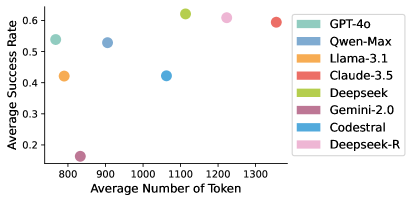
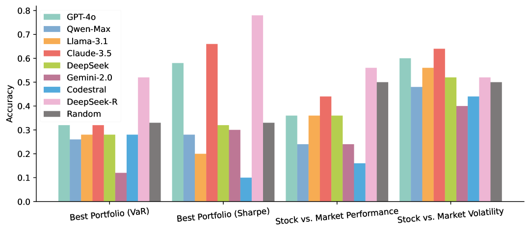
In financial forecasting, models show moderate-to-strong performance on price and volatility prediction. However, trend prediction remains a challenge across all models, with lower success rate and accuracy shown in table 5. In performing risk and return analysis, success rates vary widely, and models appear biased toward metrics with simpler formulas (e.g., annualized volatility) or greater familiarity (e.g., Sharpe ratio).This suggests that financial metric familiarity and formula simplicity also affects model behavior. In multiple-choice question formats testing financial reasoning, most models fail to exceed chance-level accuracy as shown in figure 5. DeepSeek-R stands out as the only model demonstrating consistent, above-random performance across portfolio and stock market comparison tasks. However, it’s important to note that DeepSeek-R also consistently uses more tokens in solving a single question shown in figure 4. Overall, our results underscore the importance of domain specialization ling2023domain in LLMs, as general-purpose models often struggle with the unique challenges presented by specialized data domains and application fields.
Analysis
We analyze agent behavior across difficulty levels by measuring the average number of interaction turns each model uses to solve a task (Figure 6). The maximum number of turns is capped at 6 under the CodeAct agent framework. Across all task categories, harder tasks generally require more interaction turns, confirming the importance of model–execution feedback loops for solution refinement. Notably, DeepSeek-R consistently takes more turns compared to other models—indicating a more persistent, exploratory problem-solving strategy. This behavior correlates with higher token usage, as shown in Figure 4. When accounting for cost efficiency (also illustrated in Figure 4), GPT-4o and DeepSeek-Chat emerge as the most token-efficient models.
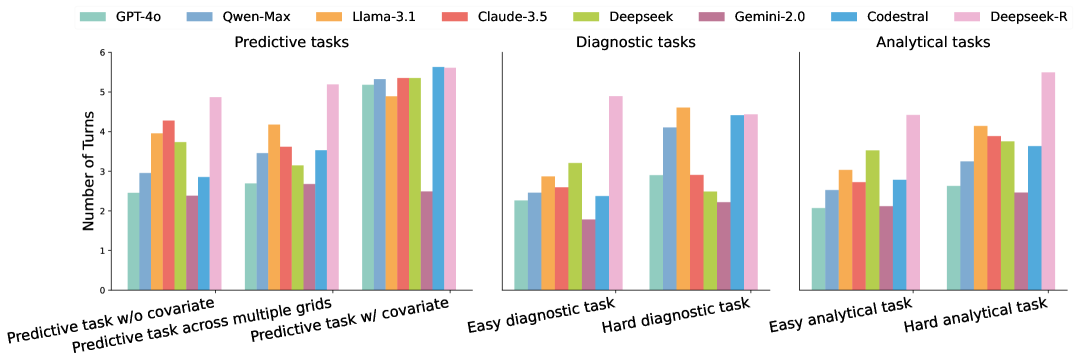
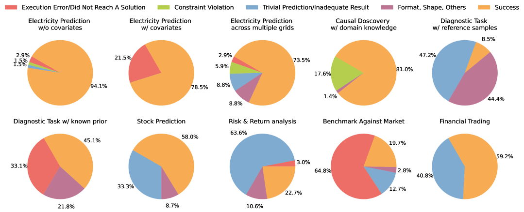
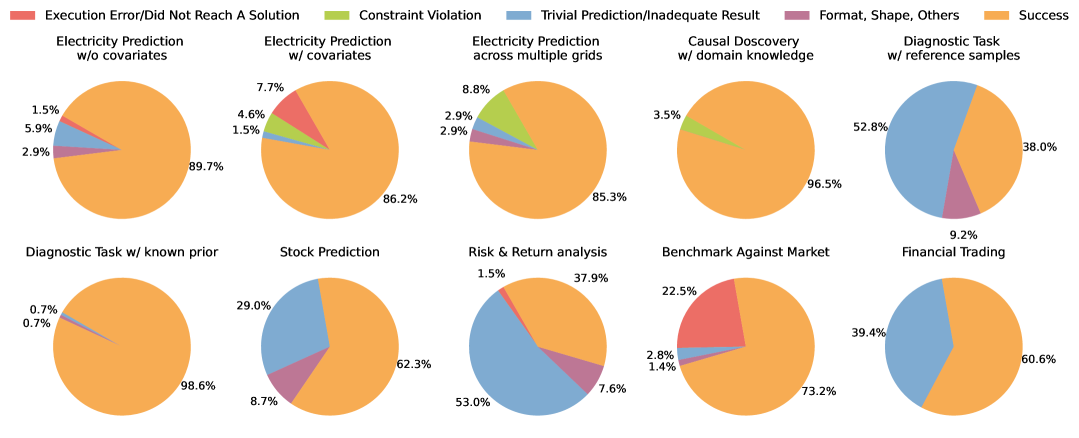
Figure 7 presents a detailed breakdown of GPT-4o’s error distribution across various task types. Within predictive tasks, incorporating covariates introduces additional complexity and results in a higher incidence of execution errors. Further, when the forecasting task spans multiple time series, maintaining operational constraints such as ramp rates and load bounds becomes substantially more difficult, leading to a greater frequency of constraint violation errors compared to the simpler single-series settings.
In diagnostic tasks, the use of reference samples introduces a form of contextual reasoning: the model is expected to use anomaly-free samples to calibrate thresholds for anomaly detection. GPT-4o struggles with this setup, and trivial predictions such as all-zero anomaly label emerge as the dominant failure mode. This suggests an inability to orchestrate the multi-step workflow needed for threshold calibration, which involves abstract reasoning over auxiliary context. In contrast, tasks where domain knowledge is explicitly provided such as causal discovery with known graph structure or diagnostic tasks with priors exhibit relatively high success rates. The structured nature of this prior knowledge makes it easier for the model to align its output accordingly.
Among analytical tasks, benchmarking against the market poses the greatest challenge, marked by a high proportion of execution errors. This can be attributed to the model’s need to simultaneously process both stock-specific and market-wide indicators. For risk and return analysis, the most common failure type is inadequate results, stemming from the model’s limited familiarity with less conventional financial metrics. A similar pattern is observed in financial trading where the generated investment strategy is often suboptimal, resulting in poor returns during backtesting. This outcome highlights the inherent difficulty of trading tasks, which require both strategic reasoning and financial acumen. Overall, the distribution of errors reveals a clear trend: as tasks demand more structured multi-step reasoning, integration of external context, or nuanced financial understanding, GPT-4o’s reliability decreases and its failure modes become more diverse.
4 Conclusion
This paper introduces TSAIA, a first attempt for evaluating LLMs as time series AI assistants. Spanning predictive, diagnostic, analytical, and financial decision-making categories, the benchmark emphasizes compositional reasoning, adherence to domain-specific constraints, and the integration of contextual knowledge. While the current scale of TSAIA is limited, we prioritize task quality, diversity, and alignment with real-world analytical workflows over quantity. Future extensions will broaden domain coverage and increase task instance variety to further challenge LLMs to perform complex multi-step time series analysis tasks. Our extensive evaluation of eight LLM agents reveals limitations in their performance when complex domain constraints or multi-step workflows are involved. Results highlight the need for hybrid approaches that tightly integrate symbolic reasoning, execution feedback, and domain alignment. TSAIA provides a foundation for such progress, enabling systematic assessment and facilitating the development of next-generation time series inference agents, with potential applications across critical sectors such as energy, finance, and healthcare.
References
- [1] Li Dong, Nan Yang, Wenhui Wang, Furu Wei, Xiaodong Liu, Yu Wang, Jianfeng Gao, Ming Zhou, and Hsiao-Wuen Hon. Unified language model pre-training for natural language understanding and generation. Advances in neural information processing systems, 32, 2019.
- [2] Juyong Jiang, Fan Wang, Jiasi Shen, Sungju Kim, and Sunghun Kim. A survey on large language models for code generation. arXiv preprint arXiv:2406.00515, 2024.
- [3] Ross Taylor, Marcin Kardas, Guillem Cucurull, Thomas Scialom, Anthony Hartshorn, Elvis Saravia, Andrew Poulton, Viktor Kerkez, and Robert Stojnic. Galactica: A large language model for science. arXiv preprint arXiv:2211.09085, 2022.
- [4] Francisco Martinez Alvarez, Alicia Troncoso, Jose C Riquelme, and Jesus S Aguilar Ruiz. Energy time series forecasting based on pattern sequence similarity. IEEE Transactions on Knowledge and Data Engineering, 23(8):1230–1243, 2010.
- [5] Omer Berat Sezer, Mehmet Ugur Gudelek, and Ahmet Murat Ozbayoglu. Financial time series forecasting with deep learning: A systematic literature review: 2005–2019. Applied soft computing, 90:106181, 2020.
- [6] Manfred Mudelsee. Trend analysis of climate time series: A review of methods. Earth-science reviews, 190:310–322, 2019.
- [7] Niels K Rathlev, John Chessare, Jonathan Olshaker, Dan Obendorfer, Supriya D Mehta, Todd Rothenhaus, Steven Crespo, Brendan Magauran, Kathy Davidson, Richard Shemin, et al. Time series analysis of variables associated with daily mean emergency department length of stay. Annals of emergency medicine, 49(3):265–271, 2007.
- [8] Xudong Yan, Huaidong Zhang, Xuemiao Xu, Xiaowei Hu, and Pheng-Ann Heng. Learning semantic context from normal samples for unsupervised anomaly detection. In Proceedings of the AAAI conference on artificial intelligence, volume 35, pages 3110–3118, 2021.
- [9] Kyo Beom Han, Jaesung Jung, and Byung O Kang. Real-time load variability control using energy storage system for demand-side management in south korea. Energies, 14(19):6292, 2021.
- [10] Yao Fu, Hao Peng, Ashish Sabharwal, Peter Clark, and Tushar Khot. Complexity-based prompting for multi-step reasoning. arXiv preprint arXiv:2210.00720, 2022.
- [11] Kostadin Cvejoski, Ramsés J Sánchez, and César Ojeda. The future is different: Large pre-trained language models fail in prediction tasks. arXiv preprint arXiv:2211.00384, 2022.
- [12] Zhiyi Xue, Liangguo Li, Senyue Tian, Xiaohong Chen, Pingping Li, Liangyu Chen, Tingting Jiang, and Min Zhang. Domain knowledge is all you need: A field deployment of llm-powered test case generation in fintech domain. In Proceedings of the 2024 IEEE/ACM 46th International Conference on Software Engineering: Companion Proceedings, pages 314–315, 2024.
- [13] Ke-qiu WANG, Si-guang SUN, Hong-yi WANG, Chang-xu JIANG, and Zhao-xia JING. 220kv city power grid maximum loadability determination with static security-constraints. Power, Energy Engineering and Management (PEEM2016), page 1, 2016.
- [14] Mike A Merrill, Mingtian Tan, Vinayak Gupta, Thomas Hartvigsen, and Tim Althoff. Language models still struggle to zero-shot reason about time series. In EMNLP (Findings), 2024.
- [15] Wenjie Du, Jun Wang, Linglong Qian, Yiyuan Yang, Zina Ibrahim, Fanxing Liu, Zepu Wang, Haoxin Liu, Zhiyuan Zhao, Yingjie Zhou, et al. Tsi-bench: Benchmarking time series imputation. arXiv preprint arXiv:2406.12747, 2024.
- [16] Haoyi Zhou, Shanghang Zhang, Jieqi Peng, Shuai Zhang, Jianxin Li, Hui Xiong, and Wancai Zhang. Informer: Beyond efficient transformer for long sequence time-series forecasting. In Proceedings of the AAAI conference on artificial intelligence, volume 35, pages 11106–11115, 2021.
- [17] Yuqing Wang and Yun Zhao. Tram: Benchmarking temporal reasoning for large language models. In Findings of the Association for Computational Linguistics ACL 2024, pages 6389–6415, 2024.
- [18] Zhaoyi Li, Gangwei Jiang, Hong Xie, Linqi Song, Defu Lian, and Ying Wei. Understanding and patching compositional reasoning in llms. arXiv preprint arXiv:2402.14328, 2024.
- [19] Ernest Davis and Gary Marcus. Commonsense reasoning and commonsense knowledge in artificial intelligence. Communications of the ACM, 58(9):92–103, 2015.
- [20] Aaron Hurst, Adam Lerer, Adam P Goucher, Adam Perelman, Aditya Ramesh, Aidan Clark, AJ Ostrow, Akila Welihinda, Alan Hayes, Alec Radford, et al. Gpt-4o system card. arXiv preprint arXiv:2410.21276, 2024.
- [21] Qwen Team. Qwen2.5-max: Exploring the intelligence of large-scale moe model, January 2025. Accessed: 2025-05-14.
- [22] Aaron Grattafiori, Abhimanyu Dubey, Abhinav Jauhri, Abhinav Pandey, Abhishek Kadian, Ahmad Al-Dahle, Aiesha Letman, Akhil Mathur, Alan Schelten, Alex Vaughan, et al. The llama 3 herd of models. arXiv preprint arXiv:2407.21783, 2024.
- [23] Anthropic. Claude 3.5 sonnet, June 2024. Accessed: 2025-05-14.
- [24] Aixin Liu, Bei Feng, Bing Xue, Bingxuan Wang, Bochao Wu, Chengda Lu, Chenggang Zhao, Chengqi Deng, Chenyu Zhang, Chong Ruan, et al. Deepseek-v3 technical report. arXiv preprint arXiv:2412.19437, 2024.
- [25] Google DeepMind. Introducing gemini 2.0: Our new ai model for the agentic era, December 2024. Accessed: 2025-05-14.
- [26] Mistral AI. Codestral, May 2024. Accessed: 2025-05-14.
- [27] Daya Guo, Dejian Yang, Haowei Zhang, Junxiao Song, Ruoyu Zhang, Runxin Xu, Qihao Zhu, Shirong Ma, Peiyi Wang, Xiao Bi, et al. Deepseek-r1: Incentivizing reasoning capability in llms via reinforcement learning. arXiv preprint arXiv:2501.12948, 2025.
- [28] Xingyao Wang, Yangyi Chen, Lifan Yuan, Yizhe Zhang, Yunzhu Li, Hao Peng, and Heng Ji. Executable code actions elicit better llm agents. In Forty-first International Conference on Machine Learning, 2024.
- [29] Dawei Gao, Zitao Li, Xuchen Pan, Weirui Kuang, Zhijian Ma, Bingchen Qian, Fei Wei, Wenhao Zhang, Yuexiang Xie, Daoyuan Chen, Liuyi Yao, Hongyi Peng, Ze Yu Zhang, Lin Zhu, Chen Cheng, Hongzhu Shi, Yaliang Li, Bolin Ding, and Jingren Zhou. Agentscope: A flexible yet robust multi-agent platform. CoRR, abs/2402.14034, 2024.
- [30] Seoha Song, Junhyun Lee, and Hyeonmok Ko. Hansel: Output length controlling framework for large language models. In Proceedings of the AAAI Conference on Artificial Intelligence, volume 39, pages 25146–25154, 2025.
- [31] Dimitris Spathis and Fahim Kawsar. The first step is the hardest: Pitfalls of representing and tokenizing temporal data for large language models. Journal of the American Medical Informatics Association, 31(9):2151–2158, 2024.
- [32] Claudia Greif, Raymond B Johnson, Chao an Li, Alva J Svoboda, and K Andrijeski Uemura. Short-term scheduling of electric power systems under minimum load conditions. IEEE transactions on power systems, 14(1):280–286, 1999.
- [33] Jonas Schaible, Bijan Nouri, Lars Höpken, Tim Kotzab, Matthias Loevenich, Niklas Blum, Annette Hammer, Jonas Stührenberg, Klaus Jäger, Christiane Becker, et al. Application of nowcasting to reduce the impact of irradiance ramps on pv power plants. EPJ Photovoltaics, 15:15, 2024.
- [34] Spyros I Gkavanoudis, Kyriaki-Nefeli D Malamaki, Eleftherios O Kontis, Charis S Demoulias, Aditya Shekhar, Umer Mushtaq, and Sagar Bandi Venu. Provision of ramp-rate limitation as ancillary service from distribution to transmission system: Definitions and methodologies for control and sizing of central battery energy storage system. Journal of Modern Power Systems and Clean Energy, 11(5):1507–1518, 2023.
- [35] Yi Song, Sennan Kuang, Junling Huang, and Da Zhang. Unsupervised anomaly detection of industrial building energy consumption. Energy and Built Environment, 2024.
- [36] Zijian Niu, Ke Yu, and Xiaofei Wu. Lstm-based vae-gan for time-series anomaly detection. Sensors, 20(13):3738, 2020.
- [37] Shikha Verma, Kuldeep Srivastava, Akhilesh Tiwari, and Shekhar Verma. Deep learning techniques in extreme weather events: A review. arXiv preprint arXiv:2308.10995, 2023.
- [38] Raquel Aoki and Martin Ester. Parkca: Causal inference with partially known causes. In BIOCOMPUTING 2021: Proceedings of the Pacific Symposium, pages 196–207. World Scientific, 2020.
- [39] Timothy Riley and Qing Yan. Maximum drawdown as predictor of mutual fund performance and flows. Financial Analysts Journal, 78(4):59–76, 2022.
- [40] Cynthia Miglietti, Zdenka Kubosova, and Nicole Skulanova. Bitcoin, litecoin, and the euro: an annualized volatility analysis. Studies in Economics and Finance, 37(2):229–242, 2020.
- [41] Talwar Shalini, Pranav Shah, and Shah Utkarsh. Picking buy-sell signals: A practitioner’s perspective on key technical indicators for selected indian firms. Studies in Business and Economics, 14(3):205–219, 2019.
- [42] Rommy Pramudya. Technical analysis to determine buying and selling signal in stock trade. International Journal of Finance & Banking Studies (2147-4486), 9(1):58–67, 2020.
- [43] Oliver Steinki and Ziad Mohammad. Common metrics for performance evaluation: Overview of popular performance measurement ratios. Available at SSRN 2662054, 2015.
- [44] Francis Gupta, Robertus Prajogi, and Eric Stubbs. The information ratio and performance. Journal of Portfolio Management, 26(1):33, 1999.
- [45] Paolo Legrenzi, Vittorio Girotto, and Philip N Johnson-Laird. Focussing in reasoning and decision making. Cognition, 49(1-2):37–66, 1993.
- [46] Xiangtian Zheng, Nan Xu, Loc Trinh, Dongqi Wu, Tong Huang, S Sivaranjani, Yan Liu, and Le Xie. Psml: a multi-scale time-series dataset for machine learning in decarbonized energy grids. arXiv preprint arXiv:2110.06324, 2021.
- [47] Large-scale energy anomaly detection (lead). https://www.kaggle.com/competitions/energy-anomaly-detection/data, 2022. Kaggle Competition.
- [48] Hans Hersbach, Bill Bell, Paul Berrisford, Shoji Hirahara, András Horányi, Joaquín Muñoz-Sabater, Julien Nicolas, Carole Peubey, Raluca Radu, Dinand Schepers, et al. The era5 global reanalysis. Quarterly journal of the royal meteorological society, 146(730):1999–2049, 2020.
- [49] Ary L Goldberger, Luis AN Amaral, Leon Glass, Jeffrey M Hausdorff, Plamen Ch Ivanov, Roger G Mark, Joseph E Mietus, George B Moody, Chung-Kang Peng, and H Eugene Stanley. Physiobank, physiotoolkit, and physionet: components of a new research resource for complex physiologic signals. circulation, 101(23):e215–e220, 2000.
- [50] Yahoo Finance. Yahoo Finance, n.d. Accessed: 2025-05-14.
- [51] Roger Clarke, Harindra De Silva, and Steven Thorley. Minimum-variance portfolio composition. Journal of Portfolio Management, 37(2):31, 2011.
- [52] David G Booth and Eugene F Fama. Diversification returns and asset contributions. Financial Analysts Journal, 48(3):26–32, 1992.
- [53] Malik Magdon-Ismail and Amir F Atiya. Maximum drawdown. Risk Magazine, 17(10):99–102, 2004.
- [54] William F Sharpe. The sharpe ratio. Journal of portfolio management, 21(1):49–58, 1994.
- [55] Darrell Duffie and Jun Pan. An overview of value at risk. Journal of derivatives, 4(3):7–49, 1997.
- [56] Jeffrey D Fisher and Joseph DAlessandro. Risk adjusted performance attribution. Available at SSRN 3232392, 2018.
- [57] Bahare Fatemi, Mehran Kazemi, Anton Tsitsulin, Karishma Malkan, Jinyeong Yim, John Palowitch, Sungyong Seo, Jonathan Halcrow, and Bryan Perozzi. Test of time: A benchmark for evaluating llms on temporal reasoning. arXiv preprint arXiv:2406.09170, 2024.
- [58] Qinghua Liu and John Paparrizos. The elephant in the room: Towards a reliable time-series anomaly detection benchmark. In The Thirty-eight Conference on Neural Information Processing Systems Datasets and Benchmarks Track, 2024.
- [59] Taha Aksu, Gerald Woo, Juncheng Liu, Xu Liu, Chenghao Liu, Silvio Savarese, Caiming Xiong, and Doyen Sahoo. Gift-eval: A benchmark for general time series forecasting model evaluation. In NeurIPS Workshop on Time Series in the Age of Large Models, 2024.
- [60] Xiangfei Qiu, Jilin Hu, Lekui Zhou, Xingjian Wu, Junyang Du, Buang Zhang, Chenjuan Guo, Aoying Zhou, Christian S. Jensen, Zhenli Sheng, and Bin Yang. Tfb: Towards comprehensive and fair benchmarking of time series forecasting methods. Proc. VLDB Endow., 17(9):2363–2377, 2024.
- [61] Haoxin Liu, Shangqing Xu, Zhiyuan Zhao, Lingkai Kong, Harshavardhan Kamarthi, Aditya B. Sasanur, Megha Sharma, Jiaming Cui, Qingsong Wen, Chao Zhang, and B. Aditya Prakash. Time-MMD: Multi-domain multimodal dataset for time series analysis. In The Thirty-eight Conference on Neural Information Processing Systems Datasets and Benchmarks Track, 2024.
- [62] Andrew Robert Williams, Arjun Ashok, Étienne Marcotte, Valentina Zantedeschi, Jithendaraa Subramanian, Roland Riachi, James Requeima, Alexandre Lacoste, Irina Rish, Nicolas Chapados, et al. Context is key: A benchmark for forecasting with essential textual information. arXiv preprint arXiv:2410.18959, 2024.
- [63] Zhijian Xu, Yuxuan Bian, Jianyuan Zhong, Xiangyu Wen, and Qiang Xu. Beyond trend and periodicity: Guiding time series forecasting with textual cues. arXiv preprint arXiv:2405.13522, 2024.
- [64] Jialin Chen, Aosong Feng, Ziyu Zhao, Juan Garza, Gaukhar Nurbek, Cheng Qin, Ali Maatouk, Leandros Tassiulas, Yifeng Gao, and Rex Ying. Mtbench: A multimodal time series benchmark for temporal reasoning and question answering. arXiv preprint arXiv:2503.16858, 2025.
- [65] Chengsen Wang, Qi Qi, Jingyu Wang, Haifeng Sun, Zirui Zhuang, Jinming Wu, Lei Zhang, and Jianxin Liao. Chattime: A unified multimodal time series foundation model bridging numerical and textual data. In AAAI Conference on Artificial Intelligence, 2025.
- [66] Mistral AI. Mistral ai, 2024.
- [67] Nouha Dziri, Ximing Lu, Melanie Sclar, Xiang Lorraine Li, Liwei Jiang, Bill Yuchen Lin, Sean Welleck, Peter West, Chandra Bhagavatula, Ronan Le Bras, et al. Faith and fate: Limits of transformers on compositionality. Advances in Neural Information Processing Systems, 36:70293–70332, 2023.
- [68] Chen Ling, Xujiang Zhao, Jiaying Lu, Chengyuan Deng, Can Zheng, Junxiang Wang, Tanmoy Chowdhury, Yun Li, Hejie Cui, Xuchao Zhang, et al. Domain specialization as the key to make large language models disruptive: A comprehensive survey. arXiv preprint arXiv:2305.18703, 2023.
Appendix A Dataset Statistics
| Dataset | Number of Data Files | Avg Total Timestamps | Number of Variables |
|---|---|---|---|
| Climate Data | 624 | 526 | 2048 |
| Energy Data w/ geolocation | 22 | 8760 | 1-3 |
| Energy Data w/ Covariates | 66 | 872601 | 11 |
| Building Energy Usage Data | 398 | 5019 | 1 |
| Causal Data | 8 | 529 | 3–6 |
| Daily Stock Data | 6780 | 3785 | 7 |
| Hourly Stock Data | 5540 | 35 | 7 |
| Stock Market Indices Data | 6 | 3388 | 4 |
| ECG Signal Data | 24 | 10804352 | 2 |
Table 6 summarizes the dataset statistics for the raw time series datasets used in TSAIA. The climate data is obtained from ERA5 dataset 222https://climatelearn.readthedocs.io/en/latest/user-guide/tasks_and_datasets.html#era5-dataset. Energy data with covariates is obtained from333https://github.com/tamu-engineering-research/Open-source-power-dataset. The ECG signal data is obtained from PhysioNet444https://physionet.org/content/nsrdb/1.0.0/555https://physionet.org/content/ltdb/1.0.0/. The building energy usage data is obtained from Kaggle666https://www.kaggle.com/competitions/energy-anomaly-detection/data. Notably, the daily stock data, hourly stock data, and energy data with geolocation were manually scraped and preprocessed. The energy data with geolocation was obtained from official energy grid operator websites777https://www.nyiso.com/load-data888https://www.ercot.com/gridinfo/load/load_hist999https://www.misoenergy.org/markets-and-operations/real-time--market-data/market-reports, and the associated geolocation was inferred as the largest city within the operational zone delineated by each provider’s published grid map101010https://www.nyiso.com/documents/20142/1397960/nyca_zonemaps.pdf111111https://www.ercot.com/news/mediakit/maps121212https://www.misostates.org/images/stories/meetings/Cost_Allocation_Principles_Committee/2021/Website_Presentations.pdf. Stock price data was scraped using the pyfinance131313https://pypi.org/project/pyfinance/ package, with data pulled up to date as of 2024-09-17. The stock market indices data are pulled from various sources on the web. The causal discovery dataset is synthetically generated to reflect controlled causal structures. The prompt used to obtain causal discovery dataset is shown in section E.
Appendix B Additional Error Analysis
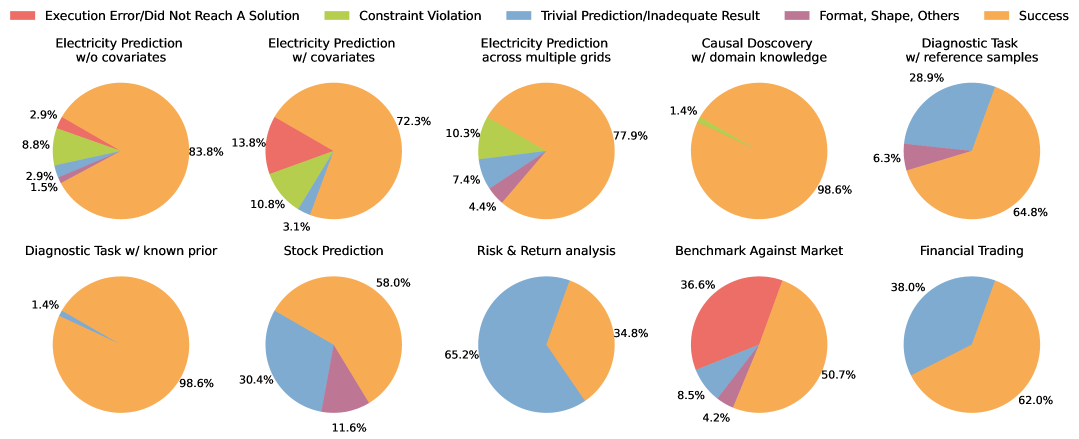
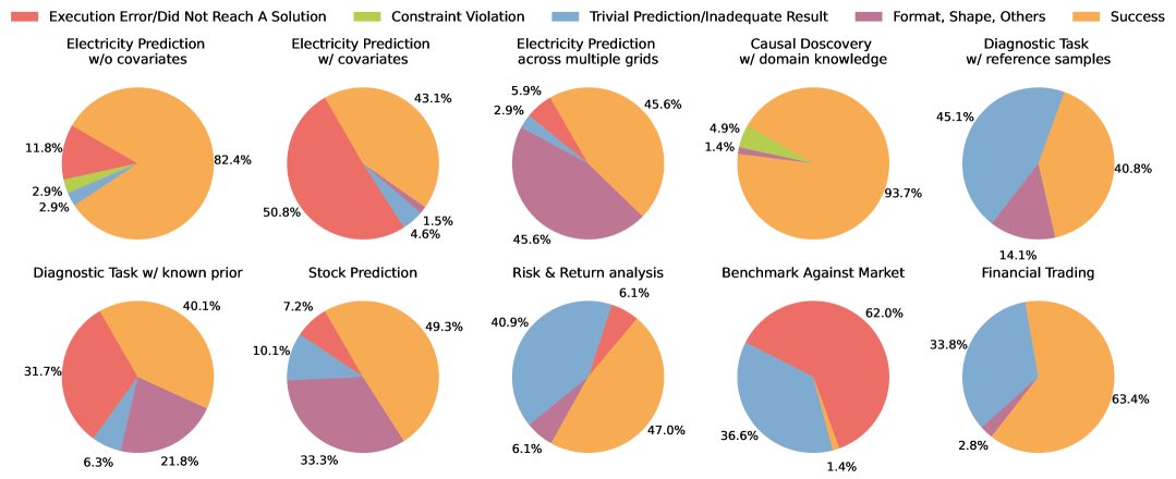
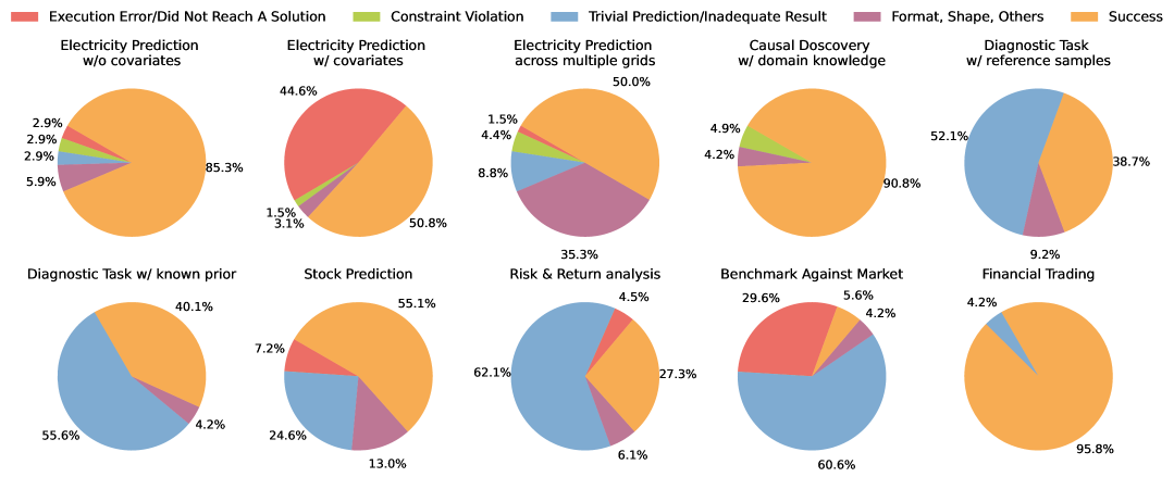
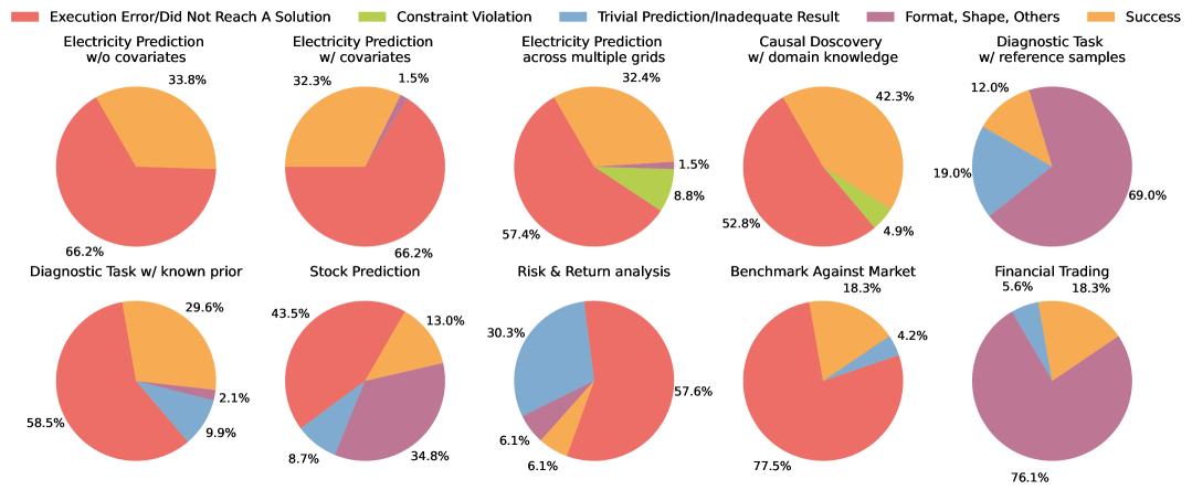
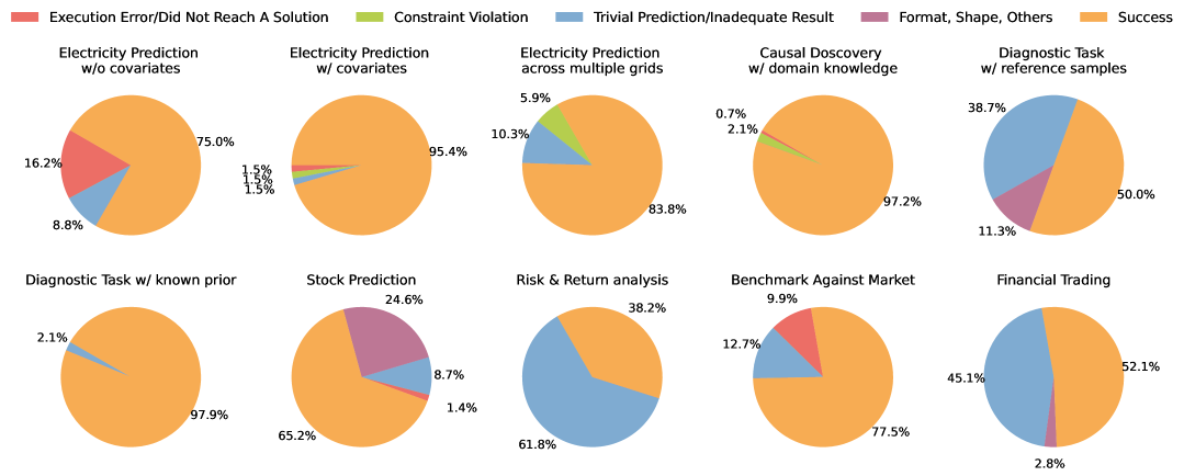
Beyond GPT-4o, we extend our error analysis to other representative models, whose detailed error distributions are visualized in Figures 8–14. While Claude-3.5 generally performs well, it exhibits a noticeable proportion of constraint violation errors in electricity prediction tasks, suggesting challenges in handling numerical constraints embedded within the input. Despite the complexity of financial trading tasks, Llama-3.1 performs competitively relative to other models—particularly notable given its open-source nature. In contrast, Gemini-2.0 and Codestral show a high incidence of execution errors across nearly all task categories, indicating limited suitability for structured, multi-step time series reasoning. DeepSeek-R consistently avoids execution failures and maintains a relatively high success rate across tasks.
Appendix C CodeAct System Prompt Template
Appendix D Refinement Solution Path
Box D illustrates the solution refinement trajectory of Deepseek-R. Execution feedback from the CodeAct Python interpreter enabled the model to revise its output twice—first to address a syntax error due to a missing closing parenthesis, and second to resolve an import error. As shown in Figure 6, Deepseek-R consistently requires more interaction turns than other models. A closer examination reveals that this behavior stems from the lack of a proper stopping mechanism: although a correct solution was reached by turn 3, the model continued executing redundant steps in turns 4 and 5. Notably, Deepseek-R also incorporates explicit inline comments such as # Total pairs: 5*4=20, top 20% is 4 pairs to document its intermediate reasoning steps, contributing to its overall performance strength.
Appendix E Casual Discovery Data Generation Prompt
Now you are a Time series data scientist, please help me to write the code to generate some synthetic data in real world Time series domain, you should save the data into "*/data.csv":
Now suggesting you should construct a series data based on a relation matrix and the correlation ratio for different influence factor, you should notice the following points,for time step I want you to generate 500 time steps:
1. data correlation: the multi variable should be correlated, sample: which A first influence B, then B have influence on C or D, there should be some time delay, as the influence on other staff needs time.
2. data trend: there should be some trend in the data, like the data is increasing or decreasing.
3. data: seasonality there should be some seasonality in the data, like the data is periodic.
4. data noise: the noise should be added to the data, as the real world data is not perfect.
5. data background: the data should have some real world background, you should first think about different real world data, and provide a description for the variable and time series data, then generate the data using the code. CoT Sample: Q: Approximate Relation Ratio: 0.5 Relation Matrix:
-
•
A influences B and D, and itself.
-
•
B influences D, and itself.
-
•
C influences B and D, and itself.
-
•
D influences only itself.
variable size: 4 A: Scenario: Sales Data of a Chain of Stores Over Time Let’s assume we are generating synthetic data,the variable size for the data is 4. for the daily sales of multiple stores across a chain, the sales numbers are influenced by:
1. Advertising (A): The level of advertising spend directly impacts the sales of each store. After a delay, this starts influencing sales. 2. Sales (B): The sales numbers for each store are influenced by both the advertising and local seasonal events. 3. Economic Factors (C): Broader economic trends, like GDP growth or unemployment rates, also impact sales. These factors show a delayed and more subtle influence over time. 4. Customer Sentiment (D): Customer sentiment affects the sales of specific products in each store and is influenced by both advertising and broader economic factors.
Seasonality: Sales experience periodic seasonal trends, with peaks around the holidays and lower numbers during off-seasons.
Trend: There is a general increasing trend in sales as the chain expands.
Noise: Random noise is added to mimic real-world data fluctuations.