Testing the assumptions about the geometry of sentence embedding spaces:
the cosine measure need not apply

Abstract

Transformer models learn to encode and decode an input text, and produce contextual token embeddings as a side-effect. The mapping from language into the embedding space maps words expressing similar concepts onto points that are close in the space. In practice, the reverse implication is also assumed: words corresponding to close points in this space are similar or related, those that are further are not.

Does closeness in the embedding space extend to shared properties for sentence embeddings? We present an investigation of sentence embeddings and show that the geometry of their embedding space is not predictive of their relative performances on a variety of tasks.

We compute sentence embeddings in three ways: as averaged token embeddings, as the embedding of the special [CLS] token, and as the embedding of a random token from the sentence. We explore whether there is a correlation between the distance between sentence embedding variations and their performance on linguistic tasks, and whether despite their distances, they do encode the same information in the same manner.

The results show that the cosine similarity – which treats dimensions shallowly – captures (shallow) commonalities or differences between sentence embeddings, which are not predictive of their performance on specific tasks. Linguistic information is rather encoded in weighted combinations of different dimensions, which are not reflected in the geometry of the sentence embedding space.

Testing the assumptions about the geometry of sentence embedding spaces:
the cosine measure need not apply

Vivi Nastase¹  and Paola Merlo^{1,2 1}Idiap Research Institute, Martigny, Switzerland ²University of Geneva, Swizerland vivi.a.nastase@gmail.com, Paola.Merlo@unige.ch

1 Introduction

Projecting words and larger pieces of text into an $n$-dimensional space allows us to map linguistic objects into a well-defined mathematical space, with specific metrics and operations. Building this projection relies on equating word similarity in language with closeness between their corresponding vectors in the embedding space, that is, the embedding space is smooth Bengio et al. (2013). The smoothness of the embedding space comes with several assumptions: similar or related words or sentences will be projected to points that are close in the space, and words or sentences corresponding to points that are close in the space are similar or related. Distance or similarity metrics in this space are the basis for the functioning of all current LLMs and their applications, and understanding the topology of the embedding space can bring insights both into the successes and also the failures of these models.

Analysis of the embedding spaces of the tokens through similarity measures have revealed that the spaces of many LLMs are anisotropic, with most words appearing in a narrow cone in this space, thus making distance metrics less informative Timkey and van Schijndel (2021); Cai et al. (2021). These analyses are shallow: each dimension of these vectors is treated independently of the other dimensions. The dimensions may encode some information at a shallow level – e.g. length, or extreme word frequencies within the sentence Nikolaev and Padó (2023b); sentence structure through the words’ relative positions Manning et al. (2020) – but they do not correspond to linguistic features such as phrase type, or semantic role. The interplay among embedding dimensions is complex, as each can contribute to various linguistic features in different measures Bengio et al. (2013); Elhage et al. (2022). This implies that the level at which words and sentence embeddings share features is not at a level that the cosine metric can detect. This explanation may also shed light on the apparent contradiction between the word embedding space being anisotropic Mimno and Thompson (2017); Timkey and van Schijndel (2021); Cai et al. (2021) while word embeddings still leading to good results on a variety of NLP tasks (e.g. Mercatali and Freitas (2021); Bao et al. (2019); Chen et al. (2019)).

We present an investigation of sentence embeddings and show that the geometry of their embedding space is not predictive of their relative performances on a variety of tasks. We consider four pretrained models from the BERT family . For each model, we study and compare three variations of sentence representations: the averaged token embeddings, the embedding of the special [CLS] token, and a random token embedding.

While the vocabulary is finite, the sentences in a language are not. We therefore study the embedding space of sentences by comparing variations of representations for the same sentence, which should (theoretically) be very close as they should contain the same information. For this analysis, we start with the commonly used method –the cosine similarity– and establish how close these representation variations are on a dataset of sentences extracted from the ParaCrawl corpus Bañón et al. (2020) (Section 2.5). In the next step, we test these sentence representations on the FlashHolmes benchmark Waldis et al. (2024), which contains morphological, syntactic, semantic, discourse and reasoning tasks, and test whether embeddings that are close in the embedding space lead to similar performance on linguistic tasks (Section 3). Finally, we mine for sentence structure information, and test whether this kind of information is encoded consistently across the three representation variations of a sentence (Section 4).

The results show that closeness in the embedding space is not predictive of closeness of performance. In particular, for RoBERTa, all representation variations of a sentence are close in the embedding space, but their performance on the FlashHolmes tasks are very different. For Electra and DeBERTa, the S_CLS  representations are almost orthogonal to the S_AVG  representations, while having very close performance on the FlashHolmes tasks, and on deeper probing for syntactic structure.

These seemingly contradictory results between distance in the embedding space and performance on various tasks support the view that the geometry of the embedding space is not a good proxy for investigating shared information among sentence embeddings. We discover linguistic features encoded through deeper combinations of weighted dimensions. Our work sheds lights on the embedding space, how linguistic information is encoded in embeddings and that cosine similarity is a shallow metric that does not provide information about (deep) shared features among words or sentences.

2 Sentence representation comparisons in the embedding space

We investigate the embedding space of sentences, and whether the common assumption – that close points correspond to textual units that are similar – is true for sentence representations.

2.1 Sentence representations

Averaged token embeddings: S_AVG

The representation obtained by averaging a sentence’s tokens (without the special [CLS] and [SEP] tokens) is frequently used as the sentence’s embedding (Nikolaev and Padó, 2023a). This representation benefits from the fact that the learning signal for transformer models is stronger at the token level, with a much weaker objective at the sentence level – next sentence prediction (Devlin et al., 2019; Liu et al., 2019), sentence order prediction (Lan et al., 2019).

The embedding of the special [CLS] token: S_CLS

This representation is most commonly used after fine-tuning for specific tasks such as story continuation (Ippolito et al., 2020), sentence similarity (Reimers and Gurevych, 2019), alignment to semantic features Opitz and Frank (2022).

The embedding of a random token: S${}_{T_{rand}}$

Using this as the sentence’s representation can reveal how much contextual information each token embedding contains.

We investigate these three variations of representing sentences in four pretrained transformer models: BERT, RoBERTa, DeBERTa, and Electra. BERT is the baseline transformer model. RoBERTa is a variation of BERT with optimized training, BPE tokenization, dynamic masking and without a next sentence objective Liu et al. (2019). DeBERTA is another variation that introduces disentangled attention and an optimized mask decoder training He et al. (2021). Unlike BERT, RoBERTa and DeBERTa, Electra is not a masked language model, rather implements a replaced token recognition model, predicting whether a token in the input was produced by a generator model Clark et al. (2020). Electra also outperforms XLNet Yang et al. (2019) and MPNet Song et al. (2020).The differences in the training regime and architecture of the models are reflected in the relative position of the embeddings in the embedding space (Section 2.5).

2.2 Analysis of the embedding space

Our investigation starts from shallow analyses based on the cosine metric between variations of sentence embeddings, tests these embeddings on a benchmark covering different NLP tasks, and probes for shared syntactic information, to establish whether closeness in the embedding space means close performance on NLP tasks.

We first use the cosine metric to quantify how close the tokens in a sentence are to each other (Section 2.4). According to the properties of the embedding space, this provides information about how similar the tokens are. Considering that most tokens in a sentence are not actually similar, and that the token embeddings are contextual, the cosine similarity rather quantifies how much contextual information these embeddings share.

We then use the cosine metric to quantify the distance between the three sentence representation variations (Section 2.5). Since they represent the same sentence, S_AVG  and S_CLS  encode the same information, and the embedding space assumption dictates that they be close in the embedding space. S${}_{T_{rand}}$, as the encoding of only one token, encodes less information about the sentence, and is expected to be further apart in the embedding space from both S_AVG  and S_CLS. We test whether these expectations are met.

In the third step, we use each variation of a sentence representation to solve the FlashHolmes linguistic tasks. The goal is to verify whether relative distances in the embedding space – quantified in the previous step – are reflected in the relative performance of the three sentence embedding variations on the benchmark (Section 3).

Finally, we test whether the three sentence representation variations all encode information about the chunk structure of a sentence, and if they do, whether it is encoded in the same way (Section 4).

2.3 Data

The dataset consists of 1000 sentences in six languages (English, French, German, Italian, Romanian, Spanish) extracted from the parallel ParaCrawl corpus Bañón et al. (2020) (the datasets are not parallel). Each sentence is represented through the three representation variations.

2.4 Contextual information in token and word embeddings

For each sentence $s$ in the dataset, we compute the cosine similarity between the embeddings of every pair of tokens and every pair of words. The density histogram plots are shown in Figure 1. For BERT, the similarities among the token representations have a wider distribution, while they become tighter and centered on a higher mean for the optimized BERT variations, RoBERTa and DeBERTa, and for Electra. The word embeddings – as averages of their token representations – follow similar trends. These results show that with the changes in the models (relative to BERT), tokens and words within the same sentence become closer in the embedding space. According to the assumption that close points correspond to similar words and vice-versa, we must conclude that the optimizations over the BERT base model lead to more sharing of contextual information among the words in a sentence.

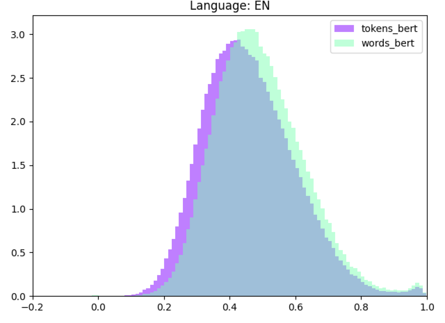
BERT	RoBERTa
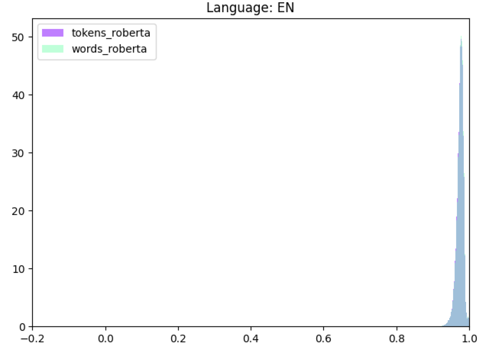
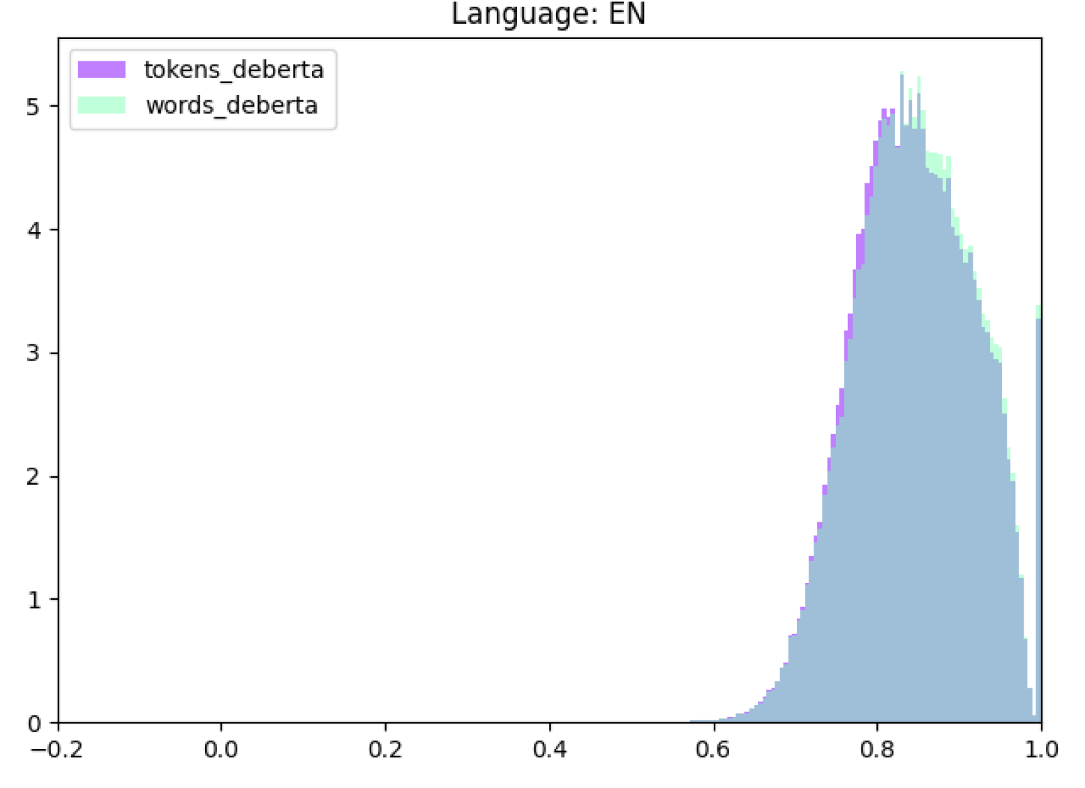
DeBERTa	Electra

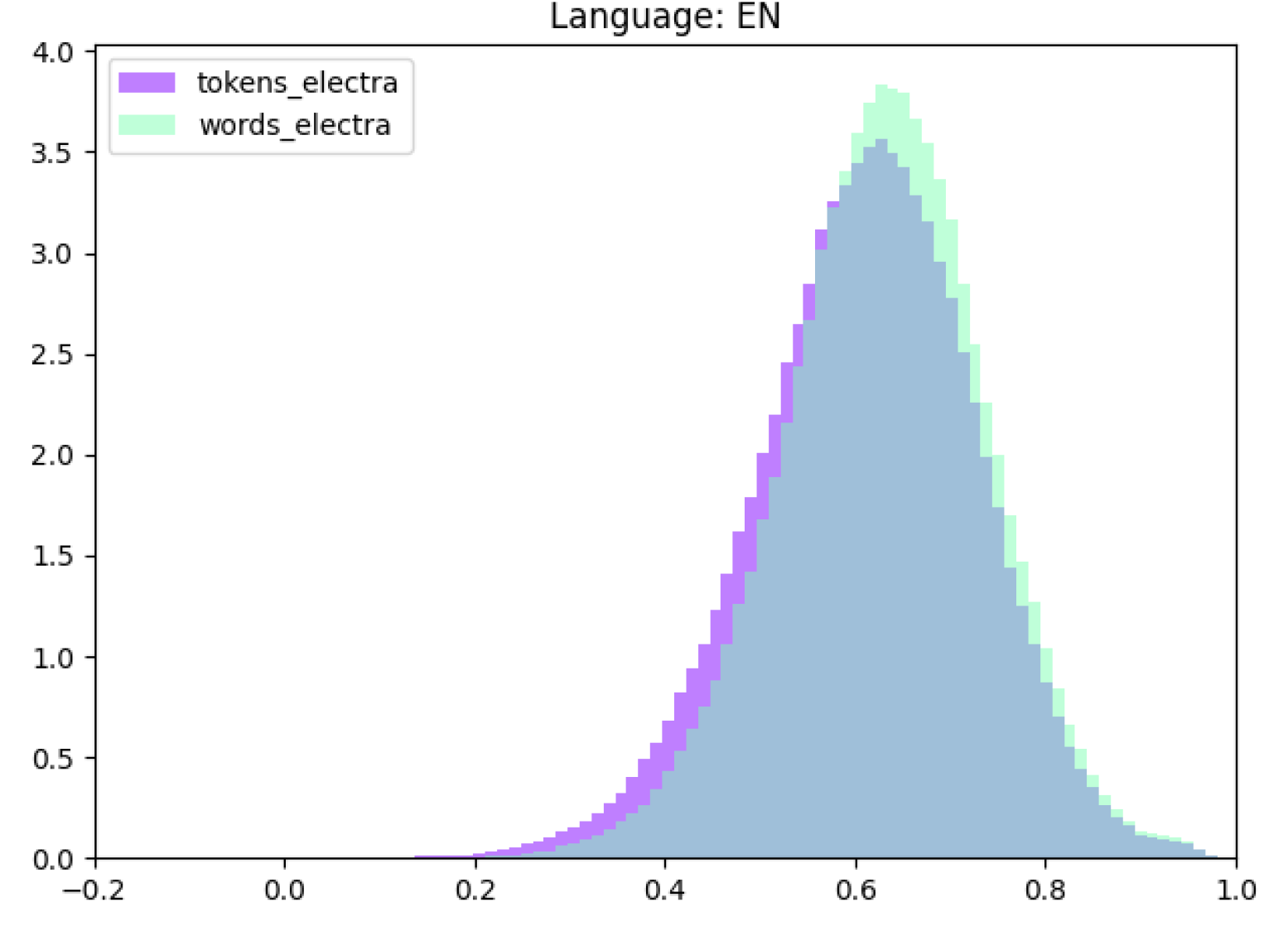
Figure 1: Histograms of cosine similarities for words and tokens in 1000 English sentences (results for French, German, Italian, Romanian and Spanish in appendix). The y-scales are different for each subplot for better visualization.

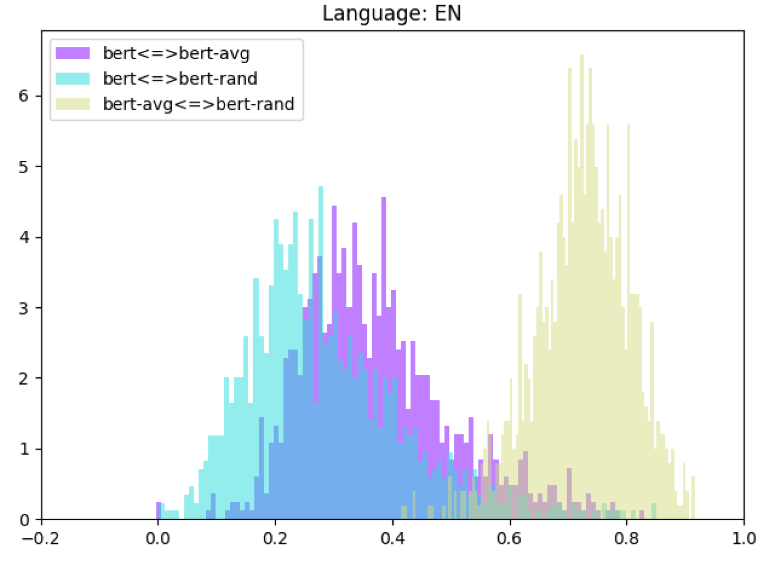
BERT	RoBERTa
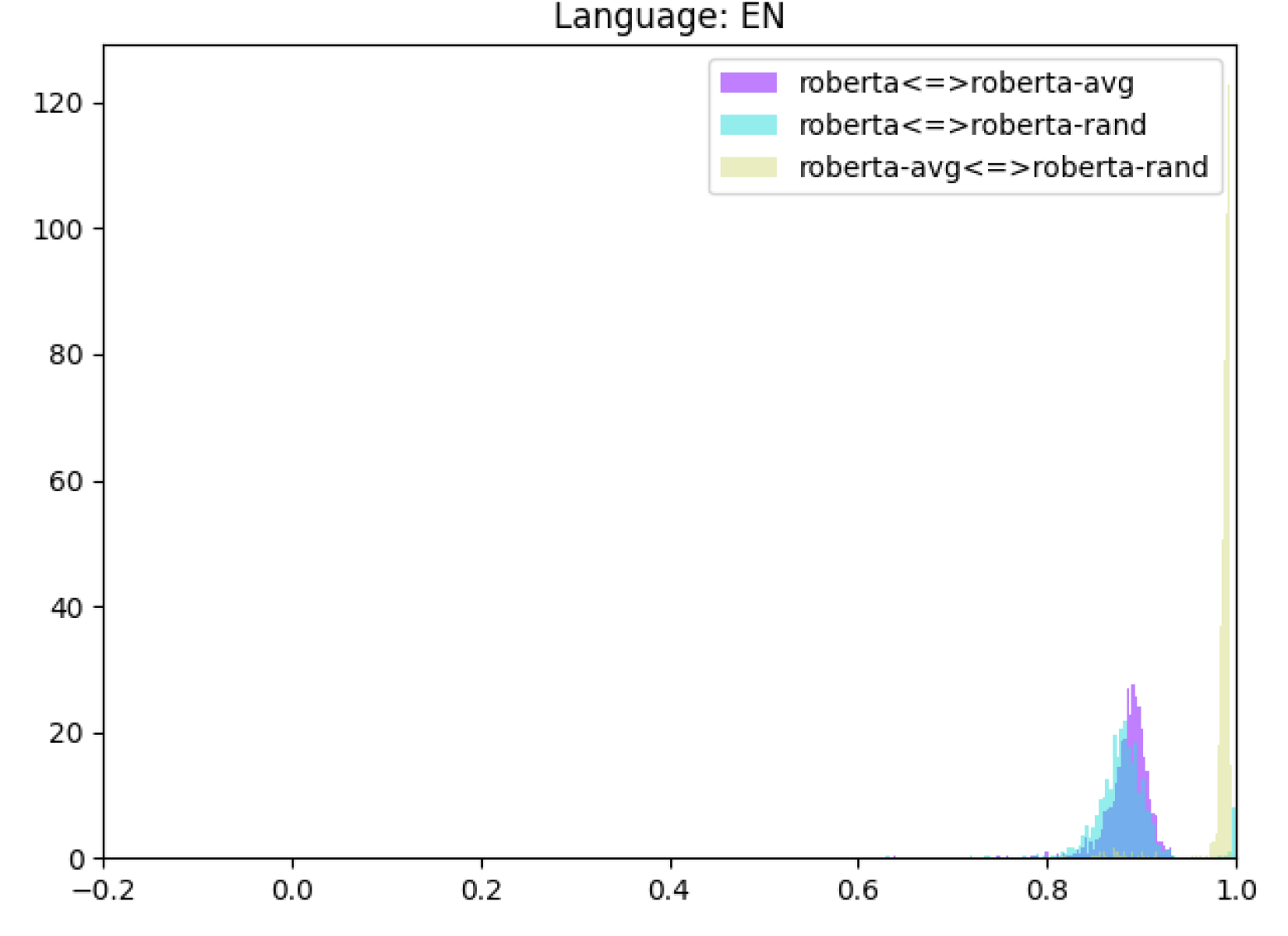
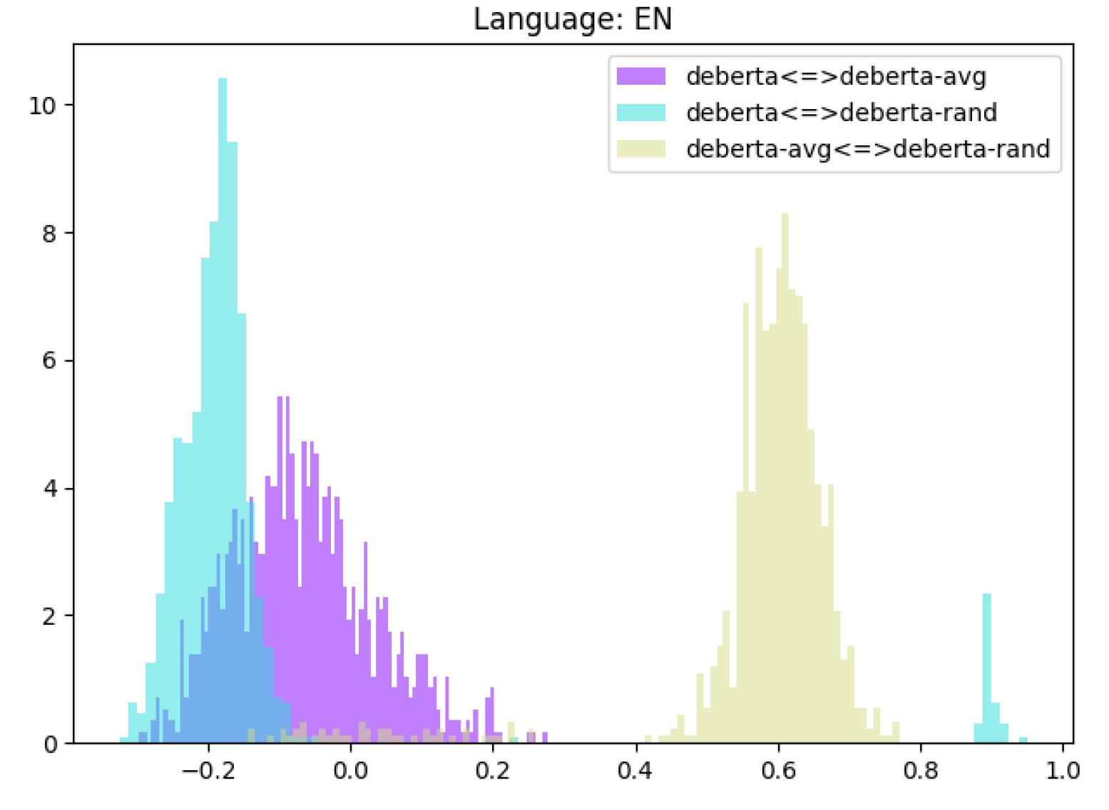
DeBERTa	Electra

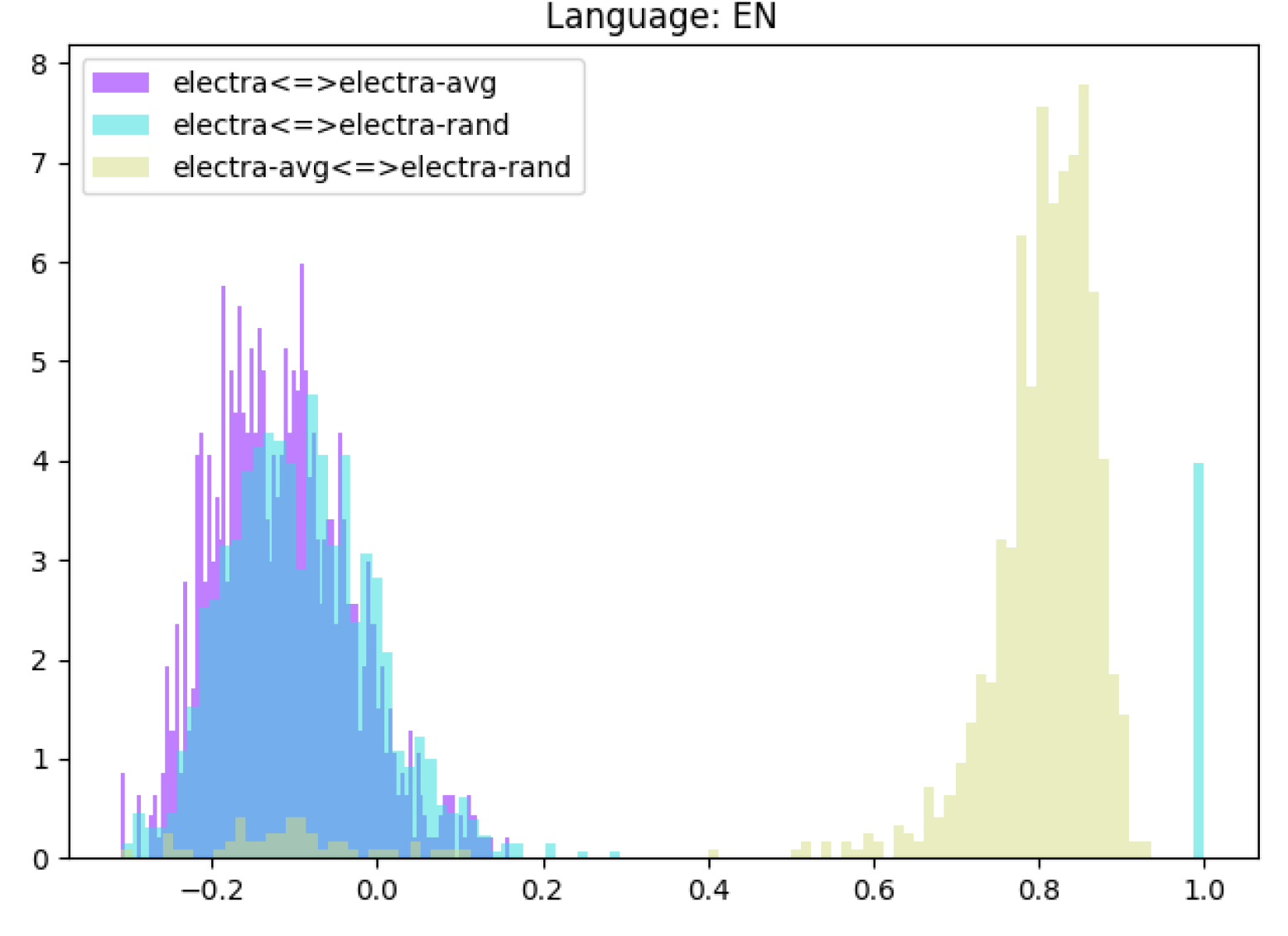
Figure 2: Histograms of cosine similarities computed for 1000 English sentences (results for French, German, Italian, Romanian and Spanish in appendix). In yellow are the distances between S_AVG  and S${}_{T_{rand}}$, in blue the distances between S_CLS  and S${}_{T_{rand}}$, and in purple the distances between S_CLS  and S_AVG. The y-scales are different for each subplot for better visualization.

2.5 Distance between sentence representation variations in the embedding space

The next step is an analysis of the distance between the three types of embeddings —token (S${}_{T_{rand}}$), averaged token (S_AVG), sentence (S_CLS)— for several models from the BERT family. For each sentence $s$ in the dataset, we compute the cosine between every pair of representations S_AVG($s$), S_CLS($s$) and S${}_{T_{rand}}$($s$). Figure 2 shows the histograms of these comparisons.This analysis also shows how the sentence representations change with the different training regimes and set-ups of the considered models.

For all models, S_AVG  are very close to S${}_{T_{rand}}$, adding support to the observation from Section 2.4, that tokens encode much contextual information. The holistic sentence embeddings S_CLS  are quite dissimilar from both S_AVG  and S${}_{T_{rand}}$  for all models except for RoBERTa. The optimized training of RoBERTa has the effect of bringing all variations of the sentence embeddings closer together. It is interesting to note that S_CLS  are almost orthogonal to S_AVG  and S${}_{T_{rand}}$  for both DeBERTa and Electra. Following the assumption of the smoothness of the embedding space, this may indicate that the holistic S_CLS  embeddings encode different types of information than the contextual embeddings. We will test this in the next sections.

3 Sentence representation comparisons on linguistics tasks

The previous analysis has shown that token embeddings encode much contextual information, and they, and the averaged token embeddings, are dissimilar from the embeddings of the special [CLS] token. This section shows experiments that investigate whether the similarities or differences noted in the embedding space analysis are reflected in their relative performances.

3.1 Dataset and code

We use the FlashHolmes benchmark Waldis et al. (2024) to test the three embedding types. There are 216 tasks in morphology, syntax, semantics, discourse and reasoning, code to test new models, and a leaderboard for comparisons. The input of a task is obtained from the specified model, and the output is predicted using a classifier probe implemented as a linear NN layer. The results on these tasks will help determine what kind of information the three types of embedding encode.

3.2 Performance comparisons

Figure 4 presents a summary of the performance of the different sentence representation methods for each task, and on the task averages. The first four bar groups show the number of times each of the three sentence representation methods (represented as different shades of the model colour) has achieved the best performance for that model. The fifth group shows the number of times each sentence variation for each model has had the best overall performance. The sixth panel shows these statistics as averages over all tasks.

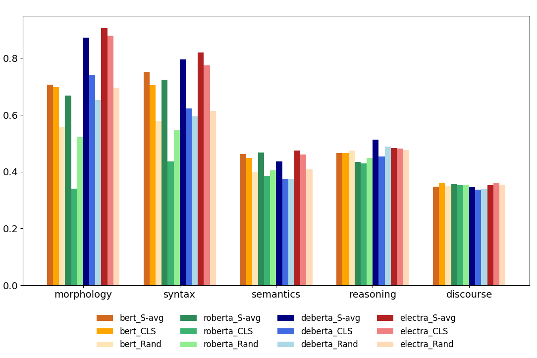
Figure 3: Comparison of embedding variations through average performance on the FlashHolmes benchmark

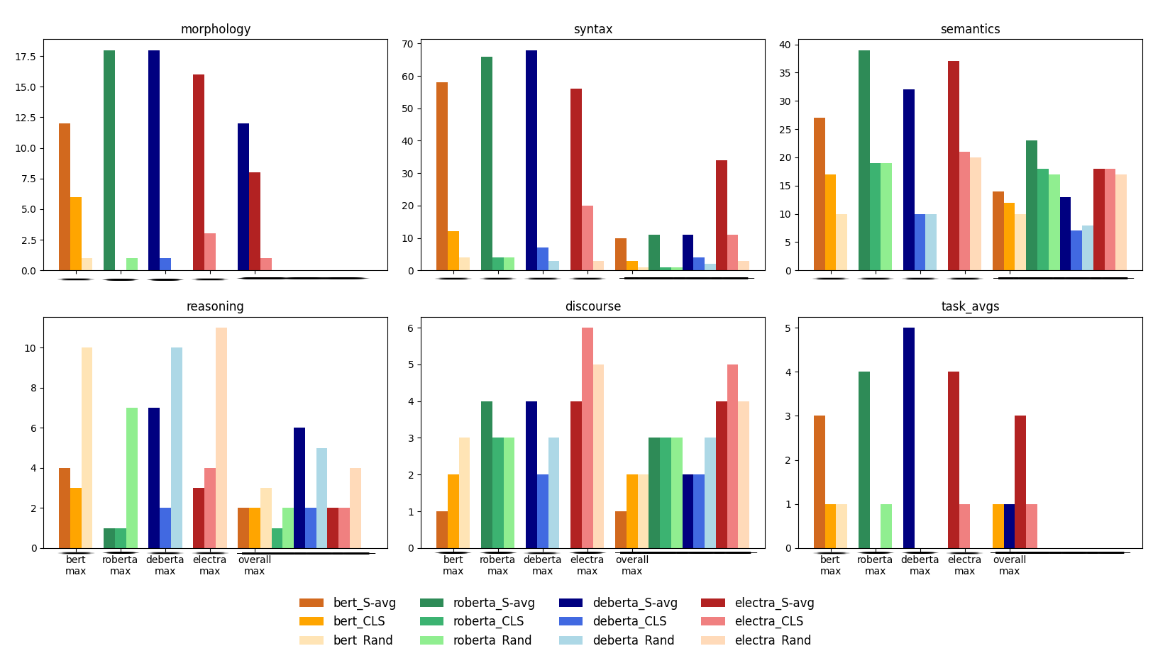
Figure 4: Statistics on the best sentence representation for each transformer, and overall for each task. The y-axis is the count of tasks for which a method performs best. For each transformer, we count the methods that performed best among the transformer’s variations. If all variations have the same score, we count them only if they match the highest overall scores for the task.

On morphology, syntax and semantics the S_AVG  has most frequently the highest performance for all models, while for reasoning and discourse S${}_{T_{rand}}$  is often the best. However, the results in Figure 3 show little variation in the results on the reasoning and discourse tasks, indicating that probably all results are close to the tasks baseline. For the morphology, syntax and semantics tasks, the performance of Electra’s S_AVG  and S_CLS  sentence representations are very close in terms of average performance, while S${}_{T_{rand}}$is much lower. This seemingly contradicts the analysis in Section 2.5 which shows that S_AVG  and S_CLS  representations are almost orthogonal, while S_AVG  and S${}_{T_{rand}}$  are very close. This supports the hypothesis that the geometry of the embedding space is not informative about the linguistic properties encoded by the embeddings. There can be an alternative explanation for the close performance of S_AVG  and S_CLS: they encode the same information, but in different ways. We explore this in the next section.

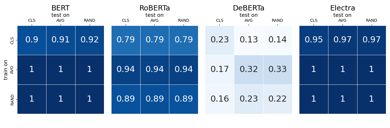
Figure 5: Comparison between models using S_AVG, S_CLS  and S${}_{T_{rand}}$  in detecting the sentence chunk structure in terms of average F1 scores over three runs. Detailed results in table 6 in the appendix.

S_AVG  and S_CLS  embeddings have high and close performance for most task types.Compared with the analysis of the embeddings as vectors in the embedding space, this result is unexpected, as for Electra and DeBERTa in particular, the S_CLS  and the S_AVG  embeddings are almost orthogonal. Not only these embeddings have similar performance, but even for variations of the same task S_AVG  gives best results for one task, and S_CLS  gives best results for the other. For RoBERTa, where the cosine similarity between these two variations is very high, their relative performance is very different.

4 Probing for structure

The previous experiments on a variety of morphological, syntactic, semantic, discourse and reasoning tasks within the FlashHolmes benchmark show very close performance on the S_AVG  and S_CLS  variations. In light of the analysis of the relative position of embeddings in the embedding space, these results are surprising: for Electra and DeBERTa in particular, the two representations seem to be almost orthogonal (see Figure 2). An explanation could be that the same type of clues necessary to solve these tasks is encoded in different manners in the two types of representations. We test whether this is indeed the case, by focusing on sentence structure. Sentence structure is complex, relying on clues about phrase boundaries and phrase properties. We test whether information about sentence structure can be detected in the three sentence representation variations, and whether it is encoded in a similar manner. For this we use the approach of Nastase and Merlo (2024), who have shown that some types of structural information – noun, prepositional, or verb phrase (chunks) structure – is recoverable from sentence representations. We use their code and data to investigate the sentence representations . Experiments that use the training and test data encoded using the same representation type will reveal whether the targeted sentence structure is identifiable. Cross-representation experiments – using the training data encoded with one type of representation, and the test data encoded with the other two types – will show whether the necessary information do detect structure is encoded in the same way.

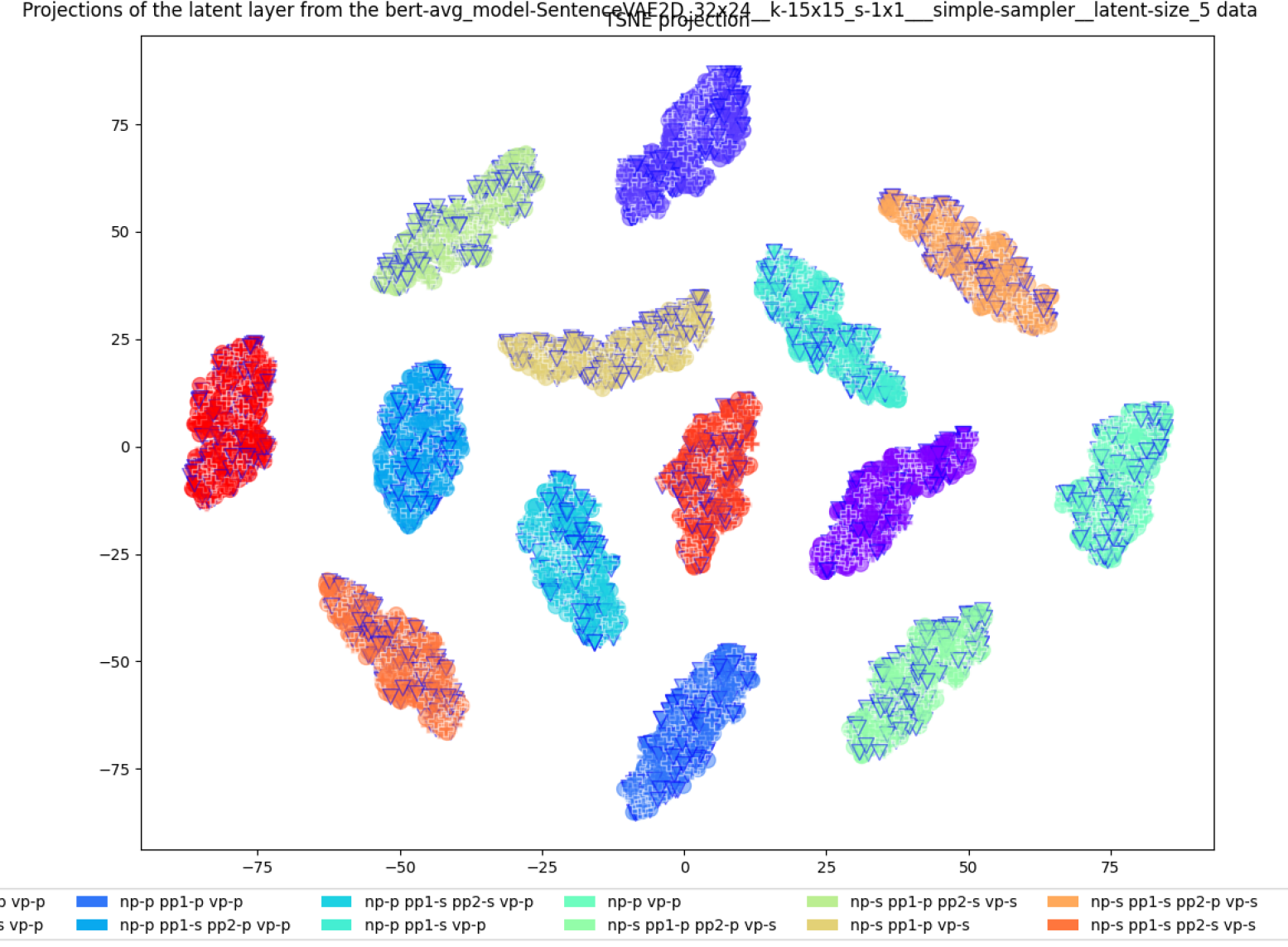
BERT	RoBERTa
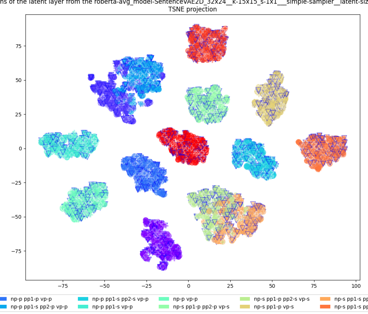
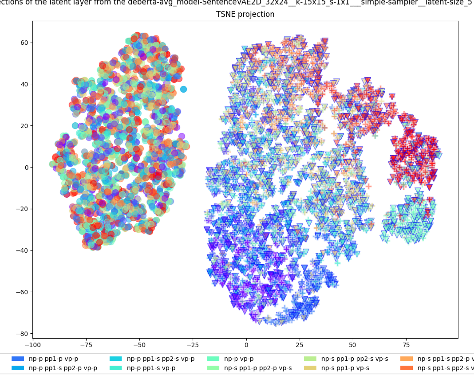
DeBERTa	Electra

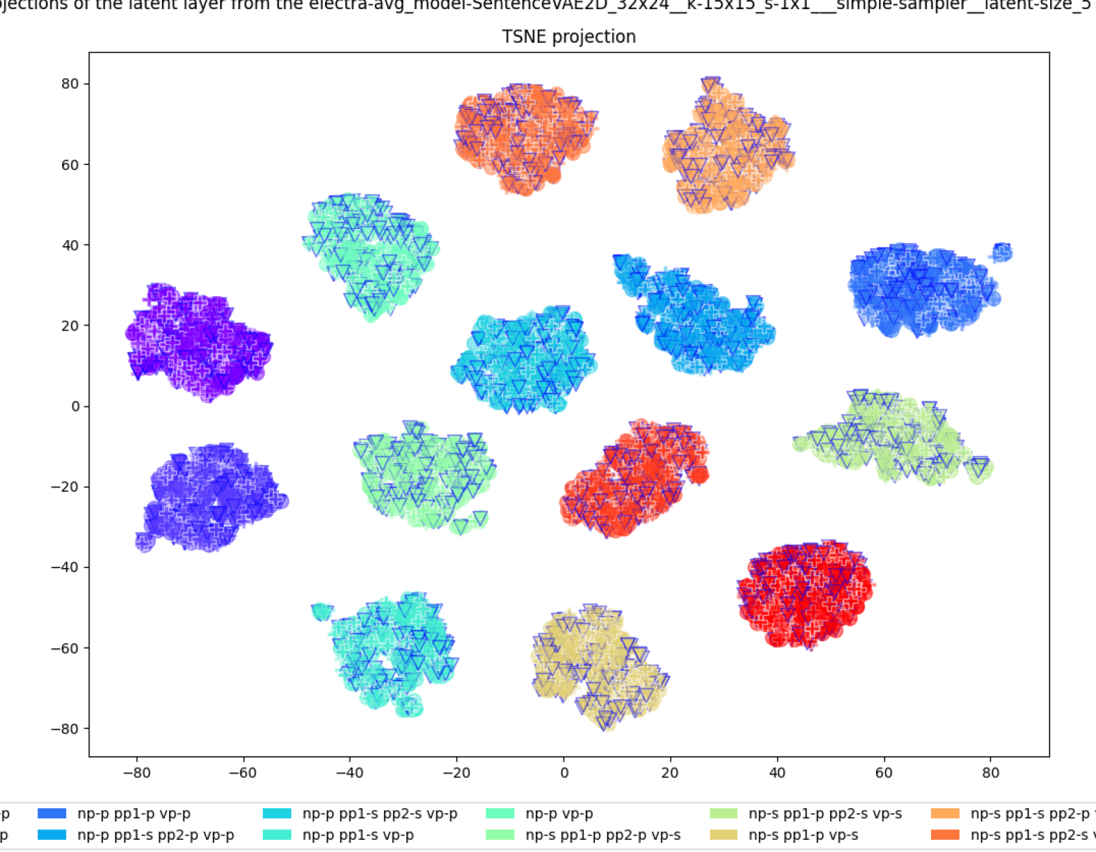
Figure 6: Comparison between models using S_AVG  ($\bigcirc$), S_CLS  ($\bigtriangledown$) and S${}_{T_{rand}}$  ($+$) in detecting the sentence chunk structure. tSNE plots of the latent layer vectors of the training data represented using S_AVG , S_CLS  and S${}_{T_{rand}}$, obtained from a model trained on the S_AVG  representation. The latent layer vectors are expected to encode the targeted information, i.e. the chunk structure. We note very sharp clusters for BERT and Electra

4.1 Dataset and code

The dataset

consists of English sentences with the syntactic pattern np (pp₁ (pp₂)) vp, where each np, pp₁, pp₂, vp can be in the singular or plural form, and the subject (np) always agrees with the verb (vp). There are 4004 sentences evenly split across the 14 chunk patterns. An instance is built for each sentence as a triple $(in,out^{+},Out^{-})$, where $in$ is an input sentence with chunk structure $p$, $out^{+}$ is a sentence different than $in$ but with the same chunk structure $p$, and $Out^{-}$ is a set of $N_{negs}=7$ sentences each of which has a chunk pattern different from $p$ (and different from each other). The 4004 instances are split into train:dev:test – 2576:630:798.

The system

is a variational encoder-decoder. The encoder consists of a CNN layer that splits the input sentence embedding into layers of information, which it then compresses using a linear layer into a small latent representation. The decoder is a mirror image of the encoder, but unlike a regular variational auto-encoder, it does not reconstruct the input. Sentence embeddings have 768 dimensions, and are compressed on the latent layer to size 5. To encourage the sentence chunk structure to be encoded in the latent layer, each input $in$ will be decoded into $out^{+}$ – a different sentence but with the same chunk structure – using the $N_{negs}$ sentences with different structure than the input as contrastive examples. While the system receives a supervision signal – the correct output – it does not receive explicit information about a sentence’s structure. While there are 14 structure patterns in the data, each instance contains 7 randomly chosen negative instances. So with respect to the sentence structure, there is only indirect supervision.

4.2 Performance comparison

We apply this approach to the provided sentence data when using the S_CLS, S_AVG  and S${}_{T_{rand}}$  sentence representations. We present two perspectives of the performance: (i) in terms of F1 averages over three runs (how well does the system perform in building a sentence representation closest to the correct one) shown in Figure 5 and (ii) an analysis of the latent layer of the system, shown in Figure 6.

Despite high results on the syntactic and semantic Holmes tasks, detecting the chunk structure is not successful on the DeBERTa embeddings. This may be because of DeBERTa’s optimized training, with disentangled attention matrices and token embeddings with separate position and content sections, which leads to differently organized embeddings than BERT, RoBERTa and Electra. BERT and Electra in particular show very high results, with results on S${}_{T_{rand}}$  even higher than S_CLS.

For the purpose of determining whether the variations in sentence representation encode the same information in the same manner, we look at the cross-testing results – training on one representation, and testing on the others (Figure 5). Despite the differences revealed by the cosine similarity analysis, where for Electra the S_CLS  representations are almost orthogonal to S_AVG  and S${}_{T_{rand}}$, these experiments show that all three representations encode information about the chunk pattern in a sentence, and moreover, this information is encoded in the same manner. Additional support for this hypothesis comes from the analysis of the latent layer. Figure 6 show the tSNE projection of the latent representations obtained from a model trained using the S_AVG  sentence representations. After training on the training data represented with S_AVG, we pass through the encoder the sentences in the dataset encoded with all sentence representation variations, collect all latents and project them in 2D using tSNE.

The results on the task and the analysis of the latent vectors provide complementary views about whether structural information is encoded in the sentence embeddings. We may obtain high results on the task (choosing the sentence with the same structure) while for each sentence representation the vectors are mapped into a different area in the latent space. The tSNE plots show that in fact the different types of sentence representations are mapped onto shared regions. This is highly significant: it indicates that the clues based on which the structure is detected is encoded in a similar manner in all the three sentence representations, regardless of the differences among them we have noted during the previous experiments.

Nastase et al. (2024) have shown, through experiments on several languages, that sentence embeddings do not encode chunk structure as an abstraction, but rather linguistic clues – such as phrase boundaries and number information – that can be assembled into the chunk structure. Considering this, and the results in Figure 5 and the plots in Figure 6, this indicates that the S_AVG  and S_CLS  encode the information about phrase boundaries and number in the same manner and in the same location for BERT and Electra in particular.

5 Word and text representations in the embedding space

The evolution of the embedding space

Procedurally and scale-wise, we have come a long way from the first distributional models of language inspired by Harris (1954) and Firth (1957), with tens of thousands of symbolic dimensions computed over a small (relative to what is used today) corpus Schütze (1992).Symbolic dimensions are interpretable, but also brittle, and overlapping, and were tackled using clustering Pantel and Lin (2002); Blei et al. (2003), or dimensionality reduction Furnas et al. (1988); Landauer and Dumais (1997); Jolliffe (2002); Blei et al. (2003). Landauer and Dumais (1997)’s approach can be viewed as 3 layer neural network, but Bengio et al. (2003) first used a neural network to encode the probability function of word sequences in terms of the feature vectors of the words in the sequence. Pre-trained word embeddings, started with Mikolov et al. (2013b, a), have been shown to encode syntactic and semantic information, as regularities in the relative position of words in the low-dimensional vector space Ethayarajh et al. (2019). Currently, contextual embeddings are obtained with transformer-based models Vaswani et al. (2017). Models from the BERT family Devlin et al. (2019) produce token embeddings and sentence representations as the embedding of a special [CLS] token. Generative language models do not produce sentence embeddings as such, although approximations can be obtained using word definition-like prompts Jiang et al. (2024).

Embedding dimensions encode some linguistic information: shallow information about sentences Nikolaev and Padó (2023b), sentence-level information (Tenney et al., 2019), including syntactic structure – reflected as relative positions in the embedding space that parallel a syntactic tree (Hewitt and Manning, 2019; Chi et al., 2020). Deeper exploration through simple classification probes (consisting of one linear NN), has shown that predicate embeddings contain information about their semantic roles structure (Conia and Navigli, 2022; Silva De Carvalho et al., 2023), embeddings of nouns encode subjecthood and objecthood (Papadimitriou et al., 2021), and syntactic and semantic information can be teased apart Mercatali and Freitas (2021); Bao et al. (2019); Chen et al. (2019).

The geometry of the embedding space

The embedding space of tokens appears to be anisotropic Mimno and Thompson (2017); Timkey and van Schijndel (2021); Cai et al. (2021), which can adversely influence model training and fine-tuning. Anisotropy could be caused by a few dominant dimensions, that can skew the similarity profile of the space Timkey and van Schijndel (2021). However, the embedding space actually contains isotropic clusters and lower-dimensional manifolds that reflect word frequency properties Cai et al. (2021).

6 Discussion and Conclusions

The output of pretrained language models provide embeddings for individual tokens, and a holistic sentence embedding as the embedding of a special token. A sentence is often represented through the averaged embeddings of its tokens, or through this special token embedding. In the extreme, we could even use the embedding of a random token to represent the sentence. In this work, we explored how different, or similar, these three types of representations are, and what kind of information they encode. What we found is a complex picture. Shallow analysis through cosine similarity measures shows how distinct these three representations are, and how they change relative to each other from a baseline system (BERT) with various optimizations (RoBERTa), internal organization changes (DeBERTa) or changes in the training regimen (Electra) of the system. These shallow differences or similarities are not reflected in benchmarks on five types of NLP tasks, where seemingly orthogonal representations lead to very similar results on many tasks.

The close performance of the seemingly very distinct sentence representations raises another question: do they encode similar information in a similar manner, or the results come from exploiting different, or differently encoded, cues? Experiments in detecting a sentence’s chunk structure – the sequence of NP/VP/PP phrases and their grammatical number attributes – showed that in fact information relevant for reconstructing this structure is encoded in the same manner, as a system trained on one sentence representation has a very similar performance when tested on the other.

The experiments presented in this paper add to the complex picture of what kind of information the embeddings induced by pretrained transformer models encode, and how. The results show that embedding dimensions do not encode linguistic information superficially, rather linguistic features are encoded through more complex weighted combinations of features. Some of these are shared among all tokens in a sentence, and within the holistic sentence embedding.

7 Limitations

Synthetic data with 14 structure patterns

To study the deeper question of whether the different sentence embedding variations encode sentence structure the same way, we have used a synthetic dataset, with limited variation in sentence structure, expressed as a sequence of chunks, or phrases. In future work we plan to investigate what level of structure complexity can be recovered from these embeddings, and whether at some complexity level, differences among the embedding variations becomes apparent.

Raw output of transformer models

We have focused on four pretrained models from the BERT family, and analyzed their sentence embedding space through cosine similarity, solving tasks and detecting sentence structure. We have excluded from the related work and analysis sentence transformers, which fine-tune sentence embeddings for similarity. Our aim was to study the raw output of the transformer models, and understand the properties of the different types of embeddings they induce.

No generative language models

We focused on models form the BERT family because they explicitly induce sentence representations as the embedding of a special token, or they can be computed as averaged token embeddings. It was crucial for our experiments to have several sentence representation variations to compare. Generative models do not produce sentence embeddings. Representations approximating such representations have been induced using word definition-like prompts Jiang et al. (2024); Zhang et al. (2024). Our interest has been to study more fundamental properties of transformer-based models, rather than test the performance of sentence representation approximations.

Cosine similarity

We reported analyses in terms of cosine similarity which is the most commonly used in the training objective. The analysis in terms of euclidean distance did not provide additional insights, so it was not included.

Appendix A Words vs. token embedding similarities distribution

Figure 7 shows a comparison between the distribution of token and word similarities within the same sentence. A tighter distribution – as displayed by RoBERTa embeddings – indicates that all contextual embeddings are closer to each other, and thus encode more contextual information. BERT and Electra embeddings display distributions with larger standard deviation, indicating that there is more variation in the information encoded in the individual tokens and words. Electra token/word distances have a higher mean, indicating that these embeddings encode more contextual information than BERT ones. All distributions have a high spike close to 0. These pairs include punctuation and "suffix" tokens.

Lang	BERT	RoBERTa	DeBERTa	Electra
English
French
German
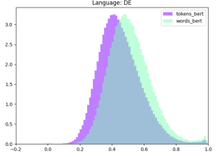
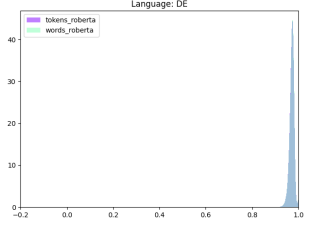
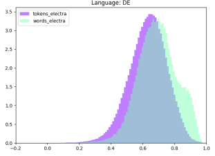
Italian
Romanian
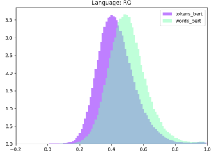
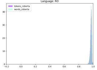
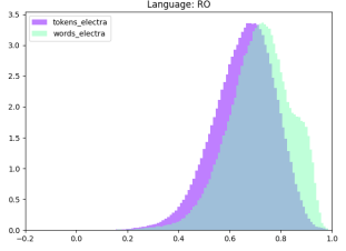
Spanish

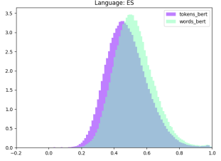
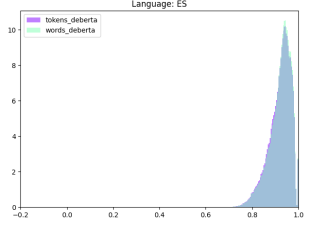
Figure 7: Cosine similarities histograms computed for words and tokens from 1000 English/French/German/Italian/Romanian/Spanish.

Appendix B Multilingual embeddings comparison

Lang	BERT	RoBERTa	DeBERTa	Electra
English
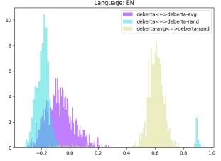
French
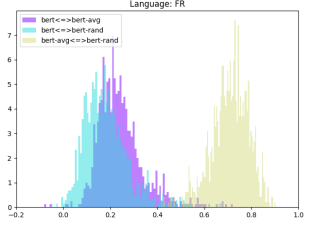
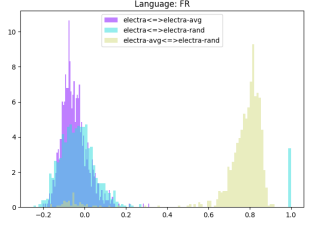
German
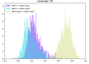
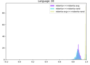
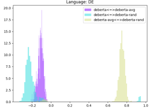
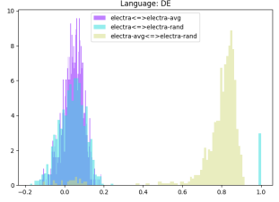
Italian
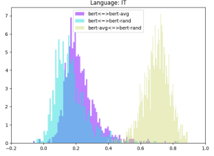
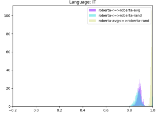
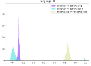
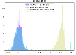
Romanian
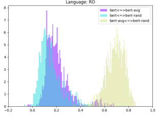
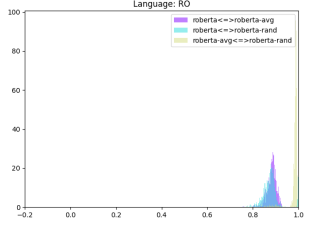
Spanish

Figure 8: Cosine similarities histograms computed for 1000 English/French/German/Italian/Romanian/Spanish sentences. In yellow are the distances between S_AVG  and S${}_{T_{rand}}$, in blue the distances between S_CLS  and S${}_{T_{rand}}$, and in purple the distances between S_CLS  and S_AVG.

Appendix C Task results

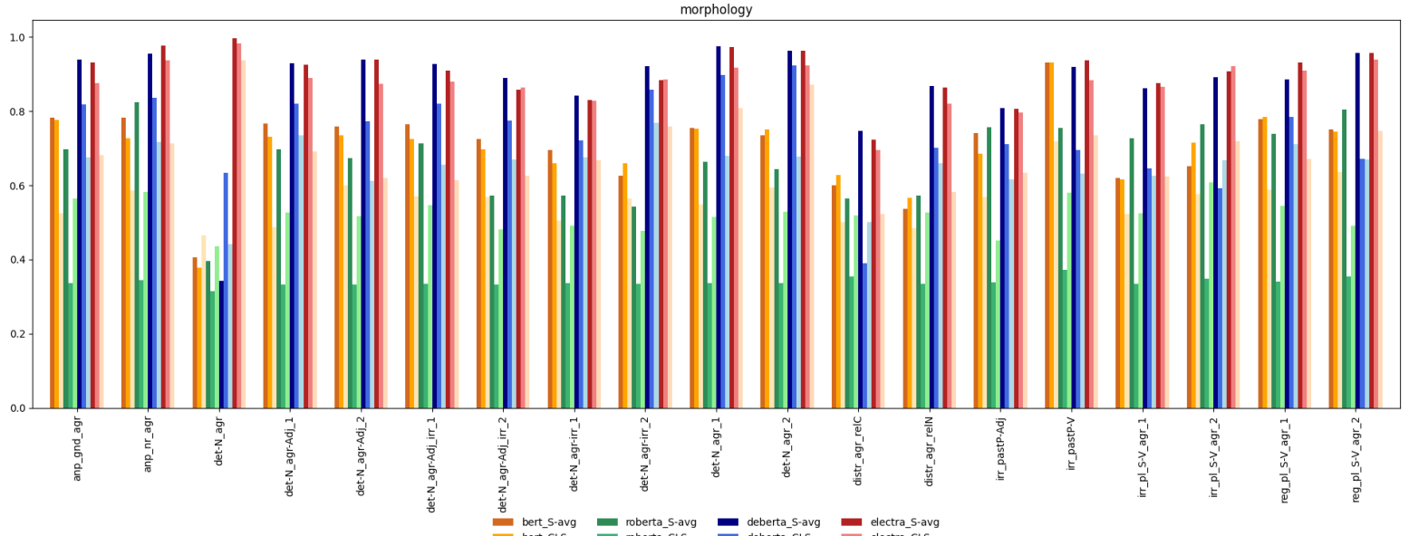
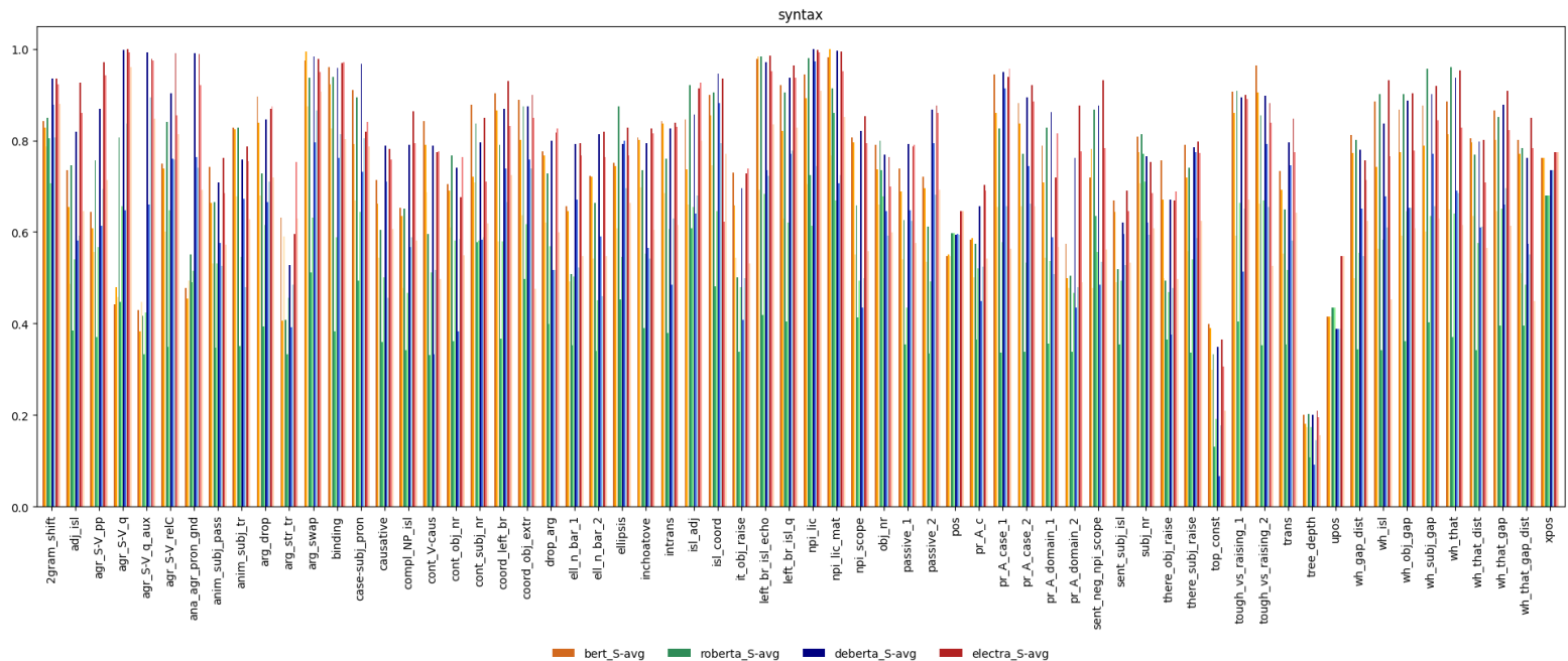
Morphology tasks Syntactic tasks Semantic tasks

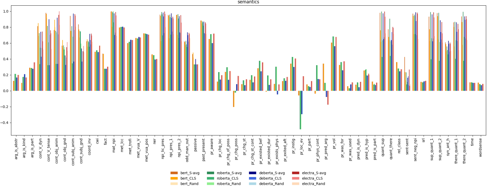
Figure 9: Detailed results on the FlashHolmes benchmark, on morphology, syntax and semantic tasks

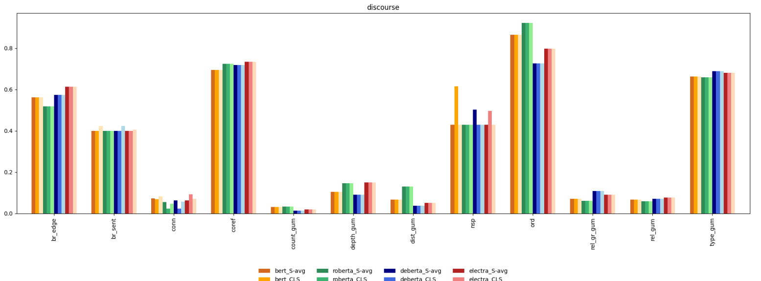
Discourse tasks Reasoning tasks

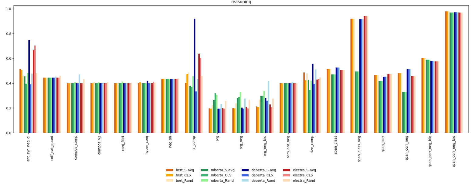
Figure 10: Detailed results on the FlashHolmes benchmark, on discourse and reasoning tasks

Data	BERT			RoBERTa			DeBERTa			Electra
	S-avg	CLS	Rand	S-avg	CLS	Rand	S-avg	CLS	Rand	S-avg	CLS	Rand
blimp-anaphor_gender_agreement	0.782	0.776	0.525	0.696	0.336	0.564	0.939	0.818	0.676	0.931	0.875	0.682
blimp-anaphor_number_agreement	0.782	0.727	0.586	0.825	0.345	0.582	0.954	0.835	0.717	0.977	0.937	0.712
blimp-determiner_noun_agreement_1	0.755	0.752	0.549	0.664	0.336	0.514	0.974	0.898	0.678	0.973	0.918	0.809
blimp-determiner_noun_agreement_2	0.736	0.75	0.594	0.644	0.336	0.529	0.963	0.922	0.677	0.963	0.924	0.873
blimp-determiner_noun_agreement_irregular_1	0.694	0.66	0.505	0.572	0.336	0.49	0.842	0.721	0.675	0.83	0.829	0.668
blimp-determiner_noun_agreement_irregular_2	0.626	0.66	0.565	0.542	0.334	0.476	0.922	0.857	0.768	0.884	0.885	0.758
blimp-determiner_noun_agreement_with_adj_2	0.759	0.735	0.601	0.673	0.333	0.517	0.938	0.773	0.611	0.939	0.873	0.620
blimp-determiner_noun_agreement_with_adj_irregular_1	0.765	0.725	0.57	0.713	0.334	0.546	0.927	0.82	0.656	0.909	0.879	0.613
blimp-determiner_noun_agreement_with_adj_irregular_2	0.725	0.698	0.568	0.573	0.333	0.481	0.889	0.775	0.670	0.857	0.864	0.627
blimp-determiner_noun_agreement_with_adjective_1	0.767	0.73	0.487	0.697	0.333	0.528	0.929	0.82	0.736	0.925	0.89	0.692
blimp-distractor_agreement_relational_noun	0.537	0.567	0.485	0.573	0.334	0.526	0.868	0.702	0.659	0.864	0.819	0.582
blimp-distractor_agreement_relative_clause	0.6	0.628	0.501	0.565	0.354	0.518	0.746	0.39	0.501	0.723	0.696	0.524
blimp-irregular_past_participle_adjectives	0.742	0.685	0.569	0.757	0.338	0.451	0.808	0.712	0.616	0.806	0.796	0.633
blimp-irregular_past_participle_verbs	0.932	0.931	0.718	0.754	0.372	0.58	0.92	0.695	0.633	0.936	0.884	0.736
blimp-irregular_plural_subject_verb_agreement_1	0.619	0.615	0.523	0.727	0.334	0.525	0.861	0.647	0.626	0.875	0.866	0.624
blimp-irregular_plural_subject_verb_agreement_2	0.651	0.716	0.577	0.764	0.349	0.608	0.892	0.591	0.667	0.908	0.922	0.720
blimp-regular_plural_subject_verb_agreement_1	0.779	0.785	0.588	0.739	0.341	0.544	0.885	0.785	0.711	0.93	0.909	0.672
blimp-regular_plural_subject_verb_agreement_2	0.75	0.746	0.637	0.804	0.354	0.49	0.957	0.671	0.670	0.957	0.938	0.747
zorro-agreement_determiner_noun-between_neighbors	0.407	0.378	0.466	0.395	0.315	0.435	0.343	0.633	0.442	0.996	0.983	0.937
average	0.706	0.698	0.559	0.667	0.339	0.521	0.871	0.740	0.652	0.904	0.878	0.696

Table 1: FlashHolmes morphology tasks results. In bold are the overall best results, and underlined are the results for the best performing variation for each transformer.

Table 2: FlashHolmes syntactic tasks results. In bold are the overall best results, and underlined are the results for the best performing variation for each transformer.

Data	BERT			RoBERTa			DeBERTa			Electra
	S-avg	CLS	Rand	S-avg	CLS	Rand	S-avg	CLS	Rand	S-avg	CLS	Rand
blimp-adjunct_island	0.735	0.655	0.487	0.746	0.384	0.539	0.818	0.581	0.592	0.925	0.861	0.646
blimp-animate_subject_passive	0.743	0.663	0.531	0.665	0.346	0.531	0.709	0.577	0.527	0.761	0.685	0.573
blimp-animate_subject_trans	0.827	0.824	0.678	0.828	0.351	0.546	0.759	0.673	0.479	0.787	0.755	0.628
blimp-causative	0.714	0.661	0.544	0.605	0.36	0.501	0.788	0.71	0.456	0.782	0.758	0.605
blimp-complex_NP_island	0.652	0.634	0.478	0.65	0.341	0.467	0.791	0.566	0.589	0.863	0.794	0.581
blimp-coord_str_constr_complex_left_branch	0.902	0.865	0.58	0.79	0.367	0.58	0.87	0.739	0.665	0.929	0.831	0.724
blimp-coord_str_constr_object_extraction	0.888	0.801	0.637	0.874	0.498	0.617	0.875	0.759	0.739	0.899	0.85	0.476
blimp-drop_argument	0.775	0.766	0.621	0.729	0.4	0.569	0.8	0.516	0.516	0.817	0.827	0.599
blimp-ellipsis_n_bar_1	0.656	0.645	0.492	0.508	0.352	0.503	0.792	0.67	0.522	0.794	0.767	0.548
blimp-ellipsis_n_bar_2	0.723	0.72	0.543	0.664	0.34	0.45	0.813	0.589	0.46	0.818	0.763	0.547
blimp-existential_there_object_raising	0.757	0.671	0.5	0.494	0.364	0.469	0.67	0.375	0.478	0.669	0.688	0.497
blimp-existential_there_subject_raising	0.791	0.718	0.558	0.74	0.336	0.54	0.785	0.774	0.587	0.797	0.772	0.624
blimp-expletive_it_object_raising	0.729	0.659	0.544	0.5	0.337	0.48	0.695	0.409	0.499	0.729	0.739	0.532
blimp-inchoative	0.806	0.801	0.698	0.736	0.39	0.552	0.793	0.565	0.542	0.825	0.815	0.604
blimp-intransitive	0.841	0.837	0.685	0.76	0.379	0.606	0.826	0.485	0.629	0.838	0.829	0.615
blimp-left_branch_island_echo_question	0.978	0.984	0.692	0.983	0.418	0.683	0.97	0.735	0.722	0.985	0.95	0.835
blimp-left_branch_island_simple_question	0.921	0.821	0.63	0.904	0.405	0.62	0.937	0.771	0.777	0.964	0.937	0.828
blimp-only_npi_scope	0.807	0.796	0.55	0.658	0.413	0.494	0.822	0.435	0.498	0.853	0.795	0.559
blimp-passive_1	0.738	0.689	0.541	0.625	0.355	0.434	0.791	0.648	0.624	0.787	0.791	0.576
blimp-passive_2	0.72	0.696	0.534	0.611	0.335	0.492	0.867	0.793	0.681	0.876	0.859	0.691
blimp-principle_A_c_command	0.583	0.586	0.5	0.574	0.365	0.52	0.657	0.448	0.525	0.702	0.69	0.541
blimp-principle_A_case_1	0.944	0.86	0.654	0.826	0.336	0.577	0.949	0.913	0.657	0.939	0.956	0.563
blimp-principle_A_case_2	0.882	0.836	0.657	0.771	0.338	0.532	0.894	0.744	0.662	0.921	0.886	0.657
blimp-principle_A_domain_1	0.788	0.708	0.544	0.828	0.356	0.536	0.862	0.588	0.507	0.719	0.816	0.567
blimp-principle_A_domain_2	0.575	0.499	0.478	0.505	0.339	0.468	0.762	0.434	0.479	0.877	0.775	0.49
blimp-principle_A_domain_3	0.64	0.649	0.495	0.524	0.335	0.493	0.839	0.533	0.515	0.877	0.82	0.548
blimp-principle_A_reconstruction	0.948	0.88	0.58	0.752	0.333	0.557	0.808	0.467	0.584	0.949	0.599	0.585
blimp-sentential_negation_npi_scope	0.719	0.781	0.477	0.867	0.634	0.556	0.876	0.484	0.534	0.931	0.783	0.561
blimp-sentential_subject_island	0.669	0.645	0.49	0.519	0.354	0.493	0.62	0.595	0.527	0.69	0.645	0.534
blimp-tough_vs_raising_1	0.907	0.86	0.592	0.908	0.404	0.663	0.893	0.513	0.651	0.899	0.891	0.671
blimp-tough_vs_raising_2	0.964	0.904	0.661	0.855	0.353	0.669	0.898	0.792	0.655	0.882	0.839	0.526
blimp-transitive	0.732	0.693	0.553	0.65	0.354	0.516	0.796	0.746	0.581	0.847	0.774	0.641
blimp-wh_island	0.886	0.742	0.563	0.901	0.342	0.583	0.836	0.679	0.609	0.931	0.766	0.452
blimp-wh_questions_object_gap	0.867	0.774	0.593	0.901	0.361	0.645	0.888	0.653	0.653	0.902	0.779	0.607
blimp-wh_questions_subj_gap	0.876	0.789	0.6	0.957	0.402	0.635	0.9	0.771	0.657	0.919	0.844	0.63
blimp-wh_questions_subj_gap_long_dist	0.812	0.772	0.498	0.802	0.344	0.555	0.78	0.651	0.548	0.757	0.714	0.625
blimp-wh_vs_that_no_gap	0.885	0.813	0.649	0.959	0.371	0.641	0.936	0.689	0.685	0.952	0.827	0.615
blimp-wh_vs_that_no_gap_long_dist	0.805	0.796	0.634	0.769	0.341	0.576	0.797	0.609	0.612	0.801	0.708	0.565
blimp-wh_vs_that_with_gap	0.865	0.802	0.645	0.851	0.395	0.651	0.878	0.66	0.696	0.908	0.822	0.613
blimp-wh_vs_that_with_gap_long_dist	0.8	0.771	0.511	0.784	0.394	0.486	0.762	0.574	0.55	0.849	0.783	0.449
const	0.163	0.163	0.164	0.128	0.128	0.128	0.186	0.186	0.186	0.18	0.18	0.18
const_max_depth		0.815	0.668		0.78	0.658		0.812	0.539		0.829	0.635
const_node_length		0.879	0.721		0.89	0.73		0.903	0.588		0.871	0.676
context-object_number	0.705	0.691	0.609	0.767	0.361	0.581	0.74	0.383	0.586	0.676	0.763	0.548
context-subj_number	0.878	0.72	0.707	0.837	0.578	0.582	0.795	0.582	0.588	0.849	0.71	0.619
context-verb_causative	0.842	0.791	0.687	0.596	0.332	0.511	0.789	0.333	0.517	0.775	0.777	0.498
flesch		0.171	0.019		0.605	0.082		0.846	0.002		0.48	-0.074
pos	0.547	0.551	0.548	0.598	0.597	0.598	0.594	0.595	0.594	0.646	0.645	0.645
senteval-bigram_shift	0.841	0.828	0.786	0.85	0.804	0.706	0.936	0.878	0.806	0.935	0.922	0.88
senteval-obj_number	0.791	0.737	0.66	0.799	0.735	0.678	0.769	0.645	0.592	0.763	0.698	0.599
senteval-sentence_length	0.048	0.048	0.048	0.048	0.048	0.048	0.048	0.048	0.048	0.048	0.048	0.048
senteval-subj_number	0.808	0.774	0.707	0.813	0.771	0.71	0.766	0.62	0.593	0.752	0.685	0.608
senteval-top_constituents	0.398	0.391	0.298	0.334	0.131	0.191	0.349	0.067	0.177	0.365	0.307	0.209
senteval-tree_depth	0.2	0.181	0.174	0.203	0.108	0.173	0.2	0.091	0.145	0.209	0.196	0.156
upos	0.415	0.415	0.415	0.434	0.434	0.434	0.388	0.388	0.388	0.548	0.548	0.548
xpos	0.761	0.761	0.761	0.68	0.68	0.68	0.736	0.735	0.736	0.775	0.775	0.775
zorro-agr_subj_v-across_prepositional_phrase	0.643	0.608	0.556	0.757	0.371	0.567	0.868	0.614	0.694	0.971	0.943	0.714
zorro-agr_subj_v-across_relative_clause	0.75	0.738	0.6	0.84	0.348	0.647	0.904	0.76	0.758	0.99	0.855	0.813
zorro-agr_subj_v-in_question_with_aux	0.429	0.383	0.447	0.417	0.333	0.423	0.992	0.659	0.894	0.978	0.975	0.847
zorro-agr_subj_v-in_simple_question	0.441	0.48	0.457	0.806	0.447	0.656	0.998	0.648	0.836	1.0	0.991	0.96
zorro-anaphor_agr-pronoun_gender	0.477	0.454	0.494	0.551	0.49	0.516	0.991	0.764	0.74	0.989	0.921	0.691
zorro-arg_str-dropped_argument	0.896	0.838	0.68	0.728	0.393	0.615	0.845	0.665	0.71	0.869	0.875	0.719
zorro-arg_str-swapped_arguments	0.974	0.994	0.874	0.936	0.512	0.63	0.983	0.795	0.865	0.978	0.95	0.906
zorro-arg_str-transitive	0.63	0.405	0.59	0.409	0.333	0.455	0.527	0.392	0.484	0.596	0.754	0.63
zorro-binding-principle_a	0.96	0.923	0.827	0.939	0.383	0.588	0.958	0.762	0.813	0.968	0.97	0.804
zorro-case-subjective_pronoun	0.91	0.793	0.669	0.895	0.493	0.643	0.967	0.731	0.805	0.819	0.841	0.787
zorro-ellipsis-n_bar	0.751	0.744	0.608	0.874	0.453	0.545	0.792	0.799	0.696	0.829	0.767	0.663
zorro-filler-gap-wh_question_object	0.959	0.848	0.769	0.997	0.785	0.774	0.909	0.781	0.743	0.967	0.915	0.756
zorro-filler-gap-wh_question_subject	0.99	0.904	0.827	1.0	0.902	0.673	0.942	0.797	0.812	0.912	0.933	0.786
zorro-island-effects-adjunct_island	0.846	0.738	0.659	0.921	0.607	0.654	0.857	0.641	0.679	0.914	0.926	0.799
zorro-island-effects-coord_str_constr	0.899	0.855	0.746	0.904	0.482	0.646	0.946	0.882	0.795	0.936	0.623	0.771
zorro-local_attractor-in_question_with_aux	0.669	0.585	0.525	0.807	0.399	0.642	0.878	0.645	0.729	0.969	0.908	0.807
zorro-npi_licensing-matrix_question	0.981	0.999	0.767	0.914	0.859	0.668	0.996	0.706	0.723	0.994	0.951	0.851
zorro-npi_licensing-only_npi_licensor	0.944	0.892	0.704	0.98	0.725	0.614	1.0	0.972	0.744	0.998	0.992	0.909
average	0.752	0.705	0.577	0.723	0.435	0.547	0.795	0.622	0.596	0.819	0.774	0.615

Table 3: FlashHolmes semantic tasks results. In bold are the overall best results, and underlined are the results for the best performing variation for each transformer.

Data	BERT			RoBERTa			DeBERTa			Electra
	S-avg	CLS	Rand	S-avg	CLS	Rand	S-avg	CLS	Rand	S-avg	CLS	Rand
arg-is-abstract	0.125	0.125	0.125	0.212	0.212	0.212	0.167	0.167	0.165	0.2	0.2	0.2
arg-is-kind	0.098	0.098	0.098	0.174	0.175	0.176	0.209	0.208	0.209	0.168	0.168	0.168
arg-is-particular	0.29	0.29	0.29	0.286	0.285	0.285	0.277	0.277	0.278	0.359	0.359	0.359
blimp-existential_there_quantifiers_1	0.861	0.802	0.556	0.868	0.402	0.634	0.859	0.741	0.627	0.841	0.775	0.512
blimp-existential_there_quantifiers_2	0.936	0.863	0.578	0.993	0.378	0.677	0.934	0.894	0.659	0.939	0.898	0.639
blimp-matrix_quest_npi_licensor_pres	0.995	1.0	0.807	0.986	1.0	0.862	0.973	0.704	0.733	0.989	0.948	0.691
blimp-npi_present_1	0.956	0.946	0.66	0.957	0.927	0.706	0.973	0.915	0.746	0.93	0.91	0.711
blimp-npi_present_2	0.953	0.954	0.702	0.965	0.91	0.664	0.939	0.737	0.727	0.95	0.858	0.622
blimp-only_npi_licensor_present	0.959	0.941	0.625	0.99	0.962	0.698	0.982	0.934	0.726	0.995	0.966	0.8
blimp-sent_neg_npi_licensor_present	0.972	0.942	0.712	0.956	0.943	0.711	0.987	0.877	0.699	0.985	0.966	0.652
blimp-superlative_quantifiers_1	0.932	0.773	0.626	0.99	0.398	0.661	0.96	0.621	0.657	0.986	0.922	0.687
blimp-superlative_quantifiers_2	0.976	0.939	0.645	0.98	0.378	0.612	0.888	0.738	0.643	0.863	0.723	0.606
context-object_animacy	0.765	0.894	0.8	0.753	0.339	0.736	0.918	0.339	0.71	0.955	0.999	0.83
context-object_gender	0.566	0.638	0.543	0.57	0.518	0.548	0.444	0.326	0.421	0.547	0.613	0.504
context-subject_animacy	0.942	0.756	0.752	0.814	0.346	0.679	0.969	0.367	0.765	0.966	0.945	0.806
context-subject_gender	0.835	0.77	0.671	0.75	0.744	0.594	0.533	0.367	0.501	0.496	0.566	0.484
context-verb_dynamic	0.813	0.852	0.691	0.724	0.334	0.542	0.742	0.43	0.54	0.743	0.623	0.519
context-verb_tense	0.981	0.969	0.913	0.816	0.324	0.61	0.898	0.324	0.702	0.762	0.723	0.525
cwi	0.49	0.49	0.49	0.51	0.51	0.51	0.488	0.488	0.488	0.568	0.568	0.568
event_structure-distributive	0.678	0.678	0.678	0.675	0.675	0.675	0.691	0.691	0.691	0.694	0.694	0.694
event_structure-event	0.241	0.241	0.241	0.241	0.241	0.241	0.241	0.241	0.241	0.241	0.241	0.241
event_structure-has-natural-parts	0.452	0.452	0.452	0.452	0.452	0.452	0.452	0.452	0.452	0.452	0.452	0.452
event_structure-has-similar-parts	0.302	0.302	0.302	0.284	0.284	0.284	0.337	0.337	0.337	0.423	0.423	0.423
event_structure-is-dynamic	0.364	0.364	0.364	0.363	0.363	0.363	0.395	0.395	0.395	0.376	0.376	0.376
event_structure-is-telic	0.466	0.466	0.466	0.466	0.466	0.466	0.466	0.466	0.466	0.466	0.466	0.466
factuality	0.466	0.466	0.466	0.278	0.278	0.278	0.278	0.278	0.278	0.303	0.303	0.303
metaphor-lcc	0.796	0.796	0.796	0.803	0.803	0.803	0.806	0.806	0.806	0.798	0.798	0.798
metaphor-trofi	0.601	0.601	0.601	0.617	0.617	0.617	0.642	0.642	0.642	0.638	0.638	0.638
metaphor-vua_pos	0.721	0.721	0.721	0.719	0.719	0.719	0.712	0.712	0.712	0.708	0.708	0.708
metaphor-vua_verb	0.665	0.665	0.665	0.657	0.657	0.657	0.678	0.678	0.678	0.672	0.672	0.672
ner	0.457	0.456	0.457	0.449	0.449	0.449	0.393	0.393	0.393	0.401	0.401	0.401
passive	0.46	0.48	0.418	0.333	0.333	0.333	0.399	0.333	0.333	0.333	0.333	0.334
pred-is-dynamic	0.078	0.078	0.075	0.105	0.105	0.105	0.046	0.046	0.046	0.111	0.111	0.111
pred-is-hypothetical	0.256	0.257	0.256	0.264	0.271	0.271	0.193	0.191	0.195	0.216	0.199	0.216
pred-is-particular	0.117	0.116	0.118	0.076	0.086	0.086	0.074	0.071	0.071	0.102	0.104	0.103
protoroles-awareness	0.651	0.651	0.651	0.714	0.714	0.714	0.599	0.599	0.599	0.72	0.72	0.72
protoroles-change_of_location	0.115	0.115	0.115	0.235	0.235	0.235	0.141	0.141	0.141	0.197	0.197	0.197
protoroles-change_of_possession	0.238	0.238	0.238	0.298	0.298	0.298	0.139	0.139	0.139	0.25	0.25	0.25
protoroles-change_of_state	0.082	0.082	0.082	0.132	0.132	0.132	0.071	0.071	0.071	0.144	0.144	0.144
protoroles-change_of_state_continuous	0.138	0.138	0.138	0.197	0.197	0.197	0.107	0.107	0.107	0.179	0.179	0.179
protoroles-changes_possession	-0.203	-0.203	-0.203	-0.024	-0.024	-0.024	0.085	0.085	0.085	0.185	0.185	0.185
protoroles-existed_after	0.122	0.122	0.122	0.157	0.157	0.157	0.126	0.126	0.126	0.173	0.173	0.173
protoroles-existed_before	0.283	0.283	0.283	0.377	0.377	0.377	0.244	0.244	0.244	0.359	0.359	0.359
protoroles-existed_during	-0.011	-0.011	-0.011	0.194	0.194	0.194	0.074	0.074	0.074	0.146	0.146	0.146
protoroles-exists_as_physical	0.086	0.086	0.086	0.304	0.304	0.304	-0.045	-0.045	-0.045	0.079	0.079	0.079
protoroles-instigation	0.343	0.343	0.343	0.425	0.425	0.425	0.301	0.301	0.301	0.406	0.406	0.406
protoroles-location_of_event	-0.059	-0.059	-0.059	-0.485	-0.485	-0.485	-0.292	-0.292	-0.292	0.184	0.184	0.184
protoroles-makes_physical_contact	-0.035	-0.035	-0.035	0.323	0.323	0.323	0.149	0.149	0.149	0.146	0.146	0.146
protoroles-partitive	0.079	0.079	0.079	0.059	0.059	0.059	0.048	0.048	0.048	0.121	0.121	0.121
protoroles-predicate_changed_argument	0.342	0.342	0.342	0.099	0.099	0.099	-0.078	-0.078	-0.078	-0.175	-0.175	-0.175
protoroles-sentient	0.678	0.678	0.678	0.748	0.748	0.748	0.614	0.614	0.614	0.724	0.724	0.724
protoroles-stationary	-0.1	-0.1	-0.1	0.04	0.04	0.04	-0.154	-0.154	-0.154	-0.0	-0.0	-0.0
protoroles-volition	0.606	0.606	0.606	0.685	0.685	0.685	0.56	0.56	0.56	0.677	0.677	0.677
protoroles-was_for_benefit	0.327	0.327	0.327	0.36	0.36	0.36	0.259	0.259	0.259	0.369	0.369	0.369
protoroles-was_used	0.058	0.058	0.058	0.031	0.031	0.031	0.079	0.079	0.079	0.105	0.105	0.105
relation-classification	0.362	0.362	0.362	0.281	0.281	0.281	0.244	0.244	0.244	0.27	0.27	0.271
senteval-coordination_inversion	0.623	0.649	0.555	0.628	0.614	0.554	0.715	0.639	0.583	0.721	0.698	0.614
senteval-odd_man_out	0.622	0.612	0.575	0.63	0.584	0.552	0.736	0.7	0.619	0.73	0.714	0.661
senteval-past_present	0.885	0.883	0.844	0.873	0.86	0.818	0.87	0.725	0.716	0.862	0.843	0.716
senteval-word_content	0.084	0.04	0.02	0.02	0.0	0.014	0.006	0.0	0.002	0.006	0.004	0.005
sentiment-sentence	0.425	0.237	0.133	0.234	0.082	0.113	0.163	0.184	0.07	0.269	0.061	0.084
srl	0.114	0.114	0.114	0.105	0.105	0.105	0.118	0.118	0.118	0.125	0.126	0.126
synonym-antonym-hard	0.608	0.588	0.5	0.559	0.514	0.458	0.63	0.591	0.494	0.606	0.59	0.499
time	0.105	0.105	0.105	0.106	0.106	0.106	0.099	0.099	0.099	0.098	0.098	0.098
wordsense	0.104	0.104	0.104	0.084	0.084	0.084	0.071	0.071	0.071	0.086	0.086	0.086
zorro-quantifiers-existential_there	0.773	0.678	0.636	0.905	0.438	0.621	0.638	0.74	0.581	0.803	0.789	0.716
zorro-quantifiers-superlative	0.981	0.76	0.616	0.997	0.425	0.634	0.973	0.652	0.673	0.995	0.93	0.722
average	0.463	0.449	0.398	0.468	0.386	0.405	0.436	0.373	0.374	0.474	0.46	0.409

Table 4: FlashHolmes discourse tasks results. In bold are the overall best results, and underlined are the results for the best performing variation for each transformer.

Data	BERT			RoBERTa			DeBERTa			Electra
	S-avg	CLS	Rand	S-avg	CLS	Rand	S-avg	CLS	Rand	S-avg	CLS	Rand
bridging-edge	0.563	0.563	0.563	0.519	0.519	0.519	0.574	0.574	0.574	0.614	0.614	0.614
bridging-sentence	0.4	0.4	0.424	0.4	0.4	0.4	0.4	0.4	0.424	0.4	0.4	0.405
coref	0.695	0.695	0.695	0.725	0.725	0.725	0.718	0.718	0.718	0.735	0.735	0.735
discourse-connective	0.073	0.068	0.082	0.055	0.023	0.047	0.064	0.023	0.056	0.064	0.093	0.071
gum-rst-edu-count	0.031	0.031	0.031	0.034	0.034	0.034	0.014	0.014	0.014	0.02	0.02	0.02
gum-rst-edu-depth	0.105	0.105	0.105	0.146	0.146	0.146	0.091	0.091	0.091	0.151	0.151	0.151
gum-rst-edu-distance	0.067	0.067	0.067	0.13	0.13	0.13	0.038	0.038	0.038	0.052	0.052	0.052
gum-rst-edu-relation	0.067	0.067	0.067	0.059	0.059	0.059	0.072	0.072	0.072	0.076	0.076	0.076
gum-rst-edu-relation-group	0.071	0.071	0.071	0.061	0.061	0.061	0.109	0.109	0.109	0.092	0.092	0.092
gum-rst-edu-successively	0.486	0.486	0.486	0.483	0.483	0.483	0.483	0.483	0.483	0.479	0.479	0.479
gum-rst-edu-type	0.664	0.664	0.664	0.658	0.658	0.658	0.689	0.689	0.689	0.68	0.68	0.68
next-sentence-prediction	0.429	0.615	0.429	0.429	0.429	0.429	0.502	0.429	0.43	0.429	0.497	0.429
ordering	0.865	0.865	0.865	0.923	0.923	0.923	0.727	0.727	0.727	0.798	0.798	0.798
averages	0.347	0.361	0.350	0.356	0.353	0.355	0.345	0.336	0.340	0.353	0.361	0.354

Table 5: FlashHolmes reasoning tasks results. In bold are the overall best results, and underlined are the results for the best performing variation for each transformer.

Data	BERT			RoBERTa			DeBERTa			Electra
	S-avg	CLS	Rand	S-avg	CLS	Rand	S-avg	CLS	Rand	S-avg	CLS	Rand
SemAntoNeg	0.4	0.4	0.4	0.4	0.4	0.4	0.4	0.4	0.408	0.4	0.4	0.4
bioscope-negation-span-classify	0.979	0.979	0.979	0.969	0.969	0.969	0.971	0.971	0.971	0.97	0.97	0.97
bioscope-negation-span-classify	0.601	0.601	0.601	0.589	0.589	0.589	0.58	0.58	0.58	0.577	0.577	0.577
bioscope-org-negation	0.212	0.207	0.266	0.299	0.294	0.338	0.279	0.259	0.417	0.228	0.207	0.276
fuse-negation-span-classify	0.919	0.919	0.919	0.495	0.495	0.495	0.917	0.917	0.917	0.942	0.942	0.942
fuse-negation-span-correspondence	0.48	0.48	0.48	0.33	0.33	0.33	0.512	0.512	0.512	0.458	0.458	0.458
fuse-org-negation	0.2	0.196	0.239	0.28	0.29	0.329	0.203	0.196	0.275	0.211	0.196	0.267
olmpics-antonym_synonym_negation	0.515	0.507	0.46	0.455	0.396	0.483	0.749	0.392	0.477	0.665	0.703	0.48
olmpics-coffee_cats_quantifiers	0.444	0.444	0.444	0.444	0.444	0.444	0.444	0.444	0.453	0.444	0.444	0.46
olmpics-composition_v2	0.4	0.4	0.409	0.4	0.4	0.407	0.4	0.4	0.404	0.4	0.4	0.407
olmpics-compositional_comparison	0.4	0.4	0.404	0.4	0.4	0.407	0.4	0.4	0.47	0.4	0.4	0.434
olmpics-conjunction_filt4	0.4	0.4	0.403	0.4	0.4	0.412	0.4	0.4	0.4	0.4	0.4	0.403
olmpics-hypernym_conjunction	0.401	0.408	0.4	0.4	0.4	0.4	0.42	0.4	0.402	0.4	0.41	0.404
olmpics-number_comparison_age_compare_masked	0.404	0.476	0.487	0.38	0.372	0.457	0.919	0.333	0.433	0.638	0.603	0.459
olmpics-size_comparison	0.486	0.423	0.479	0.427	0.347	0.421	0.556	0.394	0.51	0.429	0.434	0.447
sherlock-negation	0.434	0.434	0.436	0.434	0.434	0.434	0.435	0.434	0.435	0.434	0.434	0.437
speculation-org	0.196	0.195	0.224	0.265	0.319	0.306	0.195	0.195	0.23	0.198	0.195	0.256
speculation-span-classify	0.514	0.514	0.514	0.47	0.47	0.47	0.526	0.526	0.526	0.505	0.505	0.505
speculation-span-correspondence	0.465	0.465	0.465	0.417	0.417	0.417	0.453	0.453	0.453	0.475	0.475	0.475
average	0.466	0.466	0.474	0.434	0.430	0.448	0.514	0.453	0.488	0.483	0.482	0.477

Appendix D Probing for structure

train on	test on	BERT	RoBERTa	DeBERTa	Electra
CLS	CLS	0.896 (0.088)	0.789 (0.027)	0.227 (0.058)	0.955 (0.006)
	AVG	0.910 (0.078)	0.793 (0.026)	0.130 (0.025)	0.971 (0.003)
	RAND	0.919 (0.070)	0.792 (0.023)	0.139 (0.019)	0.966 (0.002)
AVG	CLS	1.000 (0.000)	0.943 (0.013)	0.174 (0.020)	0.999 (0.001)
	AVG	0.999 (0.001)	0.936 (0.017)	0.325 (0.087)	0.997 (0.001)
	RAND	1.000 (0.000)	0.939 (0.018)	0.327 (0.096)	0.999 (0.001)
RAND	CLS	0.998 (0.001)	0.888 (0.009)	0.163 (0.023)	0.999 (0.001)
	AVG	0.998 (0.002)	0.895 (0.004)	0.233 (0.048)	0.998 (0.001)
	RAND	0.997 (0.003)	0.886 (0.005)	0.221 (0.048)	0.997 (0.003)

Table 6: Detailed results on detecting chunk structure in sentence embeddings. Averaged F1 scores (standard deviation) over three runs.

References

- Bañón et al. (2020) Marta Bañón, Pinzhen Chen, Barry Haddow, Kenneth Heafield, Hieu Hoang, Miquel Esplà-Gomis, Mikel L. Forcada, Amir Kamran, Faheem Kirefu, Philipp Koehn, Sergio Ortiz Rojas, Leopoldo Pla Sempere, Gema Ramírez-Sánchez, Elsa Sarrías, Marek Strelec, Brian Thompson, William Waites, Dion Wiggins, and Jaume Zaragoza. 2020. ParaCrawl: Web-scale acquisition of parallel corpora. In Proceedings of the 58th Annual Meeting of the Association for Computational Linguistics, pages 4555–4567, Online. Association for Computational Linguistics.
- Bao et al. (2019) Yu Bao, Hao Zhou, Shujian Huang, Lei Li, Lili Mou, Olga Vechtomova, Xin-yu Dai, and Jiajun Chen. 2019. Generating sentences from disentangled syntactic and semantic spaces. In Proceedings of the 57th Annual Meeting of the Association for Computational Linguistics, pages 6008–6019, Florence, Italy. Association for Computational Linguistics.
- Bengio et al. (2013) Yoshua Bengio, Aaron Courville, and Pascal Vincent. 2013. Representation learning: A review and new perspectives. IEEE Transactions on Pattern Analysis and Machine Intelligence, 35(8):1798–1828.
- Bengio et al. (2003) Yoshua Bengio, Réjean Ducharme, Pascal Vincent, and Christian Jauvin. 2003. A Neural Probabilistic Language Model. J. Machine Learning Research, 3:1137–1155.
- Blei et al. (2003) David M. Blei, Andrew Y. Ng, and Michael I. Jordan. 2003. Latent Dirichlet Allocation. Journal of Machine Learning Research, 3:993–1022.
- Cai et al. (2021) Xingyu Cai, Jiaji Huang, Yuchen Bian, and Kenneth Church. 2021. Isotropy in the contextual embedding space: Clusters and manifolds. In 9th International Conference on Learning Representations, ICLR 2021, Virtual Event, Austria, May 3-7, 2021. OpenReview.net.
- Chen et al. (2019) Mingda Chen, Qingming Tang, Sam Wiseman, and Kevin Gimpel. 2019. A multi-task approach for disentangling syntax and semantics in sentence representations. In Proceedings of the 2019 Conference of the North American Chapter of the Association for Computational Linguistics: Human Language Technologies, Volume 1 (Long and Short Papers), pages 2453–2464, Minneapolis, Minnesota. Association for Computational Linguistics.
- Chi et al. (2020) Ethan A. Chi, John Hewitt, and Christopher D. Manning. 2020. Finding universal grammatical relations in multilingual BERT. In Proceedings of the 58th Annual Meeting of the Association for Computational Linguistics, pages 5564–5577, Online. Association for Computational Linguistics.
- Clark et al. (2020) Kevin Clark, Minh-Thang Luong, Quoc V. Le, and Christopher D. Manning. 2020. ELECTRA: Pre-training text encoders as discriminators rather than generators. In ICLR.
- Conia and Navigli (2022) Simone Conia and Roberto Navigli. 2022. Probing for predicate argument structures in pretrained language models. In Proceedings of the 60th Annual Meeting of the Association for Computational Linguistics (Volume 1: Long Papers), pages 4622–4632, Dublin, Ireland. Association for Computational Linguistics.
- Devlin et al. (2019) Jacob Devlin, Ming-Wei Chang, Kenton Lee, and Kristina Toutanova. 2019. BERT: Pre-training of Deep Bidirectional Transformers for Language Understanding. In Proc. 2019 Conference of the North American Chapter of the Association for Computational Linguistics: Human Language Technologies, Volume 1 (Long and Short Papers), pages 4171–4186.
- Elhage et al. (2022) Nelson Elhage, Tristan Hume, Catherine Olsson, Nicholas Schiefer, Tom Henighan, Shauna Kravec, Zac Hatfield-Dodds, Robert Lasenby, Dawn Drain, Carol Chen, Roger Grosse, Sam McCandlish, Jared Kaplan, Dario Amodei, Martin Wattenberg, and Christopher Olah. 2022. Toy models of superposition. Preprint, arXiv:2209.10652.
- Ethayarajh et al. (2019) Kawin Ethayarajh, David Duvenaud, and Graeme Hirst. 2019. Towards Understanding Linear Word Analogies. In Proc. 57th Annual Meeting of the Association for Computational Linguistics, pages 3253–3262, Florence, Italy. Association for Computational Linguistics.
- Firth (1957) J.R. Firth. 1957. Studies in Linguistic Analysis. Wiley-Blackwell.
- Furnas et al. (1988) George W. Furnas, Scott Deerwester, Susan T. Dumais, Thomas K. Landauer, Richard A. Harshman, Lynn A. Streeter, and Karen E. Lochbaum. 1988. Information retrieval using a singular value decomposition model of latent semantic structure. In Proc. 11th Annual International ACM SIGIR Conference on Research and Development in Information Retrieval, pages 465–480.
- Harris (1954) Zellig Harris. 1954. Distributional structure. Word, 10(2-3):146–162.
- He et al. (2021) Pengcheng He, Xiaodong Liu, Jianfeng Gao, and Weizhu Chen. 2021. Deberta: Decoding-enhanced BERT with disentangled attention.
- Hewitt and Manning (2019) John Hewitt and Christopher D. Manning. 2019. A structural probe for finding syntax in word representations. In Proceedings of the 2019 Conference of the North American Chapter of the Association for Computational Linguistics: Human Language Technologies, Volume 1 (Long and Short Papers), pages 4129–4138, Minneapolis, Minnesota. Association for Computational Linguistics.
- Ippolito et al. (2020) Daphne Ippolito, David Grangier, Douglas Eck, and Chris Callison-Burch. 2020. Toward better storylines with sentence-level language models. In Proceedings of the 58th Annual Meeting of the Association for Computational Linguistics, pages 7472–7478, Online. Association for Computational Linguistics.
- Jiang et al. (2024) Ting Jiang, Shaohan Huang, Zhongzhi Luan, Deqing Wang, and Fuzhen Zhuang. 2024. Scaling sentence embeddings with large language models. In Findings of the Association for Computational Linguistics: EMNLP 2024, pages 3182–3196, Miami, Florida, USA. Association for Computational Linguistics.
- Jolliffe (2002) Ian T. Jolliffe. 2002. Principal Component Analysis. Springer Series in Statistics. Springer-Verlag, New York.
- Lan et al. (2019) Zhenzhong Lan, Mingda Chen, Sebastian Goodman, Kevin Gimpel, Piyush Sharma, and Radu Soricut. 2019. ALBERT: A lite BERT for self-supervised learning of language representations. CoRR, abs/1909.11942.
- Landauer and Dumais (1997) Thomas K Landauer and Susan T Dumais. 1997. A solution to plato’s problem: The latent semantic analysis theory of acquisition, induction, and representation of knowledge. Psychological review, 104(2):211.
- Liu et al. (2019) Yinhan Liu, Myle Ott, Naman Goyal, Jingfei Du, Mandar Joshi, Danqi Chen, Omer Levy, Mike Lewis, Luke Zettlemoyer, and Veselin Stoyanov. 2019. Roberta: A robustly optimized bert pretraining approach. arXiv preprint arXiv:1907.11692.
- Manning et al. (2020) Christopher D. Manning, Kevin Clark, John Hewitt, Urvashi Khandelwal, and Omer Levy. 2020. Emergent linguistic structure in artificial neural networks trained by self-supervision. Proceedings of the National Academy of Sciences, 117:30046 – 30054.
- Mercatali and Freitas (2021) Giangiacomo Mercatali and André Freitas. 2021. Disentangling generative factors in natural language with discrete variational autoencoders. In Findings of the Association for Computational Linguistics: EMNLP 2021, pages 3547–3556, Punta Cana, Dominican Republic. Association for Computational Linguistics.
- Mikolov et al. (2013a) Tomas Mikolov, Kai Chen, Greg Corrado, and Jeffrey Dean. 2013a. Efficient Estimation of Word Representations in Vector Space. arXiv preprint.
- Mikolov et al. (2013b) Tomas Mikolov, Ilya Sutskever, Kai Chen, Greg S Corrado, and Jeff Dean. 2013b. Distributed Representations of Words and Phrases and their Compositionality. In Advances in Neural Information Processing Systems 26, pages 3111–3119.
- Mimno and Thompson (2017) David Mimno and Laure Thompson. 2017. The strange geometry of skip-gram with negative sampling. In Proceedings of the 2017 Conference on Empirical Methods in Natural Language Processing, pages 2873–2878, Copenhagen, Denmark. Association for Computational Linguistics.
- Nastase et al. (2024) Vivi Nastase, Chunyang Jiang, Giuseppe Samo, and Paola Merlo. 2024. Exploring syntactic information in sentence embeddings through multilingual subject-verb agreement. In Tenth Italian Conference on Computational Linguistics.
- Nastase and Merlo (2024) Vivi Nastase and Paola Merlo. 2024. Are there identifiable structural parts in the sentence embedding whole? In Proceedings of the 7th BlackboxNLP Workshop: Analyzing and Interpreting Neural Networks for NLP, pages 23–42, Miami, Florida, US. Association for Computational Linguistics.
- Nikolaev and Padó (2023a) Dmitry Nikolaev and Sebastian Padó. 2023a. Investigating semantic subspaces of transformer sentence embeddings through linear structural probing. In Proceedings of the 6th BlackboxNLP Workshop: Analyzing and Interpreting Neural Networks for NLP, pages 142–154, Singapore. Association for Computational Linguistics.
- Nikolaev and Padó (2023b) Dmitry Nikolaev and Sebastian Padó. 2023b. The universe of utterances according to BERT. In Proceedings of the 15th International Conference on Computational Semantics, pages 99–105, Nancy, France. Association for Computational Linguistics.
- Opitz and Frank (2022) Juri Opitz and Anette Frank. 2022. SBERT studies meaning representations: Decomposing sentence embeddings into explainable semantic features. In Proceedings of the 2nd Conference of the Asia-Pacific Chapter of the Association for Computational Linguistics and the 12th International Joint Conference on Natural Language Processing (Volume 1: Long Papers), pages 625–638, Online only. Association for Computational Linguistics.
- Pantel and Lin (2002) Patrick Pantel and Dekang Lin. 2002. Discovering word senses from text. In Proc. 8th ACM SIGKDD Conference on Knowledge Discovery and Data Mining, Edmonton, Alberta, Canada, 23-26 July 2002, pages 613–619.
- Papadimitriou et al. (2021) Isabel Papadimitriou, Ethan A. Chi, Richard Futrell, and Kyle Mahowald. 2021. Deep subjecthood: Higher-order grammatical features in multilingual BERT. In Proceedings of the 16th Conference of the European Chapter of the Association for Computational Linguistics: Main Volume, pages 2522–2532, Online. Association for Computational Linguistics.
- Reimers and Gurevych (2019) Nils Reimers and Iryna Gurevych. 2019. Sentence-BERT: Sentence embeddings using Siamese BERT-networks. In Proceedings of the 2019 Conference on Empirical Methods in Natural Language Processing and the 9th International Joint Conference on Natural Language Processing (EMNLP-IJCNLP), pages 3982–3992, Hong Kong, China. Association for Computational Linguistics.
- Schütze (1992) Hinrich Schütze. 1992. Dimensions of meaning . In SC Conference, pages 787–796, Los Alamitos, CA, USA. IEEE Computer Society.
- Silva De Carvalho et al. (2023) Danilo Silva De Carvalho, Giangiacomo Mercatali, Yingji Zhang, and André Freitas. 2023. Learning disentangled representations for natural language definitions. In Findings of the Association for Computational Linguistics: EACL 2023, pages 1371–1384, Dubrovnik, Croatia. Association for Computational Linguistics.
- Song et al. (2020) Kaitao Song, Xu Tan, Tao Qin, Jianfeng Lu, and Tie-Yan Liu. 2020. Mpnet: Masked and permuted pre-training for language understanding. Advances in neural information processing systems, 33:16857–16867.
- Tenney et al. (2019) Ian Tenney, Patrick Xia, Berlin Chen, Alex Wang, Adam Poliak, R Thomas McCoy, Najoung Kim, Benjamin Van Durme, Samuel R Bowman, Dipanjan Das, et al. 2019. What do you learn from context? probing for sentence structure in contextualized word representations. In The Seventh International Conference on Learning Representations (ICLR), pages 235–249.
- Timkey and van Schijndel (2021) William Timkey and Marten van Schijndel. 2021. All bark and no bite: Rogue dimensions in transformer language models obscure representational quality. In Proceedings of the 2021 Conference on Empirical Methods in Natural Language Processing, pages 4527–4546, Online and Punta Cana, Dominican Republic. Association for Computational Linguistics.
- Vaswani et al. (2017) Ashish Vaswani, Noam Shazeer, Niki Parmar, Jakob Uszkoreit, Llion Jones, Aidan N Gomez, Łukasz Kaiser, and Illia Polosukhin. 2017. Attention is all you need. Advances in neural information processing systems, 30.
- Waldis et al. (2024) Andreas Waldis, Yotam Perlitz, Leshem Choshen, Yufang Hou, and Iryna Gurevych. 2024. Holmes: a benchmark to assess the linguistic competence of language models. Transactions of the Association for Computational Linguistics, 12:1616–1647.
- Yang et al. (2019) Zhilin Yang, Zihang Dai, Yiming Yang, Jaime Carbonell, Russ R Salakhutdinov, and Quoc V Le. 2019. Xlnet: Generalized autoregressive pretraining for language understanding. Advances in neural information processing systems, 32.
- Zhang et al. (2024) Bowen Zhang, Kehua Chang, and Chunping Li. 2024. Simple techniques for enhancing sentence embeddings in generative language models. In International Conference on Intelligent Computing, pages 52–64. Springer.