A Time-Series Model for Areal Data Using Spatially Correlated Gaussian Processes

Abstract

Traditional spatio-temporal models for areal data typically begin with spatial structure imposed at the level of random effects and later extend to include temporal dynamics. We propose an alternative hierarchical modeling framework that captures temporal trends in areal data through Gaussian processes that share spatial information via correlated variance components. This allows the model to better capture shared patterns of variability across regions while preserving local temporal dynamics, offering a more flexible representation of spatio-temporal processes.

Specifically, we extend independent Gaussian-process models for time-series data to a spatially correlated framework by placing a conditional autoregressive (CAR) prior on the parameters governing the temporal variability and imposing a conditional dependence of the temporal range on the temporal variance. We apply this model to two case studies: monthly malaria incidence in Niassa, Mozambique, and weekly food insecurity prevalence in Cameroon. Inference is conducted within a Bayesian framework using approximate posterior sampling. Given the hierarchical structure of the model, we employ a combination of Markov chain Monte Carlo (MCMC) techniques, including the Metropolis-adjusted Langevin algorithm (MALA), Metropolis-Hastings, and Gibbs sampling.

In both applications, the model demonstrates strong in-sample performance with narrow credible intervals and outperforms established spatio-temporal approaches in many regions when forecasting. These results underscore the model’s ability to capture complex spatio-temporal dependencies while maintaining interpretability, key in settings with sparse data and policy relevance. By accounting for spatio-temporal variation through the evolution of temporal dynamics themselves, our approach offers a flexible and principled tool for many applied contexts.

1 Introduction

Areal data represent observations linked to non-overlapping spatial units such as districts, counties, or municipalities. These data frequently arise in public health and environmental contexts, and are often collected at multiple time points. For instance, in disease mapping, the incidence of an infectious disease, recorded across geographic regions and over time, can reveal patterns of transmission and outbreak dynamics (Pratumchart et al., 2025; Tesema et al., 2025; Bui et al., 2025). Similarly, in environmental health studies, areal data recorded through time are used to evaluate the health impact of environmental stressors such as heatwaves (Amoatey et al., 2025; Seong et al., 2024). These data could also be used to assess changes in demographic trends, e.g., geographical shifts in socioeconomic indicators (Acosta, 2025; Li and Zhang, 2025). Across these diverse applications, the common challenge lies in producing reliable estimates of a phenomenon of interest, at fine spatial and temporal resolutions, despite data sparsity, which requires advanced modeling tools that can appropriately capture spatio-temporal dependencies.

An essential challenge in analyzing such data through statistical models, lies in accommodating the common violation of the assumption that observations are conditionally independent given the explanatory variables, an assumption that many modeling frameworks capitalize on. This violation arises due to the presence of spatial, temporal, or spatio-temporal correlation, which, when not taken into account, may lead to biased model estimation, underestimated uncertainty, and invalid inference (Lee et al., 2018; Rushworth et al., 2014; Gómez-Rubio et al., 2006).

To overcome these limitations, spatio-temporal (ST) models have been developed to explicitly account for both spatial and temporal dependencies (Wang et al., 2024; Nazia et al., 2022). These models exploit the correlation structure in the data to improve efficiency and predictive accuracy while preventing overestimation of the effective sample size that would occur under a naive independence assumption. By borrowing information across regions and time periods, ST models produce more stable and reliable estimates than those derived from models that treat each dimension in isolation, e.g., region-specific ARIMA or Gaussian-process time-series models (Box et al., 2015; Diggle and Giorgi, 2025), or cross-sectional spatial models parametrized with Besag-York-Mollié (BYM) (Besag et al., 1991) or Leroux (Leroux et al., 2000) random effects.

Spatio-temporal statistical models are typically specified as hierarchical models with latent random effects that capture unobserved patterns across space, time, and their interaction. These effects are often parameterized as region-specific, time-specific, or region-by-time-specific random terms. A wide range of prior distributions has been proposed for these components, including (adaptive) conditional autoregressive (CAR) priors or BYM structures for spatial effects, autoregressive (AR) processes or random walks (RW) for temporal effects, and various forms of interaction terms for spatio-temporal components (Bernardinelli et al., 1995; Anselin, 1992; Knorr-Held, 2000; Ugarte et al., 2012; Gómez-Rubio et al., 2006; Rushworth et al., 2014; Napier et al., 2016; Sahu and Böhning, 2022; MacNab, 2023).

While these models offer a principled approach to capture spatio-temporal dependencies, they come with notable limitations. A major drawback is that they often struggle to represent localized temporal trends while preserving appropriate smoothing across space and time (Rushworth et al., 2017). This issue often stems from the use of global or semi-global temporal parameters, which assume an uniform temporal structure across all regions. Such assumptions are common, as many of these approaches are conceived as natural extensions of spatial risk models. However, they tend to overlook the reality that separate areas may evolve differently over time, as they fail to sufficiently incorporate region-specific parameters that are crucial for accurately characterizing local latent processes. Addressing the challenges of modeling complex spatio-temporal structures while producing reliable region-level estimates is critical not only in disease mapping and environmental studies, but also in small area estimation.

To accommodate this, we present an approach that treats the spatio-temporal data as a realization of multiple region-specific time-series processes with parameters that can vary smoothly in space. Particularly, we extend independent Gaussian processes (GPs) for time series to a spatially correlated setting. GPs offer an elegant framework for capturing complex and temporal dependencies. We introduce spatial dependence by linking the parameters of the region-specific Gaussian processes through a shared spatial prior structure. Specifically, we impose a CAR structure on the GPs’ variance parameters, and a conditional dependence of the temporal range on the temporal variability, ensuring that nearby regions share information in a flexible and data-driven way. This allows our model to largely retain region-specific temporal trends while still borrowing strength from neighboring areas. By doing so, this research contributes a novel conceptualization to the class of models that integrate temporal dynamics and spatial structure for areal data. Rather than merely bridging the gap between traditional time-series models and spatial approaches, it expands the modeling toolkit with a flexible framework that enables locally tailored temporal dynamics at the region level while still accounting for spatial correlation. This dual focus retains the interpretability and adaptability of region-specific modeling and enhances precision through spatial smoothing, a particularly valuable feature in settings characterized by sparse data.

The remainder of this paper is organized as follows. Section 2 introduces two case studies used to develop and evaluate our method. Sections 3 and 4 present standard spatio-temporal models and our proposed model, respectively, detailing their formulations and estimation approaches, and introducing our comparison procedure. Section 5 presents our findings, and Section 6 offers an in-depth discussion of the results. Finally, section 7 provides a conclusion.

2 Motivating examples

2.1 Example 1: Malaria incidence in Niassa, Mozambique

The malaria data consist of monthly counts of laboratory-confirmed malaria diagnoses from all health facilities across Niassa, a province in Mozambique, aggregated at the level of its 16 administrative districts, from 2017 to 2024. Access to these data was granted through a Data Transfer Agreement with the National Malaria Control Program of Mozambique, which collected these data within the context of the country’s intensified efforts towards malaria control and elimination over the past decades. A key aspect of these efforts has been leveraging data-driven interventions to reduce malaria morbidity and mortality (Odumuyiwa-Bake, 2024).

A crucial challenge in this context lies in accurately predicting when and where malaria outbreaks will occur, especially given the high spatial and temporal heterogeneity observed in the data. Standard approaches to modeling reported malaria counts often rely on spatio-temporal hierarchical models with global spatial and temporal effects (e.g., Armando et al. (2025); Colborn et al. (2018)). While these models can borrow information across districts and months, they often impose strong structural assumptions such as common seasonal patterns that may obscure important localized trends.

Figure 1 highlights the degree of spatio-temporal variation. The top panel shows the monthly malaria incidence per 10,000 inhabitants in selected districts. While all districts follow a seasonal pattern, their temporal dynamics vary considerably. For example, the district of Nipepe consistently exhibits higher incidence levels and more persistent inter-peak incidence, whereas districts like Lichinga and N’Gauma show lower-amplitude seasonality. The province-level incidence smooths over these differences, potentially masking high-risk areas. The bottom panel presents the average malaria prevalence across districts in 2018, highlighting spatial heterogeneity. The district of Mecula, in the north, experiences a far higher burden than southern districts such as Mecanhelas, likely due to ecological, climatic, and intervention-related factors.

These patterns highlight the need to accommodate strong heterogeneity without over-smoothing, and to represent local temporal patterns while still borrowing strength across space. Addressing this is not only key to improve malaria prediction, but also central to small-area estimation problems where localized accuracy is critical. This motivates the need for flexible frameworks, like the one proposed in this work, that allow region-specific time series structures, while incorporating spatial correlation in a principled and data-driven way.

2.2 Example 2: Food insecurity in Cameroon

The food insecurity data comprise the daily number of people with insufficient food consumption according to the Food Consumption Score (FCS), for each of the 10 regions in Cameroon, between May 01, 2024 and February 23, 2025. The FCS is retrieved from HungerMapLIVE, the World Food Program (WFP)’s global hunger real-time monitoring system, that tracks the latest food insecurity trends in 94 countries around the world (World Food Programme, 2024a). We aggregated the data on a weekly basis yielding to 48 weeks of analysis.

Cameroon faces recurrent food insecurity driven by chronic poverty, conflict-induced displacement, volatile markets, and climate shocks (World Food Programme, 2024b; d’Errico et al., 2023). These challenges show substantial spatial and temporal variability, as different regions experience varying levels and timings of food access constraints. Exploratory and descriptive analyses, such as those by Ayalew et al. (2024), have underscored the complexity of these dynamics and the value of spatio-temporal perspectives. Building on such insights, more advanced spatio-temporal modeling approaches have been applied to food insecurity data, offering flexibility through the inclusion of both structured and unstructured spatial and temporal components (Bofa and Zewotir, 2024; Wubetie et al., 2024). However, these models often rely on common temporal structures across regions, limiting their ability to capture region-specific dynamics. As a result, such models may struggle to reflect local deviations or abrupt changes in food insecurity trends, which are essential for timely and targeted interventions.

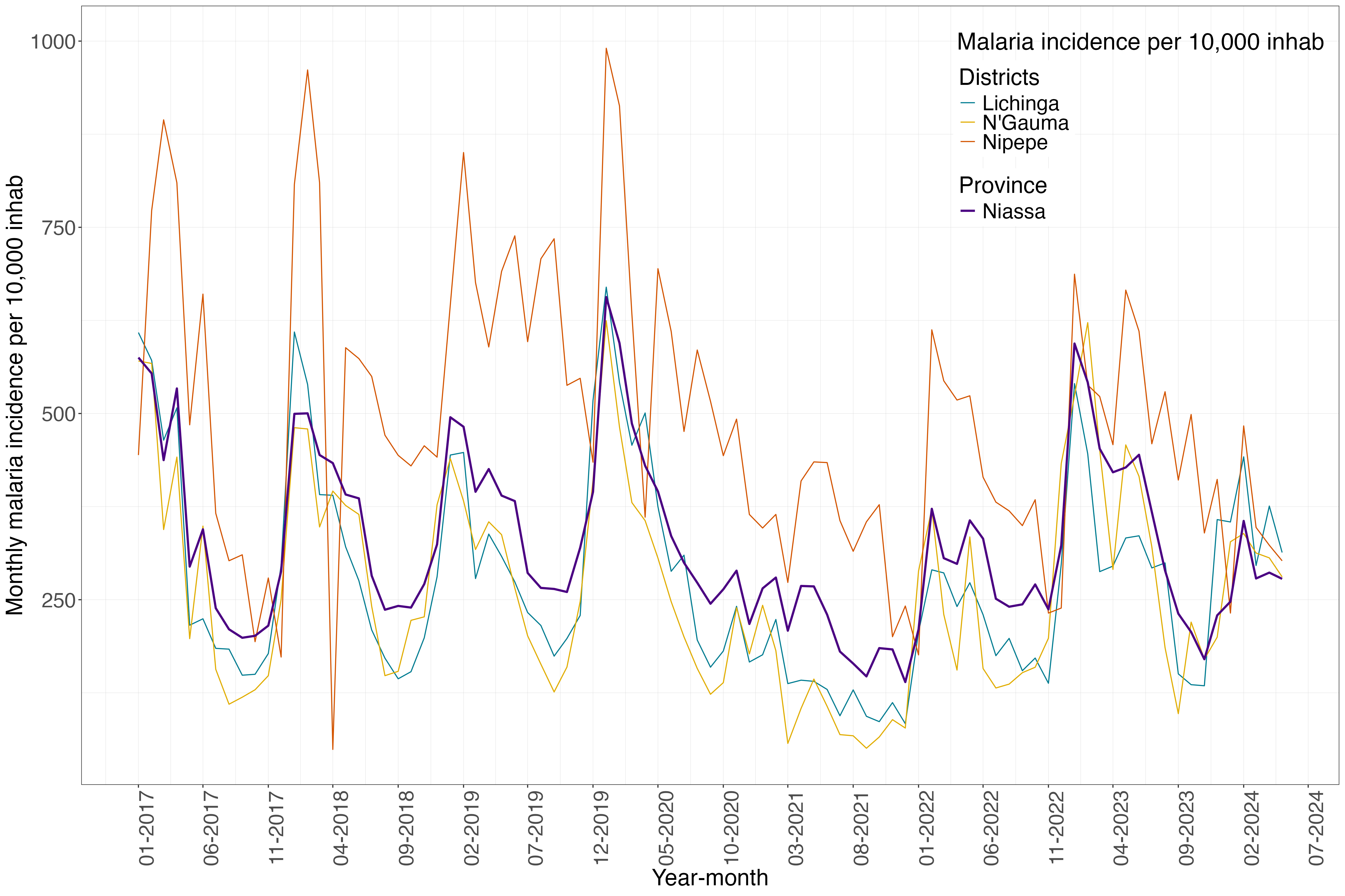
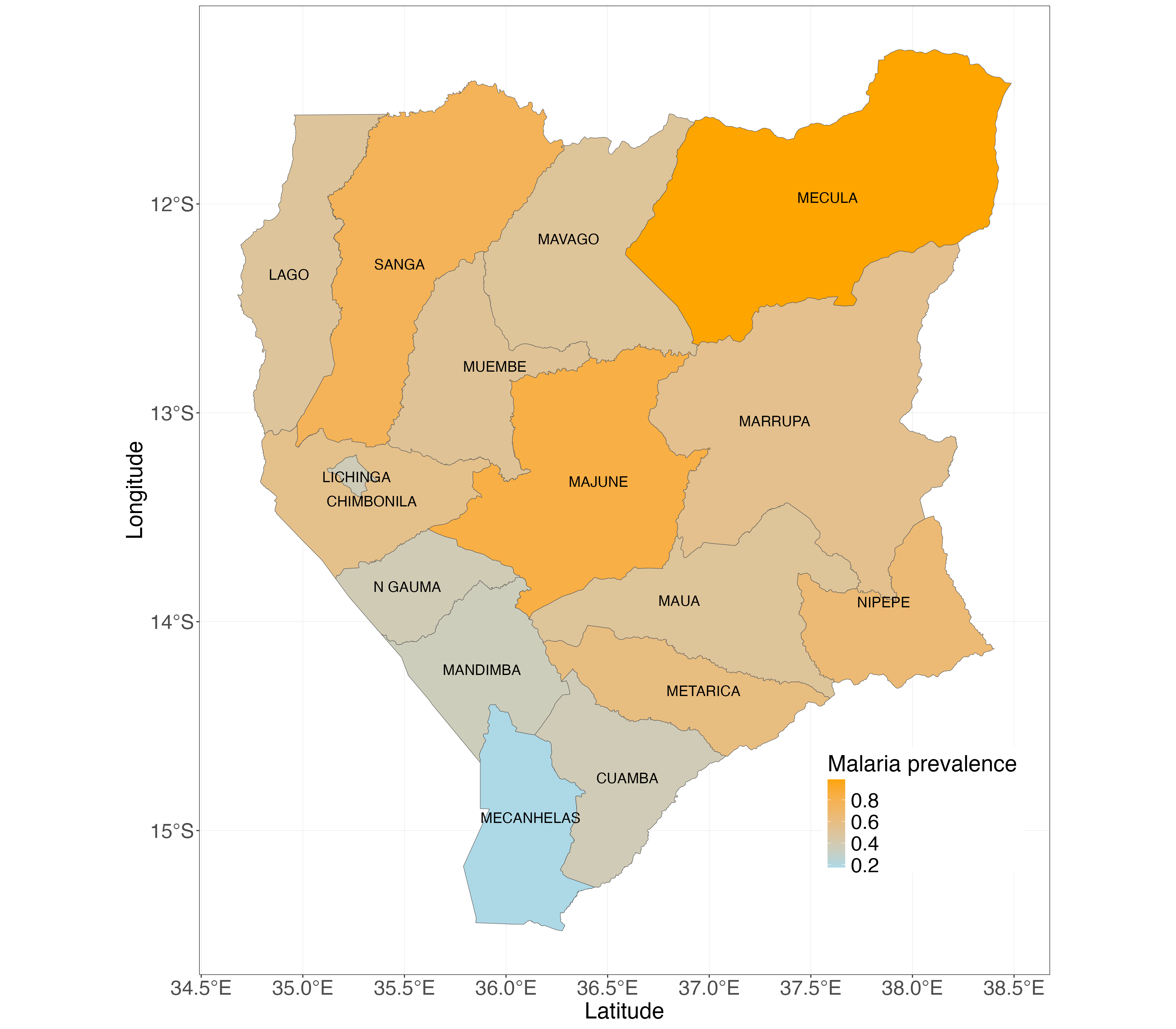
Figure 1: Exploratory visualization of malaria incidence trends in Niassa, Mozambique. Top panel: Monthly malaria incidence per 10,000 inhabitants from January 2017 to June 2024, shown for the whole Niassa province (total incidence) and three of its districts. Bottom panel: Average malaria prevalence across the province of Niassa in 2018.

Figure 2 illustrates the high spatio-temporal variability in the average prevalence of insufficient food consumption across Cameroon. For instance, the observed data suggest a consistent decline in prevalence over time in the Sud region, while the Est and Littoral regions exhibit more volatile and fluctuating patterns. Despite broad seasonal cycles in food insecurity across the country, the fluctuations differ notably by region. At the same point in time, some areas may experience severe deterioration while others remain relatively stable. The spatial heterogeneity is highlighted with prevalence levels ranging from below 0.1 in the Sud region to above 0.5 in Nord-Ouest region, possibly reflecting differences in exposure to conflict, market isolation, and humanitarian assistance.

To accommodate region-specific trajectories without over-smoothing critical local fluctuations, it is essential to adopt a modeling strategy that treats the food insecurity trajectories in each region as part of a spatially dependent collection of time series. This approach enable better tracking of both short-term shocks and longer-term structural differences between regions.

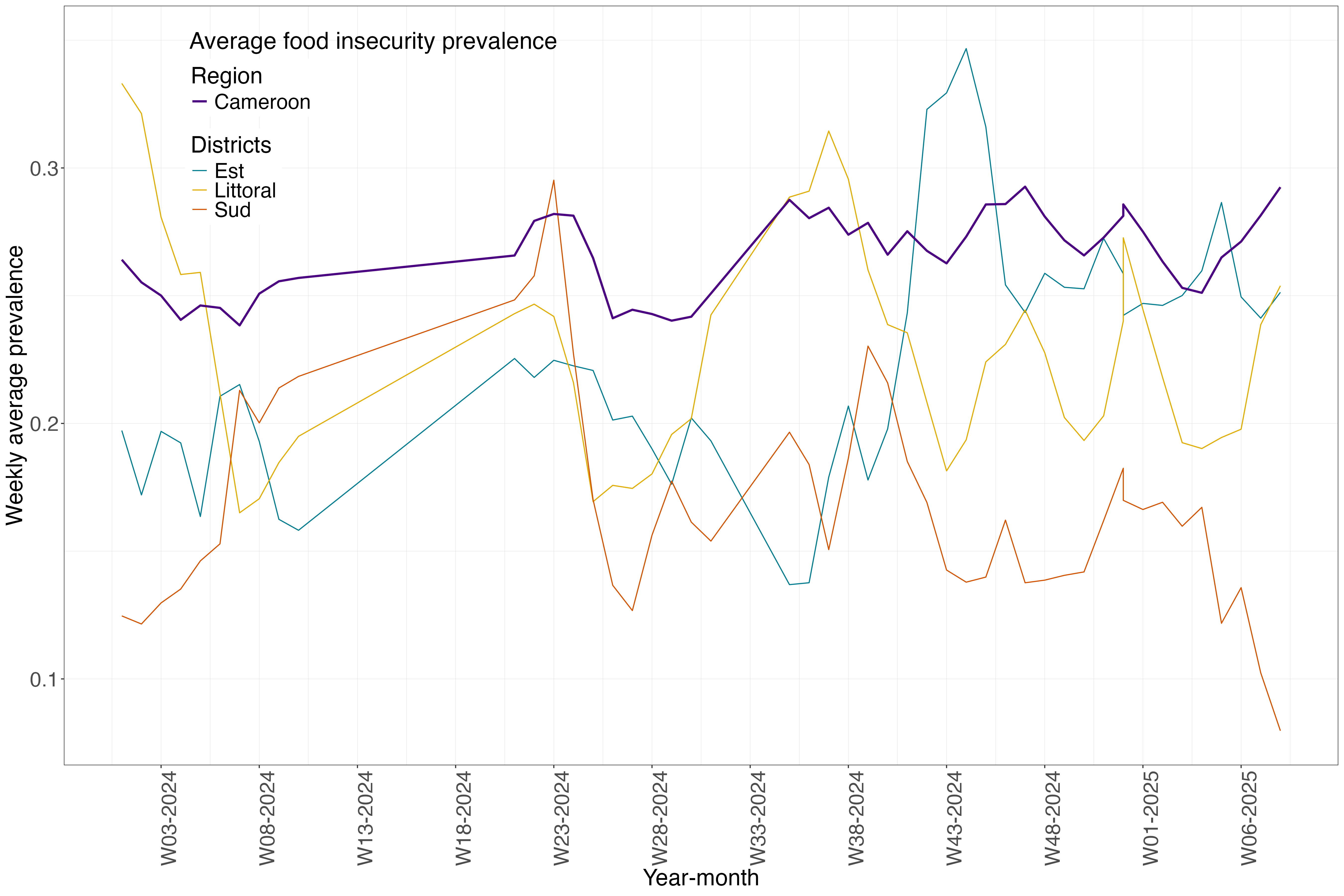
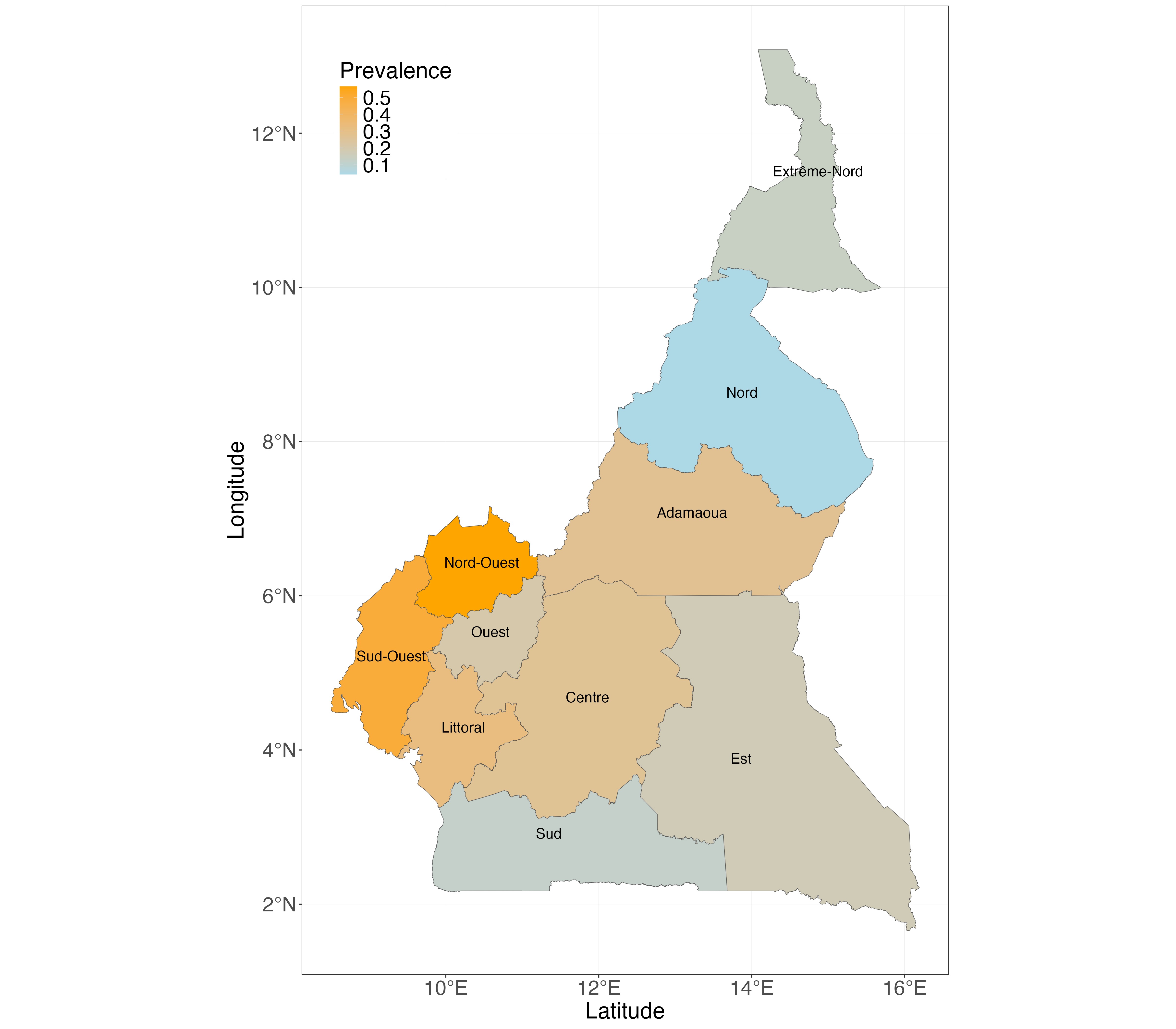
Figure 2: Exploratory visualization of insufficient food consumption across regions in Cameroon. Top panel: Average weekly prevalence of insufficient food consumption from January 2024 to February 2025, shown for the entire country and three selected regions. Bottom panel: Average prevalence of insufficient food consumption across Cameroon during the second week of January 2024.

3 Existing spatio-temporal models for areal data

Let a study area be divided into I regions, e.g., districts, counties, or municipalities, indexed by $i=1,...,I$. The temporal dimension is indexed by $t=1,...,T$, representing time points, e.g., days, weeks, or years. We denote the response variable at location $i$ and time $t$ as $Y_{it}$. The response variable’s observed data, $y_{it}$, are typically assumed to be conditionally independent random samples from a specified probability distribution, often within the exponential family. Depending on the chosen statistical model, the mean of the response variable, $\mu_{it}$, may be transformed through a link function, $g(.)$, into a scale suitable for linear modeling, represented by the linear predictor, $\eta_{it}=g(\mu_{it})$. The linear predictor is generally expressed additively as a sum of components, each capturing a distinct contribution to the variability of the outcome (López-Quılez and Munoz, 2009).

A broad class of spatio-temporal models can be represented within the following general approach towards modeling the linear predictor, $\eta_{it}$:

$$\eta_{it}=\beta_{0}+\mathbf{X_{it}}\boldsymbol{\beta}+S_{i}+D_{t}+Z_{it}+\epsilon_{it}.$$ (1)

Here, $\beta_{0}$ represents the intercept; $\mathbf{X_{it}}$ is the design matrix containing covariates that have a potential association with the outcome variable; $\boldsymbol{\beta}$ denotes the vector of coefficients associated with the covariates; $S_{i}$, $D_{t}$, and $Z_{it}$ are, respectively, spatial, temporal, and spatio-temporal model components; and $\epsilon_{it}$ corresponds to the unstructured heterogeneity term. For Gaussian linear models, $\epsilon_{it}$ represents a convolution of unstructured extra-variability and Gaussian noise; for Poisson or binomial models, where the distributional error is a direct function of the mean, and therefore not separately estimated, $\epsilon_{it}$ only captures unstructured extra-variability. It is not our intention to provide an in-depth technical description or overview of existing models belonging to this class. The summary we are about to present draws primarily from existing reviews, including López-Quılez and Munoz (2009); Wang et al. (2024); Nazia et al. (2022) and MacNab (2022). Readers interested in detailed model formulations are encouraged to consult these references directly.

Several approaches model spatial and temporal effects additively, i.e., the linear predictor in equation (1) does not contain $Z_{it}$. For the spatial component, $S_{i}$, a variety of priors have been proposed: e.g., a CAR prior, often combined with a Gaussian prior for spatial unstructured extra-variability, yielding the BYM approach (Besag et al., 1991); the Leroux prior (Leroux et al., 2000), an adaptive CAR prior (MacNab, 2023); or a spatial autoregressive (SAR; Anselin (1992)) prior. MacNab (2022) offers a comprehensive review. Similarly, temporal components, $D_{t}$, are typically modeled using structures such as AR processes, random walks, or temporally CAR priors. For example, Napier et al. (2016) specify a CAR model for spatial effects at each time point and a common temporal trend modeled through a first-order random walk.

Other models explicitly account for space-time interactions. Knorr-Held (2000) provides a comprehensive starting point, by starting from an additive model, where both $S_{i}$ and $D_{t}$ each consist of structured terms, CAR random effects and random walks, respectively, along unstructured Gaussian random effects. Additionally, $Z_{it}$, an explicit spatio-temporal component, is parameterized according to four possible specifications based on which spatial and temporal mechanisms interact, i.e., via structured or unstructured terms. Sahu and Böhning (2022) provide a more parsimonious version of the Knorr-Held model, by parameterizing $S_{i}$ and $D_{t}$ only through structured random effects, while $Z_{it}$ is modeled via random walks, AR, or CAR processes. MacNab (2011, 2007) models $S_{i}$ via CAR models, $D_{t}$ through a fixed spline for non-linear risk trends, and $Z_{it}$ through spatially varying splines. One may instead model the spatio-temporal component using tensor products splines, as discussed in Ugarte et al. (2017) and Feng (2022).

Alternative modeling approaches include only the spatio-temporal interactions, $Z_{it}$, in the linear predictor, excluding $S_{i}$ and $D_{t}$. For instance, Rushworth et al. (2014) model the interaction term using a multivariate first- or second-order autoregressive process with a spatially autocorrelated precision matrix. Rushworth et al. (2017) and Gao and Bradley (2019) propose adaptive CAR structures for the spatio-temporal interaction term. Here, the spatial adjacency matrix is treated as unknown and is estimated from the data. In contrast, MacNab (2018), Corpas-Burgos and Martinez-Beneito (2020), and Reich and Hodges (2008) propose a spatial structure that can be specified using a fixed adjacency matrix, with spatially varying scale or precision parameters introduced to modulate local dependence and interaction effects. MacNab (2023) provides a comprehensive discussion of these models and their implementation in spatio-temporal settings, while also providing further generalizations.

4 A spatially correlated Gaussian-process time-series model for areal data

Classical ST models exploit correlation by borrowing strength across neighboring areas and time points, which can improve stability and precision. However, these models frequently impose a common spatio-temporal structure across time and space, limiting their ability to capture localized deviations or region-specific dynamics. We, therefore, propose a more flexible modeling framework that retains the benefits of information borrowing across space and time but introduces greater adaptability to how temporal changes are modeled within each location. This enables a more nuanced understanding of local temporal patterns and supports more reliable long-term inference.

Building upon the notation introduced in Section 3, we now present a parameter-driven spatio-temporal modeling framework, with the corresponding linear predictor given by,

$$\eta_{it}=\mathbf{X_{i}}\boldsymbol{\beta_{i}}+Z_{it}+\epsilon_{it},$$ (2)

where $\mathbf{X_{i}}$ denotes the design matrix containing the covariates of interest, $\boldsymbol{\beta_{i}}$ the region-specific regression coefficients, and $\boldsymbol{Z_{i}}=(Z_{i1},\ldots,Z_{iT})$ the temporal Gaussian process at region $i$, assumed stationary and isotropic. This process has a zero-mean and a covariance function of the form,

$$\gamma_{i}(h)=cov(Z_{it},Z_{it^{\prime}})=\sigma_{i}^{2}\rho_{i}(h),$$ (3)

where $h$ denotes the Euclidean distance between time points $t$ and $t^{\prime}$, and $\rho_{i}(h)$ is a Matérn correlation function (Matérn, 2013) given by

$$\rho(h)=\left(2^{(\kappa-1)}\right)\Gamma(\kappa)^{-1}\left(\frac{h}{\phi_{i}}\right)^{\kappa}\mathrm{K}_{\kappa}\left(\frac{h}{\phi_{i}}\right),h>0.$$ (4)

Here, $\kappa$ controls the smoothness of the process and it is assumed fixed; $\phi_{i}$ is a temporal scale parameter that determines the range of the temporal correlation; $\Gamma(\cdot)$ is the gamma function; and $\mathrm{K}_{\kappa}(\cdot)$ is the modified Bessel function of the second kind.

To introduce spatial dependence, we specify spatial Bayesian priors on key parameters present in equations 3 and 4: we assume that (i) the log-transformed temporal variance parameters $(\log(\sigma^{2}_{1}),$ $\ldots,$ $\log(\sigma^{2}_{I}))$ follow a CAR prior using a Queen contiguity matrix to define spatial adjacency; and that (ii) the log-range parameter $\log(\phi_{i})$ follows a Gaussian distribution conditionally on $\log(\sigma^{2}_{i})$, i.e. $\log(\phi_{i})|\log(\sigma^{2}_{i})\sim\mathcal{N}(\mu(\log(\sigma^{2}_{i})),\chi^{2})$, with mean $\mu(\log(\sigma^{2}_{i}))$ and variance $\chi^{2}$ derived from the empirical relationship between $\log(\phi_{i})$ and $\log(\sigma^{2}_{i})$ estimated from district-specific models via maximum likelihood. This conditional dependence of $\log(\phi_{i})$ on $\log(\sigma^{2}_{i})$ induces spatial structure in the temporal correlation range.

This approach reflects the idea that each region follows its own temporal process, but the parameters governing these time series, more particularly their variability and scale, are not independent across space. By allowing the temporal variance and correlation structure to vary spatially, we account for the fact that regions may differ in how they evolve over time, yet nearby regions are likely to exhibit related latent dynamics due to shared unmeasured factors. Imposing spatial structure on the residual variability allows us to model this unexplained correlation without requiring extensive contextual knowledge about covariate-level spatial dependencies or interactions. In this way, spatial dependence is captured through the evolution of the temporal dynamics themselves, leading to a more flexible and interpretable framework.

When we assume that $y_{it}$ follows a Gaussian distribution, the term $\epsilon_{it}$ is a Gaussian noise term, i.e., $\epsilon_{i}\sim\mathcal{N}(0,\tau_{i}^{2})$, representing measurement error and, possibly, small-scale variability not captured by the structured components of the model. In this model, each area $i$ has its associated parameters $\theta_{i}=(\boldsymbol{\beta_{i}},\sigma^{2}_{i},\phi_{i},\nu^{2}_{i})$, where $\nu^{2}_{i}=\tau^{2}_{i}/\sigma^{2}_{i}$ is a signal-to-noise ratio.

For the remaining parameters, we specify the following priors: we assign to the log signal-to-noise ratio parameter an informative univariate Gaussian prior, $\log(\nu^{2}_{i})\sim\mathcal{N}(\mu_{\nu},\sigma^{2}_{\nu})$; for the regression coefficients, we use a non-informative multivariate Gaussian prior, $\log(\boldsymbol{\beta_{i}})\sim\mathcal{N}_{p+1}(0,10^{5}I_{p+1})$, where $p$ denotes the number of covariates and $I_{p+1}$ denotes the identity matrix of dimension $p+1$. A detailed description of the prior and hyperprior distributions, and their justification, is provided in the Supplementary Material (Section 1.1).

Note that when no spatial correlation is assumed in the variance and range parameters of the Gaussian processes, the model of equation (2) reduces to a model with independent time series for each region, which will be referred to as the independent GP time-series model. This approach prevents regions from borrowing strength to improve precision and stabilize estimates. We use the region-specific estimates of $\log(\sigma_{i}^{2})$, $\log(\phi_{i})$ and $\log(\nu_{i}^{2})$ from these models to calibrate the mean components of the prior distributions of $\log(\phi_{i})$ and $\log(\nu_{i}^{2})$ in our new spatially correlated Gaussian-process model.

4.1 Model estimation and prediction

Since the parameters of interest, $\boldsymbol{\theta}=(\theta_{1},\ldots,\theta_{I})$, are inferred within a Bayesian framework, they are treated as unobserved random variables. Inference is based on the posterior distribution, $p(\boldsymbol{\theta}\mid\boldsymbol{y})$, which represents the distribution of the parameters given the observed data, $\boldsymbol{y}$, obtained via Bayes’ Theorem. As is typical in hierarchical models, the posterior has no closed-form expression; we therefore rely on approximate inference via posterior sampling, specifically using Markov chain Monte Carlo (MCMC) methods.

Given the hierarchical structure of the model, different sampling strategies are employed depending on the form of the full conditional distributions. The MCMC algorithm proceeds iteratively, with each iteration consisting of the following steps.

Step 1 – Sampling the variance parameters: At the beginning of each MCMC iteration, the GPs’ variance parameters $(\log(\sigma^{2}_{1}),\ldots,\log(\sigma^{2}_{I}))$ are updated using the Metropolis–adjusted Langevin Algorithm (MALA) (Rossky et al. (1978); Roberts and Tweedie (1996)).

Step 2 – Sampling remaining region-specific parameters: For each region $i=1,\ldots,I$, the remaining parameters are updated conditional on the current values at a given iteration, $k$, in the following order: (i) the log-range parameter, $\log(\phi_{i})$, sampled using MALA; (ii) the log signal-to-noise ratio, $\log(\nu^{2}_{i})$, sampled via an independent Metropolis–Hastings (MH) step; (iii) the regression coefficients, $\log(\boldsymbol{\beta_{i}})$, sampled from their multivariate Gaussian full conditional distribution using a Gibbs sampler; and (iv) the temporal GP random effects, $Z_{i}=(Z_{i1},\cdots,Z_{iT})$, also sampled via Gibbs sampling. A detailed description of the sampling procedure, including the rationale for its selection, is provided in the Supplementary Material (Section 1.2).

The posterior predictive inference is based on the predictive distribution, which integrates over the uncertainty in the model parameters. Specifically, forecasts are obtained by drawing from the posterior predictive distribution $p(\boldsymbol{y^{\text{new}}}\mid\boldsymbol{y})=\int p(\boldsymbol{y^{\text{new}}}\mid\boldsymbol{\theta})p(\boldsymbol{\theta}\mid\boldsymbol{y})\,d\boldsymbol{\theta}$. This approach allows us to account for both parameter and observational variability. Predictive samples are generated via Gibbs sampling.

4.2 Model implementation

The proposed model is implemented in R (version 4.4.1 (2024-06-14); R Core Team (2021)) using the sampling strategies described in Section 4.1. We fit the model to both examples, using the malaria data and food insecurity data examples, with equations 5 and 6 describing their respective model structure:

$$\log\left(Y_{it}\right) =\eta_{it},$$ (5)

$$\eta_{it} =\beta_{0i}+\beta_{1i}\sin\left(\frac{2\pi t}{12}\right)+\beta_{2i}\sin\left(\frac{2\pi t}{6}\right)$$

$$+\beta_{3i}\cos\left(\frac{2\pi t}{12}\right)+\beta_{4i}\cos\left(\frac{2\pi t}{6}\right)+Z_{it}+\epsilon_{it},$$

and

$$\text{logit}(Y_{it}) =\eta_{it},$$ (6)

$$\eta_{it} =\beta_{0i}+\beta_{1i}\sin\left(\frac{2\pi t}{12}\right)+\beta_{2i}\cos\left(\frac{2\pi t}{12}\right)+Z_{it}+\epsilon_{it}.$$

In Equation 5, $Y_{it}$ denotes the monthly malaria incidence in district $i$ at month $t$, while in equation 6, $Y_{it}$ represents the average prevalence of individuals with insufficient food consumption in region i at week t . To meet the normality assumptions, we apply a log transformation to the incidence proportions in the malaria data and an empirical logit transformation to the prevalence values in the food insecurity data. These transformations help to stabilize variance, improve model predictions, and support the Gaussian assumption on the transformed scale. As explanatory variables, we include first- and second-degree Fourier terms to capture large-scale seasonal patterns. The degree was selected based on the Akaike Information Criterion (AIC) values from simpler linear models with varying Fourier terms.

For each motivating example, we ran the MCMC algorithm for 50,000 iterations, which includes a burn-in period of 10,000, while adopting a thinning interval of 10, resulting in 4,000 posterior samples for each parameter. Trace plots, autocorrelation plots, and Geweke running plots were used for visual inspection of the convergence, in addition to the Geweke diagnostic as a formal assessment. Computation was performed using the Flemish Supercomputer Center (VSC) facilities.

For each application, the data were partitioned into training and test sets. In the case of the malaria data analysis, the training set covered the period from January 2017 to September 2023, and the test set comprised data from October 2023 to June 2024. Similarly, for the food insecurity data study, the training set spanned from January 2024 to September 2024, corresponding to 37 weeks of analysis and, the test set from mid-September 2024 to mid-November 2024, containing 9 weeks. This division was designed to evaluate the model’s out-of-sample predictive performance.

4.3 Model performance evaluation

To assess the performance of our proposed model, we compared it against four alternatives, each representing a set of important variations in modeling approaches found in the literature: (1) the spatio-temporal model with space-time interaction by Knorr-Held (2000), with the so-called Type I interaction, i.e., interaction between unstructured spatial and unstructured temporal components; (2) the spatio-temporal model of Rushworth et al. (2014) of the first order; (3) the spatio-temporal model of Rushworth et al. (2014) of the second order; and (4) the independent GP time-series model. These benchmark models were selected based on their theoretical relevance and the availability of public software implementations, enabling their use across our case studies as well as in applied research more generally. Models (1)–(3) were implemented using the CARBayesST R package (Lee and Lawson, 2016). The independent GP time-series model was implemented using the PrevMap R package (Giorgi and Diggle, 2017). Note that although PrevMap has originally been developed for geostatistical modeling using spatial coordinates, it can be adapted for time series applications by treating time as a one-dimensional coordinate and pairing it with a constant vector of ones instead of spatial coordinates. Other models available in CARBayesST, such as those proposed by Napier et al. (2016) and Lee and Lawson (2016), were excluded due to their reliance on discrete outcome distributions, e.g., the Poisson or binomial distributions, which are not compatible with our modeling framework. Similarly, more recent approaches involving adaptive spatial structures (e.g., MacNab, 2023; Corpas-Burgos and Martinez-Beneito, 2020) were not considered due to the lack of commonly available implementations in R.

For models (1) to (3), we ran the MCMC algorithm for 50,000 iterations, with a burn-in period of 10,000 and a thinning interval of 10, yielding 4,000 posterior samples for each parameter. As with the spatially correlated Gaussian-process model, we assessed convergence using both graphical and formal diagnostics. The following subsection provides the detailed specifications of the four models used to benchmark our approach.

4.3.1 Model specification of benchmark models

Model (1), which applies the approach of Knorr-Held (2000), is parametrized as,

$$\eta_{it}=\beta_{0}+\sum_{j=1}^{J}\left(\beta_{ij}^{(s)}\sin\left(\frac{2\pi jt}{12}\right)+\beta_{ij}^{(c)}\cos\left(\frac{2\pi jt}{12}\right)\right)+S_{i}+D_{t}+Z_{it},$$ (7)

where $\eta_{it}$ represents the linear predictor for region $i$ and time $t$, and $\beta_{ij}^{(s)}$, $\beta_{ij}^{(c)}$ are Fourier coefficients associated with the $j^{\text{th}}$ sine and cosine terms, respectively. The Fourier expansion captures seasonal patterns, with the degree $J=2$ for the malaria data and $J=1$ for the food insecurity data. The degree was selected based on AIC values from simpler linear models with varying Fourier terms. Following Lee et al. (2018), $S_{i}$ and $D_{t}$ denote spatial and temporal random effects, respectively, each modeled with the Leroux conditional autoregressive (CAR) prior (Leroux et al., 2000). While the Leroux CAR prior is typically employed for spatial dependence, it is here also adopted to capture temporal correlation, using its common definition that is extended across the time dimension. In addition, $Z_{it}\sim\mathcal{N}(0,\omega_{1}^{2})$ denotes an independent space-time interaction term of the unstructured spatial and unstructured temporal random effects, also known as interaction type I.

Models (2) and (3), proposed by Rushworth et al. (2014), are specified as,

$$\eta_{it}=\beta_{0}+\sum_{j=1}^{J}\left(\beta_{ij}^{(s)}\sin\left(\frac{2\pi jt}{12}\right)+\beta_{ij}^{(c)}\cos\left(\frac{2\pi jt}{12}\right)\right)+Z_{it},$$ (8)

where $Z_{it}$ represents the spatio-temporal random effect, in addition to the other model components, which were specified as in Equation 7. More precisely, $\mathbf{z}_{t}=(z_{1t},\dots,z_{It})$ evolves over time via a multivariate autoregressive process of either the first (model 2) or second order (model 3), depending on the model variant. Temporal dependence is introduced through an autoregressive parameter $\rho$, while spatial correlation is incorporated via the precision matrix $\omega_{2}\mathbf{Q}(\mathbf{W},\rho)$, as defined by Leroux et al. (2000). The variance of the spatial process is governed by the parameter $\omega_{2}$. Priors for models (1)–(3) follow the default specifications provided in the CARBayesST R package (Lee et al., 2018).

The fourth benchmark model, an independent GP time-series model, assumes spatial independence and models the time series of each region separately. The linear predictor structure follows the structure presented in equations 5 and 6, but it assumes spatial independence between the region-specific temporal Gaussian processes. This model was implemented using the PrevMap R package (Giorgi and Diggle, 2017) and estimated via maximum likelihood for computational efficiency.

4.3.2 Comparison metrics

Model performance was assessed using both point-based and distribution-based metrics. For point-based evaluation, we computed the Root Mean Squared Error (RMSE) and Mean Absolute Error (MAE) to quantify the discrepancy between observed and predicted values. For distribution-based evaluation, we used the Continuous Ranked Probability Score (CRPS) to assess the sharpness and calibration of the posterior predictive distributions (Matheson and Winkler (1976); Gneiting and Ranjan (2011)). Additionally, we calculated the Empirical Coverage Probability (ECP) by evaluating the proportion of observed values that lie within the credible intervals produced by each model, to assess the accuracy in quantifying uncertainty. All metrics were computed for both the training and test sets to ensure consistency and fairness in model comparison.

Special attention was given to the CRPS, as it evaluates the entire predictive distribution, unlike point-based metrics such as RMSE or MAE, which compare only the predicted mean or median to the observed value. In general, CRPS rewards predictions that are both accurate and well-calibrated. Additionally, because CRPS can be computed for each observation, it enables straightforward comparisons at both global and local levels. Importantly, lower CRPS values indicate better predictive performance, as they reflect distributions that are both close to the observed values and appropriately uncertain.

5 Results

Key results are presented in the main body of the paper, with additional findings available in the Supplementary Material (Section 2). Given the large volume of results, the reader is encouraged to explore them interactively via our Shiny application: https://kj8o9q-alejandro-rozo0posada.shinyapps.io/tool_spatcorrgp_arealdata/. This tool enables an in-depth examination of both motivating examples. Users can explore the predictive performance of the proposed model, compare it against benchmark models, and assess parameter convergence diagnostics.

5.1 Malaria incidence in Niassa, Mozambique

Overall, the diagnostics indicate good convergence for most parameters, particularly the fixed effects and log signal-to-noise ratio $\log(\nu^{2})$. The log-range parameters $\log(\phi)$ and GPs’ variance parameters $\log(\sigma^{2})$ exhibited slower mixing and higher autocorrelation. Full convergence diagnostics for the parameters related to the districts Lichinga, Majune, Mecanhelas, and Sanga are available in the Supplementary Material (Section 2.1), and for all districts in the Shiny interactive tool. Additionally, the acceptance rates of the samplers for $\log(\phi)$ and $\log(\sigma^{2})$ are on average 57.02%, as expected when using MALA. For the parameters of the log signal-to-noise ratio $\log(\nu^{2})$, this rate is on average 20.45%.

Figure 3 shows the observed and estimated monthly malaria incidence in four districts of the province of Niassa. During the training period, the proposed spatio-temporal model exhibits an accurate fit, with narrow 95% credible intervals that closely follow the observed trends. This is consistently observed among all districts. For the test period, the model effectively captures the overall trend of the incidence as the observed trend generally lies within the 95% credible interval bands of the forecast incidence trends, but its performance is, as expected, not as excellent as for the training data. For instance, mean incidence forecasts in districts such as Majune and Mecanhelas tend to be overestimated, while in other districts, like Lichinga, it is underestimated. These differences reflect the inherent uncertainty in out-of-sample forecasting. Importantly, 95% prediction intervals mostly contain the true trend, in its totality, or at least to a large extent.

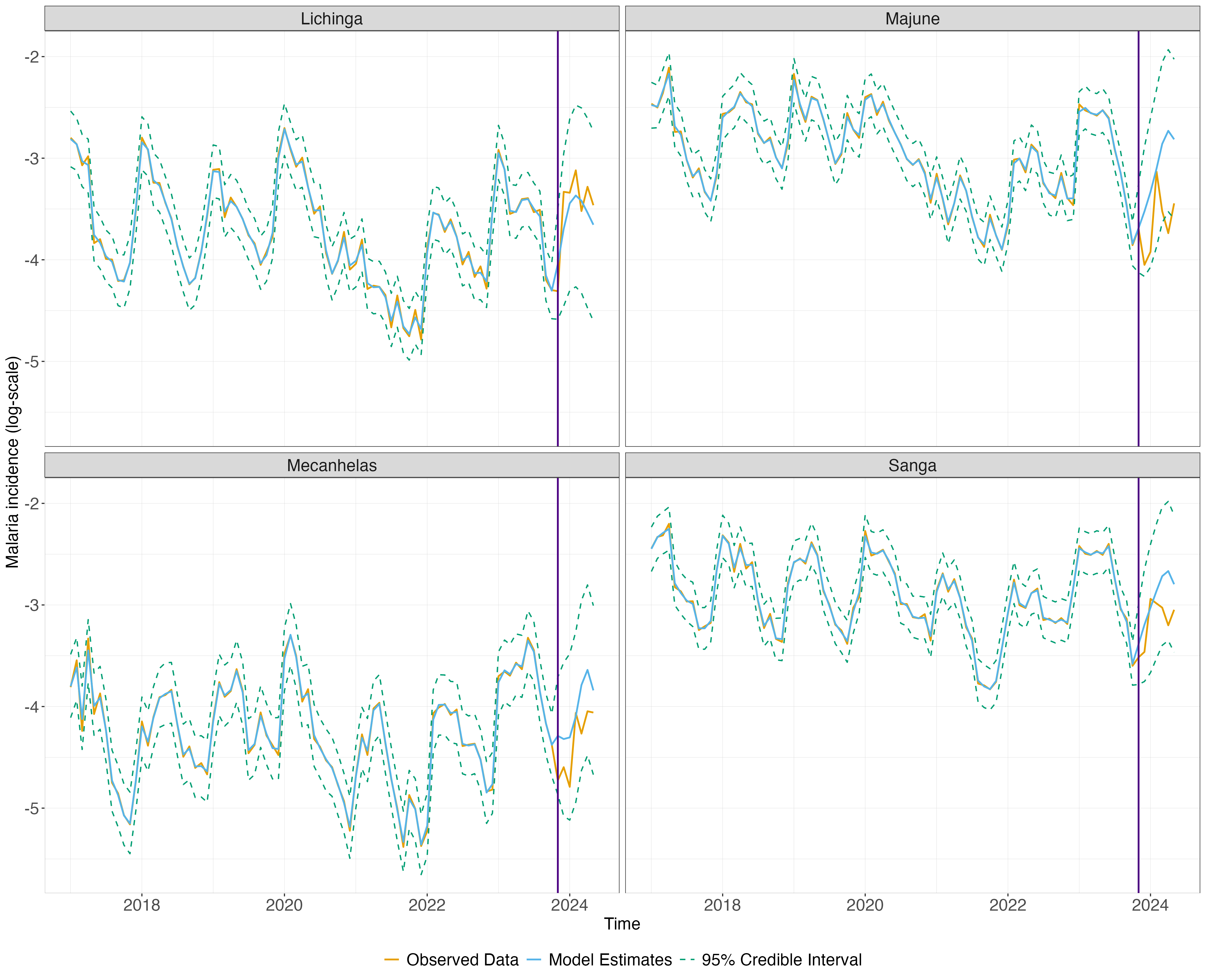
Figure 3: Model-based incidence estimates obtained from the spatially correlated Gaussian-process time-series model for the monthly malaria incidence in four districts of the Niassa province: Lichinga, Majune, Mecanhelas, and Sanga. The results are presented on the log scale and include both point estimates and the associated 95% credible intervals. The vertical purple line indicates the division between the training set (before) and test set (after).

The median CRPS results on the training and test sets demonstrate that the proposed model outperforms the competing approaches, achieving the lowest median CRPS across most districts in both sets (Figure 4). In the test set, the performance gap narrows, but the proposed model remains competitive, ranking among the best-performing models, and in many cases, outperforming all others. Notably, in many districts, the median CRPS values of the independent and spatially correlated GP models are similar. It is worth noting that these CRPS-based findings are consistent with the results obtained using pointwise performance metrics such as the RMSE and the MAE, which are presented in the Shiny interactive tool and in the Supplementary Material (Section 2.2).

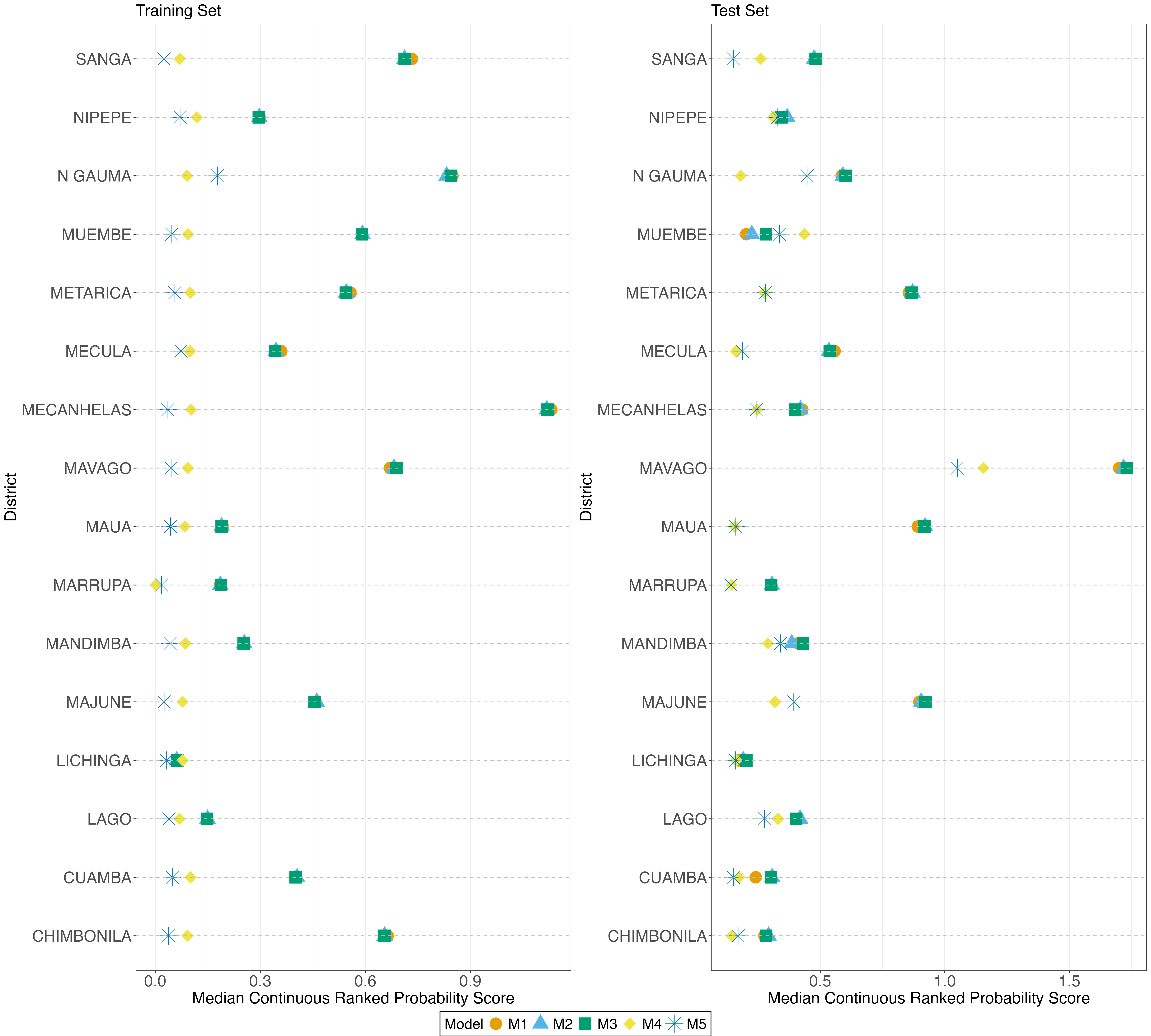
Figure 4: Comparison of model performance on the training set and test set for Malaria incidence in Niassa, Mozambique, using the Continuous Ranked Probability Score (CRPS). M1: Knorr-Held (2000), M2: first-order Rushworth et al. (2014), M3: second-order Rushworth et al. (2014), M4:independent Gaussian-process, M5: spatially correlated Gaussian-process.

Figure 5 displays the model comparison at the district level. By leveraging the fact that CRPS provides a score at each time point, we can assess the temporal variation in predictive performance. The boxplots for the training set are based on 82 time points, while those for the test set are based on 7 time points. Comparing models, we observe that the spatio-temporal approaches of Knorr-Held (2000), and the first- and second-order models of Rushworth et al. (2014) exhibit significantly greater variability in predictive performance compared to the independent and spatially correlated GP models in both training and test sets. This pattern is consistent across all districts. Moreover, when comparing the GP models, our spatially correlated version often demonstrates reduced variability in CRPS, indicating more stable predictive performance over time. These results position our proposed model in this data example, on average, as the better-calibrated and more accurate one. Additional district-level boxplots can be consulted in the Shiny interactive tool and in Section 2.2 of the Supplementary Material.

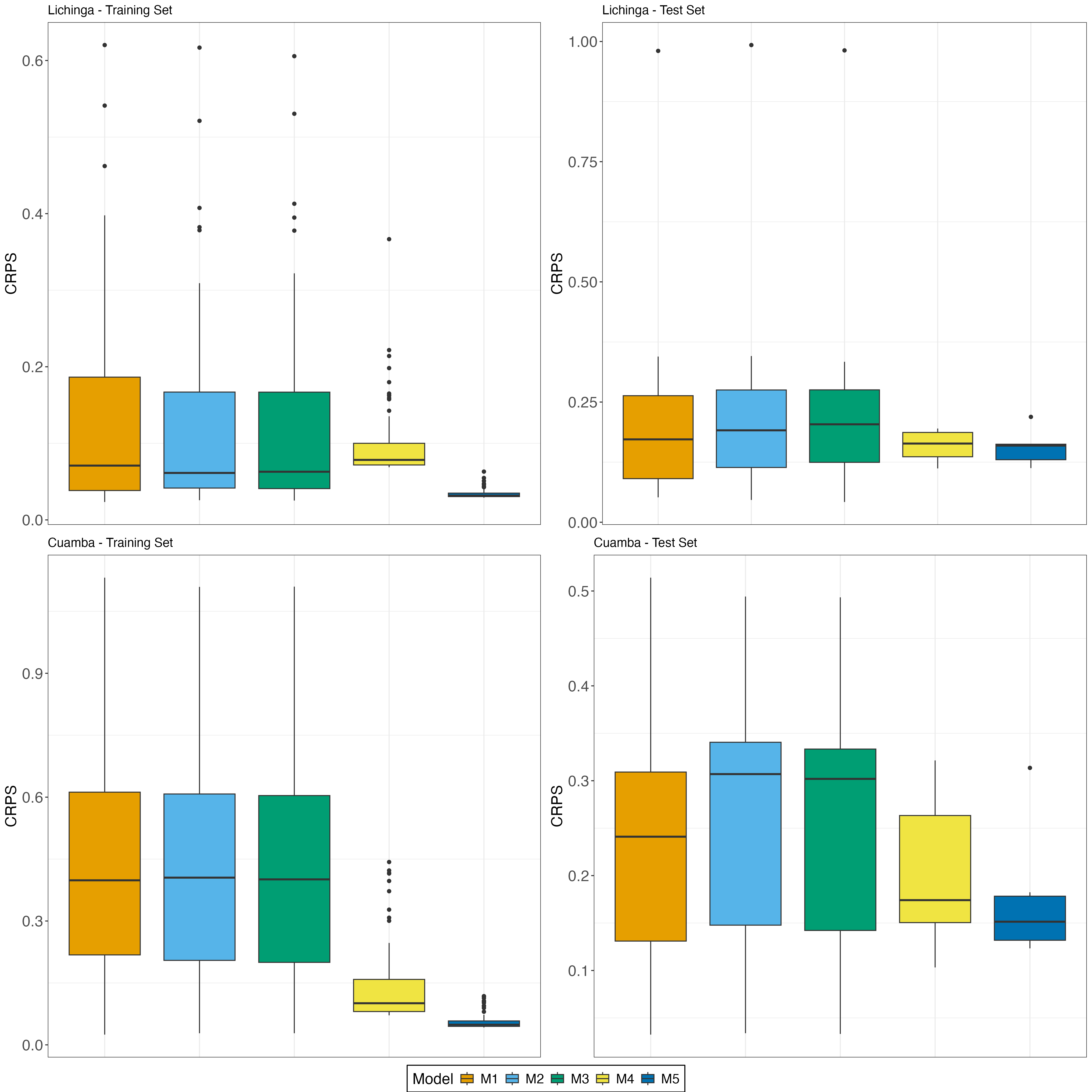
Figure 5: District-level distribution of the Continuous Ranked Probability Score (CRPS) on the training set (left panels) and test set (right panels) for malaria incidence in the districts of Cuamba (top panels) and Majune (bottom panels) in Niassa, Mozambique. M1: Knorr-Held (2000), M2: first-order Rushworth et al. (2014), M3: second-order Rushworth et al. (2014), M4: independent Gaussian-process, M5: spatially correlated Gaussian-process.

Table 1 presents the average ECP for the five different models (M1 to M5) evaluated on both the training and test sets across multiple districts. We observe that ECP values in the test set exhibit greater variability and are generally lower for several districts and models compared to the training set, highlighting a decrease in coverage when models are applied to unobserved data. Overall, the proposed model (M5) performs well across both training and test sets, consistently showing higher empirical coverage compared to other models. This suggests that M5 provides more a reliable uncertainty quantification and a better generalization to new data.

Table 1: Comparison of model performance on the training set and test set for Malaria incidence in Niassa, Mozambique, using the Empirical Coverage Probability (ECP), averaged by district. M1: Knorr-Held (2000), M2: first-order Rushworth et al. (2014), M3: second-order Rushworth et al. (2014), M4: independent Gaussian-process, M5: spatially correlated Gaussian-process.

	Training set					Test set
District	M1	M2	M3	M4	M5	M1	M2	M3	M4	M5
Lichinga	0.70	0.73	0.72	0.79	1.00	1.00	1.00	1.00	0.86	1.00
Cuamba	0.57	0.59	0.57	0.60	1.00	1.00	1.00	1.00	0.57	1.00
Lago	0.76	0.79	0.79	0.65	1.00	0.86	0.86	1.00	0.00	1.00
Chimbonila	0.51	0.51	0.51	0.74	1.00	0.86	0.86	0.86	0.86	1.00
Majune	0.65	0.71	0.71	0.76	1.00	0.29	0.29	0.29	0.43	0.86
Mandimba	0.61	0.63	0.63	0.79	1.00	0.71	0.71	0.71	0.43	0.86
Marrupa	0.62	0.68	0.67	1.00	1.00	1.00	1.00	1.00	1.00	1.00
Maua	0.66	0.68	0.68	0.76	1.00	1.00	1.00	1.00	0.86	1.00
Mavago	0.54	0.61	0.61	0.82	1.00	0.00	0.00	0.00	0.00	0.29
Mecanhelas	0.55	0.59	0.60	0.57	1.00	0.71	0.71	0.71	0.29	1.00
Mecula	0.61	0.63	0.62	0.76	0.91	0.71	0.71	0.71	0.71	1.00
Metarica	0.55	0.59	0.59	0.73	1.00	0.43	0.29	0.29	0.29	1.00
Muembe	0.50	0.54	0.56	0.85	0.95	0.14	0.14	0.29	0.57	1.00
N’Gauma	0.51	0.56	0.57	0.73	0.56	0.86	0.86	0.86	0.71	0.29
Nipepe	0.55	0.59	0.60	0.56	0.99	0.86	0.86	1.00	0.43	1.00
Sanga	0.68	0.71	0.71	0.59	1.00	0.86	1.00	0.86	0.14	1.00

5.2 Food insecurity in Cameroon

The convergence results for the food insecurity application closely mirror those of the malaria incidence in Niassa example, showing similar patterns of stability and slower mixing for the log-range parameters $\log(\phi)$ and GPs’ variance parameters $\log(\sigma^{2})$. Furthermore, the acceptance rates of the samplers for $\log(\phi)$ and $\log(\sigma^{2})$ are on average 56.75%, again as expected when using MALA. For the parameters of the log signal-to-noise ratio $\log(\nu^{2})$, this rate is on average 27.01%. Full convergence diagnostics for all parameters related to the regions Adamaoua, Nord, Nord-Ouest and Sud are available the Supplementary Material (Section 2.3), and for all regions in the country in the Shiny interactive tool.

Figure 6 displays the observed and predicted weekly prevalence of insufficient food consumption across four regions in Cameroon. Similar to the malaria data example, the proposed model fits closely to the training data and captures observed trends well during the test period, as 95% credible intervals consistently encompass them. For the test period, the model captures the observed trend, but performance is not as accurate as for the training set, although 95% prediction intervals again mostly capture the true trend.

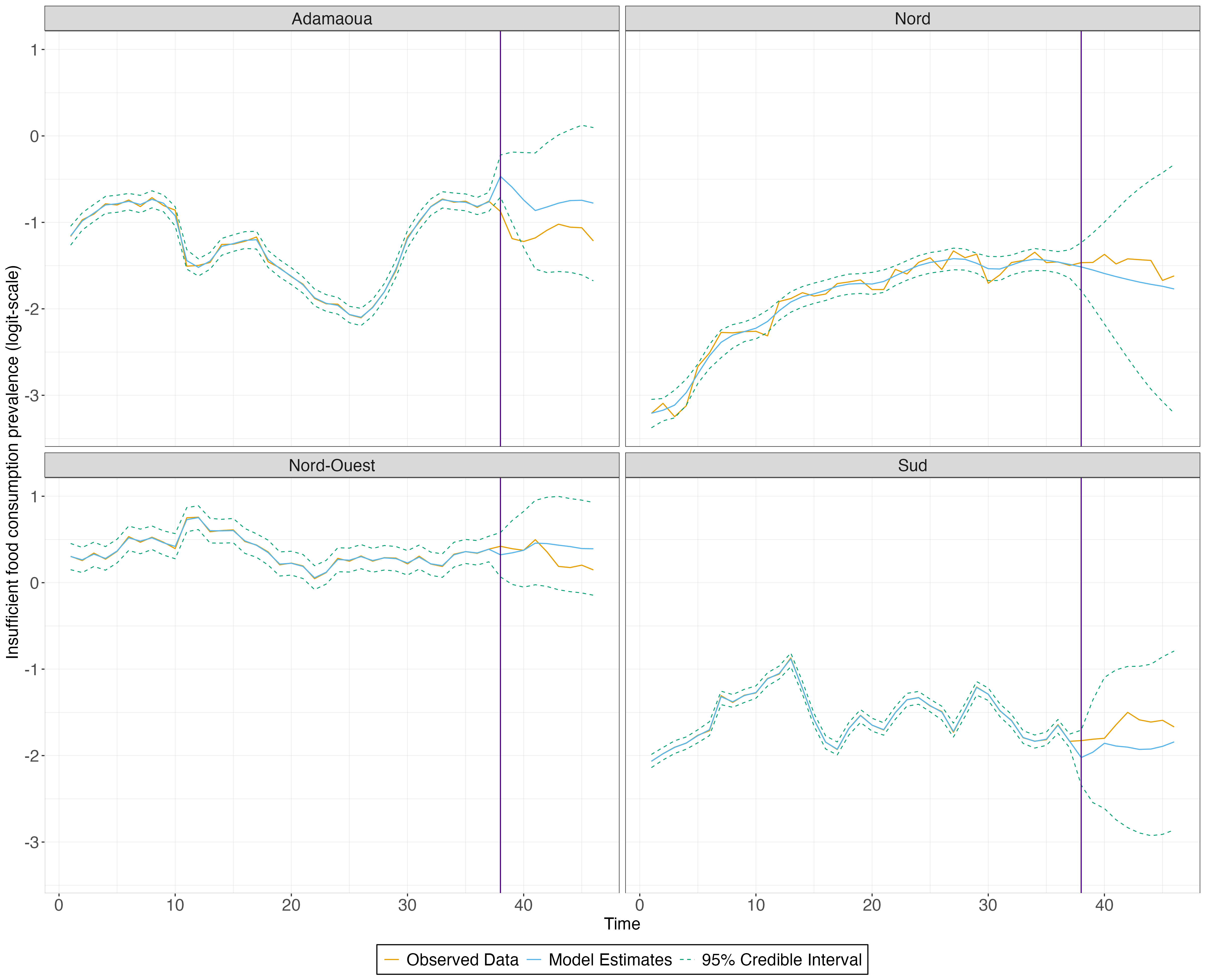
Figure 6: Model-based prevalence estimates obtained from the spatially correlated Gaussian-process time-series model for the weekly average prevalence of insufficient food consumption in four regions of Cameroon: Adamaoua, Nord, Nord-Ouest, and Sud. The results are presented on the logit scale and include both point estimates and the associated credible intervals. The vertical purple line indicates the division between the training set (before) and test set (after).

In the training set, the independent and spatially correlated GP models frequently achieve the lowest or near-lowest CRPS across most regions (Figure 7), indicating strong predictive performance. The test set shows a similar trend in many regions, where these GP models often outperform the other three spatio-temporal models. However, in Center and Extreme-Nord, the CRPS of M5 is higher than the best-performing models, suggesting weaker performance there. Overall, the proposed model demonstrates consistently strong results in both sets, with only a few regions as exceptions. These results closely align with those obtained using the RMSE and the MAE, which are presented in the Supplementary Material (Section 3.4) and in the Shiny interactive tool.

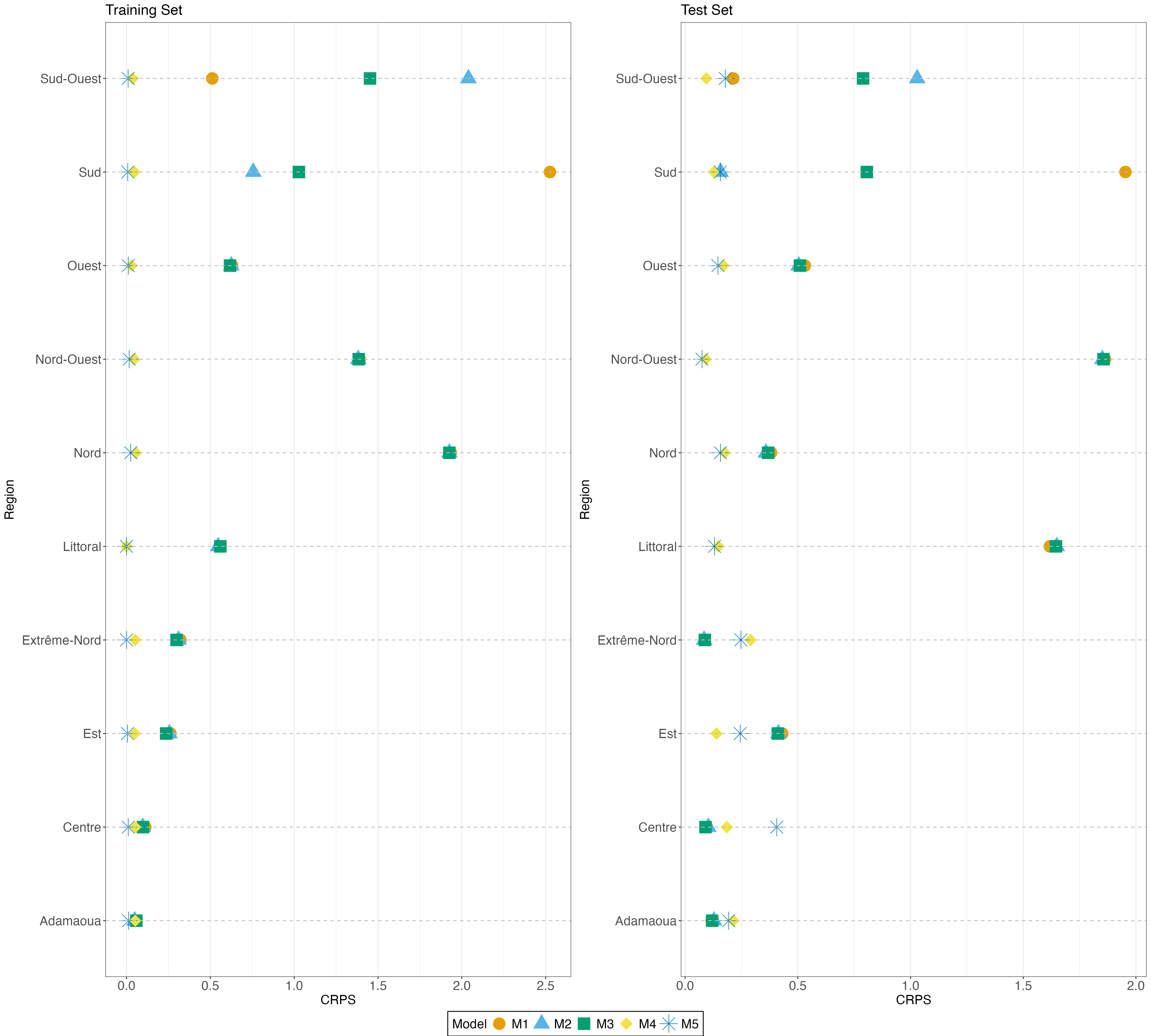
Figure 7: Comparison of model performance on the training set and test set for food insecurity in Cameroon, using the Continuous Ranked Probability Score (CRPS). M1: Knorr-Held (2000), M2: first-order Rushworth et al. (2014), M3: second-order Rushworth et al. (2014), M4: independent Gaussian-process, M5: spatially correlated Gaussian-process.

At the regional level, Figure 8 focuses on the regions Nord and Littoral. The spatio-temporal approaches of Knorr-Held (2000) and Rushworth et al. (2014) (first and second orders) show greater variability in predictive performance compared to the independent and spatially correlated GP models, for most areas. These results suggest that the GP models produce more stable predictions compared to other models. When comparing the two Gaussian-process models (M4 and M5), the spatially correlated approach exhibits more variability than the independent case. However, in some cases the differences between the two are very small. Section 2.4 of the Supplementary Material presents the region-level distribution of CRPS for a set of the remaining areas. The results for all the regions can be consulted in the Shiny interactive tool.

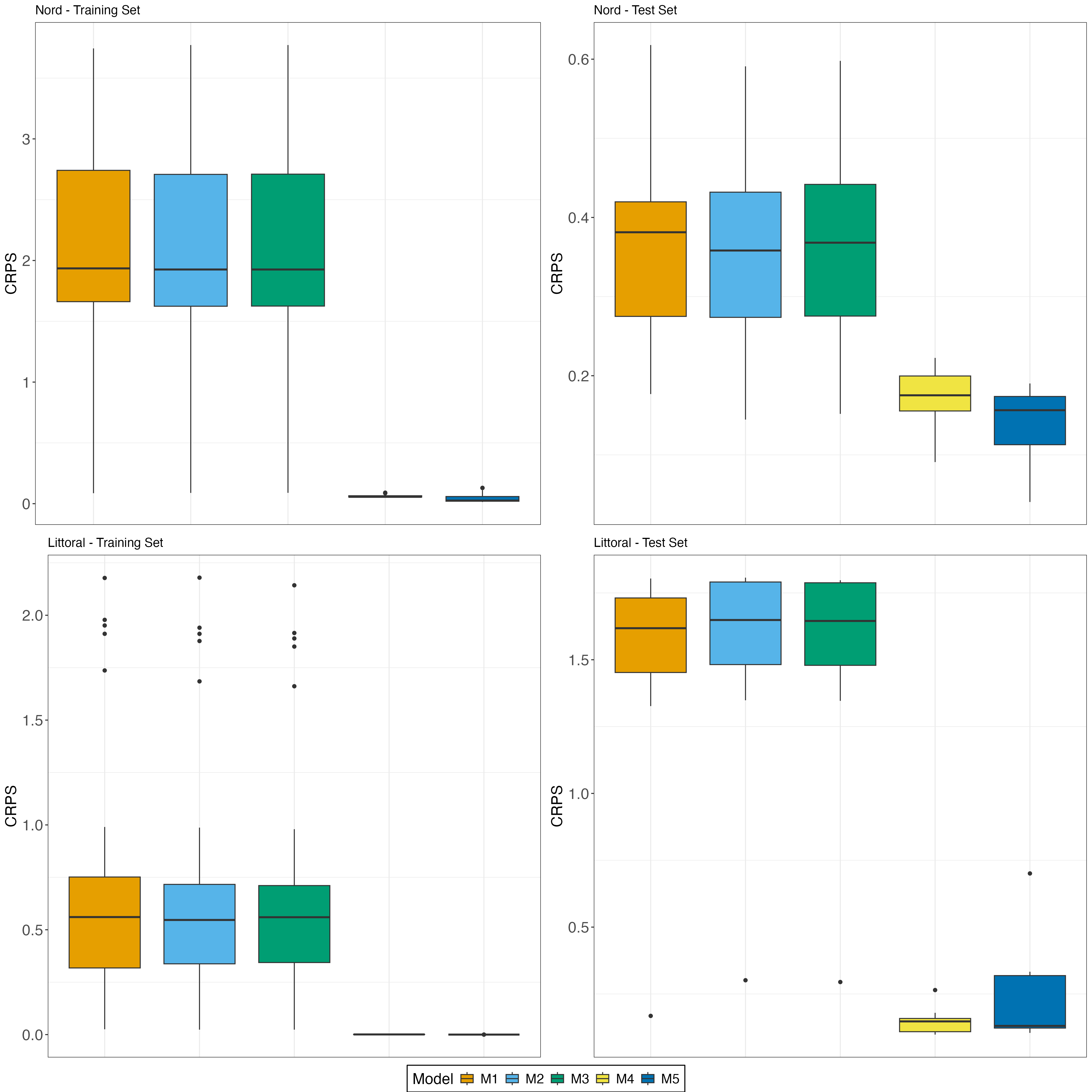
Figure 8: Region-level distribution of the Continuous Ranked Probability Score (CRPS) on the training set (left panels) and test set (right panels) for food insecurity in the region of Littoral (top panels) and Ouest (bottom panels) in Cameroon. M1: Knorr-Held (2000), M2: first-order Rushworth et al. (2014), M3: second-order Rushworth et al. (2014), M4: independent Gaussian-process, M5: spatially correlated Gaussian-process.

In Table 2, we observe the average ECP for the five models across regions in Cameroon, for both training and test sets. Similar to the malaria data analysis, ECP values for test data are more variable and generally lower than for training data, reflecting reduced coverage on new data. Despite this, GP models consistently perform well, providing reliable uncertainty estimates and better generalization across regions than other spatio-temporal models.

Table 2: Comparison of model performance on the training set and test set for Food insecurity in Cameroon, using the Empirical Coverage Probability (ECP), averaged by region. M1: Knorr-Held (2000), M2: first-order Rushworth et al. (2014), M3: second-order Rushworth et al. (2014), M4: independent Gaussian-process, M5: spatially correlated Gaussian-process.

	Training set					Test set
Region	M1	M2	M3	M4	M5	M1	M2	M3	M4	M5
Adamaoua	0.73	0.70	0.68	0.95	1.00	0.00	0.11	0.11	0.78	0.78
Centre	0.54	0.68	0.65	1.00	1.00	0.00	0.44	0.00	0.56	0.89
Est	0.51	0.51	0.51	1.00	1.00	0.00	0.78	0.56	1.00	1.00
Extreme-Nord	0.62	0.65	0.70	1.00	1.00	0.11	1.00	1.00	0.78	1.00
Littoral	0.59	0.70	0.68	1.00	1.00	0.00	1.00	0.44	0.89	0.89
Nord	0.70	0.76	0.73	0.84	0.92	1.00	0.00	0.33	1.00	1.00
Nord-Ouest	0.81	0.89	0.95	0.84	1.00	1.00	0.00	0.89	1.00	1.00
Ouest	0.89	0.92	0.92	1.00	1.00	1.00	0.00	0.11	1.00	1.00
Sud	0.62	0.65	0.68	1.00	1.00	1.00	0.00	0.00	1.00	1.00
Sud-Ouest	0.95	0.95	0.97	1.00	1.00	1.00	0.00	0.22	1.00	1.00

6 Discussion

This work aimed to develop a flexible and robust modeling framework capable of capturing complex spatio-temporal dependencies in areal data. The proposed approach adopts a hierarchical structure, incorporating region-specific fixed effects alongside temporally smooth trends modeled by Gaussian processes. Temporal correlation is addressed via the GP structure, while spatial dependence is introduced through spatially linked variance parameters across regions, facilitating flexible information sharing among neighboring regions. The model was applied to two motivating case studies, i.e., malaria incidence in Niassa, Mozambique, and food insecurity prevalence in Cameroon. It demonstrated excellent in-sample performance with accurate estimates and narrow credible intervals. Out-of-sample predictions were as expected: less accurate, but still effective at capturing key temporal trends, with $95\%$ prediction intervals almost always covering observed values. These findings highlight the potential of the framework for monitoring and forecasting applications in complex spatio-temporal settings, especially where local heterogeneity plays a key role.

While our approach shares key objectives with traditional spatio-temporal models, namely, smoothing estimates and quantifying uncertainty in unobserved locations, it differs from them in its foundation. Classical models often extend spatial methods into the temporal domain using parametric structures such as AR or RW processes. In contrast, we start from a time-series perspective and generalize this toward the spatial setting, using non-parametric GPs to model time with greater flexibility and interpretability. Similar to the approach of Rushworth et al. (2014) and Lee and Lawson (2016), we incorporate spatial dependence via the variance parameters, but we go one step further by allowing region-specific temporal parameters, improving the model’s ability to smooth over time and adapt to local temporal trends. We compared the performance of our model, both in terms of in-sample estimation, and out-of-sample prediction, to a set of commonly used spatio-temporal models that are readily available through the implementation in the CARBayesST R package (Lee et al., 2018). Our method generally outperformed these methods when it came to in-sample estimation, and outperformed or competed with the other methods in out-of-sample prediction performance.

Across both motivating examples, the spatially correlated Gaussian-process model achieved consistently strong performance in terms of the CRPS, often matching or outperforming other models in both the training and test sets. In both examples, lower CRPS values are complemented by very high ECP, in many cases equal to 1, which may indicate overly wide credible intervals. However, the combination of high coverage and lower CRPS in the test sets suggests that the model effectively generalizes uncertainty without suffering from overfitting.

The proposed modeling framework is general in its structure, allowing for any suitable mean specification. In our examples, we included Fourier terms to account for large-scale seasonal effects; additional, i.e., residual, variation was captured by the GP-based random effects and the Gaussian noise term. While this approach already demonstrated strong performance, we recognize that incorporating context-relevant covariates, such as environmental drivers or mobility data, could improve explanatory power and forecasting accuracy. For the purpose of developing and testing the proposed methodology, however, we explicitly chose to keep the specification of the mean simple, such that there remained enough spatio-temporal extra-variability in the residual model component.

There are, however, a number of limitations to our proposed modeling framework. First, the current implementation is computationally intensive, with runtimes of approximately 72 and 51 hours for the malaria data and food insecurity data analyses, respectively. These durations are primarily due to high-dimensional MCMC sampling required for non-tractable posteriors. Future developments will aim to optimize the algorithm, drawing on techniques from existing efficient packages such as CARBayesST (Lee et al., 2018). Possible strategies include leveraging Rcpp (Eddelbuettel and François, 2011) for computationally intensive updating steps, and exploiting matrix sparsity through triplet forms in the random effect updates. Alternatively, implementing the model in more efficient programming frameworks like NIMBLE (de Valpine et al., 2024), Stan (Gelman et al., 2017), or R-INLA (Riebler et al., 2015) provides opportunities to improve scalability. The computational hurdles also led us to apply the model to datasets with a relatively low number of regions (16 and 10 for the malaria data and the food insecurity data, respectively), which constrains the ability to fully capture spatial dependencies. Nonetheless, even with this limited granularity, we observed improved precision under the spatially correlated GPs relative to the independent formulation, indicating effective information sharing through spatially linked variance structures. This suggests that the performance will likely further improve in larger spatial datasets.

Second, the current work applies a Gaussian model to responses originally not Gaussian, but log- or logit-transformed for alignment with the Gaussian distributional assumption. This was mainly done since the Gaussian distribution provides a flexible framework for method development. However, the framework is extensible to other members of the exponential family of distributions, which provides more natural approaches towards modeling incidence and prevalence data. These extensions remain an important direction for future work.

Third, although convergence diagnostics were generally stable and satisfactory, we observed occasional weak convergence for parameters such as the temporal ranges and variances of the GPs. This suggests that both parameters currently may not be fully identifiable. This can be partially caused by the conditional prior specification, which may indirectly introduce spatial influence on the temporal range. Despite these issues, predictive performance was not adversely affected.

In addition to expanding the model to other distributions within the exponential family and enhancing computational efficiency, future research will also evaluate its performance under the use of broader sets of covariates related to, e.g, disease intervention measures, mobility of the population at risk, as well as environmental drivers of mosquito occupancy and abundance. Extending the model to larger spatial domains, such as modeling malaria incidence across all Mozambican provinces, will further help to assess its scalability and robustness. Another important direction is to investigate how spatial dependence can be introduced not only through the variance parameters, as was done here, but also through the covariate effects. This involves evaluating whether linking covariate effects across space, either jointly or selectively, improves model interpretability and predictive performance, and whether such gains are consistent across different sets of covariates.

7 Conclusion

We have presented a new, flexible, and interpretable modeling framework for analyzing complex spatio-temporal areal data. By combining Gaussian-process-based temporal smoothing with spatially structured variance and range components, our model provides a novel way to accommodate both global temporal trends and localized dynamics. Its application to malaria and food insecurity has demonstrated its practical utility, and the general framework opens the door to wider adoption in diverse public health and humanitarian contexts. Future improvements in scalability and distributional flexibility will further enhance real-world applicability.

Declaration of generative AI and AI-assisted technologies in the writing process.

During the preparation of this work, the author(s) used ChatGPT to improve grammar and punctuation of the manuscript and to aid in coding the visualizations. When using this tool, the author(s) reviewed and edited the content as needed. The author(s) take(s) full responsibility for the content of the published article.

Data availability statement

The data used in this manuscript for the malaria data example are routine malaria data from health centers in Mozambique. Although these data do not contain identifiable personal information, they are considered to be data under the ownership of the National Malaria Control Program (and thus not public), as their use and interpretation can potentially be sensitive to the country. The data are therefore available upon request, by submitting a letter indicating the proposed use and justification, to the Director of the Mozambique National Malaria Control Program, Dr. Baltazar Candrinho, at candrinhobaltazar@gmail.com.

Additionally, the food insecurity data in Cameroon are publicly available through the API of the HungerMapLIVE (https://hungermap.wfp.org) from the World Food Program.

References

- Acosta (2025) Acosta, K., 2025. Mapping multidimensional poverty: The case of cambodia. Applied Spatial Analysis and Policy 18, 42.
- Amoatey et al. (2025) Amoatey, P., Osborne, N.J., Xu, Z., Trancoso, R., Phung, D., 2025. A longitudinal study of heatwave-health vulnerability in australia. Urban Climate 60, 102346.
- Anselin (1992) Anselin, L., 1992. Spatial data analysis with gis: an introduction to application in the social sciences .
- Armando et al. (2025) Armando, C.J., Rocklöv, J., Sidat, M., Tozan, Y., Mavume, A.F., Sewe, M.O., 2025. Spatio-temporal modelling and prediction of malaria incidence in mozambique using climatic indicators from 2001 to 2018. Scientific reports 15, 11971.
- Ayalew et al. (2024) Ayalew, M.M., Dessie, Z.G., Mitiku, A.A., Zewotir, T., 2024. Exploring the spatial and spatiotemporal patterns of severe food insecurity across africa (2015–2021). Scientific Reports 14, 29846.
- Bernardinelli et al. (1995) Bernardinelli, L., Clayton, D., Pascutto, C., Montomoli, C., Ghislandi, M., Songini, M., 1995. Bayesian analysis of space—time variation in disease risk. Statistics in medicine 14, 2433–2443.
- Besag et al. (1991) Besag, J., York, J., Mollié, A., 1991. Bayesian image restoration, with two applications in spatial statistics. Annals of the institute of statistical mathematics 43, 1–20.
- Bofa and Zewotir (2024) Bofa, A., Zewotir, T., 2024. Key predictors of food security and nutrition in africa: a spatio-temporal model-based study. BMC Public Health 24, 885.
- Box et al. (2015) Box, G.E., Jenkins, G.M., Reinsel, G.C., Ljung, G.M., 2015. Time series analysis: forecasting and control. John Wiley & Sons.
- Bui et al. (2025) Bui, L.V., Ragonnet, R., Hughes, A.E., Nguyen, H.B., Do, N.H., McBryde, E.S., Sexton, J., Nguyen, T.P., Shipman, D.S., Fox, G.J., et al., 2025. Bayesian spatio-temporal modelling of tuberculosis in vietnam: Insights from a local-area analysis. Epidemiology & Infection 153, e34.
- Colborn et al. (2018) Colborn, K.L., Giorgi, E., Monaghan, A.J., Gudo, E., Candrinho, B., Marrufo, T.J., Colborn, J.M., 2018. Spatio-temporal modelling of weekly malaria incidence in children under 5 for early epidemic detection in mozambique. Scientific reports 8, 9238.
- Corpas-Burgos and Martinez-Beneito (2020) Corpas-Burgos, F., Martinez-Beneito, M.A., 2020. On the use of adaptive spatial weight matrices from disease mapping multivariate analyses. Stochastic Environmental Research and Risk Assessment 34, 531–544.
- Diggle and Giorgi (2025) Diggle, P., Giorgi, E., 2025. Time series: a biostatistical introduction. Oxford University Press.
- d’Errico et al. (2023) d’Errico, M., Pinay, J., Jumbe, E., Luu, A.H., 2023. Drivers and stressors of resilience to food insecurity: evidence from 35 countries. Food Security 15, 1161–1183.
- Eddelbuettel and François (2011) Eddelbuettel, D., François, R., 2011. Rcpp: Seamless r and c++ integration. Journal of statistical software 40, 1–18.
- Feng (2022) Feng, C., 2022. Spatial-temporal generalized additive model for modeling covid-19 mortality risk in toronto, canada. Spatial statistics 49, 100526.
- Gao and Bradley (2019) Gao, H., Bradley, J.R., 2019. Bayesian analysis of areal data with unknown adjacencies using the stochastic edge mixed effects model. Spatial Statistics 31, 100357.
- Gelman et al. (2017) Gelman, A., Carpenter, B., Cripps, J., Deemer, D., Bürkner, P., Kerman, J., Lee, D., Natarajan, R., Riddell, A., Stanford, J., et al., 2017. Stan: A probabilistic programming language. Journal of Statistical Software 76, 1–32. URL: https://doi.org/10.18637/jss.v076.i01, doi:10.18637/jss.v076.i01.
- Giorgi and Diggle (2017) Giorgi, E., Diggle, P.J., 2017. Prevmap: an r package for prevalence mapping. Journal of Statistical Software 78, 1–29.
- Gneiting and Ranjan (2011) Gneiting, T., Ranjan, R., 2011. Comparing density forecasts using threshold- and quantile-weighted scoring rules. Journal of Business & Economic Statistics 29, 411–422. doi:10.1198/jbes.2010.08110.
- Gómez-Rubio et al. (2006) Gómez-Rubio, V., Best, N., Richardson, S., 2006. Bayesian methods for small area estimation using spatio-temporal models .
- Knorr-Held (2000) Knorr-Held, L., 2000. Bayesian modelling of inseparable space-time variation in disease risk. Statistics in medicine 19, 2555–2567.
- Lee and Lawson (2016) Lee, D., Lawson, A., 2016. Quantifying the spatial inequality and temporal trends in maternal smoking rates in glasgow. The Annals of Applied Statistics 10, 1427–1446. doi:10.1214/16-AOAS941.
- Lee et al. (2018) Lee, D., Rushworth, A., Napier, G., 2018. Spatio-temporal areal unit modeling in r with conditional autoregressive priors using the carbayesst package. Journal of Statistical Software 84, 1–39.
- Leroux et al. (2000) Leroux, B.G., Lei, X., Breslow, N., 2000. Estimation of disease rates in small areas: a new mixed model for spatial dependence, in: Statistical models in epidemiology, the environment, and clinical trials. Springer, pp. 179–191.
- Li and Zhang (2025) Li, X., Zhang, C., 2025. Spatiotemporal trends of poverty in the united states, 2006–2021. Applied Spatial Analysis and Policy 18, 3.
- López-Quılez and Munoz (2009) López-Quılez, A., Munoz, F., 2009. Review of spatio-temporal models for disease mapping. Final Report for the EUROHEIS 2.
- MacNab (2007) MacNab, Y.C., 2007. Spline smoothing in bayesian disease mapping. Environmetrics: The official journal of the International Environmetrics Society 18, 727–744.
- MacNab (2011) MacNab, Y.C., 2011. On gaussian markov random fields and bayesian disease mapping. Statistical methods in medical research 20, 49–68.
- MacNab (2018) MacNab, Y.C., 2018. Some recent work on multivariate gaussian markov random fields. Test 27, 497–541.
- MacNab (2022) MacNab, Y.C., 2022. Bayesian disease mapping: Past, present, and future. Spatial Statistics 50, 100593.
- MacNab (2023) MacNab, Y.C., 2023. Adaptive gaussian markov random field spatiotemporal models for infectious disease mapping and forecasting. Spatial Statistics 53, 100726.
- Matérn (2013) Matérn, B., 2013. Spatial variation. volume 36. Springer Science & Business Media.
- Matheson and Winkler (1976) Matheson, J.E., Winkler, R.L., 1976. Scoring rules for continuous probability distributions. Management Science 22, 1087–1095. doi:10.1287/mnsc.22.10.1087.
- Napier et al. (2016) Napier, G., Lee, D., Robertson, C., Lawson, A., Pollock, K.G., 2016. A model to estimate the impact of changes in mmr vaccine uptake on inequalities in measles susceptibility in scotland. Statistical Methods in Medical Research 25, 1185–1200.
- Nazia et al. (2022) Nazia, N., Butt, Z.A., Bedard, M.L., Tang, W.C., Sehar, H., Law, J., 2022. Methods used in the spatial and spatiotemporal analysis of covid-19 epidemiology: a systematic review. International journal of environmental research and public health 19, 8267.
- Odumuyiwa-Bake (2024) Odumuyiwa-Bake, D., 2024. Digital health for malaria elimination. https://dp.malariaconsortium.org. Accessed: [February 19, 2025].
- Pratumchart et al. (2025) Pratumchart, K., Thinkhamrop, K., Suwannatrai, K., Sudathip, P., Kitchakarn, S., Tam, L.T., Soukavong, M., Varnakovida, P., Boonmars, T., Wisetmora, A., et al., 2025. Mapping malaria in thailand: A bayesian spatio-temporal analysis of national surveillance data. Tropical Medicine & International Health .
- R Core Team (2021) R Core Team, 2021. R: A Language and Environment for Statistical Computing. R Foundation for Statistical Computing. Vienna, Austria. URL: https://www.R-project.org/.
- Reich and Hodges (2008) Reich, B.J., Hodges, J.S., 2008. Modeling longitudinal spatial periodontal data: A spatially adaptive model with tools for specifying priors and checking fit. Biometrics 64, 790–799.
- Riebler et al. (2015) Riebler, A., Sørbye, S.H., Simpson, D., Lindgren, F., Rue, H., 2015. R-inla: A program for statistical analysis of spatio-temporal and other latent variable models. Journal of Statistical Software 63, 1–24. URL: https://doi.org/10.18637/jss.v063.i08, doi:10.18637/jss.v063.i08.
- Roberts and Tweedie (1996) Roberts, G.O., Tweedie, R.L., 1996. Exponential convergence of langevin distributions and their discrete approximations .
- Rossky et al. (1978) Rossky, P.J., Doll, J.D., Friedman, H.L., 1978. Brownian dynamics as smart monte carlo simulation. The Journal of Chemical Physics 69, 4628–4633.
- Rushworth et al. (2014) Rushworth, A., Lee, D., Mitchell, R., 2014. A spatio-temporal model for estimating the long-term effects of air pollution on respiratory hospital admissions in greater london. Spatial and spatio-temporal epidemiology 10, 29–38.
- Rushworth et al. (2017) Rushworth, A., Lee, D., Sarran, C., 2017. An adaptive spatiotemporal smoothing model for estimating trends and step changes in disease risk. Journal of the Royal Statistical Society Series C: Applied Statistics 66, 141–157.
- Sahu and Böhning (2022) Sahu, S.K., Böhning, D., 2022. Bayesian spatio-temporal joint disease mapping of covid-19 cases and deaths in local authorities of england. Spatial Statistics 49, 100519.
- Seong et al. (2024) Seong, K., Jiao, J., Mandalapu, A., Niyogi, D., 2024. Spatio-temporal patterns of heat index and heat-related emergency medical services (ems). Sustainable Cities and Society 111, 105562.
- Tesema et al. (2025) Tesema, G.A., Tessema, Z.T., Heritier, S., Stirling, R.G., Earnest, A., 2025. Timeliness of lung cancer care and area-level determinants in victoria: A bayesian spatiotemporal analysis. Cancer Epidemiology, Biomarkers & Prevention 34, 308–316.
- Ugarte et al. (2017) Ugarte, M., Adin, A., Goicoa, T., 2017. One-dimensional, two-dimensional, and three dimensional b-splines to specify space–time interactions in bayesian disease mapping: model fitting and model identifiability. Spatial Statistics 22, 451–468.
- Ugarte et al. (2012) Ugarte, M., Etxeberria, J., Goicoa, T., Ardanaz, E., 2012. Gender-specific spatio-temporal patterns of colorectal cancer incidence in navarre, spain (1990–2005). Cancer Epidemiology 36, 254–262.
- de Valpine et al. (2024) de Valpine, P., Paciorek, C., Turek, D., Michaud, N., Anderson-Bergman, C., Obermeyer, F., Wehrhahn Cortes, C., Rodríguez, A., Temple Lang, D., Paganin, S., 2024. NIMBLE User Manual. URL: https://r-nimble.org, doi:10.5281/zenodo.1211190. r package manual, version 1.2.1.
- Wang et al. (2024) Wang, Y., Chen, X., Xue, F., 2024. A review of bayesian spatiotemporal models in spatial epidemiology. ISPRS International Journal of Geo-Information 13, 97.
- World Food Programme (2024a) World Food Programme, 2024a. Hungermaplive. URL: https://hungermap.wfp.org. accessed: June 01, 2024.
- World Food Programme (2024b) World Food Programme, 2024b. What the world food programme is doing in cameroon. URL: https://www.wfp.org/countries/cameroon. accessed: February 23, 2025.
- Wubetie et al. (2024) Wubetie, H.T., Zewotir, T., Mitku, A.A., Dessie, Z.G., 2024. Spatiotemporal modeling of household’s food insecurity levels in ethiopia. Heliyon 10.