Constrained Recursive Logit for Route Choice Analysis

Abstract

The recursive logit (RL) model has become a widely used framework for route choice modeling, but it suffers from a key limitation: it assigns non-zero probabilities to all paths in the network, including those that are unrealistic, such as routes exceeding travel-time deadlines or violating energy constraints. To address this gap, we propose a novel Constrained Recursive Logit (CRL) model that explicitly incorporates feasibility constraints into the RL framework. CRL retains the main advantages of RL—no path sampling and ease of prediction—but systematically excludes infeasible paths from the universal choice set. The model is inherently non-Markovian; to address this, we develop a tractable estimation approach based on extending the state space, which restores the Markov property and enables estimation using standard value iteration methods. We prove that our estimation method admits a unique solution under positive discrete costs and establish its equivalence to a multinomial logit model defined over restricted universal path choice sets. Empirical experiments on synthetic and real networks demonstrate that CRL improves behavioral realism and estimation stability, particularly in cyclic networks.

Keywords: Constrained Recursive Logit; Route choice modeling; State-space extension; Transportation networks.

1 Introduction

Route choice modeling is a central component of travel demand analysis, providing the basis for applications ranging from network design and traffic management to policy evaluation and infrastructure pricing. Among the existing frameworks, the recursive logit (RL) model (Fosgerau et al., 2013) has become particularly popular due to its computational advantages: it avoids sampling of alternative routes, can be consistently estimated using maximum likelihood methods, and offers a tractable structure for prediction through dynamic programming.

Despite these strengths, a fundamental limitation of the RL model lies in its assumption of a universal choice set, where all possible paths between an origin and a destination are included in the consideration choice sets. This assumption often results in the assignment of positive probabilities to paths that are clearly unrealistic, such as those with excessively long travel times or those that violate natural feasibility conditions (e.g., exceeding an energy budget or ignoring temporal deadlines). As a consequence, the RL model may produce biased parameter estimates and misleading behavioral predictions in contexts where constraints play a defining role. To date, this limitation has not been satisfactorily addressed in the literature, leaving a gap between theory and practical travel behavior.

In this paper, we propose a novel Constrained Recursive Logit (CRL) model that explicitly incorporates feasibility constraints into the recursive logit framework. The proposed CRL model retains the computational advantages of the classical RL formulation—it requires no sampling of path alternatives and remains straightforward to predict—while systematically eliminating infeasible paths from the universal choice set. By doing so, the CRL model ensures that estimated choice probabilities reflect only realistic and feasible route choices. Specifically, we make the following contributions:

• Constrained RL formulation. We propose a CRL framework that explicitly incorporates feasibility constraints into the RL setting. In particular, we enforce that any path whose accumulated cost at some state exceeds a prespecified threshold is assigned zero choice probability and is excluded from the universal choice set. This formulation is motivated by several practical applications, such as route choice with travel-time deadlines or electric vehicle routing with battery capacity limits. We further show that, under these constraints, the induced choice probabilities are inherently non-Markovian, as they depend on the full sequence of previously visited states.

• Tractable estimation via state-space extension. Since the non-Markovian property renders direct estimation infeasible, we propose a novel approach based on extending the state space to include the accumulated cost. This transformation restores the Markovian property and enables estimation using standard value iteration and the Nested Fixed-Point (NFXP) algorithm (Rust, 1987b). Importantly, we prove that when costs are positive and discrete, the resulting linear system for computing the expected value function always admits a unique solution, thereby guaranteeing the existence and stability of the estimation procedure.

• Equivalence to path-based multinomial logit (MNL) under restricted universal choice sets. We establish the equivalence between the CRL formulation and a standard path-based MNL model defined over the restricted universal choice set of feasible paths. Here we note that while constraints could in principle be handled in a path-based MNL model by sampling paths and discarding infeasible ones, such an approach suffers from the same drawbacks as path-sampling methods in general: incomplete coverage of observed paths and limited predictive capability (Fosgerau et al., 2013, Zimmermann and Frejinger, 2020). By contrast, CRL eliminates infeasible paths automatically without requiring path sampling.

• Extensions to multiple constraints and nested RL. We demonstrate that the framework is general and flexible. In particular, we extend the CRL formulation to accommodate multiple simultaneous constraints (e.g., combining travel-time and energy limits) and show how it can be integrated into the nested recursive logit (NRL) model (Mai et al., 2015) to capture correlation structures across the transportation network.

• Empirical validation. We conduct extensive experiments on both synthetic and real transportation networks. The results confirm that CRL provides more behaviorally realistic predictions than the standard RL model when constraints are present, and that its estimation procedure remains stable especially in highly cyclic networks where RL estimation typically fails.

Our CRL model might have wide-ranging applications in constrained travel settings. Examples include trip planning under deadlines, electric vehicle routing where battery capacity limits the feasible path set, and shared mobility systems such as bike-sharing, where trip duration or rental constraints restrict traveler decisions. More generally, the CRL model bridges the gap between the theoretical elegance of recursive logit and the practical realities of constrained travel behavior, offering a robust and versatile tool for both empirical estimation and policy analysis in modern transportation systems.

Although our discussions in this paper focus on the route choice problems, the proposed CRL framework has broader applicability. In particular, it provides a general approach for incorporating feasibility constraints into dynamic discrete choice settings, which are widely used in fields such as activity-based travel demand modeling and sequential decision processes. For example, activity-based models often require capturing temporal or resource constraints in daily activity schedules (Bowman and Ben-Akiva, 2001). Similarly, in dynamic discrete choice models (DDCMs), feasibility conditions such as budget limits, time windows, or capacity restrictions play an important role in determining choice behavior (Rust, 1987a, Aguirregabiria and Mira, 2010a). By systematically excluding infeasible alternatives from the universal choice set, CRL can offer a unified and tractable way to enhance behavioral realism across these domains.

The remainder of the paper is structured as follows. Section 2 provides a brief review of the related literature. Section 3 presents the standard RL model, which serves as the foundation for our proposed CRL framework. Section 4 introduces the CRL formulation together with illustrative examples, while Section 5 explores the fundamental properties of the model. Estimation methods based on the extended state-space representation are discussed in Section 6. Section 7 reports the results of numerical experiments, and Section 8 concludes the paper. The Appendix provides further details, including extensions of CRL to handle multiple constraints and nested RL.

2 Literature Review

The literature on route choice modeling can broadly be categorized into path-based and link-based recursive approaches. Path-based models (see Prato, 2009, for a review) rely on sampling of paths, which makes the resulting parameter estimates sensitive to the sampling procedure. Even when correction terms are introduced to ensure consistent estimation, prediction remains computationally challenging, particularly in large networks.

In contrast, link-based recursive models (Fosgerau et al., 2013, Mai et al., 2015, 2021, Oyama and Hato, 2017) build on the dynamic discrete choice framework of Rust (1987b) and are essentially equivalent to discrete choice models defined over the set of all feasible paths. These models have several attractive advantages: they can be consistently estimated without requiring path sampling, and they allow efficient prediction through dynamic programming. The first RL model was introduced by Fosgerau et al. (2013), and has since been extended in various directions, such as accounting for correlations between path utilities (Mai et al., 2015, Mai, 2016, Mai et al., 2018), handling dynamic networks (de Moraes Ramos et al., 2020), incorporating stochastic time-dependent link costs (Mai et al., 2021), or modeling discounted behavior (Oyama and Hato, 2017). Applications of recursive models can be found in traffic management (Baillon and Cominetti, 2008, Melo, 2012), network pricing (Zimmermann et al., 2021), network interdiction (Mai et al., 2024), and beyond. A comprehensive review is provided in Zimmermann and Frejinger (2020).

Despite their many strengths, most existing RL models share two fundamental limitations. First, they do not impose feasibility constraints, which implies that any path in the network is assigned a non-zero probability, even if it is clearly unrealistic (e.g., excessively long travel times or violations of energy or temporal constraints). Second, RL is known to suffer from instability in estimation when applied to highly cyclic networks, which is typically the case in real-world transportation systems (Mai and Frejinger, 2022). These issues limit the behavioral realism and empirical robustness of RL models. Our proposed CRL framework retains the computational and estimation advantages of the classical RL model, but introduces feasibility constraints directly into the recursive formulation. In doing so, CRL ensures that infeasible routes are systematically excluded from the universal choice set, thereby resolving both the issue of unrealistic path probabilities and the instability of estimation in cyclic networks. This makes CRL a more robust and behaviorally consistent foundation for route choice modeling in constrained transportation systems.

It is worth noting that our CRL model is closely related to prism-based approaches, which also extend RL models by restricting the universal path set. Specifically, Oyama and Hato (2019) introduced a prism-based path set restriction for Markovian traffic assignment, pruning paths outside a feasible travel-time prism and thereby avoiding the assignment of positive probabilities to unrealistically long routes. Building on this idea, Oyama (2023) applied prism constraints to RL estimation, showing that they improve stability and better capture positive network attributes by excluding infeasible alternatives. While prism-based methods incorporate path feasibility, they are limited to unit-value constraints (i.e., assigning a cost of one per transition). In contrast, our CRL framework generalizes this idea by accommodating a broader class of constraints—such as travel-time deadlines, energy budgets, or rental duration limits—directly within the recursive structure. This generalization yields a unified and flexible framework for modeling constrained route choice behavior.

Our CRL framework is also related to the literature on constrained discrete choice models, which has primarily focused on introducing feasibility restrictions within classical static frameworks. For example, the constrained nested logit model (Marín et al., 2018) incorporates both hard constraints, which eliminate infeasible alternatives, and soft constraints, which reduce the attractiveness of certain options. Likewise, spatially constrained destination choice models (de Dios Ortúzar and Willumsen, 2011) impose restrictions based on land use and trip distribution, thereby yielding more behaviorally realistic predictions. While these approaches highlight the value of incorporating constraints into discrete choice models, they remain static and path-based, and therefore differ fundamentally from link-based recursive formulations such as CRL in both their estimation strategies and predictive capabilities.

The RL and CRL models also share a strong connection with the literature on dynamic discrete choice models (DDCMs) (Rust, 1987b, Aguirregabiria and Mira, 2010b, Mai and Jaillet, 2020). Recent extensions of DDCMs (Bruneel-Zupanc et al., 2025, Chen, 2025) have advanced computational techniques for handling large state spaces and, in some cases, allow for implicit incorporation of constraints. However, these models are predominantly applied in economics and industrial organization rather than in transportation networks. By contrast, our work focuses specifically on transportation networks, and establishes a direct connection between the link-based RL framework and the path-based MNL model under both universal and restricted universal choice sets. In this sense, the CRL model bridges the gap between the constrained discrete choice literature and recursive route choice modeling, providing both behavioral realism and computational tractability.

3 Background - The Recursive Logit Model

Consider a set of states ${\mathcal{S}}$, where each state $s\in{\mathcal{S}}$ represents a link or node in the transportation network. Let $N(s)\subseteq{\mathcal{S}}$ denote the set of states that are directly reachable from state $s$. Here, $N(s)$ can represent the set of outgoing nodes (or links) from state $s$. For each trip with destination $d$, we introduce $d$ as an absorbing state into the system, making the set of all states $\widetilde{{\mathcal{S}}}={\mathcal{S}}\cup\{d\}$.

In the context of the recursive logit (RL) model, each path choice is modeled as a sequence of state choices, which could correspond to a sequence of link or node choices in the transportation network. Under the random utility maximization framework, each pair of states $(s,s^{\prime})$, where $s^{\prime}\in N(s)$, is associated with an instantaneous random utility:

$$u(s^{\prime}|s)=v(s^{\prime}|s)+\mu\epsilon(s^{\prime}),$$

where:

• $v(s^{\prime}|s)$ is the deterministic utility, representing the traveler’s perceived utility of moving from state $s$ to state $s^{\prime}$,

• $\epsilon(s^{\prime})$ is a random term, assumed to be i.i.d. extreme value type I,

• $\mu$ is the scale parameter.

At each state, the traveler is assumed to choose the next state to maximize their expected utility:

$$\mathbb{E}_{\epsilon}\left[\max_{s^{\prime}\in N(s)}\{v(s^{\prime}|s)+V(s^{\prime})+\mu\epsilon(s^{\prime})\}\right],$$

where $V(s)$ is the expected maximum utility from state $s$ to the destination $d$. This expected utility function can be recursively calculated as:

$$V(s)=\begin{cases}0,&s=d,\\ \mu\ln\left(\sum_{s^{\prime}\in N(s)}e^{\frac{1}{\mu}(v(s^{\prime}|s)+V(s^{\prime}))}\right),&\forall s\in{\mathcal{S}}.\end{cases}$$

Here we note that the value function $V(s)$ could be dependent of both the destination $d$ and the traveler’s characteristics, but these indicators are omitted here for notational simplicity.

Given the value function $V$, the probability that a traveler chooses state $s^{\prime}$ from state $s$ can be computed as:

$$P(s^{\prime}|s)=\begin{cases}\frac{\exp(v(s^{\prime}|s)+V(s^{\prime}))}{\sum_{t\in N(s)}\exp(v(t|s)+V(t))},&\text{if }s^{\prime}\in N(s),\\ 0,&\text{otherwise}.\end{cases}$$

The probability of observing a path $\sigma=\{s_{0},\ldots,s_{n}\}$ can then be calculated as:

$$P(\sigma)=\prod_{t=0}^{n-1}P(s_{t+1}|s_{t})=\exp(v(\sigma)-V(s_{0})),$$

where $v(\sigma)$ is the total deterministic utility of the path $\sigma$, defined as: $v(\sigma)=\sum_{t=0}^{n-1}v(s_{t+1}|s_{t})$.

For model estimation, each deterministic utility function $v(s^{\prime}|s)$ can be specified as a (linear) function of various link or node attributes, such as travel time and cost, along with parameters to be estimated. Given a set of observed paths, the model parameters can be estimated using Maximum Likelihood Estimation (MLE) by maximizing the log-likelihood of these observations (McFadden, 2001, Fosgerau et al., 2013).

It is important to note that the RL model can be considered a specific case of the logit-based dynamic discrete choice model (Aguirregabiria and Mira, 2010b, Mai and Jaillet, 2020, Rust, 1987b). To elaborate, let $\phi_{t}(s_{t}|{\boldsymbol{\epsilon}}_{t}):{\mathcal{S}}\rightarrow{\mathcal{S}}$ represent a decision rule at time step $t=0,1,\ldots$, determining the next state $s_{t+1}$ based on the current state $s_{t}$ and the realization of the random terms ${\boldsymbol{\epsilon}}_{t}$. The RL model can then be framed as a logit-based discrete choice model, where the objective is to select a set of decision rules that maximize the expected long-term utility:

$$\max_{\phi_{0},\phi_{1},\ldots}\mathbb{E}_{{\boldsymbol{\epsilon}}}\left[\sum_{t=0}^{\infty}v(s_{t+1}|s_{t})+\mu\epsilon(s_{t+1})\right].$$

4 Constrained Recursive Logit Model

In the following, we present the formal formulation of the CRL model and provide illustrative examples that demonstrate how it captures constrained route choice behavior in networks.

4.1 Modeling Formulation

The CRL model extends the standard RL framework by explicitly incorporating constraints into travelers’ route choice behavior. Specifically, we assume that each movement from state $s_{t}$ to state $s_{t+1}$ is associated with a cost function $c(s_{t+1}\mid s_{t})$, reflecting the cost incurred by travelers when transitioning from $s_{t}$ to $s_{t+1}$. These cost values can take either positive or negative values. Travelers are assumed to make route choice decisions by maximizing their expected accumulated random utility while ensuring that the total accumulated cost at every point in time does not exceed a given threshold $\alpha$.

For example, in the context of electric vehicles (EVs), drivers must ensure that, at any point in time, the total consumed energy does not exceed the remaining battery charge before reaching a charging station or their destination. Here, $c(s_{t+1}|s_{t})$ represents the energy consumed on the path from $s_{t}$ to $s_{t+1}$, which depends on factors like travel time and road conditions, while $\alpha$ corresponds to the initial battery charge at the start of the trip. The cost function $c(s_{t+1}|s_{t})$ typically takes positive values, reflecting energy consumption. However, it can take negative values if the vehicle visits a charging station, where it can partially recharge or replace the battery. This flexibility allows the model to realistically capture travel scenarios involving resource constraints. Another example is the context of bike-sharing systems, where companies often impose a time limit on each rental session. For instance, a bike may need to be returned to a designated station within a specific duration, such as 30 minutes, to avoid additional fees or penalties. For example, in Singapore, Anywheel’s daily pass allows users unlimited rides per day, but each trip cannot exceed 30 minutes or they incur a surcharge of S$0.50 per 30 minutes (https://www.sharedmobility.news/bike-sharing-time-crack-free-riding). Such a requirement forces travelers to plan their routes carefully to ensure they can return the bike within the allowed time frame. If the total trip exceeds the time budget, the traveler may need to return the bike to a station, complete the current rental session, and start a new one to continue their journey.

Non-Markovian Property.

It can be observed that a policy solving the above constrained modeling problem would be non-Markovian (and therefore not stationary). This means that the choice probability at a state $s_{t}$ would depend not only on the state $s_{t}$ itself but also on the entire historical trajectory $\{s_{0},\ldots,s_{t}\}$. To illustrate this, consider the simple example shown in Figure 1. The network contains four nodes, where $a$ is the origin and $d$ is the destination. Each edge is labeled with its associated cost. Let $\alpha=12$, which implies that we need to seek a policy assigning zero probability to paths whose cost exceeds 12. In this scenario, from node $c$, if the traveler takes the edge $[a,c]$, both outgoing edges from $c$ to $d$ will form paths with a total cost less than 12. Thus, both edges $[c,4,d]$ and $[c,1,d]$ are feasible choices. On the other hand, if the traveler takes the path $[a,b,c]$, they cannot take the edge $[c,4,d]$ because the total cost would exceed $\alpha$. In this case, $[c,1,d]$ becomes the only feasible path to reach the destination.

From this example, it is evident that the policy at state $c$ depends on the historical path the traveler took to arrive at $c$. This demonstrates the non-Markovian property of the constrained policy. This phenomenon can also be observed in a more general context. For instance, in an EV scenario, at a state, if the driver chooses a path that helps conserve energy, they might be able to reach the destination directly without stopping at a charging station. In contrast, if the driver has depleted energy due to a historically long or energy-intensive route, they will need to stop at a charging station to ensure they can reach their destination.

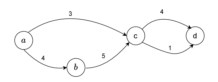
Figure 1: Example to illustrate the non-Markovian property of the CRL.

Mathematical Formulation.

To model such a non-Markovian behavior, let $\pi(s_{t+1}\mid S_{t})$ denote the probability that the traveler chooses the next state $s_{t+1}$ conditional on a joint state $S_{t}=\{s_{0},\ldots,s_{t}\}$, which represents the historical path from the origin to state $s_{t}$. Due to the incorporation of constraints, the resulting decision process is no longer Markovian—the policy at state $s_{t}$ may depend on the entire trajectory up to $s_{t}$. We will discuss the non-Markovian property in more detail in the next section.

At each state $s_{t}$, the traveler chooses the next state $s_{t+1}$ by maximizing the following expected utility:

$$\mathbb{E}_{\epsilon}\left[\max_{s_{t+1}\in N(s_{t})}\left\{v(s_{t+1}\mid s_{t})+V(S_{t+1})+\mu\epsilon(s_{t+1})\right\}\right],$$

where $v(s_{t+1}\mid s_{t})$ denotes the immediate deterministic utility of moving from $s_{t}$ to $s_{t+1}$, $V(S_{t+1})$ is the expected utility from the joint state $S_{t+1}=S_{t}\cup\{s_{t+1}\}$ to the destination, and $\epsilon(s_{t+1})$ are i.i.d. Gumbel (Type I extreme value) distributed random utilities.

Under this assumption, the value function $V(S_{t})$ from the joint state $S_{t}$ is computed as:

$$V(S_{t})=\begin{cases}0,&\text{if }s_{t}=d\text{ and }c(S_{t})\leq\alpha\\ -\infty,&\text{if }C(S_{t})>\alpha,\\ \mu\ln\left(\sum_{s_{t+1}\in N(s_{t})}\exp\left(\frac{1}{\mu}\left[v(s_{t+1}\mid s_{t})+V(S_{t+1})\right]\right)\right),&\text{otherwise},\end{cases}$$ (1)

where $C(S_{t})$ is the accumulated cost along the path $S_{t}$, given by

$$C(S_{t})=\sum_{i=0}^{t-1}c(s_{i+1}\mid s_{i}),$$

and $\alpha$ is the upper bound on the allowable accumulated cost. Intuitively, when the cost exceeds this threshold, the value function becomes $-\infty$, ensuring that the corresponding choice probability becomes zero.

Given the value function, the choice probability is given by a MNL model:

$$\pi(s_{t+1}\mid S_{t})=\begin{cases}\frac{\exp\left(\frac{1}{\mu}(v(s_{t+1}\mid s_{t})+V(S_{t+1}))\right)}{\sum_{s\in N(s_{t})}\exp\left(\frac{1}{\mu}(v(s\mid s_{t})+V(S_{t}\cup\{s\}))\right)},&\text{if }s_{t+1}\in N(s_{t}),\\ 0,&\text{otherwise}.\end{cases}$$

Finally, given an observed path $\sigma=\{s_{0},\ldots,s_{T}\}$, the path probability under the constrained RL model is given by:

$$P(\sigma)=\prod_{t=0}^{T-1}\pi(s_{t+1}\mid S_{t}).$$

It can be seen that, under the value function defined above, at any state $S_{t}$, if there exist two candidate next states $s$ and $s^{\prime}$ such that the accumulated cost of transitioning to $s$ remains below the threshold $\alpha$, while the accumulated cost of transitioning to $s^{\prime}$ exceeds $\alpha$, then—as expected—the probability of choosing state $s^{\prime}$ will be zero. We formalize this observation in the following proposition:

Proposition 1

Let $S_{t}=\{s_{0},s_{1},\ldots,s_{t}\}$ denote a joint state (i.e., the historical path up to time $t$), and let the accumulated cost along this path be $C(S_{t})=\sum_{i=0}^{t-1}c(s_{i+1}\mid s_{i})$. Suppose there exists at least one feasible next state $s\in\mathcal{S}$ such that the total cost of transitioning from $s_{t}$ to $s$ remains within the allowed threshold, i.e., $C(S_{t})+c(s\mid s_{t})\leq\alpha$. Then, for any alternative next state $s^{\prime}\in\mathcal{S}$ such that the accumulated cost violates the threshold, i.e., $C(S_{t})+c(s^{\prime}\mid s_{t})>\alpha$, the probability of choosing $s^{\prime}$ is zero, that is, $\pi(s^{\prime}\mid S_{t})=0$. As a consequence, for any full path $\sigma=\{s_{0},s_{1},\ldots,s_{T}\}$, if there exists a sub-path $\sigma^{\prime}=\{s_{0},\ldots,s_{H}\}$ for some $H\leq T$ such that the accumulated cost along $\sigma^{\prime}$ exceeds the threshold $\alpha$, i.e., $\sum_{t=0}^{H-1}c(s_{t+1}\mid s_{t})>\alpha$, then the probability of the entire path $\sigma$ is zero, i.e., $P(\sigma)=0$.

Proof. The proof is straightforward. From the recursive formulation of the value function $V(S_{t})$, consider a state $s_{t}$. If there exists a successor state $s^{\prime}$ such that $C(S_{t})+c(s^{\prime}\mid s_{t})>\alpha,$ then the corresponding value function becomes $V(S_{t}\cup\{s^{\prime}\})=-\infty$. Consequently, the choice probability formulation in (1) implies that $\pi(s^{\prime}\mid S_{t})=0.$

Now, consider a path $\sigma=\{s_{0},s_{1},\ldots,s_{T}\}$. Suppose there exists a subpath $\sigma^{\prime}=\{s_{0},\ldots,s_{H}\}$ for some $H\leq T$ such that the accumulated cost along $\sigma^{\prime}$ exceeds the threshold $\alpha$, i.e., $\sum_{t=0}^{H-1}c(s_{t+1}\mid s_{t})>\alpha.$ In this case, there must exist an extended state $\widetilde{S}_{i}=\{s_{0},...,s_{i}\}$ for some $i\in\{0,\ldots,H-1\}$ such that $\pi(s_{i+1}\mid\widetilde{S}_{i})=0$. This implies that the probability of selecting the entire path $\sigma$ is zero, i.e. $P(\sigma)=0,$ which establishes the claim.  

The above proposition highlights an important implication of the model: for any path, if at any point along that path the accumulated cost exceeds the specified upper bound $\alpha$, then the probability of taking that path is exactly zero. This result is consistent with the real-world constraints observed in several application domains. For instance, in the EV routing example, a driver must ensure that the battery never depletes entirely along the journey. As such, the driver would never consider a path that would result in the energy level dropping to zero at any point along the way, which corresponds to a constraint violation and thus leads to zero path probability. Similarly, in the context of bike-sharing or bike rental systems, consider a policy where users are required to return the bike within 30 minutes before initiating a new rental; otherwise, they incur a substantial penalty (Tsushima et al., 2023). In this case, a traveler (or renter) would not consider any path that violates this time constraint at any moment along the route. The model naturally encodes such behavior: any path that violates the constraint, even temporarily, will be assigned zero probability and effectively ruled out from the consideration choice set of paths.

4.2 Illustrative Examples

We present some simple examples to illustrate the implications of the modeling framework discussed above.

Example 1: Route choice with travel time upper-bounds

The first scenario considers a route choice problem in which we assume that travelers will not consider invalid route whose travel times exceed a travel time upper-bound $\alpha$. This is a common case in real world: A taxi driver chooses a route to pick up customer on time, or a shipper plans to deliver packages before a deadline.

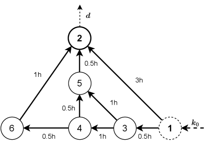
Figure 2: Toy network with travel times

We consider a toy network shown in Figure 2, where node $k_{0}$ is the origin and node $d$ is the destination. The number on each edge represents its travel time. The utility associated with each transition from node $s$ to node $s^{\prime}$ is computed as $v(s^{\prime}\mid s)=-2\times TT(s^{\prime}\mid s)$, where $TT(s^{\prime}\mid s)$ denotes the travel time from $s$ to $s^{\prime}$. The cost is also defined as the travel time on each edge, and we impose an upper bound $\alpha=2.5$, meaning that any path with a total travel time exceeding 2.5 hours will be assigned zero probability under the constrained model.

In Table 1, we report the path probabilities computed under both the original (unconstrained) RL model and the constrained RL model with $\alpha=2.5$. The values in parentheses represent the total travel time for each path. As observed, in the unconstrained setting, all paths have non-zero probabilities. In contrast, when the constraint is enforced, the probabilities of paths $[1,2]$ and $[1,3,4,6,2]$ become zero due to violation of the travel time limit.

No.	Path	$P(\sigma^{n})$
1	[1,2]	0.083
2	[1,3,5,2]	0.610
3	[1,3,4,5,2]	0.224
4	[1,3,4,6,2]	0.083

(a) Path probabilities given by the RL model without constraints

No.	Path	$P(\sigma^{n})$
1	[1,2] (3h)	0.000
2	[1,3,5,2] (2h)	0.731
3	[1,3,4,5,2] (2.5h)	0.269
4	[1,3,4,6,2] (3h)	0.000

(b) Path probabilities given by the constrained RL model

Table 1: Path choice probabilities given by the RL and constrained RL models.

4.3 Example 2: Route choice analysis for rechargeable vehicles

In the previous example, the costs represent travel times, which are always non-negative. In this section, we present a scenario where the cost can take both negative and positive values. Specifically, we consider a route choice problem for rechargeable vehicles that consume some form of energy (e.g., fuel or electricity) to operate. During long trips, such vehicles must periodically refuel or recharge at gas stations or charging stations.

In this scenario, certain locations in the network represent charging stations where a vehicle can replenish its energy up to a specified level in order to continue the trip. The cost function $c(s^{\prime}\mid s)$ represents the net energy change when transitioning from state $s$ to state $s^{\prime}$. Specifically, this cost takes a positive value when the vehicle travels along a road segment—corresponding to energy consumption—and a negative value when the vehicle visits a charging station—corresponding to energy replenishment. At the origin, the initial negative cost reflects the vehicle’s starting energy level. The energy constraint imposes that the accumulated cost at any point in time must remain less than or equal to the vehicle’s maximum energy capacity, denoted by $\alpha$. Formally, this is expressed as $C(S_{t})\leq\alpha$ for all time steps $t$. This condition ensures that the vehicle does not exceed its energy capacity and has sufficient energy to complete its journey.

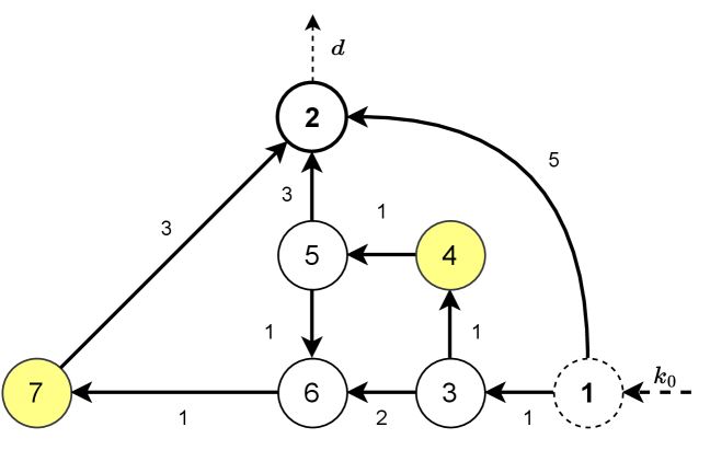
Figure 3: Toy network with charging stations.

We consider the toy network illustrated in Figure 3, which comprises 7 nodes and 10 links. The driver seeks to travel from the origin node $k_{0}$ to the destination node $d$. Each link is annotated with its travel time, and for simplicity, we assume that the travel time on a link is equal to the amount of energy consumed when traversing it. In this setting, Nodes 4 and 7 are designated as recharging stations. When the vehicle visits either of these nodes, the accumulated cost—representing the total energy consumed—is reset to zero, simulating a full recharge. We model the energy constraint by setting the initial energy level to zero, representing a fully charged vehicle at the start of the trip. Each traversal of a road link increases the accumulated cost (i.e., depletes energy), while visits to recharging stations reset this cost to zero, thereby allowing the vehicle to continue its journey without violating the energy constraint.

No.	Path	$P(\sigma)$ ($\alpha=5$)	$P(\sigma)$ ($\alpha=4$)	$P(\sigma)$ ($\alpha=3$)
1	[1,2]	0.644	0	0
2	[1,3,4,5,2]	0.237	0.665	0
3	[1,3,4,5,6,7,2]	0.032	0.090	1.000
4	[1,3,6,7,2]	0.087	0.245	0

Table 2: Path choice probabilities under different values of $\alpha$.

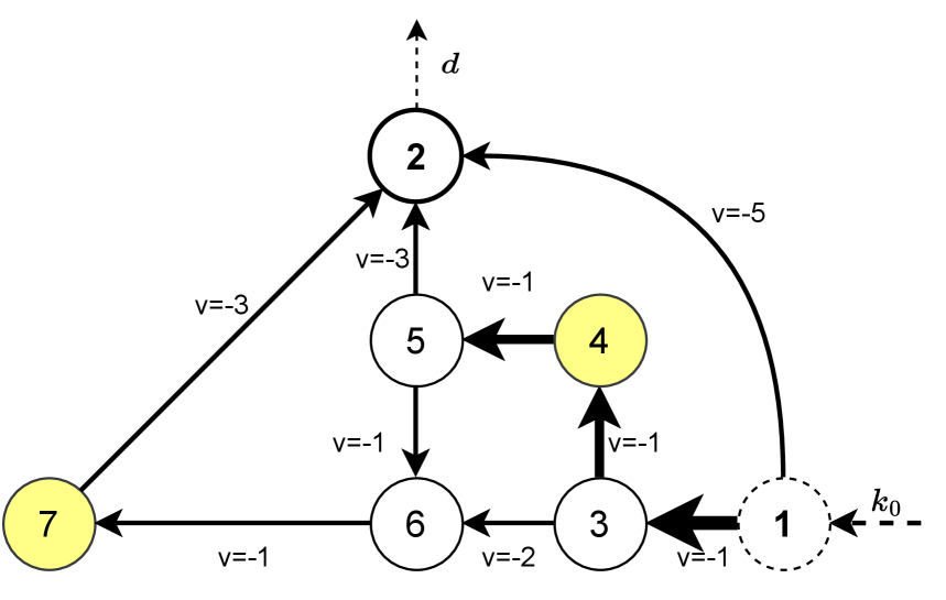
(a) $\alpha=5$

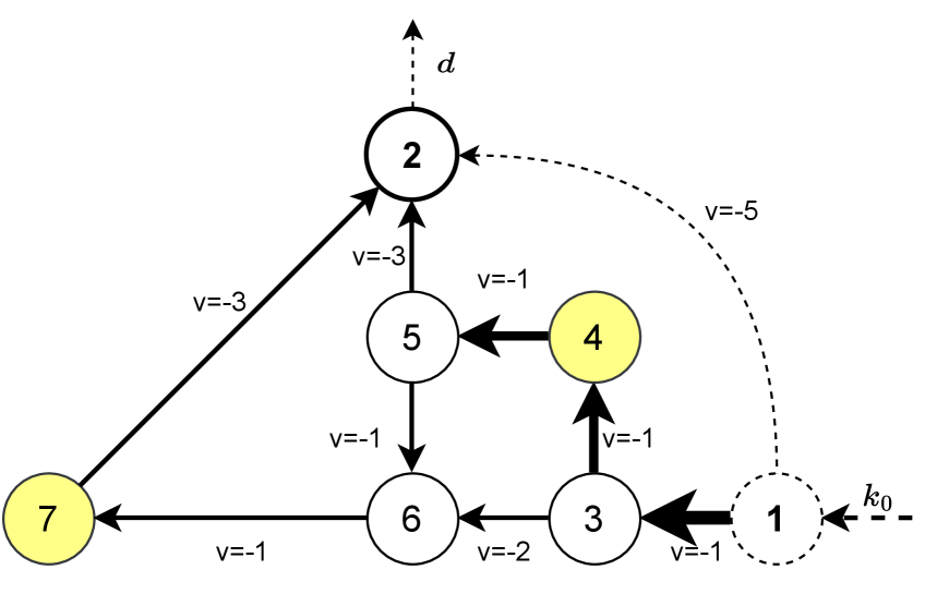
(b) $\alpha=4$

(c) $\alpha=3$

Figure 4: Visualization of path choice probabilities under varying energy thresholds $\alpha$.

Different values of the constraint parameter $\alpha$ lead to different sets of feasible paths. Intuitively, when $\alpha$ is high—corresponding to a vehicle with greater energy capacity—more paths become feasible and are included in the route choice set. In contrast, when $\alpha$ is low, the vehicle must visit charging stations more frequently to ensure it has sufficient energy to complete the trip. In the following, we illustrate how path choice probabilities vary with different values of $\alpha$, specifically $\alpha\in\{3,4,5\}$.

In Table 2, we report the path choice probabilities computed using the constrained Recursive Logit (RL) model under different energy thresholds $\alpha$. As observed, when $\alpha=5$, all candidate paths satisfy the energy constraint and are therefore feasible, resulting in strictly positive choice probabilities for all paths. However, as the threshold $\alpha$ decreases, some paths become infeasible due to excessive energy consumption without sufficient opportunity for recharging. Consequently, these paths receive zero probability under the constrained model. In particular, when $\alpha=3$, only a single path—namely $[1,3,4,5,6,7,2]$—remains feasible. This path includes both designated charging stations at Nodes 4 and 7, allowing the vehicle to replenish its energy and continue the trip under the energy constraint.

For visualization purposes, Figure 4 illustrates the path choice probabilities under three different values of the energy constraint parameter $\alpha$. The link utilities $v(s^{\prime}\mid s)$ are defined as $-2\times TT(s^{\prime}\mid s)$, where $TT(s^{\prime}\mid s)$ is the travel time between nodes $s$ and $s^{\prime}$. In the figure, dashed links represent transitions with zero probabilities under the constrained model, while the thickness of each solid link reflects the magnitude of its corresponding choice probability. For example, when $\alpha=5$, all links are feasible and thus have positive probabilities. Among them, the link $(1,3)$ has the highest probability of being chosen. Furthermore, at Node 3, the probability of transitioning to Node 4 (a charging station) is higher than the probability of transitioning to Node 6. In contrast, when $\alpha=3$, several links—including $(1,2)$, $(3,6)$, and $(5,2)$—have zero probability of being selected, as they lead to infeasible paths that violate the energy constraint. This visualization highlights how stricter energy constraints restrict the set of viable routes and alter the structure of the route choice probabilities accordingly.

It is important to highlight that $[1,3,4,5,6,7,2]$ is also the longest path in terms of travel time. This outcome underscores a critical insight: when energy constraints are in place, travelers may be forced to take longer routes in order to ensure sufficient energy availability, particularly through visits to charging stations. In contrast, in the unconstrained setting, this longest path receives the lowest choice probability due to its higher travel cost. This comparison demonstrates that ignoring operational constraints—such as energy limits—can result in significantly biased or incorrect predictions of route choice behavior. Incorporating such constraints into the modeling framework is therefore essential for producing realistic and reliable results.

4.4 Rechargeable vehicles in a grid network

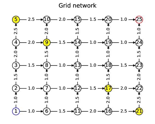
Figure 5: Grid graph with 25 nodes including 4 charging stations.

We now present a larger illustrative example to highlight the impact of feasibility constraints in route choice modeling for rechargeable vehicles. The network, shown in Figure 5, is a $5\times 5$ grid consisting of $25$ nodes, among which $4$ are designated as charging stations. A vehicle travels from node $1$ (bottom left) to node $25$ (top right). Each edge is associated with a travel time, and the instantaneous utility of traversing an edge is set to the negative of its travel time.

For the CRL model, we assume that the energy consumed on each link is equal to its travel time. The vehicle has a finite energy capacity of $\alpha=7$, meaning it must recharge at a station before the remaining energy is exhausted. This setting naturally enforces feasibility constraints: any route that exceeds the energy capacity without visiting a station is considered infeasible and is excluded from the consideration choice set.

We compute link choice probabilities under both the RL and CRL models using the specified link utilities. The resulting choice probability distributions are visualized by varying the thickness of the links in 6(a) and 6(b). In the RL model with an unrestricted choice set, links closer to the diagonal from node $1$ to node $25$ dominate, as they correspond to shorter travel times, whereas links farther away from the diagonal have lower probabilities.

In contrast, the CRL model with the energy upper-bound $\alpha=7$ yields drastically different probability patterns. Routes near the diagonal, which appear optimal under the RL model, become infeasible due to the absence of charging stations in that region and therefore disappear from the choice set. Instead, feasible routes that include detours to charging stations, often located near the corners, retain non-negligible probability mass. This result demonstrates how the CRL model successfully captures feasibility constraints that fundamentally alter the set of available alternatives, leading to more realistic modeling of traveler behavior in energy-constrained settings.

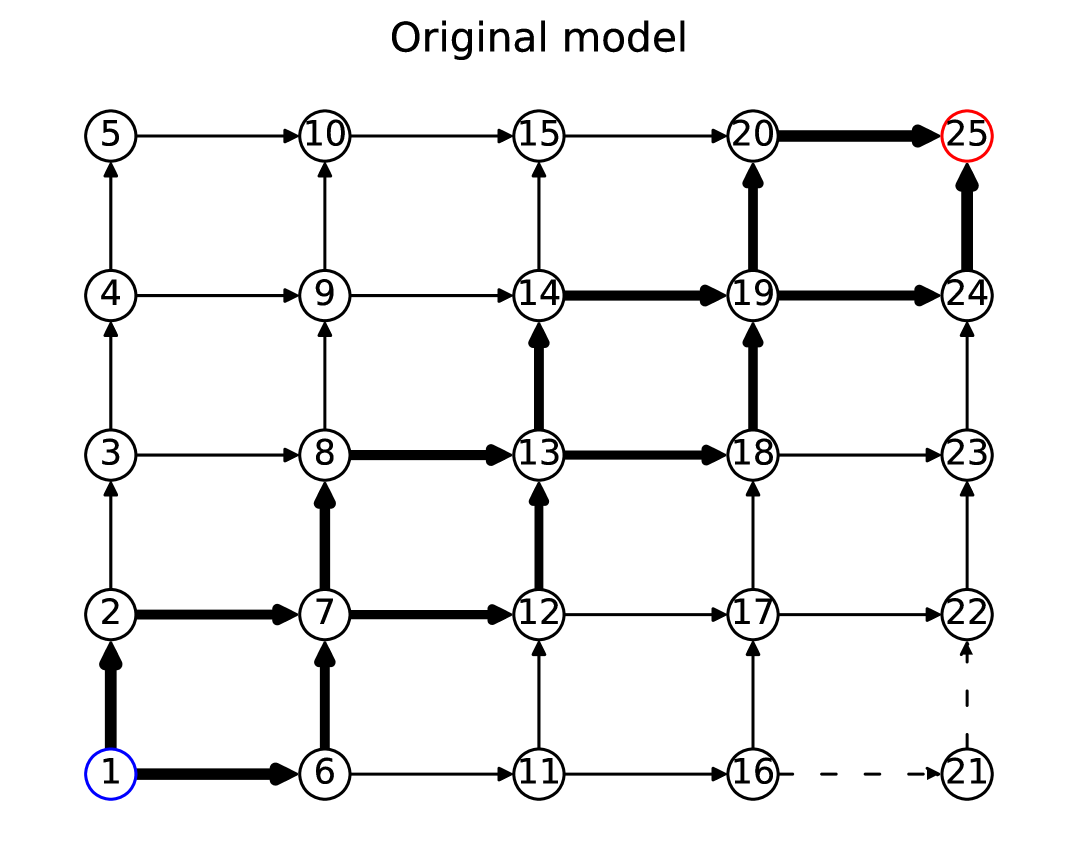
(a) Path probabilities in grid graph with unrestricted choice set.

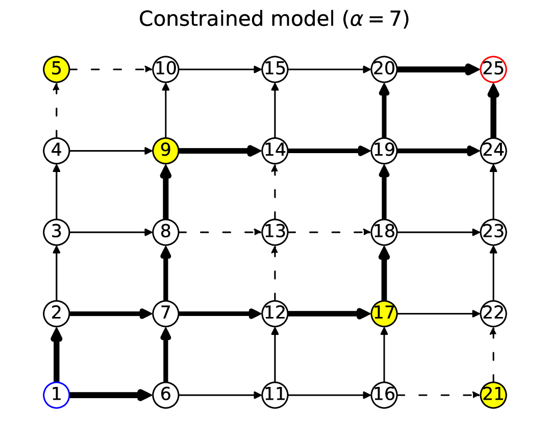
(b) Path probabilities in grid graph with energy constraint of $\alpha=7$.

Figure 6: Comparison of path probabilities in grid graph under (a) unrestricted choice set and (b) energy-constrained setting.

5 Model Properties

In this section we delve into the main properties of the CRL model described above.

5.1 Connection of Path-based MNL Models

First, to better understand the modeling formulation of the CRL model, let us connect it with a logit-based path choice model. It is well-known that the standard RL model is equivalent to the MNL model over the universal choice set of paths. That is, let $\Omega$ be the set of all possible paths reaching the destination $d$. The path choice probability given by the RL model can be expressed as:

$$P^{\text{\tiny RL}}(\tau)=\frac{e^{\frac{1}{\mu}v(\tau)}}{\sum_{\tau^{\prime}\in\Omega}e^{\frac{1}{\mu}v(\tau^{\prime})}},$$ (2)

where $v(\tau)$ is the accumulated utility of path $\tau$. Similarly, the proposition below shows that, if the cost $c(s^{\prime}|s)$ are non-negative, the CRL formulation gives path choice probabilities equivalent to an MNL model over a restricted universal choice set:

Proposition 2

Assume that $c(s^{\prime}|s)\geq 0$ for any $s,s^{\prime}\in{\mathcal{S}}$. Let $\Omega^{\alpha}$ be a restricted universal choice set that contains only paths whose cost does not exceed $\alpha$, i.e., $\Omega^{\alpha}=\{\tau\in\Omega~|~C(\tau)\leq\alpha\}$. Then, the CRL model is equivalent to the MNL model over $\Omega^{\alpha}$:

$$P^{\text{\tiny CRL}}(\tau)=\begin{cases}\frac{e^{\frac{1}{\mu}v(\tau)}}{\sum_{\tau^{\prime}\in\Omega^{\alpha}}e^{\frac{1}{\mu}v(\tau^{\prime})}}&\text{ if }\tau\in\Omega^{\alpha}\\ 0&\text{ otherwise }\end{cases}$$ (3)

where $v(\tau)$ is the accumulated utility along path $\tau$, i.e., for any path $\tau=\{s_{0},s_{1},\ldots,s_{T}\}$, $v(\tau)=\sum_{t=0}^{T-1}v(s_{t+1}|s_{t})$.

Proof. For any path $\tau=\{s_{0},s_{1},\ldots,s_{T}\}$, let $S_{t}=\{s_{0},\ldots,s_{t}\}$ denote the sequence of states from the origin $s_{0}$ up to state $s_{t}$. The choice probability of path $\tau$ under the CRL model can be computed as:

$$P(\tau) =\prod_{t=0}^{T-1}\pi(s_{t+1}\mid S_{t})$$

$$=\prod_{t=0}^{T-1}\frac{\exp\left(\frac{1}{\mu}(v(s_{t+1}\mid s_{t})+V(S_{t+1}))\right)}{\sum_{s\in N(s_{t})}\exp\left(\frac{1}{\mu}(v(s\mid s_{t})+V(S_{t}\cup\{s\}))\right)}$$

$$=\prod_{t=0}^{T-1}\frac{\exp\left(\frac{1}{\mu}(v(s_{t+1}\mid s_{t})+V(S_{t+1}))\right)}{\exp\left(\frac{1}{\mu}V(S_{t})\right)}$$

$$=\frac{\exp\left(\frac{1}{\mu}v(\tau)\right)}{\exp\left(\frac{1}{\mu}V(S_{0})\right)},$$ (4)

where $v(\tau)=\sum_{t=0}^{T-1}v(s_{t+1}\mid s_{t})$ is the total utility along path $\tau$, and $V(S_{0})$ is the value function at the origin.

The value function $V(S_{t})$ can be computed recursively using the following relation:

$$\exp\left(\frac{1}{\mu}V(S_{t})\right)=\begin{cases}1,&\text{if }s_{t}=d\text{ and }C(S_{t})\leq\alpha,\\ \sum\limits_{s_{t+1}\in N(s_{t})}e^{\frac{1}{\mu}v(s_{t+1}\mid s_{t})}\cdot e^{\frac{1}{\mu}V(S_{t}\cup\{s_{t+1}\})},&\text{if }s_{t}\neq d\text{ and }C(S_{t})\leq\alpha,\\ 0,&\text{otherwise},\end{cases}$$ (5)

for all $t=0,1,\ldots$, where $C(S_{t})$ is the accumulated cost (e.g., energy consumed) along the sequence $S_{t}$.

Moreover, assuming the cost function $c(s^{\prime}\mid s)$ is non-negative, it follows that for any two sequences $S_{h}\subseteq S_{k}$, if $C(S_{h})>\alpha$, then $C(S_{k})>\alpha$ as well. Consequently, if $V(S_{h})=-\infty$, then $V(S_{k})=-\infty$. As a result, the recursion simplifies to:

$$\exp\left(\frac{1}{\mu}V(S_{t})\right)=\sum_{s_{t+1}\in N(s_{t})}\exp\left(\frac{1}{\mu}v(s_{t+1}\mid s_{t})\right)\cdot\exp\left(\frac{1}{\mu}V(S_{t}\cup\{s_{t+1}\})\right),$$ (6)

for all $t$ such that $s_{t}\neq d$ and $C(S_{t})\leq\alpha$.

This implies:

$$\exp\left(\frac{1}{\mu}V(S_{0})\right)=\sum_{\tau\in\Omega}\exp\left(\frac{1}{\mu}v(\tau)\right)\cdot\exp\left(\frac{1}{\mu}V(\tau)\right),$$

where $\Omega$ denotes the set of all possible paths from $s_{0}$ to the destination $d$, and $V(\tau)$ is the value associated with the terminal state sequence of path $\tau$. Notably, $\exp\left(\frac{1}{\mu}V(\tau)\right)=0$ if $C(\tau)>\alpha$, and $\exp\left(\frac{1}{\mu}V(\tau)\right)=1$ if $C(\tau)\leq\alpha$. This leads to the final expression:

$$\exp\left(\frac{1}{\mu}V(S_{0})\right)=\sum_{\tau\in\Omega^{\alpha}}\exp\left(\frac{1}{\mu}v(\tau)\right),$$

where $\Omega^{\alpha}\subseteq\Omega$ is the set of all feasible paths satisfying the constraint $C(\tau)\leq\alpha$, as desired.  

We note that Proposition 2 no longer holds if the cost function is allowed to take both positive and negative values. The reason is that when $c(s^{\prime}\mid s)$ can be either positive or negative, the condition $C(\tau)\leq\alpha$ is not sufficient to guarantee the feasibility of a path $\tau$. In particular, even if the total accumulated cost along a path satisfies the constraint, the path may still be infeasible if, at any intermediate state $s_{t}$, the accumulated cost $C(S_{t})$ exceeds $\alpha$. This violates the per-step feasibility condition imposed by the constraint.

To extend Proposition 2 to the case where the cost function can take both positive and negative values, we refine the definition of the restricted choice set as follows:

Definition 1 (Feasible Path Set under Stepwise Constraint)

Let $\overline{\Omega}^{\alpha}$ denote the set of all paths from the origin to the destination such that, for every path $\tau\in\overline{\Omega}^{\alpha}$, the accumulated cost at every intermediate step does not exceed the threshold $\alpha$. Formally, we define:

$$\overline{\Omega}^{\alpha}=\left\{\tau=\{s_{0},\ldots,s_{T}\}\,\middle|\,s_{T}=d,~C(S_{t})\leq\alpha\text{ for all }S_{t}=\{s_{0},\ldots,s_{t}\},~t=0,\ldots,T\right\}.$$

Under this definition, we can show that the CRL model is also equivalent to a MNL model over the restricted choice set $\overline{\Omega}^{\alpha}$.

Proposition 3

The path probabilities induced by the CRL model are equivalent to those given by a MNL model defined over the restricted feasible set $\overline{\Omega}^{\alpha}$:

$$P^{\text{CRL}}(\tau)=\begin{cases}\frac{\exp\left(\frac{1}{\mu}v(\tau)\right)}{\sum\limits_{\tau^{\prime}\in\overline{\Omega}^{\alpha}}\exp\left(\frac{1}{\mu}v(\tau^{\prime})\right)}&\text{if }\tau\in\overline{\Omega}^{\alpha},\\ 0&\text{otherwise}.\end{cases}$$ (7)

Proof. We begin by leveraging the recursive formulation from Equation 6, which remains valid even when the cost function may take negative values:

$$\exp\left(\frac{1}{\mu}V(S_{t})\right)=\sum_{s_{t+1}\in N(s_{t})}\exp\left(\frac{1}{\mu}v(s_{t+1}\mid s_{t})\right)\cdot\exp\left(\frac{1}{\mu}V(S_{t}\cup\{s_{t+1}\})\right),$$

where $V(S_{t})$ denotes the value function at state $S_{t}$, and $N(s_{t})$ denotes the set of next feasible nodes from $s_{t}$.

Importantly, whenever the accumulated cost $c(S_{t})>\alpha$, we have: $\exp\left(\frac{1}{\mu}V(S_{t})\right)=0.$ Therefore, the total value function at the origin state $S_{0}$ becomes:

$$\exp\left(\frac{1}{\mu}V(S_{0})\right)=\sum_{\tau\in\Omega}\exp\left(\frac{1}{\mu}v(\tau)\right)\cdot\Psi(\tau),$$

where the weight function $\Psi(\tau)$ is computed as:

$$\Psi(\tau)=\begin{cases}0&\text{if there exists a subsequence }S^{\prime}\subseteq\tau\text{ such that }c(S^{\prime})>\alpha,\\ \exp\left(\frac{1}{\mu}V(\tau)\right)&\text{otherwise}.\end{cases}$$

As a result, only paths in the restricted feasible set $\overline{\Omega}^{\alpha}$ contribute to the sum, yielding:

$$\exp\left(\frac{1}{\mu}V(S_{0})\right)=\sum_{\tau\in\overline{\Omega}^{\alpha}}\exp\left(\frac{1}{\mu}v(\tau)\right).$$

Finally, combining this with the probabilistic formulation in Equation 4, we obtain the desired result:

$$P^{\text{CRL}}(\tau)=\frac{\exp\left(\frac{1}{\mu}v(\tau)\right)}{\sum\limits_{\tau^{\prime}\in\overline{\Omega}^{\alpha}}\exp\left(\frac{1}{\mu}v(\tau^{\prime})\right)}.$$

 

A direct implication of Proposition 3 is that, for any given path $\tau\in\overline{\Omega}^{\alpha}$, the path choice probability assigned by the original RL model is less than or equal to that assigned by the CRL model. As a result, the in-sample log-likelihood under the CRL model is always greater than or equal to that under the standard RL model. We formally state this result in the following corollary.

Corollary 1

For any feasible path $\tau\in\overline{\Omega}^{\alpha}$, we have $P^{\text{RL}}(\tau)\leq P^{\text{CRL}}(\tau).$ Consequently, given a dataset of observed trajectories $\mathcal{D}=\{\tau_{1},\ldots,\tau_{n}\}$, if all observed paths satisfy the constraint (i.e., $\tau_{i}\in\overline{\Omega}^{\alpha}$ for all $i$), then the CRL model yields a log-likelihood value that is greater than or equal to that of the RL model:

$$\mathcal{L}^{\text{CRL}}(\mathcal{D})\geq\mathcal{L}^{\text{RL}}(\mathcal{D}),$$

where the log-likelihood functions are defined as

$$\mathcal{L}^{\text{RL}}(\mathcal{D})=\sum_{\tau\in\mathcal{D}}\ln P^{\text{RL}}(\tau),\quad\mathcal{L}^{\text{CRL}}(\mathcal{D})=\sum_{\tau\in\mathcal{D}}\ln P^{\text{CRL}}(\tau).$$

The corollary follows directly from the fact that the restricted choice set $\overline{\Omega}^{\alpha}$ is a subset of the universal choice set $\Omega$, which immediately implies:

$$\sum_{\tau\in\overline{\Omega}^{\alpha}}\exp\left(\frac{1}{\mu}v(\tau)\right)\leq\sum_{\tau\in\Omega}\exp\left(\frac{1}{\mu}v(\tau)\right).$$

This inequality directly leads to the result $P^{\text{RL}}(\tau)\leq P^{\text{CRL}}(\tau)$ for any feasible path $\tau\in\overline{\Omega}^{\alpha}$. Equality holds, i.e., $P^{\text{RL}}(\tau)=P^{\text{CRL}}(\tau)$ for all $\tau$, if and only if the restricted and universal choice sets are identical, that is, $\overline{\Omega}^{\alpha}=\Omega$. In this case, all paths are feasible with respect to the constraint, and the CRL model reduces to the standard RL model. In fact, we can see that the inequality above is strict if the universal choice set $\Omega$ strictly contains the feasible set $\overline{\Omega}^{\alpha}$, i.e., $\mathcal{L}^{\text{CRL}}(\mathcal{D})>\mathcal{L}^{\text{RL}}(\mathcal{D}),$ whenever there exists a path $\tau\in\Omega$ that is not feasible with respect to the constraint ($\tau\notin\overline{\Omega}^{\alpha}$).

6 Markovian Choice Probabilities through Extended MDP

As discussed above, the CRL model is inherently non-Markovian, since the choice probabilities at a given state (i.e., a node in the network) depend not only on the current state but also on the sequence of historical states visited. This violation of the Markov property renders the model impractical for estimation and prediction. To address this issue, in the following section we propose an approach based on state-space expansion. The key idea is to augment the state representation with the information regarding the accumulated cost, thereby transforming the CRL model into an equivalent Markovian model. Once the Markov property is restored, the problem can be reformulated as a standard RL model, enabling efficient estimation through classical methods such as value iteration. We begin by presenting our approach to transform the model into a Markovian form, followed by a discussion of the associated estimation methods.

6.1 Markovian Choice Probabilities

To achieve Markovian choice probabilities, we leverage the observation that the expected utility at a state $s_{t}$ depends only on the accumulated cost at that state, rather than on the entire history of previously visited states. This motivates us to incorporate the accumulated cost into the state representation, thereby ensuring that the value function is independent of the historical trajectory.

Formally, we define an extended state space $\widetilde{\mathcal{S}}$, where each extended state $\widetilde{s}\in\widetilde{\mathcal{S}}$ is a pair $\widetilde{s}=(s,z),$ with $s\in\mathcal{S}$ denoting the original state and $z\in\mathbb{R}$ the accumulated cost up to that state. Similarly, we define the set of feasible next states in the extended space as

$$\widetilde{N}(\widetilde{s})=\bigl\{(s^{\prime},z^{\prime})\;\big|\;s^{\prime}\in N(s),\;z^{\prime}=z+c(s^{\prime}\mid s)\bigr\},$$

that is, each successor in the extended state space consists of a next state $s^{\prime}$ from the original state space together with the updated accumulated cost $z^{\prime}=z+c(s^{\prime}|s)$.

We now formulate a RL model on this extended state space. At each extended state $\widetilde{s}_{t}=(s_{t},z_{t})$, the decision-maker selects the next state $\widetilde{s}_{t+1}=(s_{t+1},z_{t+1})$ by maximizing the expected utility

$$\mathbb{E}_{\epsilon}\left[\max_{\widetilde{s}_{t+1}\in\widetilde{N}(\widetilde{s}_{t})}\Bigl\{\widetilde{v}(\widetilde{s}_{t+1}\mid\widetilde{s}_{t})+\widetilde{V}(\widetilde{s}_{t+1})+\mu\,\epsilon(\widetilde{s}_{t+1})\Bigr\}\right],$$

where $\widetilde{v}(\widetilde{s}_{t+1}\mid\widetilde{s}_{t})$ denotes the deterministic immediate utility of moving from $\widetilde{s}_{t}$ to $\widetilde{s}_{t+1}$, given by

$$\widetilde{v}(\widetilde{s}_{t+1}\mid\widetilde{s}_{t})=v(s_{t+1}\mid s_{t}),$$

$\widetilde{V}(\widetilde{s}_{t+1})$ is the expected utility value from the extended state $\widetilde{s}_{t+1}$ to the destination, and $\epsilon(\widetilde{s}_{t+1})$ are i.i.d. Gumbel-distributed (Type I extreme value) random components.

The value function $\widetilde{V}(\widetilde{s}_{t})$ associated with state $\widetilde{s}_{t}=(s_{t},z_{t})$ is defined recursively as

$$\widetilde{V}(\widetilde{s}_{t})=\begin{cases}0,&\text{if }s_{t}=d\text{ and }z_{t}\leq\alpha,\\[6.0pt] -\infty,&\text{if }z_{t}>\alpha,\\[6.0pt] \mu\ln\left(\sum_{\widetilde{s}_{t+1}\in\widetilde{N}(\widetilde{s}_{t})}\exp\!\left(\tfrac{1}{\mu}\bigl[\widetilde{v}(\widetilde{s}_{t+1}\mid\widetilde{s}_{t})+\widetilde{V}(\widetilde{s}_{t+1})\bigr]\right)\right),&\text{otherwise}.\end{cases}$$ (8)

In other words, the value function is assigned $-\infty$ whenever the accumulated cost at the current state exceeds the upper bound $\alpha$. In all other cases, it takes the standard log-sum-exp form of the RL model. This construction ensures that any path whose cumulative cost violates the constraint is rendered infeasible and, consequently, is assigned zero probability of being chosen in the decision process. In effect, the extended state-space formulation enforces the feasibility constraints directly within the recursive structure of the value function, thereby integrating the constraint into the Markovian dynamics of the model.

The choice probability at each state is given by the standard MNL model:

$$\widetilde{\pi}\bigl(\widetilde{s}_{t+1}\mid\widetilde{s}_{t}\bigr)=\begin{cases}\dfrac{\exp\!\left(\tfrac{1}{\mu}\left[\widetilde{v}(\widetilde{s}_{t+1}\mid\widetilde{s}_{t})+\widetilde{V}(\widetilde{s}_{t+1})\right]\right)}{\sum\limits_{\widetilde{s}\in\widetilde{N}(\widetilde{s}_{t})}\exp\!\left(\tfrac{1}{\mu}\left[\widetilde{v}(\widetilde{s}\mid\widetilde{s}_{t})+\widetilde{V}(\widetilde{s})\right]\right)},&\text{if }\widetilde{s}_{t+1}\in\widetilde{N}(\widetilde{s}_{t}),\\[12.0pt] 0,&\text{otherwise}.\end{cases}$$ (9)

For notational convenience, we denote the recursive logit model defined on the extended state space by ERL. We are now ready to state the main result, which establishes the equivalence between the ERL and the CRL model.

Theorem 2

The ERL model is equivalent to the CRL model described in Section 4, in the sense that for any path $\tau$ in the original state space $\mathcal{S}$, there exists a one-to-one mapping to a path $\widetilde{\tau}$ in the extended state space such that their choice probabilities coincide:

$$P^{\text{\tiny CRL}}(\tau)\;=\;P^{\text{\tiny ERL}}(\widetilde{\tau}).$$

Proof. The proof proceeds by showing that both probability formulations can be expressed as path-based probabilities over a restricted universal choice set. As established in Proposition 3, the CRL model assigns the following probability to a path $\tau$:

$$P^{\text{\tiny CRL}}(\tau)=\begin{cases}\dfrac{\exp\!\left(\tfrac{1}{\mu}v(\tau)\right)}{\sum\limits_{\tau^{\prime}\in\overline{\Omega}^{\alpha}}\exp\!\left(\tfrac{1}{\mu}v(\tau^{\prime})\right)},&\text{if }\tau\in\overline{\Omega}^{\alpha},\\[12.0pt] 0,&\text{otherwise},\end{cases}$$ (10)

where $v(\tau)$ denotes the total utility along path $\tau$, $\overline{\Omega}^{\alpha}$ is the restricted universal choice set under the cost constraint.

Now consider any path $\tau=[s_{0},\ldots,s_{T}]$ in the original state space. This path uniquely corresponds to a path in the extended state space,

$$\widetilde{\tau}=[\widetilde{s}_{0},\ldots,\widetilde{s}_{T}]\;\stackrel{{\scriptstyle\text{def}}}{{=}}\;[(s_{0},z_{0}),\ldots,(s_{T},z_{T})],$$

where $z_{0}=0$ and, for $t=1,\ldots,T$, the accumulated cost is defined recursively as

$$z_{t}=\sum_{k=0}^{t-1}c(s_{k+1}\mid s_{k}).$$

For notational clarity, let $\mathcal{C}(\widetilde{s})$ denote the accumulated cost associated with an extended state $\widetilde{s}$, i.e., $\mathcal{C}(\widetilde{s}_{t})=z_{t}$. The probability of $\widetilde{\tau}$ under the ERL model is given by the recursive logit formulation:

$$P^{\text{\tiny ERL}}(\widetilde{\tau})=\frac{\exp\!\left(\tfrac{1}{\mu}\sum_{t=0}^{T-1}\widetilde{v}(\widetilde{s}_{t+1}\mid\widetilde{s}_{t})\right)}{\exp\!\left(\tfrac{1}{\mu}\widetilde{V}(\widetilde{s}_{0})\right)}.$$

From the recursive definition of the extended value function, we have

$$\exp\!\left(\tfrac{1}{\mu}\widetilde{V}(\widetilde{s}_{t})\right)=\sum_{\widetilde{s}_{t+1}\in\widetilde{N}(\widetilde{s}_{t})}\exp\!\left(\tfrac{1}{\mu}\widetilde{v}(\widetilde{s}_{t+1}\mid\widetilde{s}_{t})\right)\exp\!\left(\tfrac{1}{\mu}\widetilde{V}(\widetilde{s}_{t+1})\right),$$

whenever $\mathcal{C}(\widetilde{s}_{t})\leq\alpha$, and $\exp(\tfrac{1}{\mu}\widetilde{V}(\widetilde{s}_{t}))=0$ otherwise. Iterating this recursion yields

$$\exp\!\left(\tfrac{1}{\mu}\widetilde{V}(\widetilde{s}_{0})\right)=\sum_{\widetilde{\tau}\in\widetilde{\Omega}}\exp\!\left(\tfrac{1}{\mu}\widetilde{v}(\widetilde{\tau})\right)\Psi(\widetilde{\tau}),$$

where $\widetilde{v}(\widetilde{\tau})=\sum_{(s,s^{\prime})\in\tau}\widetilde{v}(s^{\prime}\mid s)$ and $\Psi(\widetilde{\tau})$ is an indicator function, equal to $0$ if there exists any $\widetilde{s}\in\widetilde{\tau}$ with $\mathcal{C}(\widetilde{s})>\alpha$, and $1$ otherwise. Accordingly, we may equivalently restrict the summation to the feasible path set:

$$\widetilde{\Omega}^{\alpha}=\left\{\widetilde{\tau}\in\widetilde{\Omega}\;\middle|\;\mathcal{C}(\widetilde{s})\leq\alpha,\;\;\forall\widetilde{s}\in\widetilde{\tau}\right\},$$

so that

$$\exp\!\left(\tfrac{1}{\mu}\widetilde{V}(\widetilde{s}_{0})\right)=\sum_{\widetilde{\tau}\in\widetilde{\Omega}^{\alpha}}\exp\!\left(\tfrac{1}{\mu}\widetilde{v}(\widetilde{\tau})\right).$$

Therefore, the ERL path probability takes the form

$$P^{\text{\tiny ERL}}(\widetilde{\tau})=\frac{\exp\!\left(\tfrac{1}{\mu}\sum_{t=0}^{T-1}\widetilde{v}(\widetilde{s}_{t+1}\mid\widetilde{s}_{t})\right)}{\sum\limits_{\widetilde{\tau}\in\widetilde{\Omega}^{\alpha}}\exp\!\left(\tfrac{1}{\mu}\widetilde{v}(\widetilde{\tau})\right)}.$$

Finally, note that for the corresponding original path $\tau=[s_{0},\ldots,s_{T}]$, we have

$$\sum_{t=0}^{T-1}\widetilde{v}(\widetilde{s}_{t+1}\mid\widetilde{s}_{t})=\sum_{t=0}^{T-1}v(s_{t+1}\mid s_{t}).$$

Thus, the two path probabilities coincide:

$$P^{\text{\tiny ERL}}(\widetilde{\tau})\;=\;P^{\text{\tiny CRL}}(\tau),$$

establishing the desired equivalence.  

Theorem 2 establishes the equivalence between the non-Markovian CRL model and the Markovian ERL model. This equivalence is crucial, as it implies that estimation can be carried out on the extended state space using standard recursive logit estimation techniques, such as the NFXP algorithm (Rust, 1987b). In the following, we provide a detailed discussion of the estimation procedure for the ERL model. In particular, we highlight an important property: under certain conditions, estimation based on the ERL formulation exhibits greater numerical stability compared to estimation of an unconstrained RL model. This stability arises because the ERL representation naturally enforces feasibility constraints through the extended state space, thereby eliminating infeasible paths and reducing irregularities in the likelihood function.

6.2 Estimation Methods

Since the ERL model takes the standard form of the RL model, its estimation can be carried out using the NFXP algorithm. In this approach, value iteration is employed to compute both the value function $\widetilde{V}(\widetilde{s})$ and the corresponding likelihood function. To make estimation computationally feasible, we impose an additional assumption on the cost structure. Specifically, we assume that the cost $c(s^{\prime}\mid s)$ takes values in a discrete set. This assumption guarantees that the extended state space $\widetilde{\mathcal{S}}$ is finite and discrete, thereby enabling practical implementation of the NFXP algorithm on the ERL model.

The recursive definition of $\widetilde{V}(\widetilde{s})$ in (8) allows us to define

$$\widetilde{Z}(\widetilde{s})\;=\;\exp\!\left(\tfrac{1}{\mu}\widetilde{V}(\widetilde{s})\right),$$

and rewrite the Bellman recursion in terms of $\widetilde{Z}(\cdot)$ as

$$\widetilde{Z}(\widetilde{s})=\begin{cases}1,&\text{if }\mathcal{N}(\widetilde{s})=d\text{ and }\mathcal{C}(\widetilde{s})\leq\alpha,\\[6.0pt] 0,&\text{if }\mathcal{C}(\widetilde{s})>\alpha,\\[6.0pt] \sum\limits_{\widetilde{s}^{\prime}\in\widetilde{N}(\widetilde{s})}\exp\!\left(\tfrac{1}{\mu}\widetilde{v}(\widetilde{s}^{\prime}\mid\widetilde{s})\right)\cdot\widetilde{Z}(\widetilde{s}^{\prime}),&\text{otherwise},\end{cases}$$

where $\mathcal{N}(\widetilde{s})$ denotes the original state $s\in\mathcal{S}$ corresponding to the extended state $\widetilde{s}$.

Equivalently, we may encode this system in matrix form. First, for any state $\widetilde{s}$ such that $\mathcal{C}(\widetilde{s})>\alpha$, we set $\widetilde{N}(\widetilde{s})=\emptyset$, effectively removing infeasible states from the recursion. Then we define a vector $B\in\mathbb{R}^{|\widetilde{\mathcal{S}}|}$ with entries

$$B(\widetilde{s})=\begin{cases}1,&\text{if }\mathcal{N}(\widetilde{s})=d,\\ 0,&\text{otherwise},\end{cases}$$

and a nonnegative matrix $M\in\mathbb{R}^{|\widetilde{\mathcal{S}}|\times|\widetilde{\mathcal{S}}|}$ with elements

$$M(\widetilde{s},\widetilde{s}^{\prime})=\begin{cases}\exp\!\left(\tfrac{1}{\mu}\widetilde{v}(\widetilde{s}^{\prime}\mid\widetilde{s})\right),&\text{if }\widetilde{s}^{\prime}\in\widetilde{N}(\widetilde{s}),\\[6.0pt] 0,&\text{otherwise}.\end{cases}$$

With these definitions, the Bellman recursion can be written compactly as

$$\widetilde{Z}\;=\;M\widetilde{Z}+B,$$

which is a linear system of equations. This form can be solved efficiently via value iteration or directly through matrix inversion. Importantly, the system admits a unique solution under some certain conditions, as stated in the following proposition.

Proposition 4

Assume that the cost satisfies $c(s,s^{\prime})>0$ for all $s,s^{\prime}\in\mathcal{S}$. Then the matrix $(I-M)$ is invertible, where $I$ denotes the identity matrix (i.e., a diagonal matrix with ones on the main diagonal and zeros elsewhere). Consequently, the linear system $\widetilde{Z}=M\widetilde{Z}+B$ admits a unique solution, which can be written explicitly as $\widetilde{Z}=(I-M)^{-1}B.$

Proof. By construction, each entry $M(\widetilde{s},\widetilde{s}^{\prime})$ is strictly positive only if $\widetilde{s}^{\prime}\in\widetilde{N}(\widetilde{s})$, and in that case it is equal to $\exp(\tfrac{1}{\mu}\widetilde{v}(\widetilde{s}^{\prime}\mid\widetilde{s}))$. Since $c(s,s^{\prime})>0$ for all $(s,s^{\prime})$, the accumulated cost strictly increases along any path in the extended state space. This implies that no cycles can exist in the transition structure of $M$, as eventually the accumulated cost exceeds $\alpha$, forcing termination.

Hence, the matrix $M$ is strictly upper block-triangular after a suitable permutation of states, and its spectral radius satisfies $\rho(M)<1$. It follows that the Neumann series $(I-M)^{-1}=\sum_{k=0}^{\infty}M^{k}$ converges. Therefore, $(I-M)$ is invertible, and the linear system admits the unique solution $\widetilde{Z}=(I-M)^{-1}B.$  

An important implication of Proposition 4 is that the estimation of the CRL and ERL models can be carried out more conveniently compared to the original recursive logit (RL) model. Specifically, prior work has shown that the estimation of the RL model may suffer from instability when the utility function takes large values, which can render the associated Bellman equations infeasible (Mai and Frejinger, 2022). By contrast, Proposition 4 establishes that if the cost associated with each transition between states is strictly positive—a condition that is generally satisfied in practical applications—then the Bellman equations of the ERL model always admit a unique solution, regardless of the scale of the utility function $v(s^{\prime}\mid s)$. This property ensures that the ERL formulation avoids the degeneracies that may arise in the standard RL setting and thereby provides a stable foundation for consistent estimation.

7 Numerical experiments

In this section, we present a series of experiments to evaluate the effectiveness of the proposed CRL model in comparison with the standard RL model. The evaluation is carried out on both synthetic and real-world datasets. All experiments are conducted on a Google Cloud TPU v2-8 server equipped with a 96-core Intel Xeon 2.00 GHz CPU.

7.1 Analysis on Synthetic Networks and Datasets

We first conduct experiments on synthetic datasets in order to evaluate the performance of the proposed CRL model, compared to the standard RL model. Two problem settings of particular interest are considered:

1. Route choice with travel time upper bounds. In this setting, travelers are assumed to only consider routes whose total travel time does not exceed a pre-specified threshold. This reflects practical scenarios where travelers face strict deadlines, such as arriving on time for flights, meetings, or deliveries.

2. Route choice with rechargeable vehicles. Here, the traveler must ensure that the remaining battery energy of the vehicle never drops below zero along any chosen route. This captures important features of modern transportation systems where electric or hybrid vehicles are increasingly common, and route feasibility depends not only on travel time but also on energy availability.

Network generation.

For computational tractability, we construct synthetic networks in the form of directed acyclic graphs (DAGs). The DAGs are generated as random geometric graphs (Penrose, 2003), a topology frequently employed for benchmarking graph algorithms. In this setting, node locations are sampled uniformly at random within a unit square $[0,1]\times[0,1]$, and edges are created by connecting nodes whose Euclidean distance falls below a prescribed threshold. For each successive link, we associate four attributes—travel time, left turn, right turn, and U-turn—derived from the geometric positions of the incident nodes and their relative orientations. The travel time is proportional to the Euclidean length of the link, while turn indicators are determined from the angular relationship between consecutive links. This setup provides a controlled, yet flexible, framework for simulating route choice scenarios with heterogeneous link characteristics while maintaining a mathematically tractable network structure. To generate the observational data, we fix a ground-truth parameter vector $\beta=[-4,\;-0.1,\;-0.05,\;-0.3]^{\top}.$ We then simulate path choices according to the RL formulation.

Experimental setup.

The number of observations used for parameter estimation and in-sample prediction is set to $3000$, while an additional $1000$ observations are generated for out-of-sample prediction. Parameter estimation is conducted by maximizing the likelihood of the in-sample dataset, yielding estimated parameters $\beta^{*}$.

Evaluation metrics.

The quality of estimation is evaluated using log-likelihood measures. Given an observation dataset $\mathcal{D}=\{\tau_{1},\ldots,\tau_{n}\}$, we define the average log-likelihood under the estimated parameter vector $\beta^{*}$ as $\mathcal{L}^{RL}(\mathcal{D}\mid\beta^{*})=\frac{1}{n}\sum_{i=1}^{n}\ln P^{\text{\tiny RL}}(\tau_{i})$. Since log-likelihood values are always non-positive, values closer to zero indicate better alignment of the model with the observed data. Furthermore, to quantify the relative performance gain of CRL over RL, we further define the percentage improvement metric as:

$$\%Improve(\mathcal{D})=\frac{{\mathcal{L}}^{CRL}(\mathcal{D})-{\mathcal{L}}^{RL}(\mathcal{D})}{|{\mathcal{L}}^{RL}(\mathcal{D})|}\times 100\%.$$

A positive value of $\%Improve$ indicates that the CRL model achieves better performance (in terms of likelihood prediction) compared to the standard RL model.

The synthetic experiments enable us to systematically assess the effect of incorporating feasibility constraints (such as travel time thresholds or energy limits) into the choice model. In the standard RL formulation, unreasonable paths — for example, those that violate energy constraints or whose travel times far exceed practical limits — may still receive positive choice probabilities. This undesirable feature often results in biased parameter estimates and degraded predictive accuracy. By contrast, the CRL model explicitly removes infeasible paths from the universal choice set, ensuring that only feasible routes are considered in the estimation process. This leads to more robust parameter recovery and improved generalization capability. Consequently, the CRL model is expected to outperform the RL model when constraints are taken into consideration, in both for in-sample estimation and out-of-sample prediction

7.1.1 Route choice with travel time upper-bounds

In this experiment, we consider a route choice setting in which the traveler imposes an upper bound on the total travel time. The networks and associated observations are generated as follows.

Graph generation.

We construct directed acyclic graphs (DAGs) of varying sizes, specifically with $20$, $30$, $40$, and $50$ nodes. For each size, $5$ independent DAGs are generated using the random geometric graph method. More precisely, $N$ nodes are uniformly distributed within a $1\times 1$ geometric space. An edge is drawn between two nodes if their Euclidean distance is smaller than $\frac{2}{\sqrt{N}}$. Additional edges are added if necessary to ensure that the graph is connected. The node with the smallest index is designated as the source, the node with the largest index as the destination, and all edges are oriented from smaller to larger indices, thereby ensuring acyclicity.

Observation generation.

Let $T_{\max}$ denote the longest feasible travel time of any route from source to destination in a given DAG. The cost associated with each link is interpreted as the travel time on that edge. To impose feasibility, we introduce an upper bound $\alpha$ on the total travel time that a traveler is willing to accept, defined as $\alpha=\%threshold\times T_{\max},$ where $\%threshold$ is a parameter specifying the ratio of the upper bound relative to the longest possible route. We consider eight levels of $\%threshold$ ranging from $20\%$ to $90\%$.

Once $\alpha$ is specified, we generate route choice observations under two models:

• Recursive Logit (RL). Observations are generated using the standard RL model. For consistency with the imposed travel time constraint, we discard any path samples whose total travel time exceeds $\alpha$, as such routes are deemed unrealistic for the traveler.

• Constrained Recursive Logit (CRL). Observations are generated using the CRL formulation, where infeasible paths (i.e., with travel time greater than $\alpha$) are systematically excluded from the universal choice set.

Experimental protocol.

For each DAG and each $\%threshold$ setting, we conduct $10$ independent trials. In each trial, $3000$ in-sample and $1000$ out-of-sample route observations are generated. The estimated parameters obtained from the in-sample observations are then used to evaluate both in-sample and out-of-sample log-likelihood performance.

To quantify the improvement of CRL over RL, we compute the percentage improvement metric $\%Improve$ (defined in the previous section). For each configuration, the average $\%Improve$ across $10$ trials is reported. This provides a robust comparison of the two models across varying network sizes and travel time thresholds, highlighting the conditions under which the CRL model yields the largest performance gains.

Comparison results.

The estimation results obtained when the RL model is used to generate observations are shown in Figure 7. Out-of-sample results are almost indistinguishable from in-sample ones, indicating that both the observation size and the number of trials are sufficiently large to ensure consistent parameter estimation.

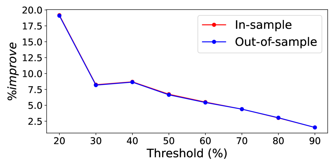
(a) 20 nodes

(b) 30 nodes

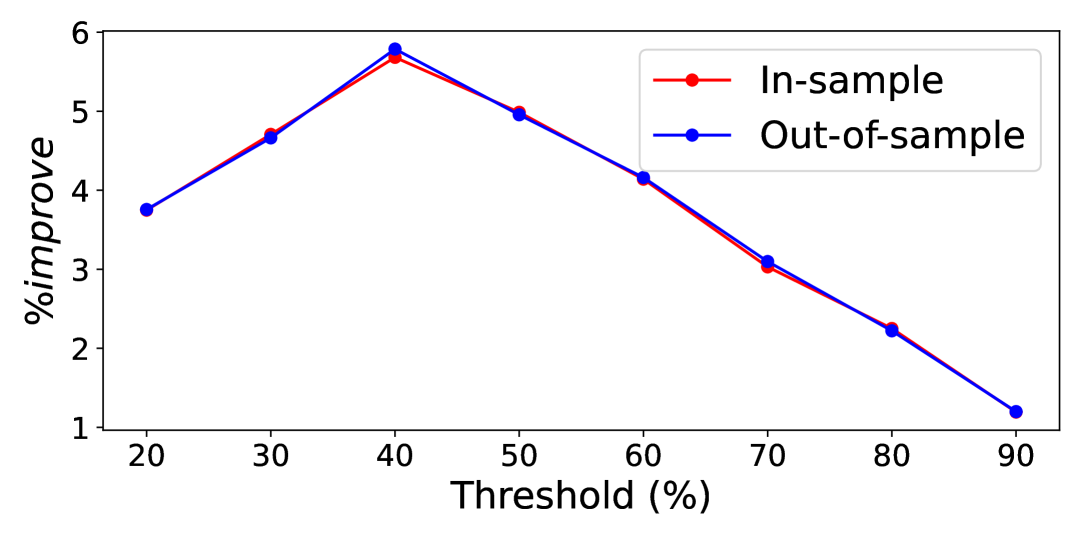
(c) 40 nodes

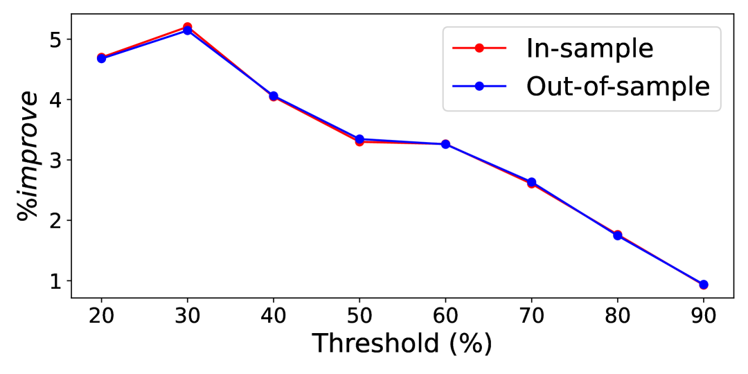
(d) 50 nodes

Figure 7: Estimation on synthetic observations generated by the RL model.

In terms of performance, the CRL model consistently achieves better (i.e., higher) log-likelihood values than the standard RL model. However, the performance gap between the two models decreases as the upper-bound threshold increases. This behavior is expected: when the threshold approaches $100\%$, nearly all routes remain feasible, and the CRL formulation reduces to the unconstrained RL model. Hence, under such conditions, the two models become virtually identical. At the other extreme, when the threshold is very tight (e.g., $20\%$ or $30\%$ of $T_{\max}$), the improvement of CRL over RL is less pronounced and even fluctuates across trials. This effect can be attributed to the limited number of feasible routes available under such strict constraints, which reduces the variability of the choice set and may cause instability in estimation.

When the observations are generated by the CRL model, the percentage improvements are reported in Figure 8. In this case, the downward trend of $\%Improve$ is more stable: the improvement decreases smoothly from approximately $8$–$10\%$ at $\%threshold=20\%$ to nearly $0\%$ at $\%threshold=90\%$. This confirms the expected behavior that, as the upper bound becomes less restrictive, the CRL and RL models converge to similar performance.

Another notable observation is that the performance gap between CRL and RL becomes less pronounced as the size of the DAG increases. This phenomenon is natural, since larger graphs imply exponentially larger route choice sets. With the number of observations fixed at $3000$, the sampled trajectories cover only a small fraction of the feasible choice set in larger graphs. As a result, the available data are less informative, and the distinction in performance between CRL and RL diminishes.

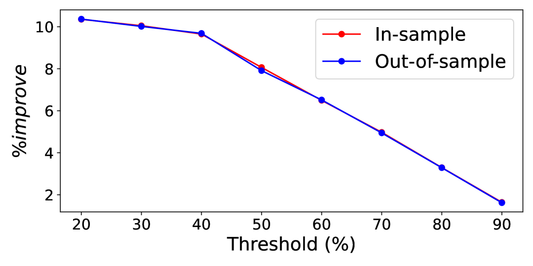
(a) 20 nodes

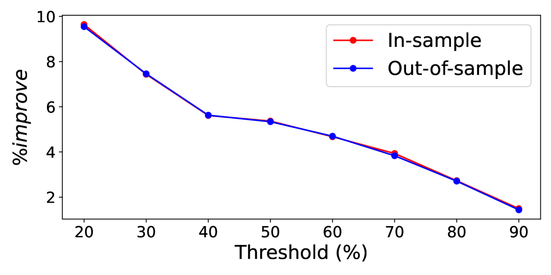
(b) 30 nodes

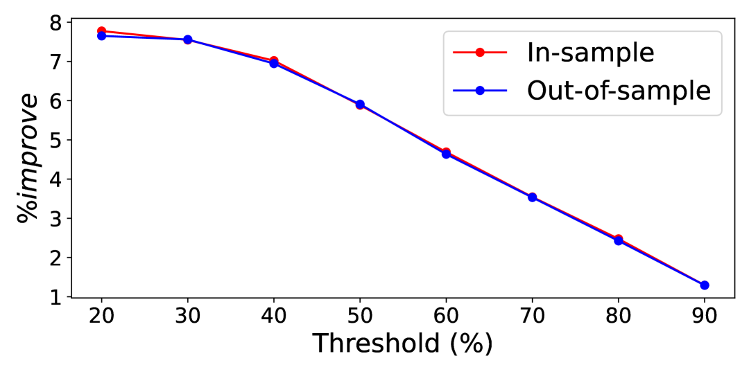
(c) 40 nodes

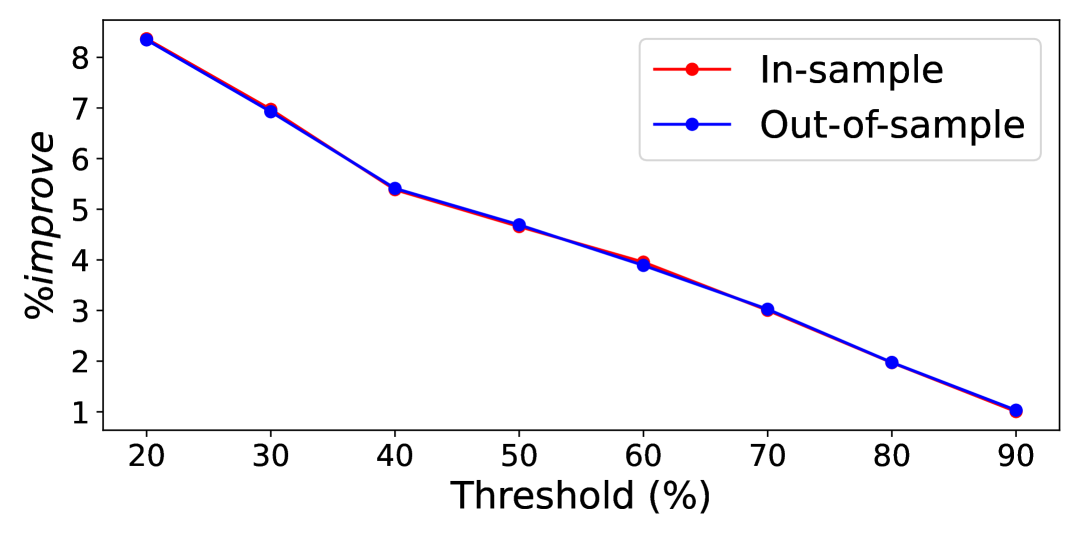
(d) 50 nodes

Figure 8: Estimation on synthetic observations generated by the CRL modes.

Taken together, these results demonstrate that the proposed CRL model offers estimation performance that is at least comparable to, and often better than, the standard RL model in the presence of upper-bound constraints. In particular, CRL better aligns with realistic travel behavior when such feasibility constraints are binding.

7.1.2 Route Choice for Rechargeable Vehicles

We next conduct experiments in a more challenging setting that incorporates an energy consumption constraint into the route choice behavior, mimicking the case of rechargeable vehicles. This setting is particularly relevant for modern transportation networks, where travelers must ensure that their remaining battery energy never falls below zero along the chosen route.

Graph generation.

As in the previous case, we generate DAGs with sizes ranging from $20$ to $50$ nodes. To simulate the availability of recharging infrastructure, a set of “stations” is randomly placed among the nodes of each graph. The number of stations is set to $10\%$ of the DAG size, reflecting the fact that only a limited fraction of nodes allow recharging.

Observation generation.

Since the standard RL model cannot simulate the action of fully recharging energy at stations (and thus cannot generate feasible trajectories under the energy constraint), we rely exclusively on the proposed CRL model to generate observations in this setting. This highlights an important strength of the CRL framework: its ability to naturally incorporate feasibility constraints into the path choice process. For each DAG size, we generate $5$ independent graph instances with randomly placed stations. For each instance, synthetic route choice data are generated under the CRL model.

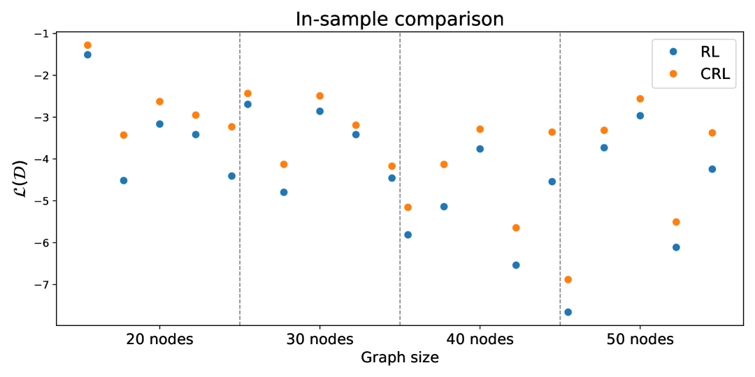
(a) In-sample

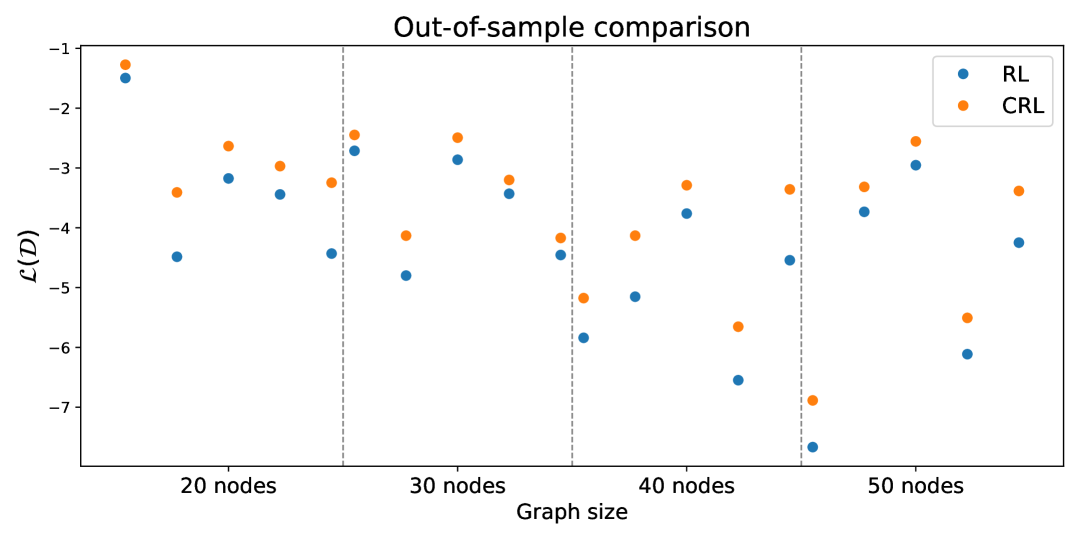
(b) Out-of-sample

Figure 9: In-sample and out-of-sample average log-likelihood comparisons for rechargeable vehicles.

Figure 9 reports the estimation errors of both RL and CRL in the energy-constrained setting. The performance gap between the two models is substantially larger here: CRL (orange dots) consistently outperforms RL (blue dots) across all graph sizes. The average improvements of CRL over RL for DAGs with $20$, $30$, $40$, and $50$ nodes are $21\%$, $10\%$, $17\%$, and $13\%$, respectively. This significant gain highlights the importance of explicitly modeling feasibility constraints. While the upper-bound constraint considered previously only limits the set of acceptable routes by travel time, the recharging constraint introduces a more intricate form of path feasibility that requires accounting for energy dynamics along the route. Since the standard RL model cannot capture this complexity, it misallocates probability mass to infeasible trajectories, leading to poorer estimation. By contrast, the CRL model systematically enforces the energy constraint through the extended state space, thereby yielding consistently higher likelihood values.

7.1.3 Estimation Time Comparison:

As discussed earlier, the CRL model entails higher computational requirements compared to the standard RL model. We now briefly examine this aspect. Figure 10 compares the estimation times of RL and CRL across different network sizes and threshold levels. For small networks (20–30 nodes), the estimation times of the two models are nearly identical, with both completing estimation in under two seconds across all threshold percentages. This suggests that the additional state-space expansion required by CRL does not impose a significant computational burden at modest network scales.

As the network size increases to 40 and 50 nodes, differences between the two models become more noticeable. While the RL model maintains nearly constant estimation times (around $0.4$–$0.6$ seconds), the CRL model exhibits increasing estimation times as the threshold percentage grows, reaching about $2.8$ seconds for the largest networks under the most relaxed constraints. This reflects the fact that CRL estimation must operate on an extended state space, whose size grows both with the number of nodes and with looser feasibility bounds.

Overall, these results highlight a trade-off: CRL ensures behavioral consistency by eliminating infeasible paths, but at the expense of increased computational burden in large and cyclic networks.

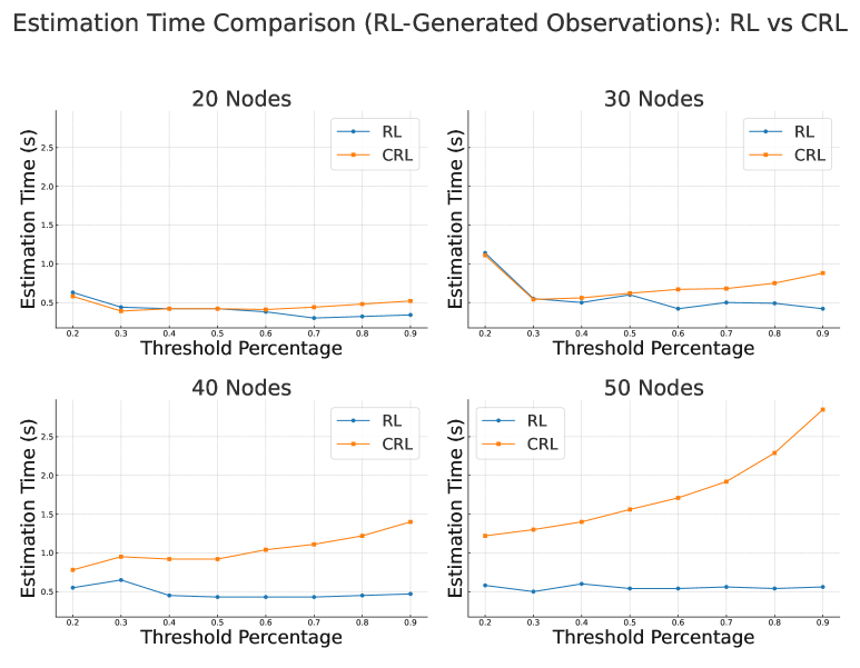
Figure 10: Estimation time comparison between RL and CRL on synthetic datasets across varying network sizes and threshold levels.

7.2 Experiments on Sioux Falls Network

Sioux Falls network.

In addition to synthetic datasets, we evaluate the proposed CRL model on the well-known Sioux Falls transportation network. Originally introduced by LeBlanc et al. (1975), this network has become a standard benchmark in the transportation science and operations research literature for testing traffic assignment and route choice models. The Sioux Falls network consists of $24$ nodes and $76$ directed links, together with an origin–destination (OD) demand matrix that specifies travel demand between selected node pairs. Each link is associated with a free-flow travel time and a capacity parameter, allowing link travel times to be modeled under congestion effects (e.g., using the Bureau of Public Roads function).

The Sioux Falls network is particularly attractive as a benchmark for route choice models because it strikes a balance between realism and tractability: it is large enough to capture meaningful network structure and route diversity, yet small enough to permit efficient computation of RL and CRL likelihoods. In our experiments, we use the Sioux Falls network to assess the practical applicability of the CRL model on a realistic network topology and to compare its performance against the standard RL model.

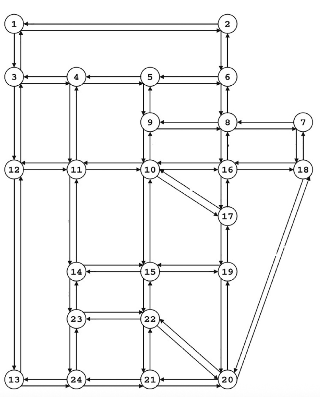
Figure 11: Sioux Falls network.

As mentioned in Section 6, one of the main advantages of the CRL model is that, under mild assumptions on the cost function, the Bellman equations always yield a unique solution. This solution can be computed efficiently either through value iterations or matrix inversion, thereby ensuring stable and efficient estimation. In contrast, as highlighted in (Mai and Frejinger, 2022), the original RL model often fails to produce reasonable parameter estimates, particularly in networks with many cycles. In such cases, the recursive structure of the Bellman equations may break down or lead to unstable likelihood evaluations. The Sioux Falls network provides a challenging testbed in this respect: its topology contains numerous cycles, making estimation under the standard RL model highly unstable.

The primary objective of this experiment is therefore to compare the estimation stability of RL and CRL on the Sioux Falls network. By evaluating performance on this benchmark, we can assess whether the CRL formulation indeed provides the robustness required for realistic networks with cyclic structures.

Observation generation.

Due to the failure of the RL model in estimation (as reported below), we rely on the CRL model to generate observations. In this setting, the cost function is specified as $c(s,s^{\prime})=1$ for every edge $(s,s^{\prime})$. This specification effectively imposes a constraint on the maximum number of edges that a traveler can traverse to reach the destination. Importantly, this choice satisfies the assumption stated in Section 6, and therefore guarantees that the value function can always be computed successfully.

Following the same experimental protocol as before, we generate $3000$ in-sample trajectories and $1000$ out-of-sample trajectories. The CRL model incorporates six attributes to simulate route choice probabilities: road capacity, road length, travel time, left turns, right turns, and U-turns. The associated parameter vector used for data generation is $\beta=[-0.5,\;0,\;1,\;-0.1,\;-0.05,\;-0.3]^{\top}.$ Note that since some of these coefficients are positive, certain arcs may yield positive utility values. This, in turn, can cause the unconstrained RL model to misbehave and fail during estimation, highlighting the necessity of the CRL framework for stable likelihood evaluation in such settings.

Table 3: Average log-likelihood values at estimation for the Sioux Falls dataset

$\alpha$ (upper bound on number of edges)	RL	CRL
10	–	-4.70
15	–	-11.69
20	–	-17.71
25	–	-23.90

The estimated average log-likelihood values for the two models are reported in Table 3. As shown, the RL model fails to return reasonable log-likelihood values across all experimental setups. This failure occurs because the solver is unable to compute the Bellman equations successfully in networks with many cycles, resulting in undefined values. We denote these unsuccessful cases by “-” in the table. In contrast, the CRL model can be estimated successfully in all settings. Furthermore, its estimation results exhibit a clear downward trend as the maximum number of edges allowed by the constraint $\alpha$ increases. When the choice set is very small (e.g., routes with no more than $10$ edges), the estimated log-likelihood values are relatively high. As $\alpha$ increases (e.g., allowing up to $25$ edges), the log-likelihood values decrease substantially. This behavior is intuitive: for a fixed number of observations, expanding the restricted universal choice set introduces many additional feasible paths, thereby lowering the probability assigned to any particular observed route.

These results illustrate two key insights. First, the CRL formulation provides a stable and feasible estimation procedure even in challenging cyclic networks such as Sioux Falls, where the original RL model completely fails. Second, the relationship between $\alpha$ and the log-likelihood reflects the natural trade-off between model flexibility (larger choice sets) and estimation sharpness (higher likelihood concentration on observed data).

7.3 Real-world Large-scale Traffic Network

In this section, we present a comparative analysis of estimation results for the RL and CRL models. The dataset employed is the same as that used in previous studies on route choice modeling (Fosgerau et al., 2013, Mai et al., 2015, 2018), collected in Borlänge, Sweden. The underlying network consists of $3077$ nodes and $7459$ links. Since the network is uncongested, link travel times can be treated as static and deterministic. The sample comprises $1832$ observed trips, each corresponding to a simple path containing at least five links. In total, the dataset covers $466$ destinations, $1420$ distinct origin–destination (OD) pairs, and more than $37{,}000$ link choices. The instantaneous utility function is given as follows:

$$v(a|k;\beta)=\beta_{TT}TT(a)+\beta_{LT}LT(a|k)+\beta_{LC}LC+\beta_{UT}UT(a|k)$$

in which $TT(a)$ is the travel time on link $a$, $LT(a|k)$ is a left turn dummy of the turn from link $k$ to $a$, $LC$ is a constant one value and $UT(a|k)$ is a u-turn dummy from $k$ to $a$.

Both RL and CRL are applied for in-sample estimation on the observation dataset. All experimental settings follow those in the original RL model publication (Fosgerau et al., 2013). In this experiment, the constraint incorporated by the CRL model is a bound constraint on the link count of each route, which is defined as the sum of the $LC$ attribute values over the links in the route. The distribution of link counts across the $1832$ observed routes is illustrated in Figure 12. The maximum number of links in a single route is $106$, which naturally serves as the upper bound for the constraint. It is important to note that link count is already a discrete variable, making it straightforward to apply the CRL model in this context. Moreover, as discussed in Section 6, the strict positivity of the cost values (here given by $LC$) ensures that the extended network is cycle-free. This property guarantees that the CRL model can be estimated efficiently using standard solution methods.

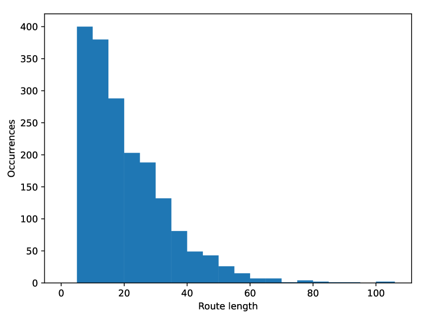
Figure 12: Distribution of link counts in the observation set.

Model	Property	Attributes				${\mathcal{L}}(\mathcal{D})$
		$TT$	$LC$	$LT$	$UT$
RL	$\widehat{\mathbf{\beta}}$	-2.49	-0.41	-0.93	-4.46	-3.44
	Std. Err.	0.07	0.01	0.03	0.10
	$t$-test(0)	-37.90	-39.58	-37.25	-45.39
CRL	$\widehat{\mathbf{\beta}}$	-2.51	-0.41	-0.93	-4.56	-3.39
	Std. Err.	0.07	0.01	0.03	0.10
	$t$-test(0)	-38.48	-37.38	-34.11	-45.05

Table 4: Estimation results on the Borlänge dataset.

The estimation results for both RL and CRL are reported in Table 4. Overall, the estimated parameters are very close across the two models, suggesting that both approaches capture the main behavioral patterns in the dataset. However, the CRL model achieves a slightly higher log-likelihood value ($-3.39$ compared to $-3.44$ for RL), corresponding to an improvement of approximately $1.5\%$ in the likelihood value.

We also apply a cross-validation approach to compare the prediction performance of RL and CRL. The full sample set is randomly split into two subsets: 80% of the observations are used for estimation, while the remaining 20% serve as a holdout set to assess predictive capability. In total, 30 different estimation–holdout partitions are generated. For each partition, we estimate the parameters on the estimation set and then compute the average log-likelihood on the holdout set using the estimated parameters. These predicted log-likelihood values across the 30 samples are shown in Figure 13, with the samples arranged in ascending order of RL’s prediction values for clarity. CRL consistently outperforms RL across all samples, with an average predicted log-likelihood of $-3.38$ compared to $-3.43$ for RL.

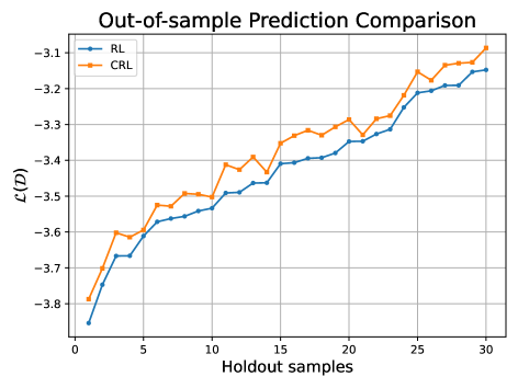
Figure 13: Average log-likelihood values over holdout samples for the Borlänge dataset.

This modest yet systematic improvement demonstrates that the CRL formulation is capable of capturing additional structural constraints in traveler behavior that are overlooked by the unconstrained RL model. It should be noted, however, that the magnitude of the improvement is relatively smaller compared to the case of synthetic data reported earlier. This is largely due to the fact that the Borlänge network is uncongested, so travelers are not strongly constrained by travel time or link count. As a result, paths with the shortest travel times dominate the choice probabilities, leaving limited scope for CRL to provide large gains over the unconstrained RL formulation. Nevertheless, even under such favorable conditions for RL, the CRL model still delivers consistent in-sample and out-of-sample improvements, underscoring its robustness in capturing feasibility conditions whenever they are present.

It is worth noting that the computational cost of CRL is substantially higher than that of RL (approximately $50\times$ higher for this real dataset). This increase reflects the added complexity of operating on the extended state space. Nevertheless, the improved model fit demonstrates that CRL provides significant value in situations where datasets involve constraints or atypical features that cannot be adequately captured by the standard RL model. Importantly, estimation remains feasible in practice: it can be completed in under ten hours, and further speedups are possible through parallel computing or decomposition techniques (Mai et al., 2018). These observations highlight the practical viability of CRL for large-scale, real-world datasets.

8 Conclusion

This paper introduced the CRL model, which extends the classical RL framework by explicitly incorporating feasibility constraints into the universal choice set. By enforcing that any path violating a constraint receives zero probability, the CRL model yields behaviorally consistent predictions while retaining the computational advantages of RL. We showed that estimation can be made tractable through a state-space extension, established equivalence to path-based MNL under restricted universal choice sets, and demonstrated extensions to multiple constraints and nested RL. Empirical results on both synthetic and real networks confirm that CRL provides more realistic predictions and stable estimation compared to RL, especially in cyclic networks. Future work may focus on improving computational efficiency of the extended state-space estimation for large-scale networks, as well as exploring relaxed formulations where infeasible paths are penalized rather than strictly excluded, thereby broadening the applicability of CRL in practical contexts.

Appendix

Appendix A Extension to Multiple-Constrained RL

We now extend the CRL framework to accommodate multiple constraints. Such a multi-constrained formulation generalizes the single-constraint CRL model to settings where several feasibility conditions must be satisfied simultaneously. For instance, an electric vehicle traveler may face both a travel-time deadline and a battery capacity limit, while a bike-sharing trip may be restricted by a maximum rental duration and station availability. The multi-constraint CRL framework incorporates these conditions directly into the recursive structure, preserving the Markovian property while systematically assigning zero probability to any path that violates one or more constraints.

As a starting point, we provide a formal definition of a feasible path in the context of multiple constraints.

Definition 3 (Feasible Path Set under Multiple Stepwise Constraints)

Let $\mathbf{c}(s,s^{\prime})=\bigl(c^{1}(s,s^{\prime}),\ldots,c^{K}(s,s^{\prime})\bigr)$ denote a $K$-dimensional vector of transition costs, and let $\boldsymbol{\alpha}=(\alpha_{1},\ldots,\alpha_{K})$ be the corresponding vector of upper bounds. For a path $\tau=\{s_{0},\ldots,s_{T}\}$, define the accumulated cost vector up to step $t$ as

$$\mathbf{C}(S_{t})=\left(\sum_{j=0}^{t-1}c^{1}(s_{j},s_{j+1}),~\ldots,~\sum_{j=0}^{t-1}c^{K}(s_{j},s_{j+1})\right),$$

where $S_{t}=\{s_{0},\ldots,s_{t}\}$ is the partial trajectory up to time $t$.

The feasible path set under multiple stepwise constraints is defined as

$$\widetilde{\Omega}^{\boldsymbol{\alpha}}=\left\{\tau=\{s_{0},\ldots,s_{T}\}~\middle|~s_{T}=d,~C^{k}(S_{t})\leq\alpha_{k}\;\;\forall k=1,\ldots,K,~\forall t=0,\ldots,T\right\}.$$

In words, a path $\tau$ is feasible if, at every intermediate step, the accumulated cost in each constraint dimension $k$ does not exceed its respective bound $\alpha_{k}$. Any path that violates even a single constraint at any step is excluded from $\widetilde{\Omega}^{\boldsymbol{\alpha}}$ and is therefore assigned zero probability in the CRL model. This ensures that constraint feasibility is enforced throughout the trajectory, not merely at the destination.

The state-space extension framework introduced above can be naturally generalized to handle multiple constraints simultaneously. Specifically, let

$$\mathbf{c}(s,s^{\prime})=\bigl(c^{1}(s,s^{\prime}),c^{2}(s,s^{\prime}),\ldots,c^{K}(s,s^{\prime})\bigr)$$

denote a $K$-dimensional vector of constraint functions associated with the transition from $s$ to $s^{\prime}$, where each $c^{k}(s,s^{\prime})$ represents the cost contributing to the $k$-th constraint (e.g., travel time, energy consumption, rental duration). Let $\boldsymbol{\alpha}=(\alpha_{1},\alpha_{2},\ldots,\alpha_{K})$ be the corresponding vector of upper bounds.

Extended state space.

We define an extended state space as

$$\widetilde{\mathcal{S}}=\{(s,\mathbf{z})\;\mid\;s\in\mathcal{S},\;\mathbf{z}\in\mathbb{R}^{K}\},$$

where $\mathbf{z}=(z^{1},\ldots,z^{K})$ records the accumulated values of all constraints along the path. For an extended state $\widetilde{s}=(s,\mathbf{z})$, the set of feasible successors is defined as

$$\widetilde{N}(\widetilde{s})=\Bigl\{(s^{\prime},\mathbf{z}^{\prime})\;\Big|\;s^{\prime}\in N(s),\;\mathbf{z}^{\prime}=\mathbf{z}+\mathbf{c}(s,s^{\prime})\Bigr\}.$$

Value function recursion.

The recursive definition of the value function now reads

$$\widetilde{V}(\widetilde{s})=\begin{cases}0,&\text{if }s=d\;\;\text{and}\;\;z^{k}\leq\alpha_{k}\;\;\forall k,\\[6.0pt] -\infty,&\text{if }\exists k:z^{k}>\alpha_{k},\\[6.0pt] \mu\ln\left(\sum_{\widetilde{s}^{\prime}\in\widetilde{N}(\widetilde{s})}\exp\!\left(\tfrac{1}{\mu}\bigl[\widetilde{v}(\widetilde{s}^{\prime}\mid\widetilde{s})+\widetilde{V}(\widetilde{s}^{\prime})\bigr]\right)\right),&\text{otherwise}.\end{cases}$$

Choice probabilities.

The conditional choice probabilities at each extended state follow the standard MNL form:

$$\widetilde{\pi}(\widetilde{s}^{\prime}\mid\widetilde{s})=\frac{\exp\!\left(\tfrac{1}{\mu}\bigl[\widetilde{v}(\widetilde{s}^{\prime}\mid\widetilde{s})+\widetilde{V}(\widetilde{s}^{\prime})\bigr]\right)}{\sum\limits_{\bar{s}\in\widetilde{N}(\widetilde{s})}\exp\!\left(\tfrac{1}{\mu}\bigl[\widetilde{v}(\bar{s}\mid\widetilde{s})+\widetilde{V}(\bar{s})\bigr]\right)}.$$

As in the single-constraint case, the path choice probabilities generated by the multi-constrained CRL model are equivalent to those of a multinomial logit (MNL) model defined over the restricted feasible path set $\widetilde{\Omega}^{\boldsymbol{\alpha}}$. Specifically, for any path $\tau$ we have

$$P^{\text{CRL}}(\tau)=\begin{cases}\dfrac{\exp\!\left(\tfrac{1}{\mu}v(\tau)\right)}{\sum\limits_{\tau^{\prime}\in\widetilde{\Omega}^{\boldsymbol{\alpha}}}\exp\!\left(\tfrac{1}{\mu}v(\tau^{\prime})\right)}&\text{if }\tau\in\widetilde{\Omega}^{\boldsymbol{\alpha}},\\[12.0pt] 0&\text{otherwise},\end{cases}$$ (11)

where $v(\tau)$ denotes the deterministic utility of path $\tau$.

Computational complexity.

An important consideration in the multi-constraint CRL framework is the computational complexity of estimation, which grows with the number of constraints. Since the extended state space augments each network state $s\in\mathcal{S}$ with a $K$-dimensional accumulated cost vector $\mathbf{z}\in\mathbb{R}^{K}$, the total number of extended states is proportional to $|\mathcal{S}|\times|\mathcal{Z}_{1}|\times\cdots\times|\mathcal{Z}_{K}|$, where $\mathcal{Z}_{k}$ denotes the discretized support of the $k$-th constraint. Thus, the size of the state space grows exponentially in $K$, leading to a potential curse of dimensionality. In practice, however, this issue can be mitigated in several ways: many constraints (e.g., energy consumption, rental duration) are naturally discretized, and the feasible region defined by the bounds $\alpha_{k}$ significantly restricts the effective state space. Moreover, infeasible states are pruned dynamically during value function iteration, which reduces the computational burden relative to the worst-case size of the augmented state space. Nevertheless, when the number of constraints becomes large, estimation of the CRL model may become challenging, and efficient approximation strategies or problem-specific relaxations may be required.

Appendix B Constrained Nested RL (CNRL) Model

We now discuss how our framework can be extended to the nested recursive logit (NRL) model (Mai et al., 2015). The NRL model is designed to capture correlations between path utilities by introducing a nesting structure in the error terms. In the constrained setting, this nesting can be incorporated into the CRL framework by allowing the scale parameter $\mu$ to vary across states. Estimation can then be carried out on the extended state space using the NFXP algorithm, analogous to the procedure described for CRL.

In particular, each extended state $\widetilde{s}\in\widetilde{\mathcal{S}}$ is associated with a local dispersion parameter $\mu_{\widetilde{s}}$, which governs the variance of the random utility shocks at that state. This state-dependent parameterization provides the flexibility to represent correlation patterns across subsets of alternatives, while the constrained structure of CRL continues to ensure that infeasible paths are excluded from the universal choice set.

Value function recursion.

The recursive definition of the value function in the extended state space now takes the form

$$\frac{1}{\mu_{\widetilde{s}}}\widetilde{V}(\widetilde{s})=\begin{cases}0,&\text{if }\mathcal{N}(\widetilde{s})=d\text{ and }\mathcal{C}(\widetilde{s})\leq\alpha,\\[6.0pt] -\infty,&\text{if }\mathcal{C}(\widetilde{s})>\alpha,\\[6.0pt] \ln\left(\sum_{\widetilde{s}^{\prime}\in\widetilde{N}(\widetilde{s})}\exp\!\left(\tfrac{1}{\mu_{\widetilde{s}}}\Bigl[\widetilde{v}(\widetilde{s}^{\prime}\mid\widetilde{s})+\widetilde{V}(\widetilde{s}^{\prime})\Bigr]\right)\right),&\text{otherwise}.\end{cases}$$

Choice probabilities.

The conditional choice probabilities follow directly as

$$\widetilde{\pi}(\widetilde{s}^{\prime}\mid\widetilde{s})=\frac{\exp\!\left(\tfrac{1}{\mu_{\widetilde{s}}}\bigl[\widetilde{v}(\widetilde{s}^{\prime}\mid\widetilde{s})+\widetilde{V}(\widetilde{s}^{\prime})\bigr]\right)}{\sum\limits_{\bar{s}\in\widetilde{N}(\widetilde{s})}\exp\!\left(\tfrac{1}{\mu_{\widetilde{s}}}\bigl[\widetilde{v}(\bar{s}\mid\widetilde{s})+\widetilde{V}(\bar{s})\bigr]\right)}.$$

Similar to the CRL formulation, any path that violates one or more feasibility constraints is systematically assigned zero choice probability. This is ensured by the recursive structure of the value function on the extended state space: whenever the accumulated cost exceeds the threshold in any constraint dimension, the corresponding extended state is assigned a value of $-\infty$. Consequently, all paths passing through such infeasible states are excluded from the feasible choice set. This guarantees that the probability distribution generated by the CNRL model is supported only on feasible paths, thereby preserving behavioral consistency while still capturing correlation patterns through the nesting structure.

Estimation via NFXP.

As in the CRL model, estimation of the constrained nested RL (CNRL) model can be carried out using the Nested Fixed-Point (NFXP) algorithm (Rust, 1987b). In the inner loop, the state-dependent value functions $\widetilde{V}(\widetilde{s})$ are computed by value iteration on the extended state space, using the recursion above. In the outer loop, the likelihood function is maximized with respect to the structural parameters $(\beta,\{\mu_{\widetilde{s}}\}_{\widetilde{s}\in\widetilde{\mathcal{S}}})$.

Computational considerations.

Compared to CRL, the estimation of CNRL is more computationally demanding due to the heterogeneity of $\mu_{\widetilde{s}}$. In particular, the recursion must be solved with state-specific scaling, which precludes the simplification of rewriting the Bellman equations in linear form. Nevertheless, feasibility constraints imposed by the CRL framework still ensure that the extended state space is finite (under the assumption of discrete costs), and that infeasible states are pruned dynamically. This guarantees that the value iteration procedure converges and that the likelihood is well-defined.

References

- Aguirregabiria and Mira (2010a) Aguirregabiria, V. and Mira, P. Dynamic discrete choice structural models: A survey. Journal of Econometrics, 156(1):38–67, 2010a.
- Aguirregabiria and Mira (2010b) Aguirregabiria, V. and Mira, P. Dynamic discrete choice structural models: A survey. Journal of Econometrics, 156(1):38–67, 2010b. doi: 10.1016/j.jeconom.2009.09.007.
- Baillon and Cominetti (2008) Baillon, J.-B. and Cominetti, R. Markovian traffic equilibrium. Mathematical Programming, 111(1-2):33–56, 2008.
- Bowman and Ben-Akiva (2001) Bowman, J. L. and Ben-Akiva, M. E. Activity-based disaggregate travel demand model system with activity schedules. Transportation Research Part A: Policy and Practice, 35(1):1–28, 2001.
- Bruneel-Zupanc et al. (2025) Bruneel-Zupanc, T. et al. Dynamic discrete-continuous choice models with unobserved heterogeneity. arXiv preprint arXiv:2504.16630, 2025.
- Chen (2025) Chen, E. Model-adaptive approach to dynamic discrete choice models with large state spaces. arXiv preprint arXiv:2501.18746, 2025. URL https://arxiv.org/abs/2501.18746. arXiv:2501.18746.
- de Dios Ortúzar and Willumsen (2011) de Dios Ortúzar, J. and Willumsen, L. G. Modelling destination choice under spatial constraints. Environment and Planning A, 43(11):2661–2679, 2011. doi: 10.1068/a44135.
- de Moraes Ramos et al. (2020) de Moraes Ramos, G., Mai, T., Daamen, W., Frejinger, E., and Hoogendoorn, S. Route choice behaviour and travel information in a congested network: Static and dynamic recursive models. Transportation Research Part C: Emerging Technologies, 114:681–693, 2020.
- Fosgerau et al. (2013) Fosgerau, M., Frejinger, E., and Karlström, A. A link based network route choice model with unrestricted choice set. Transportation Research Part B, 56:70–80, 2013.
- LeBlanc et al. (1975) LeBlanc, L. J., Morlok, E. K., and Pierskalla, W. P. An efficient approach to solving the road network equilibrium traffic assignment problem. Transportation Research, 9(5):309–318, 1975.
- Mai (2016) Mai, T. A method of integrating correlation structures for a generalized recursive route choice model. Transportation Research Part B: Methodological, 93:146–161, 2016.
- Mai and Frejinger (2022) Mai, T. and Frejinger, E. Estimation of undiscounted recursive path choice models: Convergence properties and algorithms. Forthcoming in Transportation Science, 2022.
- Mai and Jaillet (2020) Mai, T. and Jaillet, P. A relation analysis of markov decision process frameworks. arXiv preprint arXiv:2008.07820, 2020.
- Mai et al. (2015) Mai, T., Fosgerau, M., and Frejinger, E. A nested recursive logit model for route choice analysis. Transportation Research Part B, 75(0):100 – 112, 2015. ISSN 0191-2615.
- Mai et al. (2018) Mai, T., Bastin, F., and Frejinger, E. A decomposition method for estimating recursive logit based route choice models. EURO Journal on Transportation and Logistics, 7(3):253–275, 2018.
- Mai et al. (2021) Mai, T., Yu, X., Gao, S., and Frejinger, E. Route choice in a stochastic time-dependent network: the recursive model and solution algorithm. Transportation Research Part B: Methodological, 151:42, 2021.
- Mai et al. (2024) Mai, T., Bose, A., Sinha, A., Nguyen, T. H., and Singh, A. K. Tackling stackelberg network interdiction against a boundedly rational adversary. In Larson, K., editor, Proceedings of the 33rd International Joint Conference on Artificial Intelligence (IJCAI 2024), pages 2913–2921, 2024. doi: 10.24963/ijcai.2024/323.
- Marín et al. (2018) Marín, A. et al. Constrained nested logit model: Formulation and estimation. Transportation, 45(6):1523–1557, 2018. doi: 10.1007/s11116-017-9774-2.
- McFadden (2001) McFadden, D. Economic choices. American Economic Review, pages 351–378, 2001.
- Melo (2012) Melo, E. A representative consumer theorem for discrete choice models in networked markets. Economics Letters, 117(3):862–865, 2012.
- Oyama (2023) Oyama, Y. Capturing positive network attributes during the estimation of recursive logit models: A prism-based approach. Transportation Research Part C: Emerging Technologies, 147:104014, 2023. doi: 10.1016/j.trc.2023.104014.
- Oyama and Hato (2017) Oyama, Y. and Hato, E. A discounted recursive logit model for dynamic gridlock network analysis. Transportation Research Part C: Emerging Technologies, 85:509–527, 2017.
- Oyama and Hato (2019) Oyama, Y. and Hato, E. Prism-based path set restriction for solving markovian traffic assignment problem. Transportation Research Part B: Methodological, 122:528–546, 2019. doi: 10.1016/j.trb.2019.02.002.
- Penrose (2003) Penrose, M. Random Geometric Graphs. Oxford University Press, 2003. ISBN 9780198506261.
- Prato (2009) Prato, C. G. Route choice modeling: past, present and future research directions. Journal of Choice Modelling, 2:65–100, 2009.
- Rust (1987a) Rust, J. Optimal replacement of GMC bus engines: An empirical model of Harold Zurcher. Econometrica, 55(5):999–1033, 1987a.
- Rust (1987b) Rust, J. Optimal replacement of GMC bus engines: An empirical model of Harold Zurcher. Econometrica, 55(5):999–1033, 1987b.
- Tsushima et al. (2023) Tsushima, H., Matsuura, T., and Ikeguchi, T. Importance of time limit constraint for multiple-vehicle bike sharing system routing problem. In IEICE Proceedings of the NOLTA Society Conference (NOLTA), volume 76, pages 533–534. The Institute of Electronics, Information and Communication Engineers, 2023.
- Zimmermann and Frejinger (2020) Zimmermann, M. and Frejinger, E. A tutorial on recursive models for analyzing and predicting path choice behavior. EURO Journal on Transportation and Logistics, 9(2):100004, 2020.
- Zimmermann et al. (2021) Zimmermann, M., Frejinger, E., and Marcotte, P. A strategic markovian traffic equilibrium model for capacitated networks. Transportation Science, 55(3):574–591, 2021.