An efficient spline-based scheme on Shishkin-type meshes for solving singularly perturbed coupled systems with Robin boundary conditions

Abstract

In this paper, we investigate a weakly coupled system of singularly perturbed linear reaction-diffusion equations with Robin boundary conditions, where the leading terms are multiplied by small positive parameters that may differ in magnitude. The solution to this system exhibits overlapping and interacting boundary layers. To appropriately resolve these layers, we employ a standard Shishkin mesh and propose a novel modification of Bakhvalov-Shishkin mesh. A cubic spline approximation is applied at the boundary conditions, while a central difference scheme is used at the interior points. The problem is then solved on both meshes. It is demonstrated that the proposed scheme achieves almost second-order convergence upto a logarithmic factor on the Shishkin mesh and exact second-order convergence on the modified Bakhvalov-Shishkin mesh. We present numerical results to validate the accuracy of our findings.

MSC Classification]65H10, 65L10, 65L11

1 Introduction and model problem

Singularly perturbed differential equations model multiscale phenomena characterized by sharp gradients due to the presence of small positive parameters [1, 2, 3]. These equations frequently arise in science and engineering contexts, including fluid dynamics, semiconductor theory, chemical kinetics and turbulence modeling. The solutions to such problems often exhibit steep gradients confined to narrow regions known as boundary layers. Classical numerical methods typically fail to capture these sharp transitions accurately. Semiconductor device modeling provides a prominent example. Markowich [4] conducted a singular perturbation analysis of the fundamental semiconductor device equations under mixed Neumann-Dirichlet boundary conditions, identifying Debye length as the perturbation parameter. Further, Markowich and Ringhofer [5] investigated a one-dimensional modelling of a biased semiconductor device. Because of the different orders of magnitude of the solution components at the boundaries, they scale the components individually and obtain a singular perturbation problem. In a related study, Brezzi et al. [6] treated reverse-biased semiconductor devices as a singular perturbation problem, where the perturbation problem is related to the temperature.

Singular perturbation techniques also extend to turbulence modeling in hydraulics [7]. The classical $k$–$\varepsilon$ two-equation turbulence model remains a standard approach [8] to capture the effect of turbulence. Building on this, Thomas [9] developed a hierarchy of systems using such models, with each system reducing to a set of singularly perturbed second-order boundary value problems. Further applications of singularly perturbed differential equations can be found in [10, 11, 12, 13, 14, 15, 16, 17]. Among the wide variety of singular perturbation problems, those involving Robin-type boundary conditions have drawn considerable attention [18, 19, 20, 21, 22, 23, 24]. Motivated by the work of Kumar et al. [16] on combustion models involving mixed-type flux, this study investigates a class of weakly coupled linear second-order singularly perturbed systems. To address this, we develop a cubic-spline based method on Shishkin-type meshes and provide a rigorous convergence analysis demonstrating its effectiveness. The system under study is as follows:

$$L\vec{y}\equiv\begin{pmatrix}L_{1}\vec{y}\\ L_{2}\vec{y}\end{pmatrix}\equiv\begin{pmatrix}-\varepsilon^{2}\dfrac{d^{2}}{dx^{2}}&0\\ 0&-\mu^{2}\dfrac{d^{2}}{dx^{2}}\end{pmatrix}\vec{y}+B\vec{y}=\vec{f}\qquad\mbox{for}~x\in\Omega:=(0,1),$$ (1.1)

where $0<\varepsilon\leqslant\mu\leqslant 1$ (without loss of generality),

$$B=\begin{pmatrix}b_{11}(x)&b_{12}(x)\\ b_{21}(x)&b_{22}(x)\end{pmatrix}\mbox{~and~}\vec{f}(x)=\begin{pmatrix}f_{1}(x)\\ f_{2}(x)\end{pmatrix}.$$ (1.2)

The Robin boundary conditions at $\partial\Omega$ are given by

$$R_{1}^{(0)}y_{1}(0) \equiv\alpha_{1}y_{1}(0)-\varepsilon\beta_{1}y_{1}^{\prime}(0)=P_{1},\quad R_{1}^{(1)}y_{1}(1)\equiv\gamma_{1}y_{1}(1)+\varepsilon\delta_{1}y_{1}^{\prime}(1)=Q_{1},$$ (1.3)

$$R_{2}^{(0)}y_{2}(0) \equiv\alpha_{2}y_{2}(0)-\mu\beta_{2}y_{2}^{\prime}(0)=P_{2},\quad R_{2}^{(1)}y_{2}(1)\equiv\gamma_{2}y_{2}(1)+\mu\delta_{2}y_{2}^{\prime}(1)=Q_{2}.$$

where $\alpha_{i},\beta_{i}\geqslant 0,\alpha_{i}+\beta_{i}>0,\gamma_{i}>0$ and $\delta_{i}\geqslant 0$ for $i=1,2$. The solution of (1.1) – (1.3) is the vector $\vec{y}(x):=\left(y_{1}(x),y_{2}(x)\right)^{T}.$ For brevity, we define ${R}^{(k)}\vec{y}(k)=(R_{1}^{(k)}{y}_{1}(k),~R_{2}^{(k)}{y}_{2}(k))^{T}$, $P=(P_{1},P_{2})^{T}$ and $Q=(Q_{1},Q_{2})^{T}$ for $k=0,1.$ Assume that for all $x\in\bar{\Omega}$, the following holds:

$$b_{12}(x)\leqslant 0,\qquad b_{21}(x)\leqslant 0$$ (1.4)

and there exists a constant $\lambda>0$ such that

$$\lambda^{2}<\min\left\{b_{11}(x)+b_{12}(x),~~b_{21}(x)+b_{22}(x)\right\}\quad\text{for all}\quad x\in\bar{\Omega}.$$ (1.5)

These imply that $b_{11}(x)>|b_{12}(x)|$ and $b_{22}(x)>|b_{21}(x)|$ for every $x$ in $\bar{\Omega}.$ The functions $b_{21},b_{22},f_{1},f_{2}\in\mathcal{C}^{{\,}2}(\bar{\Omega})$ and $b_{11},b_{12}\in\mathcal{C}^{{\,}3}(\bar{\Omega}).$ Assume $|b_{ij}(x)|\leqslant\lambda^{*}$ for $1\leqslant i,j\leqslant 2$. The derivative bounds of these functions are independent of the perturbation parameters $\varepsilon$ and $\mu$. Regarding the existence and uniqueness of the solution to (1.1) – (1.3), see Section 2. Depending on the relation between $\varepsilon$ and $\mu,$ the following three cases can be considered:

$$\text{(i)}~\varepsilon=\mu\in(0,1],\qquad\text{(ii)}~\varepsilon\in(0,1],~\mu=1,\qquad\text{and}\qquad\text{(iii)}~0<\varepsilon\leqslant\mu\leqslant 1.$$

Matthews et al. [25] analyzed system (1.1) under case (i) with Dirichlet boundary conditions and established first-order convergence. This result was subsequently improved by Linßand Madden [26], who obtained second-order convergence. More recently, Kaushik et al. [27] attained second-order convergence for case (i) using a layer-adaptive mesh. For case (ii), Matthews et al. [28] obtained nearly second-order convergence. Case (iii) was examined in Madden and Stynes [29], demonstrating nearly first-order accuracy, and further enhanced by Linß and Madden [30], who achieved second-order convergence on both Bakhvalov and equidistribution meshes.

Mythili Priyadharshini and Ramanujam [31] proposed hybrid schemes on the Shishkin mesh for convection-diffusion systems subject to mixed-type boundary conditions, achieving nearly second-order convergence. Das and Natesan [32] applied a hybrid cubic spline method to (1.1) – (1.3) for case (i) and obtained almost second-order convergence. Das et al. [33] achieved second-order convergence for case (iii) using equidistributed meshes. In this work, we establish second-order convergence for the problem (1.1) – (1.3) in the most general case (case (iii)) using a modified Bakhvalov – Shishkin mesh (BS mesh). Our approach avoids the complexities associated with equidistributed meshes and still achieves second-order convergence on the relatively simple BS mesh. We also compare our results with those obtained using the standard Shishkin mesh and demonstrate that the proposed method on the modified BS mesh is more effective.

Section 2 discusses the maximum principle, stability results and bounds on the solution and its derivatives. Section 3 introduces the meshes and finite-difference operator used to approximate (1.1) – (1.3). Section 4 demonstrates that the proposed scheme achieves almost second-order convergence on standard Shishkin mesh (S – mesh) and second-order convergence on a modified Bakhvalov-Shishkin mesh (BS – mesh) in the maximum norm. Numerical experiments validating these results are provided in Section 5.

The symbol $C$ will represent a generic constant that may vary from line to line but remains independent of $\varepsilon,\mu$ and the mesh. When a constant is denoted with a subscript (such as $C_{1}$), it refers to a specific, fixed value that does not change and is independent of the perturbation parameters and the mesh.

2 Analytical properties of the exact solution

This section analyzes the continuous solution by deriving bounds on both the solution and its derivatives. The solution is split into smooth and layer components, with derivative bounds obtained for each. For any $\vec{y}\in\mathcal{C}^{{\,}0}(\bar{\Omega})\cap\mathcal{C}^{{\,}2}(\Omega),$ the differential operator $L$ in (1.1) satisfies the following maximum principle.

Lemma 1 (Maximum principle).

Assuming (1.4) – (1.5), if ${R}^{(0)}\vec{y}(0)\geqslant 0$, ${R}^{(1)}\vec{y}(1)\geqslant 0$  and  $L\vec{y}(x)\geqslant~0$ for all $x\in\Omega$, then $\vec{y}(x)\geqslant 0$ for all $x\in\bar{\Omega}.$

Proof.

Define $\vec{t}(x)=\left(2-x,2-x\right)^{T},$ which satisfies $\vec{t}(x)>0$ and $L\vec{t}(x)>0$ for all $x\in\bar{\Omega}$, along with the boundary conditions

$$R^{(0)}\vec{t}(0)>0\quad\text{and}\quad R^{(1)}\vec{t}(1)>0.$$ (2.1)

Assuming the theorem is false, define $\eta=\max\left\{\max_{x\in\bar{\Omega}}\left({-y_{1}}/{t_{1}}\right),\max_{x\in\bar{\Omega}}\left({-y_{2}}/{t_{2}}\right)\right\}.$ Also,

$$\vec{y}+\eta\vec{t}(x)\geqslant 0\quad\text{for all}\quad x\in\bar{\Omega}.$$ (2.2)

Since $\eta>0,$ choose $x^{*}$ such that $\left(-y_{1}/t_{1}\right)(x^{*})=\eta$ or $\left(-y_{2}/t_{2}\right)(x^{*})=\eta.$

Case 1. If $\left(y_{1}+\eta t_{1}\right)(x^{*})=0$ at $x^{*}=0,$ then by (2.2), $y_{1}+\eta t_{1}$ attains a minimum at $x^{*},$ implying $R_{1}^{(0)}\left(y_{1}+\eta t_{1}\right)(x^{*})=0.$ However, using the hypothesis and (2.1), we obtain $R_{1}^{(0)}\left(y_{1}+\eta t_{1}\right)(x^{*})>0,$ leading to a contradiction.

Case 2. If $\left(y_{1}+\eta t_{1}\right)(x^{*})=0$ at $x^{*}=1,$ the argument follows as in Case 1, leading to a contradiction. Case 3. Suppose $\left(y_{1}+\eta t_{1}\right)(x^{*})=0$ holds for some $x^{*}\in\Omega,$ the hypothesis gives $L_{1}(\vec{y}+\eta\vec{t}{\,})(x^{*})>0,$ while (2.2) implies $L_{1}(\vec{y}+\eta\vec{t}{\,})(x^{*})\leqslant 0,$ a contradiction.
Applying the same reasoning to $y_{2}+\eta t_{2}$ completes the proof, showing $\vec{y}(x)\geqslant 0$ for all $x\in\bar{\Omega}.$ ∎

A fundamental property of the operator $L$ corresponding to the coupled system (1.1) is presented in the following Lemma.

Lemma 2 (Comparison principle).

If $R^{(0)}\vec{y}(0)\geqslant|R^{(0)}\vec{z}(0)|$, $R^{(1)}\vec{y}(1)\geqslant|R^{(1)}\vec{z}(1)|$ and $L\vec{y}\geqslant|L\vec{z}|$ on $\Omega,$ then $\vec{y}(x)\geqslant|\vec{z}(x)|$ for all $x\in\bar{\Omega}.$

Proof.

Let $\vec{u}(x)=\vec{y}(x)-|\vec{z}(x)|.$ Applying Lemma 1 to $\vec{u},$ the desired result follows. ∎

We call $\vec{y}$ a barrier function for $\vec{z},$ in the context of Lemma 2. Under assumptions (1.4) – (1.5), the reaction-diffusion system (1.1) admits a unique classical solution $\vec{y}\in\mathcal{C}^{4}(\bar{\Omega})\times\mathcal{C}^{4}(\bar{\Omega}).$ This result follows from Lemma 2 and standard analytical techniques (cf. Ladyzhenskaia et al. [34] ).

Corollary 1 (Stability estimate).

If $\vec{y}$ is the solution of (1.1) – (1.5), then $\vec{y}(x)$ satisfies the following stability bound:

$$\|\vec{y}{\,}\|\leqslant C\max\left\{\left\|R^{(0)}\vec{y}(0)\right\|,\left\|R^{(1)}\vec{y}(1)\right\|,\dfrac{1}{\lambda^{2}}\|L\vec{y}{\,}\|\right\}.$$

Proof.

Define the barrier functions

$$\vec{\psi}^{\pm}(x)=C\max\left\{\left\|R^{(0)}\vec{y}(0)\right\|,\,\left\|R^{(1)}\vec{y}(1)\right\|,\,\dfrac{1}{\lambda^{2}}\|L\vec{y}{\,}\|\right\}\begin{pmatrix}1\\ 1\end{pmatrix}\pm\vec{y}(x),\quad x\in\bar{\Omega}.$$

It is straightforward to verify that ${R}^{(0)}\vec{\psi}^{\pm}(0)\geqslant 0,~{R}^{(1)}\vec{\psi}^{\pm}(1)\geqslant 0$ and $L\vec{\psi}^{\pm}(x)\geqslant 0$ on $\Omega.$ Applying Lemma 1 yields $\vec{\psi}^{\pm}\geqslant 0$ on $\bar{\Omega}$ and the required result follows. ∎

A bound on the solution $\vec{y}$ of the Problem (1.1) – (1.3) and its derivatives, is given in the following Lemma.

Lemma 3 (Bounds for the solution derivatives).

Let $\vec{y}=(y_{1},y_{2})^{T}$ be the solution of (1.1) – (1.3). Then for $k=1,2,$

$$\|y_{1}^{(k)}\| \leq C(1+\varepsilon^{-k}),\quad \quad\|y_{2}^{(k)}\| \leq C(1+\mu^{-k}),$$ (2.3)

$$\|y_{1}^{(k+2)}\| \leq C\varepsilon^{-2}(\varepsilon^{-k}+\mu^{-k}),\quad \quad\|y_{2}^{(k+2)}\| \leq C\mu^{-2}(\varepsilon^{-k}+\mu^{-k}).$$

Proof.

The case $k=1$ in (2.3) is proved in Miller et al. [1]. The other bounds follow from (2.3) and Lemma 1. ∎

In order to derive sharper bounds needed for the error estimates, we decompose the solution into ‘smooth’  and ‘layer’  components. This is achieved by formulating auxiliary problems for each part, as proposed in Das et al. [33], based on the original system (1.1) – (1.3). Let

$$\vec{y}=\vec{v}+\vec{w},$$

where $\vec{v}=\left(v_{1},v_{2}\right)^{T}$ is the solution to the problem

$$L\vec{v}=\vec{f}~\text{on}~\Omega,\quad{R}^{(0)}\vec{v}(0)=B(0)^{-1}\vec{f}(0),\quad{R}^{(1)}\vec{v}(1)=B(1)^{-1}\vec{f}(1),$$ (2.4)

and $\vec{w}=\left(w_{1},w_{2}\right)^{T}$ is the solution to the problem

$$L\vec{w}=\vec{0}~\text{on}~\Omega,\quad{R}^{(0)}\vec{w}(0)=P-{R}^{(0)}\vec{v}(0),\quad{R}^{(1)}\vec{w}(1)=Q-{R}^{(1)}\vec{v}(1).$$ (2.5)

Let us define the following layer functions for analysis of the layer part

$$\mathbb{B}_{\varepsilon}(x) =\exp\left(-x\lambda/\varepsilon\right)+\exp\left(-(1-x)\lambda/\varepsilon\right),$$

$$\mathbb{B}_{\mu}(x) =\exp\left(-x\lambda/\mu\right)+\exp\left(-(1-x)\lambda/\mu\right).$$

The lemma below gives derivative bounds for the smooth (2.4) and layer components (2.5) of the solution $\vec{y}$.

Lemma 4.

For all $x\in\bar{\Omega},$ the smooth component $\vec{v}$ defined in (2.4) satisfies:

$$\|v_{1}^{(k)}\|\leqslant C(1+\varepsilon^{2-k}),\quad\|v_{2}^{(k)}\|\leqslant C(1+\mu^{2-k})\quad\text{for}~k=0,\ldots,4.$$ (2.6)

and

$$|v_{1}^{(3)}(x)|\leqslant C\left(\mu^{-1}+\varepsilon^{-1}\mathbb{B}_{\varepsilon}(x)\right)\quad\text{for}~x\in(0,1).$$

The layer component $\vec{w}$ satisfies:

$$|w_{1}^{(k)}(x)|\leqslant C(\varepsilon^{-k}\mathbb{B}_{\varepsilon}(x)+\mu^{-k}\mathbb{B}_{\mu}(x)),\quad|w_{2}^{(k)}(x)|\leqslant C\mu^{-k}\mathbb{B}_{\mu}(x)\quad\text{for}~k=0,1,2,$$ (2.7)

and

$$\varepsilon^{2}|w_{1}^{(k)}(x)|+\mu^{2}|w_{2}^{(k)}(x)|\leqslant C(\varepsilon^{2-k}\mathbb{B}_{\varepsilon}(x)+\mu^{2-k}\mathbb{B}_{\mu}(x))\quad\text{for}~k=3,4.$$ (2.8)

Proof.

The result has been proven in Linßand Madden [35]. ∎

The layer term defined in (2.5) can be further decomposed as follows:

Lemma 5.

Assume that $\varepsilon\leqslant\mu$. Then, the layer component $\vec{w}$ admits two distinct decompositions:

$$\vec{w}=\vec{w}_{\varepsilon}+\vec{w}_{\mu}=\vec{\hat{w}}_{\varepsilon}+\vec{\hat{w}}_{\mu},$$

where $(\vec{w}_{\varepsilon},\vec{w}_{\mu})$ and $(\vec{\hat{w}}_{\varepsilon},\vec{\hat{w}}_{\mu})$ satisfy the following derivative estimates for all $x\in[0,1]$:

$$\varepsilon^{2}|w{\,}^{\prime\prime}_{\varepsilon,1}(x)|+\mu^{2}|w{\,}^{\prime\prime}_{\varepsilon,2}(x)| \leqslant C{\,}\mathbb{B}_{\varepsilon}(x),$$

$$|w^{\,(3)}_{\mu,1}(x)|+|w^{\,(3)}_{\mu,2}(x)| \leqslant C\mu^{-3}\mathbb{B}_{\mu}(x),$$

$$\varepsilon^{2}|\hat{w}{\,}^{\prime\prime}_{\varepsilon,1}(x)|+\mu^{2}|\hat{w}{\,}^{\prime\prime}_{\varepsilon,2}(x)| \leqslant C{\,}\mathbb{B}_{\varepsilon}(x),$$

$$\varepsilon^{2}|\hat{w}^{\,(4)}_{\mu,1}(x)|+\mu^{2}|\hat{w}^{\,(4)}_{\mu,2}(x)| \leqslant C\mu^{-2}\mathbb{B}_{\mu}(x).$$

Proof.

For the complete proof, refer to Linßand Madden [35] and Das and Natesan [32]. ∎

3 Discrete problem

To approximate the solution of problem (1.1) – (1.3), we employ a finite difference scheme (standard central difference and cubic spline based) defined on either standard Shishkin mesh ($\Omega_{S}$) or modified BS mesh ($\Omega_{BS}$). Let $\vec{Y}=(Y_{1},Y_{2})^{T}$ denote the mesh function defined on $\Omega^{N}=\{x_{i}\}_{0}^{N}$ that satisfies the discrete system

$${L}^{N}\vec{Y}(x_{i})\equiv\begin{pmatrix}L_{1}^{N}\vec{Y}(x_{i})\\ L_{2}^{N}\vec{Y}(x_{i})\end{pmatrix}\equiv\begin{pmatrix}-\varepsilon^{2}\delta^{2}&0\\ 0&-\mu^{2}\delta^{2}\end{pmatrix}\vec{Y}(x_{i})+B(x_{i})\vec{Y}(x_{i})=\vec{f}(x_{i})\quad\mbox{for}~i=1,\dotsc,N-1,$$ (3.1)

with Robin boundary conditions

$$R_{1}^{(0),N}{Y}_{1}(x_{0}) \equiv\alpha_{1}Y_{1}(x_{0})-{\varepsilon}\beta_{1}S^{+}Y_{1}(x_{0})=P_{1},\quad R_{1}^{(1),N}{Y}_{1}(x_{N})\equiv\gamma_{1}Y_{1}(x_{N})+{\varepsilon}\delta_{1}S^{-}Y_{1}(x_{N})=Q_{1},$$ (3.2)

$$R_{2}^{(0),N}{Y}_{2}(x_{0}) \equiv\alpha_{2}Y_{2}(x_{0})-{\mu}\beta_{2}S^{+}Y_{2}(x_{0})=P_{2},\quad R_{2}^{(1),N}{Y}_{2}(x_{N})\equiv\gamma_{2}Y_{2}(x_{N})+{\mu}\delta_{2}S^{-}Y_{2}(x_{N})=Q_{2},$$

where $\delta^{2}$ is the standard second-order central differencing operator. To discretize the Robin boundary conditions (3.2), we use one-sided derivatives based on the cubic spline interpolant $S(x)$ constructed as in Bawa and Clavero [36], is detailed below.

$$S^{-}(x_{i}) =\;\dfrac{h_{i}}{6}M_{i-1}+\dfrac{h_{i}}{3}M_{i}+\dfrac{y(x_{i})-y(x_{i-1})}{h_{i}},$$

$$S^{+}(x_{i}) =\;\dfrac{-h_{i+1}}{3}M_{i}-\dfrac{h_{i+1}}{6}M_{i+1}+\dfrac{y(x_{i+1})-y(x_{i})}{h_{i+1}}.$$

Here $h_{i}=x_{i}-x_{i-1}$ represents the step size and we impose that $M_{i}=y_{j}^{\prime\prime}(x_{i})$ for $j=1,2$. After discretization, the coefficients will be as follows:

$$L_{1}^{N}\vec{Y} \equiv A_{1,i}^{-}Y_{1,i-1}+A_{1,i}^{c}Y_{1,i}+A_{1,i}^{+}Y_{1,i+1}+B_{1,i}^{-}Y_{2,i-1}+B_{1,i}^{c}Y_{2,i}+B_{1,i}^{+}Y_{2,i+1},$$ (3.3)

$$L_{2}^{N}\vec{Y} \equiv A_{2,i}^{-}Y_{2,i-1}+A_{2,i}^{c}Y_{2,i}+A_{2,i}^{+}Y_{2,i+1}+B_{2,i}^{-}Y_{1,i-1}+B_{2,i}^{c}Y_{1,i}+B_{2,i}^{+}Y_{1,i+1},$$

$$F_{1}^{N} \equiv F_{1,i}^{-}f_{1,i-1}+F_{1,i}^{c}f_{1,i}+F_{1,i}^{+}f_{1,i+1},$$

$$F_{2}^{N} \equiv F_{2,i}^{-}f_{2,i-1}+F_{2,i}^{c}f_{2,i}+F_{2,i}^{+}f_{2,i+1}.$$

The computation of the coefficients is outlined below. For $i=0,$ the discretization takes the form:

$$\begin{cases}A_{1,0}^{c}=\dfrac{3\varepsilon}{h_{1}}\left(\alpha_{1}+\dfrac{\varepsilon\beta_{1}}{h_{1}}\right)+b_{11}(x_{0})\beta_{1};\quad A_{1,0}^{+}=\dfrac{-3\varepsilon^{2}\beta_{1}}{h_{1}^{2}}+\dfrac{b_{11}(x_{1})\beta_{1}}{2};\\[4.0pt] B_{1,0}^{c}=\beta_{1}b_{12}(x_{0});\quad B_{1,0}^{+}=\dfrac{\beta_{1}b_{12}(x_{1})}{2};\\[4.0pt] F_{1,0}^{-}=\dfrac{3\varepsilon P_{1}}{h_{1}};\quad F_{1,0}^{c}=\beta_{1};\quad F_{1,0}^{+}=\dfrac{\beta_{1}}{2};\\[4.0pt] A_{2,0}^{c}=\dfrac{3\mu}{h_{1}}\left(\alpha_{2}+\dfrac{\mu\beta_{2}}{h_{1}}\right)+b_{22}(x_{0})\beta_{2};\quad A_{2,0}^{+}=\dfrac{-3\mu^{2}\beta_{2}}{h_{1}^{2}}+\dfrac{b_{22}(x_{1})\beta_{2}}{2};\\[4.0pt] B_{2,0}^{c}=\beta_{2}b_{21}(x_{0});\quad B_{2,0}^{+}=\dfrac{\beta_{2}b_{21}(x_{1})}{2};\\[4.0pt] F_{2,0}^{-}=\dfrac{3\mu P_{2}}{h_{1}};\quad F_{2,0}^{c}=\beta_{2};\quad F_{2,0}^{+}=\dfrac{\beta_{2}}{2}.\end{cases}$$ (3.4)

For $i=1,\ldots,N-1,$ the discretization is as follows:

$$\begin{cases}A_{1,i}^{-}=\dfrac{-\varepsilon^{2}}{h_{i}\bar{h}_{i}};\quad A_{1,i}^{c}=\dfrac{2\varepsilon^{2}}{h_{i}h_{i+1}}+c_{11}(x_{i});\quad A_{1,i}^{+}=\dfrac{-\varepsilon^{2}}{h_{i+1}\bar{h}_{i}};\\[4.0pt] B_{1,i}^{-}=0;\quad B_{1,i}^{c}=c_{12}(x_{i});\quad B_{1,i}^{+}=0;\\[4.0pt] F_{1,i}^{-}=0;\quad F_{1,i}^{c}=1;\quad F_{1,i}^{+}=0;\\[4.0pt] A_{2,i}^{-}=\dfrac{-\mu^{2}}{h_{i}\bar{h}_{i}};\quad A_{2,i}^{c}=\dfrac{2\mu^{2}}{h_{i}h_{i+1}}+c_{22}(x_{i});\quad A_{2,i}^{+}=\dfrac{-\mu^{2}}{h_{i+1}\bar{h}_{i}};\\[4.0pt] B_{2,i}^{-}=0;\quad B_{2,i}^{c}=c_{21}(x_{i});\quad B_{2,i}^{+}=0;\\[4.0pt] F_{2,i}^{-}=0;\quad F_{2,i}^{c}=1;\quad F_{2,i}^{+}=0.\end{cases}$$ (3.5)

For $i=N,$ the discretization is as follows:

$$\begin{cases}A_{1,N}^{-}=\dfrac{-3\varepsilon^{2}\delta_{1}}{h_{N}^{2}}+\dfrac{b_{11}(x_{N-1})\delta_{1}}{2};\quad A_{1,N}^{c}=\dfrac{3\varepsilon}{h_{N}}\left(\gamma_{1}+\dfrac{\varepsilon\delta_{1}}{h_{N}}\right)+b_{11}(x_{N})\delta_{1};\\[4.0pt] B_{1,N}^{-}=\dfrac{\delta_{1}b_{12}(x_{N-1})}{2};\quad B_{1,N}^{c}=b_{12}(x_{N})\delta_{1};\\[4.0pt] F_{1,N}^{-}=\dfrac{\delta_{1}}{2};\quad F_{1,N}^{c}=\delta_{1};\quad F_{1,N}^{+}=\dfrac{3\varepsilon Q_{1}}{h_{N}};\\[4.0pt] A_{2,N}^{-}=\dfrac{-3\mu^{2}\delta_{2}}{h_{N}^{2}}+\dfrac{b_{22}(x_{N-1})\delta_{2}}{2};\quad A_{2,N}^{c}=\dfrac{3\mu}{h_{N}}\left(\gamma_{2}+\dfrac{\mu\delta_{2}}{h_{N}}\right)+b_{22}(x_{N})\delta_{2};\\[4.0pt] B_{2,N}^{-}=\dfrac{\delta_{2}b_{21}(x_{N-1})}{2};\quad B_{2,N}^{c}=b_{21}(x_{N})\delta_{2};\\[4.0pt] F_{2,N}^{-}=\dfrac{\delta_{2}}{2};\quad F_{2,N}^{c}=\delta_{2};\quad F_{2,N}^{+}=\dfrac{3\mu Q_{2}}{h_{N}};\end{cases}$$ (3.6)

We now proceed to describe the meshes.

Shishkin mesh (S – mesh $\Omega_{S}$): Let $N$ be a positive integer and a multiple of 2. The transition parameters $\tau_{\varepsilon}$ and $\tau_{\mu}$ are defined as

$$\tau_{\mu}=\min\left\{\dfrac{1}{4},~\dfrac{\sigma\mu}{\lambda}\ln N\right\}\quad\text{and}\quad\tau_{\varepsilon}=\min\left\{\dfrac{1}{8},~\dfrac{\tau_{\mu}}{2},~\dfrac{\sigma\varepsilon}{\lambda}\ln N\right\}.$$

A piecewise-uniform mesh $\Omega_{S}^{N}=\{x_{i}\}_{0}^{N}$ is constructed by dividing $[0,1]$ into five subintervals $[0,\tau_{\varepsilon}],[\tau_{\varepsilon},\tau_{\mu}],[\tau_{\mu},1-\tau_{\mu}],[1-\tau_{\mu},1-\tau_{\varepsilon}]$ and $[1-\tau_{\varepsilon},1].$ Then subdivide $[\tau_{\mu},1-\tau_{\mu}]$ into $N/2$ mesh intervals, and subdivide each of the other four subintervals into $N/8$ mesh intervals. For more details on S – mesh, refer Madden and Stynes [29].

Bakhvalov - Shishkin mesh (BS – mesh $\Omega_{BS}$): We consider a modification of the Shishkin mesh that integrates an idea from Bakhvalov [37], wherein mesh condenses within boundary layers by inverting the associated boundary layer terms. Here, we choose transition points similar to those of the S – mesh. The BS – mesh corresponding to the case $\varepsilon=\mu$ is detailed in [30]. We now propose a BS – type mesh suitable for the more general case $0<\varepsilon\leqslant\mu\leqslant 1.$ We now make the very mild assumption that $\tau_{\mu}=({\sigma\mu}/{\lambda})\ln N\quad\text{and}\quad\tau_{\varepsilon}=({\sigma\varepsilon}/{\lambda})\ln N,$ as otherwise $N^{-1}$ is exponentially smaller in magnitude than the parameters $\varepsilon$ and $\mu.$ In this case, we assume that $\varepsilon\leqslant\mu\leqslant N^{-1}$, which is typical in practice. The interval $[\tau_{\mu},1-\tau_{\mu}]$ is uniformly dissected into $N/2$ subintervals. The interval $[0,\tau_{\varepsilon}]$ is partitioned into $N/8$ mesh intervals by inverting the function $\exp\left(-\lambda x/(2\varepsilon)\right).$ We specify $x_{i}$, for $i=0,1,\ldots,N/8,$ so that $\exp\left(-\lambda x_{i}/(2\varepsilon)\right)$ is a linear function in $i$. i.e., we set

$$\exp\left(-\lambda x_{i}/(2\varepsilon)\right)=\mathfrak{R}i+\mathfrak{S}$$

and choose the unknowns $\mathfrak{R}$ and $\mathfrak{S}$ so that $x_{0}=0$ and $x_{N/8}=\tau_{\varepsilon}$. Similarly, the intervals $[\tau_{\varepsilon},\tau_{\mu}],[1-\tau_{\mu},1-\tau_{\varepsilon}],$ and $[1-\tau_{\varepsilon},1]$ are partitioned into $N/8$ mesh intervals each by inverting the functions $\exp\left(-\lambda x/(2\mu)\right),~\exp\left(-\lambda(1-x)/(2\mu)\right)$ and $\exp\left(-\lambda(1-x)/(2\varepsilon)\right)$ respectively. This gives

$$x_{i}=\begin{cases}\dfrac{-2\varepsilon}{\lambda}\ln\left(1-\dfrac{8i}{N}\left(1-N^{-\sigma/2}\right)\right),\quad i=0,\ldots,N/8\\[8.0pt] \dfrac{-2\mu}{\lambda}\ln\left(\dfrac{8i}{N}\left(N^{-\sigma/2}-N^{-\sigma\varepsilon/(2\mu)}\right)+\left(2N^{-\sigma\varepsilon/(2\mu)}-N^{-\sigma/2}\right)\right),\quad i=N/8+1,\ldots,N/4-1\\[8.0pt] \tau_{\mu}+\left(\dfrac{1-2\tau_{\mu}}{N/2}\right)\left(i-\dfrac{N}{4}\right),\quad i=N/4,\ldots,3N/4\\[8.0pt] 1+\dfrac{2\mu}{\lambda}\ln\left(\dfrac{8i}{N}\left(N^{-\sigma\varepsilon/(2\mu)}-N^{-\sigma/2}\right)+\left(7N^{-\sigma/2}-6N^{-\sigma\varepsilon/(2\mu)}\right)\right),\quad i=3N/4+1,\ldots,7N/8-1\\[8.0pt] 1+\dfrac{2\varepsilon}{\lambda}\ln\left(1-\dfrac{8}{N}\left(1-N^{-\sigma/2}\right)\left(N-i\right)\right),\quad i=7N/8,\ldots,N.\end{cases}$$

Lemma 6 (Discrete maximum principle).

If ${R}^{(0),{\,}N}\vec{Y}(x_{0})\geqslant 0,~{R}^{(1),{\,}N}\vec{Y}(x_{N})\geqslant 0$ and $L^{N}\vec{Y}(x_{i})\geqslant 0$ for $1\leqslant i\leqslant N-1,$ then $\vec{Y}(x_{i})\geqslant 0$ for all $0\leqslant i\leqslant N.$

Remark 1.

If the stiffness matrix associated with the discrete operator $L^{N}$, defined by the scheme (3.4) – (3.6), is an $M$-matrix, then the discrete maximum principle is satisfied. The next lemma confirms that the discretization of $L^{N}$ indeed yields an $M$-matrix.

Lemma 7.

Let $N_{0}$ and $N_{1}$ be sufficiently large positive integers such that

$$32\lambda^{*}\lambda^{-2}\sigma^{2}N^{-2}\ln^{2}N<3\qquad\text{for all }N\geqslant N_{0}\quad\text{(S~--~mesh)},$$ (3.7)

$$2\lambda^{*}\lambda^{-2}\ln^{2}\left(1+8N^{-1}(N^{-\sigma/2}-1)\right)<3\qquad\text{for all }N\geqslant N_{1}\quad\text{(BS~--~mesh)}.$$ (3.8)

Then, for all $i=0,\ldots,N,$ the coefficients of the discretized system satisfy:

$$A_{1,i}^{-}<0,\quad A_{1,i}^{+}<0,\quad A_{1,i}^{c}>0,\quad|A_{1,i}^{c}|>|A_{1,i}^{-}|+|A_{1,i}^{+}|,$$

$$A_{2,i}^{-}<0,\quad A_{2,i}^{+}<0,\quad A_{2,i}^{c}>0,\quad|A_{2,i}^{c}|>|A_{2,i}^{-}|+|A_{2,i}^{+}|.$$

As a consequence, the stiffness matrix arising from the numerical scheme (3.4) – (3.6), applied to the system (1.1) – (1.3), satisfies the discrete maximum principle. Moreover, the scheme is uniformly stable with respect to the perturbation parameters in the maximum norm.

Proof.

From (3.4) – (3.6), it is straightforward to verify that $A_{1,i}^{c}>0$ for all $i$. Using the assumption in (3.7), we first consider the S-mesh, for which $h_{1}=8\sigma\varepsilon\lambda^{-1}N^{-1}\ln N.$ Then, the coefficient $A_{1,0}^{+}$ satisfies

$$A_{1,0}^{+}=\dfrac{-3\varepsilon^{2}\beta_{1}}{h_{1}^{2}}+\dfrac{c_{11}(x_{1})\beta_{1}}{2}<\dfrac{\beta_{1}(-3+32\lambda^{*}\lambda^{-2}\sigma^{2}N^{-2}\ln^{2}N)}{64\lambda^{-2}\sigma^{2}N^{-2}\ln^{2}N}<0$$

for all $N\geqslant N_{0}.$ In the case of BS mesh, where $h_{1}=-2\varepsilon\lambda^{-1}\ln\left(1+8N^{-1}(N^{-\sigma/2}-1)\right)$, a similar argument using (3.8) yields

$$A_{1,0}^{+}<\frac{\beta_{1}\left(-3+2\lambda^{*}\lambda^{-2}\ln^{2}\left(1+8N^{-1}(N^{-\sigma/2}-1)\right)\right)}{4\lambda^{-2}\ln^{2}\left(1+8N^{-1}(N^{-\sigma/2}-1)\right)}<0,$$

for all $N\geqslant N_{1}$. Furthermore, the difference $|A_{1,0}^{c}|-|A_{1,0}^{+}|$ satisfies

$$|A_{1,0}^{c}|-|A_{1,0}^{+}| =\frac{3\varepsilon}{h_{1}}\left(\alpha_{1}+\frac{\varepsilon\beta_{1}}{h_{1}}\right)+c_{11}(x_{0})\beta_{1}-\frac{3\varepsilon^{2}\beta_{1}}{h_{1}^{2}}+\frac{c_{11}(x_{1})\beta_{1}}{2}$$

$$>\frac{3\varepsilon\alpha_{1}}{h_{1}}+\frac{3\lambda^{*}\beta_{1}}{2}>0.$$

A similar argument can be applied to show that $A_{1,N}^{-}<0$, $A_{1,N}^{c}>0$ and $|A_{1,N}^{c}|-|A_{1,N}^{-}|>0$. From the discretization scheme in (3.5), it follows that for $i=1,\ldots,N-1,$ the coefficients satisfy

$$A_{1,i}^{-}<0,\quad A_{1,i}^{+}<0,\quad A_{1,i}^{c}>0,\quad|A_{1,i}^{c}|-|A_{1,i}^{-}|-|A_{1,i}^{+}|>0,$$

on both the Shishkin and BS meshes. By a similar argument, we can show that for all $i$,

$$A_{2,i}^{-}<0,\quad A_{2,i}^{+}<0,\quad A_{2,i}^{c}>0,\quad|A_{2,i}^{c}|-|A_{2,i}^{-}|-|A_{2,i}^{+}|>0,$$

under both mesh types. Hence, the discrete operator (3.1) – (3.2) is parameter-uniform stable. ∎

Lemma 8 (Discrete stability result).

If $\vec{Y}$ is any mesh function satisfying (3.1) – (3.2), then

$$\|\vec{Y}(x_{i})\|\leqslant C\max\left\{\|{R}^{(0),{\,}N}\vec{Y}(0)\|,~\|{R}^{(1),{\,}N}\vec{Y}(1)\|,~\dfrac{1}{\lambda^{2}}\|L^{N}\vec{Y}\|\right\},~0\leq i\leq N$$

Proof.

Define

$$\vec{\psi}^{\pm}(x_{i})=\max\left\{\|{R}^{(0),N}\vec{Y}(0)\|,~\|{R}^{(1),N}\vec{Y}(1)\|,~\dfrac{1}{\gamma^{2}}\|L\vec{Y}{\,}\|\right\}\begin{pmatrix}1\\ 1\end{pmatrix}\pm\vec{Y}(x_{i}),~\text{on}~\bar{\Omega}^{N}.$$

It is easy to verify that ${R}^{(0),{\,}N}\vec{\psi}^{\pm}(0)\geqslant 0,~{R}^{(1),{\,}N}\vec{\psi}^{\pm}(1)\geqslant 0$ and $L^{N}\psi^{\pm}(x_{i})\geqslant 0$ on $\Omega^{N}.$ Using Lemma  1, it easily follows that $\vec{\psi}^{\pm}(x_{i})\geqslant\vec{0}$ on $\bar{\Omega}^{N}$ and the required result follows. ∎

The solutions $\vec{Y}$ of the discrete problem are decomposed in a similar manner to the decomposition of the solution $\vec{y}.$ Thus,

$$\vec{Y}=\vec{V}+\vec{W},$$

where $\vec{V}=(V_{1},V_{2})^{T}$ is the solution of the inhomogeneous problem

$$L^{N}\vec{V}=\vec{f}~\text{on}~\Omega^{N},\quad{R}^{(0),{\,}N}\vec{V}(0)=B(0)^{-1}\vec{f}(0),\quad{R}^{(1),{\,}N}\vec{V}(1)=B(1)^{-1}\vec{f}(1),$$ (3.9)

and $\vec{W}=(W_{1},W_{2})^{T}$ is the solution of the homogeneous problem

$${L}^{N}\vec{W}=\vec{0}~\text{on}~\Omega^{N},\quad{R}^{(0),{\,}N}\vec{W}(0)=P-{R}^{(0),{\,}N}\vec{V}(0),\quad{R}^{(1),{\,}N}\vec{W}(1)=Q-{R}^{(1),{\,}N}\vec{V}(1).$$ (3.10)

The next section deals with the error estimates related to the discretized smooth and layer components.

4 Error analysis

In this section, we examine the truncation error and the stability of the proposed numerical scheme. These results form the basis for proving convergence. We conclude the section by stating the main result on parameter-uniform convergence. For $i=1,\dotsc,N-1$, the truncation errors are given by

$${T}_{y_{1},i} =-\varepsilon^{2}\left(\delta^{2}-\dfrac{d^{2}}{dx^{2}}\right)y_{1}(x_{i}),$$ (4.1)

$${T}_{y_{2},i} =-\mu^{2}\left(\delta^{2}-\dfrac{d^{2}}{dx^{2}}\right)y_{2}(x_{i}).$$

To analyse the truncation error for $x_{0}=0,$ we see that

$${T}_{y_{1},0}=A_{1,0}^{c}y_{1,0}+A_{1,0}^{+}y_{1,1}+B_{1,0}^{c}y_{2,0}+B_{1,0}^{+}y_{2,1}-F_{1,0}^{-}-F_{1,0}^{c}f_{1,0}-F_{1,0}^{+}f_{1,1}.$$

Expanding $y_{1}$ at $x_{0}$ using Taylor series and the system (1.1) – (1.3), the truncation error takes the form

$${T}_{y_{1},0}=T_{0,0}y_{1}(x_{0})+T_{1,0}y_{1}^{\prime}(x_{0})+T_{2,0}y_{1}^{\prime\prime}(x_{0})+T_{3,0}y_{1}^{\prime\prime\prime}(x_{0})+T_{4,0}y_{1}^{(4)}(\xi),$$

where $\xi\in(0,1)$ and

$$T_{0,0} =A_{1,0}^{c}+A_{1,0}^{+}-\dfrac{3\varepsilon\alpha_{1}}{h_{1}}-F_{1,0}^{c}c_{11}(x_{0})-F_{1,0}^{+}c_{11}(x_{1}),$$

$$T_{1,0} =h_{1}A_{1,0}^{+}+\dfrac{3\varepsilon^{2}\beta_{1}}{h_{1}}-F_{1,0}^{+}c_{11}(x_{1})h_{1},$$

$$T_{2,0} =\dfrac{h_{1}^{2}A_{1,0}^{+}}{2}+\varepsilon^{2}\left(F_{1,0}^{c}+F_{1,0}^{+}\right)-\dfrac{h_{1}^{2}F_{1,0}^{+}c_{11}(x_{1})}{2},$$

$$T_{3,0} =\dfrac{h_{1}^{3}A_{1,0}^{+}}{3!}+\varepsilon^{2}h_{1}F_{1,0}^{+}-\dfrac{F_{1,0}^{+}c_{11}(x_{1})h_{1}^{3}}{3!},$$

$$T_{4,0} =\dfrac{h_{1}^{4}A_{1,0}^{+}}{4!}+\dfrac{\varepsilon^{2}h_{1}^{2}F_{1,0}^{+}}{2}-\dfrac{F_{1,0}^{+}c_{11}(x_{1})h_{1}^{4}}{4!}.$$

From these expressions, we obtain the following conditions:

$$T_{0,0}=0,\quad T_{1,0}=0,\quad T_{2,0}=0,\quad T_{3,0}=0,\quad T_{4,0}=\dfrac{1}{8}\varepsilon^{2}\beta_{1}h_{1}^{2}.$$

Therefore, the truncation error for $y_{1}$ at $x_{0}$ is

$$|{T}_{y_{1},0}|\leqslant C\varepsilon^{2}\beta_{1}h_{1}^{2}|y_{1,0}^{(4)}|_{(x_{0},x_{1})}.$$ (4.2)

Similarly, the truncation error at $x_{N}$ for $y_{1}$ satisfies

$$|{T}_{y_{1},N}|\leqslant C\varepsilon^{2}\delta_{1}h_{N}^{2}|y_{1,N}^{(4)}|_{(x_{N-1},x_{N})}.$$ (4.3)

Following the same approach used in the analysis of $y_{1}$, we obtain

$$|{T}_{y_{2},0}|\leqslant C\mu^{2}\beta_{2}h_{1}^{2}|y_{2,0}^{(4)}|_{(x_{0},x_{1})},\qquad|{T}_{y_{2},N}|\leqslant C\mu^{2}\delta_{2}h_{N}^{2}|y_{2,N}^{(4)}|_{(x_{N-1},x_{N})}.$$

The following lemma gives some estimates of the mesh sizes that will be used later.

Lemma 9.

The step sizes of the Bakhvalov–Shishkin mesh $\Omega_{BS}^{N}$ satisfy

$$h_{i}\leqslant CN^{-1}\quad\text{for all }i=1,2,\dotsc N.$$

Proof.

We estimate the mesh widths $h_{i}=x_{i}-x_{i-1}$ for various ranges of $i.$ We adapt the argument from Linß [38] to the present setting.

Case 1. Let $i=1,\dotsc,N/8.$ In this region, the mesh widths satisfy

$$h_{i}\leqslant\dfrac{2\varepsilon}{\lambda}\ln\left(\dfrac{i-1}{i}\right).$$ (4.4)

To estimate this expression, we use the inequality $i\exp(2/i)\geqslant i\left(1+2/i\right)\geqslant i-1,$ which implies

$$\ln\left(\dfrac{i-1}{i}\right)\leqslant\dfrac{2}{i}.$$

Substituting this bound into (4.4), we obtain $h_{i}\leqslant 4\varepsilon/\lambda i.$ Since $\varepsilon\leqslant N^{-1}$ and $i\geqslant 1,$ it follows that $h_{i}\leqslant CN^{-1}$ in this region.

Case 2. For $i=N/8+1,\dotsc,N/4-1,$

$$h_{i}\leqslant\dfrac{2\mu}{\lambda}\ln\left(\dfrac{i-1}{i}\right)\leqslant\dfrac{4\mu}{\lambda i}\leqslant CN^{-1},$$

using $\varepsilon\leqslant\mu\leqslant N^{-1}.$

Case 3. For $i=N/4,\dotsc,3N/4,$ the step size is uniform:

$$h_{i}=\dfrac{1-2\tau_{\mu}}{N/2}\leqslant 2N^{-1}.$$

Case 4. Consider the interval $i=3N/4+1,\dotsc,7N/8-1.$ Then, the step sizes satisfy

$$h_{i}\leqslant\dfrac{2\mu}{\lambda}\ln\left(\dfrac{i}{i-1}\right).$$

Since the inequality $(i-1)\exp(2/i)\geqslant i$ implies $\ln\left(\frac{i}{i-1}\right)\leqslant\frac{2}{i}$, it follows that

$$h_{i}\leqslant\dfrac{4\mu}{\lambda i}\leqslant CN^{-1},\quad\text{using }\varepsilon\leqslant\mu\leqslant N^{-1}.$$

Case 5. For $i=7N/8,\dotsc,N,$

$$h_{i}\leqslant\dfrac{4\varepsilon}{\lambda i}\leqslant CN^{-1}.$$

In all cases, we conclude that $h_{i}\leqslant CN^{-1}$ and the proof is complete. ∎

The following results give error estimates on the regular and layer components separately, on both S-mesh and BS-mesh.

Lemma 10.

The smooth components $\vec{v}$ and $\vec{V}$ from (2.4) and (3.9) respectively satisfy the following error bound on S – mesh or BS – mesh:

$$\|L^{N}(\vec{V}-\vec{v})\|_{\Omega^{N}}\leqslant CN^{-2},$$

where $C$ is a generic constant.

Proof.

The proof relies on Miller et al. [1] and the bounds in (4.2) – (4.3). For both mesh types, the step size satisfies $h_{i}\leqslant CN^{-1}.$ Since $\varepsilon\leqslant\mu\leqslant N^{-1}$, for each $0\leqslant i\leqslant N,$

$$|L_{1}^{N}(\vec{V}-\vec{v})(x_{i})|\leqslant C\varepsilon^{2}h_{i}^{2}\|v_{1}^{(4)}\|\leqslant C\varepsilon^{2}h^{2}(1+\varepsilon^{-2})\leqslant CN^{-2}$$

The bound on $\|v_{1}^{(4)}\|$ is given in (2.6). A similar argument applies to $\|L_{2}^{N}(\vec{V}-\vec{v})\|$ and the required result follows. ∎

Lemma 11.

The layer components $\vec{w}$ and $\vec{W}$ from (2.5) and (3.10), respectively satisfy the following error bounds at the endpoints $i=0$ and $N$:

$$|L^{N}(\vec{W}-\vec{w})(x_{i})|\leqslant\begin{cases}CN^{-2}\ln^{2}N\quad&\text{on S~--~mesh}\\ CN^{-2}\quad&\text{on BS~--~mesh}.\end{cases}$$

Proof.

On a Shishkin mesh, the mesh size near the boundary satisfies $h=8\sigma\varepsilon\lambda^{-1}N^{-1}\ln N\leqslant CN^{-1}\ln N.$ The error estimate for the layer component proceeds as follows. From (2.8), we obtain the bounds for $\|w_{1}^{(4)}\|,$ leading to

$$|L_{1}^{N}(\vec{W}-\vec{w})(x_{i})| \leqslant C\varepsilon^{2}h^{2}\|w_{1}^{(4)}\|\leqslant C\varepsilon^{2}h^{2}(\varepsilon^{-4}\mathbb{B}_{\varepsilon}+\varepsilon^{-2}\mu^{-2}\mathbb{B}_{\mu})$$

$$\leqslant Ch^{2}\varepsilon^{-2}\leqslant CN^{-2}\ln^{2}N.$$

On BS mesh, however, we have the improved mesh size bound $h\leqslant CN^{-1},$ as established in Lemma 9 and the same argument gives

$$|L_{1}^{N}(\vec{W}-\vec{w})(x_{i})| \leqslant C\varepsilon^{2}h^{2}\|w_{1}^{(4)}\|\leqslant CN^{-2}.$$

A similar argument applies to $|L_{2}^{N}(\vec{W}-\vec{w})(x_{i})|$ and hence the required result follows. ∎

Lemma 12.

In the outer region $[\tau_{\mu},1-\tau_{\mu}]$, the truncation error satisfies

$$|L^{N}(\vec{W}-\vec{w})(x_{i})|\leqslant CN^{-2},$$

for $N/4\leqslant i\leqslant 3N/4,$ on both S-mesh and BS-mesh.

Proof.

In this region, the fitted mesh is uniform for both S-mesh and BS-mesh, with $h_{i}\leqslant CN^{-1}.$ From (4.1), it follows that for $N/4\leqslant i\leqslant 3N/4,$

$$|L_{1}^{N}(\vec{W}-\vec{w})(x_{i})|=\varepsilon^{2}\left|\left(\delta^{2}-\dfrac{d^{2}}{dx^{2}}\right)w_{1}(x_{i})\right|.$$

For the layer region $[\tau_{\mu},1/2],$ applying the derivative bounds from (2.7) yields

$$\varepsilon^{2}\left|\left(\delta^{2}-\dfrac{d^{2}}{dx^{2}}\right)w_{1}(x_{i})\right| \leqslant C\varepsilon^{2}|w_{1}^{\prime\prime}|_{[x_{i-1},x_{i+1}]}\leqslant C(\mathbb{B}_{\varepsilon}+\varepsilon^{2}\mu^{-2}\mathbb{B}_{\mu})$$

$$\leqslant\|\mathbb{B}_{\mu}\|_{[x_{i-1},x_{i+1}]}\leqslant\mathbb{B}_{\mu}(x_{i-1})\leqslant CN^{-2}.$$

Similarly, in the interval $[1/2,1-\tau_{\mu}],$ we have

$$\varepsilon^{2}\left|\left(\delta^{2}-\dfrac{d^{2}}{dx^{2}}\right)w_{1}(x_{i})\right|\leqslant CN^{-2}.$$

This establishes the desired estimate. ∎

Lemma 13.

In the boundary layers $(0,\tau_{\varepsilon})$ and $(1-\tau_{\varepsilon},1)$, the discrete layer component $\vec{W}$ satisfies

$$|L^{N}(\vec{W}-\vec{w})(x_{i})|\leqslant\begin{cases}CN^{-2}\ln^{2}N\quad&\text{on S-mesh}\\ CN^{-2}\quad&\text{on BS-mesh}.\end{cases}$$

for $0<i<N/8$ and $7N/8<i<N$.

Proof.

The result follows by a similar argument as in Lemma 11. ∎

Lemma 14.

The layer component $\vec{W}$ satisfies the error bound

$$|L^{N}(\vec{W}-\vec{w})(x_{i})|\leqslant\begin{cases}CN^{-2}\ln^{2}N\quad&\text{on S-mesh}\\ CN^{-2}\quad&\text{on BS-mesh}.\end{cases}$$

in the regions $[\tau_{\varepsilon},\tau_{\mu})$ and $(1-\tau_{\mu},1-\tau_{\varepsilon}];$ that is, for $N/8\leqslant i<N/4$ and $3N/4<i\leqslant 7N/8,$ where $C$ is a generic constant.

Proof.

We decompose $\vec{w}=\vec{w_{\varepsilon}}+\vec{w_{\mu}}$ to analyze the layer error. A direct estimate gives

$$|L_{1}^{N}(\vec{W_{\varepsilon}}-\vec{w_{\varepsilon}})(x_{i})|\leqslant C\varepsilon^{2}\|w_{1,\varepsilon}^{\prime\prime}\|_{[x_{i-1},x_{i+1}]}\leqslant C\|\mathbb{B}_{\varepsilon}\|_{[x_{i-1},x_{i+1}]}.$$

For $x_{i-1}\leqslant\tau_{\varepsilon},$ applying the bound from lemma 5 yields

$$|L_{1}^{N}(\vec{W_{\varepsilon}}-\vec{w_{\varepsilon}})(x_{i})|\leqslant C\mathbb{B}_{\varepsilon}(x_{i-1})\leqslant CN^{-2}.$$

Similarly, using lemma 5 for $w_{1,\mu},$ we obtain

$$|L_{1}^{N}(\vec{W_{\mu}}-\vec{w_{\mu}})| \leqslant C\varepsilon^{2}h^{2}\|w_{1,\mu}^{(4)}\|\leqslant C\varepsilon^{2}h^{2}\varepsilon^{-2}\mu^{-2}\mathbb{B}_{\mu}$$

$$\leqslant CN^{-2}\ln^{2}N,$$

in case of Shishkin mesh. In case of BS-mesh,

$$|L_{1}^{N}(\vec{W_{\mu}}-\vec{w_{\mu}})|\leqslant CN^{-2}.$$

Combining both parts, we have

$$|L_{1}^{N}(\vec{W}-\vec{w})(x_{i})|\leqslant\begin{cases}CN^{-2}\ln^{2}N\quad&\text{on S-mesh}\\ CN^{-2}\quad&\text{on BS-mesh}.\end{cases}$$

The result then follows similarly for $L_{2}^{N}.$ ∎

Theorem 4.1.

Consider the exact solution $\vec{y}(x)=(y_{1}(x),y_{2}(x))^{T}$ of the system (1.1) – (1.3), and let $\vec{Y}=(Y_{1},Y_{2})^{T}$ denote the numerical approximation obtained via the scheme (3.1) – (3.2). If the conditions of Lemma 7 are satisfied and $\varepsilon\leqslant\mu\leqslant N^{-1},$ then the following parameter-uniform error bound holds:

$$|\vec{y}(x_{i})-\vec{Y}(x_{i})|\leqslant\begin{cases}CN^{-2}\ln^{2}N\quad&\text{on S~--~mesh}\\ CN^{-2}\quad&\text{on BS~--~mesh}\end{cases}\qquad i=0,\dotsc,N.$$

Proof.

For the case of S-mesh, we define a barrier function $\vec{\Phi}_{S}=(\Phi_{1},\Phi_{2})^{T}$ by

$$\vec{\Phi}_{S}(x_{i})=C\left(N^{-2}\ln^{2}N+N^{-2}\dfrac{\tau_{\varepsilon}^{2}}{\varepsilon}\Psi_{1}(x_{i})+N^{-2}\dfrac{\tau_{\mu}^{2}}{\mu}\Psi_{2}(x_{i})\right)\begin{pmatrix}1\\ 1\end{pmatrix},\quad i=1,\dotsc,N-1.$$

Here, the functions $\Psi_{1}$ and $\Psi_{2}$ are defined piecewise as:

$$\Psi_{1}(x)=\begin{cases}x/\tau_{\varepsilon},\quad&0\leqslant x\leqslant\tau_{\varepsilon}\\ 1,\quad&\tau_{\varepsilon}\leqslant x\leqslant 1-\tau_{\varepsilon}\\ (1-x)/\tau_{\varepsilon},\quad&1-\tau_{\varepsilon}\leqslant x\leqslant 1\end{cases}$$

and

$$\Psi_{2}(x)=\begin{cases}x/\tau_{\mu},\quad&0\leqslant x\leqslant\tau_{\mu}\\ 1,\quad&\tau_{\mu}\leqslant x\leqslant 1-\tau_{\mu}\\ (1-x)/\tau_{\mu},\quad&1-\tau_{\mu}\leqslant x\leqslant 1.\end{cases}$$

With this construction, it can be shown after simplification that

$$L_{1}^{N}\vec{\Psi}\geqslant CN^{-2}\ln^{2}N\left(A_{1,i}^{-}+A_{1,i}^{c}+A_{1,i}^{+}+B_{1,i}^{-}+B_{1,i}^{c}+B_{1,i}^{+}\right)$$

$$+C\frac{\tau_{\varepsilon}^{2}}{\varepsilon}N^{-2}\left[(A_{1,i}^{-}+B_{1,i}^{-})\Psi_{1,i-1}+(A_{1,i}^{c}+B_{1,i}^{c})\Psi_{1,i}+(A_{1,i}^{+}+B_{1,i}^{+})\Psi_{1,i+1}\right]$$

$$+C\frac{\tau_{\mu}^{2}}{\mu}N^{-2}\left[(A_{2,i}^{-}+B_{2,i}^{-})\Psi_{2,i-1}+(A_{2,i}^{c}+B_{2,i}^{c})\Psi_{2,i}+(A_{2,i}^{+}+B_{2,i}^{+})\Psi_{2,i+1}\right].$$

From Lemmas 10-14, it follows that the truncation error is bounded by

$$|T_{y_{1},i}|=|L_{1}^{N}(\vec{Y}-\vec{y})|\leqslant|L_{1}^{N}\vec{\Psi}|.$$

Similarly, for the second component of the system,

$$|T_{y_{2},i}|=|L_{2}^{N}(\vec{Y}-\vec{y})|\leqslant|L_{2}^{N}\vec{\Psi}|.$$

By Lemma 7, the discrete operator $L^{N}$ corresponds to an M-matrix, implying that its inverse is uniformly bounded with respect to the parameters. Therefore, we obtain the error estimate

$$\|\vec{Y}-\vec{y}\|\leqslant\|\vec{\Psi}\|\leqslant CN^{-2}\ln^{2}N$$

in case of Shishkin mesh. For BS mesh, we define a similar barrier function:

$$\vec{\Phi}_{BS}(x_{i})=C\left(N^{-2}+N^{-2}\dfrac{\tau_{\varepsilon}^{2}}{\varepsilon}\Psi_{1}(x_{i})+N^{-2}\dfrac{\tau_{\mu}^{2}}{\mu}\Psi_{2}(x_{i})\right)\begin{pmatrix}1\\ 1\end{pmatrix},\quad i=1,\dotsc,N-1,$$

Following analogous steps, we conclude that

$$\|\vec{Y}-\vec{y}\|\leqslant\|\vec{\Psi}\|\leqslant CN^{-2}.$$

This completes the proof. ∎

The next result demonstrates that a parameter-uniform global approximation is obtained by applying piecewise linear interpolation to the computed solution $\vec{Y}$.

Theorem 4.2.

The numerical solution $\vec{Y}$ from (3.4) – (3.6) converges uniformly to the exact solution $\vec{y}$ of (1.1) – (1.3), satisfying the following parameter-uniform error estimate.

$$\|\vec{Y}_{h}-\vec{y}\|\leqslant\|\begin{cases}CN^{-2}\ln^{2}N\quad&\text{on S~--~mesh}\\ CN^{-2}\quad&\text{on BS~--~mesh},\end{cases}$$

where $\vec{Y}_{h}$ is the piecewise linear interpolant of $\vec{Y}$ on $\bar{\Omega}.$

Proof.

Consider the error using the triangle inequality,

$$\|\vec{Y}_{h}-\vec{y}\|\leqslant\|\vec{Y}_{h}-\vec{y}_{h}\|+\|\vec{y}_{h}-\vec{y}\|.$$

Here, $\vec{y}_{h}$ represents the piecewise linear interpolant of $\vec{y}$ at the mesh nodes. Applying standard estimates for linear interpolation, we arrive at the desired result. ∎

5 Numerical results

We consider the following examples from Matthews et al. [25], Basha and Shanthi [39] and Kaushik et al. [27].

Example 1.

$$-\varepsilon^{2}y_{1}^{\prime\prime}+(x+1)^{2}y_{1}-(x+0.5)y_{2} =x^{5}-0.08$$

$$-\mu^{2}y_{2}^{\prime\prime}-y_{1}+2y_{2} =\sin(\pi x),$$

with the Robin boundary conditions

$$y_{1}(0)-{\varepsilon}y_{1}^{\prime}(0) =1,\qquad y_{1}(1)+{\varepsilon}y_{1}^{\prime}(1) =1,$$

$$y_{2}(0)-{\mu}y_{2}^{\prime}(0) =1,\qquad y_{2}(1)+{\mu}y_{2}^{\prime}(1) =1.$$

Consider the numerical solution $\vec{Y}^{N}$ obtained from the discrete system (3.1) – (3.2) on a non-uniform mesh $\Omega^{N}$ consisting of $N$ subintervals. This mesh may be of either S-type ($\Omega_{S}^{N}$) or BS-type ($\Omega_{BS}^{N}$). The corresponding maximum pointwise error is given by $\|\vec{Y}^{N}-\vec{y}\|_{\Omega^{N}}$, where $\vec{y}$ is the exact solution. However, due to the unavailability of an explicit solution for Example 1, the error is estimated numerically. To estimate this error, we construct a finer mesh $\Omega^{5N}$ of the same type (S or BS) as $\Omega^{N}$, using the same transition points but with five times as many intervals. Let $\vec{Y}^{5N}$ denote the numerical solution computed on this finer mesh. Then, the quantity

$$E_{\varepsilon,\mu}^{N}=\|\vec{Y}^{N}-\vec{Y}^{5N}\|_{\Omega^{N}}$$

is used as an approximation to the maximum pointwise error.

Given $\varepsilon=10^{-j}$ for some non-negative integer $j$, the quantity $E_{\varepsilon}^{N}$ is defined as the maximum of the errors over multiple values of $\mu$, that is,

$$E_{\varepsilon}^{N}=\max\{E_{\varepsilon,10^{-3}}^{N},E_{\varepsilon,10^{-4}}^{N},\ldots,E_{\varepsilon,10^{-j}}^{N}\}.$$ (5.1)

Finally, the parameter-uniform error over the full range of $\varepsilon$ values is given by $E^{N}=\max\{E_{10^{-3}}^{N},E_{10^{-4}}^{N},\ldots,E_{10^{-14}}^{N}\}.$ Tables 1 and 3 list the computed values of $E_{\varepsilon}^{N}$ (as given in (5.1)) for various $N$ and $\varepsilon$ on the S – mesh and BS – mesh, respectively. The last row of each table highlights the maximum error in each column. These results show that the error is robust with respect to $\varepsilon$ and $\mu$, and is converging to zero as $N$ increases. This behavior is further confirmed in Figure 2, which shows the maximum pointwise errors plotted against $N$ and $\varepsilon$, indicating that the error steadily decreases on both the S – mesh and BS – mesh (Figures 1(a) and 1(b)).

To estimate the rate of convergence, we consider the two-mesh difference $D_{\varepsilon,\mu}^{N}=\|\vec{Y}^{N}-\vec{Y}_{h}^{2N}\|_{\Omega^{N}},$ where $\vec{Y}_{h}^{2N}$ is the solution’s piecewise linear interpolant on the finer mesh with $2N$ intervals. The parameter-uniform two-mesh error is defined as $D^{N}=\max_{\varepsilon,\mu}\{D_{\varepsilon,\mu}^{N}\},$ with $\varepsilon$ and $\mu$ varying over ${10^{-3},\ldots,10^{-14}}$. The rate of convergence is given by

$$p^{N}=\log_{2}\left(\dfrac{D^{N}}{D^{2N}}\right)$$

and the computed parameter-uniform order of convergence is

$$p^{*}=\min_{N}p^{N}.$$ (5.2)

Tables 2 and 4 present the computed values of $D^{N}$ and $p^{N}$ corresponding to the S – mesh and BS – mesh, respectively. The results demonstrate a convergence of order $N^{-2}\ln^{2}N$ for the S – mesh and $N^{-2}$ for the BS – mesh. Based on equation (5.2), the parameter-uniform order of convergence for Example 1 is computed as $p^{*}=1.051$ for the S – mesh. In comparison, the BS – mesh yields $p^{*}=1.633$.

Table 1: Errors $E_{\varepsilon}^{N}$ in the numerical solution of Example 1 (S – mesh)

$\varepsilon/N$	$2^{6}$	$2^{7}$	$2^{8}$	$2^{9}$	$2^{10}$	$2^{11}$	$2^{12}$
$10^{-3}$	1.086e$-$02	7.466e$-$03	2.569e$-$03	8.389e$-$04	2.599e$-$04	7.909e$-$05	2.354e$-$05
$10^{-4}$	2.537e$-$02	1.511e$-$02	9.072e$-$03	3.232e$-$03	1.058e$-$03	3.269e$-$04	9.768e$-$05
$10^{-5}$	7.498e$-$02	3.456e$-$02	1.341e$-$02	4.660e$-$03	1.520e$-$03	4.766e$-$04	1.454e$-$04
⋮	⋮	⋮	⋮	⋮	⋮	⋮	⋮
$10^{-14}$	7.498e$-$02	3.456e$-$02	1.341e$-$02	4.660e$-$03	1.520e$-$03	4.766e$-$04	1.454e$-$04
$E^{N}$	7.498e$-$02	3.456e$-$02	1.341e$-$02	4.660e$-$03	1.520e$-$03	4.766e$-$04	1.454e$-$04

CPU time for generating Table 1 in MATLAB R2025a: 145.514907 seconds

Table 2: Rates of convergence for Example 1 (S – mesh)

$N$	$2^{6}$	$2^{7}$	$2^{8}$	$2^{9}$	$2^{10}$	$2^{11}$	$2^{12}$
$D^{N}$	5.405e$-$02	2.609e$-$02	1.034e$-$02	3.625e$-$03	1.186e$-$03	3.722e$-$04	1.136e$-$04
$p^{N}$	1.051	1.335	1.513	1.612	1.672	1.713

CPU time for generating Table 2 in MATLAB R2025a: 32.798053 seconds

Table 3: Errors $E_{\varepsilon}^{N}$ in the numerical solution of Example 1 (BS – mesh)

$\varepsilon/N$	$2^{6}$	$2^{7}$	$2^{8}$	$2^{9}$	$2^{10}$	$2^{11}$	$2^{12}$
$10^{-3}$	1.273e$-$02	5.999e$-$03	1.693e$-$03	4.492e$-$04	1.169e$-$04	2.982e$-$05	7.557e$-$06
$10^{-4}$	3.395e$-$02	1.070e$-$02	3.053e$-$03	8.271e$-$04	2.170e$-$04	5.552e$-$05	1.384e$-$05
$10^{-5}$	3.395e$-$02	1.070e$-$02	3.053e$-$03	8.271e$-$04	2.170e$-$04	5.551e$-$05	1.384e$-$05
⋮	⋮	⋮	⋮	⋮	⋮	⋮	⋮
$10^{-14}$	3.395e$-$02	1.070e$-$02	3.053e$-$03	8.271e$-$04	2.170e$-$04	5.551e$-$05	1.384e$-$05
$E^{N}$	3.395e$-$02	1.070e$-$02	3.053e$-$03	8.271e$-$04	2.170e$-$04	5.551e$-$05	1.384e$-$05

CPU time for generating Table 3 in MATLAB R2025a: 161.229879 seconds

Table 4: Rates of convergence for Example 1 (BS – mesh)

$N$	$2^{6}$	$2^{7}$	$2^{8}$	$2^{9}$	$2^{10}$	$2^{11}$	$2^{12}$
$D^{N}$	2.568e$-$02	8.280e$-$03	2.379e$-$03	6.457e$-$04	1.695e$-$04	4.337e$-$05	1.082e$-$05
$p^{N}$	1.633	1.799	1.881	1.930	1.967	2.004

CPU time for generating Table 4 in MATLAB R2025a: 35.788285 seconds

Example 2.

$$-\varepsilon^{2}y_{1}^{\prime\prime}+2(x+1)^{2}y_{1}-(1+x^{3})y_{2} =2\exp(x)$$

$$-\mu^{2}y_{2}^{\prime\prime}-2\cos\left(\dfrac{\pi x}{4}\right)y_{1}+2.2\exp(1-x)y_{2} =10x+1;$$

with the Robin boundary conditions

$$y_{1}(0)-{\varepsilon}y_{1}^{\prime}(0) =0;\qquad 2y_{1}(1)+{\varepsilon}y_{1}^{\prime}(1) =1;$$

$$y_{2}(0)-3{\mu}y_{2}^{\prime}(0) =0;\qquad y_{2}(1)+{\mu}y_{2}^{\prime}(1) =1.$$

The computed values of $E_{\varepsilon}^{N}$ for Example 2 are listed in Tables 5 and 7 for the S – mesh and BS – mesh, respectively. The values of $E_{\varepsilon}^{N}$ are plotted in Figure 2, with separate plots for the S – mesh in Figure 1(c) and for the BS – mesh in Figure 1(d). The computed parameter-uniform order of convergence on the S-mesh is $p^{*}=1.146$ as shown in Table 6. On the BS – mesh, the value is $p^{*}=1.607$ as given in Table 8.

Examples 1 and 2 show that the BS – mesh yields smaller parameter-uniform errors than the S – mesh (refer Tables 1 and 3). This confirms that the newly constructed BS – mesh performs better, with a higher order of convergence-a common principle used to compare numerical methods. To support this visually, log – log plots for the S – mesh (Figure 3(a)) and BS – mesh (Figure 3(b)) are shown in Figure 3. These plots clearly illustrate that the numerical results match the theoretical prediction given in Theorem 4.1.

Table 5: Errors $E_{\varepsilon}^{N}$ in the numerical solution of Example 2 (S – mesh)

$\varepsilon/N$	$2^{6}$	$2^{7}$	$2^{8}$	$2^{9}$	$2^{10}$	$2^{11}$	$2^{12}$
$10^{-3}$	2.381e$-$02	2.530e$-$02	8.502e$-$03	2.699e$-$03	8.380e$-$04	2.537e$-$04	7.549e$-$05
$10^{-4}$	1.437e$-$01	4.657e$-$02	1.278e$-$02	3.573e$-$03	1.170e$-$03	3.613e$-$04	1.079e$-$04
$10^{-5}$	2.389e$-$01	1.046e$-$01	3.960e$-$02	1.372e$-$02	4.508e$-$03	1.429e$-$03	4.411e$-$04
$10^{-6}$	2.389e$-$01	1.046e$-$01	3.961e$-$02	1.373e$-$02	4.509e$-$03	1.429e$-$03	4.412e$-$04
⋮	⋮	⋮	⋮	⋮	⋮	⋮	⋮
$10^{-14}$	2.389e$-$01	1.046e$-$01	3.961e$-$02	1.373e$-$02	4.509e$-$03	1.429e$-$03	4.412e$-$04
$E^{N}$	2.389e$-$01	1.046e$-$01	3.961e$-$02	1.373e$-$02	4.509e$-$03	1.429e$-$03	4.412e$-$04

CPU time for generating Table 5 in MATLAB R2025a: 144.514505 seconds

Table 6: Rates of convergence for Example 2 (S – mesh)

$N$	$2^{6}$	$2^{7}$	$2^{8}$	$2^{9}$	$2^{10}$	$2^{11}$	$2^{12}$
$D^{N}$	1.770e$-$01	7.997e$-$02	3.071e$-$02	1.070e$-$02	3.520e$-$03	1.116e$-$03	3.447e$-$04
$p^{N}$	1.146	1.381	1.521	1.604	1.657	1.696

CPU time for generating Table 6 in MATLAB R2025a: 31.731012 seconds

Table 7: Errors $E_{\varepsilon}^{N}$ in the numerical solution of Example 2 (BS – mesh)

$\varepsilon/N$	$2^{6}$	$2^{7}$	$2^{8}$	$2^{9}$	$2^{10}$	$2^{11}$	$2^{12}$
$10^{-3}$	2.982e$-$02	1.105e$-$02	3.657e$-$03	9.950e$-$04	2.622e$-$04	8.084e$-$05	2.539e$-$05
$10^{-4}$	2.195e$-$01	7.002e$-$02	1.996e$-$02	5.376e$-$03	1.400e$-$03	3.555e$-$04	8.799e$-$05
$10^{-5}$	2.197e$-$01	7.010e$-$02	1.998e$-$02	5.381e$-$03	1.401e$-$03	3.557e$-$04	8.802e$-$05
$10^{-6}$	2.197e$-$01	7.011e$-$02	1.998e$-$02	5.381e$-$03	1.401e$-$03	3.557e$-$04	8.803e$-$05
⋮	⋮	⋮	⋮	⋮	⋮	⋮	⋮
$10^{-14}$	2.197e$-$01	7.011e$-$02	1.998e$-$02	5.381e$-$03	1.401e$-$03	3.558e$-$04	8.803e$-$05
$E^{N}$	2.197e$-$01	7.011e$-$02	1.998e$-$02	5.381e$-$03	1.401e$-$03	3.558e$-$04	8.803e$-$05

CPU time for generating Table 7 in MATLAB R2025a: 158.558428 seconds

Table 8: Rates of convergence for Example 2 (BS – mesh)

$N$	$2^{6}$	$2^{7}$	$2^{8}$	$2^{9}$	$2^{10}$	$2^{11}$	$2^{12}$
$D^{N}$	1.649e$-$01	5.412e$-$02	1.556e$-$02	4.200e$-$03	1.095e$-$03	2.779e$-$04	6.877e$-$05
$p^{N}$	1.607	1.798	1.889	1.940	1.978	2.015

CPU time for generating Table 8 in MATLAB R2025a: 35.714245 seconds

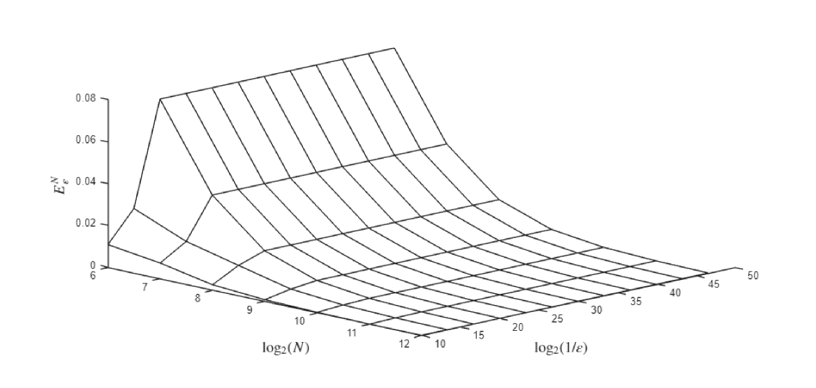
(a) On S–mesh

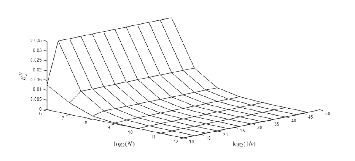
(b) On BS–mesh

Figure 1: Maximum pointwise errors $E_{\varepsilon}^{N}$ vs. $N$ and $\varepsilon$ for Example 1

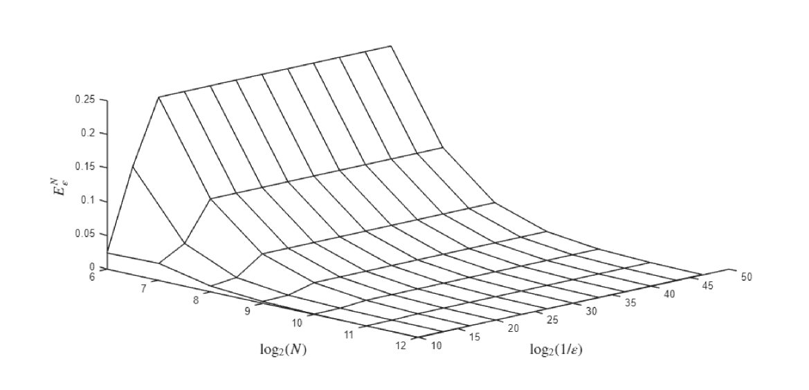
(c) On S–mesh

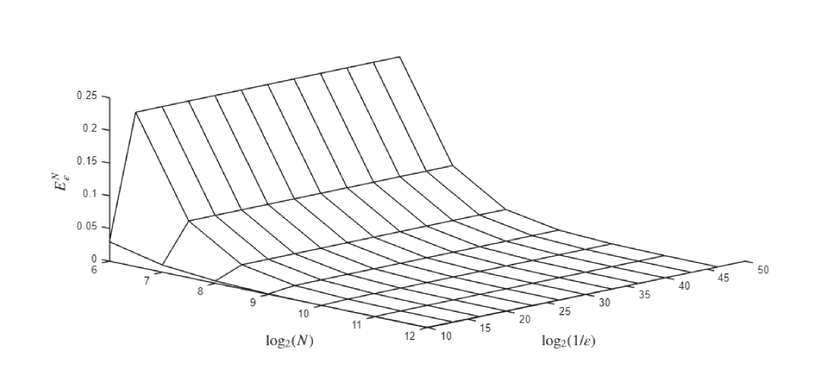
(d) On BS–mesh

Figure 2: Maximum pointwise errors $E_{\varepsilon}^{N}$ vs. $N$ and $\varepsilon$ for Example 2

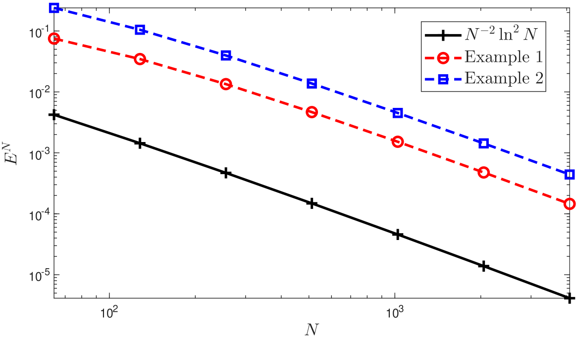
(a) On S-mesh

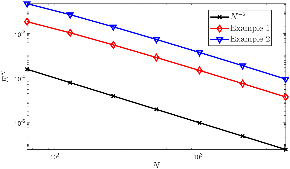
(b) On BS-mesh

Figure 3: Loglog plots of $E^{N}$ vs. $N$

Conclusion

In this work, we considered a weakly-coupled system of singularly perturbed problems of reaction-diffusion-type with Robin boundary conditions, where the leading terms are multiplied by small positive parameters that may vary in magnitude. The numerical solution was obtained using a piecewise-uniform Shishkin mesh and a modified Bakhvalov-Shishkin (BS) mesh. We carried out a detailed truncation error analysis and established the stability of the method. Theoretical results show that the scheme achieves exact second-order convergence on the BS mesh and nearly second-order convergence on the Shishkin mesh. To support these findings, two numerical experiments were conducted, confirming the parameter-uniform convergence of the method. The results clearly demonstrate that the proposed BS mesh yields more accurate solutions than the standard S-mesh for the same numerical scheme.

Data availability

No data was utilized for the research work done in this article.

CRediT authorship contribution statement

Kousalya Ramanujam: Conceptualization, Methodology, Software, Formal analysis, Investigation, Writing - original draft. Vembu Shanthi: Conceptualization, Methodology, Formal analysis, Investigation, Supervision, Writing - review & editing.

Declaration of competing interest

The authors have no competing interests to declare that are relevant to the content of this article.

References

- \bibcommenthead
- Miller et al. [2012] Miller, J.J.H., O’Riordan, E., Shishkin, G.I.: Fitted Numerical Methods for Singular Perturbation Problems: Error Estimates in the Maximum Norm for Linear Problems in One and Two Dimensions, Revised edn. World Scientific, Singapore (2012). https://doi.org/10.1142/2933
- Farrell et al. [2000] Farrell, P.A., Hegarty, A.F., Miller, J.J.H., O’Riordan, E., Shishkin, G.I.: Robust Computational Techniques for Boundary Layers. Applied Mathematics (Boca Raton), vol. 16, p. 254. Chapman & Hall/CRC, Boca Raton, FL (2000). https://doi.org/10.1201/9781482285727
- Roos et al. [2008] Roos, H.-G., Stynes, M., Tobiska, L.: Robust Numerical Methods for Singularly Perturbed Differential Equations: Convection-Diffusion-Reaction and Flow Problems. Springer Series in Computational Mathematics, vol. 24. Springer, Berlin (2008). https://doi.org/10.1007/978-3-540-34467-4
- Markowich [1984] Markowich, P.A.: A singular perturbation analysis of the fundamental semiconductor device equations. SIAM J. Appl. Math. 44(5), 896–928 (1984) https://doi.org/10.1137/0144064
- Markowich and Ringhofer [1984] Markowich, P.A., Ringhofer, C.A.: A singularly perturbed boundary value problem modelling a semiconductor device. SIAM J. Appl. Math. 44(2), 231–256 (1984) https://doi.org/10.1137/0144018
- Brezzi et al. [1986] Brezzi, F., Capelo, A., Marini, L.D.: Singular perturbation problems in semiconductor devices. In: Numerical Analysis (Guanajuato, 1984). Lecture Notes in Math., vol. 1230, pp. 191–198. Springer, Berlin (1986). https://doi.org/10.1007/BFb0072681
- Sreenivasan and Schumacher [2025] Sreenivasan, K.R., Schumacher, J.: What is the turbulence problem, and when may we regard it as solved? Annual Review of Condensed Matter Physics 16(1), 121–143 (2025) https://doi.org/10.1146/annurev-conmatphys-031620-095842
- Rodi [1993] Rodi, W.: Turbulence Models and Their Application in Hydraulics: a State-of-the-art Review, 3. ed edn. IAHR monograph series. Balkema, Rotterdam (1993). https://doi.org/10.1201/9780203734896
- Thomas [1998] Thomas, G.P.: Towards an improved turbulence model for wave-current interactions. Technical report, EU MAST-III Project (1998). The Kinematics and Dynamics of Wave-Current Interactions
- Hegarty et al. [1993] Hegarty, A.F., Miller, J.J.H., O’Riordan, E., Shishkin, G.I.: Key to the computation of the transfer of a substance by convection-diffusion in a laminar fluid. In: Applications of Advanced Computational Methods for Boundary and Interior Layers. Adv. Comput. Methods Bound. Inter. Layers, vol. 2, pp. 94–107. Boole, Dublin (1993)
- Naidu and Calise [2001] Naidu, D.S., Calise, A.J.: Singular perturbations and time scales in guidance and control of aerospace systems: A survey. Journal of Guidance, Control, and Dynamics 24(6), 1057–1078 (2001) https://doi.org/10.2514/2.4830
- Kazakov et al. [2006] Kazakov, A., Chaos, M., Zhao, Z., Dryer, F.L.: Computational singular perturbation analysis of two-stage ignition of large hydrocarbons. The Journal of Physical Chemistry A 110(21), 7003–7009 (2006) https://doi.org/10.1021/jp057224u
- Shafique et al. [2016] Shafique, Z., Mustafa, M., Mushtaq, A.: Boundary layer flow of maxwell fluid in rotating frame with binary chemical reaction and activation energy. Results in Physics 6, 627–633 (2016) https://doi.org/10.1016/j.rinp.2016.09.006
- Turner and LaBrake [2018] Turner, J., LaBrake, S.: Elementary Computational Fluid Dynamics Using Finite-Difference Methods. Union College Honors Thesis. Accessed: 2025-07-11 (2018)
- Lalrinhlua et al. [2025] Lalrinhlua, B., Saeed, A.M., Ganie, A.H., Tiwari, R., Das, S., Mofarreh, F., Singhal, A.: Study of vibrations in smart materials semiconductor under differential imperfect contact mechanism and nanoscale effect with electromechanical coupling effect. Acta Mechanica 236(4), 2383–2403 (2025) https://doi.org/10.1007/s00707-025-04279-9
- Kumar et al. [2024] Kumar, S., Ishwariya, R., Das, P.: Impact of mixed boundary conditions and nonsmooth data on layer-originated nonpremixed combustion problems: Higher-order convergence analysis. Studies in Applied Mathematics 153(4), 12763 (2024) https://doi.org/10.1111/sapm.12763
- Singh et al. [2021] Singh, M.K., Singh, G., Natesan, S.: A unified study on superconvergence analysis of Galerkin FEM for singularly perturbed systems of multiscale nature. J. Appl. Math. Comput. 66(1-2), 221–243 (2021) https://doi.org/10.1007/s12190-020-01434-4
- Ansari and Hegarty [2003] Ansari, A.R., Hegarty, A.F.: Numerical solution of a convection diffusion problem with Robin boundary conditions. J. Comput. Appl. Math. 156(1), 221–238 (2003) https://doi.org/10.1016/S0377-0427(02)00913-5
- Cai and Liu [2004] Cai, X., Liu, F.: Uniform convergence difference schemes for singularly perturbed mixed boundary problems. In: Proceedings of the International Conference on Boundary and Interior Layers—Computational and Asymptotic Methods (BAIL 2002), vol. 166, pp. 31–54 (2004). https://doi.org/10.1016/j.cam.2003.09.038
- Das and Natesan [2012] Das, P., Natesan, S.: Higher-order parameter uniform convergent schemes for Robin type reaction-diffusion problems using adaptively generated grid. Int. J. Comput. Methods 9(4), 1250052–27 (2012) https://doi.org/10.1142/S0219876212500521
- Avudai Selvi and Ramanujam [2017] Avudai Selvi, P., Ramanujam, N.: A parameter uniform difference scheme for singularly perturbed parabolic delay differential equation with Robin type boundary condition. Appl. Math. Comput. 296, 101–115 (2017) https://doi.org/10.1016/j.amc.2016.10.027
- Gupta et al. [2023] Gupta, A., Kaushik, A., Sharma, M.: A higher-order hybrid spline difference method on adaptive mesh for solving singularly perturbed parabolic reaction-diffusion problems with Robin-boundary conditions. Numer. Methods Partial Differential Equations 39(2), 1220–1250 (2023) https://doi.org/10.1002/num.22931
- Gelu and Duressa [2024] Gelu, F.W., Duressa, G.F.: Efficient hybridized numerical scheme for singularly perturbed parabolic reaction–diffusion equations with robin boundary conditions. Partial Differential Equations in Applied Mathematics 10, 100662 (2024) https://doi.org/10.1016/j.padiff.2024.100662
- Saini et al. [2024] Saini, S., Das, P., Kumar, S.: Parameter uniform higher order numerical treatment for singularly perturbed Robin type parabolic reaction diffusion multiple scale problems with large delay in time. Appl. Numer. Math. 196, 1–21 (2024) https://doi.org/10.1016/j.apnum.2023.10.003
- Matthews et al. [2000] Matthews, S., Miller, J.J.H., O?Riordan, E., Shishkin, G.I.: A parameter-robust numerical method for a system of singularly perturbed ordinary differential equations. In: Vulkov, L.G., Miller, J.J.H., Shishkin, G.I. (eds.) Analytical and Numerical Methods for Convection-Dominated and Singularly Perturbed Problems, pp. 219–224. Nova Science Publishers, New York (2000)
- Linßand Madden [2003] Linß, T., Madden, N.: An improved error estimate for a numerical method for a system of coupled singularly perturbed reaction-diffusion equations. vol. 3, pp. 417–423 (2003). https://doi.org/10.2478/cmam-2003-0027
- Kaushik et al. [2024] Kaushik, A., Gupta, A., Jain, S., Toprakseven, Sharma, M.: An adaptive mesh generation and higher-order difference approximation for the system of singularly perturbed reaction?diffusion problems. Partial Differential Equations in Applied Mathematics 11, 100750 (2024) https://doi.org/10.1016/j.padiff.2024.100750
- Matthews et al. [2002] Matthews, S., O’Riordan, E., Shishkin, G.I.: A numerical method for a system of singularly perturbed reaction-diffusion equations. J. Comput. Appl. Math. 145(1), 151–166 (2002) https://doi.org/10.1016/S0377-0427(01)00541-6
- Madden and Stynes [2003] Madden, N., Stynes, M.: A uniformly convergent numerical method for a coupled system of two singularly perturbed linear reaction-diffusion problems. IMA J. Numer. Anal. 23(4), 627–644 (2003) https://doi.org/10.1093/imanum/23.4.627
- Linß and Madden [2009] Linß, T., Madden, N.: Layer-adapted meshes for a linear system of coupled singularly perturbed reaction–diffusion problems. IMA Journal of Numerical Analysis 29(1), 109–125 (2009) https://doi.org/10.1093/imanum/drm053