Probing the isolated vector magnetic field of structured laser beams by atoms

Abstract

Electric and magnetic fields are inherently coupled in an electromagnetic wave. However, structured light beams enable their spatial separation. In particular, azimuthally polarized laser beams exhibit a localized magnetic field on-axis without the electric counterpart. Recent study by Martín-Domene et al. [App. Phys. Lett. 124, 211101 (2024)] has shown that combining these beams enables the generation of locally isolated magnetic fields with a controllable direction and phase. In the present paper we propose a method to probe and characterize such magnetic fields by studying their interaction with a single trapped atom. In order to theoretically investigate magnetic sublevel populations and their dependence on the relative orientation and phase—i.e. the polarization state—of the isolated magnetic field, we use a time-dependent density-matrix method based on the Liouville–von Neumann equation. As illustrative cases, we consider the $2s^{2}2p^{2}\,{}^{3}P_{0}\,-\,2s^{2}2p^{2}\,{}^{3}P_{1}$, the $1s^{2}2s^{2}\,{}^{1}S_{0}\,-\,1s^{2}2s2p\,{}^{3}P_{2}$, and the $2s^{2}2p\;{}^{2}P_{1/2}\,-\,2s^{2}2p\;{}^{2}P_{3/2}$ transitions in ⁴⁰Ca¹⁴⁺, ¹⁰Be, and ³⁸Ar¹³⁺, respectively. Our results indicate that monitoring atomic populations serves as an effective tool for probing isolated vector magnetic fields, which opens avenues for studying laser-induced processes in atomic systems where electric field suppression is critical.

I Introduction

Structured light is an emerging cutting-edge field that refers to the ability to shape different degrees of freedom of an electromagnetic wave such as the amplitude, phase, and polarization state [1, 2, 3, 4, 5]. This field was boosted by the discovery that light beams with helical wave fronts, known as twisted modes, possess a finite projection of the orbital angular momentum (OAM) [6, 7, 8], which has found many applications in optics, nanophotonics, and atomic physics [9, 10, 11, 12].

Besides twisted modes, more complex field distributions can also be achieved. In particular, combinations of beams where the OAM and spin angular momentum (SAM) are antiparallel to each other give rise to vector beams (VB), characterized by their spatial dependent polarization state [13]. Remarkably, in order to accomplish the Maxwell equations, VB present nonzero longitudinal components on-axis [14, 15, 16], leading to distinct light-matter interactions [17, 18, 19, 20, 21, 22].

A noteworthy example of VB are the so-called azimuthally polarized beams. Such beams possess an azimuthal electric-field polarization pattern with a singularity on the vortex line, i.e. at the location of a longitudinal magnetic field [23]. Particular interest has been given to the enhancement of this isolated longitudinal magnetic field. Examples include the use of metallic nanoantennas [24, 25], photoionization in gases [26], or plasmonic nanostructures [27, 28]. Once being enhanced, the range of applications that rely only on interactions with the locally isolated magnetic field is wide within different research fields such as magnetic spectroscopy [29, 30], force microscopy [31], optical spectroscopy [32], ultrafast nonlinear magnetization dynamics in ferromagnets [33], and chiral media [34, 35].

A recent work proposed to superpose multiple azimuthally polarized VB propagating in different directions in order to generate locally isolated magnetic fields with a controllable direction and phase, i.e. isolated optical magnetic fields with controllable polarization state [36]. Up to the present, however, no experimental scheme exists to determine the orientation of such an isolated magnetic field, which we refer to as “magnetic light” in line with the term widely used in the fields of nanophotonics and plasmonics [37]. In the present work, we propose a method to characterize the magnetic-light orientation by studying its interaction with a single atom. Our approach relies on the analysis of population dynamics of ground-state magnetic sublevels. We demonstrate that population distribution strongly depends on the polarization state of “magnetic light”, and hence can be used to characterize this polarization.

This paper is organized as follows. In Sec. II we briefly recall the basic formulas needed to describe “magnetic light” as superpositions of azimuthally polarized VB. Moreover, the interaction of this light with an atom is treated by introducing Rabi frequency and density-matrix formalism based on the Liouville–von Neumann equation. Calculations for such Rabi frequencies have been performed for the $2s^{2}2p^{2}\,{}^{3}P_{0}\,-\,2s^{2}2p^{2}\,{}^{3}P_{1}$ magnetic dipole ($M1$) transition in Ca¹⁴⁺ in Sec. III.1 and the $1s^{2}2s^{2}\,{}^{1}S_{0}\,-\,1s^{2}2s2p\,{}^{3}P_{2}$ magnetic quadrupole ($M2$) transition in Be in Sec. III.2. Based on these calculations we found that atomic transitions induced by the “magnetic light” exhibit different selection rules than those known from photoexcitation by plane-waves. Detailed analysis of time-dependent atomic population dynamics is presented in Sec. III.3 for the $2s^{2}2p\,{}^{2}P_{1/2}\,-\,2s^{2}2p\,{}^{2}P_{3/2}$ transition in Ar¹³⁺. Our findings indicate that the orientation of the isolated magnetic field strongly affects magnetic sublevel populations. Finally, a summary of our results and an outlook are given in Sec. IV.

II Theory

II.1 Structured light modes

In this work, we investigate the coupling of a target atom to an isolated optical magnetic field. Below, we will show that this “magnetic light” can be constructed from a superposition of azimuthally polarized VB. The basic properties of such beams will be briefly recalled in Sec. II.1.1, while their superposition will be discussed in Sec. II.1.2.

II.1.1 Azimuthally polarized light beams

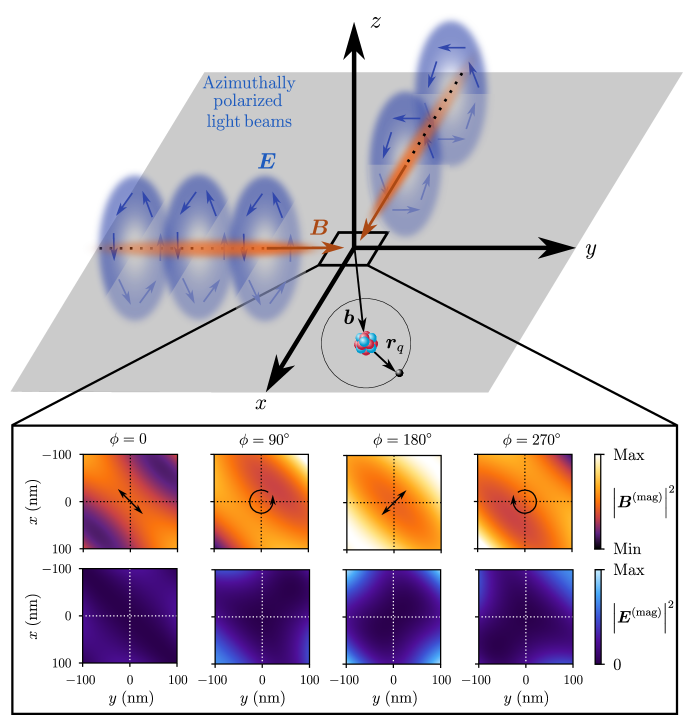
Figure 1: Geometry for the excitation of a single atom by a superposition of two azimuthally polarized VB, which propagate in the laboratory frame $x$ and $y$ direction, respectively. The intersection point of the beam axes is chosen as the origin of the coordinate system. The position of a target atom with respect to the origin is characterized by the impact parameter $\bm{b}$. The quantization $(z)$ axis is perpendicular to the propagation directions of both beams. The bottom inset shows the squared magnetic (top row) and electric (bottom row) fields given by Eqs. (21) and (22) for weights $c_{1}=c_{2}=1/\sqrt{2}$, opening angle $\theta_{k}=0.54^{\circ}$, and photon energy $\hbar\omega=2.73$ eV corresponding to a wavelength of $455$ nm. The arrows indicate the polarization of the magnetic field at the origin.

Azimuthally polarized light beams are typically described in terms of Laguerre-Gaussian or Hermite-Gaussian modes with different polarization states. In this work, we choose to construct the azimuthally polarized beam in the basis of the well-known Bessel states [38], as it allows a simpler treatment of structured-light matter interaction. These states are characterized by the longitudinal linear momentum $k_{z}$, the absolute value of the transverse momentum $|\bm{k}_{\perp}|=\varkappa$, the frequency $\omega=c\sqrt{k_{z}^{2}+\varkappa^{2}}=ck$, the helicity $\lambda$, and the well-defined projection $m_{\gamma}$ of the total angular momentum onto the propagation direction. The vector potential of Bessel radiation can be written in cylindrical coordinates ($r_{\perp}^{\prime},\phi_{r}^{\prime},z^{\prime}$) in the form

$$\begin{split}\bm{A}^{\mathrm{(B)}}_{m_{\gamma},\lambda}(\bm{r}^{\prime},t)=&\,A_{0}\sum\limits_{m_{s}=0,\pm 1}\bm{e}_{m_{s}}(-i)^{m_{s}}c_{m_{s}}J_{m_{\gamma}-m_{s}}(\varkappa r_{\perp}^{\prime})\\ &\times\mathrm{exp}[i(m_{\gamma}-m_{s})\phi_{r}^{\prime}+ik_{z}z^{\prime}-i\omega t],\end{split}$$ (1)

where the prime indicates that the $z^{\prime}$ axis, chosen along the light propagation direction, does not necessarily coincide with the quantization $z$ axis of the overall system. In Eq. (1), $A_{0}$ denotes the field amplitude, $J_{m_{\gamma}-m_{s}}(\varkappa r_{\perp}^{\prime})$ is the Bessel function of the first kind, and $\bm{e}_{\pm 1}=(\bm{e}_{x^{\prime}}\pm i\bm{e}_{y^{\prime}})/\sqrt{2}$ and $\bm{e}_{0}=\bm{e}_{z^{\prime}}$ are the polarization vectors. Moreover, the coefficients $c_{m_{s}}$ read as $c_{\pm 1}=\pm\lambda(1\pm\lambda\cos\theta_{k})/2$ and $c_{0}=-\sin\theta_{k}/\sqrt{2}$, where $\theta_{k}=\mathrm{arctan}(\varkappa/k_{z})$ is the polar opening angle [39, 40].

An azimuthally polarized VB can be written as a linear combination of two Bessel beams with $\lambda=\pm 1$ and $m_{\gamma}=0$:

$$\begin{split}\bm{A}^{\mathrm{(az)}}(\bm{r}^{\prime},t)=\frac{1}{\sqrt{2}}\Bigl[&\bm{A}^{\mathrm{(B)}}_{m_{\gamma}=0,\lambda=-1}(\bm{r}^{\prime},t)\\ &-\bm{A}^{\mathrm{(B)}}_{m_{\gamma}=0,\lambda=+1}(\bm{r}^{\prime},t)\Bigr].\end{split}$$ (2)

See Ref. [41] for more information. To better understand the properties of $\bm{A}^{\mathrm{(az)}}$, we expand it in multipoles:

$$\bm{A}^{\mathrm{(az)}}(\bm{r}^{\prime})=\sqrt{4\pi}\sum_{L}i^{L}\sqrt{2L+1}\;d^{L}_{0,-1}(\theta_{k})\;\bm{a}^{(0)}_{L0}(\bm{r}^{\prime}),$$ (3)

where $d^{L}_{0,1}$ are elements of the small Wigner $d$-matrix [42]. The complete absence of electric multipoles $\bm{a}^{(1)}_{L0}$ in Eq. (3) means that the target atom placed on the beam axis “sees” only magnetic multipoles $\bm{a}^{(0)}_{L0}$ of rank $L$. However, when the atom is displaced from the beam axis, both magnetic and electric multipoles contribute to the light-atom interaction.

Let us now calculate electric and magnetic fields of the azimuthally polarized VB. By using the standard relations $\bm{E}=-\partial_{t}\bm{A}$ and $\bm{B}=\nabla\times\bm{A}$, we obtain:

$$\bm{E}^{\mathrm{(az)}}(\bm{r}^{\prime},t)= \,i\omega A_{0}J_{1}(\varkappa r_{\perp}^{\prime})\mathrm{exp}[i(k_{z}z^{\prime}-\omega t)]\bm{e}_{\phi_{r}^{\prime}},$$ (4a)

$$\bm{B}^{\mathrm{(az)}}(\bm{r}^{\prime},t)= -ikA_{0}\cos\theta_{k}J_{1}(\varkappa r_{\perp}^{\prime})\mathrm{exp}[i(k_{z}z^{\prime}-\omega t)]\bm{e}_{r_{\perp}^{\prime}}$$

$$+kA_{0}\sin\theta_{k}J_{0}(\varkappa r_{\perp}^{\prime})\mathrm{exp}[i(k_{z}z^{\prime}-\omega t)]\bm{e}_{z^{\prime}},$$ (4b)

where $\bm{e}_{r_{\perp}^{\prime}}$, $\bm{e}_{\phi_{r}^{\prime}}$ and $\bm{e}_{z^{\prime}}$ are the basis unit vectors. From Eq. (4a), we see that the electric field vector is directed along the azimuthal direction $\bm{e}_{\phi_{r}^{\prime}}$, thus justifying the name azimuthally polarized beam. For the present work, it is important to note that the electric field $\bm{E}^{\mathrm{(az)}}$ vanishes on the beam axis, $r_{\perp}^{\prime}=0$, while the longitudinal component of the magnetic field is nonzero:

$$\bm{E}^{\mathrm{(az)}}(r_{\perp}^{\prime}=0,z^{\prime},t)= \,0,$$ (5a)

$$\bm{B}^{\mathrm{(az)}}(r_{\perp}^{\prime}=0,z^{\prime},t)= \,kA_{0}\sin\theta_{k}\mathrm{exp}[i(k_{z}z^{\prime}-\omega t)]\bm{e}_{z^{\prime}},$$ (5b)

as discussed in Ref. [17].

II.1.2 Magnetic light

At the beam center, $r_{\perp}^{\prime}=0$, an azimuthally polarized VB (5) exhibits a longitudinal magnetic field along the beam axis, $\bm{B}^{\mathrm{(az)}}\parallel\bm{e}_{z^{\prime}}$. By applying a second azimuthally polarized beam, one can rotate $\bm{B}$ in arbitrary direction [36]. In Fig. 1, for example, we consider a geometry where two azimuthally polarized VB propagate perpendicular to each other along the $x$ and $y$ axes. In this chosen geometry the quantization $(z)$ axis is directed perpendicular to the axes of both beams. The reference frame defined in this way will be referred to as the laboratory frame with the origin at the intersection of both beam axes.

For the geometry displayed in Fig. 1, the vector potential of a superposition of two azimuthally polarized VB takes the form

$$\bm{A}^{\mathrm{(mag)}}(\bm{r},t)=c_{\mathrm{1}}\bm{A}^{\mathrm{(az)}}_{x}(\bm{r},t)+c_{\mathrm{2}}\,\mathrm{exp}[i\phi]\bm{A}^{\mathrm{(az)}}_{y}(\bm{r},t).$$ (6)

Here the real weights satisfy $c_{\mathrm{1}}^{2}+c_{\mathrm{2}}^{2}=1$, and $\phi$ is the relative phase between the components. It should be noted that in Eq. (6) both vector potentials $\bm{A}^{\mathrm{(az)}}_{x}$ and $\bm{A}^{\mathrm{(az)}}_{y}$ are given in the laboratory frame, whereas in Sec. II.1.1 they are written in the local frame with the $z^{\prime}$ axis along the light propagation direction. The transformation from one reference frame to another can be readily done and the details are omitted.

Similar to Eq. (3), we expand the light field in Eq. (6) in multipoles:

$$\begin{split}\bm{A}^{\mathrm{(mag)}}(\bm{r})=&\sqrt{4\pi}\sum_{LM}i^{L}\sqrt{2L+1}\;d^{L}_{0,-1}(\theta_{k})\;d^{L}_{M,0}(\pi/2)\\ &\times\;\bm{a}^{(0)}_{LM}(\bm{r})\Bigl(c_{1}+c_{2}\,\mathrm{exp}[i(\phi-M\,\pi/2)]\Bigr).\end{split}$$ (7)

A conclusion from Eq. (7) is that an atom placed at the origin, $\bm{r}=0$, can interact only with magnetic multipoles. For this reason, we will refer to the field described by Eq. (6) as “magnetic light”. As we have already mentioned, the exclusion of electric multipoles from the coupling between light and matter depends on the position of the atom, but not on its size. Thus the concept of “magnetic light” is determined not only by the properties of the light itself, but also by the position of the observer (atom).

By making use of the vector potential (6), one can obtain the electric and magnetic fields of the superposed beams. The expressions for these fields are given in Appendix A for arbitrary $\bm{r}$, and their time-averaged spatial distributions, $\left|\bm{E}^{\mathrm{(mag)}}\right|^{2}$ and $\left|\bm{B}^{\mathrm{(mag)}}\right|^{2}$, are presented in the bottom inset of Fig. 1 for different phases $\phi$. As seen from this figure, “magnetic light”, contrary to its name, exhibits not only a magnetic, but also an electric field. This is not surprising, because magnetic multipoles of the radiation field consist of both magnetic and electric fields [42, 43]. But despite the presence of the electric field, “magnetic light” can only excite magnetic multipole transitions if an atom is located at $\bm{r}=0$. As we will see below, the excitation process reflects the symmetry of “magnetic light” at the origin. The electric and magnetic fields at this point are:

$$\bm{E}^{\mathrm{(mag)}}(\bm{r}=0,t)= \,0,$$ (8a)

$$\bm{B}^{\mathrm{(mag)}}(\bm{r}=0,t)= \,kA_{0}\sin\theta_{k}\mathrm{exp}[-i\omega t]$$

$$\times\Bigl(c_{1}\bm{e}_{x}+c_{2}\mathrm{exp}[i\phi]\bm{e}_{y}\Bigr).$$ (8b)

As seen from these expressions, the electric field $\bm{E}^{\mathrm{(mag)}}$ vanishes at $\bm{r}=0$, in contrast to the nonzero magnetic field $\bm{B}^{\mathrm{(mag)}}$, which is directed perpendicular to the quantization axis. Such a magnetic field oscillates at optical frequency and its “polarization” is determined by the phase $\phi$ and the coefficients $c_{1}$ and $c_{2}$. It should be recalled that polarization usually refers to the orientation of the electric field of an electromagnetic wave. Since $\bm{E}^{\mathrm{(mag)}}(\bm{r}=0)=0$, we will exploit this term to specify the direction of the magnetic field at the origin. In the case when $c_{1}=c_{2}=1/\sqrt{2}$, the phase $\phi=0^{\circ}$ or $180^{\circ}$ leads to linear polarization, while $\phi=90^{\circ}$ or $270^{\circ}$ corresponds to circular polarization. See Ref. [36] for more details.

II.2 Rabi frequency

II.2.1 Plane-wave radiation

We continue our theoretical analysis with a brief reminder of the excitation of an atom by plane-wave radiation. In particular, we consider a transition between ground $\left|\alpha_{g}F_{g}M_{g}\right>$ and excited $\left|\alpha_{e}F_{e}M_{e}\right>$ atomic states with the total angular momentum $\bm{F}=\bm{I}+\bm{J}$, where $\bm{I}$ and $\bm{J}$ are the nuclear and electron angular momenta, respectively, $M$ is the projection of $\bm{F}$ onto the $z$ axis, and $\alpha$ refers to all additional quantum numbers. In atomic physics, it is natural to characterize the coupling between these two states by the Rabi frequency

$$\begin{split}\Omega_{R}^{\mathrm{(pl)}}=&\,\Biggl|\frac{A_{0}ec}{\hbar}\Biggl<\alpha_{e}F_{e}M_{e}\bigg|\sum\limits_{q}\bm{\alpha}_{q}\cdot\bm{e}^{\mathrm{(pl)}}e^{i\bm{k}\cdot\bm{r}_{q}}\bigg|\alpha_{g}F_{g}M_{g}\Biggr>\Biggr|\\ =&\;\widetilde{\Omega}_{R}\biggl|\frac{i^{p}}{\sqrt{2}}\left<F_{g}\,M_{g}\,L\,1|F_{e}\,M_{e}\right>(ic_{1}+c_{2}\mathrm{exp}[i\phi])\\ &\;-\frac{(-i)^{p}}{\sqrt{2}}\left<F_{g}\,M_{g}\,L\,-1|F_{e}\,M_{e}\right>(ic_{1}-c_{2}\mathrm{exp}[i\phi])\biggr|,\end{split}$$ (9)

where we have introduced the so-called reduced frequency

$$\begin{split}\widetilde{\Omega}_{R}=&\,\biggl|\frac{A_{0}ec}{\hbar}\sqrt{2\pi(2L+1)(2F_{g}+1)}\begin{Bmatrix}F_{e}&F_{g}&L\\ J_{g}&J_{e}&I\end{Bmatrix}\\ &\times\left<\alpha_{e}J_{e}||H_{\gamma}(pL)||\alpha_{g}J_{g}\right>\biggr|,\end{split}$$ (10)

and $\left<\alpha_{e}J_{e}||H_{\gamma}(pL)||\alpha_{g}J_{g}\right>$ denotes the reduced matrix element for the magnetic ($p=0$) or electric ($p=1$) transition of the order $L$ [44]. Moreover, $\bm{r}_{q}$ determines the position of the $q$th electron with respect to the atomic center of mass, and $\bm{\alpha}_{q}$ denotes the vector of Dirac matrices [45, 46]. When deriving Eq. (9), we have assumed that the transition proceeds via only one multipole channel and that the plane wave propagates along the $z$ axis and has polarization $\bm{e}^{\mathrm{(pl)}}=c_{2}\,\mathrm{exp}[i\phi]\bm{e}_{x}-c_{1}\bm{e}_{y}$. Such a parametrization ensures that the direction of the magnetic field of the plane wave coincides with the local magnetic field of the “magnetic light” at $\bm{r}=0$, see Eq. (8b).

The Rabi frequency (9) is nonzero if the angular-momentum and parity selection rules

$$|F_{e}-F_{g}|\leq \ L\leq F_{e}+F_{g},$$ (11a)

$$M_{e}-M_{g}= \ \Delta M=\pm 1,$$ (11b)

$$\pi_{g}\pi_{e}= \ (-1)^{L+p+1},$$ (11c)

are satisfied. Here, $\pi_{g}$ and $\pi_{e}$ are the parities of the ground and excited states, respectively [42].

II.2.2 Magnetic light

Having examined the interaction with plane-wave radiation, we move on to a discussion of the coupling between a target atom and the “magnetic light”. Let us, for the moment, assume that the center of mass of the atom is located at the origin, $\bm{r}=0$. As discussed above, at this position only magnetic multipoles contribute to the excitation, see Eq. (7).

It can be shown after some angular momentum algebra that the Rabi frequency for the transition between the $\left|\alpha_{g}F_{g}M_{g}\right>$ and $\left|\alpha_{e}F_{e}M_{e}\right>$ states induced by the “magnetic light” (6) is given by

$$\begin{split}\Omega_{R}^{\mathrm{(mag)}}=&\,\left|\frac{ec}{\hbar}\left<\alpha_{e}F_{e}M_{e}\bigg|\sum\limits_{q}\bm{\alpha}_{q}\cdot\bm{A}^{\mathrm{(mag)}}(\bm{r}_{q})\bigg|\alpha_{g}F_{g}M_{g}\right>\right|\\ =&\;\widetilde{\Omega}_{R}\Bigl|\left<F_{g}\,M_{g}\,L\,\Delta M|F_{e}\,M_{e}\right>\\ &\qquad\times\sqrt{2}\;\delta_{0,p}\;d^{L}_{0,1}(\theta_{k})\;d^{L}_{\Delta M,0}(\pi/2)\\ &\qquad\times\Bigl(c_{1}+c_{2}\,\mathrm{exp}[i(\phi-\Delta M\,\pi/2)]\Bigr)\Bigr|,\end{split}$$ (12)

From Eq. (12) we deduce the selection rules

$$|F_{e}-F_{g}|\leq \;L\leq F_{e}+F_{g},$$ (13a)

$$M_{e}-M_{g}=\Delta M= \,-L,-L+2,\dots,L-2,L,$$ (13b)

$$p=0\;\;\mathrm{and} \;\;\pi_{g}\pi_{e}=\ (-1)^{L+1}.$$ (13c)

Note that the $\Delta M$ selection rule (13b) is in general different from that for plane waves (11b). Indeed, the difference of angular momentum projection $\Delta M$ changes in steps of two. This angular-momentum selection rule is related to the fact that $d^{L}_{\Delta M,0}(\pi/2)\propto\delta_{L-\Delta M,2n}$, where $n$ is an integer [47]. There is one unique case where Eqs. (13) coincide with the plane-wave selection rules given by Eqs. (11). This is the $M1$ transition for which $F_{e}-F_{g}=0,\pm 1$, $\Delta M=\pm 1$, and $\pi_{g}\pi_{e}=1$. In the case of non-dipole transitions, Eqs. (13) predict a different selection rule for $\Delta M$. In particular, for an $M2$ transition we have $\Delta M=0,\pm 2$, in contrast to $\Delta M=\pm 1$ for the plane-wave case.

II.3 Density matrix formalism

The Rabi frequency provides general information about the strength of the coupling between a target atom and the incident radiation. In the absence of relaxation, this frequency uniquely determines the time dependence of populations of atomic states. In order to investigate the time evolution of the system in the presence of relaxation, a more detailed analysis based on the density matrix theory is required [48, 49]. In this approach, the state of the system is represented by the density operator $\hat{\rho}(t)$ that satisfies the Liouville–von Neumann equation:

$$\frac{\mathrm{d}}{\mathrm{d}t}\hat{\rho}(t)=-\frac{i}{\hbar}\left[\hat{H}(t),\hat{\rho}(t)\right]+\hat{R}(t).$$ (14)

Here, $\hat{H}(t)$ is the total Hamiltonian of an atom in the presence of both the incident radiation and an external magnetic field. Moreover, the operator $\hat{R}(t)$ has been added “by hand” to account for relaxation due to radiative decay [50].

For further analysis, it is more convenient to rewrite Eq. (14) in matrix form. For this purpose, we choose a set of basis states $\left|\alpha FM\right>$. The resulting system of coupled differential equations for the density-matrix elements can be found in Refs. [51, 52]. We then solve these equations to find the density matrix as a function of time.

In order to visualize the results and simplify the discussion, it is practical to describe the population of atomic states in terms of the so-called statistical tensors

$$\begin{split}\rho_{kq}(\alpha F;t)=&\,\sum\limits_{M\,M^{\prime}}(-1)^{F-M^{\prime}}\left<F\,M\,F\,-M^{\prime}|k\,q\right>\\ &\times\left<\alpha FM|\hat{\rho}(t)|\alpha FM^{\prime}\right>,\end{split}$$ (15)

which transform like spherical harmonics of rank $k$ under a rotation of the coordinates [53]. The normalization of $\rho_{kq}$ by means of the zero-rank tensor

$$\mathcal{A}_{kq}(\alpha F;t)=\frac{\rho_{kq}(\alpha F;t)}{\rho_{00}(\alpha F;t)}$$ (16)

gives rise to the orientation ($k$ odd) and alignment ($k$ even) parameters. These parameters describe the relative population of atomic sublevels $\left|\alpha FM\right>$ and coherence between them.

III Results and Discussion

Equations (9)-(16) can be applied to any atom or ion, independent of its nuclear spin and electronic shell structure. Below, we consider three systems: (i) the $2s^{2}2p^{2}\;{}^{3}P_{0}\,-\,2s^{2}2p^{2}\;{}^{3}P_{1}$ transition in ⁴⁰Ca¹⁴⁺, (ii) the $1s^{2}2s^{2}\;{}^{1}S_{0}\,-\,1s^{2}2s2p\;{}^{3}P_{2}$ transition in ¹⁰Be, and (iii) the $2s^{2}2p\;{}^{2}P_{1/2}-2s^{2}2p\;{}^{2}P_{3/2}$ transition in ³⁸Ar¹³⁺. In all cases, the nuclear spin is $I=0$, so that we are dealing with transitions between fine-structure levels. The atoms are placed directly at the intersection point of both beam axes. The VB are tuned to exact resonance with the transition. It is assumed that $c_{1}=c_{2}=1/\sqrt{2}$. Such weights lead to linear polarization of light when $\phi=0^{\circ}$ or $180^{\circ}$ and circular polarization when $\phi=90^{\circ}$ or $270^{\circ}$. Moreover, we have chosen the parameters $A_{0}$ and $\theta_{k}$ such that in the vicinity of the beam center the vector potential (1) reproduces an experimentally realistic Laguerre-Gaussian mode with a waist equal to $44$ wavelengths and a total power of 1 $\mu$W. With these conditions, the isolated magnetic field strength is of the order of $10^{-8}$ T.

III.1 ${}^{\textbf{3}}$P${}_{\textbf{0}}\rightarrow{}^{\textbf{3}}$P${}_{\textbf{1}}$ transition in Ca¹⁴⁺

We start with the ${}^{3}P_{0}-{}^{3}P_{1}$ $M1$ transition in ⁴⁰Ca¹⁴⁺ ion. The relatively long lifetime of the excited state of about $10.5$ ms [54] allows us to neglect spontaneous decay for interaction times shorter than 1 ms. At such time intervals, the entire evolution of the system is simply Rabi oscillations at the frequencies $\Omega_{R}$. Fig. 2 shows graphs of $\Omega_{R}$ divided by the reduced frequency (10). The latter is equal to $\widetilde{\Omega}_{R}=2\pi\times 215$ kHz for the chosen set of parameters. The results for plane waves (dashed lines) and “magnetic light” (solid lines) are presented as a function of the relative phase $\phi$, which determines the polarization. As seen from Fig. 2, the Rabi frequencies for both light fields show qualitatively the same behavior. Namely, only the $M_{e}=\pm 1$ magnetic sublevels are excited, as follows from the selection rules (11) and (13), and $\Omega_{R}^{\mathrm{(mag)}}$ has exactly the same phase dependence as $\Omega_{R}^{\mathrm{(pl)}}$. In particular, for $\phi=0^{\circ}$ the magnetic field of both types of radiation has linear polarization, leading to $\Omega_{R}(M_{e}=+1)=\Omega_{R}(M_{e}=-1)$. In contrast, $\Omega_{R}(M_{e}=+1)\neq 0$ and $\Omega_{R}(M_{e}=-1)=0$ for $\phi=90^{\circ}$, which corresponds to magnetic field with circular polarization.

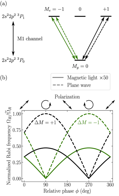
Figure 2: (a) The $2s^{2}2p^{2}\,{}^{3}P_{0}\,-\,2s^{2}2p^{2}\,{}^{3}P_{1}$ magnetic dipole transition in ⁴⁰Ca¹⁴⁺. The arrows indicate the interaction with “magnetic light” (solid) and plane waves (dashed). Shown are $M_{g}=0\rightarrow M_{e}=+1$ (black) and $M_{g}=0\rightarrow M_{e}=-1$ (green) transitions. The atom is located at the origin of the coordinate system. (b) Normalized Rabi frequencies for these transitions as a function of the relative phase $\phi$ which determines the light polarization (top). Here, the weights are $c_{1}=c_{2}=1/\sqrt{2}$, the photon energy is $\hbar\omega=2.18$ eV, and the polar opening angle is $\theta_{k}=0.54^{\circ}$.The values for “magnetic light” are increased by a factor of 50.

III.2 ${}^{\textbf{1}}$S${}_{\textbf{0}}\rightarrow{}^{\textbf{3}}$P${}_{\textbf{2}}$ transition in Be

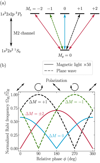
Figure 3: (a) The $1s^{2}2s^{2}\,{}^{1}S_{0}\,-\,1s^{2}2s2p\,{}^{3}P_{2}$ magnetic quadrupole transition in ¹⁰Be. “Magnetic light” induces $M_{g}=0\rightarrow M_{e}=\pm 2$ (red solid line) and $M_{g}=0\rightarrow M_{e}=0$ (blue solid line) transitions. Plane waves induce $M_{g}=0\rightarrow M_{e}=+1$ (black dashed line) and $M_{g}=0\rightarrow M_{e}=-1$ (green dashed line) transitions. (b) Phase dependence of normalized Rabi frequencies. The photon energy is $\hbar\omega=2.73$ eV. All other parameters are the same as in Fig. 2.

In contrast to the ${}^{3}P_{0}-{}^{3}P_{1}$ $M1$ case described above, the ${}^{1}S_{0}-{}^{3}P_{2}$ transition in ¹⁰Be proceeds via the $M2$ channel. Since the multipole is higher, the transition is weaker. As a consequence, the lifetime of the excited state increases to 6061 s [55] and the reduced frequency decreases to $\widetilde{\Omega}_{R}=2\pi\times 327$ Hz. Fig. 3 shows the transition scheme and the normalized Rabi frequencies $\Omega_{R}^{\mathrm{(pl)}}/\widetilde{\Omega}_{R}$ and $\Omega_{R}^{\mathrm{(mag)}}/\widetilde{\Omega}_{R}$ as a function of $\phi$. It can be seen that plane waves and “magnetic light” drive different transitions. The plane wave only couples the $M_{g}=0$ ground state to the $M_{e}=\pm 1$ excited state, while the “magnetic light” drives transitions $\left|M_{g}=0\right>\rightarrow\left|M_{e}=0,\pm 2\right>$. Such behavior follows the selection rules given by Eqs. (11) and (13), as discussed above.

In addition to different $\Delta M$ selection rules, Fig. 3 also shows qualitatively different dependence of $\Omega_{R}^{\mathrm{(pl)}}$ and $\Omega_{R}^{\mathrm{(mag)}}$ on the phase $\phi$, and hence polarization. For example, for $\phi=90^{\circ}$ and $270^{\circ}$ both plane waves and “magnetic light” exhibit right and left circular polarization. For the plane-wave case this circular polarization can be attributed to helicity $\pm 1$ which results in transition between sublevels with $\Delta M=\pm 1$. The predictions for the “magnetic light” look counterintuitive: despite of circular polarization, one can induce $\Delta M=0,\pm 2$ transitions. This behavior can be understood from the conservation of total angular momentum projection on the quantization axis. Indeed, by analyzing the expectation value of the $z$-component of the total angular momentum operator $\left<\hat{J}_{z}\right>$, one obtains the well-know result $\left<\hat{J}_{z}\right>=\hbar\lambda$ for plane waves with circular polarization. In contrast, $\left<\hat{J}_{z}\right>=0$ for $L=2$ multipoles of circularly polarized “magnetic light”. Together with the selection rules (13), this implies that only excitation to the sublevels $M_{e}=0,\pm 2$ is possible. For the latter case, the substates $\left|M_{e}=\pm 2\right>$ must be equally populated, so that $\left<\hat{J}_{z}^{\mathrm{(atom)}}\right>=0$.

In the case when $\phi=0^{\circ}$ and $180^{\circ}$ plane waves and magnetic-light radiation are linearly polarized. For plane waves, both orientations of linear polarization result in equal population of $M_{e}=\pm 1$ substates, i.e. $\Omega_{R}^{\mathrm{(pl)}}(M_{e}=+1)=\Omega_{R}^{\mathrm{(pl)}}(M_{e}=-1)$. In contrast, “magnetic light” with opposite directions of linear polarization leads to different coupling of atomic sublevels. While, for example, $\Omega_{R}^{\mathrm{(mag)}}(M_{e}=0)\neq 0$ for $\phi=0^{\circ}$, it vanishes for $\phi=180^{\circ}$. To explain this behavior, we refer to Fig. 1 which indicates that rotation of the polarization vector of “magnetic light” by $90^{\circ}$ is connected to a change of electric and magnetic field distributions and hence the symmetry of the system.

III.3 ${}^{\textbf{2}}$P${}_{\textbf{1/2}}\rightarrow{}^{\textbf{2}}$P${}_{\textbf{3/2}}$ transition in Ar¹³⁺

In the previous sections, we discussed the Rabi frequency $\Omega_{R}$ for $M1$ and $M2$ transitions in ⁴⁰Ca¹⁴⁺ and ¹⁰Be atoms, respectively. In what follows, we consider time-dependent population dynamics for the ${}^{2}P_{1/2}\,-\,{}^{2}P_{3/2}$ transition in ³⁸Ar¹³⁺ including relaxation due to spontaneous emission, see Fig. 4 (a). This spontaneous emission can proceed via $M1$ and electric quadrupole $(E2)$ channels. However, the decay rate $\Gamma_{E2}$ is rather small compared to $\Gamma_{M1}$ [56], and hence $E2$ decay will be omitted. To investigate atomic population dynamics, we solve the Liouville-von Neumann equation (14).

III.3.1 Orientation parameter $\mathcal{A}_{10}$

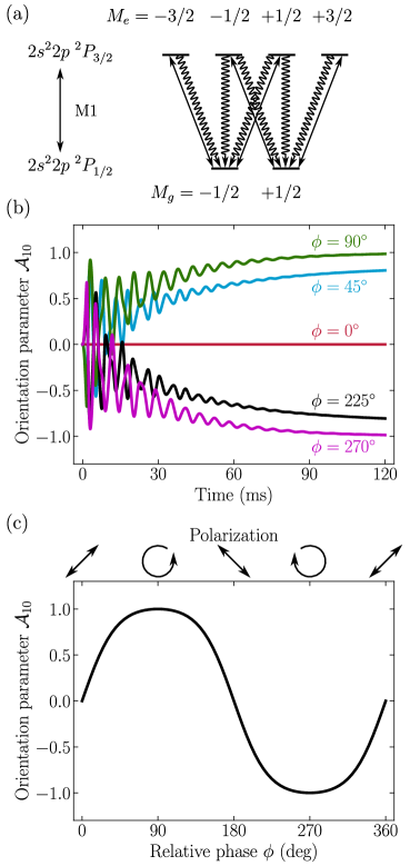
Figure 4: (a) The $2s^{2}2p\;{}^{2}P_{1/2}\,-\,2s^{2}2p\;{}^{2}P_{3/2}$ magnetic dipole transition in ³⁸Ar¹³⁺. The arrows represent the interactions with “magnetic light” (6), and the wavy lines represent spontaneous decay. (b) Time dependence of the orientation $\mathcal{A}_{10}$ of the $2s^{2}2p\;{}^{2}P_{1/2}$ ground state for different relative phases: $\phi=0^{\circ}$ (red), $\phi=45^{\circ}$ (blue), $\phi=90^{\circ}$ (green), $\phi=225^{\circ}$ (black), and $\phi=270^{\circ}$ (magenta). (c) Steady-state orientation $\mathcal{A}_{10}$ as a function of the relative phase $\phi$. The photon energy is $\hbar\omega=2.81$ eV. All other parameters are the same as in Fig. 2.

Below we will pay special attention to the relative population of the $\left|2s^{2}2p\;{}^{2}P_{1/2}\;M_{g}=\pm 1/2\right>$ magnetic sublevels. As discussed in Sec. II.3, it is convenient to describe this relative population in terms of the orientation parameter

$$\mathcal{A}_{10}(t)=\frac{\rho_{+1/2}(t)-\rho_{-1/2}(t)}{\rho_{+1/2}(t)+\rho_{-1/2}(t)},$$ (17)

with substate population

$$\rho_{M_{g}}(t)=\left<2s^{2}2p\,{}^{2}P_{1/2}\,M_{g}\right|\hat{\rho}(t)\left|2s^{2}2p\,{}^{2}P_{1/2}\,M_{g}\right>,$$ (18)

which follows from Eqs. (15) and (16). The time evolution of the ground-state orientation $\mathcal{A}_{10}$, produced in the course of the interaction with the “magnetic light”, is shown in Fig. 4 (b). It can be seen from the figure that the atomic sublevel population reaches steady state in hundreds of milliseconds after performing several Rabi oscillations. As described in Ref. [57], this behavior corresponds to light damping regime for which the ratio of the damping rate $\Gamma_{M1}=0.1$ kHz to the Rabi frequency $\Omega_{R}^{\mathrm{(mag)}}\approx 1$ kHz is of the order of $\Gamma_{M1}/\Omega_{R}^{\mathrm{(mag)}}\approx 0.1$. In the following, we focus on the analysis of the steady-state orientation parameter, i.e. $\mathcal{A}_{10}(t>120\penalty 10000\ \mathrm{ms})$.

The steady-state orientation $\mathcal{A}_{10}$ is shown in Fig. 4 (c) as a function of the relative phase $\phi$. From this figure and Eq. (17), one can see that ${}^{2}P_{1/2}$ ground state is fully oriented for $\phi=90^{\circ}$ and $270^{\circ}$ which corresponds to right and left circular polarization of “magnetic light”, respectively. This resembles the outcome of photoexcitation by circularly polarized plane waves and can be understood by analysis of conservation of total angular momentum projection. Indeed, $\left<\hat{J}_{z}\right>=\pm\hbar$ for “magnetic light” with $\phi=90^{\circ}$ and $270^{\circ}$ which results in pumping of the population into the magnetic substate $M_{g}=\pm 1/2$ after several Rabi cycles. In contrast, in the case when $\phi=0^{\circ}$ and $180^{\circ}$, the “magnetic light” is linearly polarized and carries $\left<\hat{J}_{z}\right>=0$, but this does not lead to atomic orientation. Such a zero atomic orientation is also well known from photoexcitation by plane waves with linear polarization. It follows from Fig. 4 (c) and our discussion that the orientation of the ${}^{2}P_{1/2}$ ground state can be used to study the magnetic-light polarization. This orientation can be measured, for example, by state dependent fluorescence [58, 59].

III.3.2 Beam-weight dependence of $\mathcal{A}_{10}$

Above we showed that the orientation $\mathcal{A}_{10}$ of the ${}^{2}P_{1/2}$ state of Ar¹³⁺ is very sensitive to the relative phase between magnetic-light components (6) with equal weights $c_{1}=c_{2}=1/\sqrt{2}$. In this scenario both azimuthally polarized VB have equal total power. However, the weights $c_{1}$ and $c_{2}$ may not always be equal in experiments. In order to account for such unequal beam weights and make the proposed diagnostic method even more accessible, we study here the atomic ground-state orientation for cases when $c_{1}\neq c_{2}$.

We note that when $c_{1}\neq c_{2}$ the phase $\phi$ still uniquely determines the handedness of the magnetic-light polarization. Together, $c_{1}$, $c_{2}$, and $\phi$ specify this polarization which might differ from that obtained in the case of equal weights. Indeed, as seen from Eq. (8b) the “magnetic light” is linearly polarized for all values of $c_{1}$ and $c_{2}$ when $\phi=0^{\circ}$ and $180^{\circ}$. For $\phi=90^{\circ}$ and $270^{\circ}$ as well as $c_{1}\neq c_{2}$, Eq. (8b) predicts “magnetic light” with elliptical polarization which approaches linear polarization when $c_{1}\gg c_{2}$ or $c_{1}\ll c_{2}$.

The orientation $\mathcal{A}_{10}$ for different weights $c_{1}$ and $c_{2}$ is displayed in Fig. 5 as a function of $\phi$. It is shown that the relative-phase sensitivity of the atomic orientation is maximal for $c_{1}=c_{2}$, i.e. when the “magnetic light” changes polarization state from linear to circular. This sensitivity becomes less pronounced in the limit $c_{1}\gg c_{2}$ as follows from analysis of $\left<\hat{J}_{z}\right>$. Indeed, we find $\left<\hat{J}_{z}\right>=0$ for all weights when $\phi=0^{\circ}$ and $180^{\circ}$, leading to vanishing $\mathcal{A}_{10}$. In contrast, $\Bigl|\left<\hat{J}_{z}(c_{1}=c_{2})\right>\Bigr|=\hbar>\Bigl|\left<\hat{J}_{z}(c_{1}\neq c_{2})\right>\Bigr|$ in the case when $\phi=90^{\circ}$ and $270^{\circ}$ which results in declining atomic orientation.

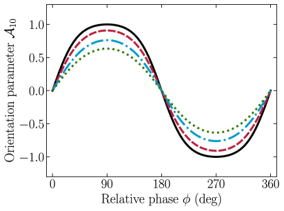
Figure 5: Same as Fig. 4 (c), but for the coefficients $c_{\mathrm{1}}=c_{\mathrm{2}}$ (black solid line), $c_{\mathrm{1}}=2c_{\mathrm{2}}$ (red dashed line), $c_{\mathrm{1}}=3c_{\mathrm{2}}$ (blue dash-dotted line), and $c_{\mathrm{1}}=4c_{\mathrm{2}}$ (green dotted line).

III.3.3 Effect of delocalized atom on atomic orientation

All calculations above have been carried out for the atomic center of mass perfectly localized at $\bm{r}=0$, which is the intersection of the beam axes of the azimuthally polarized components. However, achieving perfect localization is experimentally unrealistic owing to laser jittering and thermal motion of trapped atoms, which introduce uncertainty in the position of the atom. To account for this delocalization, we assume that the probability of finding an atom at a distance $\bm{b}$ from the beam intersection (see Fig. 1) is given by

$$f(\bm{b})=\frac{1}{2\pi\sigma^{2}}e^{-\frac{\bm{b}^{2}}{2\sigma^{2}}}\,,$$ (19)

with a width $\sigma$ [40, 41]. By using $f(\bm{b})$, one can calculate the average sublevel population

$$\overline{\rho}_{M_{g}}(t)=\int f(\bm{b})\,\rho_{M_{g}}(t)\,\mathrm{d}^{3}\bm{b}\,,$$ (20)

and the average orientation parameter $\overline{\mathcal{A}}_{10}$ by replacing $\rho_{M_{g}}(t)$ with $\overline{\rho}_{M_{g}}(t)$ in Eq. (17). In the past this semi-classical approach has been successfully employed to describe the excitation of a trapped ion by vortex radiation [60]. For the sake of simplicity, we assume that the atom is delocalized only within the $x$-$y$ plane, see Fig. 1.

It should be noted that the spatial spread will cause the atom to couple to the electric quadrupole component of the field [61]. This leads to the fact that the ${}^{2}P_{1/2}\,-\,{}^{2}P_{3/2}$ transition may proceed not only via the $M1$ but also the $E2$ channel. However, for Ar¹³⁺ the $E2$ channel is much weaker than the $M1$ one and does not contribute significantly to atomic population dynamics.

The average orientation $\overline{\mathcal{A}}_{10}$ is displayed in Fig. 6 as a function of $\phi$ for the weights $c_{1}=c_{2}=1/\sqrt{2}$. In order to illustrate the atom delocalization effect, calculations have been performed for $\sigma=20$ nm, $\sigma=50$ nm, as well as $\sigma=100$ nm, and compared with the ideal case of $\sigma=0$. As seen from the figure, the delocalization of the target atom affects the sensitivity of the orientation parameter to the phase $\phi$. For example, $\bigl|\overline{\mathcal{A}}_{10}\bigr|$ varies between $0$ and almost $1$ for the relatively small width $\sigma=20$ nm. In contrast, for the target size of $100$ nm, which is less than a hundredth of the radius of the VB intensity ring, the average orientation lies in the range $-0.18\leq\overline{\mathcal{A}}_{10}\leq 0.18$. Such an effect on the atomic orientation can complicate light polarization measurements.

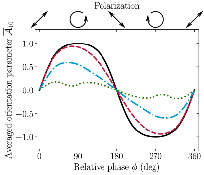
Figure 6: Same as Fig. 4 (c), but for different sizes of the atomic target: $\sigma=0$ (black solid line), $\sigma=20$ nm (red dashed line), $\sigma=50$ nm (blue dash-dotted line), and $\sigma=100$ nm (green dotted line).

IV Summary and Outlook

In summary, we have performed a theoretical analysis of the excitation of a single atom by a combination of azimuthally polarized light beams exhibiting a local isolated magnetic field. Special attention has been paid to magnetic sublevel population of the atom as well as to the question how this population is affected by the relative phase between the beam components. This phase can be attributed to the polarization of the isolated magnetic field at the beam axes intersection. In order to explore the sensitivity to the polarization of such “magnetic light”, we have solved the Liouville–von Neumann equation for the time evolution of the atomic density matrix.

While the formalism developed here can be applied to any atom and transition, in the present study we considered the $2s^{2}2p^{2}\,{}^{3}P_{0}\,-\,2s^{2}2p^{2}\,{}^{3}P_{1}$, the $1s^{2}2s^{2}\,{}^{1}S_{0}\,-\,1s^{2}2s2p\,{}^{3}P_{2}$, and the $2s^{2}2p\;{}^{2}P_{1/2}\,-\,2s^{2}2p\;{}^{2}P_{3/2}$ transitions in ⁴⁰Ca¹⁴⁺, ¹⁰Be, and ³⁸Ar¹³⁺, respectively. Based on the analysis of these transitions, we have shown that different selection rules apply to the excitation by the “magnetic light” compared to conventional plane-wave radiation. In particular, all electric multipole transitions are forbidden when the atomic center of mass is located at the beam axes intersection. For such a localized atom, moreover, the difference of angular momentum projection between the atomic ground and excited state changes within the multipole order in increments of two.

For the $2s^{2}2p\,{}^{2}P_{1/2}\,-\,2s^{2}2p\,{}^{2}P_{3/2}$ transition in ³⁸Ar¹³⁺ we have performed detailed calculations of the atomic population dynamics due to the interaction with “magnetic light”. Based on these calculations we found significant orientation of the ${}^{2}P_{1/2}$ ground state which strongly depends on the relative phase and weights of the azimuthally polarized components. This orientation holds under experimental conditions in which the beam amplitudes differ and the atom is imprecisely localized with respect to intersection of the two beam axes. Following our theoretical results, we propose that analysis of the atomic ground-state orientation can serve as a valuable tool for diagnostics of polarization of optical isolated magnetic fields.

In order to make the proposed scheme more applicable to experiments, a broader theoretical treatment for the interaction of atoms with “magnetic light” is required. In particular, while we restricted our current work to continuous waves of azimuthally polarized light with well-defined phase relationship, we aim to explore the coupling of confined atoms to ultrashort pulses of Laguerre-Gaussian radiation featuring finite laser coherence time in a forthcoming study.

Appendix A Combined electric and magnetic fields

From the vector potential in Eq. (6) and by using the relations $\bm{E}=-\partial_{t}\bm{A}$ and $\bm{B}=\nabla\times\bm{A}$, one can derive the electric and magnetic field of the superposition of azimuthally polarized VB for the geometry shown in Fig. 1. By separating the time-dependent parts, $\bm{E}^{\mathrm{(mag)}}(\bm{r},t)=\bm{E}^{\mathrm{(mag)}}(\bm{r})\mathrm{exp}[-i\omega t]$ and $\bm{B}^{\mathrm{(mag)}}(\bm{r},t)=\bm{B}^{\mathrm{(mag)}}(\bm{r})\mathrm{exp}[-i\omega t]$, the position-dependent terms in the laboratory frame read

$$\begin{split}&\bm{E}^{\mathrm{(mag)}}(\bm{r})\\ =&\,\bm{e}_{x}c_{2}i\omega A_{0}J_{1}(\varkappa\sqrt{x^{2}+z^{2}})\mathrm{exp}[ik_{z}y+i\phi]z/\sqrt{x^{2}+z^{2}}\\ -&\bm{e}_{y}c_{1}i\omega A_{0}J_{1}(\varkappa\sqrt{y^{2}+z^{2}})\mathrm{exp}[ik_{z}x]z/\sqrt{y^{2}+z^{2}}\\ +&\bm{e}_{z}\Bigl(c_{1}i\omega A_{0}J_{1}(\varkappa\sqrt{y^{2}+z^{2}})\mathrm{exp}[ik_{z}x]y/\sqrt{y^{2}+z^{2}}\\ &\;-c_{2}i\omega A_{0}J_{1}(\varkappa\sqrt{x^{2}+z^{2}})\mathrm{exp}[ik_{z}y+i\phi]x/\sqrt{x^{2}+z^{2}}\Bigr),\\ \end{split}$$ (21)

$$\begin{split}&\bm{B}^{\mathrm{(mag)}}(\bm{r})\\ =&\,\bm{e}_{x}\Bigl(c_{1}kA_{0}\sin\theta_{k}J_{0}(\varkappa\sqrt{y^{2}+z^{2}})\mathrm{exp}[ik_{z}x]\\ &\;-c_{2}ikA_{0}\cos\theta_{k}J_{1}(\varkappa\sqrt{x^{2}+z^{2}})\mathrm{exp}[ik_{z}y+i\phi]\\ &\quad\times x/\sqrt{x^{2}+z^{2}}\Bigr)\\ +&\bm{e}_{y}\Bigl(c_{2}kA_{0}\sin\theta_{k}J_{0}(\varkappa\sqrt{x^{2}+z^{2}})\mathrm{exp}[ik_{z}y+i\phi]\\ &\;-c_{1}ikA_{0}\cos\theta_{k}J_{1}(\varkappa\sqrt{y^{2}+z^{2}})\mathrm{exp}[ik_{z}x]\\ &\quad\times y/\sqrt{y^{2}+z^{2}}\Bigr)\\ -&\bm{e}_{z}\Bigl(c_{1}ikA_{0}\cos\theta_{k}J_{1}(\varkappa\sqrt{y^{2}+z^{2}})\mathrm{exp}[ik_{z}x]z/\sqrt{y^{2}+z^{2}}\\ &\,+c_{2}ikA_{0}\cos\theta_{k}J_{1}(\varkappa\sqrt{x^{2}+z^{2}})\mathrm{exp}[ik_{z}y+i\phi]\\ &\quad\times z/\sqrt{x^{2}+z^{2}}\Bigr).\end{split}$$ (22)

References

- edited by J. P. Torres and Torner [2011] edited by J. P. Torres and L. Torner, Twisted Photons: Applications of Light with Orbital Angular Momentum (Wiley, Berlin, 2011).
- Bliokh and Nori [2015] K. Y. Bliokh and F. Nori, Transverse and longitudinal angular momenta of light, Phys. Rep. 592, 1 (2015).
- Barnett et al. [2016] S. M. Barnett, L. Allen, R. P. Cameron, c. R. Gilson, M. J. Padgett, F. C. Speirits, and a. M. Yao, On the natures of the spin and orbital parts of optical angular momentum, J. Opt. 18, 064004 (2016).
- Shen et al. [2023] Y. Shen, Q. Zhan, L. G. Wright, D. N. Christodoulides, F. W. Wise, A. E. Willner, K.-h. Zou, Z. Zhao, M. A. Porras, A. Chong, C. Wan, K. Y. Bliokh, C.-T. Liao, C. Hernández-García, M. Murnane, M. Yessenov, A. F. Abouraddy, L. J. Wong, M. Go, S. Kumar, C. Guo, S. Fan, N. Papasimakis, N. I. Zheludev, L. Chen, W. Zhu, A. Agrawal, M. Mounaix, N. K. Fontaine, J. Carpenter, S. W. Jolly, C. Dorrer, B. Alonso, I. Lopez-Quintas, M. López-Ripa, Í. J. Sola, J. Huang, H. Zhang, Z. Ruan, A. H. Dorrah, F. Capasso, and A. Forbes, Roadmap on spatiotemporal light fields, J. Opt. 25, 093001 (2023).
- Bliokh et al. [2023] K. Y. Bliokh, E. Karimi, M. J. Padgett, M. A. Alonso, M. R. Dennis, A. Dudley, A. Forbes, S. Zahedpour, S. W. Hancock, H. M. Milchberg, S. Rotter, F. Nori, Ş. K. Özdemir, N. Bender, H. Cao, P. B. Corkum, C. Hernández-García, H. Ren, Y. Kivshar, M. G. Silveirinha, N. Engheta, A. Rauschenbeutel, P. Schneeweiss, J. Volz, D. Leykam, D. A. Smirnova, K. Rong, B. Wang, E. Hasman, M. F. Picardi, A. V. Zayats, F. J. Rodríguez-Fortuño, C. Yang, J. Ren, A. B. Khanikaev, A. Alù, E. Brasselet, M. Shats, J. Verbeeck, P. Schattschneider, D. Sarenac, D. G. Cory, D. A. Pushin, M. Birk, A. Gorlach, I. Kaminer, F. Cardano, L. Marrucci, M. Krenn, and F. Marquardt, Roadmap on structured waves, J. Opt. 25, 103001 (2023).
- Allen et al. [1992] L. Allen, M. W. Beijersbergen, R. J. C. Spreeuw, and J. P. Woerdman, Orbital angular momentum of light and the transformation of Laguerre-Gaussian laser modes, Phys. Rev. A 45, 8185 (1992).
- Molina-Terriza et al. [2007] G. Molina-Terriza, J. P. Torres, and L. Torner, Twisted photons, Nat. Phys. 3, 305 (2007).
- Padgett [2017] M. J. Padgett, Orbital angular momentum 25 years on, Opt. Express 25, 11265 (2017).
- Yao and Padgett [2011] A. M. Yao and M. J. Padgett, Orbital angular momentum: origins, behavior and applications, Adv. Opt. Photon. 3, 161 (2011).
- Franke-Arnold [2017] S. Franke-Arnold, Optical angular momentum and atoms, Philos. Trans. R. Soc. A 375, 20150435 (2017).
- Rubinsztein-Dunlop et al. [2017] H. Rubinsztein-Dunlop, A. Forbes, M. V. Berry, M. R. Dennis, D. L. Andrews, M. Mansuripur, C. Denz, C. Alpmann, P. Banzer, T. Bauer, E. Karimi, L. Marrucci, M. J. Padgett, M. Ritsch-Marte, N. M. Litchinitser, N. P. Bigelow, C. Rosales-Guzmán, A. Belmonte, J. P. Torres, T. W. Neely, M. Baker, R. Gordon, A. B. Stilgoe, J. Romero, A. G. White, R. Fickler, A. E. Willner, G. Xie, B. McMorran, and A. M. Weiner, Roadmap on structured light, J. Opt. 19, 013001 (2017).
- Yang et al. [2025] X. Yang, C. Hareau, and M. Mivelle, Twisting Light, Steering Spins: Gold Nanoparticle Magnetization via Inverse Faraday Effect and Orbital Angular Momentum, Nano Lett. 25, 11549–11553 (2025).
- Hall [1996] D. G. Hall, Vector-beam solutions of Maxwell’s wave equation, Opt. Lett. 21, 9 (1996).
- Lax et al. [1975] M. Lax, W. H. Louisell, and W. B. McKnight, From maxwell to paraxial wave optics, Phys. Rev. A 11, 1365 (1975).
- Bliokh et al. [2010] K. Y. Bliokh, M. A. Alonso, E. A. Ostrovskaya, and A. Aiello, Angular momenta and spin-orbit interaction of nonparaxial light in free space, Phys. Rev. A 82, 063825 (2010).
- Quinteiro et al. [2017a] G. F. Quinteiro, F. Schmidt-Kaler, and C. T. Schmiegelow, Twisted-Light–Ion Interaction: The Role of Longitudinal Fields, Phys. Rev. Lett. 119, 253203 (2017a).
- Quinteiro et al. [2017b] G. F. Quinteiro, D. E. Reiter, and T. Kuhn, Formulation of the twisted-light–matter interaction at the phase singularity: Beams with strong magnetic fields, Phys. Rev. A 95, 012106 (2017b).
- Babiker et al. [2019] M. Babiker, D. L. Andrews, and V. E. Lembessis, Atoms in complex twisted light, J. Opt. 21, 013001 (2019).
- Iketaki et al. [2007] Y. Iketaki, T. Watanabe, N. Bokor, and M. Fujii, Investigation of the center intensity of first- and second-order Laguerre–Gaussian beams with linear and circular polarization, Opt. Lett. 32, 2357 (2007).
- Monteiro et al. [2009] P. B. Monteiro, P. A. Maia Neto, and H. Moysés Nussenzveig, Angular momentum of focused beams: Beyond the paraxial approximation, Phys. Rev. A 79, 033830 (2009).
- Klimov et al. [2012] V. V. Klimov, D. Bloch, M. Ducloy, and J. R. Rios Leite, Mapping of focused Laguerre-Gauss beams: The interplay between spin and orbital angular momentum and its dependence on detector characteristics, Phys. Rev. A 85, 053834 (2012).
- Peshkov et al. [2023] A. A. Peshkov, E. Jordan, M. Kromrey, K. K. Mehta, T. E. Mehlstäubler, and A. Surzhykov, Excitation of Forbidden Electronic Transitions in Atoms by Hermite–Gaussian Modes, Ann. Phys. (Berlin) 535, 2300204 (2023).
- Veysi et al. [2015] M. Veysi, C. Guclu, and F. Capolino, Vortex beams with strong longitudinally polarized magnetic field and their generation by using metasurfaces, J. Opt. Soc. Am. B 32, 345 (2015).
- Blanco et al. [2019] M. Blanco, F. Cambronero, M. T. Flores-Arias, E. C. Jarque, L. Plaja, and C. Hernández-García, Ultraintense Femtosecond Magnetic Nanoprobes Induced by Azimuthally Polarized Laser Beams, ACS Photonics 6, 38 (2019).
- Martín-Hernández et al. [2024] R. Martín-Hernández, L. Grünewald, L. Sánchez-Tejerina, L. Plaja, E. C. Jarque, C. Hernández-García, and S. Mai, Optical magnetic field enhancement using ultrafast azimuthally polarized laser beams and tailored metallic nanoantennas, Photon. Res. 12, 1078 (2024).
- Sederberg et al. [2020] S. Sederberg, F. Kong, and P. B. Corkum, Tesla-scale terahertz magnetic impulses, Phys. Rev. X 10, 011063 (2020).
- Reynier et al. [2023] B. Reynier, E. Charron, O. Markovic, X. Yang, B. Gallas, A. Ferrier, S. Bidault, and M. Mivelle, Full control of electric and magnetic light–matter interactions through a nanomirror on a near-field tip, Optica 10, 841 (2023).
- Reynier et al. [2025] B. Reynier, E. Charron, O. Markovic, B. Gallas, A. Ferrier, S. Bidault, and M. Mivelle, Nearfield control over magnetic light-matter interactions, Light: Science & Applications 14, 127 (2025).
- Veysi et al. [2016] M. Veysi, C. Guclu, and F. Capolino, Focused azimuthally polarized vector beam and spatial magnetic resolution below the diffraction limit, J. Opt. Soc. Am. B 33, 2265 (2016).
- Wózniak and Banzer [2021] P. Wózniak and P. Banzer, Single nanoparticle real and k-space spectroscopy with structured light, New J. Phys. 23, 103013 (2021).
- Zeng et al. [2023] J. Zeng, Y. Dong, J. Zhang, and J. Wang, The trend of structured light-induced force microscopy: a review, J. Opt. 25, 023001 (2023).
- Kasperczyk et al. [2015] M. Kasperczyk, S. Person, D. Ananias, L. D. Carlos, and L. Novotny, Excitation of magnetic dipole transitions at optical frequencies, Phys. Rev. Lett. 114, 163903 (2015).
- Sánchez-Tejerina et al. [2023] L. Sánchez-Tejerina, R. Martín-Hernández, R. Yanes, L. Plaja, L. López-Díaz, and C. Hernández-García, All-optical nonlinear chiral ultrafast magnetization dynamics driven by circularly polarized magnetic fields, High Pow. Laser Sci. Eng. 11, e82 (2023).
- Tang and Cohen [2010] Y. Tang and A. E. Cohen, Optical chirality and its interaction with matter, Phys. Rev. Lett. 104, 163901 (2010).
- Cheong and Xu [2022] S.-W. Cheong and X. Xu, Magnetic chirality, npj Quantum Materials 7, 40 (2022).
- Martín-Domene et al. [2024] S. Martín-Domene, L. Sánchez-Tejerina, R. Martín-Hernández, and C. Hernández-García, Generation of intense, polarization-controlled magnetic fields with non-paraxial structured laser beams, App. Phys. Lett. 124, 211101 (2024).
- Kuznetsov et al. [2012] A. I. Kuznetsov, A. E. Miroshnichenko, Y. H. Fu, J. Zhang, and B. Luk’yanchuk, Magnetic light, Sci. Rep. , 492 (2012).
- Jentschura and Serbo [2011] U. D. Jentschura and V. G. Serbo, Generation of High-Energy Photons with Large Orbital Angular Momentum by Compton Backscattering, Phys. Rev. Lett. 106, 013001 (2011).
- Matula et al. [2013] O. Matula, A. G. Hayrapetyan, V. G. Serbo, A. Surzhykov, and S. Fritzsche, Atomic ionization of hydrogen-like ions by twisted photons: angular distribution of emitted electrons, J. Phys. B 46, 205002 (2013).
- Knyazev and Serbo [2018] B. A. Knyazev and V. G. Serbo, Beams of photons with nonzero projections of orbital angular momenta: new results, Phys.-Usp. 61, 449 (2018).
- Schulz et al. [2020] S. A.-L. Schulz, A. A. Peshkov, R. A. Müller, R. Lange, N. Huntemann, C. Tamm, E. Peik, and A. Surzhykov, Generalized excitation of atomic multipole transitions by twisted light modes, Phys. Rev. A 102, 012812 (2020).
- Rose [1957] M. E. Rose, Elementary Theory of Angular Momentum (John Wiley & Sons, New York, 1957).
- Akhiezer and Berestetskii [1965] A. I. Akhiezer and V. B. Berestetskii, Quantum Electrodynamics (John Wiley & Sons, New York, 1965).
- Goren et al. [2004] C. Goren, A. D. Wilson-Gordon, M. Rosenbluh, and H. Friedmann, Atomic four-level systems, Phys. Rev. A 69, 053818 (2004).
- Johnson [2007] W. R. Johnson, Atomic Structure Theory (Springer, New York, 2007).
- von der Wense et al. [2020] L. von der Wense, P. V. Bilous, B. Seiferle, S. Stellmer, J. Weitenberg, P. G. Thirolf, A. Pálffy, and G. Kazakov, The theory of direct laser excitation of nuclear transitions, Eur. Phys. J. A 56, 176 (2020).
- Varshalovich et al. [1988] D. A. Varshalovich, A. N. Moskalev, and V. K. Khersonskii, Quantum Theory of Angular Momentum (World Scientific Publishing Co. Pte. Ltd., Singapore, 1988).
- Auzinsh et al. [2010] M. Auzinsh, D. Budker, and S. M. Rochester, Optically Polarized Atoms: Understanding Light-Atom Interactions (Oxford University, Oxford, 2010).
- Blum [2012] K. Blum, Density Matrix Theory and Applications (Springer, Berlin, 2012).
- Tremblay and Jacques [1990] P. Tremblay and C. Jacques, Optical pumping with two finite linewidth lasers, Phys. Rev. A 41, 4989 (1990).
- Schmidt et al. [2024] R. P. Schmidt, S. Ramakrishna, A. A. Peshkov, N. Huntemann, E. Peik, S. Fritzsche, and A. Surzhykov, Atomic photoexcitation as a tool for probing purity of twisted light modes, Phys. Rev. A 109, 033103 (2024).
- Ramakrishna et al. [2024] S. Ramakrishna, R. P. Schmidt, A. A. Peshkov, S. Franke-Arnold, A. Surzhykov, and S. Fritzsche, Interaction of vector light beams with atoms exposed to a time-dependent magnetic field, Phys. Rev. A 110, 043101 (2024).
- Balashov et al. [2000] V. V. Balashov, A. N. Grum-Grzhimailo, and N. M. Kabachnik, Polarization and Correlation Phenomena in Atomic Collisions: A Practical Theory Course, edited by P. G. Burke and H. Kleinpoppen (Springer-Verlag, Berlin, 2000).
- Naqvi [1951] A. M. Naqvi, Mutual magnetic interactions in p-electron configurations (with calculations of transition probabilities and astrophysical applications), Ph.D. thesis, Harvard University (1951).
- Tachiev and Froese Fischer [1999] G. Tachiev and C. Froese Fischer, Breit-pauli energy levels, lifetimes, and transition data: beryllium-like spectra, J. Phys. B: At. Mol. Opt. Phys. 32, 5805 (1999).
- Rynkun et al. [2012] P. Rynkun, P. Jönsson, G. Gaigalas, and C. Froese Fischer, Energies and E1, M1, E2, M2 transition rates for states of the 2s22p, 2s2p2, and 2p3 configurations in boron-like ions between N III and Zn XXVI, Atomic Data and Nuclear Data Tables 98, 481 (2012).
- Fox [2006] M. Fox, Quantum Optics: An Introduction (Oxford University Press, Oxford, 2006).
- Blatt and Zoller [1988] R. Blatt and P. Zoller, Quantum jumps in atomic systems, Eur. J. Phys. 9, 250 (1988).
- Schmiegelow et al. [2016] C. T. Schmiegelow, J. Schulz, H. Kaufmann, T. Ruster, U. G. Poschinger, and F. Schmidt-Kaler, Transfer of optical orbital angular momentum to a bound electron, Nat. Commun. 7, 12998 (2016).
- Lange et al. [2022] R. Lange, N. Huntemann, A. A. Peshkov, A. Surzhykov, and E. Peik, Excitation of an Electric Octupole Transition by Twisted Light, Phys. Rev. Lett 129, 253901 (2022).
- Duan et al. [2019] Y. Duan, R. A. Müller, and A. Surzhykov, Selection rules for atomic excitation by twisted light, J. Phys. B: At. Mol. Opt. Phys. 52, 184002 (2019).