An Accurate Comprehensive Approach to Substructure:
IV. Dynamical Friction

Abstract

In three previous Papers we analysed the origin of the properties of halo substructure found in simulations. This was achieved by deriving them analytically in the peak model of structure formation, using the statistics of nested peaks (with no free parameter) plus a realistic model of subhalo stripping and shock-heating (with only one parameter). However, to simplify the treatment we neglected dynamical friction (DF). Here, we revisit that work by including it. That is done in a fully analytic manner, i.e. avoiding the integration of subhalo orbital motions. This leads to simple accurate expressions for the abundance and radial distribution of subhaloes of different masses, which disentangle the effects of DF from those of tidal stripping and shock-heating. This way we reproduce and explain the results of simulations and extend them to haloes of any mass, redshift and formation times in the desired cosmology.

1 INTRODUCTION

Dynamical friction (DF) plays an important role in the evolution of many self-gravitating systems such as massive stars in young galaxies (Raveh et al. 2021), spiral arms in disc galaxies (Sellwood 2021; Chiba 2023), stars in globular clusters (Shi, Grudić, & Hopkins 2021; Bhattacharyya & Singh Bagla 2023), globular clusters in dwarf galaxies (Li et al. 2021; Borukhovetskaya et al. 2022; Shao et al. 2021), black hole binaries (Berezhiani et al. 2023), super massive black holes in galaxies (Ma et al. 2021; Rawlings et al. 2023; DeGraf et al. 2023) and primordial black holes (Sureda et al. 2021; Stasenko & Belotsky 2023). Unfortunately, the absence of a fully analytic treatment of DF complicates their modelling.

That is the case in particular of substructure in cold dark matter (CDM) haloes (e.g., Lacey & Cole 1993; Taylor & Babul 2001; Benson et al. 2002). Due to he complexity of the problem, involving the subhalo aggregation history and their evolution through tidal-stripping, shock heating and DF as they orbit inside the host haloes, the usual way to address it has been by means of high-resolution cosmological $N$-body simulations (e.g. Diemand et al. 2007; Springel et al. 2008; Angulo et al. 2009; Elahi et al. 2009; Boylan-Kolchin et al. 2010; Giocoli et al. 2010; Klypin et al. 2011; Gao et al. 2011, 2012; Onions et al. 2012; Lovell et al. 2014; Cautun et al. 2014b; Ishiyama et al. 2020), recently taking into account the hydrodynamics of gas (e.g. Richings et al. 2020; Font et al. 2020; Font, McCarthy, & Belokurov 2020; Hellwing et al. 2016; Bose et al. 2016, 2020). But this approach is very CPU time-consuming, so the properties of substructure are only known for a few haloes with specific aggregation histories. In addition, simulations do not facilitate a detailed understanding of how these properties are set. This is why (semi) analytic models (e.g. Taylor & Babul 2001; Fujita et al. 2002; Zentner & Bullock 2003; Sheth 2003; Lee 2004; Oguri & Lee 2004; Taylor & Babul 2004; Peñarrubia et al. 2004; van den Bosch et al. 2005; Zentner et al. 2005; Kampakoglou & Benson 2007; Giocoli et al. 2008; Angulo et al. 2009; Benson et al. 2013; Pullen et al. 2014; Jiang & van den Bosch 2016; Griffen et al. 2016; van den Bosch & Jiang 2016; van den Bosch et al. 2018; Green & van den Bosch 2019; Jiang et al. 2021) have also been used. Unfortunately, in the absence of an analytic treatment of DF (see the work in this direction by Buehler & Desjacques 2023), analytic models must integrate the subhalo orbital motion, which is similarly CPU time-consuming. What is worse, the numerical integration of orbits deprives the models from their main reason to be: finding simple analytic expressions facilitating the comprehension of the problem and describing the general case.

In (Salvador-Solé et al., 2021a, b, c), hereafter Papers I, II and III, respectively, we built a very detailed analytic model of halo substructure in the peak model, based on the powerful ConflUent System of Peak trajectories (CUSP) formalism (Manrique & Salvador-Solé, 1995, 1996; Manrique et al., 1998) having also allowed us to derive analytically all the remaining inner halo properties (Salvador-Solé & Manrique 2021 and references therein), their clustering (Salvador-Solé & Manrique, 2024; Salvador-Solé et al., 2024) and angular momentum growth (Salvador-Solé et al., 2025)). In those Papers we were able to reproduce and explain the abundance or mass function (MF) and radial distribution of accreted non-evolved subhaloes (Paper I) and evolved ones through the action of tidal stripping and shock-heating (Paper II) in both purely accreting and ordinary haloes of different masses, redshifts and aggregation histories (Paper III). However, to facilitate the analytic treatment we neglected DF, so the results obtained only held for low mass subhaloes because.

In this Paper we remedy that limitation. We revisit the study by including DF, treated in a fully analytic manner. This allows us to obtain simple analytic expressions for the subhalo MF and radial distribution showing how DF alters the results derived in Papers II and III. This way, we disentangle the role of all the different processes shaping the properties of halo substructure found in simulations and extend them to haloes of any mass, redshift, and formation time in any desired CDM cosmology.

The layout of the Paper is as follows. In Section 2 we study the effect of DF on individual subhaloes. In Section 3 we implement the results to the entire subhalo population of purely accreting haloes and real ones having undegone major mergers. The summary and concluding remarks are given in Section 4. To facilitate the comparison with the results of Papers I, II and III (and of simulations) all Figures in the Paper are for the WMAP7 (Komatsu et al., 2011) cosmology and Milky Way (MW) mass haloes.

2 Individual Subhaloes

There are in the literature two different mechanisms referred to DF. One is that caused by the local wake produced by light particles of a continuous medium scattered behind an object moving inside it. This mechanism, introduced by Chandrasekhar (1943), causes the velocity loss and orbital decay of subhaloes (Bekenstein, 1989; Mulder, 1983; Colpi & Pallavicini, 1998; Colpi et al., 1999; Binney & Tremaine, 2008). But the torque produced by the long-scale resonant interaction of a moving subhalo with the host halo also contributes to its orbital decay (White, 1983; Tremanine & Weinberg, 1984; Weingerg, 1986, 1989; Choi et al., 09; Ogiya & Burkert, 2016; Garavitoi-Camargo et al., 2019; Cunningham et al., 2020; Tamfal et al., 2021). This is why this latter mechanism is also called global mode DF even though it does not really behave as a friction. Tamfal et al. (2021) showed that, when there is one only very massive subhalo, this global mode DF is stronger than the former local one. However, very massive ones undergo very strong DF of the former kind and fall into the centre of the host halo in one (long) orbit and disappear, while the global mode DF does not take place during the first orbit of a subhalo (Tamfal et al., 2021). Thus, we concentrate from now on in the effects of local DF.

The equation of motion of a subhalo with mass $M_{\rm s}$ orbiting within a spherical halo of mass $M_{\rm h}$ at some cosmic time $t_{\rm h}$, subject to the action of the local wake DF is

$$\ddot{\bf r}=-\nabla\Phi(r)-A(v,r,M_{\rm s})\dot{\bf r},$$ (1)

where ${\bf r}$ is the position vector of the subhalo with origin at the centre of the halo, $\Phi(r)$ is the gravitational potential and $A$ is the (positive) DF coefficient (Chandrasekhar, 1943), well approximated in finite spherical systems by (e.g. Peñarrubia et al. 2010; Jiang et al. 2021)

$$A(v,r,M_{\rm s})=4\pi\,G^{2}\,M_{\rm s}\,\rho(r)\,f_{\rm dDM}(r)\,\ln\Lambda\,\frac{F(<v)}{v^{3}}.$$ (2)

For simplicity in the notation, here and in what follows, we skip the arguments $M_{\rm h}$ and $t_{\rm h}$ referring to the mass and time of the halo. They will only be included in Section 3.2 when dealing with haloes of different masses and times.

In equation (2), $G$ is the gravitational constant, $\ln\Lambda$ is the so-called Coulomb logarithm (see ther discussion below), $v$ is the modulus of $\dot{\bf{r}}$, $F(<v)$ is the fraction of particles with relative velocities less than $v$, equal to erf$(X)-(2/\sqrt{\pi})X\exp(-X^{2})$, where $X\equiv\sqrt{3/2}\,v/\sigma(r)$, $\sigma(r)$ and $\rho(r)$ are the isotropic (3D) velocity dispersion and density profiles of the host halo and $f_{\rm dDM}(r)$ is the diffuse dark matter (dDM) mass fraction profile. As mentioned, as long as haloes are accreting, they grow inside-out (Salvador-Solé et al., 2012a), so the local density and velocity dispersion at any fixed radius stay essentially unaltered. Strictly speaking, the dDM fraction $f_{\rm dDM}(r)$ slightly increases with time as subhalo stripping progresses (Salvador-Solé et al., 2021b) and the density profile of haloes slightly deepens as a consequence of DF acting on massive subhaloes. However, for simplicity, these minor effects are ignored.

The Coulomb logarithm is a fudge factor introduced to adapt the Chandrasekhar (1943) formula originally derived by Chandrasekhar (1943) for homogeneous infinite systems to finite ones with some particular geometry. There are different more or less complicate forms in the literature for that factor (e.g. Read et al. 2006; Gan et al. 2010; Taylor & Babul 2001; Peñarrubia & Benson 2005; Arena & Bertin 2007; Peñarrubia et al. 2010). From now on we will assume for simplicity that it does not depend on $r$ and $v$, with a constant value of 2.1 as shown to reasonably reproduce the results of simulations for spherical pure CDM haloes endowed with density profiles of the typical NFW (Navarro, Frenk & White, 1995) form (Peñarrubia & Benson, 2005; Arena & Bertin, 2007; Peñarrubia et al., 2010). Note also that in equation (2) we have neglected the DF caused by less massive subhaloes as it is much less marked than that caused by dDM.

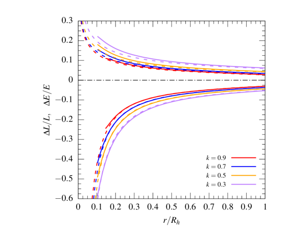
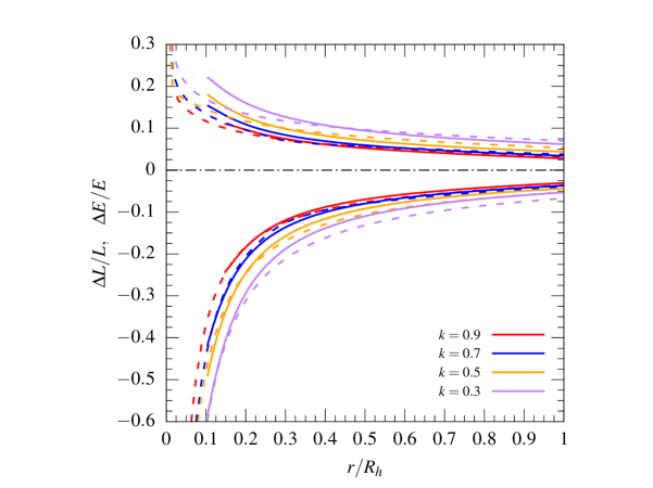
Figure 1: Approximate relative energy $E$ and angular momentum $L$ increments (positive and negative, respectively) as a function of the radius $r$ (scaled to the virial radius $R_{\rm h}$ of the halo) and several fixed values of $k$ measuring the initial velocity at apocentre M_⊙ (dashed lines) for subhaloes of mass $M_{\rm s}=10^{-2}M_{\rm h}$ in current MW mass haloes, compared to the exact results obtained by integration over real orbital motions with DF (solid lines). The black dot-dashed line marks the zero baseline. Left panel: Approximate $\Delta E/E$ and $\Delta L/L$ values obtained by integration over virtual orbits with no DF. Right panel: Approximate purely analytic $\Delta E/E$ and $\Delta L/L$ values (i.e. obtained with no integration).
(A colour version of this Figure is available in the online journal.)

2.1 One Orbit

Next, in a first step we calculate the effect of DF alone and, in a second step, its combined effect with tidal stripping and shock-heating.

2.1.1 DF only

Multiplying equation (1) by $\dot{\bf r}$ and integrating over one orbit, we obtain

$$E(r^{\rm f})=E(r)+\Delta E,$$ (3)

where $E$ is the total energy of the subhalo, $r$ and $r^{\rm f}$ are the initial and final apocentric radii, respectively, and

$$\Delta E=\!-M_{\rm s}\!\int_{0}^{T}\!\!A[v(t),r(t),M_{\rm s}]v^{2}(t){\rm d}t\equiv\!-M_{\rm s}A_{\rm E}\!\int_{0}^{T}\!\!v^{2}{\rm d}t,$$ (4)

with $T$ being the orbital period, dependent on the subhalo apocentric radius, (tangential) velocity and mass, and $A_{\rm E}$ being the energy-averaged DF coefficient over one orbit.

On the other hand, since the momentum of a central force is null, the direction of the angular momentum of the subhalo relative to the centre of the halo, ${\bf L}=M_{\rm s}{\bf r}\times{\bf\dot{r}}$, with $\ddot{\bf r}$ given by equation (1), is kept constant and the time-derivative of its modulus is simply $-AL$, so, integrating it over one orbit, we find

$$L(r^{\rm f})=L(r)+\Delta L,$$ (5)

where

$$\Delta L=-L\left(1-\exp{\left\{-\int_{0}^{T}A[v(t),r(t),M_{\rm s}]{\rm d}t\right\}}\right)~~~~~~~~$$

$$=-L\int_{0}^{T}A[v(t),r(t),M_{\rm s}]{\rm d}t\equiv-LA_{\rm L}T,~~~~~~~~~~~~~~~$$ (6)

with $A_{\rm L}$ being the angular momentum-averaged DF coefficient over one orbit. Equation (6) holds to first order in the effects of DF as most equations throughout this Paper, but, for simplicity, we write from now on the symbol $=$ and reserve the symbol $\approx$ for the case of some additional approximation.

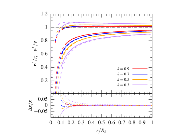
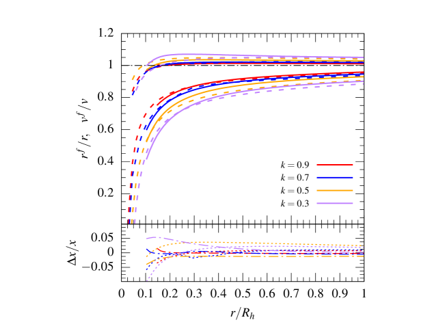
Figure 2: Ratios of final to initial radii (curves below unity) and tangential velocities (curves above unity) at apocentre in one orbit found by numerical integration of the orbital motion of subhaloes (solid lines) and obtained to first order in the relative energy and angular momentum increments, $\Delta E/E$ $\Delta L/L$ (dashed lines), as a function of $r$ for several $k$ values and the same $M_{\rm s}$, $M_{\rm h}$ and $t_{\rm h}$ as in Figure 1. Again, the black dot-dashed line marks the zero value. In the bottom panel we plot the relative differences between the approximations values (dotted lines for apocentric radii and dot-dashed lines for tangential velocities) and the exact solutions (the zero baseline). Left panels: Results obtained using the leading-order-approximate $\Delta E/E$ and $\Delta L/L$ increments found by integration over virtual orbits with no DF. Right panels: Results obtained using the approximate purely analytic $\Delta E/E$ and $\Delta L/L$ values.
(A colour version of this Figure is available in the online journal.)

In Appendix A we calculate the relative increments $\Delta E/E$ and $\Delta L/$, positive and negative, respectively, as functions of the initial apocentric radius $r$ and (tangential) velocity $v$ or, equivalently, the parameter $k\equiv v^{2}/GM(r)/r$, where $\sqrt{GM(r)/r}$ is the circular velocity ($k\leq 1$). The calculation is achieved in two different ways: 1) a first one accurate to leading order in the effects of DF, in which the integrals in equations (4) and (6) are carried out over the well-known orbits without DF, i.e. with no need to solve the equation of motion of subhaloes with DF, and 2) a second less accurate though fully analytic one involving no integral at all.

Both versions of $\Delta E/E$ and $\Delta L/L$ are compared in Figure 1 to the exact values of these quantities found by numerical integration over the real subhalo orbit with DF. The solid lines giving the exact $\Delta E/E$ and $\Delta L/L$ values are truncated at $r\la 0.1$. At smaller $r$, subhaloes spiral down to the halo centre without reaching any new apocentre, so the definition of the orbital period $T$ as the time between two consecutive apocentres becomes meaningless. (The same situation is found for $k$ close to unity; in Figure 1 that happens at $k>0.9$.) Defining $T$ at those radii as the time spent until the subhalo reaches the halo centre is not a solution because this would yield a large discontinuity in those lines. The best solution is to define the orbital period at those radii ($k$ values) by continuity with the values found at larger $r$ for the same $k$ (at smaller $k$ for the same $r$). This is what we have done for approximate $\Delta E/E$ and $|\Delta L/L|$ values (dashed lines). Had we adopted the same definition for the exact $\Delta E/E$ and $|\Delta L/L|$ values, the comparison of the dashed lines to the solid ones at small $r$ (large $k$) would be similarly good. In what follows we use such an extended orbital period.

The changes in one orbit of the apocentric radius $r$ with (tangential) velocity $v$ to the final ones, $r^{\rm f}$ and $v^{\rm f}$, can be calculated to first order in $\Delta E/E$ and $\Delta L/L$, writing the particle velocity at apocentre in terms of the radius and the angular momentum and Taylor expanding to first order the potential at the final radius $\Phi(r^{\rm f})$ around the initial one $r$. This leads to a cubic equation for the ratio $Q^{\rm f}\equiv r^{\rm f}/r$, whose result is

$$Q^{\rm f}\!=\!1+\frac{k}{1-k}\!\left[\frac{S(k,r)}{2}\frac{\Delta E}{E}(k,r,M_{\rm s})-\frac{\Delta L}{L}(k,r,M_{\rm s})\right]\!,$$ (7)

with $S(k,r)\equiv 1+2r\Phi(r)/[kGM(r)]=1-2/k\ln[1+c(r)]/f[c(r)]<0$, leading to

$$\frac{r^{\rm f}}{r}=Q^{\rm f}(k,r,M_{\rm s})\,~~~~~~~~~~~~~~~~~~~~~~~~~~~~~~~~~~~~~~~~~~~~~~~~~~$$ (8)

$$\frac{v^{\rm f}}{v}=\frac{1+\frac{\Delta L}{L}(k,r,M_{\rm s})}{Q^{\rm f}(k,r,M_{\rm s})}.\!~~~~~~~~~~~~~~~~~~~~~~~~~~~~~~~~~~~~~~~~~~~$$ (9)

In Figure 2 we compare the ratios $r^{\rm f}/r$ and $v^{\rm f}/v$ obtained from the two approximate versions of $\Delta E/E$ and $\Delta L/L$ to the exact values obtained by numerical integration. As can be seen, the most accurate estimates of $\Delta E/E$ and $\Delta L/L$ lead to $r^{\rm f}/r$ and $v^{\rm f}/v$ ratios that almost fully recover the exact ones at all $r$ and $k$. But, even the less accurate fully analytic estimates of $\Delta E/E$ and $\Delta L/L$ give very good results, so we adopt them in what follows.

Certainly, equations (8) and (9) hold to first order in the quantities $\Delta E/E$ and $\Delta L/L$, which are proportional to $M_{\rm s}$ (see App. A), so those values of $r^{\rm f}/r$ and $v^{\rm f}/v$ might not be accurate enough for massive subhaloes suffering strong DF. But this is not the case. As long as $r^{\rm f}/r$ is non-null, equations (8) and (9) give fairly good estimates of the exact $r^{\rm f}/r$ and $v^{\rm f}/v$ values regardless of the subhalo mass (see Figs. 1 and 2). While, when $r^{\rm f}/r$ vanishes, the subhalo falls into the halo centre, merges with the central dark matter lump and disappears (see Paper II), so we must no longer monitor its orbital motion. Therefore, equations (8) and (9) can be safely applied for all subhalo masses.

2.1.2 DF Combined with Stripping and Shock-Heating

Although tides operate over the entire subhalo orbit, their most marked effect takes place at the pericentric radius, $r_{\rm per}$. Before that, the softly stripped material stays close to the subhalo, so the DF produced on the subhalo and its stripped matter is the same as if the subhalo had not been stripped. In contrast, at pericentre the (cumulative and new) stripped material substantially separates from the subhalo due to the shock heating produced at that point, so, its way back to the apocentre, DF acts on the subhalo according to its new mass. Until reaching the new apocentre, the subhalo is kept essentially unchanged because the stripped subhalo has no time to relax and with that shape the stripping is not so marked as at pericentre. Only when the subhalo is near the apocentre has the subhalo enough time to relax and its structure acquires a new state of equilibrium with which it begins a new orbit.

As shown in Paper II, for subhaloes at the apocentric radius $r$, with velocity $v$, mass $M_{\rm s}$ and a NFW density profile with concentration $c_{\rm s}$, the relative truncated radius $Q_{\rm s}^{\rm tr}(v,r,M_{\rm s})\equiv R_{\rm s}^{\rm tr}(v,r,M_{\rm s})/R_{\rm s}$ after stripping and shock-heating at pericentre satisfies

$$\frac{f(c_{\rm s}Q_{\rm s}^{\rm tr})}{f(c_{\rm s})(Q_{\rm s}^{\rm tr})^{3}}=\frac{f\left[c(r)Q_{\rm per}(v,r,M_{\rm s})\right]}{f[c(r)]Q_{\rm per}^{3}(v,r,M_{\rm s})},$$ (10)

with $f(x)=\ln(1+x)-x/(1+x)$. The truncated mass $M_{\rm s}^{\rm tr}$ satisfies in turn

$$\frac{M_{\rm s}^{\rm tr}}{M_{\rm s}}=\frac{f\left(c_{\rm s}Q_{\rm s}^{\rm tr}\right)}{f(c_{\rm s})}=\frac{f\left[c(r)Q_{\rm per}(v,r,M_{\rm s})\right]}{f[c(r)]Q_{\rm per}^{3}(v,r,M_{\rm s})}(Q_{\rm s}^{\rm tr})^{3},$$ (11)

where $c(r)$ is the concentration of the part of the host halo with mass $M(r)$ and, hence, radius $r$ (i.e., $c(r)=rc_{\rm h}/R_{\rm h}<c_{\rm h}$, with $c_{\rm h}$ being the concentration of the halo at $t_{\rm h}$) and $Q_{\rm per}$ is defined as $r_{\rm per}/r$. In the absence of DF, $Q_{\rm per}$ does not depend on $M_{\rm s}$, so, as $c_{\rm s}$ is weakly dependent on $M_{\rm s}$, $Q_{\rm s}^{\rm tr}$ is also essentially independent of $M_{\rm s}$ (see eq. [10]). However, in the presence of DF, $r_{\rm per}^{\rm f}$ depends on $M_{\rm s}$ and $Q_{\rm per}$ becomes $Q_{\rm per}^{\rm f}$, which also depends on $M_{\rm s}$, so the final subhalo radius $Q_{\rm s}^{\rm f}=R^{\rm f}/R$ does too. This is the difference introduced by DF in the stripping model of Paper II.

To calculate the mass $M^{\rm f}$ of the stripped subhalo in the presence of DF we need the ratio $Q_{\rm per}^{\rm f}=r_{\rm per}^{\rm f}/r$. The relation between the modified and original pericentric radii, $r_{\rm per}^{\rm f}$ and $r_{\rm per}$, is obviously the same as between the modified and original apocentric radii (eq. [8]) after one orbit. But the deviation of $r_{\rm per}^{\rm f}$ from $r_{\rm per}$ after half one orbit (i.e. since the previous apocentre at $r$) is given by $r_{\rm per}^{\rm f}/r_{\rm per}$ equal to $Q^{\rm f}$ (eq. [7]) for $\Delta E/E$ and $\Delta L/L$ corresponding to half the period $T$ (or, equivalently, corresponding to the whole period though half the mass $M_{\rm s}$; see App. A). And, using the approximation $r_{\rm per}/r\approx\tilde{k}\equiv k(1+\sqrt{1+8/k})/4$ (see App. A), we obtain

$$Q_{\rm per}^{\rm f}(k,r,M_{\rm s})\equiv\frac{r_{\rm per}^{\rm f}}{r}\approx\tilde{k}\,Q^{\rm f}(k,r,M_{\rm s}/2).$$ (12)

To write equation (12) we have taken into account that $Q^{\rm f}$ (eq. [7]) for $\Delta L/L$ and $\Delta E/E$ corresponding to half the period $T$ and mass $M_{\rm s}$ equals $Q^{\rm f}$ for the whole period $T$ and the mass $M_{\rm s}/2$ (see eqs. [56] and [57]). Note that the effective values of $A_{\rm E}$ and $A_{\rm L}$ averaged over half the period (from apocentre to pericentre) are indeed the same as averaged over the full orbit (see eqs. [4] and [6]).

After stripping at pericentre, the subhalo ends its orbit with the stripped mass $M_{\rm s}^{\rm f}$. Since half the orbit is carried with the original mass $M_{\rm s}$ and the other half with the stripped mass $M_{\rm s}^{\rm f}$, the changes produced in the apocentre after completing the orbit with stripping at the pericentre coincide with the arithmetic mean of those produced with DF only over the orbit of the subhalo with the two masses. Lastly, when the subhalo reaches the apocentre, it settles in a new equilibrium state, with NFW density profile though a somewhat larger concentration $c_{\rm s}^{\rm f}$ so that, in its next orbit, it will be further stripped and heated (see Sec. 2.2). In the impulsive approximation and no DF, the new concentration is related to the original one through (Paper II)

$$\frac{h(c_{\rm s}^{\rm tr})}{h(c_{\rm s})}=\kappa\left(\frac{M_{\rm s}^{\rm tr}}{M_{\rm s}}\right)^{\beta+5/6},$$ (13)

where $h(c)\equiv f(c)(1+c)/\{c^{3/2}[3/2-s^{2}(c)]^{1/2}\}$, being $s^{2}(c)$ the isotropic 3D velocity variance $\sigma^{2}$ scaled to $cf(c)GM/R$ of a halo with mass $M_{\rm h}$, total radius $R_{\rm h}$ and concentration $c$. And, in the presence of DF, the same derivation leads to equation (13) with $c_{\rm s}^{\rm tr}$ and $M_{\rm s}^{\rm tr}$ replaced by $c_{\rm s}^{\rm f}$ and $M_{\rm s}^{\rm f}$ resulting from the combined action of DF and stripping plus shock-heating. Constants $\kappa=0.77$ and $\beta=-1/2$ give very good fits to the results of numerical experiments (Paper II).

2.2 Multiple Concatenated Orbits

To calculate the final truncated mass and radius of subhaloes with original mass $M_{\rm s}$ accreted by the halo when its mass was $M(r)$ we must calculate in an iterative way the changes produced in successive orbits since $t(r)$.

The stripping and shock-heating of subhaloes depend on the concentration $c(r)=r/r_{\rm s}$ of the host halo at $t(r)$, where $r_{\rm s}$ is the core radius of the halo at $t_{\rm h}$, and on the properties of subhaloes at accretion. After turnaround they fall onto the halo and start orbiting and being stripped and heated, so their mass $M_{\rm s}$ when their apocentre settles down at $r$ is somewhat smaller than the mass $M_{\rm s}^{\rm ntr}$ they would have, had they evolved freely until then. Since during virialisation subhalo velocities vary randomly regardless of their mass, all subhaloes at $r$ must have the same velocity distribution (Jiang et al., 2015). Thus, their typical scaled truncation radius $Q_{\rm s}(r,M_{\rm s}^{\rm ntr})$ can be derived from equation (10), taking the initial subhalo concentration $c_{\rm s}^{\rm ntr}(r,M_{\rm s}^{\rm ntr})$ given by the typical mass-concentration ($M$–$c$) relation for subhaloes with $M_{\rm s}^{\rm ntr}$ at $t(r)$ and the quantity $Q_{\rm per}(r,M_{\rm s}^{\rm ntr})$ equal to twice the velocity-averaged value (for the velocity distribution given in Paper II) of subhaloes at $r$ and $t(r)$. Then, plugging the solution $Q_{\rm s}(r,M_{\rm s}^{\rm ntr})$ in equation (11), we obtain $M_{\rm s}(r,M_{\rm s}^{\rm ntr})/M_{\rm s}^{\rm ntr}$ and, using equation (13), we are led to the concentration $c_{\rm s}(r,M_{\rm s}^{\rm ntr})$ of accreted subhaloes.

These are the initial values of the subhalo properties $r$, $v$, $k$, $M_{\rm s}$, $Q_{\rm s}$ and $c_{\rm s}$ at $t(r)$, which we denote with index 0, i.e., $r_{0}$, $v_{0}$, $k_{0}$, $M_{0}$, $Q_{0}$ and $c_{0}$, respectively. After the first orbit, the subhalo reaches the new apocentric radius $r_{1}$ and velocity $v_{1}$ given by equations (8)-(9) for the mass $(M_{0}+M_{1})/2$, with the mass $M_{1}$ given by equation (11), factor $Q_{1}$ given by equation (10) and concentration $c_{1}$ given by equation (13). After that, the subhalo starts a new orbit.

In general, after $i+1$ orbits, the subhalo with $r_{i}$ and $v_{i}$ given by

$$\frac{r_{i+1}}{r_{i}}=\frac{1}{2}\,\left[Q^{\rm f}(k_{i},r_{i},M_{i})+Q^{\rm f}(k_{i},r_{i},M_{i+1})\right]~~~~~~~~~~~~~~$$ (14)

$$\frac{v_{i+1}}{v_{i}}\!=\!\frac{1}{2}\!\left[\!\frac{1+\frac{\Delta L}{L}(k_{i},r_{i},M_{i})}{Q^{\rm f}(k_{i},r_{i},M_{i})}+\frac{1+\frac{\Delta L}{L}(k_{i},r_{i},M_{i+1})}{Q^{\rm f}(k_{i},r_{i},M_{i+1}}\right].~$$ (15)

with

$$\frac{M_{i+1}}{M_{i}}=\frac{f\left(c_{i}Q_{i+1}\right)}{f(c_{i})},$$ (16)

where $Q_{i+1}$ and $c_{i}$ are given by

$$\frac{f(c_{i}Q_{i+1})}{f(c_{i})Q^{3}_{i+1}}=\frac{f\!\left[c(r_{i})\tilde{k}_{i}Q^{\rm f}(k_{i},r_{i},M_{i}/2)\right]}{f[c(r_{i})]\tilde{k}_{i}^{3}[Q^{\rm f}(k_{i},r_{i},M_{i}/2)]^{3}}\,~~~~~~~~~~~~~~~~~$$ (17)

$$\frac{h(c_{i})}{h(c_{i-1})}=\kappa\left(\frac{M_{i}}{M_{i-1}}\right)^{\beta+5/6}.~~~~~~~~~~~~~~~~~~~~~~~~~~~~~~~~~~$$ (18)

Strictly speaking, when $M_{i}$ is less than the inner mass of the host halo at the pericentre, the subhalo no longer suffers stripping and shock-heating (see Paper II and Han et al. 2018). For simplicity in the notation, we do not make this distinction here. However, the results derived in Section 3.2 in terms of those obtained in Paper II without DF do account for this situation.

This recursive process leads to the final apocentric radius $r^{\rm f}$, tangential velocity $v^{\rm f}$ and subhalo mass $M_{\rm s}^{\rm f}$, related to their respective initial values at accretion through

$$\frac{r^{\rm f}(k,r,M_{\rm s})}{r}=\prod_{i=0}^{\nu}\frac{r_{i+1}}{r_{i}}~~~~~~~~~~~~~~~~~~~~~~~~~~~~~~~~~~~~~~~~~~$$ (19)

$$\frac{v^{\rm f}(k,r,M_{\rm s})}{v}=\prod_{i=0}^{\nu}\frac{v_{i+1}}{v_{i}},~~~~~~~~~~~~~~~~~~~~~~~~~~~~~~~~~~~~~~~~~$$ (20)

$$\frac{M_{\rm s}^{\rm f}(k,r,M_{\rm s})}{M_{\rm s}}=\prod_{i=0}^{\nu}\,\frac{M_{i+1}}{M_{i}}~~~~~~~~~~~~\,~~~~~~~~~~~~~~~~~~~~~~~~~~$$ (21)

where $\nu$ is the maximum integer $i$ satisfying the condition $\sum_{0}^{\nu}T(k_{i},r_{i},M_{i})<t_{\rm h}-t(r)$ and (see eq. [7])

$$\frac{r_{i+1}}{r_{i}}=1+\frac{\Delta r_{i}}{r_{i}}~~~~~~~~~~~~~~~~~~~~~~~~~~~~~~~~~~~~~~~~~~~~~~~~~~~~$$ (22)

$$\frac{v_{i+1}}{v_{i}}=1-\frac{\Delta r_{i}}{r_{i}}+\frac{\Delta L}{L}(k_{i},r_{i},\widetilde{M}_{i})~~~~~~~~~~~~~~~~~~~~~~~~~~~~~$$ (23)

$$\frac{M_{\rm i+1}}{M_{i}}=\frac{M^{\prime}_{i+1}}{M_{i}}\left(1+\frac{\Delta M_{i}}{M_{i}}\right),~~~~~~~~~~~~~~~~~~~~~~~~~~~~~~~~~~~$$ (24)

with

$$\frac{\Delta r_{i}}{r_{i}}\!\equiv\!\frac{k_{i}}{1-k_{i}}\!\!\left[\frac{S(k_{i},r_{i})}{2}\frac{\Delta E}{E}(k_{i},r_{i},\widetilde{M}_{i})\!-\frac{\Delta L}{L}(k_{i},r_{i},\widetilde{M}_{i})\!\right]$$ (25)

$$\frac{\Delta M_{i}}{M_{i}}=J(k,r)\frac{\Delta r_{i}}{r_{i}}~~\qquad J(k,r)\equiv\frac{1-g[c(r)\tilde{k}]}{2[f(c_{\rm s}Q_{\rm s})-1/3]}.~~~~$$ (26)

In equations (23) and (25), $\widetilde{M}_{i}\equiv(M_{i}+M_{\rm i+1})/2$ can be replaced, at the same order of approximation, by $M_{i}$. Note that, contrarily to $r_{i+1}/r_{i}$ and $v_{i+1}/v_{i}$, $M_{i+1}/M_{i}$ is not written as a small deviation from unity, but from the value (Paper II)

$$\frac{M_{i+1}^{\prime}}{M_{i}}=\frac{f(c_{i}Q_{i+1}^{\prime})}{f(c_{i})}$$ (27)

independent of $M_{\rm s}$ that results from tidal stripping and shock-heating only, with $Q_{i+1}^{\prime}$ being the solution of the implicit equation

$$\frac{f(c_{i}Q_{i+1}^{\prime})}{f(c_{i})(Q_{i+1}^{\prime})^{3}}=\frac{f[c(r_{i})\tilde{k}_{i}]}{f[c(r_{i})]\tilde{k}_{i}^{3}}.$$ (28)

The reason for this is that the latter may already notably deviate from unity. After some algebra, this leads to equation (26), where we have defined the function $g(x)\equiv[x/(1+x)]^{2}/[3f(x)]$, taken into account that $c_{i}\gg 1$ and $Q_{i+1}\sim 1$, so $g(c_{i}Q_{i+1})$ is approximately equal to $1/[3f(c_{i}Q_{i+1}]$, and used that $f(c_{i}Q_{i+1})$ and $g[c(r_{i})\tilde{k}_{i}]$ can be replaced, at the same order of approximation, by $f(c_{\rm s}Q_{\rm s})$ and $g[c(r)\tilde{k}]$, respectively.

Finally, in Appendix B we show that equations (22)-(24) lead to the following relations between the initial and final subhalo radius and mass

$$\frac{r^{\rm f}(k,r,M_{\rm s})}{r}=1+\frac{\Delta r}{r}~~~~~~~~~~~~~~~~~~~~~~~~~~~~~~~~~~~~~~~~~~~~$$ (29)

$$\frac{M_{\rm s}^{\rm f}(k,r,M_{\rm s})}{M_{\rm s}}=\frac{M_{\rm s}^{\rm tr}(k,r)}{M_{\rm s}}\left[1+\frac{\Delta M_{\rm s}}{M_{\rm s}}\right],~~~~~~~~~~~~~~~~~~~~~~$$ (30)

where

$$\frac{\Delta r(k,r,M_{\rm s})}{r}\equiv\frac{r^{\rm f}-r}{r}=\sum_{i=0}^{\nu}\frac{\Delta r_{i}}{r_{i}}\approx-Y(k)\tilde{I}_{0}(r)M_{\rm s}~~~~~$$ (31)

$$\frac{\Delta M_{\rm s}(k,r,M_{\rm s})}{M_{\rm s}}\equiv\frac{M_{\rm s}^{\rm f}-M_{\rm s}}{M_{\rm s}}=\sum_{i=0}^{\nu}\frac{\Delta M_{i}}{M_{i}}=J(k,r)\frac{\Delta r}{r}~~$$ (32)

$$\frac{M_{\rm s}^{\rm tr}(k,r)}{M_{\rm s}}=\prod_{i=0}^{\nu}\frac{M^{\prime}_{i+1}}{M_{i}},~~~~~~~~~~~~~~~~~~~~~~~~~~~~~~~~~~~~~~~~~~$$ (33)

with $\tilde{I}_{0}(r)$ and $Y(k)$ being defined in equations (69) and (71), respectively.

3 SUBHALO POPULATION

To analyse the effect of DF on the entire subhalo population in haloes with $M_{\rm h}$ at $t_{\rm h}$ we will follow the same strategy as in Papers II and III, that is, we will first focus on purely accreting haloes and then on ordinary ones having undergone major mergers.

3.1 Purely Accreting Haloes

Next, we briefly remind the results obtained in Paper II. Since accreting haloes grow inside-out, in the absence of DF the orbits of subhaloes accreted at $t(r)$ with apocentre at $r$ (Paper I) are kept unaltered despite the objects are stripped and shock-heated. Consequently, since subhaloes stay most of the time near their apocentre, the mean number of stripped subhaloes per infinitesimal truncated mass, $M_{\rm s}^{\rm tr}$, and radius $r$ within a halo with mass $M_{\rm h}$ and total radius $R_{\rm h}$ at $t_{\rm h}$ is given by

$${\cal N}^{\rm stp}(r,M_{\rm s}^{\rm tr})\!=\!\!\int_{0}^{v_{\rm max}(r)}\!\!\!{\rm d}v\frac{\partial M_{\rm s}}{\partial M_{\rm s}^{\rm tr}}{\cal N}^{\rm acc}[v,r,M_{\rm s}(v,r,M_{\rm s}^{\rm tr})],$$ (34)

where $v_{\rm max}=\sqrt{GM(r)/r}$ is the maximum velocity at apocentre. In equation (34), ${\cal N}^{\rm acc}(v,r,M_{\rm s})$ is the abundance of accreted subhaloes per infinitesimal mass $M_{\rm s}$, apocentric radius $r$ and tangential velocity $v$, and $\partial M_{\rm s}/\partial M_{\rm s}^{\rm tr}$ is the inverse Jacobian of the transformation $M_{\rm s}^{\rm tr}=M_{\rm s}^{\rm tr}(v,r,M_{\rm s})$ describing the stripping of accreted subhaloes. Strictly speaking, we should add a second term giving the abundance of stripped subhaloes arising from subsubhaloes released in the intra-halo medium from more massive stripped subhaloes. However, as shown in Paper II, this term contributes only to less than a few percent to the total abundance of stripped subhaloes at any radius $r$, so we can ignore it for simplicity.

Since the kinematics of accreted subhaloes does not depend on their mass, ${\cal N}^{\rm acc}(v,r,M_{\rm s})$ factorises in the velocity distribution function, $f(v,r)$ (see Paper II for its form) times the mean abundance of accreted subhaloes (eq. [17] of Paper I),

$${\cal N}^{\rm acc}(r,M_{\rm s})=4\pi\,r^{2}\frac{\rho(r)}{M_{\rm h}}\,{\cal N}^{\rm acc}(M_{\rm s}).$$ (35)

And, given that the MF of accreted subhaloes ${\cal N}^{\rm acc}(M_{\rm s})$ is very nearly proportional to $M_{\rm s}^{-2}$ (Paper I), equation (34) leads to

$${\cal N}^{\rm stp}(r,M_{\rm s}^{\rm tr})=\mu(r,M_{\rm s}^{\rm tr})\,{\cal N}^{\rm acc}(r,M_{\rm s}^{\rm tr}),$$ (36)

where ${\cal N}^{\rm acc}(r,M_{\rm s}^{\rm tr})$ is the abundance of accreted subhaloes endng up with $M_{\rm s}^{\rm tr}$ and

$$\mu(r,M_{\rm s}^{\rm tr})\!=\!\!\int_{0}^{v_{\rm max}(r)}\!\!{\rm d}v\frac{f(v,r)(M_{\rm s}^{\rm tr})^{2}}{M_{\rm s}^{2}(v,r,M_{\rm s}^{\rm tr})}\frac{\partial M_{\rm s}(v,r,M_{\rm s}^{\rm tr})}{\partial M_{\rm s}^{\rm tr}}~~~~$$

$$\equiv\left\langle\frac{\partial M_{\rm s}^{-1}}{\partial(M_{\rm s}^{\rm tr})^{-1}}\right\rangle(r,M_{\rm s}^{\rm tr}).~~~~~~~~~~~~~~$$ (37)

(with angular brackets denoting average over the subhalo velocities) is the truncated-to-original subhalo mass ratio at $r$ averaged over the velocity $v$ of accreted subhaloes at $r$, which is separable and very nearly a function of $r$ alone, $\mu(r)=\langle M_{\rm s}^{\rm tr}/M_{\rm s}\rangle(r)$. Its weak dependence on $M_{\rm s}^{\rm tr}$ (it is proportional to $(M_{\rm s}^{\rm tr})^{-0.03}$) arises from the dependence of the subhalo concentration on mass (see Sec. 6 off Paper II). But, for simplicity, we adopt in what follows the approximation of a fixed subhalo concentration at accretion, equal to one hundredth the concentration of the host halo at that moment (with the mass-concentration relation found in simulations by Gao et al. 2008), as done in Section 5 of Paper II.

In the presence of DF, the preceding results do not hold because of the slight change from $M_{\rm s}^{\rm tr}$ to $M_{\rm s}^{\rm f}$ and from $r$ to $r^{\rm f}$ of subhaloes. Replacing the abundance ${\cal N}^{\rm stp}(r,M_{\rm s}^{\rm tr})$ of stripped subhaloes per infinitesimal mass and radius around $M_{\rm s}^{\rm tr}$ at $r$ by the abundance ${\cal N}^{\rm fin}(r^{\rm f},M_{\rm s}^{\rm f})$ of stripped subhaloes per infinitesimal final mass and radius around $M_{\rm s}^{\rm f}$ and $r^{\rm f}$, the same derivation above then leads to

$${\cal N}^{\rm fin}(r^{\rm f},M_{\rm s}^{\rm f})\!=\!\!\int_{0}^{v_{\rm max}}\!\!\!{\rm d}v\left\{\frac{\partial M_{\rm s}}{\partial M_{\rm s}^{\rm f}}\frac{\partial r}{\partial r^{\rm f}}\!+\!\frac{\partial M_{\rm s}}{\partial r^{\rm f}}\frac{\partial r}{\partial M_{\rm s}^{\rm f}}\!\right\}\!(v,r,M_{\rm s})$$

$$\times\,{\cal N}^{\rm acc}(v,r,M_{\rm s}),~~~$$ (38)

where $v_{\rm max}$ is the solution $v$ of the implicit equation $v=\{GM[r(v,r^{\rm f},M_{\rm s}^{\rm f})]/r(v,r^{\rm f},M_{\rm s}^{\rm f})\}^{1/2}$. For simplicity in the notation, we have omitted in the right-hand member of equation (38) the explicit dependence of $v_{\rm max}$, $r$ and $M_{\rm s}$ on $r^{\rm f}$ and $M_{\rm s}^{\rm f}$. Again, the relation (38) can be rewritten in the form

$${\cal N}^{\rm fin}(r^{\rm f},M_{\rm s}^{\rm f})=\mu_{\rm DF}(r^{\rm f},M_{\rm s}^{\rm f})\,{\cal N}^{\rm acc}(r^{\rm f},M_{\rm s}^{\rm f}),$$ (39)

where

$$\mu_{\rm DF}(r^{\rm f},M_{\rm s}^{\rm f})=\int_{0}^{v_{\rm max}}\!{\rm d}vf[v,r)\,\frac{r^{2}\rho(r)}{(r^{f})^{2}\rho(r^{\rm f})}\left(\frac{M_{\rm s}^{\rm f}}{M_{\rm s}}\right)^{\!\!2}(v,r,M_{\rm s})\!\!\!\!\!\!\!\!$$

$$\times\left\{\frac{\partial M_{\rm s}}{\partial M_{\rm s}^{\rm f}}\frac{\partial r}{\partial r^{\rm f}}\!+\!\frac{\partial M_{\rm s}}{\partial r^{\rm f}}\frac{\partial r}{\partial M_{\rm s}^{\rm f}}\right\}(v,r,M_{\rm s})\!\!\!\!\!\!\!\!$$

$$\equiv\left\langle\frac{\partial M_{\rm s}^{-1}}{\partial(M_{\rm s}^{\rm f})^{-1}}\frac{\partial M(r)}{\partial M(r^{\rm f})}\!+\!\frac{\partial M_{\rm s}^{-1}}{\partial M(r^{\rm f})}\frac{\partial M(r)}{\partial(M_{\rm s}^{\rm f})^{-1}}\right\rangle$$ (40)

(with angular brackets being again the average over the velocity $v$ at $r^{\rm f}$; see App. B). When DF is negligible so that $r^{\rm f}$ equals $r$ and $M_{\rm s}^{\rm f}$ equals $M_{\rm s}^{\rm tr}$, ${\cal N}^{\rm stp}$ becomes ${\cal N}^{\rm fin}$ and $\mu_{\rm DF}(r^{\rm f},M_{\rm s}^{\rm f})$ becomes $\mu(r)$ (eq. [37]), so the new expression (37) holds in general, regardless of how strong is DF.

In Appendix B we derive the explicit form of $\mu_{\rm DF}(r^{\rm f},M_{\rm s}^{\rm f})$ to first order in $\Delta E/E$ and $\Delta L/L$. The result is

$$\mu_{\rm DF}(r^{\rm f},M_{\rm s}^{\rm f})\approx\mu(r^{\rm f})\left[1+\omega(r^{\rm f})M_{\rm s}^{\rm f}\right]~~~~~~~~~~~~~~~~~~~~~~~~~$$ (41)

$$\omega(r^{\rm f})\equiv\frac{\kappa(r^{\rm f})}{\mu(r^{\rm f})}\frac{{\rm d}\ln(M\tilde{I}_{0})}{{\rm d}\ln r^{\rm f}}\tilde{I}_{0}(r^{\rm f}),~~~~~~~~~~~~~~~~~~~~~~~~~~~~~~~$$ (42)

where $\kappa(r^{\rm f})$ is defined as the average over $v$ of $Y(k)M_{\rm s}^{\rm tr}/M_{\rm s}$. Equation (41) states that $\mu_{\rm DF}$ is equal to its counterpart in the absence of DF plus one positive first order term dependent on the subhalo mass. Thus, while $\mu$ is a function of the radius only, $\mu_{\rm DF}$ also depends on subhalo mass, as expected.

Having determined $\mu_{\rm DF}$, the radial abundance of evolved subhaloes takes the form

$${\cal N}^{\rm fin}(r^{\rm f},M_{\rm s}^{\rm f})\approx{\cal N}^{\rm stp}(r^{\rm f},M_{\rm s}^{\rm f})\left[1+\omega(r^{\rm f})M_{\rm s}^{\rm f}\right],$$ (43)

showing that the subhalo radial abundance in the presence of DF increases inwards compared to that with no DF through the function $\omega(r^{\rm f})$, the difference being proportional to $M_{\rm s}^{\rm f}$. It is also roughly proportional to $M_{\rm h}^{-3/2}$ (see the function $\tilde{I}_{0}$ in App. A) due to the larger impact of DF in lower mass haloes through factor $\rho F(<v)/v^{3}$ (see eq. [2]).

Integrating the radial abundance (43) over $r^{\rm f}$, we obtain the differential subhalo MF, which takes the form

$${\cal N}^{\rm fin}(M_{\rm s}^{\rm f})\approx{\cal N}^{\rm stp}(M_{\rm s}^{\rm f})\left[1+\bar{\omega}M_{\rm s}^{\rm f}\right],$$ (44)

where $\bar{\omega}$ is the average of $\omega(r^{\rm f})$ over all subhaloes of mass $M_{\rm s}^{\rm f}$ in the halo, regardless of their radial location. Thus, the subhalo MF in the presence of DF differs from that in the absence of DF through a term proportional to the subhalo mass. This is unsurprising because DF affects the mass of subhaloes through the slightly different stripping it causes. Nevertheless, as shown in Figure 3, the effect is insignificant at the scale of the Figure even at the high-mass end. The reason for this is that the more massive haloes, the more recently they have been accreted (Paper I), so the less time they have had to suffer DF. Since the subhalo MFs as function of the scale mass $M_{\rm s}/M_{\rm h}$ is essentially the same with and without DF, the fact that, with no DF, it was universal (i.e. independent of halo mass and time; Paper III) implies that it is also so with DF. Note that the fact that the subhalo MF does not change when DF is taken into account explains why the MFs derived in Papers II and III with no DF agreed so well with the results of simulations including the effect of DF.

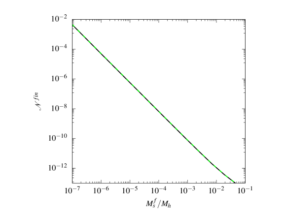
Figure 3: Differential subhalo MF with DF (solid black line) and without (dashed green line) in current purely accreting Milky Way mass haloes (with virial mass $M_{\rm h}=2.2\times 10^{12}$ M_⊙).
(A colour version of this Figure is available in the online journal.)

And dividing the radial abundance and MF of subhaloes with mass $M_{\rm s}^{\rm f}$ (eqs. [43] and [44]) by $4\pi(r^{\rm f})^{2}$ and $4\pi R_{\rm h}^{3}$, respectively, we obtained the number density profile of subhaloes of mass $M_{\rm s}$, $n^{\rm fin}(r^{\rm f},M_{\rm s}^{\rm f})$, scaled to its total number density $n^{\rm fin}(M_{\rm s}^{\rm f})$. The result in terms of the homologous quantity with no DF (denoted as usual by index ‘stp’) is

$$\frac{n^{\rm fin}(r^{\rm f},M_{\rm s}^{\rm f})}{n^{\rm fin}(M_{\rm s}^{\rm f})}\!\approx\!\frac{n^{\rm stp}(r^{\rm f},M_{\rm s}^{\rm f})}{n^{\rm stp}(M_{\rm s}^{\rm f})}\!\left\{1\!+\!\left[\omega(r^{\rm f})-\bar{\omega}\right]M_{\rm s}\right\}\!.$$ (45)

Again, the scaled subhalo number density profile is equal to its counterpart in the absence of DF, independent of subhalo mass, plus a term proportional to $M_{\rm s}^{\rm f}$ with proportionality factor $\omega(r^{\rm f})-\bar{\omega}$. Since $\omega(r^{\rm f})$ decreases with increasing radius, the factor $\omega(r^{\rm f})-\bar{\omega}$ starts being positive at small radii and ends up being negative at larger ones.

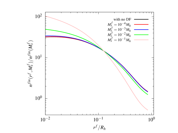
Figure 4: Scaled number density profile of subhaloes of several masses in current purely accreting Milky Way mass haloes. As expected, the number density profiles of subhaloes with $M_{\rm s}^{\rm f}\la 10^{-4}M_{\rm h}$ overlap with the mass-independent profile found in Paper II neglecting DF.
(A colour version of this Figure is available in the online journal.)

In Figure 4 we show the predicted scaled subhalo number density for subhaloes of several masses. We see that the profiles of subhaloes with $M_{\rm s}^{\rm f}\la 10^{-4}M_{\rm h}$ overlap with each other and with the mass-independent subhalo number density profile obtained in Paper II with no DF. However, the profile becomes increasingly steeper for more massive subhaloes. Contrarily to what happens with the subhalo MF, the effect of DF on the subhalo number density profile is notable for subhaloes with $M_{\rm s}^{\rm f}\ga 0.05M_{\rm h}$. This behaviour recovers and explains what is found in simulations (see, e.g., Han et al. 2018).

3.2 Ordinary Haloes

But real haloes alternate accretion periods with major mergers and, even though all halo properties arising from gravitational collapse and virialisation do not depend on their past aggregation history (Salvador-Solé & Manrique, 2021), those arising from tidal stripping and shock-heating and DF do. As a consequence, the properties of halo substructure depend in this case not only on their mass $M_{\rm h}$ and time $t_{\rm h}$, but also on their formation time $t_{\rm f}$, defined, like in previous Papers, as the time they suffered the last major merger. Fortunately, as shown in Paper III, the properties of substructure in ordinary haloes can be derived from those in idealised purely accreting ones. Below, we focus on these properties averaged over the formation time of halos (see the motivation in Paper III) and indicate how to calculate those of haloes formed in specific time intervals. To distinguish the properties of purely accreting haloes from those of ordinary ones the former, derived in Section 3.1, are hereafter denoted with index PA.

When a halo undergoes a major merger, it virialises through violent relaxation and its content is scrambled. After that, it begins to accrete again and to grow inside-out. As a consequence, the mean fraction of accreted subhaloes with $M_{\rm s}^{\rm f}$ at $r^{\rm f}$ in ordinary haloes with $M_{\rm h}$ at $t_{\rm h}$ that are stripped is (Paper III)

$${\mu_{\rm DF}}{}_{\rm[M_{\rm h},t_{\rm h}]}(r^{\rm f},M_{\rm s}^{\rm f})=\int_{0}^{t(r^{\rm f})}{\rm d}t\,n(t)\,\mu_{\rm DF}^{\rm PA}{}_{\rm[M_{\rm h},t_{\rm h}]}(r^{\rm f},M_{\rm s}^{\rm f})~~~$$

$$+\int_{t(r^{\rm f})}^{t_{\rm h}}{\rm d}t\,n(t)\,\bar{\mu}_{\rm DF}{}_{\rm[M(t),t]}(1,M_{\rm s}^{\rm f}),~~~$$ (46)

with a bar on a function of $r^{\rm f}$ denoting the average of that function over all subhaloes out to the scaled radius $r^{\rm f}$. In equation (46), $n(t)$ is the formation time probability distribution function (PDF) of haloes with $M_{\rm h}$ at $t_{\rm h}$ calculated by Manrique et al. (1998) using CUSP (see Raig et al. 2001 for a practical approximation). Since $\mu_{\rm DF}$ of haloes with $M(t)$ at $t$ depends on these two quantities, we write it with subindex [M(t),t]. Consequently, the integral over $t$ in the first term on the right of equation (46) can be rewritten as $\mu^{\rm PA}_{\rm DF}{}_{\rm[M_{\rm h},t_{\rm h}]}(r^{\rm f},M_{\rm s}^{\rm f})\,n^{\rm c}(r^{\rm f})$, where $n^{\rm c}(r^{\rm f})$ is the cumulative formation time PDF of haloes with $M_{\rm h}$ at $t_{\rm h}$ up to the time $t(r^{\rm f})$ when they reached radius $r^{\rm f}$ and mass $M(r^{\rm f})$.

As shown in Paper III, the relation (46) can be used to obtain $\bar{\mu}_{\rm DF}$ from the homologous function $\mu_{\rm DF}^{\rm PA}$ derived in Section 3.1. To do this we must first multiply it by ${\cal N}^{\rm acc}(r^{\rm f},M_{\rm s}^{\rm f})$ and integrate over $r^{\rm f}$ out to $R_{\rm h}$. The result is

$$\bar{\mu}_{\rm DF}{}_{\rm[M_{\rm h},t_{\rm h}]}(R_{\rm h},M_{\rm s}^{\rm f})=\overline{\mu_{\rm DF}^{\rm PA}{}_{\rm[M_{\rm h},t_{\rm h}]}\,n^{\rm c}}(R_{\rm h},M_{\rm s}^{\rm f})~~~~~~~~~~~~~~~$$

$$\!+\!\!\int_{0}^{t_{\rm h}}\!\!{\rm d}t\,n(t)\,\bar{\mu}_{\rm DF}{}_{\rm[M(t),t]}(R_{\rm h},M_{\rm s}^{\rm f})\frac{M(t)}{M_{\rm h}},~~$$ (47)

where the first term on the right is related to its counterpart with no DF (eq. [41]) through

$$\overline{{\mu_{\rm DF}^{\rm PA}}_{\rm[M_{\rm h},t_{\rm h}]}n^{\rm c}}(r^{\rm f},M_{\rm s}^{\rm f})\approx\overline{{\mu^{\rm PA}}_{\rm[M_{\rm h},t_{\rm h}]}n^{\rm c}}(r^{\rm f})\left[1+\widetilde{\omega}(r^{\rm f})M_{\rm s}^{\rm f}\right]~$$ (48)

$$\widetilde{\omega}(r^{\rm f})\equiv\frac{\overline{\omega^{\rm PA}\mu^{\rm PA}_{\rm[M_{\rm h},t_{\rm h}]}n^{\rm c}}(r^{\rm f})}{\overline{\mu^{\rm PA}_{\rm[M_{\rm h},t_{\rm h}]}n^{\rm c}}(r^{\rm f})}.~~~~~~~~~~~~~~~~~~~~~~~~~~~~~~~~~~~~~$$ (49)

Solving the Volterra equation of second kind (47) for $\bar{\mu}_{\rm DF}{}_{\rm[M(t),t]}(R_{\rm h},M_{\rm s}^{\rm f})$ as a function of $t$, plugging the solution in the integral on the right of equation (46) and taking into account the analogous expression for the case with no DF, we arrive at

$${\mu_{\rm DF}}{}_{\rm[M_{\rm h},t_{\rm h}]}(r^{\rm f},M_{\rm s}^{\rm f})\approx{\mu}_{\rm[M_{\rm h},t_{\rm h}]}(r^{\rm f})\left[1+\omega(r^{\rm f})M_{\rm s}^{\rm f}\right]~~~~~~~~~~$$ (50)

$$\omega(r^{\rm f})\!\equiv\!\frac{\omega^{\rm PA}\!\mu^{\rm PA}_{\rm[M_{\rm h},t_{\rm h}]}\!n^{\rm c}(r^{\rm f})}{{\mu}_{\rm[M_{\rm h},t_{\rm h}]}(r^{\rm f})}\,~~~~~~~~~~~~~~~~~~~~~~~~~~~~~~~~~~~~~~~$$

$$+\frac{\int_{t(r^{\rm f})}^{t_{\rm h}}\!{\rm d}t\,n(t)\,\overline{{\mu_{\rm DF}}_{\rm[M(t),t]}\!-\!\mu_{\rm[M(t),t]}}(1,M_{\rm s}^{\rm f})/M_{\rm s}^{\rm f}}{{\mu}_{\rm[M_{\rm h},t_{\rm h}]}(r^{\rm f})}.~~$$ (51)

To write equation (51) we have taken into account that, according to equation (47) and the form of the function $\mu{}_{\rm[M(t),t]}(r^{\rm f},M_{\rm s}^{\rm f})$ for ordinary haloes with no DF calculated in Paper III, $\overline{{\mu_{\rm DF}}_{\rm[M(t),t]}\!-\!\mu_{\rm[M(t),t]}}(R_{\rm h},M_{\rm s}^{\rm f})$ is proportional to $M_{\rm s}^{\rm f}$, so $\omega$ is a function of $r^{\rm f}$ alone. We thus see that the typical value of $\mu_{\rm DF}$ of ordinary halos with $M_{\rm h}$ at $t_{\rm h}$ is identical to that of purely accreting halos (eq. [41]), but with a different function $\omega(r^{\rm f})$, related to its counterpart $\omega^{\rm PA}(r^{\rm f})$ in pure accretion through equation (51).

Having determined $\mu_{\rm DF}{}_{\rm[M_{\rm h},t_{\rm h}]}(r^{\rm f},M_{\rm s}^{\rm f})$, we must simply plug it into equation (39) in order to obtain the radial abundance of subhaloes with $M_{\rm s}^{\rm f}$. Then, integrating the latter over $r^{\rm f}$, we are led to the subhalo MF in ordinary haloes with DF. Of course, since the subhalo in of purely accreting halos was identical to that found without DF, so will also be the subhalo MF of ordinary halos derived from it. And the same procedure above will lead to the scaled subhalo number density profile of ordinary haloes with DF. Since that in purely accreting haloes depends on subhalo mass, the same reasoning as for the subhalo MF suggests that the scaled number density profile with DF should also depend on subhalo mass and be slightly steeper for more massive subhaloes. However, as shown in Figure 5, this effect is insignificant now. The reason for this is that the average over the formation time of haloes gives more weight to large times (see the factor $M(t)/M_{\rm h}$ in the second term on the right of eq. [47]) where the only non-scrambled subhaloes are recent arrivals with little time to suffer significant DF.

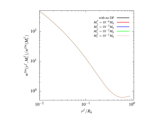
Figure 5: Same as Figure 4 but for ordinary haloes averaged over their formation time. All curves overlap at the scale of the Figure.
(A colour version of this Figure is available in the online journal.)

We thus see that DF has a negligible effect on the subhalo MF and radial distribution of ordinary haloes when averaged over their halo formation times. But that is not true, of course, for haloes formed in specific time intervals. To obtain the latter we should apply the same procedure above, but using the formation time PDF, $n(t)$, multiplied by the suited top-hat window defining the desired formation time interval (see Paper III). Then, the effects of DF would be substantially more marked for haloes formed long time ago where DF would have more time to proceed. Specifically, the earlier haloes would form, the closer their properties would be to those of purely accreting haloes. It is thus unsurprising that, in the MW-mass halo A in the Level 1 Aquarius simulation analysed by Han et al. (2016), substrucure was well described by our results for purely accreting haloes (Paper II), except for the radial distribution of massive subhaloes, which are better described by the results derived in Section 3.1.

4 Summary and Concluding Remarks

With this Paper we culminate a detailed comprehensive study of halo substructure. This has been accomplished in a fully analytic manner in the peak model of structure formation (with no free parameter) together with a realistic model of subhalo tidal stripping and shock-heating (with only two parameters tuned by means of numerical experiments).

In Paper I we derived the properties of unevolved subhaloes falling into purely accreting haloes, using the statistics of nested peaks. In Paper II we studied their tidal stripping and shock-heating within the host haloes. And in Paper III we extended the analysis to ordinary haloes of all masses and formation times. The theoretical properties obtained accurately reproduced those found in cosmological $N$-body simulations and explained them. However, to facilitate the analytic treatment we neglected the effects of DF, so the results held for low-mass subhaloes only.

In the present Paper, we have remedied that limitation by incorporating DF, taking into accounts its crossed effects with tidal stripping and shock-heating of subhaloes. After monitoring the multiple concatenated orbits of individual subhaloes at accretion and finding their final mass and radius at the time haloes are observed, we have studied the effects of DF on their global subhalo population in both purely accreting haloes and real ones having alternated periods of smooth accretion with major mergers.

In spite of the complexity and entanglement of the different mechanisms driving the properties of halo substructure, we have found simple non-parametric expressions for the subhalo MF and number density profile showing how DF alters the results obtained in previous Papers taking only into account tidal stripping and shock-heating. These expressions reproduce and explain the results of high-resolution $N$-body simulations and allow one to extend them to haloes of any mass $M_{\rm h}$, redshift $z$ and formation time $t$ in any desired CDM cosmology. We have found that the effects of DF go unnoticed in the subhalo MF and are only significant in the radial distribution of massive subhaloes ($M_{\rm s}>10^{-4}M_{\rm h}$) in haloes having formed early enough.

To conclude we want to mention some possible applications of the present work. Given the correlation between galaxy stellar mass and the mass of their subhalo hosts, the results given here open the possibility to determine the galaxy bias directly from peak statistics without the need to model the halo occupation distribution of galaxies. With small modifications, the present analytic treatment of DF could also be applied to the modelling of other self-gravitating systems.

DATA AVAILABILITY

The data underlying this article will be shared on reasonable request to the corresponding author.

ACKNOWLEDGEMENTS

This work was funded by the Spanish MCIN/AEI/10.13039/ 501100011033 through grants CEX2019-000918-M (Unidad de Excelencia ‘María de Maeztu’, ICCUB) and PID2022-140871NB-C22 (co-funded by FEDER funds) and by the Catalan DEC through the grant 2021SGR00679.

Appendix A Relative Energy and Angular momentum Increments

To leading order in the effects of DF, Equation (6) implies

$$\frac{\Delta L}{L}=-A_{\rm L}(k,r,M_{\rm s})T(k,r,M_{\rm s}),$$ (52)

where $T(k,r,M_{\rm s})$ is the orbital period with DF, equal, to leading order, to that with no DF. On the other hand, equation (4) states that $\Delta E$ is $-A_{\rm E}$ times the action of the mechanical system, for slowly varying $E$, is an adiabatic invariant, so it is equal to the value found in the absence of DF. Consequently, equation (4) implies

$$\frac{\Delta E}{E}=P(k,r)A_{\rm E}(k,r,M_{\rm s})T(k,r,M_{\rm s}),$$ (53)

where

$$P(k,r)\equiv\frac{-2r}{kGM(r)S(k,r)}\frac{\int_{0}^{T}{\rm d}tv^{2}(t)}{\int_{0}^{T}dt}=\frac{-2r}{kGM(r)S(k,r)}\frac{\int_{r_{\rm per}}^{r}{\rm d}x\frac{v^{2}(x,k,r)}{v_{\rm r}(x,k,r)}}{\int_{r_{\rm per}}^{r}{\rm d}x\frac{1}{v_{\rm r}(x,k,r)}},$$ (54)

with the second equality on the right holding to leading order in the effects of DF, where

$$v^{2}(x,k,r)=2[\Phi(r)-\Phi(x)]+k\frac{GM(r)}{r}~~~~~~~~~~~~~~~{\rm and}~~~~~~~~~~~~~~~~~v^{2}_{\rm r}(x,k,r)=2[\Phi(r)-\Phi(x)]+k\frac{GM(r)}{r}\left[1-\left(\frac{r}{x}\right)^{2}\right]$$ (55)

(with $0<(v-v_{\rm r})/v<1$) are the 3D velocity and its radial component, respectively, at radii $x$ over the orbit without DF of subhaloes with $k$ and $r$ and $r_{\rm per}/r\equiv\tilde{k}\approx k(1+\sqrt{1+8/k})/4$.

The functions $PA_{\rm E}T$ and $A_{\rm L}T$ determining $\Delta E/E$ and $\Delta L/L$ (eqs. [53] and [52]) can be calculated, to leading order, from equations (4) and (6), with $A$ given by equation (2), over orbits without DF, i.e. using $v$ and $v_{\rm r}$ given by equations (55). The result is

$$\frac{\Delta E}{E}=P(k,r)A_{\rm E}(k,r,M_{\rm s})T(k,r,M_{\rm s})=30.86\,\pi G^{2}Q\frac{M_{\rm s}}{M_{\rm h}}\,\frac{-2r}{kGM(r)S(k,r)}\int_{r_{\rm per}}^{r}{\rm d}x\,x^{-1.875}f_{\rm dDM}(x)\frac{v^{2}(x,k,r)}{v_{\rm r}(x,k,r)}H(x,k,r)$$ (56)

$$\frac{\Delta L}{L}=-A_{\rm L}(k,r,M_{\rm s})T(k,r,M_{\rm s})=-30.86\,\pi G^{2}Q\frac{M_{\rm s}}{M_{\rm h}}\int_{r_{\rm per}}^{r}{\rm d}x\,x^{-1.875}f_{\rm dDM}(x)\frac{1}{v_{\rm r}(x,k,r)}H(x,k,r),$$ (57)

where $H(x,k,r)\equiv[{\rm erf}(X)-\sqrt{2}/\pi X\exp(-X^{2})]/X^{3}$, with $X\equiv\sqrt{3/2}\,v(x,k,r)/\sigma(x)$. To write equations (56) and (57) we have used the universal dDM fraction $f_{\rm dDM}(r)$ (Papers II and III) and the pseudo phase-space density $\rho(r)/\sigma^{3}(r)=Q/M_{\rm h}\,r^{-1.875}$, with $Q=9.56\times 10^{17}$ (M_⊙/Mpc³) (km/s)^-3 (Taylor & Navarro 2001; Salvador-Solé & Manrique 2021 and references therein). The case $k=1$ ($r_{\rm per}=r$) is excluded from expressions (56) and (57). But this is not a problem because this corresponds to the extreme value of $k$ for accreted subhaloes (Paper II).

These values of $\Delta E/E$ and $\Delta L/L$ can be calculated with no need to previously determine the subhalo orbits with DF. However, they still involve two numerical integrals. To get a purely analytic treatment we can split those integrals in two parts and Taylor expand to first order the integrants around the lower and upper radii, which allows us to carry out the integrals analytically. The separation radius $r_{\rm c}$ is taken such that the approximate values of $v_{\rm r}$, the most sensitive quantity (it is a first order term at the denominator of the integrants; see below), coincide at that matching radius of both parts. This leads to $r_{\rm c}(k,r)/r_{\rm per}-1$ equal to the solution of the quadratic equation $Ax^{2}+Bx+C=0$, with

$$A=q_{u}(k,r)[\tilde{k}^{4}\!-\!q_{l}(k.r)],~~B=1-\frac{q_{l}(k,r)}{k}+\tilde{k}^{3}\left[\frac{1}{k}\!-\!1\!-\!2(1\!-\!\tilde{k})q_{u}(k,r)\right]~~{\rm and}~~C=-\tilde{k}^{2}(1\!-\!\tilde{k})\left[\frac{1}{k}\!-\!1\!-(1\!-\!\tilde{k})\!q_{u}(k,r)\right],$$

being $q_{u}(k,r)\equiv({\rm d}\ln M/{\rm d}\ln r-2)/k+3$ and $q_{l}(k,r)\equiv\tilde{k}M(\tilde{k}r)/M(r)$. We remark that $q_{u}(k,r)$ and $q_{l}(k,r)$ are weakly dependent on $r$ and so is also $\tilde{k}_{\rm c}=r_{\rm c}/r_{\rm per}$.

In the upper radial parts, we have (see eqs. [55])

$$v^{2}(x,k,r)\approx k\frac{GM(r)}{r}\left[1-\frac{2}{k}\left(\frac{x}{r}-1\right)\right],\quad\quad~v^{2}_{\rm r}(x,k,r)\approx 2v^{2}(x,k,r)\left(1-\frac{x}{r}\right)\left[\frac{1}{k}-1+\left\{2+\frac{{\rm d}\ln[M(r)/r^{2}]}{{\rm d}\ln r}\right\}\left(\frac{x}{r}-1\right)\right],~$$ (58)

$$f_{\rm dDM}(x)\approx f_{\rm dDM}(r)\left[1+\frac{{\rm d}\ln f_{\rm dDM}}{{\rm d}\ln r}\left(\frac{x}{r}-1\right)\right]~~~~~~~~~~~~~~~~~~~~~~~~~~~~~~~~~~~~~~~~~~~~~~~~~~~~~~~~~~~~~~~~~~~~~~~~~~~~~~~~~~~~~~~~~~~~~~~~~~~~~~$$ (59)

and, given the isotropic Jeans equation and the form of $\rho(r)/\sigma^{3}(r)$,

$$\frac{2\sigma^{2}(x)}{3v^{2}(x,k,r)}\frac{{\rm d}\ln\left[\rho^{5/3}(x)\,x^{1.25}\right]}{{\rm d}\ln x}\!=\!-\frac{2GM(x)}{xv^{2}(x,k,r)}\!\approx\!\frac{-1}{k/2-(x/r-1)}\left\{1+\frac{{\rm d}\ln[M(r)/r]}{{\rm d}\ln r}\left(\frac{x}{r}-1\right)\right\},$$ (60)

(with $\rho(r)\sim r^{-2.5}$ at the radii of interest) implies $3v^{2}(r)/[2\sigma^{2}(r)]\approx 1.46k$,

$$H(x,k,r)\approx H(k)\left[1-\frac{\partial\ln H}{\partial\ln x}\Big|_{r}\left(\frac{x}{r}-1\right)\right],~~~~~~~~~~~~~~~{\rm with}~~~~~~~~~~~~~~~~\frac{\partial\ln H}{\partial\ln x}\Big|_{r}\approx\frac{{\rm d}\ln H(k)}{{\rm d}\ln k}\left[\frac{2}{k}+\frac{{\rm d}\ln M(r)/r}{{\rm d}\ln r}\right]$$ (61)

and $H(k)\equiv(1.46k)^{-3/2}[{\rm erf}(\sqrt{1.46k})-2\sqrt{1.46k/\pi}\,\exp(-1.46k)]$.

In these conditions, the integrals in equations (56) and (57) above $r_{\rm c}$ take the fully analytic form

$$\frac{\Delta E}{E}\bigg|_{u}\!\approx-\frac{2M_{\rm s}I_{0}(r)H(k)}{S(k,r)}\left(\!\frac{1-\tilde{k}}{1\!-\!k}\!\right)^{\!\frac{1}{2}}I_{1}\!\Big[\tilde{k},D(k,r,1)-\frac{2}{k}\Big]~~~~~~~~~~\frac{\Delta L}{L}\bigg|_{u}\!\approx-M_{\rm s}I_{0}(r)H(k)\left(\!\frac{1-\tilde{k}}{1-k}\!\right)^{\!\frac{1}{2}}I_{1}\!\left[\tilde{k},D(k,r,1)\right],~$$ (62)

where

$$I_{0}(r)\equiv 43.64\pi G^{2}f_{\rm dDM}(r)\frac{\rho(r)}{\sigma^{3}(r)}r\left[\frac{GM(r)}{r}\right]^{-{1/2}}~~~~~~~~~~~~~~I_{1}(\tilde{k},D)\equiv 1+0.625(1-\tilde{k})\left\{1-\left[\frac{1}{1.875}+\frac{3(1+\tilde{k})}{5}\right]D\right\},~~~~~~~~~~~~~~~~~$$

$${\rm with}~D(k,r,q)\equiv\frac{{\rm d}\ln f_{\rm dDM}}{{\rm d}\ln r}-\frac{\partial\ln H}{\partial\ln x}\Big|_{r}-\!\frac{q}{2(q-k)}\frac{{\rm d}\ln[M(r)/r^{2-3k}]}{{\rm d}\ln r},~{\rm so}~I_{1}(\tilde{k},D)~{\rm is~weakly~dependent~on~}r~{\rm provided~}q~{\rm is}.\,~~~~~~~~~~~~~$$

And proceeding in a similar way, the integrals in the lower radial parts lead to

$$\frac{\Delta E}{E}\bigg|_{l}\!\approx-\frac{2M_{\rm s}I_{0}(\tilde{k}r)H(k)}{S(k,\tilde{k}r)}\left(\!\frac{1-\tilde{k}_{\rm c}}{q_{l}\!-\!k}\!\right)^{\!\frac{1}{2}}I_{1}\!\Big[\tilde{k}_{\rm c},D(k,\tilde{k}r,q_{l})\!-\!\frac{2}{k}\Big]~~~~~~~~~~\frac{\Delta L}{L}\bigg|_{l}\!\approx-M_{\rm s}I_{0}(\tilde{k}r)H(k)\left(\!\frac{1-\tilde{k}_{\rm c}}{q_{l}\!-\!k}\!\right)^{\!\frac{1}{2}}I_{1}\!\left[\tilde{k}_{\rm c},D(k,\tilde{k}r,q_{l})\right],$$ (63)

where $\tilde{k}_{\rm c}\equiv r_{\rm c}/r_{\rm per}$ is essentially a function of $k$ only, as $\tilde{k}$. Hence, adding up the upper and lower parts of the integrals, we arrive at the desired fully analytic expressions of $\Delta E/E$ and $\Delta L/L$.

Appendix B Evolved-to-Original Apocentric Radius and Mass Ratios

The partial derivatives entering the definition of the function $\mu_{\rm DF}$ (eq. [40]) are part of the Jacobian $J_{r^{\rm f},M_{\rm s}^{\rm f}}^{r,M_{\rm s}}$ of the transformation: $r=r(v,r^{\rm f},M_{\rm s}^{\rm f})$ and $M_{\rm s}=M_{\rm s}(v,r^{\rm f},M_{\rm s}^{\rm f})$, i.e. the inverse of the Jacobian $J_{r,M_{\rm s}}^{r^{\rm f},M_{\rm s}^{\rm f}}$ of the transformation $r^{\rm f}=r^{\rm f}(v,r,M_{\rm s})$ and $M_{\rm s}^{\rm f}=M_{\rm s}^{\rm f}(v,r,M_{\rm s})$ defined in Section 2.2. The latter Jacobian must be calculated recursively, like the functions $r_{i}$ and $M_{i}$ themselves, taking into account that, after the $i+1$ orbit, the Jacobian $J_{r,M_{\rm s}}^{r_{i+1},M_{i+1}}$ is the matrix product of the Jacobian $J_{r,M_{\rm s}}^{r_{i},M_{i}}$ calculated in the previous step times the Jacobian $J_{r_{i},M_{i}}^{r_{i+1},M_{i+1}}$ of the new elementary transformation $r_{i+1}=r_{i+1}(v,r_{i},M_{i})$ and $M_{i+1}=M_{i+1}(v,r_{i},M_{i})$, whose elements follow from the following partial derivatives (see eqs. [16]-[14])

$$\frac{\partial\,r_{i+1}}{\partial\,x_{i}}=\frac{1}{2}\,\frac{\partial\{r_{i}\left[Q^{\rm f}(k_{i},r_{i},M_{i})+Q^{\rm f}(k_{i},r_{i},M_{i+1}\right]\}}{\partial x_{i}}\qquad\qquad\qquad\qquad\qquad\frac{\partial M_{i+1}}{\partial x_{i}}=\frac{\partial\left[M_{i}\frac{f(c_{i}Q_{i+1})}{f(c_{i})}\right]}{\partial x_{i}}$$ (64)

where the function $x_{i}$ stands for any of the two variables: $M_{i}$ and $r_{i}$. Of course, the partial derivative of each quantity with respect to $r_{i}$ is the direct partial with respect to that variable $r_{i}$ plus the partial derivative with respect to $k_{i}$ times the partial of $k_{i}=v^{2}/[v^{2}-2GM(r_{i})/r_{i}]$ with respect to $r_{i}$. On the other hand, as $Q_{i+1}(k_{i},r_{i},M_{i})$ is the solution of the implicit equation (17), its derivatives can be obtained from derivation of that equation, leading to

$$\frac{\partial Q_{i+1}}{\partial x_{i}}=\frac{f(c_{i})Q_{i+1}^{3}\frac{\partial F(k_{i},r_{i},M_{i})}{\partial x_{i}}}{c_{i}\frac{{\rm d}f(c_{i}Q_{i+1})}{{\rm d}(c_{i}Q_{i+1})}-3\frac{f\left(c_{i}Q_{i+1}\right)}{Q_{i+1}}}~~~~~~~~~~~~~~~~~~\qquad\qquad\qquad\qquad F(k_{i},r_{i},M_{i})=\frac{f\left[c(r_{i})\tilde{k}_{i}Q^{\rm f}(k_{i},r_{i},M_{i}/2)\right]}{f[c(r_{i})]\tilde{k}_{i}[Q^{\rm f}(k_{i},r_{i},M_{i}/2)]^{3}}.$$ (65)

(The derivatives ${\rm d}c_{i}/{\rm d}x_{i}$ are null because $c_{i}$ is the initial concentration at the $i+1$ orbit, so it does not vary when the $x_{i}$ values change.)

To leading order in $\Delta E/E$ and $\Delta L/L$, the only non-null elements of the Jacobians $J_{M_{\rm s},r}^{M_{i+1},r_{i+1}}$ found at each step are those in the diagonal, which are precisely equal to the product of the corresponding elements of the two Jacobians that are multiplied. Consequently, the same is true for the final Jacobian $J_{M_{\rm s},r}^{M_{\rm s}^{\rm f},r^{\rm f}}$ whose diagonal elements take, to first order, the form (see eqs. [19]-[21] and [29]-[33])

$$\frac{\partial r^{\rm f}}{\partial r}=\prod_{0}^{\nu}\frac{\partial r_{i+1}}{\partial r_{i}}=\left(\prod_{i=0}^{\nu}\frac{r_{i+1}}{r_{i}}\right)\!\left(1+\sum_{i=0}^{\nu}\frac{\Delta r_{i}}{r_{i}}+\sum_{i=0}^{\nu}r_{i}\frac{\partial}{\partial r_{i}}\frac{\Delta r_{i}}{r_{i}}\right)\approx\frac{r^{\rm f}}{r}\left(1+\frac{{\rm d}\ln I_{0}}{{\rm d}\ln r}\right)\frac{\Delta r}{r}~~~~~~~~~~~~~~~~~~~~~~~~~~~~~~~~~~~~~~~~~~~~~$$ (66)

$$\frac{\partial M_{\rm s}^{\rm f}}{\partial M_{\rm s}}=\prod_{i=0}^{\nu}\!\frac{\partial M_{i+1}}{\partial M_{i}}=\!\Bigg(\prod_{i=0}^{\nu}\!\frac{M_{i+1}^{\prime}}{M_{i}}\Bigg)\Bigg(1+2J(k,r)\sum_{i=0}^{\nu}\frac{\Delta r_{i}}{r_{i}}\Bigg)=\frac{M_{\rm s}^{\rm tr}}{M_{\rm s}}\left[1+2J(k,r)\frac{\Delta r}{r}\right].~~~~~~~~~~~~~~~~~~~~~~~~~~~~~~~~~~~~~~~~~~~~~~~~$$ (67)

To derive equations (66) and (67) we have taken into account equations (7)-(8) with $\Delta E/E$ and $\Delta L/L$ given in Appendix A, which leads to $\partial(\Delta r_{i}/r_{i})/\partial M_{i}=(\Delta r_{i}/r_{i})/M_{i}$ and

$$\frac{\Delta r_{i}}{r_{i}}\!=-\frac{k_{i}H(k_{i})}{1\!-\!k_{i}}M_{i}\left[\!\frac{I_{0}(r_{i})}{S(k_{i},r_{i})}\left(\!\frac{1\!-\!\tilde{k}_{i}}{1\!-\!k_{i}}\!\right)^{\!\frac{1}{2}}\!\!\tilde{I}_{1}\!\left(\tilde{k}_{i}\right)\!+\!\frac{I_{0}(\tilde{k}_{i}r_{i})}{S(k_{i},\tilde{k}_{i}r_{i})}\left(\!\frac{1\!-\!\tilde{k}_{{\rm ci}}}{q_{li}\!-\!k_{i}}\!\right)^{\!\frac{1}{2}}\!\!\tilde{I}_{1}\!\left(\tilde{k}_{{\rm ci}}\right)\!\right],$$ (68)

implying

$$r_{i}\frac{\partial}{\partial r_{i}}\!\frac{\Delta r_{i}}{r_{i}}\approx-\frac{k_{i}H(k_{i})}{1\!-\!k_{i}}M_{i}\!\left[\frac{I_{0}(r_{i})}{S(k_{i},r_{i})}\frac{\partial\ln I_{0}/S}{\partial\ln r_{i}}\left(\!\frac{1\!-\!\tilde{k}_{i}}{1\!-\!k_{i}}\right)^{\!\frac{1}{2}}\!\tilde{I}_{1}(\tilde{k}_{i})+\!\frac{I_{0}(\tilde{k}_{i}r_{i})}{S(k_{i},\tilde{k}_{i}r_{i})}\frac{\partial\ln I_{0}/S}{\partial\ln(\tilde{k}_{i}r_{i})}\left(\!\frac{1\!-\!\tilde{k}_{{\rm ci}}}{q_{l}\!-\!k_{i}}\!\right)^{\!\frac{1}{2}}\!\tilde{I}_{1}(\tilde{k}_{\rm ci})\right]\approx\frac{{\rm d}\ln\tilde{I}_{0}}{{\rm d}\ln r_{i}}\frac{\Delta r_{i}}{r_{i}},$$ (69)

where we have defined $\tilde{I}_{1}(\tilde{k})\equiv 0.625(1-\tilde{k})[1/1.875\!+\!3/5(1-\tilde{k})]2/k$ and $\tilde{I}_{0}(r)\equiv j(r)I_{0}(r)$, with $j(r)\equiv f[c(r)]/\ln[1+c(r)]$ being a weak function of $r$, and we have neglected the logarithmic radial derivative of $(1-\tilde{k})j(r){\rm d}\ln\tilde{I}_{0}/{\rm d}\ln r$ in front of unity.

Equation (69) leads to

$$\frac{\partial}{\partial\ln r}\frac{\Delta r}{r}\approx\frac{{\rm d}\ln\tilde{I}_{0}}{{\rm d}\ln r}\frac{\Delta r}{r},\!$$ (70)

whose solution is

$$\frac{\Delta r}{r}\approx-Y(k)\tilde{I}_{0}(r)M_{\rm s}\qquad~~~~~~~~~~~~~~~~~~~~~~~~~\qquad Y(k)=\frac{k^{2}H(k)}{2(1\!-\!k)}\left[\left(\!\frac{1\!-\!\tilde{k}}{1\!-\!k}\!\right)^{\!\frac{1}{2}}\!\!\tilde{I}_{1}\!\left(\tilde{k}\right)\!+\!(k-0.1)\left(\!\frac{1\!-\!\tilde{k}_{{\rm c}}}{q_{l}\!-\!k}\!\right)^{\!\frac{1}{2}}\!\!\tilde{I}_{1}\!\left(\tilde{k}_{{\rm c}}\right)\!\right].$$ (71)

Then, equation (67) implies

$$\frac{\partial M_{\rm s}}{\partial M_{\rm s}^{\rm f}}=\frac{M_{\rm s}}{M_{\rm s}^{\rm tr}}\left[1-2J(k,r)\frac{\Delta r}{r}\right]\approx Y(k)\frac{\partial M_{\rm s}}{\partial M_{\rm s}^{\rm tr}}\left[1+2J(k,r)\tilde{I}_{0}(r)M_{\rm s}\right].$$ (72)

And differentiating $M(r^{\rm f})$ with respect to $M(r)$ in the Taylor expansion

$$M(r^{\rm f})=M(r)\left[1+\frac{{\rm d}\ln M}{{\rm d}\ln r}\frac{\Delta r}{r}\right]\approx M(r)\left[1-Y(k)\frac{{\rm d}\ln M}{{\rm d}\ln r}\tilde{I}_{0}(r)M_{\rm s}\right]$$ (73)

and neglecting the double logarithmic derivative of $M(r)$, we obtain, to first order,

$$\frac{\partial M(r)}{\partial M(r^{\rm f})}\approx 1+Y(k)\frac{{\rm d}\ln(M\tilde{I}_{0})}{{\rm d}\ln r^{\rm f}}\tilde{I}_{0}(r^{\rm f})M_{\rm s}^{\rm f}.$$ (74)

Equations (72) and (74) give the two factors in the first term of the angular bracket in $\mu_{\rm DF}$ (eq. [40]), while the factors in the second term are null. Consequently, taking into account the expression of $\mu$ (eq. [37]) and the relation (30), equation (40) can be expressed, to first order, in the form

$$\mu_{\rm DF}(r^{\rm f},M_{\rm s}^{\rm f})\approx\mu(r^{\rm f})+\kappa(r^{\rm f})\frac{{\rm d}\ln(M\tilde{I}_{0})}{{\rm d}\ln r^{\rm f}}\tilde{I}_{0}(r^{\rm f})M_{\rm s}^{\rm f},$$ (75)

where $\kappa(r^{\rm f})\equiv\langle YM_{\rm s}^{\rm tr}/M_{\rm s}\rangle(r^{\rm f})$ and $\mu(r^{\rm f})\equiv\langle M_{\rm s}^{\rm tr}/M_{\rm s}\rangle(r^{\rm f})$ (eq. [37]). Note that, since the $v$-PDF is tiny near its upper bound (see Paper II), the upper limit of the integral over $v$ defining the average in angular brackets, equal to first order to

$$v_{\rm max}=\left[\frac{GM(r^{\rm f})}{r^{\rm f}}\right]^{1/2}\left\{1+\frac{1}{2}\frac{{\rm d}\ln[M(r^{\rm f})/r^{\rm f}]}{{\rm d}\ln r^{\rm f}}\frac{\Delta r}{r}(r^{\rm f},M_{\rm s}^{\rm f})\right\},$$ (76)

can be approximated by $[GM(r^{\rm f})/r^{\rm f}]^{1/2}$, so angular brackets in equation (40) can be seen to denote velocity average for subhaloes at $r^{\rm f}$, as it does in equation (37) for subhaloes at $r$.

References

- Angulo et al. (2009) Angulo R. E., Lacey C. G., Baugh C. M., Frenk C. S., 2009, MNRAS, 399, 983
- Arena & Bertin (2007) Arena S. E., Bertin G. 2007, A&A, 463, 921
- Bhattacharyya & Singh Bagla (2023) Bhattacharyya D., Singh Bagla J., 2023, arXiv, arXiv:2308.05598
- Bekenstein (1989) Bekenstein J. D., 1989, International Journal of Theoretical Physics, 28, 967
- Benson et al. (2002) Benson, A. J., Lacey, C. G., Baugh C. M., Cole S., Frenk C. S., 2002, MNRAS, 333, 156
- Benson et al. (2013) Benson A. J., Farahi A., Cole S., et al., 2013, MNRAS, 428, 1774
- Berezhiani et al. (2023) Berezhiani L., Cintia G., De Luca V., Khoury J., 2023, arXiv, arXiv:2311.07672
- Binney & Tremaine (2008) Binney J. & Tremaine S., 2008, Galactic Dynamics: Second Edition
- Borukhovetskaya et al. (2022) Borukhovetskaya A., Errani R., Navarro J. F., Fattahi A., Santos-Santos I., 2022, MNRAS, 509, 5330
- Bose et al. (2016) Bose S., Hellwing W. A., Frenk C. S., Jenkins A., Lovell M. R., Helly J. C., Li B., 2016, MNRAS, 455, 318
- Bose et al. (2020) Bose S., Deason A. J., Belokurov V., Frenk C. S., 2020, MNRAS, 495, 743
- Boylan-Kolchin et al. (2010) Boylan-Kolchin M., Springel V., White S. D. M., Jenkins A., 2010, MNRAS, 406, 896
- Buehler & Desjacques (2023) Buehler R., Desjacques V., 2023, PhRvD, 107, 023516
- Cautun et al. (2014a) Cautun M., Frenk C. S., van de Weygaert R., Hellwing W. A., Jones B. J. T., 2014a, MNRAS, 445, 2049
- Cautun et al. (2014b) Cautun M., Hellwing W. A., van de Weygaert R., Frenk C. S., Jones B. J. T., Sawala W., 2014b, MNRAS, 445, 2049
- Chandrasekhar (1943) Chandrasekhar S., 1943, ApJ, 97, 255
- Chiba (2023) Chiba R., 2023, MNRAS, 525, 3576. doi:10.1093/mnras/stad2324
- Choi et al. (09) Choi J.-H., Weinberg M. D., Katz N., 2009, MNRAS, 400, 1247
- Colpi et al. (1999) Colpi M., Mayer L., Governato F., 1999, ApJ, 525, 720
- Colpi & Pallavicini (1998) Colpi M. & Pallavicini A., 1998, ApJ, 502, 150
- Cunningham et al. (2020) Cunningham E. C., Garavito-Camargo N., Deason A. J., et al., 2020, ApJ, 898, 4
- DeGraf et al. (2023) DeGraf C., Chen N., Ni Y., Di Matteo T., Bird S., Tremmel M., Croft R., 2023, MNRAS.tmp
- Dekel et al. (2021) Dekel A., Freundlich J., Jiang F., Lapiner S., Burkert A., Ceverino D., Du X., et al., 2021, MNRAS.tmp
- Diemand et al. (2007) Diemand J., Kuhlen M., Madau P., 2007, ApJ, 657, 267
- Elahi et al. (2009) Elahi P. J., Widrow L. M., Thacker R. J., 2009, Ph. Rev. D, 80, 123513
- Font et al. (2020) Font A. S., McCarthy I. G., Poole-Mckenzie R., Stafford S. G., Brown S. T., Schaye J., Crain R. A., et al., 2020, MNRAS, 498, 1765
- Font, McCarthy, & Belokurov (2020) Font A. S., McCarthy I. G., Belokurov V., 2020, arXiv, arXiv:2011.12974
- Fujita et al. (2002) Fujita Y., Sarazin C. L., Nagashima M., Yano T., 2002, ApJ, 577, 11
- Gan et al. (2010) Gan J., Kang X., Bosch F. C. v. d., Hou J., 2010, MNRAS, 408, 2021
- Gao et al. (2008) Gao L., Navarro J. F., Cole S., Frenk C. S., White S. D. M., Springel V., Jenkins A., Neto A. F., 2008, MNRAS, 387, 536
- Gao et al. (2011) Gao L., Frenk C. S., Boylan-Kolchin M., Jenkins A., Springel V., White S. D. M., 2011, MNRAS, 410, 2309
- Gao et al. (2012) Gao L., Frenk C. S., Jenkins A., Springel V., White S. D. M., 2012, MNRAS, 419, 1721
- Garavitoi-Camargo et al. (2019) Garavito-Camargo N., Besla G., Laporte C. F. P., et al., 2019, ApJ, 884, 51
- Giocoli et al. (2008) Giocoli C., Tormen G., van den Bosch F. C., 2008, MNRAS, 386, 2135
- Giocoli et al. (2010) Giocoli C., Tormen G., Sheth R. K., van den Bosch F. C., 2010, MNRAS, 404, 502
- Green & van den Bosch (2019) Green S. B., van den Bosch F. C., 2019, MNRAS, 490, 2091
- Griffen et al. (2016) Griffen B. F., Ji A. P., Dooley G. A., Gómez F. A., Vogelsberger M., O’Shea B. W., Frebel A., 2016, ApJ, 818, 10
- Han et al. (2016) Han J., Cole S., Frenk C. S., Jing Y., 2016, MNRAS, 457, 1208
- Han et al. (2018) Han J., Cole S., Frenk C. S., Benitez-Llambay A., Helly J., 2018, MNRAS, 474, 604
- Hansen et al. (2006) Hansen S. H., Moore B., Zemp M., & Stadel, J., 2006, JCAP, 1, 014
- Hellwing et al. (2016) Hellwing W. A., Frenk C. S., Cautun M., Bose S., Helly J., Jenkins A., Sawala T., et al., 2016, MNRAS, 457, 3492
- Henry (2000) Henry, J. P., 2000, ApJ, 534, 565
- Ishiyama et al. (2020) Ishiyama T., Prada F., Klypin A. A., Sinha M., Metcalf R. B., Jullo E., Altieri B., et al., 2020, arXiv, arXiv:2007.14720
- Jiang & van den Bosch (2016) Jiang F. & van den Bosch F. C. 2016, MNRAS, 458, 2848
- Jiang et al. (2015) Jiang L., Cole S., Sawala T., Frenk C. S., 2015, MNRAS, 448, 1674
- Jiang et al. (2021) Jiang F., Dekel A., Freundlich J., van den Bosch F. C., Green S. B., Hopkins P. F., Benson A., et al., 2021, MNRAS, 502, 621
- Kampakoglou & Benson (2007) Kampakoglou M. & Benson A. J., 2007, MNRAS, 374, 775
- Klypin et al. (2011) Klypin A. A., Trujillo-Gomez S., Primack J., 2011, ApJ, 740, 102
- Komatsu et al. (2011) Komatsu E., Smith K. M., Dunkley J., Bennet C. L., Gold B., Hinshaw G., Jarosik N., et al. others, 2011, ApJS, 192, 18
- Lacey & Cole (1993) Lacey C. & Cole S., 1993, MNRAS, 262, 627
- Lee (2004) Lee J., 2004, ApJ, 604, L73
- Li et al. (2021) Li H., Vogelsberger M., Bryan G. L., Marinacci F., Sales L. V., Torrey P., 2021
- Lovell et al. (2014) Lovell M. R., Frenk C. S., Eke V. R., et al., 2014, MNRAS, 439, 300
- Ma et al. (2021) Ma L., Hopkins P. F., Ma X., Anglés-Alcázar D., Faucher-Giguère C.-A., Kelley L. Z., 2021, MNRAS.tmp.
- Manrique & Salvador-Solé (1995) Manrique A. & Salvador-Solé E., 1995, ApJ, 453, 6
- Manrique & Salvador-Solé (1996) Manrique A. & Salvador-Solé E., 1996, ApJ, 467, 504
- Manrique et al. (1998) Manrique A., Raig A., Solanes J. M., González-Casado G., Stein, P., Salvador-Solé E., 1998, ApJ, 499, 548
- Mulder (1983) Mulder, W. A. 1983, A&A, 117, 9
- Navarro, Frenk & White (1995) Navarro J. F., Frenk C. S, White S. D. M., 1995, ApJ, 275, 720
- Ogiya & Burkert (2016) Ogiya G. & Burkert A., 2016, MNRAS, 457, 2164
- Oguri & Lee (2004) Oguri M. & Lee J. 2004, MNRAS, 355, 120
- Onions et al. (2012) Onions J., Knebe A., Pearce F. R., Muldrew S. I., Lux H., Knollmann S. R., Ascasibar Y., et al., 2012, MNRAS, 423, 1200
- Peñarrubia et al. (2010) Peñarrubia J., Benson A. J., Walker M. G., Gilmore G., McConnachie A.W., Mayer L., 2010, MNRAS, 406, 1290
- Peñarrubia & Benson (2005) Peñarrubia J. & Benson A. J., 2005, MNRAS, 364, 977
- Peñarrubia et al. (2004) Peñarrubia J., Just A., Kroupa P. 2004, MNRAS, 349, 747
- Pullen et al. (2014) Pullen A. R., Benson A. J., Moustakas L. A., 2014, ApJ, 792, 24
- Raig et al. (2001) Raig, A., González-Casado, G., Salvador-Solé, E. 2001, MNRAS, 327, 939
- Raveh et al. (2021) Raveh Y., Ginat Y. B., Perets H. B., Woods T. E., 2021, MNRAS, 505, 3944
- Rawlings et al. (2023) Rawlings A., Mannerkoski M., Johansson P. H., Naab T., 2023, MNRAS, 526, 2688
- Read et al. (2006) Read J. I., Goerdt T., Moore B., Pontzen A. P., Stadel J., Lake G., 2006, MNRAS, 373, 1451
- Richings et al. (2020) Richings J., Frenk C., Jenkins A., Robertson A., Fattahi A., Grand R. J. J., Navarro J., et al., 2020, MNRAS, 492, 5780
- Salvador-Solé et al. (2012a) Salvador-Solé E., Viñas J., Manrique A., Serra S., 2012a, MNRAS, 423, 2190
- Salvador-Solé et al. (2023) Salvador-Solé E., Manrique A., Canales D., Botella I., 2023, MNRAS, 521, 1988
- Salvador-Solé & Manrique (2021) Salvador-Solé E., Manrique A., 2021, ApJ, 914,141
- Salvador-Solé et al. (2021a) Salvador-Solé E., Manrique A., Botella I., 2021a, in press in MNRAS(Paper I)
- Salvador-Solé et al. (2021b) Salvador-Solé E., Manrique A., Botella I., 2021b, in press in MNRAS(Paper II)
- Salvador-Solé et al. (2021c) Salvador-Solé E., Manrique A., Canales, Botella I., 2021c, submitted to MNRAS(Paper III)
- Salvador-Solé et al. (2023) Salvador-Solé, E., Manrique, A., Canales, D., et al., 2023, MNRAS, 521, 1988
- Salvador-Solé & Manrique (2024) Salvador-Solé, E. & Manrique, A., 2024, ApJ, 974, 226
- Salvador-Solé et al. (2024) Salvador-Solé, E., Manrique, A., & Agulló, E., 2024, ApJ, 976, 47
- Salvador-Solé et al. (2025) Salvador-Solé, E. & Manrique, A., 2025, ApJ, 985, 22
- Shao et al. (2021) Shao S., Cautun M., Frenk C. S., Reina-Campos M., Deason A. J., Crain R. A., Kruijssen J. M. D., et al., 2021, MNRAS, 507, 2339
- Sellwood (2021) Sellwood J. A., 2021, MNRAS, 506, 3018
- Sheth (2003) Sheth R. K., 2003, MNRAS, 345, 1200
- Shi, Grudić, & Hopkins (2021) Shi Y., Grudić M. Y., Hopkins P. F., 2021, MNRAS, 505, 2753
- Springel et al. (2008) Springel V., Wang J., Vogelsberger M., et al., 2008, MNRAS, 391, 1685
- Stasenko & Belotsky (2023) Stasenko V., Belotsky K., 2023, MNRAS, 526, 4308
- Sureda et al. (2021) Sureda J., Magaña J., Araya I. J., Padilla N. D., 2021, MNRAS, 507, 4804
- Tamfal et al. (2021) Tamfal T., Mayer L., Quinn T. R., Capelo P. R., Kazantzidis S., Babul A., Potter D., 2021, ApJ, 916, 55
- Taylor & Babul (2001) Taylor J. E. & Babul A., 2001, ApJ, 559, 716
- Taylor & Babul (2004) Taylor J. E. & Babul A., 2004, MNRAS, 348, 811
- Taylor & Navarro (2001) Taylor, J. E., & Navarro, J. F. 2001, ApJ, 563, 483
- Tremanine & Weinberg (1984) Tremaine S. & Weinberg M. D., 1984, MNRAS, 209, 729
- Tsallis (1988) Tsallis C., 1988, J. Stat. Phys., 52, 479
- van den Bosch et al. (2005) van den Bosch, F. C., Tormen G., Giocoli C., 2005, MNRAS, 359, 1029
- van den Bosch & Jiang (2016) van den Bosch F. C. & Jiang F., 2016, MNRAS, 458, 2870
- van den Bosch et al. (2018) van den Bosch F. C., Ogiya G., Hahn O., Burkert A., 2018, MNRAS, 474, 3043
- Weingerg (1986) Weinberg M. D., 1986, ApJ, 300, 93
- Weingerg (1989) Weinberg M. D., 1989, MNRAS, 239, 549
- White (1983) White S. D. M., 1983, ApJ, 274, 53
- Zentner & Bullock (2003) Zentner A. R., Bullock, J. S., 2003, ApJ, 598, 49
- Zentner et al. (2005) Zentner A. R., Berlin A. A., Bullock J. S., Kravtsov A. V., Wechsler R. H., 2005, ApJ, 624, 505